Does income inequality really influence individual mortality? Results

Demographic Research a free, expedited, online journalof peer-reviewed research and commentaryin the population sciences published by theMax Planck Institute for Demographic ResearchKonrad-Zuse Str. 1, D-18057 Rostock · GERMANYwww.demographic-research.org

DEMOGRAPHIC RESEARCH

VOLUME 18, ARTICLE 7, PAGES 205-232PUBLISHED 8 APRIL 2008http://www.demographic-research.org/Volumes/Vol18/7/DOI: 10.4054/DemRes.2008.18.7

Research Article

Does income inequality really influence individ-ual mortality?Results from a ’fixed-effects analysis’ whereconstant unobserved municipality characteris-tics are controlled

Øystein Kravdal

c© 2008 Kravdal.

This open-access work is published under the terms of the CreativeCommons Attribution NonCommercial License 2.0 Germany, which permitsuse, reproduction & distribution in any medium for non-commercialpurposes, provided the original author(s) and source are given credit.See http://creativecommons.org/licenses/by-nc/2.0/de/

Table of Contents

1 Introduction 206

2 Possible mechanisms 2082.1 Why should income inequality affect mortality? 2082.2 Confounders 210

3 Data and Measures 2113.1 Data 2113.2 Computation of income variables 2123.3 Regional variation 213

4 Models 2144.1 Outline of the statistical approach 2144.2 The simplest model, without municipality dummies 2154.3 Model with municipality dummies 2164.4 Remaining bias 2184.5 Additional details about the variables 218

5 Results 219

6 Summary and Conclusion 226

7 Acknowledgements 227

References 228

Appendix 231

Demographic Research – Volume 18, Article 7research article

Does income inequality really influence individual mortality?Results from a ’fixed-effects analysis’ where constant unobserved

municipality characteristics are controlled

Øystein Kravdal 1

Abstract

There is still much uncertainty about the impact of income inequality on health and mor-tality. Some studies have supported the original hypothesis about adverse effects, whileothers have shown no effects. One problem in these investigations is that there are manyfactors that may affect both income inequality and individual mortality but that cannotbe adequately controlled for. The longitudinal Norwegian register data available forthis study allowed municipality dummies to be included in the models to pick up time-invariant unobserved factors at that level. The results were compared with those fromsimilar models without such dummies. The focus was on mortality in men and womenaged 30-79 in the years 1980-2002, and the data included about 500000 deaths within50 million person-years of exposure. While the models without municipality dummiessuggested that income inequality in the municipality of residence, as measured by theGini coefficient, had an adverse effect on mortality net of individual income, the resultsfrom the models that included such dummies were more mixed. Adverse effects appearedamong the youngest, while among older men, there even seemed to be beneficial effects.In addition to illustrating the potential importance of controlling for unobserved factors byadding community dummies (doing a ’fixed-effects analysis’ according to common ter-minology in econometrics), the findings should add to the scepticism about the existenceof harmful health effects of income inequality, at least in the Nordic context.

1Department of Economics, University of Oslo, Box 1095 Blindern, 0317 Oslo, Norway. Tel. (47)22855158.Fax (47)22855035. E-mail: [email protected]

http://www.demographic-research.org 205

Kravdal: Does income inequality really influence individual mortality?

1. Introduction

The idea that income inequality may weaken people’s health and increase mortality hasattracted much interest in recent years (see e.g. reviews by Kawachi 2000; Wagstaff andvan Doorslaer 2000; Lynch, Davey Smith, Harper et al. 2004; Wilkinson and Pickett,2006). Some investigators have used an ecological approach to check whether societies(e.g. countries, states, municipalities) with large variation in income fare worse than oth-ers in terms of health and mortality, and many of these studies, but far from all, haveconcluded that there indeed seems to be such a relationship. A particularly robust pat-tern has been seen within the United States. However, a positive relationship betweenincome inequality and mortality in an ecological analysis may simply reflect diminishingindividual health returns to increasing individual income (see elaboration below). A moreinteresting question is whether individual health and mortality are adversely affected bythe income inequality in the community net of individual income (see review of possiblereasons below). This calls for a multilevel approach. Unfortunately, the answers to thisquestion have been rather mixed. Whereas some studies have supported the hypothesisabout adverse effects of income inequality - and especially American ones where in-equality has been measured at the state level - no effects, or in a few cases even beneficialeffects, have shown up in other investigations.

When assessing the effect of income inequality, one should of course control for char-acteristics that are likely to influence both income inequality and health. One simpleexample of such a potential confounder is whether the place is urban or rural: urban so-cieties typically offer a diversity of jobs, and may therefore also produce large incomedifferences, in addition to showing high mortality for many other reasons, at least in richcountries. While an urban-rural indicator may often be available to the researcher, thereare a number of other socioeconomic, political, cultural or environmental factors that mayalso be confounders, and that may be difficult to measure, or at least not be available in thedata at hand. Some of these unobserved factors may be approximately time-invariant, forexample because they are somehow linked to the physical characteristics of the commu-nities, and these can be captured by including a 0/1-dummy variable for each community.In economic literature, such models are usually referred to as ’fixed-effects models’, andthat label will be used occasionally in this paper also, although it has a broader meaningin much of the multilevel literature (see below).

Fixed-effects modelling of various types has been used to some extent in demography(e.g. Rosenzweig and Wolpin 1986; Gertler and Molyneaux 1994; Helleringer and Kohler2005; Rindfuss et al. 2007; Kravdal 2007), but seems to be very uncommon in multilevelresearch in social epidemiology. The few who have included regional dummies in theirstudies of health effects of income inequality have not had a multilevel design (Mellor andMilyo 2001; Beckfield 2004), or the dummies have represented a higher level of aggre-

206 http://www.demographic-research.org

Demographic Research: Volume 18, Article 7

gation than the community variables in focus (Mellor and Milyo 2002, 2003). However,in a recently published paper by Scheffler et al. (2007) on how psychological distresswas affected by social capital measured in 58 U.S. Metropolitan Statistical Areas in threesuccessive years, dummies representing that level of aggregation were included (and theauthors pointed out that this was a novel approach). In this study, the effects became muchstronger once the area dummies were included, but obviously one cannot generalize fromthat. The results may go in any direction.

When the intention is to assess how income inequality at a certain level of aggrega-tion affects mortality, the inclusion of dummies at that level is, of course, only possibleif income inequality is observed two or more different times for each unit of aggrega-tion. (Otherwise, there would be no variation in income inequality net of the dummies.)Such data are scarce. However, the Norwegian register data available for this study pro-vided an excellent opportunity to estimate fixed-effects models of this type. They cov-ered the entire population, and included individual migration histories, as well as biogra-phies of, for example, individual education and income. In the migration histories, allmunicipalities in which a person had lived during the period under investigation wereidentified. The municipality, of which there are currently 431 in Norway, is the lowestpolitical-administrative unit in the country (see details below). By aggregating up fromthe individual data, measures of income inequality and various other socio-economic char-acteristics of each municipality could be established for all relevant years. Thus, the datawere, so to speak, longitudinal both at the individual and municipality level.

It is a common idea in this research area that income-inequality effects are most likelyto show up at relatively high level of aggregation (e.g. Franzini et al. 2001), but it alsoseems plausible that the inequality at the municipality level may have some importance.One reasons is that Norwegian municipalities are responsible for some of the public healthcare and social support, though under strong national regulations. Little is known aboutthe social and geographical extent of people’s comparisons with others, which is anotherfactor that income inequality has been thought to operate through. Given modern commu-nication systems, people’s reference basis may often stretch far beyond the municipality,but it could also in many cases be restricted primarily to smaller neighbourhoods (or evensocially defined subgroups of these neighbourhoods).

The present study had two goals. One was methodological: Estimates from modelswith municipality dummies were compared with those from models without such dum-mies, which have been estimated in earlier studies. The focus was on all-cause mortalityat age 30-79 in 1980-2002, and a Gini coefficient computed from individual gross in-comes was used as the inequality measure. Several robustness checks were made. Thesecond goal was of a more substantive nature: Do any of the two types of models suggestthat high income inequality at the municipality level affects mortality adversely? Nordiccountries have smaller differentials in earnings and, even more markedly, in disposable



incomes than most other rich countries (e.g. United Nations 2006), but it is hard to be-lieve that their citizens do not react much like any other population to whatever inequalitythere is. The social and psychological mechanisms thought to be relevant for other richcountries are probably not completely irrelevant in the Nordic setting, although they maynot necessarily produce a response of exactly the same strength, because of differencesin political systems and ideological traditions. Results from earlier Nordic investigations,made at quite low levels of aggregation, have been somewhat mixed. On the one hand,income inequality was found to be unimportant both in a Swedish analysis of all-causemortality based on about 40000 individuals living in 284 municipalities (Gerdtham andJohannesson 2004) and in Finnish studies on alcohol-related mortality and suicide in 84’functional regions’ (Blomgren et al. 2004; Martikainen et al. 2004). On the other hand,Dahl et al. (2006) reported a clear mortality-enhancing impact of income inequality when88 ’economic regions’ in Norway were considered. In Denmark, Osler and her colleagues(2002, 2003) saw considerable variation in effects, for example across sexes and by levelof aggregation (parish vs municipality), and even estimated some beneficial effects.

The paper is organized as follows: First, the existing ideas about why income inequal-ity may affect mortality are reviewed and discussed, and it is explained that certain factorsmay produce a spurious relationship between the two. The second step is to present thedata that were used and describe the economic measures. Third, the models are specified.Because there is so little experience with this type of fixed-effects modelling in social epi-demiology, it is motivated and explained in some detail. Finally, the results are presentedand conclusions are drawn.

2. Possible mechanisms

2.1 Why should income inequality affect mortality?

It is trivial that, all else equal, a person selected randomly from a municipality with largeincome inequality is more likely to have low or high income than a person selected ran-domly from a municipality with less inequality. Assuming that the positive health effectof high income is less pronounced than the corresponding negative health effect of lowincome, the person from the municipality with large income inequality will tend to havethe highest mortality. In other words, if individual income is not included in the model, amortality-enhancing effect of income inequality may be explained by diminishing healthreturns to individual income. However, it has also been argued that income inequalitymay affect a person’s mortality net of individual income (and net of average income,which may be linked with income inequality). Three main reasons have been suggestedin the literature, and they are now briefly reviewed and discussed.

One hypothesis that has been advanced is that, in societies with much inequality,



many people feel poor relative to others, which may produce a psychosocial stress thataffects their health partly through psychoneuro-endocrine mechanisms and partly throughhealth behaviour (e.g. Kawachi 2000; Wagstaff and van Doorslaer 2000; Lynch et al.2004). This idea may be criticized for being too simplistic, however. For example, we donot know whether one is most harmed by seeing some who are very rich or many whoare somewhat richer, and the extent to which any such effect can be buffered by beingsurrounded by people with lower incomes. Anyway, the effect of the income distributionprobably depends on where the person is located in this distribution.

A second main argument for an effect of income inequality (addressed for exampleby the authors referred to above) is that large differences between people with respect toincomes translate into differences in general opportunities and perhaps life styles. Further,awareness of all these differences, perhaps accompanied by feelings of inferiority (orsuperiority), may contribute to undermine ’social cohesion’, i.e. weaken people’s trust ineach other and lower the chance that one may get assistance from others in case of healthproblems or more generally. However, there has not been overwhelming support for suchan inverse relationship between income inequality and social cohesion, and it has not beenconsistently shown that social cohesion is important for health. Some researchers haveargued that a high level of social cohesion improves the health, while others have seenno such effects (see e.g. Kawachi and Berkman 2000; Mohan, Twigg, Barnard and Jones2005; Veenstra 2005) In fact, it has also been suggested that a cohesive community maycontribute to overburden people with obligations (Martikainen, Kauppinen and Valkonen2003), place problematic restrictions on individual freedom, or make life unnecessarilydifficult for those who for some reason fall outside (Portes 1998).

A third suggested reason for a harmful effect of income inequality is that, althoughthe relatively poor may want larger public investments in health and social services, therich may favour a lower tax level and have a dominant voice (see once again the samereferences). This argument may have modest relevance for the country analysed here,however. The quality of some important health and social services in Norway does de-pend on decisions taken locally, in addition to national regulations and national and localeconomic resources, but these decisions are in principle rooted in local elections, which(especially given the relatively high participation rates) should reflect the interests of richand poor alike.

An additional possible reason for an effect of income inequality, which is rarely men-tioned in the literature, is an extension of the diminishing-returns argument referred toin the beginning: In a society with much inequality, there will be more people with poorhealth or unfavourable health behaviour than in a society with the same overall incomelevel but more equity. Perhaps this poor health behaviour among some people is transmit-ted to others through social learning or influence (e.g. Montgomery and Casterline 1996),



or that a high prevalence of health problems might reduce the access to health services forother people (i.e. a ’crowding out’ argument)?

Finally, given the average income, a high level of inequality will increase the taxrevenues in a country with progressive taxation, such as Norway. This could, for example,contribute to a higher quality of the health services.

To summarize, there are some arguments for adverse effects of income inequality,most of them apparently quite widely accepted. However, they all have their weaknesses,and it is possible to argue for the opposite as well, i.e. that large inequality may promotebetter health. There is even a little empirical support for the latter: Beneficial effects haveshown up in a few multilevel studies, at least for certain sub-populations and withoutcontrol for some variables that have a particularly ambiguous causal position (Mellor andMilyo 2003; Osler, Christensen, Due et al. 2003; Wen, Browning and Cagney 2003). Theauthors have not given these negative findings much attention, though, and have not felttempted to offer any causal interpretations.

2.2 Confounders

A statistical association between income inequality and mortality may not necessarilyreflect only causal effects such as those just mentioned. It may also to some extent be aresult of factors affecting both income inequality and mortality.

Generally, the income inequality in a community at any given time depends on thevariations in the types of jobs, in the citizens’ skills and interest in and need for work, andin the income returns to given inputs in these jobs. These factors are in turn determinedpartly by (approximately) time-invariant environmental and cultural factors. For example,in a fairly isolated small coastal community, job creation may to a large extent hinge onthe marine resources. If everyone is either involved directly in the fishing or the fishingindustry or provides various services to the modestly paid people in this sector, the in-come distribution will be narrow. Similarly, small-scale agriculture may be the dominantactivity in certain rural areas with a topography that is not suitable for large farms, whilesmall places close to waterfalls and a good harbour may specialize in energy-intensivemanufacturing. In such communities, there may also be an advanced service sector thatoffers higher wages, but that may depend partly on the distance to schools and whetherbetter-educated people from other areas for some reason are attracted to this place. Incities, one may expect more variation in jobs and incomes (e.g., Nielsen and Alderson1997): Some may work in factories, while others may be involved in low-paid serviceactivities or have well-paid jobs in the public administration or the (typically more remu-nerative) private service sector. Getting work in the advanced service sector is probablymost likely in cities that are very large or serve as some kind of regional centre.

In addition to these stable determinants of income inequality, there may be more



volatile forces with immediate effects. For example, shifts in international prices orchanging consumer tastes may rather quickly reduce the demand for some of the goodsor services produced in a certain community, which may lower the earnings of those in-volved in this particular work without having much impact on others. Another examplemay be that new laws or regulations, at the local or national level, make some alreadyprofitable activities in some communities even more profitable, or politicians with less in-terest in supporting companies with problems may come into power so that more peoplebecome unemployed.

Some of the factors that affect the income inequality may also have an impact onmortality through completely different channels. For example, a rural environment mayencourage health-promoting physical activity, and living in a fishing community may af-fect the diet in a positive way. In cities, the short distance to a hospital is a potentialadvantage, but on the other hand, the high population density may increase the incidenceof respiratory diseases. Besides, high population density may (not only because of thepossibly high income inequality) contribute to a diversity of lifestyles and a weakening ofsocial control that may have good as well as bad effects. Further, fundamental changesin political attitudes may affect not only the income distribution, but also the quality ofhealth and social services, the efforts to control drug abuse, or other factors of importancefor people’s health.

3. Data and Measures

3.1 Data

The data used in this analysis were taken from population censuses and various nationalpopulation registers, and included all men and women who had lived in Norway andwere of age 30-79 some time during 1980-2002. Similar data have been used in severalprevious studies (e.g. Kravdal, 1995, 2000, 2007). For each person, the data includedinformation about date of death, cause of death, the highest educational level attained asof 1 October each year since 1980 and for some earlier years (based on school reportingand earlier censuses), and gross annual labour income reported to the tax authorities eachyear since 1968 (converted to 1000 Norwegian Kroner (NOK) in 1998 prices, by meansof the consumer price index). A person’s purchasing power does not depend only on grosslabour incomes, but also on the income of the partner (if any), the number of persons inthe household, accumulated wealth, taxes, public transfers, and (especially for the elderly)pensions. However, no attempt was made to gather such data.

The data also included information about all migration across municipality borderssince 1965. More precisely, there were dates for each such migration event for each personand a consistent set of codes for the municipalities she or he had moved to and from.



These codes were not equal to the real municipality numbers, so municipalities could notbe identified. However, municipality variables could be constructed by aggregating overthe individual data.

There were 433 municipalities in these data, but because of a few recent borderchanges, the current number is 431. The population is very unevenly distributed overthese municipalities. Oslo, the capital, has about half a million inhabitants, and there are4 other large urban municipalities with a population of 100000 - 250000. Among theother municipalities, the average population size is about 7000, with a variation from 200to 75000. In one set of models, the 19 counties (which were identified) were used insteadas the aggregate units.

3.2 Computation of income variables

The definition of the Gini coefficient can be found in any introductory textbook in eco-nomics. To build up the definition, let us start with the Lorenz curve for income distri-bution in a certain population. Each point (r, s) on the Lorenz curve tells us how largeproportion s of the total income that is earned by the proportion r who earn least. If every-one earns the same, the Lorenz curve is a 45-degree diagonal (s = r). In contrast, if onlyone person earns money, the curve is 0 up to r = 1, where it bounces up to 1. Denotingthe area under the Lorenz curve as L, the Gini coefficient G is defined as the area betweenthe 45-degree diagonal and the Lorenz curve, divided by the area below the diagonal, i.e.G = (0.5 − L)/ 0.5 = 1 − 2L. Thus it is 0 in the first of the extreme examples given(where L = 0.5) and 1 in the second (where L = 0).

In this analysis, a continuous version of the Gini coefficient was calculated (ratherthan grouping first the persons into, for example, the 10% earning most, the 10% earningsecond most etc.). More specifically, the N individuals at age 30-69 in a municipalitywere sorted by their annual income, in ascending order. Denoting the sum of the incomesfor the first i persons as Y (i), and setting Y (0) = 0, the Gini coefficient was calculatedas

G = 1−∑

i Y (i) + Y (i− 1)N · Y (N)

,

where the summation runs from i = 1 to i = N .The age group 30-69 was chosen because at least most of the men work at that age.

Also an average-income variable was calculated for this age group. Unless otherwisestated, both sexes were included when average income was computed, while women wereexcluded in the computation of the Gini coefficient. However, alternatives were tried (seeelaboration below) 2.

2 It is quite obvious that both men and women should be included when (continued on next page)



3.3 Regional variation

The physical environment in Norway is very diverse. There are, for example, denselypopulated urban areas as well as small coastal communities and a great variety of inlandrural settlements. The travel time to a large city is long for many people, partly becauseof deep fjords or high mountains. This variety creates differences in economic activityand lifestyles, and even with a political ideology that places emphasis on equality ofopportunities (e.g. Kautto, Heikkilä, Hvinden and Marklund 1999), it is hard to avoid acertain variation in incomes and in the access to health and other services. For example,the mean of the average income over the 23 years under study was twice as high in therichest municipalities as in the poorest (the national mean was 126000 NOK and thestandard deviation of the municipality 23-year means was 27000 NOK).

There is also substantial variation in income inequality. The minimum and maximumvalues of the Gini coefficient were 0.23 and 0.51, the standard deviation was 0.05, andthe mean was 0.37. 23% of the variance was within municipalities. To elaborate on thelatter component, which is essential when municipality dummies are included, the within-municipality increase in the Gini coefficient was 0.0014 per year as a national average ifwe assume a linear trend. This corresponds to 0.030 over the 23-year period. The standarddeviation (across municipalities) of the 23-year change was 0.046, the minimum valuewas -0.16, and the maximum value was 0.14.

A municipality-level regression model revealed that the Gini coefficient in the 5 largestmunicipalities was relatively large. Among other municipalities, however, there was norelationship between income inequality and population size. Thus, there was quite modestsupport in the Norwegian data for the idea mentioned earlier that urban areas, which tendto be found in municipalities with large population size, may have large income inequal-

calculating an average income, and also when calculating a Gini coefficient in the hypothetical situationwhere everyone lives in a one-person households. However, it is more difficult to know what to do when thepopulation consists of couples. Letting all men and women contribute as individuals when calculating thecoefficient would mix in the income distribution within a couple. A society with large gender differencesin earnings but not particularly large differences in household earnings would appear as having moreinequality than one with the same distribution in household income but where men and women contributemore equally. That may not be reasonable. People who are married or cohabiting may perceive themselvesas having the same position in the social hierarchy and the same purchasing power, based on their totalincome, regardless of how much they contribute compared to the partner. This suggests that it would bemost appropriate to use total couple income in the calculation of the Gini coefficient to the extent that it isrelevant (i.e. not for the single). In the absence of partner identification, as in this analysis, one possibilitywould be to consider only men, who usually earn the most. In a situation where the female partner earns afixed proportion of the male partner’s income, this would be a good solution. However, this situation doesnot necessarily accord well with reality. Although there may well be some positive assortative mating withrespect to wage potentials or their determinants (still a contested issue), it is also possible that partnersadapt to each other, in the sense that the woman works more if the man earns little and vice versa. In thelatter situation, the inequality would appear smaller if based on the couple than if based on the man alone.



ity. Further, there was a quite clear negative relationship between the Gini coefficient andthe average income (the correlation coefficient was -0.6). The highest levels were foundin Northern Norway and the lowest in Western and Central Norway. With these data, thefactors that were responsible for the regional pattern could not be identified.

Finally, it might be noted that regional differences in mortality do appear in Norway,for example at the county level: Men’s life expectancy at birth currently ranges from morethan 78 years in some counties in Western Norway to less than 75 years in the northerncounty of Finnmark (Statistics Norway 2007), with the corresponding figures for womenbeing 83 and 81 years. These differences may reflect variations in the economic situationas well as many other factors.

4. Models

4.1 Outline of the statistical approach

Discrete-time hazard regression was chosen as the statistical tool (using the Proc Logisticmodule in the SAS software), and the models were estimated separately for men andwomen and for the five age groups 30-39, 40-49, 50-59, 60-69, and 70-79. This wasbecause of the large size of the data. In all groups combined, the total exposure time wasabout 50 million person-years (and there were about 500000 deaths).

Using women of age 70-79 as an example, the follow-up was from January the yearthe woman turned 70, but not earlier than 1980. End of follow-up was at the time ofdeath or emigration, the end of 2002, or the end of the year when the woman turned 79,whatever came first. Each person contributed a series of 12-month observations. (Theseintervals were sufficiently short, because a length of 6 months gave the same results.) Allindividual variables were time-varying and referred to the situation at the start of the 12-month observation interval or earlier. The municipality variables referred to the situationin the observation interval in the municipality in which the person lived at the beginningof that interval.

Such an approach easily reveals whether the effects of income inequality vary acrossage and sex and allows such variations also in the effects of the control variables (thoughthis alternatively could have been achieved by including age-sex interactions). Sex- andage differentials in the effect of income inequality are certainly not implausible. Forexample, one might speculate whether economic deprivation may be felt more intenselyat some ages than at others, or by one sex more than the other, or whether there may bedifferentials in the importance of high-quality local health facilities or social cohesion.However, no clear picture has emerged from the few earlier studies that have checked



the age and sex variations in the relationship between income inequality and health (e.g.Lynch et al. 2004)3.

Some attention was also paid to the possibility that the effect of income inequalitymay depend on the person’s own individual socio-economic resources (for which oneargument was given earlier). The findings from earlier studies have been mixed, butpoint in the direction of most harmful effects among people who themselves have littleresources (Dahl et al. 2006). In addition, a few cause-specific models were estimated,since some of the suggested mechanisms may be more relevant for some causes of deaththan for others. For example, there has been particular support for an adverse effect ofincome inequality in studies focusing on homicide or other violent deaths (e.g. Lynch etal. 2004).

4.2 The simplest model, without municipality dummies

The models were of two types. One was the following:

logpijt

1− pijt= γ0 + γ1 Xijt + γ2 Zjt + γ3 Tt, (1)

where pijt is the probability that person i in municipality j observed in the time interval tdies within that interval, γ0 is a constant term, Xijt is a vector of individual characteristics(income, education, and age), Zjt is a vector of municipality characteristics (averageincome, income inequality and in some models average education), and γ1 and γ2 are thecorresponding effect vectors. All the municipality variables were time-varying, though itwould of course be possible to include also time-invariant ones. Tt is a vector of dummiesrepresenting one-year periods (one dummy for each year except one arbitrarily chosenreference year). It was included to pick up other and national-level factors that maychange over time and influence mortality, such as the medical treatment technology. Ifthere is no such period variable in the model, the estimated effect of income inequalitywill to some extent reflect the correlation between the overall mortality trend due to theseother general factors and the trend in income inequality.

It has become very common in multilevel analysis to add a time-invariant randomterm to the intercept. The term is typically assumed to be drawn independently for each

3 For example, Lobmayer and Wilkinson (2002) (in an ecological analysis) and Backlund et al. (2007)found that the effects of income inequality were restricted to people younger than 65, while Blakely et al.(2002) saw indications that effects were sharper above age 45 than below. Differences between sexes havereceived some more attention, and a few authors have reported marked sex variations (e.g. Osler et al.2003), but there is no consistent pattern in these findings. Note also that no clear sex pattern has emergedfrom the studies of a potentially intermediate factor, social cohesion (Ellaway and Macintyre 2001; Islamet al. 2006; Kavanagh et al. 2006; Molinari et al. 1998; Stafford et al. 2005; Sundquist et al. 2006).



unit of aggregation, with 0 mean and a variance to be estimated, and to be uncorrelatedwith the observed co-variates. In our case, the model would then be:

logpijt

1− pijt= γ0 + γ1 Xijt + γ2 Zjt + γ3 Tt + Dj , (2)

where Dj is this random term. (In principle, municipality-level random terms may alsobe added to the effect parameters, or the term may be period-specific.)

The motive for this model specification is that there are certain characteristics of amunicipality that affect everyone, but that are not captured by the included variables.This has the implication that observations from one municipality, so to speak, should notbe reckoned as independent when making inferences about the municipality-level effects.Put differently, without taking into account that people have something unobserved incommon, one would overstate the significance of the municipality effects. Accordingly,what one actually finds is that inclusion of this type of random term increases the standarderrors of the municipality-level effects. The point estimates, however, remain essentiallyunchanged. For further details, see for example Goldstein (2003).

Such models with a random term are hard to estimate when the data material is as largeas in this analysis. For example, neither aML nor MLwiN can handle so many observa-tions (per higher-level unit). Experiments with the NLMIXED procedure in SAS werenot successful either. Hundreds of hours of computer time were needed for convergence,even with simplified versions of the models, and the results were suspicious.

4.3 Model with municipality dummies

In this analysis, municipality dummies were added instead of a random term. Also thesedummies represent unobserved time-invariant municipality factors, but there is no as-sumption that these community factors are uncorrelated with the other regressors. Inother words, one takes into account that there may be some constant characteristics thatfor example make income inequality high and also produce a high mortality. If inclu-sion of the municipality dummies changes the estimate of the income-inequality effect, itwould mean that the time-invariant unobserved municipality factors are correlated withincome inequality, and that a model with a random term therefore would be inappropriate,as would of course also the simpler model without such a term.

More specifically, models of this form were estimated:

logpijt

1− pijt= γ0 + γ1 Xijt + γ2 Zjt + γ3 Tt + γ4 Fj , (3)

where the vector Fj consists of dummies for each of the 433 municipalities except onearbitrarily chosen reference municipality and γ4 is the corresponding coefficient vector.



In this case, effects of municipality variables can only be estimated if there are multiplemeasurements of these variables (i.e. Zjt must be time-varying, as here).

It is common in econometric literature to denote the municipality dummies or thecorresponding coefficients as ’fixed effects’, and the model as a ’fixed-effects model’. Incontrast, the model presented earlier, where the unobserved factors are represented by arandom term, is denoted as a ’random-effects model’. However, according to commonterminology in much of the other statistical literature, all the terms on the right-hand sideof (3) would be ’fixed effects’, not only the last one, and the model (2) including alsoa random term would be a ’mixed model’. In this paper, ’fixed effects model’ is usedoccasionally as a label for the model with municipality dummies.

Inclusion of municipality dummies means that the relationship between the overalllevels (time averages) of income inequality in the municipalities and the respective mor-tality levels is ignored, because it is suspected to be too influenced by constant commonmunicipality-level determinants. Instead, the effect of income inequality is identified ex-clusively from the relationship between time changes in income inequality and in mor-tality within each municipality. To get some intuitive understanding of the model, letus for a moment disregard the effects of period and consider only persons with certaingiven individual characteristics, and only observation periods and municipalities with acertain given level of the other municipality factors. If we assume a positive effect ofincome inequality, the model would then predict that, within each municipality, mortalityis high among observations made when inequality is high and low among observationsmade when inequality is low. Put differently, if persons living in a certain municipality ina period when income inequality is high have higher mortality than persons living therewhen income inequality is low, that municipality contributes to a positive estimate of theincome-inequality effect (see Appendix for elaboration). It is more complicated when thetime dummies are included. In that case, we may say that a positive (negative) effect isestimated in the fixed-effects approach if municipalities with relatively large increases inincome inequality have relatively large (small) increases in mortality, at given levels ofthe other covariates.

The fixed-effects approach has obvious disadvantages. Adding so many parametersplaces large demands on the computer, and the standard errors of the other municipality-level variables become much larger. Further, some of the Norwegian municipalities arevery small, which produces large standard errors of the corresponding coefficients (γ4) 4.Because the municipalities cannot be identified either, the coefficients are not shown. Insome models, the 100 smallest municipalities were left out. This gave the same patternsin the inequality-effect estimates (not shown). Exclusion of the 5 largest municipalities

4 All the municipality coefficients were between -0.7 and 0.4 for women and men aged 70-79, and about 1/4of them were significantly different from 0 at the 0.05 level, but they were more volatile at lower ages.



resulted in a negative effect for women aged 70-89 that was not seen in other models, butotherwise left little imprint on the estimates (not shown).

4.4 Remaining bias

Ideally, one would prefer to estimate a causal effect of income inequality, which we maythink of as telling us about the change in mortality that occurs if a person with certaincharacteristics is moved from one community to another that is similar except for an-other level of income inequality, or if a person with certain characteristics experiences animmediate increase in income inequality in the municipality of residence while all othermunicipality characteristics remain unchanged. However, there are two main reasons whyeven the fixed-effects approach may not give us such an estimate. One reason is that theremay be unobserved time-varying municipality factors. If, say, a large increase in mor-tality is seen in communities with large growth in income inequality, given individualand other municipality characteristics, some or all of this might in principle be due tocommon unobserved time-varying determinants, for example local policies. The munici-pality dummies do not pick up these unobserved time-varying factors, only those that aretime-invariant.

The other problem that remains with the fixed-effects approach is unobserved individualdifferentials related to selective migration. To illustrate, let us for simplicity ignore thetime variable and the other municipality variables, and consider persons with certain givenobserved individual characteristics. Some may be observed in a municipality when theincome inequality is low and others may be observed in the same municipality when theincome inequality is high. In principle, the latter may to a larger extent than the former forexample have some unobserved characteristics that produce high mortality - characteris-tics that are not a consequence of the high income inequality, which would be a causalpathway that we might not necessarily want to leave out, but characteristics that haveincreased their chance of living in that municipality at that time. Put differently, high in-come inequality (or community characteristics associated with it) may make people withcertain unobserved characteristics move to or remain in the municipality, and these char-acteristics may also influence mortality. This is not a mechanism one would consider partof the causal effect.

4.5 Additional details about the variables

One obviously cannot include in the model the annual income for the one-year obser-vation interval, because those who died that year did not have the opportunity to worka full year. However, it is also problematic to include the income in the previous year,which may be low because of the health problems (for reasons completely unrelated to



the economic situation) that are also the reason for the death. While not a perfect solution,it would at least help to lag the income variable more years, and that also seems a goodstrategy because any causal effect of income may need some time to be felt. Given alsothe substantial variations in income over time for some persons, the individual averageincome over the years 6-10 before the observation interval was used as the individual in-come variable. Years with missing income (because the person did not live in the country)were ignored when calculating this average. If there was no income information for anyof the 5 years, the income variable was set to 0 (any number would do) and a missing-income variable was set to 1 (otherwise 0). There were about 1% such missing-incomeobservations.

Because there is no similar endogeneity problem at the aggregate level, income in-equality and average income can be based on income data for the observation inter-val. However, some models with lagged income-inequality and average-income variableswere estimated, because this makes good sense theoretically: While it is possible, forexample, that other people’s affluence may cause a quite immediate feeling of inferior-ity with a quick influence on for example the suicide risk, effects operating through thefeeling of solidarity in society, and thereby the quality of social networks, may not ma-terialize so quickly (see Blakely, Kennedy, Glass and Kawachi (2000) and Mellor andMilyo (2003), who found sharper effects of a lagged variable than when current incomeinequality was considered.) To simplify a little, using a lag of for example 10 years in afixed-effects approach means that the trend in mortality over a certain period is comparedwith the trend in income inequality 10 years earlier, rather than with the trend over thesame period (which may be different).

There has been a discussion in the literature about the inclusion of education in mod-els used to assess effects of income inequality (e.g. Lynch et al. 2004). On the one hand, aperson’s current educational level is a very important determinant of that person’s income,and, similarly, community education has a bearing on the general level and distributionof income. On the other hand, current education may also be a result of the community’sinvestments in education some years back, which in turn is linked with the degree of in-come inequality at that time. In this study, individual education was included in all models(grouped into 4 levels and with a special indicator for the 2% with missing education),while average education (over ages 30-69) was included only in some models.

5. Results

The adverse effects of income inequalities that have been reported in several other stud-ies, including one from Norway based on larger ’economic regions’ (Dahl et al. 2006),appeared for both sexes and for all age groups in the simplest models without munic-



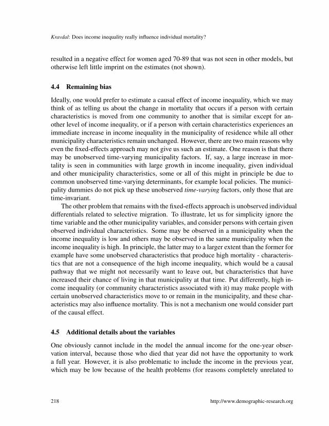
ipality dummies. This is seen in Table 1, where all effect estimates for women at age70-79 are shown as an example, and in Table 2, where only the effects of the Gini co-efficients are shown. There was a clear age pattern: The higher the age, the weaker theincome-inequality effect.

All these effects of income inequality in the simplest models were significant. We donot know how large the standard errors would have been if it had been possible to followthe common strategy and add a municipality-level random term, but it is worth noting thateven if they were twice as large as in the models with municipality dummies, the effectswould still be significant.

When the municipality dummies were added, the model fit improved significantly (thechanges in−2 log L were between 550 and 2300, which correspond to significance levelsbelow 0.01; values only shown in Table 1). On the whole, the income-inequality effectsbecame less positive, but there were some differences across age and sex (Table 2). Theeffects for men were only significantly adverse at age 30-39, and there were indicationalso at age 40-49, while the effects at higher ages were beneficial, or (for age 50-59) therewas at least an indication in that direction. Among women, there were no significanteffects at any age5.

Note that it would not be appropriate in this situation to just include a random term topick up unobserved municipality characteristics, which is typically done in multilevel epi-demiological research these days. That approach is based on a no-correlation assumptionthat is clearly violated.

Table 1: Effects (with standard errors) on the log-odds of all-cause mortalityamong women aged 70-79 in 1980-2002, according to discrete-timehazard models estimated from register data for the entire Norwe-gian population

Model without Model withmunicipality dummies municipality dummies

(’Fixed-effects model’)

Gini coefficient in the municipality 1.223 **** (0.079) 0.271 (0.178)Average income in the municipality (in 1000 NOK) 0.0015 **** (0.0001) 0.0007 (0.0006)Individual income (in 1000 NOK) −0.0038 **** (0.0001) −0.0038 **** (0.0001)

5 It might also be noted from Table 1 that the mortality-enhancing effect of high average income seen in thesimplest model disappeared in the fixed-effects model. This was found also for some other age groups, forboth sexes, but significant mortality-reducing effects, which are more in line with common expectations,were estimated for men aged 60-79 in the fixed-effects models (not shown).



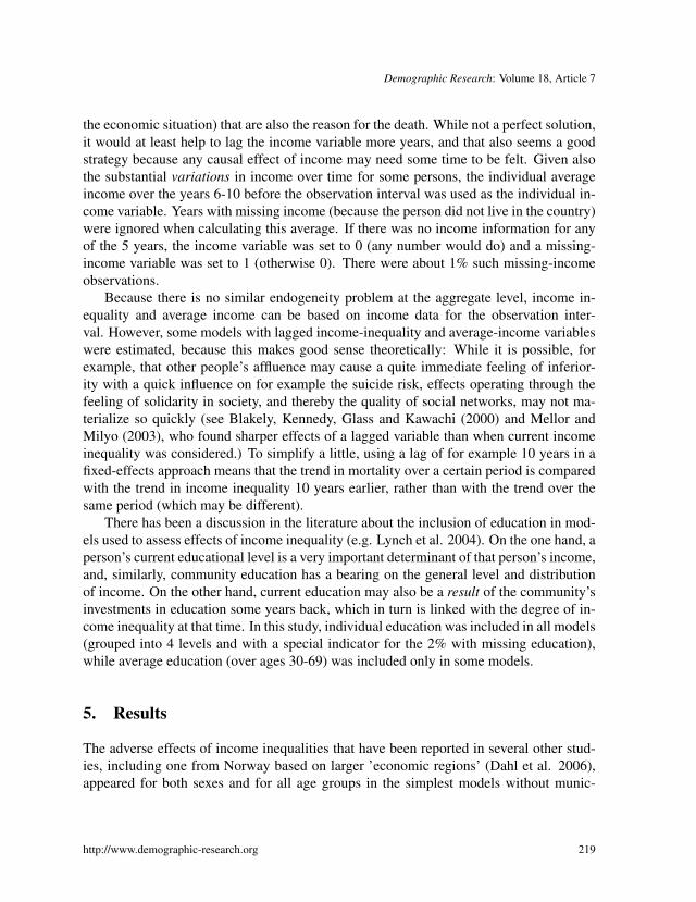
Table 1: (Continued)


(’Fixed-effects model’)Missing individual income

No a 0 0Yes 0.256 **** (0.073) 0.259 ** (0.073)

Education9 years a 0 010-12 years −0.184 **** (0.007) −0.179 **** (0.007)13-16 years −0.313 **** (0.016) −0.308 **** (0.016)17- years −0.182 *** (0.056) −0.178 *** (0.006)missing 0.075 *** (0.028) 0.075 *** (0.028)

Period1980 a 0 01981 −0.044 ** (0.020) −0.040 ** (0.020)1982 −0.081 **** (0.020) −0.069 **** (0.020)1983 −0.090 **** (0.020) −0.071 **** (0.020)1984 −0.130 **** (0.020) −0.105 **** (0.020)1985 −0.080 **** (0.020) −0.051 ** (0.020)1986 −0.154 **** (0.020) −0.118 **** (0.022)1987 −0.119 **** (0.020) −0.080 **** (0.022)1988 −0.136 **** (0.020) −0.089 **** (0.023)1989 −0.165 **** (0.020) −0.114 **** (0.023)1990 −0.135 **** (0.020) −0.075 *** (0.024)1991 −0.208 **** (0.020) −0.140 **** (0.025)1992 −0.232 **** (0.020) −0.158 **** (0.026)1993 −0.245 **** (0.020) −0.152 **** (0.029)1994 −0.292 **** (0.021) −0.204 **** (0.029)1995 −0.271 **** (0.021) −0.185 **** (0.030)1996 −0.327 **** (0.021) −0.241 **** (0.032)1997 −0.326 **** (0.021) −0.236 **** (0.035)1998 −0.353 **** (0.022) −0.261 **** (0.039)1999 −0.380 **** (0.022) −0.281 **** (0.042)2000 −0.408 **** (0.022) −0.304 **** (0.044)2001 −0.432 **** (0.023) −0.320 **** (0.046)2002 −0.410 **** (0.023) −0.301 **** (0.051)

Age (years) 0.105 **** (0.001) 0.105 **** (0.001)Municipality fixed effects Yes−2 Log L 1064731 1063424

a Reference category* p < 0.10; ** p < 0.05; *** p < 0.01; **** p < 0.001



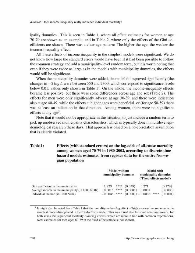
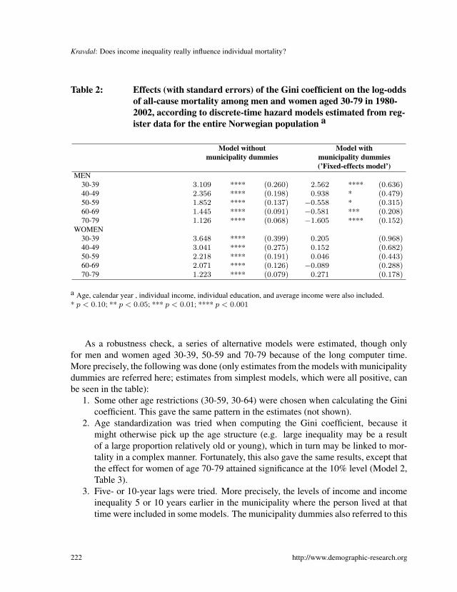
Table 2: Effects (with standard errors) of the Gini coefficient on the log-oddsof all-cause mortality among men and women aged 30-79 in 1980-2002, according to discrete-time hazard models estimated from reg-ister data for the entire Norwegian population a


(’Fixed-effects model’)MEN

30-39 3.109 **** (0.260) 2.562 **** (0.636)40-49 2.356 **** (0.198) 0.938 * (0.479)50-59 1.852 **** (0.137) −0.558 * (0.315)60-69 1.445 **** (0.091) −0.581 *** (0.208)70-79 1.126 **** (0.068) −1.605 **** (0.152)

WOMEN30-39 3.648 **** (0.399) 0.205 (0.968)40-49 3.041 **** (0.275) 0.152 (0.682)50-59 2.218 **** (0.191) 0.046 (0.443)60-69 2.071 **** (0.126) −0.089 (0.288)70-79 1.223 **** (0.079) 0.271 (0.178)

a Age, calendar year , individual income, individual education, and average income were also included.* p < 0.10; ** p < 0.05; *** p < 0.01; **** p < 0.001

As a robustness check, a series of alternative models were estimated, though onlyfor men and women aged 30-39, 50-59 and 70-79 because of the long computer time.More precisely, the following was done (only estimates from the models with municipalitydummies are referred here; estimates from simplest models, which were all positive, canbe seen in the table):

1. Some other age restrictions (30-59, 30-64) were chosen when calculating the Ginicoefficient. This gave the same pattern in the estimates (not shown).

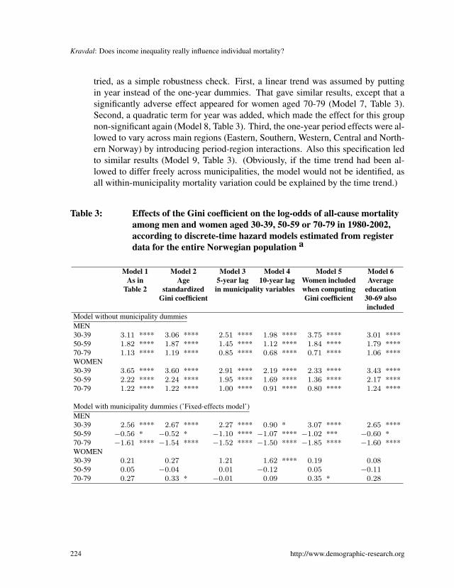
2. Age standardization was tried when computing the Gini coefficient, because itmight otherwise pick up the age structure (e.g. large inequality may be a resultof a large proportion relatively old or young), which in turn may be linked to mor-tality in a complex manner. Fortunately, this also gave the same results, except thatthe effect for women of age 70-79 attained significance at the 10% level (Model 2,Table 3).

3. Five- or 10-year lags were tried. More precisely, the levels of income and incomeinequality 5 or 10 years earlier in the municipality where the person lived at thattime were included in some models. The municipality dummies also referred to this



municipality. With a 5-year lag, the results were very similar, but the point estimatefor women aged 30-39 was more positive, and a more clearly significant beneficialeffect appeared for men aged 50-59 (Model 3, Table 3). With a 10-year lag, thisadverse effect for the youngest women turned significant, while the adverse effectfor the youngest men was now only significant at the 10% level (Model 4, Table 3).Also inclusion of average income and income inequality 5 or 10 years earlier in themunicipality where the person lived at the start of the observation interval (ratherthan 5 or 10 years earlier), gave very similar results (not shown). The data did notallow experimentation with lags longer than 10 years.

4. Women were included when calculating the Gini coefficient. Once again, the samepattern showed up in the mortality effect estimates, though there was a clearer indi-cation of an adverse effect among women aged 70-79 and the effect for men aged50-59 was more strongly significant (Model 5, Table 3).

5. Average education at age 30-69 was added to the model, which had no impact onthe estimated effects of the Gini coefficient (Model 6, Table 3). (According to themodel with municipality dummies, a high average education at age 30-69 reducedmortality significantly among women at age 50-59. Otherwise, this variable had noeffect.)

6. The average income among men was included, rather than that for both sexespooled. This gave the same pattern in the estimates (not shown).

7. Generally, inclusion of individual income makes the effects of inequality less pos-itive or more negative, but the differences are rather small (not shown). To seewhether a better control for individual income would be important, a grouped vari-able with 13 categories, including one for 0 income, was tried as an alternative. Thisgave very similar results (not shown). Shorter lags were also tried. For example, theinclusion of income 1-5 years before, rather than 6-10 years before, led to nearlythe same estimates (not shown). For men and women at age 70-79, an additionalmodel included average annual income during an earlier period, age 50-59, whenat least the men were very likely to have worked (excluding years before 1968, forwhich the income is not known, or any year abroad). Earlier labour incomes maythemselves be important, in addition to determining the level of the retirement pen-sions. A strongly significant beneficial effect of high income inequality was stillseen among men, while a harmful effect showed up for women, now significant atthe 5% level (not shown).

8. As explained earlier, the essence of the fixed-effects approach is that some of thewithin-municipality variation in mortality is attributed to an income-inequality ef-fect and some to a general change in mortality due to other factors. One mightsuspect that the results are influenced by the assumptions about this general mor-tality trend. Therefore, three alternative specifications of the period effect were



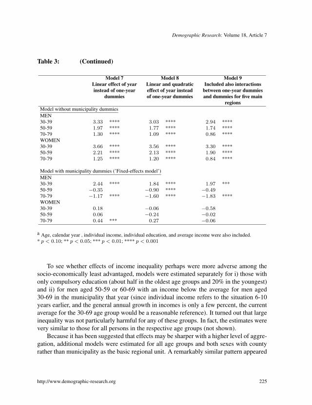
tried, as a simple robustness check. First, a linear trend was assumed by puttingin year instead of the one-year dummies. That gave similar results, except that asignificantly adverse effect appeared for women aged 70-79 (Model 7, Table 3).Second, a quadratic term for year was added, which made the effect for this groupnon-significant again (Model 8, Table 3). Third, the one-year period effects were al-lowed to vary across main regions (Eastern, Southern, Western, Central and North-ern Norway) by introducing period-region interactions. Also this specification ledto similar results (Model 9, Table 3). (Obviously, if the time trend had been al-lowed to differ freely across municipalities, the model would not be identified, asall within-municipality mortality variation could be explained by the time trend.)

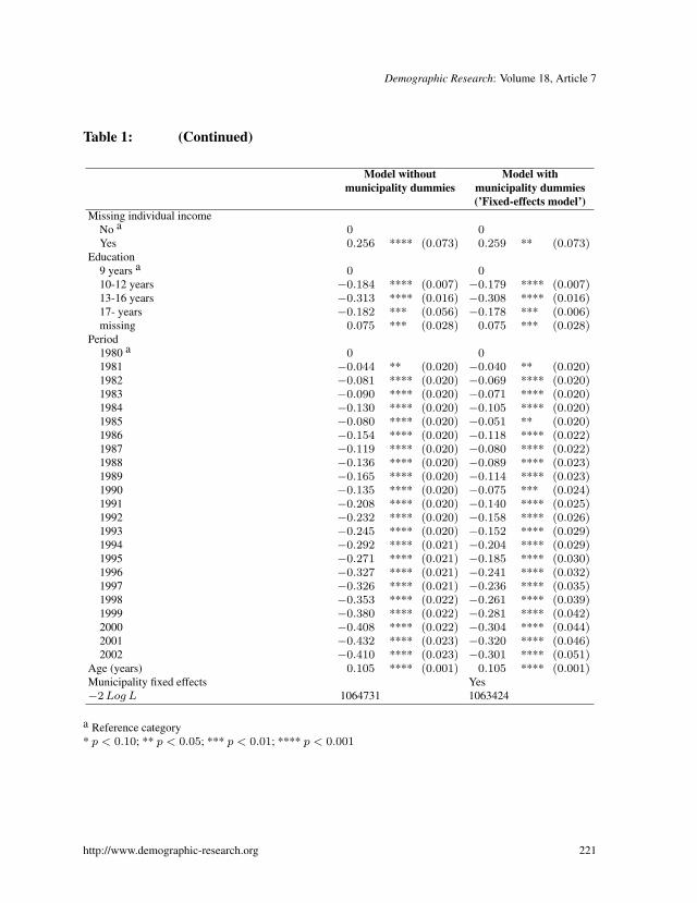
Table 3: Effects of the Gini coefficient on the log-odds of all-cause mortalityamong men and women aged 30-39, 50-59 or 70-79 in 1980-2002,according to discrete-time hazard models estimated from registerdata for the entire Norwegian population a

Model 1 Model 2 Model 3 Model 4 Model 5 Model 6As in Age 5-year lag 10-year lag Women included Average

Table 2 standardized in municipality variables when computing educationGini coefficient Gini coefficient 30-69 also

includedModel without municipality dummiesMEN30-39 3.11 **** 3.06 **** 2.51 **** 1.98 **** 3.75 **** 3.01 ****50-59 1.82 **** 1.87 **** 1.45 **** 1.12 **** 1.84 **** 1.79 ****70-79 1.13 **** 1.19 **** 0.85 **** 0.68 **** 0.71 **** 1.06 ****WOMEN30-39 3.65 **** 3.60 **** 2.91 **** 2.19 **** 2.33 **** 3.43 ****50-59 2.22 **** 2.24 **** 1.95 **** 1.69 **** 1.36 **** 2.17 ****70-79 1.22 **** 1.22 **** 1.00 **** 0.91 **** 0.80 **** 1.24 ****

Model with municipality dummies (’Fixed-effects model’)MEN30-39 2.56 **** 2.67 **** 2.27 **** 0.90 * 3.07 **** 2.65 ****50-59 −0.56 * −0.52 * −1.10 **** −1.07 **** −1.02 *** −0.60 *70-79 −1.61 **** −1.54 **** −1.52 **** −1.50 **** −1.85 **** −1.60 ****WOMEN30-39 0.21 0.27 1.21 1.62 **** 0.19 0.0850-59 0.05 −0.04 0.01 −0.12 0.05 −0.1170-79 0.27 0.33 * −0.01 0.09 0.35 * 0.28



Table 3: (Continued)

Model 7 Model 8 Model 9Linear effect of year Linear and quadratic Included also interactionsinstead of one-year effect of year instead between one-year dummies

dummies of one-year dummies and dummies for five mainregions

Model without municipality dummiesMEN30-39 3.33 **** 3.03 **** 2.94 ****50-59 1.97 **** 1.77 **** 1.74 ****70-79 1.30 **** 1.09 **** 0.86 ****WOMEN30-39 3.66 **** 3.56 **** 3.30 ****50-59 2.21 **** 2.13 **** 1.90 ****70-79 1.25 **** 1.20 **** 0.84 ****

Model with municipality dummies (’Fixed-effects model’)MEN30-39 2.44 **** 1.84 **** 1.97 ***50-59 −0.35 −0.90 **** −0.4970-79 −1.17 **** −1.60 **** −1.83 ****WOMEN30-39 0.18 −0.06 −0.5850-59 0.06 −0.24 −0.0270-79 0.44 *** 0.27 −0.06

a Age, calendar year , individual income, individual education, and average income were also included.* p < 0.10; ** p < 0.05; *** p < 0.01; **** p < 0.001

To see whether effects of income inequality perhaps were more adverse among thesocio-economically least advantaged, models were estimated separately for i) those withonly compulsory education (about half in the oldest age groups and 20% in the youngest)and ii) for men aged 50-59 or 60-69 with an income below the average for men aged30-69 in the municipality that year (since individual income refers to the situation 6-10years earlier, and the general annual growth in incomes is only a few percent, the currentaverage for the 30-69 age group would be a reasonable reference). It turned out that largeinequality was not particularly harmful for any of these groups. In fact, the estimates werevery similar to those for all persons in the respective age groups (not shown).

Because it has been suggested that effects may be sharper with a higher level of aggre-gation, additional models were estimated for all age groups and both sexes with countyrather than municipality as the basic regional unit. A remarkably similar pattern appeared



(not shown). The only difference worth mentioning is that, when the municipality dum-mies were included, the effect among women at age 70-79 was more markedly adverse(point estimate 0.77, significance level <0.01).

Finally, models were estimated for a few specific causes of death for which earlierstudies have suggested particularly adverse effects of income inequality, or of low so-cial cohesion (see also Martikainen et al. 2003): Alcohol related deaths, suicide, and allviolent deaths pooled. There were no harmful effects in any of these models when mu-nicipality dummies were included (not shown). Homicide was not considered separately,since there were only about 50 such deaths in the country each year.

6. Summary and Conclusion

Norway is a more egalitarian country than most others, and a low level of aggregation waschosen in this analysis. Nevertheless, significantly adverse effects of income inequality(net of the persons’ individual income) were estimated for all age groups and both sexes inthe model without municipality dummies. The effects were sharpest among the youngest.Perhaps inferiority is less intensely felt at the higher ages, or perhaps the psychosocialand other factors potentially influenced by income inequality have more effect on thecauses of death occurring relatively frequently at low ages, such as violent deaths. In thatcase, however, one would expect stronger effects on these causes of death in the modelsestimated for the older men and women, which did not appear.

It is interesting to see that the adverse effects of income inequality among the youngestsurvived the addition of municipality dummies (significant for women aged 30-39 whenthe income-inequality variable was lagged 10 years, and for men when there was no lag).Besides, there were indications in the same direction for men in their 40s, and adverseeffects appeared for 70-79 year old women with certain model specifications. Apart fromthat, this fixed-effects approach did not support the idea that high income inequality isharmful, and among older men (and among older women when the 5 largest municipalitieswere left out), there even seemed to be beneficial effects.

Non-positive effects are not theoretically implausible. As mentioned earlier, the com-mon ideas about causal mechanisms can be criticised. For example, can we be so sure thatincome inequality really undermines social cohesion substantially, or that it is responsiblefor generally stressful feelings of relative deprivation? Does weakened social cohesionreally exert the allegedly harmful health effect? Is it actually the case that rich people canblock poorer people’s interest in improving social services? In fact, one may even findarguments for beneficial effects. However, it is not easy to understand why the adverse aswell as the beneficial effects should be particularly pronounced for men.

Admittedly, there are some weaknesses in data and methods. One limitation is that



the municipality dummies only pick up the constant unobserved factors that may have abearing on both income inequality and individual mortality, such as for example environ-mental characteristics. The estimates may in principle be biased because of unobservedtime-varying community factors and selective migration. Further, the measurement ofincome is not ideal. It is the individual gross labour income that is available rather thanhousehold disposable income. Control for individual income appeared not to be very im-portant, so the key issue is probably whether a Gini coefficient computed from individualincomes is a sufficiently relevant indicator of inequality. Fortunately, the fact that it didnot matter whether women’s incomes were included when computing the Gini coefficientsuggests a certain robustness. It should also be noted that only the importance of cur-rent inequality or that 5 or 10 years earlier has been assessed. In lack of data, effectsof inequality in earlier years could not be analysed. Finally, there is always a possibilitythat other specifications of the control variables, and perhaps especially the period effect,might have led to markedly different results, though the few alternatives that were triedsupported the main conclusion.

With due respect to these potential problems, there are two main contributions fromthis study. First, it has added to the doubts about the existence of a generally adverseeffect of income inequality, at least in the Nordic setting. Second, it has illustrated thatone perhaps should be more careful when interpreting the results from the cross-sectionalmodels (with or without a random term) that traditionally are employed in such inves-tigations, and that it may be worthwhile in the future - unless several relevant controlvariables can be included - to construct longitudinal data that allow researchers to useregional dummies to control for unobserved factors at the same level of aggregation asthe income inequality is measured.

7. Acknowledgements

The financial support from the Norwegian Research Council and the comments fromMark Montgomery, two anonymous reviewers and an associate editor, Jutta Gampe, aregreatly appreciated.



References

Backlund, E., Rowe, G., Lynch, J., Wolfson, M., Kaplan, G., and Sorlie, P. (2007). Incomeinequality and mortality: A multilevel prospective study of 521248 individuals in 50states. International Journal of Epidemiology, 36:590–596.

Beckfield, J. (2004). Does income inequality harm health? New cross-national evidence.Journal of Health and Social Behavior, 45:231–248.

Blakely, T., Kennedy, B., Glass, R., and Kawachi, I. (2000). What is the lag time betweenincome inequality and health status? Journal of Epidemiology and Community Health,54:318–319.

Blomgren, J., Martikainen, P., Mäkelä, P., and Valkonen, T. (2004). The effects of regionalcharacteristics on alcohol-related mortality - a register-based multilevel analysis of 1.1million men. Social Science and Medicine, 58:2523–2535.

Dahl, E., Elstad, J., Hofoss, D., and Martin-Mollard, M. (2006). For whom is incomeinequality most harmful? A multi-level analysis of income inequality and mortality inNorway. Social Science and Medicine, 63:2562–2574.

Ellaway, A. and Macintyre, S. (2001). Women in their place. gender and perceptionsof neighbourhoods and health in the west of Scotland. In Dyck, I., Lewis, D., andMcLafferty, S., editors, Geographies of Women’s Health., pages 265–281. London:Routledge.

Franzini, L., Ribble, J., and Spears, W. (2001). The effects of income inequality andincome level on mortality vary by population size in Texas countries. Journal of Healthand Social Behavior, 42:373–387.

Gerdtham, U.-G. and Johannesson, M. (2004). Absolute income, relative income, incomeinequality, and mortality. Journal of Human Resources, 39:228–247.

Gertler, P. and Molyneaux, J. (1994). How economic development and family planningprograms combined to reduce Indonesian fertility. Demography, 31:33–63.

Goldstein, H. (2003). Multilevel Statistical Models, 3 edition. London: Arnold.Helleringer, S. and Kohler, H. (2005). Social networks, perceptions of risk, and chang-

ing attitudes towards HIV/AIDS: New evidence from a longitudinal study using fixedeffects analysis. Population Studies, 59:265–282.

Islam, M., Merlo, J., Kawachi, I., Lindström, M., Burström, K., and Gerdtham, U. (2006).Does it really matter where you live? A panel data multilevel analysis of Swedishmunicipality-level social capital on individual health-related quality of life. HealthEconomics, Policy and Law, 1:209–235.

Kautto, M., Heikkilä, M., Hvinden, B., and Marklund, S., editors (1999). Nordic SocialPolicy. Changing Welfare States. London: Routledge.

Kavanagh, M., Bentley, R., Turrell, G., Bromm, D., and Subramanian, S. (2006). Doesgender modify associations between self rated health and the social and economic char-



acteristics of local environments? Journal of Epidemiology and Community Health,60:490–495.

Kawachi, I. (2000). Income inequality and health. In Berkman, L. and Kawachi, I.,editors, Social Epidemiology, pages 76–93. New York: Oxford University Press.

Kawachi, I. and Berkman, L. (2000). Social cohesion, social capital and health. InBerkman, L. and Kawachi, I., editors, Social Epidemiology, pages 174–190. New York:Oxford University Press.

Kravdal, Ø.. (1995). Is the relationship between childbearing and cancer incidence due tobiology or lifestyle? Examples of the importance of using data on men. InternationalJournal of Epidemiology, 24:477–484.

Kravdal, Ø. (2000). Social inequalities in cancer survival. Population Studies, 54:1–18.Kravdal, Ø. (2007). A fixed-effects multilevel analysis of how community family struc-

ture affects individual mortality in Norway. Demography, 44:519–536.Lobmayer, P. and Wilkinson, R. (2002). Inequality, residential segregation by income, and

mortality in US cities. Journal of Epidemiology and Community Health, 56:183–187.Lynch, J., Smith, G. D., Harper, S., Hillemeier, M., Ross, N., Kaplan, G., and Wolfson, M.

(2004). Is income inequality a determinant of population health? Part 1. A systematicreview. The Milbank Quarterly, 82:5–99.

Martikainen, P., Kauppinen, T., and Valkonen, T. (2003). Effects of the characteristics ofneighbourhoods and the characteristics of people on cause specific mortality: A regis-ter based follow-up study of 252000 men. Journal of Epidemiology and CommunityHealth, 57:210–217.

Martikainen, P., Maki, N., and Blomgren, J. (2004). The effects of area and individualsocial characteristics on suicide risk: A multilevel study of relative contribution andeffect modification. European Journal of Population, 20:323–350.

Mellor, J. and Milyo, J. (2001). Reexamining the evidence of an ecological associationbetween income inequality and health. Journal of Health Politics, Policy and Law,26:487–522.

Mellor, J. and Milyo, J. (2002). Income inequality and health status in the United States.Evidence from Current Population Survey. Journal of Human Resources, 37:510–539.

Mellor, J. and Milyo, J. (2003). Is exposure to income inequality a public health con-cern? Lagged effects of income inequality on individual and population health. HealthServices Research, 38:137–152.

Mohan, J., Twigg, L., Barnard, S., and Jones, K. (2005). Social capital, geography andhealth: A small-area analysis for England. Social Science and Medicine, 60:1267–1283.

Molinari, C., Ahern, M., and Hendryx, M. (1998). The relationship of community qualityto the health of women and men. Social Science and Medicine, 47:1113–1120.

Montgomery, M. and Casterline, J. (1996). Social learning, social influence and new



models of fertility. Population and Development Review, 22(suppl):151–175.Nielsen, F. and Alderson, A. (1997). The Kuznets curve and the great U-turn: Income

inequality in the US counties, 1970 to 1990. American Sociological Review, 62:12–33.Osler, M., Christensen, U., Due, P., Lund, R., Andersen, I., Diderichsen, F., and Prescott,

E. (2003). Income inequality and ischaemic heart disease in Danish men and women.International Journal of Epidemiology, 32:375–380.

Osler, M., Prescott, E., Gronbak, M., Christensen, U., Due, P., and Engholm, G. (2002).Income inequality, individual income, and mortality in Danish adults: Analysis ofpooled data from two cohort studies. British Medical Journal, 324:13–16.

Portes, A. (1998). Social capital: Its origins and applications in modern sociology. AnnualReview of Sociology, 24:1–24.

Rindfuss, R., Guilkey, D., Morgan, S., Kravdal, Ø., and Guzzo, K. (2007). Child careavailability and first-birth timing in Norway. Demography, 44:345–372.

Rosenzweig, M. and Wolpin, K. (1986). Evaluating the effects of optimally distributedpublic programs: Child health and family planning interventions. American EconomicReview, 76:470–482.

Scheffler, R., Brown, T., and Rice, J. (2007). The role of social capital in reducing non-specific psychological distress: The importance of controlling for omitted variable bias.Social Science and Medicine, 65:842–854.

Stafford, M., Cummins, S., Macintyre, S., Ellaway, A., and Marmot, M. (2005). Genderdifferences in the association between health and neighbourhood environment. SocialScience and Medicine, 60:1681–1692.

Statistics Norway (2007). Online at http://www.ssb.no/emner/02/02/10/dode/tab-2007-04-26-06.html.

Sundquist, J., Johansson, S., Yang, M., and Sundquist, K. (2006). Low linking socialcapital as a predictor of coronary heart disease in Sweden: A cohort study of 2.8 millionpeople. Social Science and Medicine, 62:954–963.

United Nations (2006). Inequality in income or consumption. In Human DevelopmentReports. Online at http://hdr.undp.org/statistics/data/indicators.cfm?x=148&y=2&z=1.

Veenstra, G. (2005). Location, location, location: Contextual and compositional healtheffects of social capital in British Columbia, Canada. Social Science and Medicine,60:2059–2071.

Wagstaff, A. and van Doorslaer, E. (2000). Income inequality and health: What does theliterature tell us? Annual Review of Public Health, 21:543–567.

Wen, M., Browning, C., and Cagney, K. (2003). Poverty, affluence, and income inequal-ity: Neighborhood economic structure and its implications for health. Social Scienceand Medicine, 57:843–860.

Wilkinson, R. and Pickett, K. (2006). Income inequality and population health: A reviewand explanation of the evidence. Social Science and Medicine, 62:1768–1784.



Appendix

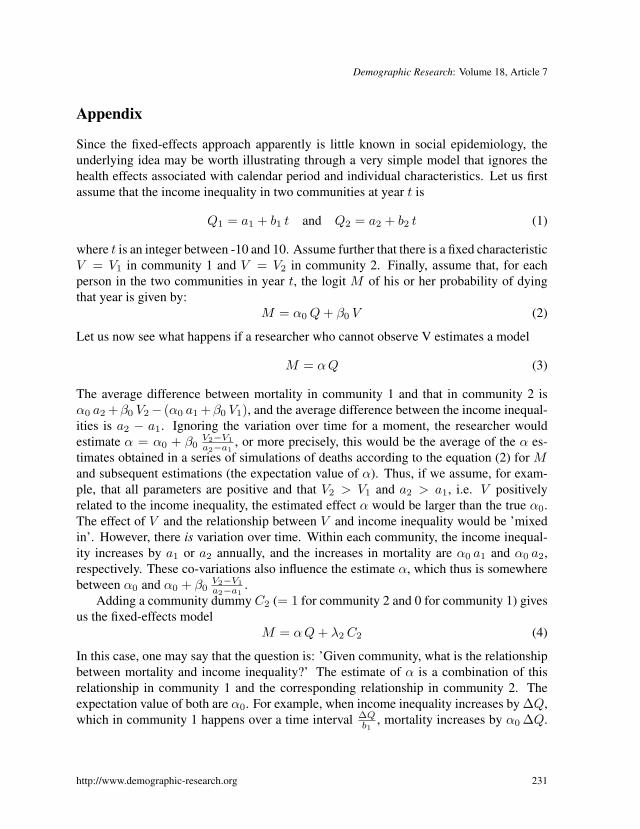
Since the fixed-effects approach apparently is little known in social epidemiology, theunderlying idea may be worth illustrating through a very simple model that ignores thehealth effects associated with calendar period and individual characteristics. Let us firstassume that the income inequality in two communities at year t is

Q1 = a1 + b1 t and Q2 = a2 + b2 t (1)

where t is an integer between -10 and 10. Assume further that there is a fixed characteristicV = V1 in community 1 and V = V2 in community 2. Finally, assume that, for eachperson in the two communities in year t, the logit M of his or her probability of dyingthat year is given by:

M = α0 Q + β0 V (2)

Let us now see what happens if a researcher who cannot observe V estimates a model

M = α Q (3)

The average difference between mortality in community 1 and that in community 2 isα0 a2 +β0 V2− (α0 a1 +β0 V1), and the average difference between the income inequal-ities is a2 − a1. Ignoring the variation over time for a moment, the researcher wouldestimate α = α0 + β0

V2−V1a2−a1

, or more precisely, this would be the average of the α es-timates obtained in a series of simulations of deaths according to the equation (2) for Mand subsequent estimations (the expectation value of α). Thus, if we assume, for exam-ple, that all parameters are positive and that V2 > V1 and a2 > a1, i.e. V positivelyrelated to the income inequality, the estimated effect α would be larger than the true α0.The effect of V and the relationship between V and income inequality would be ’mixedin’. However, there is variation over time. Within each community, the income inequal-ity increases by a1 or a2 annually, and the increases in mortality are α0 a1 and α0 a2,respectively. These co-variations also influence the estimate α, which thus is somewherebetween α0 and α0 + β0

V2−V1a2−a1

.Adding a community dummy C2 (= 1 for community 2 and 0 for community 1) gives

us the fixed-effects modelM = α Q + λ2 C2 (4)

In this case, one may say that the question is: ’Given community, what is the relationshipbetween mortality and income inequality?’ The estimate of α is a combination of thisrelationship in community 1 and the corresponding relationship in community 2. Theexpectation value of both are α0. For example, when income inequality increases by ∆Q,which in community 1 happens over a time interval ∆Q

b1, mortality increases by α0 ∆Q.



γ2 picks up the average difference between the communities that is not due to incomeinequality and is β0 (V2 − V1).

To summarize and generalize, the effect of income inequality on mortality is identi-fied exclusively from the within-community correlations between income inequality andmortality when community dummies are included. The between-community differencesin mortality, which may be influenced by stable unobserved factors also affecting incomeinequality, do not contribute at all to the identification of the income-inequality effect.Note, however, that - regardless of whether there actually are such stable unobserved con-founders - one does not ’take away’ any of income-inequality effect by doing this. It is thetrue effect (α0) that appears, just as if the unobserved factor (V ) could be included ratherthan the community dummy (in which case information about both within-communityand between-community differences had been used).


Does income inequality really influence individual mortality? Results

Documents

Transcript of Does income inequality really influence individual mortality? Results