Does Firm Investment Respond to Peers’ Investment?2017-5-24 · Electronic copy available at :...

Electronic copy available at: https://ssrn.com/abstract=2827803

Does Firm Investment Respond to Peers’ Investment?

M. Cecilia Bustamante and Laurent Fresard∗

January 22, 2017

ABSTRACT

Yes, it responds positively. Using a new instrumental variable based on the pres-ence of location-specific information externalities, we estimate that firms increase in-vestment by 10% in response to a one standard-deviation increase in the investment oftheir product market peers. The influence of peers’ investment is stronger in concen-trated industries, featuring more heterogeneous firms, and for relatively smaller firmsthat possess less precise information. These findings are consistent with a model inwhich firms compete and use peers’ investment as a source of information about prod-uct market fundamentals. The positive influence of peers’ investment could amplifyvariation in aggregate investment and thus affect productivity and output.

∗University of Maryland. Corresponding author: Laurent Fresard, Robert H. Smith School of Business,University of Maryland, 4425 Van Munching Hall, College Park, MD 20742, Tel: 301 405 9639, email:[email protected]. For helpful comments, we thank Jean-Noel Barrot, Jonathan Berk, DonaldBowen, Will Cong, Julien Cujean, Francesco D’Acunto, Olivier Dessaint, Murray Frank, Xavier Giroud, MaxMaksimovic, Rich Mathews, Adrien Matray, Venky Venkateswaran, Chris Parsons, Nagpurnanand Prabhala,Shri Santosh, Giorgo Sertsios, Kelly Shue, Philip Valta and seminar participants at the MIT Junior FinanceConference, the UBC Summer Finance Conference, the University of Minnesota, and the UTDT SummerConference for useful comments and suggestions. We thank Jerry Hoberg and Gordon Phillips for sharingtheir TNIC data. A previous version of the paper circulated under the title ”What Explains the ProductMarket Component of Corporate Investment”. All errors are our own.


I Introduction

Corporate investment is positively correlated within industries.1 This empirical fact might

simply indicate that firms selling similar products or services are exposed to the same funda-

mental shocks, which lead them to passively invest alike. The commonality of firms’ invest-

ment could also result from “peer effects”, whereby firms’ investment is actively influenced

by that of their product market peers. Deciphering the origins of investment commonality

is important since, unlike exposure to common shocks, the presence of peer effects could

amplify (or attenuate) the effect of firm-specific shocks within and across industries, and

therefore affects the dynamics of aggregate investment.

Attributing the interdependence of firms’ investments to peer effects is difficult for both

theoretical and empirical reasons. First, peer effects can originate from different economic

channels, leading some firms to respond positively to peers’ investment, and others to respond

negatively. In learning models for instance, imperfectly informed firms respond positively

to peers’ investment because firms use peers’ decisions as a source of information about

investment opportunities (Bikhchandani, Hirshleifer, and Welch (1992)). In contrast, in in-

vestment models featuring strategic interactions, firms’ respond negatively to the investment

of peers when peers’ competitive actions hurt their prospects (Fudenberg and Tirole (1984)).

Second, identifying peers effects in the data requires isolating firms’ responses to the deci-

sions of their peers from correlated decisions due to common information among related firms

(Manski (1993) or Glaeser, Sacerdote, and Scheinkman (2003)).

This paper provides direct evidence that firms’ investment respond positively to the

investment of their product market peers. To guide our tests, we develop a strategic model

of investment in which firms compete in the product market but have imperfect information

about fundamentals (e.g., future demand). The model serves three purposes. First, it

explains when and why peer effects arise in industry equilibrium. Second, it characterizes

the conditions for their empirical identification when firms’ information is imperfect. Third,

1For instance, based on our working sample of firms in Compustat between 1996 and 2011, the correlationbetween public firms’ investment and that of their product market peers ranges between 0.35 and 0.40depending on the definition of the industry group. Industry fixed effects explain more than 10% of the totalvariability in corporate investment.

1


it delivers novel testable predictions.

Our model builds on Gal-Or (1987) and features two firms A and B that offer differenti-

ated products and face an uncertain demand for their products. Firms invest in production

capacity, and future cash flows are determined by the chosen capacity (i.e. their investment)

and the resulting equilibrium price that firms can charge for their respective products. Be-

fore investing, each firm receives imperfect private information about future demand (i.e.,

the fundamental) that is positively correlated with the private information of the other firm.

Firms decide sequentially on how much to invest. Firm B receives its private information

and chooses its investment, strategically taking into account the equilibrium effect of the

future investment by firm A. Then, firm A chooses its investment after obtaining its private

information and observing the investment of firm B. In industry equilibrium, the investment

of firm A is a linear function of its private information and the investment of firm B. The

theoretical influence of B’s investment – the “equilibrium” peer effect – can be either posi-

tive or negative, depending on the relative importance of the effects of learning from peers’

investments versus the strategic effect of peers’ investments.

We then use the model to show that an econometrician cannot identify the equilibrium

peer effect by regressing the investment of firm A on that of firm B, unless she perfectly

observes firms’ private information. Since the private information received by firm A is

correlated with the investment of firm B (firms’ private information is positively correlated),

we prove that an estimation by ordinary least squares introduces an upward bias, and the

magnitude of such bias depends on the precision of the econometrician’s knowledge about

firms’ private information. We conclude that the econometrician can correctly estimate the

equilibrium peer effect if she uses an instrument for the investment of firm B that (i) contains

information relevant for firm A’s investment, but (ii) is orthogonal to the private information

of firm A. Instrumentation in our setting has to isolate variation in information relevant

for firm A’s investment that is only possessed by firm B, and not variation in firm B’s

fundamentals that is orthogonal to that of firm A.2

In the spirit of Bartik (1991), we combine industry and geography variations to construct

2This is because firm A should not respond that the variation in firm B’s investment that is irrelevantfor its prospects. In this case, we do not expect to observe any peer effects.

2

an instrument satisfying these conditions. To illustrate, imagine that firms A and B man-

ufacture furniture and are located in Austin and Boston respectively. We use the average

investment of firms in Boston that operate in product markets that are unrelated to furni-

ture (e.g., optical equipment or footwear) as an instrument for the investment of firm B.

In the data, the average investment of unrelated firms located in Boston correlates strongly

with firm B’s investment, reflecting local knowledge diffusion, technology transfer, or con-

sumption externalities between neighboring firms operating in different industries (Glaeser,

Kallal, Scheinkman, and Shleifer (1992)).3 We argue that the local information leading to

investment commonality in Boston (e.g., shared information about business trends) is not

observed by firm A in Austin, but it is plausibly related to its future growth opportunities.

We estimate firms’ response to the investment of their peers on a large sample of more

than 6,000 public firms over the period 1996 to 2011. We define firms’ product market

peers using the Hoberg and Phillips (2015) industry definitions, and firms’ local peers as

firms headquartered in the same Metropolitan Statistical Area (MSA). To ensure that our

instrument truly removes the influence of common fundamentals, we construct it using only

unrelated non-local firms in order to purge direct and indirect horizontal and vertical links

among firms.

Using the average investment of non-local unrelated peers as an instrument for the average

investment of a firm’s non-local product market peers, we find that firms respond positively to

the investment of their product market peers. The economic magnitude of peers’ influence on

corporate investment is substantial. The average firm in the sample increases its investment

by 10% (compared to its average) in response to a one standard deviation increase in the

(instrumented) average investment of its product market peers.

Our identification could arguably be threatened if firms can directly observe the localized

information leading to investment commonality in other locations, or if the construction of

our instrument fails to completely purge economic links between firms and the unrelated

neighbors of their product market peers. To mitigate this concern, we artificially replace

3The idea that important knowledge and technology transfers occur between unrelated industries inspecific locations starts with Jacobs (1969), who argues that the variety and diversity of geographicallyproximate industries promote innovation and growth. Consistent with this idea, Ellison, Glaser, and Kerr(2010) show that industries co-agglomeration is related to the sharing of ideas and knowledge.

3

each true non-local product market peer in our sample (i.e., firm B) by a random firm that is

located in the same location as the true peer but operating in unrelated product markets (e.g.

a footwear manufacturer also located in Boston). Across 1,000 distinct artificial samples, we

find no evidence that firms’ investment (e.g., firm A in Austin) responds to the instrumented

investment of unrelated non-local firms (such as footwear manufacturer in Boston). The

insignificance of peer effects in these placebo samples are obtained despite strong first-stage

estimates, and therefore provide direct support for the validity of our instrumental variables

approach.

To further understand the nature of peer effects, we use the model to predict how the

equilibrium peer effect varies with the model’s parameters. We derive four unique predictions

and find empirical support for each of them using firm and industry-level proxies. First, the

model predicts that the equilibrium peer effect decreases with the relative precision of firm

A’s private information. In equilibrium, firm A relies more on the investment of firm B

as a source of information when its own information is relatively less precise. Second, the

equilibrium peer effect also decreases as firms’ private information becomes more correlated.

In that case, firm A puts less weight on the investment of firm B since a larger portion of

the information revealed through this investment is already known to firm A. Third, the

model further predicts that the equilibrium peer effect decreases with the relative size of

firm A (i.e., its initial capacity). Intuitively, a smaller firm has stronger incentives to learn

from its peer (increasing the equilibrium peer effect). Fourth, peers’ influence is predicted

to be larger in concentrated product markets, in which a fringe of smaller firms has stronger

incentives to learn from larger product market peers. These results confirm the importance

for firms to use peers’ investment as a source of strategic information.

Finally, we invalidate two possible alternative explanations for our findings. First, we

show that the influence of peers’ investment is unlikely to reflect herding behavior arising

because some managers are more favorably evaluated when they follow the decisions of their

peers than if they behave independently (Scharfstein and Stein (1990)). Second, we show

that our results cannot be explained by a scenario in which firms have perfect information

about their prospects and actions are strategic complements, as we find significant positive

4

peer influence in markets featuring competition in strategic substitutes (as in our model).

Our main contribution is to empirically establish that the investment of product market

peers has a direct positive influence on firms’ investment decisions, and to provide theory-

based evidence for why these peer effects arise in equilibrium. Our analysis thus adds to

existing research that shows that firms’ investment is positively associated with that of

geographically-close firms (Dougal, Parsons, and Titman (2015) and firms whose executives

share social ties (Shue (2013) and Fracassi (2016)). Other studies indicate that investment

is positively correlated within industries because firms over-react to common investment op-

portunities, either because they neglect the impact of competition on future profits (Hoberg

and Phillips (2010) and Greenwood and Hanson (2015)) or because they blend with the

crowd (Povel, Sertsios, Kosava, and Kumar (2015)). To the best of our knowledge, our pa-

per is the first to show that firms’s investment positively respond to that of their product

market peers, and to provide evidence that such peer effects arise because firms use peers’

investment to infer information about their prospects.

Our paper belongs to a growing literature examining peer effects in corporate decisions.4

We differ from most existing research by combining learning and strategic effects in a model of

investment to clarify possible economic mechanisms leading to peer effects within industries,

and to facilitate their empirical detection. Our theoretical and empirical analyses contribute

to the existing literature in showing that identification in settings where firms have imperfect

information and can learn from each other relies on exogenous variation in the information

they possess about their fundamentals, and not on exogenous variation in their fundamentals.

This distinction is important to correctly interpret empirical estimates.

4For instance, Lerner and Malmendier (2013) find peer effects in entrepreneurship; Leary and Roberts(2014) find evidence of peer effects in capital structure; Kaustia and Rantala (2015) report peer effects infirms’ decision to split their stocks; Bouwman (2011) finds that firms with shares directors have more similargovernance; Popadak (2012) finds that industry peers’ influence firms’ dividend policy; and Matray (2015)reports that innovation by one firm fosters innovation by neighboring firms.

5

II Equilibrium Peer Effects

A The Model

We adapt the model of Gal-Or (1987) to study a setting in which two firms A and B

offer differentiated products and have the ability to increase their production by investing

in additional physical capital. The model features two key ingredients. First, similar to

standard games of strategic interaction, the investment decision of one firm is strategic and

negatively affects the prospects of the other firm as an increased supply of products lowers the

equilibrium market prices. Second, both firms are imperfectly informed about future demand

for their products, but each firm can potentially learn information about the demand for its

own product by observing the investment decision of the other firm.

Firms’ cash flows. Both firms optimally decide on investment (i.e., choose their pro-

ductive capacity) by considering its impact on expected future cash flows in equilibrium. At

any point in time, the operating profits (π) of each firm i = A,B are given by:

πi [Ki, K−i, ε] ≡ pi [Ki, K−i, ε]×Ki (1)

where Ki is the installed capital of firm i, pi is the price that firm i charges for its product, and

ε is a common demand shock that affects the profits and investment decisions of both firms

in the market. For simplicity, we assume that firms’ production is equal to their installed

capital K, and that firms face no marginal costs of production. The unit price charged by

firm i is given by the following linear inverse demand function:

pi [Ki, K−i, ε] = α− γ ×Ki − θ ×K−i + ε, α, γ, θ > 0 (2)

where the parameter γ > 0 reflects the negative effect of the supply of firm i’s product on

its own price. The parameter θ > 0 indicates that firms’ products are strategic substitutes:

an increase in capacity by the rival firm affects the price of firm i negatively.5 The inverse

demand function in Equation (2) further allows for product differentiation, such that each

firm can charge a slightly different price for its own product. To capture this feature, we

follow Singh and Vives (1984) and assume that the influence of a firm’s production (Ki) on

5We analyze the alternative case in which θ < 0 and goods are strategic complements in Section V.

6

its product price (pi) is weakly stronger than the influence of its rivals’ production (K−i),

such that γ ≥ θ. The price charged by both firms is the same and their products are perfect

substitutes in the special case in which γ = θ.

We define investment as the ratio of investment to capital Ii ≡ K+i /K

−i −1, which reflects

the change in the installed capital of firm i from an initial stage in which firms operate with

capital K−i > 0, to a subsequent stage in which firms operate with capital K+i . We take the

initial installed capacity K−i as given, and use the superscripts − and + to denote before and

after investment, respectively. When firms modify their capital stock, they are subject to

the following cost:

Φ[Ii, K

−i

]= κ× Ii ×K−i +

φ

2× (Ii)

2 ×K−i (3)

where κ > 0 is the price of purchasing capital. Following Abel and Eberly (1994), the second

term in Equation (3) captures convex costs of investment such that φ > 0.

Sequence of actions. We assume that firms have imperfect information about the

future demand shock ε in Equation (2), as a mean of arguing in reduced form that firms are

imperfectly informed about the value of their growth opportunities. When firms decide on

investment, the future demand shock ε is unknown, but they receive a private signal si that

contains imperfect information about ε. As a result, firms’ investment decisions may reveal

information about the private information they possess. To study the propensity for a firm

to condition its own investment on that of its peer, we assume that firms invest sequentially.

The sequence of decisions in the model contains three stages as shown in Figure 1. First,

firm B receives its private signal sB, and chooses its investment IB. Second, firm A receives

its private signal sA, observes IB, and then chooses its investment IA. Once firms have

committed to their corresponding strategies, investments are undertaken, the demand shock

materializes, and cash flows are realized.

[Insert Figure 1 about Here]

Information structure. We assume that firms’ private signal si does not contain

information about the product market’s demand as a whole, but rather about a portion of

the demand. For instance, firms may possess proprietary information concerning the future

7

demand pertaining to their geographical area, or for a given segment of customers (e.g.,

young or female customers). We denote by εi the demand shock related to the portion of

the market observed by firm i, and we assume that the private signal si is a signal about

the demand shock εi. The overall market demand shock ε in Equation (2) is then equal to

ε ≡ (εA + εB) /2. In other words, the demand shock ε that influences equilibrium prices in

the product market is given by the average portion-specific shock about which firms receive

private signals.6

Consistent with standard models of imperfect information (Welch (1992)), firms are im-

perfectly informed about the demand shock ε, but they know its underlying distribution.

We assume that E[εi] = µ > 0 such that the shocks to the alternative portions of the market

have identical means, as well as V ar [εi] = 1 > 0. In addition, the demand shocks affecting

the portions of the market observed by each firm are such that cov [εA, εB] ≡ ρ > 0. The pa-

rameter ρ thus captures both the covariance and the correlation between the portion-specific

demand shocks εA and εB.7 We require ρ 6= 0 to ensure that a fully revealing equilibrium

exists and we focus on the case ρ > 0 to simplify exposition.

Firms also know the underlying distribution of the signals they receive. We assume that

the private signal received by each firm si is an unbiased but noisy estimator of the demand

shock εi. As a result, the expected value and the variance of si are such that E [si| εi] = εi

and V ar [si| εi] = σ2i < ∞, respectively. The corresponding signal precision is given by

1/σ2i > 0. Furthermore, the correlation between the portion-specific shocks εi implies that

firms’ private signals are correlated. When 0 < ρ < 1, firms’ private signals si are partially

correlated. When ρ = 1, the shocks εi are perfectly correlated such that each private signal

si is the sum of the common demand shock ε and additional white noise.

Last, we need not impose a specific prior distribution function of the shocks εi, nor

a specific posterior distribution function of the signals si. We assume instead that these

6We define ε using a simple average of εA and εB for analytical convenience. It can be shown thatany weighted average of the shocks εi (i.e. weighted by the relative product differentiation) yields the sameresults shown in this paper. This is because the demand function is linear in the demand shock ε.

7The parameter ρ captures within-industry co-movement in demand shocks. Note however that sincethe portions of the market observed by firms A and B may overlap, the parameter ρ may simply capturesuch overlap.

8

distribution functions yield linear posterior expectations on the future demand. Moreover, we

require that the posterior distributions of the signals si for each firm have the same functional

form. Several sets of prior and posterior distributions comply with these properties.8

Other assumptions. We make additional parametric assumptions that are without

loss of generality and help us simplify exposition. We set α = κ to reduce the number of

parameters in the model. We assume firms discount cash flows at a rate equal to zero and

invest positive amounts. We thus impose a lower bound on the expected demand shock such

that µ > µ.9 Intuitively, the expected demand shock should not be too low for investment

to stay positive. Last, we require σ2B < 2ρ− 1; the reason why this constraint is analytically

convenient is clarified in the Appendix.

B Investment in Industry Equilibrium

We solve for firms’ equilibrium investment decisions, assuming that each firm chooses the

level of investment that maximizes its value. The equilibrium concept is Nash-Cournot, and

we provide all proofs in the Appendix.

To better understand the derivation of the equilibrium, consider first the investment

decision of firm A. Firm A chooses IA given its private signal sA and the observed investment

of firm B (IB). As a result, the problem of firm A is given by:

maxIA≡K+

A/K−A−1

E[π+A

[K+A , K

+B , ε]− ΦA

[IA, K

−A

]∣∣ sA, IB] , (4)

where we set π−i for i = A,B equal to zero without loss of generality. The solution to

Equation (4) yields the reaction function of firm A, which we define as IRA [IB, sA]. Firm

B chooses its investment before firm A, taking into account both its private signal and the

reaction function of its peer:

maxIB≡K+

B/K−B−1

E[π+B

[K+B , K

+A , ε]− ΦB

[IB, K

−B

]∣∣ sB, IRA ] . (5)

8For instance, these properties hold when both εi and si| εi are normally distributed. Since εi are definedas demand shocks to (strictly positive) prices, an alternative specification that yields linear conditionalexpectations with non-negative values is a Gamma distribution for εi and a Poisson distribution for si| εi.

9The expression for µ is provided in Equation (17) in the Appendix. The inequality µ > µ is a necessarycondition such that the investment to capital ratio IB is positive in equilibrium. We impose IB > 0 to betterinterpret the reaction of firm A to firm B’s investment decision in equilibrium. Investment in our workingsample is also pervasively positive.

9

Consistent with standard games of strategic interaction, Equation (5) indicates that firm B

chooses investment by taking into account the optimal reaction of firm A to its investment

IB. Unlike standard games of strategic interaction, however, the reaction function IRA is itself

a function of the private signal received by firm B, through IB.

Proposition 1. [Equilibrium Investment Strategies] The unique pure strategy equilibrium issuch that:

IB [sB] = δB + ηB × sB (6)

IA [sA, IB] = δA + ηA × sA + β × IB (7)

where the parameters δB > 0, ηB > 0, ηA > 0 are defined in the Appendix, and the parameterβ is such that:

β =−θ ×K−B(

2× γ ×K−A + φ)︸︷︷︸

Strategic channel <0

+(1 + ρ)× (1− ρ+ σ2

A)×K−B2× Λ×

(2× γ ×K−A + φ

)× ηB︸︷︷︸

Learning channel >0

(8)

where the first term represents the strategic effect of firm B on firm A’s decision, thesecond term represents the effect of learning from firm B on on firm A’s decision, andΛ ≡ (σ2

B + 1) (σ2A + 1)− ρ2 > 0.

Proposition 1 characterizes the unique pure strategy equilibrium of the game. As shown

in Equation (6), the equilibrium investment of firm B is a linear function of its private signal

sB. The parameter ηB > 0 is strictly positive since firm B optimally increases investment

if the expected demand is higher.10 Similarly, the equilibrium investment of firm A is a

linear function of its private signal sA and the investment strategy IB (Equation (7)). As

in the case of firm B, the sign of the parameter ηA is strictly positive. In equilibrium, the

investment of firm B is fully revealing, such that firm A perfectly infers the signal sB by

observing IB.11

Equation (8) shows how the investment of firm B influences the investment of firm A

in equilibrium. The parameter β captures the peer effect, defined as the equilibrium partial

covariance between IA and IB (after accounting for the effects of the fundamental signals).

10Put together, the parameters δB > 0 and ηB > 0 ensure that there exists a unique mapping between thesignal sB and the investment to capital ratio IB .

11In the Appendix, we elaborate on the reasons why the parameter choice in our setting ensures that thereexists a unique fully revealing equilibrium, and that there are no partially revealing equilibria.

10

The key feature of the peer effect β is that its sign depends on the opposing effects of the

strategic and learning forces. The first term in Equation (8) captures the strategic channel

and is strictly negative. If firm B increases production capacity, firm A invests relatively

less since their products are strategic substitutes. The second term captures the learning

channel when firms operate under imperfect information. This term is non-negative and

remains strictly positive as long as firms’ signals are imperfectly correlated (0 < ρ < 1) or

signals remain imperfect (σi > 0).12 Firm A follows the investment of firm B because it

rationally relies on IB as a source of information about future demand. Equation (8) further

indicates that the equilibrium peer effect β is a function of ηB. In particular, the coefficient

β is strictly positive as long as firm B reacts moderately to its own private signals (i.e. ηB

is fairly low). If instead firm B invests aggressively upon observing a positive signal, the

strategic effect dominates such that β is strictly negative.

C The Econometrician’s Problem

We now use the model to understand how an econometrician can identify the equilibrium

peer effect (i.e., parameter β) in the data. We show that the estimation of β is challenging

because, unlike the firms in the model, the econometrician does not perfectly observe firms’

private signals about investment opportunities (Erickson and Whited (2000)).

To understand the econometrician’s problem, assume for simplicity that she observes the

investments IA and IB, but none of the private signals sA and sB. Using what she observes,

she (naively) estimates Equation (7) by ordinary least squares (OLS) such that:

IA = ω + αA × IB + ξA (9)

where ω is a constant and the normally distributed error term ξA contains the unobserved

private signal sA and white noise uA (i.e. ξA = ηA × sA + uA). The inference from this

regression is problematic since the coefficient αOLSA is a biased estimator of the equilibrium

peer effect β. Using Equation (7), the OLS estimate αOLSA is given by:

αOLSA = β + ηA ×Cov [sA, IB]

V ar [IB](10)

12In case that ρ = 1 or signals are perfect, there is no learning in equilibrium. Under perfect information,the peer effect relates exclusively to the first term in Equation (8).

11

where ηA > 0. Using Equation (6), we obtain that cov [sA, IB] = cov[sA, δB + ηB × sB] =

ρ × ηB > 0. By replacing cov [sA, IB] into Equation (10) we conclude that αOLSA > β, i.e.,

the OLS estimate contains an upward bias. In other words, even if peer effects are absent

(β = 0), the coefficient estimate αOLSA could be positive in the data simply because the

fundamental signals that firms use to decide on investment are positively correlated (ρ > 0).

As it is well-known in studies of peer effects (Manski (1993)), the bias originates in the

inability of the econometrician to perfectly observe (and hence control for) all fundamental

determinants of agents’ decisions (sA and sB in our context).

The model however highlights the necessary conditions for the empirical identification of

the peer effect β by instrumental variables. To understand the properties of a prospective

instrument, recall that each firm’s signal is defined as si = εi + vi where cov [sA, sB] =

cov [εA, εB] = ρ and vA is orthogonal to vB. Given the model’s information structure,

any prospective instrument ZB must be (i) correlated with firm B’s investment such that

cov [IB, ZB] 6= 0 (i.e., satisfies the inclusion restriction), (ii) unrelated with firm A’s private

signal sA such that cov [sA, ZB] = 0 (i.e., satisfies the exclusion restriction), and (iii) relevant

for firm A’s investment decision. Put differently, ZB should capture a portion of the private

signal of firm B that does not overlap with the private signal of firm A, but is a fundamental

determinant of firm A’s investment. If the econometrician observes ZB (ex-post), she can

identify the peer effect β by estimating Equation (9) by instrumental variables (IV), such

that:

αIVA = β + ηA ×Cov [sA, ZB]

Cov [IB, ZB]︸︷︷︸=0 since sA⊥zB

+Cov [vA, ZB]

Cov [IB, ZB]︸︷︷︸=0 since vA⊥zB

= β

It is important to note that in our model the identification of the equilibrium peer effect β

requires the use of an instrument that is related to the private information of firm B (i.e., the

peer) that firm A does not possess, and not to growth opportunities that are unique to firm

B and orthogonal to firm A. Similar in spirit to Bursztyn, Ederer, Ferman, and Yuchtman

(2014), a valid instrument ZB must empirically isolate the private information about future

industry conditions that firm B uses to determine its investment, but that firm A does not

12

observe. This condition arises in our setting because firms have imperfect information, and

therefore have incentives to learn from each other.

Intuitively, a variable that empirically isolates fundamental variation that is specific to

firm B but orthogonal to firm A’s prospects (e.g., a shock that only affects firm B’s invest-

ment opportunities in other unrelated product markets) is unsuitable to identify β. Intu-

itively, firm A’s investment should rationally not respond to any variation that is unrelated

to its own investment opportunities in equilibrium.13

D The Instrumental Variable (ZB)

To isolate the variation of firm B’s investment that is orthogonal to the private information

used by firm A to determine its investment strategy (sA), we build on the intuition of

Bartik (1991) and develop an instrument that combines industry and geography variation in

corporate investment.14 The logic of our instrument is best explained with a simple example

that we illustrate in Figure 2.


Consider that firms A and B in the model manufacture furniture and are headquartered

in Austin and Boston, respectively. Both firms compete and sell their differentiated products

nationally. As highlighted by the model, their investment can be positively correlated because

both firms receive common signals about the future demand for furniture (sA and sB) that we

observe imperfectly. The crux of our identification strategy is to use the average investment

of firms that are also headquartered in Boston, but operate in markets that are economically

unrelated to the furniture market as an instrument for the investment of firm B.15

13Consistent with this logic, Leary and Roberts (2014) report that they do not find any evidence of peereffects in investment decisions. They use the average idiosyncratic return of industry peers as instrumentfor product market peers’ investment. To the extend that their instrument isolates variation in peers’investment that is orthogonal to a given firm’s prospects, our model predicts that firms should not respondto such variation.

14The idea of using geography to construct instruments is common in the literature. Starting with Bar-tik (1991), various studies use averages national employment growth across industries using local industryemployment shares as weights to produce a measure of local labor demand that is unrelated to changes inlocal labor supply, the so-called ”Bartik” instrument (see Bartik (1991), and Autor and Duggan (2003)).

15Note that the use of average characteristics of peers as an instrument for peers’ behavior is common inthe literature, see for instance Leary and Roberts (2014), Duflo and Saez (2002), Case and Katz (1991).

13

Take for instance firms X and Y that are also located in Boston but operate in the

optical equipment and footwear business, both of which are arguably unrelated to furniture.

Nevertheless, we expect the investment of firms X and Y to be positively correlated with

the investment of firm B. Indeed, Dougal, Parsons, and Titman (2015) show that corporate

investment has a strong geographical component: the investment of a given firm is strongly

related to the investment of firms headquartered nearby that are operating is very different

industries. In line with the large literature on agglomeration economies (pioneered by Mar-

shall (1890)), such a local commonality of investment reflects local externalities that arise

between unrelated industries from the interactions of people living in the same area (Glaeser,

Kallal, Scheinkman, and Shleifer (1992), Glaeser, Kolko, and Saez (2001) or Moretti (2004)).

These local interactions lead to knowledge and information diffusion between workers, tech-

nology spillovers between neighboring firms, or consumption externalities between neighbors.

We posit that the significant link between the investments of firms B, X, and Y translates

the presence of localized information about future demand that is only available to firms in

Boston. This could happen for instance because employees at firm B learn information

from interacting with employees of firms X and Y , or because investment of firms X and

Y provide specific information relevant to firm B’s market. Using the terminology of the

model, the investment of X and Y contains information that is plausibly relevant for the

furniture market, and therefore for firm A’s investment. However, because this information

is localized in Boston, firm A in Austin does not observe it. There is therefore little reason

to believe that it is relate to its private information.

We emphasize that our objective is not to identify the origin and nature of local informa-

tion externalities. Instead, we simply use the empirical regularity that such local externalities

exist to isolate the variation in the investment of firm B that is unrelated to the private in-

formation of firm A (i.e. sA), but plausibly relevant for its investment decisions (i.e., contain

information about future demand).

14

III Data and Methodology

A Data and Definitions

We focus our analysis on a large sample of U.S. publicly-listed firms. To construct our

instrument, we need (i) to identify the product markets in which firms operate to link each

firm (firm A in the model) with other firms selling similar products or services (firm B in

our model), and (ii) the location of every firm to link each firm to neighboring firms (i.e.,

firms X and Y ).

We use the Text-based Network Industry Classification (TNIC) developed by Hoberg

and Phillips (2015) to identify product market peers. This classification is based on textual

analysis of the product description sections of firms’ 10-K (Item 1 or Item 1A) filed every

year with the Securities and Exchange Commission (SEC). The classification covers the

1996 to 2011 period because TNIC industries require the availability of 10-K annual filings

in electronically readable format. Specifically, in each year, Hoberg and Phillips (2015)

compute a measure of product similarity for every pair of firms by parsing the product

descriptions from their 10-Ks. This measure is based on the relative number of words that

two firms share in their product description. It ranges between 0% and 100%. Intuitively, the

more common words two firms use in describing their products, the more similar are these

firms. Hoberg and Phillips (2015) then define each firm i’s industry to include all firms with

pairwise similarities relative to i above a pre-specified minimum similarity threshold – chosen

to generate industries with the same fraction of industry pairs as 3-digit SIC industries. We

define as “product market peer” of firm i all the firms that belong to its TNIC industry in

a given year.16

Following Dougal, Parsons, and Titman (2015), we define a firm’s location as the location

16Hoberg and Phillips (2015)’s TNIC industries have three important features. First, unlike industriesbased on the Standard Industry Classification (SIC) or the North American Industry Classification System(NAICS), they change over time. In particular, when a firm modifies its product range, innovates, or entersa new product market, the set of peer firms changes accordingly. Second, TNIC industries are based on theproducts that firms supply to the market, rather than its production processes as, for instance, is the casefor NAICS. Thus, firms within the same TNIC industry are more likely to be exposed to common demandshock, as in our model. Third, unlike SIC and NAICS industries, TNIC industries do not require relationsbetween firms to be transitive. Indeed, as industry members are defined relative to each firm, each firm hasits own distinct set of peers. This provides a richer definition of similarity and product market relatedness.

15

of its headquarters. Arguably a firm’s headquarters is often separated from its operations.

Nevertheless, to the extent that investment decisions are taken by the firm’s executives

that are usually working at the headquarters, this helps us by rendering our instrument

stronger. We use the zip code listed in Compustat to place each firm’s headquarters in a

metropolitan statistical area (MSA). We then define as “local peer ” of firm i all the firms

whose headquarter is located in same MSA as firm i’s in a given year.

B Empirical Specification

To identify firms’ response to the investment of their product market peers, we estimate the

following baseline (linear-in-mean) model of investment:

Ii,t = ω + αI−i,t + ϕ′Xi,t + φ′X−i,t + δ′µi + η′νmsa×t + εi,t (11)

where the subscripts i and t correspond to a firm and a year, respectively. The dependent

variable, I, is the ratio of capital expenditure of firm i (firm A in the model) in year tscaled

by lagged fixed assets (property, plant, and equipment). The subscript −i identifies all non-

local product market peers of firm i (firm B in the model). Non-local peers are defined as

product market peers headquartered in a different MSA than firm i. The variable of interest

I−i,t measures the (equally-weighted) average investment of all non-local product market

peers of firm i in year t. Similar to Leary and Roberts (2014), we use a contemporaneous

measure of peers’ investment because it limits the amount of time for firms to respond to

one another, making it more difficult to detect peer effects.

The vectors X include control variables known to be fundamental drivers of firms’ in-

vestment. Following previous research, Xi,t includes Tobin’s Q, defined as a firm’s market

capitalization plus the book value of assets minus the book value of equity divided by book

assets, the natural logarithm of assets (“firm size”), and the ratio of cash flows over assets.

We also include the same characteristics averaged across product market peers (X−i,t). These

controls capture the portion of firms private signals (sA and sB) that the econometrician can

observe. In addition, we account for time-invariant firm heterogeneity by including firm fixed

effects (µi), and time-specific local effects by including year×MSA fixed effects (νmsa×t). The

fixed effects structure absorbs any variation in a firm’s investment that is either firm-specific

16

or location specific (e.g., a positive productivity shock in a given location in a given year

inducing all firms in this location to increase investment).17 Because the set of product

market peers is specific to each firm, we allow the error term (εi,t) to be correlated within

firms.

Using the logic developed in Figure 2, our instrument for I−i,t is defined as the average

investment of all firms unrelated to firm i’ product market that are neighbors of the non-

local product market peers of firm i (firms X and Y in the example in Figure 2). Ellison,

Glaeser, and Kerr (2010) show that industries tend to co-agglomerate in a given location to

benefit from natural advantages, economic linkages (e.g., customer-supplier relationships),

and informational spillovers. Because we want to isolate local externalities that stem from

information that is shared only among local firms, we eliminate firms operating in related

product markets. To do so, we start by consider all firms headquartered in the same MSA

as all the non-local TNIC peers of firm i. From this initial set we apply the following filters:

1. We eliminate all firms that are in the same Fama-French 12 industry classification as

firm i. This step removes direct broad horizontal links.

2. We eliminate all firms that are vertically related to firm i based on the input-output ta-

bles obtained from the Bureau of Economic Analysis (BEA) and the customer segment

files from Compustat. This step removes direct vertical links.

3. We eliminate all firms that are neighbors of the non-local product market peers of firm

i that are themselves TNIC peers with any firm located in firm i’s MSA. This step

removes indirect links occurring through agglomeration economies in firm i’s MSA.

We then compute the (equally-weighted) average investment across the remaining set of

firms and label it as I∗−i,t. It is this empirical counterpart to ZB in the model and we use it

to instrument I−i,t in specification (11).

Estimated by two-stages least squares, the coefficient α in specification (11) measures how

a firm’s investment responds to the average investment of its (non-local) peers. Therefore,

17We do not include the average investment of “local” since the variation in their investment is absorbedby νmsa×t.

17

αIV is the empirical counterpart of αIVA in the model, and we use it to identify the presence

and sign of the equilibrium peer effects β. Recall that an estimation of specification (11)

by ordinary least squares (αOLS) does not properly isolate the influence of peers’ investment

due to our inability to perfectly observe firms’ private information about their investment

opportunities.

An important dimension of our identification strategy rests on two key properties of the

TNIC network developed by Hoberg and Phillips (2015). First, TNIC features non-transitive

industry relationships, such that each firm has its own set of peers, and the number of

peers varies across firms. Second, industry relationships change over time as firms’ product

descriptions evolve. Both sources of variation limit the scope for weak instrument bias and

increase our ability to detect peer effects (see Angrist (2014)). As a result, our identification

strategy resembles that using exogenous characteristics of “peers of peers” and agent-specific

variation in peer group composition to identify peers effects in social networks (Bramoulle,

Djebbari, and Fortin (2009)).

Our sample includes all firms with available TNIC industries. We obtain investment

and other accounting and stock market data from Compustat. We exclude firms in financial

industries (SIC code 6000-6999) and utility industries (SIC code 4000-4999). We also exclude

firm-year observations with negative sales or missing information on total assets, capital

expenditure, fixed assets (property, plant and equipment), and (end of year) stock prices.

We further remove firm-year observations if they have missing information on any of the

variable we use in the baseline specification (11). To reduce the effect of outliers all ratios

are winsorized at 1% in each tail. The construction of all the variables is presented in the

Appendix.

[Insert Table 1 about Here]

Table 1 presents descriptive statistics. The sample includes 44,013 firm-year observations

(6,592 distinct firms). The average number of product market peers (TNIC) is 56, and the

average number of non-local product market peers is 48, suggesting that product markets are

mostly non-local. The average number of local peers (MSA) is 89, and the average number

18

of local unrelated peers is 41, indicating that on average MSAs feature diverse economic

activities. Summary statistics for the main variables used in the analysis resemble those

reported in related studies. In particular, the average (median) investment rate (capital

expenditure divided by lagged PPE, Ii) is 36% (23%). The average (median) Tobin’s is 1.97

(1.48). We also report statistics for the characteristics of non-local product market peers

(average across all non-local peers for each firm-year). They are very close to the their own

firm counterpart, although aggregation lowers their standard deviation.

IV The Positive Influence of Peers’ Investment

A Baseline Results

Table 2 presents estimates for various specifications of our baseline investment specification

(11). To facilitate interpretation of magnitudes, all coefficients are scaled by their correspond-

ing variable’s standard deviation. The first column reports the OLS estimates. Confirming

a strong co-movement of firms’ investment within product markets, we find a positive and

significant relation between a firm’s investment and that of its (non-local) product market

peers (αOLS > 0). The magnitude of investment co-movement is substantial: a one standard

deviation increase in the average investment of peers is associated with a 4.6 percentage

point increase in a firm’s investment (with t-statistic of 10.41). Peers’ investment is the

second strongest determinant of a firm’s investment, representing roughly 35% of the effect

of Tobin’s Q.


Columns (2) and (3) display the instrumental variable estimates. Column (2) reports the

first-stage results. Consistent with the presence of positive local agglomeration externalities

(Dougal, Parsons, and Titman (2015)), the first-stage results indicate a strong local com-

ponent in corporate investment. The average investment of a firm’s product market peers

(I−i,t) is positively related to the average investment of their neighboring unrelated peers

(I∗−i,t). The statistical significance of the first-stage estimate (with a t-statistic of 12.48)

indicates that the instrument easily passes weak instrument tests (Stock and Yogo (2005)).

19

The second-stage results, reported in column (3), reveal that the estimated coefficient on

the instrumented average peers’ investment is positive and significant (with a t-statistic of

2.45). The estimates indicate that, on average, firms’ investment is positively influenced by

the average investment of their (non-local) product market peers. Interpreted in light of our

model, our estimates indicate that part of the product market commonality of investment

is due to fact that firms respond to the investment of their peers. Moreover, the positive

influence of peers’ investment suggests that the learning channel is the dominant force for

the average firm in our sample.

The estimated peer effect is economically large. The point estimate implies that the

investment of the average firm in our sample increases by 3.7 percentage points in response

to a one standard deviation increase in the instrumented average investment of its product

market peers. This increase represents about 10% of the sample average ratio of capital

expenditures to lagged fixed capital. Comparing the economic magnitude implied by the

OLS and IV estimates confirm the model’s prediction that the OLS estimate is biased upward

(αOLS > αIV ), due to the positive correlation between peers’ investment and the portion of

firms’ private signal about its future prospects that the econometrician does not observe.


To provide a different perspective on the magnitude of the influence of peers’ investment,

we estimate the baseline specification (11) separately for each industry, using the fixed in-

dustry classification (FIC) developed by Hoberg and Phillips (2015). Panel A of Figure 3

reports the t-statistics corresponding to the coefficients on the instrumented peers’ invest-

ment (tαIV ) estimated across (76 distinct) industries. We find positive peer effects in 61

industries. They are significant at the 5% (10%) level in 16 (20) industries, comprising 2,717

(3,171) distinct firms, or 41% (48%) of firms in the sample. Alternatively, we estimate the

baseline specification (11) on 1,000 bootstrapped samples including 3,000 randomly selected

firms and display the t-statistics (tαIV ) in Panel B of Figure 3. Peer effects in investment

are positive in 95% of the bootstrapped samples. They are significant at the 5% (10%)

level in 25% (40%) of the samples. The average estimated coefficient on the (standardized)

instrumented peers’ investment is 0.039, very close to the baseline estimate (0.037).

20

B Checking the Validity of our Instrument

Our identification strategy rests on the assumption that the average investment of the unre-

lated neighbors of a firm’s non-local product market peers (I∗−i,t) contains information that

is relevant for this firm’ investment, but orthogonal to the information that is already pos-

sesses (i.e. the firm cannot observe it). Our inference could therefore be threatened if a firm

can directly observe the localized information leading to investment commonality in other

locations, or if the construction of our instrument fails to completely purge economic links

between a firm and the unrelated neighbors of its product market peers.

Using the example in Figure 2, these cases could happen for instance if the investment of

firm Z in Boston (i.e., the unrelated neighbor of firm B we use to construct our instrument)

is correlated with the investment of other firms located in Boston (e.g. firm X) that we

exclude when constructing the instrument because they are directly linked to B. Hence, the

same localized information argument that we use to justify the validity of our instrument

could make the investment of firm A linked to that of firm Z through the investment of the

firms in Boston we exclude.

To assess this possibility, we perform the following placebo test. For each firm-year in the

sample (e.g., firm A in the model), we replace each of its non-local product market peer (e.g.,

firm B) by one randomly selected firm that is located in the same MSA as the original peer

but that operates in an unrelated product market (e.g., firm X). If our baseline estimate of

peer effects is spurious and arises because a firm can observe the localized information in the

regions where their product market peers are located, or because of a residual link between

our instrument and firms’ investment opportunities, we should find that firms’ investment

respond significantly to the instrumented average investment of these random non-local

unrelated firms (αIV 6= 0). If, however, our baseline results occur because our instrument

influences a firm’s investment only through its effect on the investment of non-local product

market peers, we should not observe any significant peer effects when we consider these

random peers (αIV = 0).


21

Table 3 presents the results of 1,000 placebo estimations of the investment specification

(11) where we replace true non-local product market peers by randomly-selected unrelated

neighbors. We report the results of the first-stage and second-stage estimations. Panel A

indicates that the first-stage results are strong across these 1,000 estimations. Mirroring

our baseline first-stage estimates, the average coefficient on the average investment of firms’

neighboring unrelated peers is 0.155, and the average average t-statistic is 20. This result

is largely expected and confirms the prevalence and pervasiveness of localized investment

co-movement. Panel B, however, reveals that firms do not respond to the instrumented

investment of randomly-selected unrelated neighbors of their product market peers. The

average second-stage coefficient (αIV ) across the 1,000 placebo estimations is -0.001 and the

average t-statistic is -0.032, well below significance levels. These results mitigates concerns

about a possible residual economic link between the instrument and firms’ investment, or

the ability of firms to observe localized information in distant locations.


As an alternative validity test, we examine the residual correlations between our in-

strument and firm i’s own characteristics. We examine the correlations with both contem-

poraneous and one-period lead to determine whether our instrument contains information

about current and future firm i’s characteristics. The correlation between the instrument

and firm i’s characteristics is not problematic because we control for these characteristics in

specification (11). Nevertheless, as argued by Leary and Roberts (2014) economically large

relations between the instrument and observable determinants of firm i’s investment would

raise concerns about the validity of the instrument. Table 4 reveals one statistically signifi-

cant coefficient between firm i’s characteristics and the average investment of the unrelated

neighboring firms of its non-local product market peers in the one-period lead specification,

and none in the contemporaneous specification. The economic magnitudes of the estimated

coefficients are tiny.18 Table 4 thus indicates that our instrument contains no significant

18For the only significant estimate, cash flow over assets, a one standard deviation increase in a firm’ cashflow is associated with a 0.85 basis point decrease in the lagged instrument. The other coefficients reveal(non-significant) sensitivities of less than 0.5 basis points. In particular, the instrument is unrelated withfirm i’s Tobin’s Q, which is a traditional measure of investment opportunities.

22

information related to current or near-future observable determinants of investment.

C Robustness Tests

In Table 5, we assess the robustness of the peers’ influence to various changes in the baseline

specification (11). We only report the second-stage (standardized) coefficient estimates on

the investment of product market peers (αIV ) for brevity. In columns (1) and (2), we

augment the baseline specification by including industry×year fixed effects. The transitive

nature of the TNIC network enables us to further absorb common industry shocks using

fixed effects generated using the fixed industry classifications of Hoberg and Phillips (2015).

Defining industries using the FIC100 and FIC300 classifications (breaking the universe of

firms into 100 and 300 industries, respectively), we continue to observe strong effects of peers’

investment. If anything, the results in columns (1) and (2) suggest that our baseline estimate

is conservative. In column (3), we further control for common observable fundamentals

by including additional control variables measuring firms’ and peers’ characteristics (sales

growth, tangibility, leverage, and the ratio of cash over assets). Our results are virtually

unchanged.


In column (4), we define non-local peers (and re-compute all variables) as product market

peers headquartered at least 300 miles away. In columns (5) and (6), we define peers’

characteristics by computing weighted averages (by sales in column (5) and assets in column

(6)) instead equally-weighted averages. In column (7), we define peers using 3-digit standard

industry classification (SIC) codes instead of TNIC. In columns (8) and (9), we change the

definition of investment, and consider the annual growth of capital stock in column (8),

and the annual growth of assets in column (9). Our results remain virtually unaffected

across these alternative specifications. In addition, the magnitude of the peer effect remains

remarkably stable, with point estimates ranging between 0.021 and 0.060.

23

V Why do Firms Follow their Peers?

To get more insights on the nature of peer influence (i.e., learning or strategic) we use the

model to predict how the equilibrium peer effect β varies with the key parameters and use

observable firms’ and markets’ characteristics to test these predictions. We also verify that

our results cannot be explained by plausible alternative mechanisms that are not featured

in the model.

A Variation of Peer Effects Across Markets

We derive four testable predictions. The formulation of these predictions depends on whether

a parameter only influences the learning channel (Corollaries 1-2), or both channels simul-

taneously (Corollaries 3-4). When a parameter solely affects the extent to which firm A

learns from firm B, we can derive unconditional predictions that do not depend on the sign

of the peer effect β. In contrast, when a parameter influences the learning and the strategic

channels, predictions are conditional on the sign of β, because the sign of β is determined

by the combination of all the parameters influencing the interaction between firms.

Corollary 1. [Relative signal precision] All else equal, the peer effect β is strictly decreasingin the precision of the signal of firm A relative to that of firm B, such that ∂β/∂∆σ < 0 where∆σ ≡ σ2

B/σ2A.

Corollary 1 indicates that the positive effect of learning on the equilibrium peer effect β

is weaker when the investment of firm B conveys less information to firm A about future

demand. This happens unconditionally when the private signal that firm A receives becomes

relatively more precise than the private signal of firm B (i.e., when σA < σB). As the private

signal of firm A becomes more precise, the incentive of firm A to rely on firm B’s investment

as a source of information is reduced, and the strategic channel becomes more prevalent

(hence β decreases).

Corollary 2. [Overlap in private signals] All else equal, the peer effect β is strictly decreasingin the correlation between firms’ private signals ρ such that ∂β/∂ρ < 0.

24

Corollary 2 complements the prediction of Corollary 1. It highlights that the information

about future demand that firm A can infer from the investment of firm B is less relevant

when their private signals contain more common information (i.e., when the parameter ρ > 0

is higher). Therefore, as the signals εA and εB convey more similar information, the learning

component of the peer effect decreases, and the negative strategic component becomes more

important. At the limit, if private signals are perfectly correlated (ρ = 1), firm A rationally

ignores the investment of firm B as a relevant source of information.

Corollary 3. [Relative installed capacity] All else equal, the peer effect β varies with therelative differences in installed capacity ∆K ≡ K−A/K

−B such that: (i) if β < 0, then

∂β/∂∆K > 0; and (ii) if ∂β/∂∆K < 0, then β > 0.

Corollary 3 shows that the sensitivity of the peer effect β with respect to differences

in installed capacity ∆K is non-monotonic, because an increase in ∆K affects both the

strategic and learning channels in equilibrium. The first part of Corollary 3 states that,

when β increases with ∆K , it is because the strategic channel is sufficiently strong such

that the peer effect β is negative in equilibrium. Holding K−B constant, an increase in K−A

makes firm A a stronger rival such that firm B invests less aggressively in equilibrium.

Conversely, the second part of Corollary 3 predicts that relatively smaller firms benefit the

most from inferring information from their peers’ investment. When the parameter β is

strictly decreasing in ∆K , it must be the case that the learning channel is sufficiently strong

such that the peer effect β is positive in equilibrium.

Corollary 4. [Peer concentration] The peer effect β varies with the peer concentration hsuch that, given ∆K < 1: (i) if β < 0, then ∂β/∂h < 0, and (ii) if ∂β/∂h > 0, then β > 0.

Defining h as a Herfindahl-Hirshman Index over firms’ installed capacity K−i , Corollary

4 predicts that the sensitivity of β to concentration h depends jointly on the within-industry

variance in capacity (∆K > 0) and the relative size of firm A compared to B (i.e., ∆K > 1

or ∆K < 1). We focus on the case in which ∆K < 1 due to its empirical relevance. This

case is consistent with a positively skewed industry distribution of firm size, i.e. an industry

25

with few large firms and a fringe of small firms.19 Under this configuration, the predictions

of the model are consistent with those in Corollary 3. Intuitively, firms’ incentives to learn

from peers’ investment is stronger in more concentrated industries, such that smaller firms

learn the most from the relatively larger players in the product market.

To empirically test the above Corollaries, we use firm and industry variables as proxies

for the model parameters (∆σ, ρ, ∆K ,and h). We modify the baseline specification (11)

by adding interaction terms between each independent variable with two indicator variables

identifying the lower (Dlow) and upper (Dhigh) half of each interaction variable distribution.

We measure all proxies with one year lag, and assign firm-year observations into each group

every year. Specifically, we augment the baseline specification (11) as follows:

Ii,t = ω + αlow[I−i,t ×Dlow] + αhigh[I−i,t ×Dhigh] + ....+ εi,t. (12)

We estimate specification (12) by two-stage least squares, using the interactions between

the average investment of non-local peers’ neighboring unrelated peers (I∗−i,t) and the in-

dicator variables as instrument for the interacted variables I−i,t × Dlow and I−i,t × Dhigh.

Comparing the estimated coefficients αlow and αhigh enables us to assess whether the sensi-

tivity of firms’ investment to peers’ investment varies across groups of firms as predicted by

the model. To facilitate the interpretation of differences across groups, we divide each inter-

action term by its sample standard deviation, and report p-values corresponding to equality

tests across group-specific coefficients (i.e., α0 = α1).20 We report the results in Table 6.


19The empirical evidence in the literature shows that the distribution of firm size is positively skewed, withfew large firms and a fringe of small firms. See, for instance, Sutton (1998) for a discussion on this topic. Inour working sample, the distribution of firm’s book value of assets (i.e., firm size) has a positive skewnessof 28, while the logarithm of the book value of assets has a positive skewness of 0.23. Taking firm B as theindustry leader, the case of ∆K < 1 holds when firm B is on average larger than the industry fringe.

20Besides understanding the economic forces underlying the positive effect of peers’ investment, testingthe corollaries reinforces our identification strategy. We formally show in the Appendix that in the absenceof any peer effect (i.e., when β = 0 in our model), we should not observe any heterogeneity in the coefficientsαi (i.e., αlow = αhigh = 0).

26

A.1 Relative Signals’ Precision (∆σ)

We first study how the influence of peers varies with the relative precision of the fundamental

signals received by firms. We use two variables as proxies for the precision of a firm’s signal.

First, we use the volatility of stock returns. We focus on firm-specific volatility, computed

from the residuals obtained from an regression of a firm’s daily returns on the market returns

and peers’ value-weighted returns. Second, we use firms’ age, conjecturing that older firms

have more experience with their underlying business and hence receive more precise signals.

To construct proxies for relative precision (∆σ), we compute for each variable and each year

the difference between a firm (i) and the average of its non-local product market peers (−i),

and label these variables ∆V oli,−i and ∆Agei,−i respectively.

Consistent with the model’s prediction, columns (1) and (2) of Table 6 indicates that

the tendency of firms to respond positively to the investment of their product market peers

depends on the relative precision of their own signal. We observe that firms that have more

volatile stock returns and that are younger than their peers are significantly more sensitive

to peers’ investment. Consistent with the learning motive being the dominant force in the

data, firms with the greatest incentives to use peers’ investment as a source of information

display the strongest sensitivity to peers’ investment.

A.2 Correlation of private signals (ρ)

To assess whether the equilibrium peer effect decreases when firms’ private signals contain

more common information about future demand (Corollary 2), we the similarity of firms’

products and the overlap in firms’ analyst coverage. We conjecture that the correlation in

firms’ private signals is higher when their products are more similar. Similarly, because of

economies of scope, we assume that financial analysts tend to follow firms that offer more

similar products (Kaustia and Rantala (2015)). We measure product similarity between

firms using the Hoberg and Phillips (2015) pairwise similarity scores that range between

0% (perfectly dissimilar) and 100% (identical), and are available for each pair of firms that

are above a minimum similarity threshold (21.23%). For each firm-year observation, we

sum the similarity score between the firm and all its non-local product market peers, and

27

label this variable Similarityi,−i.21 We construct an index of analyst coverage overlap for

each pair of firms and each year by computing the cosine similarity between firms’ coverage

structure.22 We then compute the average analyst overlap between a firm and its non-local

product market peers (CoCoveragei,−i).

Consistent with Corollary 2, column of Table 6 reveals that the positive influence of

peers’ investment is stronger for firms that are less similar than their product market peers.

Column (4) indicates that the peer effect is also larger for firms that share fewer analysts

with their peers, although coefficients are not statistically different. Interestingly, these

results corroborate the validity of our identification strategy because if the coefficient on

the instrumented peers’ investment (αIV ) captured correlated fundamentals (i.e., common

investment opportunities), we should expect αIV to be larger when firms are more similar

with their peers. We find the opposite.

A.3 Relative Capacity (∆K)

Corollary 3 indicates that if the learning channel dominates, the equilibrium peer effect

increases with the relative difference in capital between firms A and B (∆K). To verify

whether this claim holds in the data, we directly approximate ∆K using differences in “size”

between a firm and its non-local product market peers. Specifically, we compute the differ-

ence between the logarithm of installed capital (property, plant, and equipment) and total

assets of a firm and the average of its non-local product market peers (∆ log(PPE)i,−i and

∆ log(A)i,−i).

Columns (5) and (6) of Table 6 show that the peer effect is only present for firms that

are smaller than their peers. For both proxies, the estimated coefficients on I−i,t×Dhigh are

not significant. In contrast, the estimated coefficients on I−i,t × Dlow point to substantial

peer influence. The magnitude of the peer effects is statistically different across groups. Our

estimates indicate that firms with lower than peers capacity (∆K < 0) increase investment

by roughly 10 percentage points in response to a one standard deviation increase in the

21Using the average similarity instead of the total similarity yield similar results.22If there are N analysts active in year t, we define for each firm i a N × 1 vector ωi. The nth entry of

ωi is equal to one if analyst n∈ {1, ..., N} covers firm i and is equal to zero otherwise. The analyst overlapbetween firms i and j is then measured by the cosine similarity between ωi and ωj , that is

ωiωj

‖ωi‖‖ωj‖

28

instrumented average investment of their non-local peers. These results are consistent with

the model’s prediction, and more generally in line with other studies indicating that the

influence of peers is stronger for smaller firms (Leary and Roberts (2014)).

A.4 Concentration (h)

To examine how the peer effect changes with industry concentration, we use two variables as

proxies for h. First, strictly mapping the model, we compute the concentration of installed

capacity for each firm-year observation (HHIi) using the sum of squared capacity shares

define as a firm PPE divided by the sum of that firm’s and its non-local peers’ PPE. Second,

we use the number of non-local peers (#Peersi) to measure the strength of competitive

pressure.

We observe in column (7) of Table 6 that the investment of peers only influences firms’

investment in more concentrated industries. The coefficient on I−i,t × Dhigh is significant

(with a t-statistic of 2.87). On the opposite, firms operating in less concentrated industries

do not significantly respond to the investment of their peers. This pattern is consistent with

the model (Corollary 4), which predicts that fringe firms in more concentrated industries

have higher incentives to use the investment of their peers as a source of information. This

pattern is also confirmed by the results displayed in column (8), in which we find that peer

influence concentrates in markets populated by fewer firms.

B Blending with the Crowd

In our model, we assume that managers make investment decisions to maximize the value

of their firm, and thus we ignore the potential role of agency conflicts on the equilibrium

peer effects. It is nevertheless possible that the positive influence of peers that we observe

in the data reflects the presence of agency conflicts as suggested in Scharfstein and Stein

(1990). In their model, managers’ “utility” (e.g., their reputation in the labor market or their

compensation) depends on the relative performance of their firms compared to peers. In this

context, Scharfstein and Stein (1990) show that some managers (i.e., “dumb” managers in

their model) have incentives to mimic the investment decisions of their peers because they

are more favorably evaluated if they follow the decisions of their peers than if they behave

29

independently (i.e., a bad investment decision is not as bad for a given manager when others

make the same mistake).23


To assess whether our results are driven by distorted managerial incentives, we examine

whether the influence of peers’ investment depends on the use of relative performance metrics

in managers’ contracts. We argue that if the observed peer effect is due to distorted incen-

tives, we should find that the influence of peers is stronger when managers’ compensation

depends more on their performance relative that of their peers. We use the methodology of

Aggarwal and Samwick (1999) to estimate the likely use of relative performance evaluation

(RPE) in compensation contracts. Specifically, for each industry-year, we estimate whether

CEO compensation is sensitive to the stock returns of industry peers (2-digit SIC industries),

after controlling for firms’ own stock return and size. We then classify firms as using RPE

if the compensation of their CEO is negatively related to peers’ stock returns (conditional

on their own stock returns), and estimate specification (12) using indicator variables for the

likely use of RPE (DRPE=1 and DRPE=0). The first column of Table 7 reveals no statistically

significant difference in the response of firms to the investment of their peers across groups.

The coefficient estimate on I−i,t×DRPE=1 is in fact lower than that on I−i,t×DRPE=0, indi-

cating that peer effects appear stronger when firms do not use RPE in their CEO contracts.

We obtain the same results if we define RPE using 3-digit SIC industries instead of 2-digit

SIC industries (column (2)). We conclude that herding incentives are unlikely to explain our

findings.

C Strategic Complementarity

Last, our model assumes that firms’ products are strategic substitutes. In reality, firms’

products may show strategic complementarity, such that the investment of firm B has a

positive effect on the price that firm A can charge for its products. As we show in the

Appendix, introducing strategic complementarity in the model implies that the equilibrium

23Note that, unlike our model, the model of Scharfstein and Stein (1990) abstracts from strategic interac-tion among firms and the possibility for a firm to extract information from the decisions of others.

30

peer effect β could be positive even if firms have perfect information about their prospects

and do not rely on peers’ investment as a source of information.

To assess whether our results could solely be explained by firms competing in strategic

complements in our sample, we rely on the methodology by Bulow, Geanakoplos, and Klem-

perer (1985) to distinguish between markets where firms’ competitive actions are strategic

substitutes or strategic complements. Accordingly, the quantity of interest is the cross-partial

derivative of a firm’s value with respect to peers’ competitive actions. A positive value for

the cross-partial derivative indicates competition in strategic complements, whereas a neg-

ative value indicates competition in strategic substitutes. To approximate this cross-partial

derivative in the data, we use the Competitive Strategy Measure (CSM) developed by Sun-

daram, John, and John (1996). For a given firm, CSM is defined as the correlation between

the ratio of the change of its profits to the change of its sales, and the change in the combined

sales of its rivals. As in Chod and Lyandres (2011), we use quarterly data and compute this

correlation for each firm-year using rolling windows over the past five years. Next, we aggre-

gate the CSM for each firm taking the average across all TNIC peers. A positive value for

CSM indicates that actions are strategic complements, while a negative value indicates that

actions are strategic substitutes.

We classify firms using indicator variables for whether their market features strategic

substitution (DSUBS) or strategic complementarity (DCOMP ). Column (3) of Table 7 indi-

cates that the influence of peer investment is positive and significant for both both types

of strategic interactions. As expected, the coefficient on I−i,t × DCOMP is larger than that

on I−i,t ×DSUBS, but the difference is statistically insignificant. The empirical evidence in

Column (3) of Table 6 is therefore inconsistent with a scenario in which firms have perfect

information about product market fundamentals.24

24Note also that the cross-sectional variation predicted by corollaries (1) and (2) (and observed in Table6) only arises when firms do not have perfect information about their future growth opportunities.

31

VI Conclusion

This paper shows empirically that firms’ investment actively responds to the investment

of their product market peers. We estimate that a firm increases its investment by 10% in

response to a one standard deviation increase in the average investment of its product market

peers. We also observe that the influence of peers is stronger in concentrated industries,

industries with more heterogeneous firms, and for relatively smaller firms with more imprecise

signals. Our analysis shows that the strong interdependence of investments within industries

is partly due to peer influence. Moreover, the empirical evidence is broadly consistent with

our model of strategic investment, in which firms rely on the investment by peers to infer

information about product market fundamentals.

The empirical findings in our paper suggest that the presence of peer effects could matter

for aggregate investment and the efficient allocation of capital in the economy. The aggregate

influence of peer effects in the economy is however non-trivial, as we show that firms’ response

to peers’ investment is heterogeneous (e.g., is stronger for small firms). Moreover, whether

or not responding to peers’ investment leads to more or less efficient investment decisions

remains unclear. Understanding how one can go from the micro evidence we offer in this

paper to the macro impact of peer effects in investment and their real consequences (e.g.,

for GDP and productivity) represents an interesting challenge that we intend to tackle in

future research.

32

References

[1] Abel, A., and J. Eberly, 1994. A Unified Model of Investment under Uncertainty. American

Economic Review 73, 228-233.

[2] Aggarwal, R., and A. Samwick, 1999. Executive Compensation, Strategic Competition, and

Relative Performance Evaluation: Theory and Evidence. Journal of Finance 54, 1999-2043.

[3] Angrist, J., 2014. The Perils of Peer Effects. Labour Economics 30, 98-108.

[4] Autor, D. and M. Duggan, 2003. The Rise in the Disability Rolls and the Decline in Unem-

ployment. Quarterly Journal of Economics 30, 98-108.

[5] Bartik, T., 1991. Who Benefits from State and Local Economic Development Policies? W.E.Upjohn Institute for Employment Research Working Paper.

[6] Bikhchandani, S., D. Hirshleifer and I. Welch, 1992. A Theory of Fads, Fashion, Custom, andCultural Change as Informational Cascades. Journal of Political Economy 5, 992-1026.

[7] Bouwman, C., 2011. Corporate Governance Propagation through Overlapping Directors. Re-view of Financial Studies 24, 2358-2394.

[8] Bulow, J., J. Geanakoplos, and P. Klemperer, 1985. Multimarket Oligopoly: Strategic Substi-tutes and Complements. Journal of Political Economy 1985, 488-511

[9] Bursztyn, L., F. Ederer, B. Ferman, and N. Yuchtman, 2014. Understanding MechanismsUnderlying Peer Effects: Evidence From a Field Experiment on Financial Decisions. Econo-metrica 82, 1273-1301

[10] Bramoulle, Y., Djebbari, H., and V. Fortin, 2009. Identification of peer effects through socialnetworks. Journal of Econometrics 150, 41-55.

[11] Chod, J., and E. Lyandres, 2011. Strategic IPOs and Product Market Competition. Journalof Financial Economics 100, 45-67.

[12] Case and L. Katz, 1991. The Company You Keep: The Effects of Family and Neighborhoodon Disadvantage Youths. National Bureau of Economic Research, Working paper.

[13] Dougal, C., C. Parsons, and S. Titman, 2015. Urban Vibrancy and Corporate Growth. Jour-nal of Finance 70, 163-210.

[14] Duflo and Saez, 2002. The Role of Information and Social Interactions in Retirement PlanDecisions: Evidence from a Randomized Experiment. Quarterly Journal of Economics 188,815-842.

[15] Ericson, W., 1969. Subjective Bayesian Models in Sampling Finite Populations. Journal ofthe Royal Statistical Society 31, 195-233.

33

[16] Ellison, G., E. Glaeser, and W. Kerr, 2010. What Causes Industry Agglomeration? Evidencefrom Coagglomeration Patterns. American Economic Review 100, 1195-1213.

[17] Erickson, T. and T. Whited, 2000. Measurement Error and the Relationship between Invest-ment and q. Journal of Political Economy 108, 1027-1057.

[18] Fracassi, C., 2016. Corporate Finance Policies and Social Networks. Management Science,Forthcoming.

[19] Fudenberg, D., and J. Tirole, 1984. The Fat-Cat Effect, the Puppy-Dog Ploy, and the Leanand Hungry Look. American Economic Review 74, 361-366.

[20] Gal-Or, E., 1987. First Mover Disadvantages with Private Information. Review of EconomicStudies 54, 279-292.

[21] Glaeser, E., H. Kallal, J. Scheinkman and A. Shleifer, 1992. Growth in Cities. Journal ofPolitical Economy 100, 1126-1152.

[22] Glaeser, E., J. Kolko, and A. Saiz, 2001. Consumer City. Journal of Economic Geography 1,27-50.

[23] Glaeser, E., B. Sacerdote, and J. Scheinkman, 2003. The Social Multiplier. Journal of theEuropean Economic Association 1, 345-353.

[24] Greenwood R., and S. Hanson, 2015. Waves in Ship Prices and Investment. Quarterly Journalof Economics 130, 55-109.

[25] Hoberg, J, and G. Phillips, 2010. Real and Financial Industry Booms and Busts. Journal ofFinance 65, 45-86.

[26] Hoberg, J., and G. Phillips, 2015. Text-Based Network Industries and Endogenous ProductDifferentiation. Journal of Political Economy, Forthcoming.

[27] Jacobs, J., 1969. The Economy of Cities. Vintage Books Press.

[28] Kaustia, M., and V. Rantala, 2015. Social learning and corporate peer effects. Journal ofFinancial Economics 117, 449-670.

[29] Leary, R., and M. Roberts, 2014. Do Peer Firms Affect Corporate Financial Policy? Journalof Finance 69, 139-178.

[30] Lerner, J., and U. Malmendier, 2013. With a Little Help from My (Random) Friends: Successand Failure in Post-Business School Entrepreneurship. Review of Financial Studies 26, 2411-52.

[31] Manski, C., 1993. Identification of Endogenous Social Effects: The Reflection Problem. Re-view of Economic Studies 60, 531-542.

[32] Marshall, A., 1890. Principles of Economics. London: Macmillan and Co., Ltd. 8th Edition.

[33] Matray, A., 2015. The Local Innovation Spillovers of Listed Firms, Working Paper.

34

[34] Moretti, E., 2004. Estimating the Social Return to Higher Education: Evidence from Longi-tudinal and Repeated Cross-Sectional Data. Journal of Econometrics 121, 175-212.

[35] Povel, P., G. Sertsios, R. Kosava, and P. Kumar, 2015. Boom and Gloom. Journal of Finance,forthcoming.

[36] Popadak, J., 2012. Dividend Payments as a Response to Peer Influence. Working Paper.

[37] Scharfstein, D. and J. Stein, 1990. Herd Behavior and Investment. American Economic Review80, 465-479.

[38] Shue, K., 2013. Executive Networks and Firms’ Policies. Review of Financial Studies 26,1401-1442.

[39] Singh, N., and X. Vives, 1984. Price and Quantity Competition in a Differentiated Duopoly.RAND Journal of Economics 15, 546-554.

[40] Sundaram, A., T. John and K. John. An empirical analysis of strategic competition and firmvalues the case of RD competition. Journal of Financial Economics 40, 459-486.

[41] Sutton, J., 1998. Technology and Market Structure. MIT Press.

[42] Stock, J., and M. Yogo, 2005. Testing for Weak Instruments in Linear IV Regression. In:Andrews DWK Identification and Inference for Econometric Models. New York: CambridgeUniversity Press ; 2005. pp. 80-108.

[43] Vives, X., 1985. Duopoly Information Equilibrium: Cournot and Bertrand. Journal of Eco-nomic Theory 34, 71-94.

[44] Welch, I., 1992. Sequential Sales, Learning, and Cascades. Journal of Finance 47, 695-732.

35

Appendix A. Definition of the Variables

Variable Definition Source

Capex/PPE Capex (capx) scaled by lagged Property, Plant andEquipment (ppent)

Compustat

MB Book value of assets (at) - Book value of equity (ceq) +Market value of equity, scaled by book value of assets

Compustat

ln(A) Logarithm of the book value of assets (at) Compustat

CF/A Income before extraordinary items (ib) plus depreciation(dp), scaled by assets

Compustat

∆PPE Annual growth rate of Property, Plant and Equipment(ppent)

Compustat

∆A Annual growth rate of book value of assets (at) Compustat

∆V oli,−i Difference between a firm’s idiosyncratic volatility and theaverage idiosyncratic volatility of its non-local productmarket peers. Idiosyncratic volatility is computed from theresiduals obtained from an annual regression of a firm’sdaily returns on the market returns and peers’value-weighted returns

CRSP -Hoberg/Phillips

∆Agei,−i Difference between a firm’s age and the average age of itsnon-local product market peers.

Compustat -Hoberg/Phillips

Similarityi,−i Average text-based similarity score between a firm and itsnon-local product market peers.

Hoberg/Phillips

CoCoveragei,−i Average overlap in analyst coverage between a firm and itsnon-local product market peers. If there are N analystsactive in year t, we define for each firm i a N × 1 vector ωi.The nth entry of ωi is equal to one if analyst n∈ {1, ..., N}covers firm i and is equal to zero otherwise. The analystoverlap between firms i and j is then measured by thecosine similarity between ωi and ωj , that is

ωiωj

‖ωi‖‖ωj‖ . We

then compute the average analyst overlap between a firmand its non-local product market peers

IBES -Hoberg/Phillips

∆ln(PPE)i,−i Difference between a firm’s logarithm of PPE (ppent) andthe average logarithm of PPE of its non-local productmarket peers


36

∆ln(A)i,−i Difference between a firm’s logarithm of assets (at) and theaverage logarithm of assets of its non-local product marketpeers


HHI(k)i Concentration of firms’ property, plant, and equipment(ppent), computed as the sum of squared PPE among afirm and its non-local product market peers


#Peersi Number of non-local product market peers Hoberg/Phillips

#RPE Dummy variable equals to one if an industry is likely touse relative performance evaluation. For eachindustry-year, we estimate whether CEO compensation issensitive to the stock returns of industry peers, aftercontrolling for firms’ own stock return and size. Industriesare classified as using RPE if compensation is negativelyrelated to peers’ stock returns

Execucomp -CRSP

CSM Competitive Strategy Measure (CSM) developed bySundaram, John, and John (1996). For a given firm, CSMis defined as the correlation between the ratio of the changeof Income before extraordinary items (ib) plus depreciation(dp) to the change of its sales (sale), and the change in thecombined sales of its non-local product market peers. Weuse quarterly data and compute this correlation for eachfirm-year using rolling windows over the past five years.We aggregate the CSM for each firm taking the averageacross all its non-local product market peers


37

Appendix B. Proof of Proposition 1

Conditional Expectations

In the main text, we specify the assumption that εi is a random variable such that E[εi] = µ > 0, V ar [εi] =1 > 0 and cov [εA, εB ] ≡ ρ. Conditional on observing the demand shocks εA and εB , we assume that theprivate signals sB and sA are such that E [si| εi] = εi and variance V ar [si| εi] = σ2

i such that 0 < σ2i <∞.

Last, we require that the distributions of these random variables yield linear functions for the conditionalexpectations E [ε| sA, sB ], E [ε| sB ] and E [sA| sB ].

Given these assumptions, we derive expressions for E [ε| sA, sB ], E [ε| sB ] and E [sA| sB ] which we use toderive the equilibrium investment strategies below. It is straightforward to prove that V ar[ε] = (1 + ρ) /2;E[s2i ] = 1 + µ + σ2

i ;E[sAsB ] = µ2 + ρ; and E [si| ε] = ε. Using the Law of Total Variance, we obtain:V ar[si] = 1 +σ2

i ; V ar[E [si]| ε] = V ar[ε]; and E[V ar [si]| ε] = (1− ρ) /2 +σ2i . Given the results in Ericson

(1969) which also apply to our model, we obtain:

E [ε| si] = si (ρ+ 1) /2(σ2i + 1

)−1+ µ

(1− (ρ+ 1) /2

(σ2i + 1

)−1). (13)

Last, we use the assumed linearity of the conditional expectations E [ ε| sA, sB ] and E [sA| sB ] to obtain

E [ε| sB , sA] = µ((1− ρ)

(σ2B + σ2

A

)+ 2σ2

Aσ2B

)/2Λ (14)

+ (ρ+ 1)(sB(1 + σ2

A − ρ)

+ sA(1 + σ2

B − ρ))/2Λ,

E [sA| sB ] = µ+ (sB − µ) ρ(σ2B + 1

)−1, (15)

where Λ ≡(σ2B + 1

) (σ2A + 1

)− ρ2 > 0 given 0 < ρ 6 1 and 0 < σ2

i <∞.

Derivation of the Industry Equilibrium

The derivation of the equilibrium strategies follows Gal-Or (1987). The manager of each firm i = A,B solvesfor the optimal investment policy that is value maximizing. Since the installed capacity before investmentK−i is predetermined, this is analogous to stating that managers choose optimally the installed capacity K+

i .For convenience, we derive the first order conditions for both firms with respect to K+

i . We re-express theinvestment cost function in Equation (3) and impose κ = α such that

Φi = α(K+i −K

−i

)+ φ/2

(K+i /K

−i − 1

)2K−i .

Consider the problem of firm A. Firm A chooses the optimal K+A once she has observed K+

B . Thevalue of firm A after observing K+

B is given by

V −A ≡ (α− γK−A − θK−B )K−A + E

[((α− γK+

A − θK+B )K+

A − ΦA)∣∣K+

B , sA].

The corresponding first order condition equals ∂V −A /∂K+A = 0. We assume and later verify that the

strategy of firm B is a continuous, monotone and invertible function K+B = f(sB). Given this property,

firm A can infer signal sB by inspection of K+B . Using the first order condition of the optimization problem

of firm A, and the fact that K+B = f(sB), the reaction function of firm A determining K+

A is given by

K+A

[sA,K

+B

]=

(−α+K−A (α+ φ)− θK−AK

+B

)/(2γK−A + φ

)−1(16)

+K−AE[ε| sB ∈ f−1(sB), sA

]/(2γK−A + φ

)−1.

Consider now the problem of firm B. Firm B determines the optimal amount K+B before firm A decides

on her own strategy. The value of firm B at the time of making the investment decision is given by

V −B ≡ (α− γK−B − θK−A )K−B + E

[((α− γK+

B − θK+A )K+

B − ΦB)∣∣ sB] ,

38

and the first order condition of firm B is such that ∂V −B /∂K+B = 0.

Consistent with standard games of strategic interaction, firm B determines its optimal K+B taking into

a count that a higher installed capacity deters investment by firm A. Unlike standard games of strategicinteraction, however, the reaction function of firm A is itself a function of the private signal of firm B. Asa result, the solution to the equilibrium strategies entails a fixed point.

To solve for the equilibrium outcome, we guess and later verify the functional form of the optimalcapacity choices by both firms. We guess that both investment strategies are linear such that

K+B = b0 + b1sB ,

K+A = a0 + a1sA + a2K

+B ,

where b1 6= 0 such that f(sB) is well defined.We solve for the coefficients b0, b1, a0, a1 and a2 in multiple steps. Using Equations (16) and (14), we

first obtain the coefficients of the reaction function of firm A, namely: a0, a1 and a2.To obtain the coefficients b0 and b1 related to the strategy of firm B, we replace the term ∂K+

A/∂K+B in

the first order condition ∂V −B /∂K+B = 0. We replace the terms E [sA| sB ] and E [ε| sB ] in Equation (16)

using the corresponding expressions in Equations (13) and (15). Consequently, we obtain the coefficients b0and b1 from a system of two equations with two unknowns. The first equation of the system is such that∂V −B /∂K

+B = 0 if sB = 0. The second equation of the system is such that ∂V −B /∂K

+B = 0 if sB 6= 0.

While the proof characterizes reaction functions of firms A and B in terms of their optimal capacitychoice, Proposition 1 specifies the equilibrium in terms of firms’ investment strategies. The correspondencebetween the parameters δi, ηi and β referred in Proposition 1 and the parameters b0, b1, a0, a1 and a2 is suchthat

δB = b0K−

B

− 1; ηB = b1K−

B

;

δA =a0+a2K

−B

K−A

− 1; ηA = a1K−

A

; and β = a2K−

B

K−A

.

where the expressions for the parameters δB > 0, ηB > 0, and ηA > 0 are provided in the subsection below.The expression for the peer effect parameter β is provided in Equation (8).

Parameter space and alternative equilibria

Proposition 1 states that δB > 0, ηB > 0 and ηA > 0. To prove this, consider first the parameter δB . Theparameter δB is given by

δB ≡ −1 +(2ΛΨ1Ψ2K

−B

)−1(Ψ3Ψ4) ,

where the constants Ψ1 > 0, Ψ2 > 0,Ψ3 > 0 and Ψ4 ≶ 0 are defined as:

Ψ1 ≡(K−A (2γ − θ) + φ

),

Ψ2 ≡(φ(2γK−B + φ

)+ 2K−A

((2γ2 − θ2

)K−B + γφ

)) (1 + σ2

B

),

Ψ3 ≡ Λφ+K−A((2γ − θ) Λ−

(1− ρ+ σ2

A

) (1 + σ2

B

)θ),

Ψ4 ≡ µK−BΨ1

(1− ρ+ 2σ2

B

)+(1 + σ2

B

) (−2α

(2γK−A + φ

)+ 2K−B ((φ+ α) Ψ1 + αθ)

).

The condition δB > 0 holds under the inequality µ > µ imposed in Section II. The threshold µ is suchthat

µ > µ ≡2(Ψ1Ψ2Λ + Ψ3

(1 + σ2

B

)Ψ5)

K−BΨ3 (1− ρ+ 2σ2B) Ψ1

, (17)

where Ψ5 is defined asΨ5 ≡ α

(Ψ1 +K−A θ

)−K−B (αθ + Ψ1 (α+ φ)) .

Consider ηB > 0. Intuitively, ηB is strictly positive since it reflects the sensitivity of the investmentstrategy of firm B to an expected increase in the demand. The solution of the model implies that theparameter ηB is given by

ηB ≡(1 + ρ) Ψ3

2ΛΨ2> 0,

39

where the numerator is strictly positive and the denominator is strictly positive given Ψ2 > 0 and Ψ3 > 0.Consider ηA > 0. The solution of the model implies that the parameter ηA is given by

ηA ≡1− ρ2 + (1 + ρ)σ2

B

2Λ((

2K−Aγ + φ)) > 0,

where ηA > 0 given Λ > 0 and 0 < ρ 6 1.Concerning the equilibrium described in Proposition 1, consider first the argument of the existence of

a fully revealing equilibrium in our setting. The reaction function of firm B is continuous, monotone andinvertible. The inequality µ > µ discussed in the previous subsection ensures both ηB > 0 and δB > 0. Thespecified ranges for the exogenous parameters in our basic setup ensure that ηA > 0 in strict sense. Thefunction IB [sB ] is defined from the domain of real numbers to the co-domain of real numbers. Given theseproperties, there exists a unique mapping between IB [sB ] and sB .

Given the assumption of linear conditional expectations in our setting, the reaction functions of firmsA and B are linear. Hence there exists at most one fixed point such that both reaction functions intersect.This yields the equilibrium outcome of the model.

Finally, note that partially revealing equilibria arise when the reaction function IB [sB ] is either notcontinuous, not monotone or not invertible in a given parameter space. The parameter constraints in oursetting prevents this situation, and ensures instead that IB [sB ] is continuous, monotone and invertible.

Appendix C. Proof of Corollaries 1 to 4

Proof of Corollary 1 [Differences in signal precision]

To prove Corollary 1, we define the ratio of the precision of the signal of firm A relative to the precision ofthe signal of firm B such that ∆σ ≡ σ2

B/σ2A > 0. We replace σ2

B by ∆σσ2A in Equation (8) and derive β with

respect to ∆σ.Corollary 1 states than an increase in ∆σ leads to a reduction in the coefficient β, such that ∂β/∂∆σ < 0.

We derive the peer effect β in Equation (8) with respect to ∆σ such that

∂β

∂∆σ= −

Ψ1Ψ2ρ2(1− ρ+ σ2

A

)σ2A(

2γK−A + φ)

(Ψ3)2 < 0 (18)

where the negative sign of Equation (18) holds since Ψ1 > 0 and Ψ2 > 0.

Proof of Corollary 2 [Correlation between private signals]

Corollary 2 characterizes the effect of an increase in ρ on the parameter β. By inspection of Equation (8), itis straightforward to notice that an increase in ρ impacts the second term in Equation (8). The second termin Equation (8) is strictly positive and relates to learning peer effects. To prove the prediction of Corollary2, we derive Equation (8) to obtain the derivative of β with respect to ρ:

∂β

∂ρ= − Ψ1Ψ2Ψ6(

2γK−A + φ)

(1 + σ2B) (Ψ3)

2 < 0 (19)

where Ψ1 > 0, Ψ2 > 0 and Ψ3 > 0 have been previously defined. The constant Ψ6 is defined as:

Ψ6 ≡ ρ2 − 2ρ(1 + σ2

A

)+(1 + σ2

A

) (1 + σ2

B

).

The constant Ψ6 is strictly positive as long as σ2B > 2ρ − 1. The positive sign of constant Ψ6 ensures

the negative sign of Equation (19).

40

Proof of Corollary 3 [Differences in installed capacity]

We define initial differences in installed capacity are given by the ratio ∆K ≡ K−A/K−B > 0. We derive β

with respect to ∆K by replacing K−A = ∆KK−B in Equation (8). As a first step, we derive ηB with respect

to ∆K to obtain

∂ηB∂∆K

= −θ(K−B

)2φ (1 + ρ) Ψ7

2Λ (Ψ2)2

(1 + σ2B)−1 (20)

where the negative sign of ∂ηB/∂∆K is given by θ > 0 and the positive sign of the constant Ψ7, defined as

Ψ7 ≡φ(Λ +

(1− ρ+ σ2

A

) (1 + σ2

B

))+ 2K−BΛ (γ − θ)

+2K−Bγ(Λ +

(1− ρ+ σ2

A

) (1 + σ2

B

)) > 0.

As a second step, we derive Equation (8) with respect to ∆K to obtain

∂β

∂∆K= −

K−B(2γK−A + φ

) [2γβ +(1 + ρ)

(1− ρ+ σ2

A

)2Λ (ηB)

2

∂ηB∂∆K

], (21)

where the sign of Equation (21) depends on the sign of β. Given ∂ηB/∂∆K < 0, it follows that if β < 0then it also holds that ∂β/∂∆K > 0. Conversely, if it holds that ∂β/∂∆K < 0, then the learning effectpredominates such that β > 0. This proves Corollary 3.

Proof of Corollary 4 [Peer concentration]

The core of the proof of Corollary 4 stems from noting that the peer concentration measure K−A/K−B , namely

h ≡ 1

2

(K−2A +K−2B

)(K−A +K−B

)2 =1

2

(1 + ∆2

K

)(1 + ∆K)

2

where the sign of ∂h/∂∆K depends on whether ∆K is greater or equal than one such that

∂h

∂∆K≡ ∆K − 1

(1 + ∆K)3

Applying the chain rule, the derivative of Equation (8) with respect to h is thus given by

∂β

∂h≡ ∂β

∂∆K

∂∆K

∂h(22)

where the overall sign of Equation (22) depends on whether ∆K is larger or lower than 1.Given ∆K > 1, we obtain the same comparative statics as in Corollary 3, since ∂∆K/∂h > 0. Given

∆K < 1, we obtain the reverse comparative statics relative to Corollary 3. The more intuitive case consistentwith the empirical evidence is ∆K < 1. Given ∆K < 1, it follows that if β < 0 then it also holds that∂β/∂h < 0. Conversely, if it holds that ∂β/∂h > 0, then it must be the case that the learning effectpredominates such that β > 0.

Appendix D. Null Hypothesis: Model with No Peer Effects

Consider an alternative game in which firms do not invest strategically. When each firm decides on herinvestment, she does it myopically : each firm takes prices as given when deciding how much to invest. Thedemand shock ε is uncertain and each firm receives a private signal about the demand shock. To eliminatethe learning from peers effect in a simple way, we assume ρ = 1 and also si ≡ s such that firms have the sameinformation about future demand. Firms determine their investment strategy based on the expectation ofthe demand shock ε conditional on the private signal s.

41

Given these assumptions, the sequence of moves in the game is not relevant and the reaction functionsof both firms are the same. Firms choose the investment strategy that maximizes their value, and the valueof firm i is given by V −i ≡ p−i K

−i + E

[(p+i K

+i − Φi

)∣∣ s] . The corresponding first order condition equals

∂V −i /∂Ii = 0. Solving for the equilibrium investment strategies, we obtain:

Ii = δi + ηi × s, (23)

for i = A,B such that:

δi =2µ((γ − θ)K−−i + φ

)σ2i − 2

(1 + σ2

i

)K−−iθ (α+ φ) +K−i

(−αθ +

(γ2 − θ2

)K−−i + γφ

)2 (1 + σ2

i )(φ(γK−−i + φ

)+K−i

((γ2 − θ2)K−−i + γφ

)) ,

ηi =

((γ − θ)K−−i + φ

)(1 + σ2

i )(φ(γK−−i + φ

)+K−i

((γ2 − θ2)K−−i + γφ

)) > 0.

By construction, there are no strategic or learning peer effects in this model. Also, the equilibriumoutcome in Equation (23) yields no cross-sectional predictions on peer effects as the ones discussed in thebody of the paper.

We now verify that the econometrician would infer β = 0 using the instrument variable ZB defined inSection 2.3. Assuming that the econometrician does not observe s, she regresses IA and IB using ordinaryleast squares (OLS) as shown in Equation (9). The resulting coefficient α1

OLScapturing the covariance

between IA and IB is given by:

α1OLS

= ηA ×Cov [s, IB ]

V ar [IB ]= ηA × ηB > 0, (24)

where ηi > 0. Comparing Equation (10) with Equation (24), we conclude that β = 0. Paraphrasing,the OLS estimate is only capturing the positive correlation in firms’ investments due to the fact that bothfirms are receiving the same fundamental signal. The econometrician can verify that β = 0 by estimatingEquation (9) using ZB as the instrumental variable. In this case, the coefficient estimate yields α1

IV= 0.

Appendix E. Model with Strategic Complementarity

To derive the alternative case in which firms’ products are strategic complements, we follow Vives (1985)and modify the sign of parameter θ in the inverse demand function such that θ < 0. When γ = −θ, firms’products are perfect complements. Product differentiation implies γ > |θ|.

The resulting peer effect β when firms’ products are strategic complements is given by the same equationshown in Proposition (1). However, given θ < 0, the sign of the first term in Equation (8) is strictly positive.The second term remains positive as long as 0 < ρ < 1 and σi > 0. If ρ = 1 or signals are perfect suchthat σi = 0, firms have perfect information and the hence second term in Equation (8) is equal to zero.Hence, given θ < 0, we obtain β > 0 regardless of whether the strategic channel or the learning channelpredominate.

The cross-sectional predictions for Corollaries (1-2) are the same as in the body of the paper. Note thatthese corollaries relate exclusively to the learning channel, and hence their predictions do not depend on theoverall sign of the peer effect β.

In the case of Corollaries (3-4), the original predictions are conditional on the sign of the peer effect βand hence we revisit them. Consider first the sensitivity of β with respect to intra-industry differences ininstalled capacity ∆K . Using Equation (20) and the fact that θ < 0, it is straightforward to see that ηB isnow strictly increasing in ∆K . Given ∂ηB/∂∆K > 0 and β > 0, it follows that ∂β/∂∆K < 0 unconditionally.This can be inferred from Equation (21). Consider now the sensitivity of the peer effect β with respect tointra-industry differences in concentration h. We conclude that if ∆K < 1, it holds that ∂β/∂∆K > 0unconditionally. In sum, the comparative statics in Corollaries (3-4) for the case in which θ > 0 and β > 0still apply for the alternative case in which products are strategic complements such that θ < 0. Yet thepredictions of the model given θ < 0 are unconditional, since it is always the case that β > 0.

42

Figure 1. Sequence of Actions

Firm A observes {sA, IB}

and commits to IA

↓

↓ ↓

Firm B observes sB Investments and

and commits to IB cash flows are realized

43

Figure 2: Identification Strategy: An illustrative Example

Austin, TX Boston, MA

Afurniture

Bfurniture

Zfootwear

Yopt.equip

Xwood

Qwood

Rchemicals Sfinance

Tfurniture

Wfurniture

Market for furniture

Figure 3: Peer Effects in Corporate Investment: Prevalence

This figure displays the t-statistics corresponding to the second-stage IV coefficient estimates on the instrumented average peers’ investment from specification (11) in the text. Panel A reports t-statistics obtained separately for each Fixed Industry Classification (FIC100) developed by Hoberg and Phillips (2015). Panel B reports t-statistics obtained separately across 1,000 bootstrapped samples composed of 3,000 distinct firms.

-4-3

-2-1

01

23

4t-

stat

istic

0 10 20 30 40 50 60 70 80 90 100Fixed Industry Code (icode100)

Panel A: Peer Effect Across Industries

0.2

.4.6

.8

-1 0 1 2 3 4t-statistic

Panel B: Peer Effects Across Bootstrapped Samples

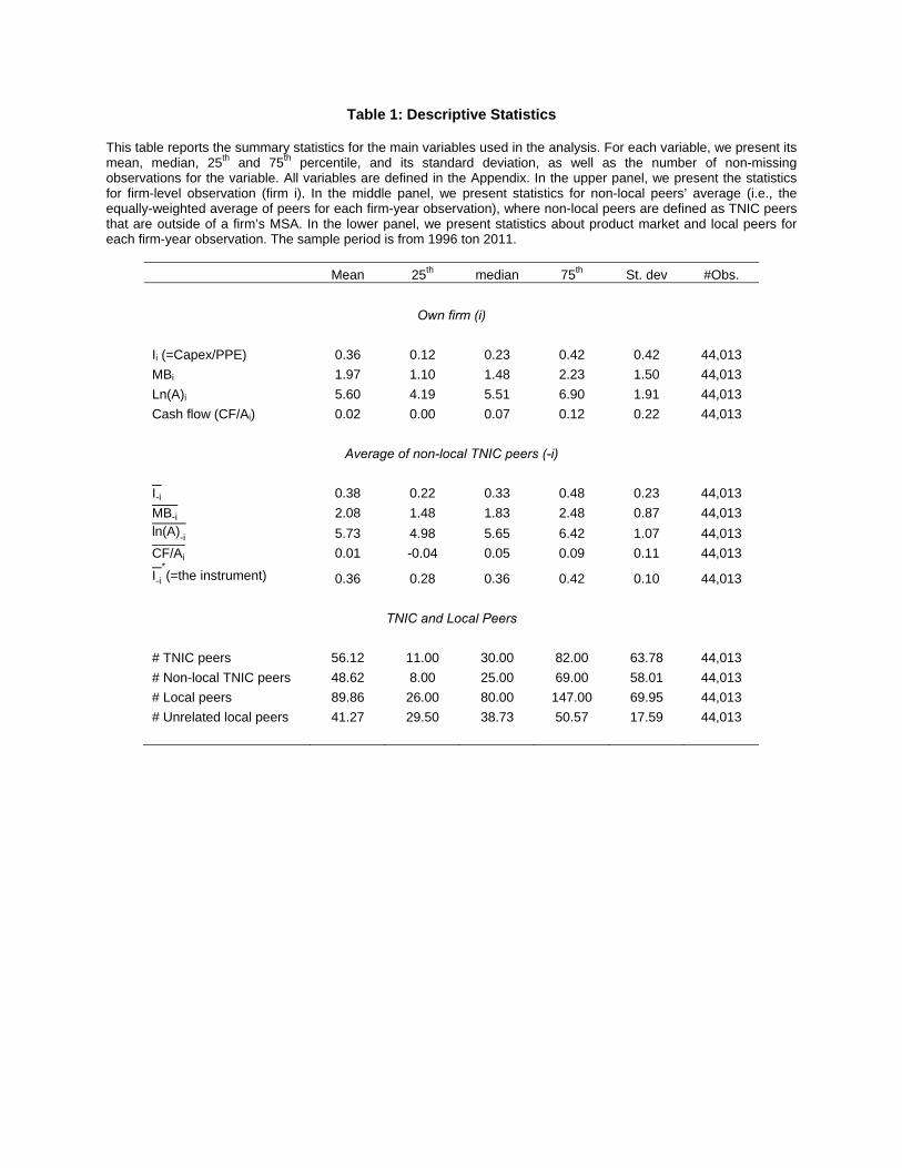
Table 1: Descriptive Statistics

This table reports the summary statistics for the main variables used in the analysis. For each variable, we present its mean, median, 25th and 75th percentile, and its standard deviation, as well as the number of non-missing observations for the variable. All variables are defined in the Appendix. In the upper panel, we present the statistics for firm-level observation (firm i). In the middle panel, we present statistics for non-local peers’ average (i.e., the equally-weighted average of peers for each firm-year observation), where non-local peers are defined as TNIC peers that are outside of a firm’s MSA. In the lower panel, we present statistics about product market and local peers for each firm-year observation. The sample period is from 1996 ton 2011.

Mean 25th median 75th St. dev #Obs.

Own firm (i)

Ii (=Capex/PPE) 0.36 0.12 0.23 0.42 0.42 44,013

MBi 1.97 1.10 1.48 2.23 1.50 44,013

Ln(A)i 5.60 4.19 5.51 6.90 1.91 44,013

Cash flow (CF/Ai) 0.02 0.00 0.07 0.12 0.22 44,013

Average of non-local TNIC peers (-i)

I-i 0.38 0.22 0.33 0.48 0.23 44,013

MB-i 2.08 1.48 1.83 2.48 0.87 44,013 ln(A)-i 5.73 4.98 5.65 6.42 1.07 44,013

CF/Ai 0.01 -0.04 0.05 0.09 0.11 44,013

I-i*(=the instrument) 0.36 0.28 0.36 0.42 0.10 44,013

TNIC and Local Peers

# TNIC peers 56.12 11.00 30.00 82.00 63.78 44,013

# Non-local TNIC peers 48.62 8.00 25.00 69.00 58.01 44,013

# Local peers 89.86 26.00 80.00 147.00 69.95 44,013

# Unrelated local peers 41.27 29.50 38.73 50.57 17.59 44,013

Table 2: The Influence of Peers’ Investment: Main Results

This table presents panel OLS and Instrumental Variables (IV) estimations of the baseline investment specification (specification (11) in the text). The dependent variable is investment of firm i, defined as capital expenditures divided by lagged property, plant, and equipment (Ii). The independent variables include average peers’ characteristics (market-to-book ratio, size, and cash flows) and investment, as well as firms’ own characteristics. For each firm-year observation, peers’ averages are constructed as equally-weighted averages of all non-local TNIC peers. The subscript –i refers to the average value of the variable across firm i’s peers. Column (1) reports the OLS estimates. Column (2) reports the first-stage estimates, and column (3) reports the second-stage estimates. The endogenous variable is the average investment of non-local TNIC peers. The instrument is the average investment of the local

MSA peers of non-local TNIC peers (I-i*). All specifications include Firm and MSA×Year fixed effects. All variables are

defined in the Appendix. To facilitate economic interpretation, all dependent variables are standardized to have a unit standard deviation. Standard errors are clustered by firm. We report t-statistics in parenthesis. Symbols *, **, and *** indicate statistical significance at the 10%, 5%, and 1% level, respectively.

Dependent Variable: Capex/PPE (Ii)

Specification: OLS IV

(1) (2) (3)

Peers’ Characteristics

I-i 0.046*** 0.037**

(10.41) (2.45)

MB-i 0.033*** 0.419*** 0.02

(6.79) (32.39) (1.46) ln(A)-i 0.002 -0.017* 0.003

(0.67) (-1.83) (0.82)

CF/Ai 0.008** 0.044*** 0.007*

(2.02) (4.37) (1.73)

Firm Characteristics

MBi 0.130*** 0.068*** 0.128***

(24.46) (12.25) (23.27)

Ln(A)i -0.084*** 0.01 -0.084***

(-6.44) (0.65) (-6.69)

CF/Ai 0.034*** 0.019*** 0.033***

(9.02) (3.46) (5.47)

Instrument

I-i* 0.113***

(12.48)

Firm Fixed Effects Yes Yes Yes

MSA×Year Fixed Effects Yes Yes Yes

#Obs. 44,013 44,013 44,013

Adj. R2 0.46 0.68 0.34

Table 3: Checking the Validity of the Instrument: Placebo Peers

This presents the results of 1,000 estimations a modified investment specification (specification (11) in the text) in which we change replace non-local product market peers by one randomly selected firm that is located in the same MSA as the original peer but operates in an unrelated product market, as described in section 4.B. Panel A reports descriptive statistics obtained across 1,000 first-stage estimates and their respective t-statistics, and panel B reports the corresponding second-stage estimates and their respective t-statistics.

mean sd p10 p25 p50 p75 p90 N

Panel A: First-stage estimates

Coefficient on I-i* 0.155 0.003 0.151 0.154 0.155 0.157 0.159 1,000

t-statistic 20.001 0.495 19.417 19.680 19.954 20.397 20.668 1,000

Panel B: Second-stage estimates

Coefficient on I-i -0.001 0.017 -0.021 -0.011 -0.001 0.010 0.022 1,000

t-statistic -0.032 0.997 -1.219 -0.670 -0.076 0.591 1.280 1,000

Table 4: Instrument Properties: Correlation with Fundamentals

This table presents results from panel OLS estimations, in which the dependent variable is the average investment of the local peers of non-local product market peers (I+-i) measured in year t. The independent variables include firm’s characteristics (displayed), average peers’ characteristics and investment (not-displayed). For each firm-year observation, peers’ averages are constructed as equally-weighted averages of all non-local TNIC peers. Both specifications include Firm and MSA×Year fixed effects. Column (3) and (4) further include FIC×Year fixed effects, where FIC is the Fixed Industry Classification (100) developed by Hoberg and Phillips (2015). In columns (1) and (3), the independent variable is also measured in year t, while in columns (2) and (4) they are measured with a one-year lead (i.e. in year t+1). All variables are defined in the Appendix. To facilitate economic interpretation, all dependent variables are standardized to have a unit standard deviation. Standard errors are clustered by firm. We report t-statistics in parenthesis. Symbols *, **, and *** indicate statistical significance at the 10%, 5%, and 1% level, respectively.

Dependent Variable: Local Capex/PPE (I-i*)

Specification: Contemp. one-year lead Contemp. one-year lead

(1) (2) (1) (2)

MBi 0.000 -0.001 0.000 -0.000

(0.77) (-1.19) (1.47) (-1.39)

Ln(A)i 0.001 0.001 0.000 0.001

(0.72) (1.02) (0.49) (1.11)

Cash flow (CF/Ai) -0.000 -0.001** -0.000 -0.000

(-0.87) (-2.02) (-0.78) (-1.48)

Peers' Characteristics Yes Yes Yes Yes

Peers' Investment (I-i) Yes Yes Yes Yes

Firm Fixed Effects Yes Yes Yes Yes

MSA×Year Fixed Effects Yes Yes Yes Yes

FIC×Year Fixed Effects No No Yes Yes

#Obs. 44,013 44,013 44,013 44,013

Adj. R2 0.77 0.74 0.81 0.79

Table 5: The Influence of Peers’ Investment: Robustness

This table presents panel Instrumental Variables (IV) estimations of various modifications of the baseline investment specification (specification (11) in the text). The dependent variable is investment of firm i, defined as capital expenditures divided by lagged property, plant, and equipment (Ii). The independent variables include average peers’ characteristics (market-to-book ratio, size, and cash flows) and investment, as well as firms’ own characteristics. For each firm-year observation, peers’ averages are constructed as equally-weighted averages of all non-local TNIC peers. The subscript –i refers to the average value of the variable across firm i’s peers. The endogenous variable is the average investment of non-local TNIC peers. The instrument is the average investment of the local MSA peers of non-local TNIC peers (I+-i). All specifications include Firm and MSA×Year fixed effects. For brevity we only report the estimated coefficient on peers’ average investment (I-i). Column (1) and (2) further include FIC×Year fixed effects, where FIC is the Fixed Industry Classification (100 or 300) developed by Hoberg and Phillips (2015). Column (3) includes additional peers- and firm-level controls (sales growth, PPE/assets, leverage, and cash/assets). Column (4) only use non-local peers that are located more than 300 miles away. Columns (5) and (6) compute peers’ weighted averages instead of equally-weighted averages, with weights based on sales and assets. Column (6) defines product market peers using the 3-digit Standard Industry Classification (SIC) definition. Columns (8) and (9) replace the dependent variables with the growth in PPE and the growth in assets. All variables are defined in the Appendix. To facilitate economic interpretation, all dependent variables are standardized to have a unit standard deviation. We report the t-statistic of the instrument from the first-stage estimation at the bottom of each column. Standard errors are clustered by firm. We report t-statistics in parenthesis. Symbols *, **, and *** indicate statistical significance at the 10%, 5%, and 1% level, respectively.

Dependent Variable: Capex/PPE (Ii) ΔPPE (Ii) ΔA(Ii)

Specification: FIC100 FIC300 Controls >300m w(sales) w(A) SIC

(1) (2) (3) (4) (5) (6) (7) (8) (9)

I-i 0.038*** 0.044*** 0.029** 0.021** 0.039*** 0.037*** 0.023*** 0.060* 0.052***

(2.60) (3.01) (1.97) (2.21) (3.58) (3.33) (2.65) (1.67) (4.06)

Peers Controls Yes Yes Yes Yes Yes Yes Yes Yes Yes

Firm Controls Yes Yes Yes Yes Yes Yes Yes Yes Yes

Firm Fixed Effects Yes Yes Yes Yes Yes Yes Yes Yes Yes

MSA×Year Fixed Effects Yes Yes Yes Yes Yes Yes Yes Yes Yes

Ind×Year Fixed Effects Yes Yes No No No No No No No

#Obs. 44,013 44,013 42,829 43,399 44,013 44,013 44,013 44,013 44,013

First-Stage t-statistic 10.68*** 11.25*** 12.31*** 11.68*** 11.51*** 13.93*** 14.23*** 6.95*** 11.97***

Table 6: Peer Effects in Corporate Investment: Learning vs. Strategic Channel This table presents panel Instrumental Variables (IV) estimations of the interaction investment specification (specification (12) in the text). The dependent variable is investment of firm i, defined as capital expenditures divided by lagged property, plant, and equipment (Ii). We consider eight different variables as proxies for the model key parameters (Δσ, ρ, ΔK, and h). We interact the average investment of non-local TNIC peers (I-i) and each other independent variable with two indicator variables identifying the lower (Dlow) and upper (Dhigh) half of each proxy variable distribution. We measure all proxies with one year lag, and assign firm-year observations into each group every year. The independent variables include average peers’ characteristics (market-to-book ratio, size, and cash flows) and investment, as well as firms’ own characteristics. For each firm-year observation, peers’ averages are constructed as equally-weighted averages of all non-local TNIC peers. The subscript –i refers to the average value of the variable across firm i’s peers. The endogenous variables are the interactions between the average investment of non-local TNIC peers and the two indicator variables. We instrument each interaction term with the interaction between the instrument (i.e., the

average investment of the local MSA peers of non-local TNIC peers (I-i*)) and each indicator variable. All specifications include Firm and MSA×Year fixed effects.

For brevity we only report the estimated coefficients on the interaction terms between peers’ average investment (I-i) and the indicator variables (Dlow and Dhigh). All variables are defined in the Appendix. To facilitate economic interpretation, all dependent variables are standardized to have a unit standard deviation. We report the F-statistic corresponding to a test of equality between I-i Dlow and I-i Dhigh, as well as the F-statistic corresponding to the first-stages Craag-Donald Wald test. Standard errors are clustered by firm. We report t-statistics in parenthesis. Symbols *, **, and *** indicate statistical significance at the 10%, 5%, and 1% level, respectively.

Dependent Variable: Capex/PPE (Ii)

Model's Parameter: Δσ ρ ΔK h

Proxy (to construct D): ΔVoli,-i ΔAgei,-i Similarityi,-i Co-Coveragei,-i Δln(PPE)i,-i Δln(A)i,-i HHI(k)i #Peersi

(1) (2) (3) (4) (5) (6) (7) (8)

I-i Dlow 0.031 0.087*** 0.095*** 0.074*** 0.104*** 0.110*** 0.024 0.065**

(1.21) (2.82) (2.54) (2.91) (3.78) (4.06) (0.56) (2.22)

I-i Dhigh 0.076*** 0.056 0.012 0.056*** 0.035 0.017 0.077*** 0.021

(2.82) (0.55) (0.23) (4.54) (1.18) (0.55) (2.87) (0.40)

Test coefficient F-Stat 6.32** 3.89** 5.26** 0.71 13.59*** 21.45*** 5.27** 3.45*

First-Stage F-Stat 245.03*** 200.44*** 163.51*** 188.51*** 212.78*** 208.64*** 184.93*** 157.34***

Peers Controls Yes Yes Yes Yes Yes Yes Yes Yes

Firm Controls Yes Yes Yes Yes Yes Yes Yes Yes

Firm Fixed Effects Yes Yes Yes Yes Yes Yes Yes Yes

MSA×Year Fixed Effects Yes Yes Yes Yes Yes Yes Yes Yes

#Obs. 44,013 44,013 44,013 44,013 44,013 44,013 44,013 44,013

Table 7: Blending with the Crowd and Strategic Complementarity This table presents panel Instrumental Variables (IV) estimations of the interaction investment specification (specification (12) in the text). The dependent variable is investment of firm i, defined as capital expenditures divided by lagged property, plant, and equipment (Ii). We interact the average investment of non-local TNIC peers (I-i) and each other independent variable with indicator variables identifying whether firms use relative performance evaluation in their CEO compensation contract (columns (1) and (2) and whether firms compete in strategic substitutes or complements (column (3)).The variable DRPE=0 is equal to one if firms do not use RPE while DRPE=1 is equal to one if firms use RPE. We assign firm-year observations into the two groups based on a proxy for RPE obtained by regressing (for each industry-year) CEO compensations on their firm’s lagged annual stock return and the lagged average stock return of their industry peers. We define that firms do not use RPE is the estimate on the peer returns is larger than zero. In column (1) we define peers using 2-digit SIC industries, and in column (2) we define peers using 3-digit SIC industries. The variable DSUBS is equal to one if firms have a negative value for the Competitive Strategy Measure (CSM), and DCOMP is equal to one if firms have a positive value for CSM. The independent variables include average peers’ characteristics (market-to-book ratio, size, and cash flows) and investment, as well as firms’ own characteristics. For each firm-year observation, peers’ averages are constructed as equally-weighted averages of all non-local TNIC peers. The subscript –i refers to the average value of the variable across firm i’s peers. The endogenous variables are the interactions between the average investment of non-local TNIC peers and the two indicator variables. We instrument each interaction term with the interaction between the instrument (i.e., the

average investment of the local MSA peers of non-local TNIC peers (I-i*)) and each indicator variable. All

specifications include Firm and MSA×Year fixed effects. For brevity we only report the estimated coefficients on the interaction terms between peers’ average investment (I-i) and the indicator variables. All variables are defined in the Appendix. To facilitate economic interpretation, all dependent variables are standardized to have a unit standard deviation. We report the F-statistic corresponding to a test of equality between coefficients, as well as the F-statistic corresponding to the first-stages Craag-Donald Wald test. Standard errors are clustered by firm. We report t-statistics in parenthesis. Symbols *, **, and *** indicate statistical significance at the 10%, 5%, and 1% level, respectively.

Dependent Variable: Capex/PPE

Proxy (to construct D): RPE (SIC2) RPE (SIC3) CSM (TNIC)

(1) (2) (3)

I-i DRPE=0 0.066*** 0.0075***

(2.68) (2.92)

I-i DRPE=1 0.031 0.046*

(1.27) (1.79)

I-i DSUBS 0.050**

(2.14)

I-i DCOMP 0.071***

(2.79)

Test coefficient F-Stat 1.85 1.91 1.14

First-Stage F-Stat 199.51*** 212.50*** 210.38***

Peers Controls Yes Yes Yes

Firm Controls Yes Yes Yes

Firm FE Yes Yes Yes

MSAxYear FE Yes Yes Yes

# Obs 44,013 44,013 44,013

Does Firm Investment Respond to Peers’ Investment?2017-5-24 · Electronic copy available at :...

Documents

Transcript of Does Firm Investment Respond to Peers’ Investment?2017-5-24 · Electronic copy available at :...