Docking study of matrix metalloproteinase inhibitors - Muni

MASARYK UNIVERSITYFACULTY OF SCIENCE

NATIONAL CENTRE FOR BIOMOLECULAR RESEARCH

Docking study of matrixmetalloproteinase inhibitors

BACHELOR THESIS

Jan Ryška

Brno, spring 2011

Declaration

Hereby I declare, that this paper is my original authorial work, whichI have worked out by my own. All sources, references and literatureused or excerpted during elaboration of this work are properly citedand listed in complete reference to the due source.

Jan Ryška

Supervisor: RNDr. Radka Svobodová Vareková, Ph.D.Consultant: MSc. Sushil Kumar Mishra

ii

Acknowledgement

I would like to acknowledge my supervisor RNDr. Radka SvobodováVareková, Ph.D. for her patient leadership and help throughout writ-ing of this thesis.

I would also like to thank my consultant MSc. Sushil Kumar Mish-ra for his valuable insights and advice on the topic, Mgr. MartinProkop, Ph.D. for implementation of parameters for metals in TRI-TON and all members of LCC for support.

iii

Keywords

docking, matrix metalloproteinase inhibitors, AutoDock, DOCK, zincparameters, structure-based drug design

iv

Contents

1 Introduction . . . . . . . . . . . . . . . . . . . . . . . . . . . . 12 Theory . . . . . . . . . . . . . . . . . . . . . . . . . . . . . . . 3

2.1 Matrix metalloproteinases . . . . . . . . . . . . . . . . . 32.1.1 Structure and function . . . . . . . . . . . . . . . 32.1.2 Active site . . . . . . . . . . . . . . . . . . . . . . 62.1.3 Inhibition . . . . . . . . . . . . . . . . . . . . . . 7

2.2 Molecular docking . . . . . . . . . . . . . . . . . . . . . 72.2.1 Search algorithms . . . . . . . . . . . . . . . . . . 102.2.2 Scoring function . . . . . . . . . . . . . . . . . . 13

3 Methods . . . . . . . . . . . . . . . . . . . . . . . . . . . . . . 153.1 Test set . . . . . . . . . . . . . . . . . . . . . . . . . . . . 153.2 Docking preparation . . . . . . . . . . . . . . . . . . . . 15

3.2.1 Ligand preparation . . . . . . . . . . . . . . . . . 153.2.2 Receptor preparation . . . . . . . . . . . . . . . . 16

3.3 Docking software . . . . . . . . . . . . . . . . . . . . . . 173.3.1 AutoDock 3 . . . . . . . . . . . . . . . . . . . . . 173.3.2 AutoDock 4 . . . . . . . . . . . . . . . . . . . . . 193.3.3 AutoDock Vina . . . . . . . . . . . . . . . . . . . 203.3.4 UCSF DOCK 6.4 . . . . . . . . . . . . . . . . . . 20

3.4 Analysis of results . . . . . . . . . . . . . . . . . . . . . . 213.4.1 RMSD . . . . . . . . . . . . . . . . . . . . . . . . 213.4.2 Binding score . . . . . . . . . . . . . . . . . . . . 22

4 Results and discussion . . . . . . . . . . . . . . . . . . . . . . 244.1 Software comparison . . . . . . . . . . . . . . . . . . . . 24

4.1.1 Geometry prediction . . . . . . . . . . . . . . . . 244.1.2 Binding affinity prediction . . . . . . . . . . . . . 26

4.2 Publication outputs . . . . . . . . . . . . . . . . . . . . . 285 Conclusions . . . . . . . . . . . . . . . . . . . . . . . . . . . . 296 Summary . . . . . . . . . . . . . . . . . . . . . . . . . . . . . . 307 Souhrn . . . . . . . . . . . . . . . . . . . . . . . . . . . . . . . 318 Appendices . . . . . . . . . . . . . . . . . . . . . . . . . . . . 32

8.1 Docking results by receptor . . . . . . . . . . . . . . . . 328.2 List of complexes ordered by binding affinity . . . . . . 388.3 Contents of the attached CD . . . . . . . . . . . . . . . . 39

Bibliography . . . . . . . . . . . . . . . . . . . . . . . . . . . . . . 40

v

1 Introduction

Computational chemistry [1] is a branch of classical chemistry whichuses principles from computer science to solve chemical problems.Both fields are based on the same theoretical grounds, but they arealso different in many ways.

Cooperation of computational and classical chemistry is bene-ficial for both fields. The computational methods and mathemati-cal descriptions of chemical systems are developed based on resultsfrom classical chemistry. On the other hand, computational chem-istry can be used to predict experimental results, so the researcherscan prepare more efficient and targeted experiments. It can also beused to predict properties of molecules, which are too unstable towork with or too difficult or expensive to prepare or purchase.

Molecular docking [2–4] is an in silico computational techniqueused to predict conformation and binding affinity of intermolecularcomplexes based on the three-dimensional structures of individualmolecules. This method is widely used in the field of structure-baseddrug design, in which researchers try to find compounds, which willform a stable intermolecular complex with a target protein. The tar-get protein is usually known to play a vital role in a pathological pro-cess, so finding a potent inhibitor is crucial in disruption of its func-tion. Initial screening of possibly millions of compounds in a labora-tory conditions is often too expensive and time-consuming processto be feasible and thus fast molecular docking methods are used toeliminate unlikely candidates.

Like many methods in the field of computational chemistry, molec-ular docking uses a number of approximations to reduce a time re-quired for each simulation. As it has many applications, we need tobe aware of its accuracy and possible limitations.

One of the identified challenges is how docking software handlesnon-standard atoms, such as metal atoms [5]. While docking pro-grams often employ chemical system descriptions based on molec-ular mechanics, majority of them requires parameters for individualatom types. An extensive effort has been put into optimization ofthese parameters for common atom types, such as atom types of car-bon and oxygen. However, parameters for non-standard atoms are

1

1. INTRODUCTION

usually based on a much smaller data sets, or entirely missing in thesoftware.

In this thesis, we present an overview of molecular docking meth-ods as well as comparison of several docking software. As a test set,we used a family of matrix metalloproteinases [6], where interactionof a ligand with a metal ion is crucial in the process of complex for-mation.

2

2 Theory

This chapter is divided into two parts. First section introduces matrixmetalloproteinases, biologically important proteins that are in focusof this thesis.

Second section provides overview of the theory behind moleculardocking, describing several algorithms and programs employed tosolve the docking problem.

2.1 Matrix metalloproteinases

Matrix metalloproteinases (MMPs) [6] are a family of zinc-dependent,calcium-containing endopeptidases.

The MMPs belong to a larger family of proteases known as met-zincin superfamily [7]. The research in the field of MMPs was initi-ated in 1962, when Gross and Lapiere [8] reported the discovery of acollagenolytic enzyme involved in resorbing amphibian tadpole tailsduring metamorphosis. The enzyme was named interstitial collage-nase (MMP-1) and became the first member of the MMP family. Sincethen, many other members of this family were found in vertebrates,including human, as well as in invertebrates and plants.

2.1.1 Structure and function

MMPs can be divided into eight groups based on their domain struc-ture [9]. Three common homologous domains include the N-terminalpro-peptide, the catalytic domain and the hemopexin-like C-terminaldomain, which is linked to the catalytic domain by a flexible hingeregion. Many MMPs also contain one or more specific structural fea-tures, as shown in Figure 2.1.

Cysteine switch

MMPs are synthesized in the form of inactive zymogen. In this form,conserved cysteine residue in the pro-peptide domain interacts withthe zinc atom in the active site and prevents binding and cleavageof a substrate. In most MMPs, this particular cysteine is present in

3

2. THEORY

Figure 2.1: Domain structure of MMPs. Meaning of the importantabbreviations: Pre – signal peptide; Pro – pro-peptide domain; Fi –fibronectin-like repeats; Fu – recognition motif for furin-like serineproteases; Vn – vitronectin-like inserts [9].

4

2. THEORY

the conserved sequence PRCGxPD. The cleavage of the pro-peptidedomain is therefore crucial in the mechanism of MMP activation, socalled cysteine switch [10].

Upon release of the proenzyme from the cell, changes in the proen-zyme conformation or other proteases may open the cysteine switchand trigger proMMP activation. The pro-peptide domain is subse-quently removed in an autocatalytical manner or by proteases. Other,already active MMPs are also capable of proMMP activation.

Biological function

MMPs perform a variety of roles in living organisms. They are re-sponsible for the tissue remodeling and degradation of many extra-cellular matrix (ECM) proteins, including collagens, elastins, gelatin,matrix glycoproteins and proteoglycan [6]. More recently, it has alsobeen recognized that they cleave many other peptides and proteinsand perform other functions that may be independent of proteolyticactivity [11].

Physiological processes where MMPs are involved include angio-genesis (formation of new blood vessels), apoptosis (process of pro-grammed cell death), bone modeling or wound healing.

Role in pathological processes

Under normal physiological conditions, level of MMP expressionand activity is very low. Transcription of these enzymes is tightly reg-ulated by cytokines or growth factors, including transforming growthfactors, interleukins (IL-1, IL-4, IL-6) or tumor necrosis factor alpha(TNFα) [12]. Post-transcriptionally, MMP activity is controlled by in-teraction between zinc-containing catalytic site and N-terminal pro-peptide domain.

When this balance between MMPs and their natural inhibitorsis shifted towards enzyme expression and activity, increased tissuedegradation occurs. Increased levels of MMP expression have beenshown to be involved in a large number of pathological conditions,such as arthritis, Alzheimer’s disease, cardiovascular disease, as wellas cancer [6]. MMPs have now been therefore considered importantpharmaceutical targets and extensive effort have been put into de-

5

2. THEORY

sign of potential drugs based on MMP inhibition [13, 14].

2.1.2 Active site

The active site of MMPs features two distinct regions [6]. First oneis a groove centered on the catalytic zinc. Second one is a S1’ speci-ficity site, which varies among different members of a family and isimportant for substrate (or inhibitor) selectivity. The volume of thisS1’ subsite varies highly from a small hydrophobic pocket of MMP-7to a very large site in MMP-8.

An example illustrating the protein-ligand interactions occurringin the active site is presented in fig. 2.2.

2.67

2.99

2.73

3.22

3.14

CB CG1

CG2

N35

O48 C34

O47

O27

COM

CD1

CE1

C20

CD2

CE2 C17

N11

CY CZ

CE

CD

C5

S4

O33

O32

CA

CC

N1

CE1

NE2

CD2

ND1

CG

CB C

O CA

N

ZN

CG

CD2 CD1

CB

C

O

CA

N

C

O

CA

CB

N

CE1

NE2

CD2

ND1

CG

CB

C

O

CA

N CE1

NE2

CD2

ND1

CG

CB

C O

CA N

Asn 80(A)

Ser 139(A)

Pro 138(A)

Tyr 140(A)

His 83(A)

Cgs 173(A)

His 118(A)

ZN 170(A)

Leu 81(A) Ala 82(A)

His 122(A)His 128(A)

Figure 2.2: Interaction diagram of MMP-1/CGS complex (PDB ID:3AYK) generated by LIGPLOT [15]. Note the group chelating thezinc, hydrogen bonds (green) and hydrophobic contacts (orange).

6

2. THEORY

2.1.3 Inhibition

Binding affinity

The strength of interaction between receptor protein and ligand isvery important (but not the only one) criterion to distinguish potentinhibitors (i.e. potential drugs) from the non-binding compounds.

This attractive force between protein and ligand is called bindingaffinity. It is influenced by non-covalent interactions, such as hydro-gen bonding, electrostatic or van der Waals interactions.

MMP Inhibitors

As mentioned earlier, MMPs are promising pharmaceutical targets,especially for cancer therapy. Large number of both synthetic andnatural inhibitors have been identified and tested in clinical trials,but so far with only limited success.

While many of these compounds showed cytostatic or anti-angio-genic activity, discovered side effects or low specificity leading to ex-cessive inhibition of MMPs not involved in the particular patholog-ical process led to disappointing results [16]. Current effort is nowfocused on computer-aided design of more specific inhibitors basedon knowledge of three-dimensional structure of many MMPs [17].

The requirements [6] for a compound to be a potent MMP in-hibitor are following: a) a functional group capable of chelation ofcatalytic zinc(II) ion [e.g. carboxylate (COO−), thiolate (S−) or hy-droxamate (CONH-O−)]; b) one or more functional groups capableof interacting with enzyme backbone via hydrogen bonds; c) at leastone functional group, which will undergo van der Waals interactionswith the protein subsites.

2.2 Molecular docking

With the rapid increase in computational power, in silico methodsbecame widely used in the fields of structural molecular biology andstructure-based drug design. Molecular docking [2–4] is one of thesecomputational techniques.

Docking is a method which predicts preferred orientation of one

7

2. THEORY

molecule to the second when they bind to form a stable complex.In the field of drug design, first molecule is usually protein and thesecond one is a small organic molecule, potential drug candidate.Knowledge of preferred orientation of ligand and protein can thenbe used to predict binding affinity, thus discriminating high-affinitydrug candidates from the low-affinity compounds.

As a well established technique, certain terms are commonly usedin the field. A brief overview of terminology is presented in Table 2.1.

Lock-and-key analogy

Molecular docking is sometimes described as a problem of lock-and-key, where one is interested in finding the correct orientation of akey (ligand) that will open the lock (protein). While this analogy issimple to understand, it does not account for inherent flexibility ofboth molecules which is why more appropriate term hand-in-gloveis sometimes used.

Term Meaning

Receptor or hostor lock

The "receiving" molecule, commonly a protein

Ligand or guestor key

The complementary molecule binding to a re-ceptor, often a small organic molecule

Binding mode Relative position of the ligand to the receptorPose A candidate binding modeScoring Evaluation of a particular pose based on a

number and strength of favorable intermolec-ular interactions

Ranking Classification of ligands based on the pre-dicted binding affinity / binding score

Table 2.1: Docking terminology.

8

2. THEORY

Rigid-body docking vs. flexible docking

The docking problem involves many degrees of freedom [18]. Thereare three translational and three rotational degrees of freedom foreach molecule as well as the conformational degrees of freedom forboth molecules.

The simplest approach to docking is to take into account onlytranslational and rotational degrees of freedom and treat both recep-tor and ligand as rigid objects. This approach is known as rigid-bodydocking [18]. It depends from case to case, whether this approxima-tion is accurate enough or not.

If there are significant conformational changes within the molecu-les during the complex formation, this approach is inadequate. How-ever, generation and scoring of all possible conformations is pro-hibitively expensive in computer time.

Flexible docking algorithms [19] must therefore take into consid-eration only a selected subset of possible conformational changes.Today with continual increase in computational resources, ligandsare often considered flexible and depending on required accuracy,flexibility of amino acid side chains in the vicinity of active site maybe considered as well.

Explicit vs. implicit solvent

Another division can be made based on how docking software treatseffect of solvent. There are two ways we can include solvent (usuallywater) and its interaction with protein in our simulation.

It is possible to include individual water molecules in our cal-culations [20]. The simplest model treats water molecules as rigidand relies only on non-bonded interactions. Coulomb’s Law is usedto calculate electrostatic interactions and repulsion forces are treatedby Lennard-Jones potential. The accuracy of this approach can be en-hanced by addition of interaction sites to each molecule, but the com-putational cost of including water molecules, thus greatly increasingthe number of atoms, in the system is expensive. While docking sim-ulations need to be as fast as possible, following approach is com-monly used.

Implicit solvation [21] (sometimes referred to as continuum sol-

9

2. THEORY

vation) is a method, which approximates behavior of many highlydynamic solvent molecules by a continuous medium. In liquids, thepotential of mean force can be used to approximate behavior of indi-vidual molecules. This approach is less computationally demandingand is commonly used in molecular dynamics and other applicationsof molecular mechanics.

2.2.1 Search algorithms

The search space which the docking software should take into ac-count, theoretically consists of every possible conformation and ori-entation of the receptor and ligand. While it is impossible to exhaus-tively explore this search space, efficient search algorithm is able toexplore its large portion and identify global extrema (i.e. minima inthe energy corresponding to the preferred conformations) [22].

The docking problem can be handled manually with help of in-teractive computer graphics. This solution may work, if we have agood idea of the binding mode of a similar ligand. Automatic soft-ware will be however less biased than a human and will considermany more possibilities in much shorter time frame. Overview ofthe three commonly used automatic docking algorithms is presentedin the following paragraphs.

Shape complementarity

As the name suggests, software using this geometry-based algorithmwill try to find the preferred complex conformation based on degreeof shape complementarity [18]. Good example is an algorithm usedin one of the docking programs DOCK [23].

The algorithm first generates a "negative image" of the bindingsite from the molecular surface of the receptor. This image consistsof a number of overlapping spheres of varying radii. Each spheretouches the receptor surface at only two points. Ligand atoms arethen matched to the sphere centers to find matching sets (cliques) inwhich all the distances between the ligand atoms in the set are equalto the corresponding sphere center – sphere center distances with aspecified tolerance. The ligand can then be oriented in the bindingsite by performing a least-squares fit of the atoms to the sphere cen-

10

2. THEORY

ters.After checking the generated conformations for unfavorable steric

clashes, a score is calculated for the particular conformation. The top-scoring conformations are stored for further analysis.

Monte Carlo methods

Monte Carlo methods [24] refer to a simulation which uses com-puter algorithm dependent on a series of (pseudo)random numbers.Its name, derived from the famous Monacco casino, emphasizes in-fluence of randomness in the method. The basic algorithm can bedescribed in the following steps:

1. Randomly generate starting conformation C1.

2. Calculate energy E1 (e.g. using molecular mechanics).

3. Generate new conformation C2. At each iteration, this confor-mation is produced by a random change of the internal confor-mation of the ligand (i.e. rotation about a bond in the ligandby random degree) or by rotation or translation of the wholemolecule.

4. Calculate E2.

5. Apply so called Metropolis criterion to determine whether theC2 conformation is an improvement over starting conforma-tion C1. Description of the Metropolis criterion:

(a) If the difference between energy of the resulting confor-mation and the energy of starting conformation,

∆E = E2 − E1, (2.1)

is negative (i.e. the energy of the resulting conformationis lower), then the resulting conformation is accepted andstored as C1.

(b) If ∆E is positive, however, a (pseudo)random number be-tween 0 and 1, 0 < R < 1, is generated. The C2 conforma-tion is in this case accepted only if the following condition

11

2. THEORY

is true:e−∆E/T > R. (2.2)

Parameter T introduced in this equation denotes tempera-ture-like quantity used to control the acceptance probabil-ity of energetically unfavorable states. As it has the samecourse as a temperature function, higher values of this pa-rameter allow high-energy states to be considered.

(c) Ife−∆E/T < R, (2.3)

the resulting conformation C2 is refused.

6. Repeat steps 3-5.

While Monte Carlo is a stochastic method, it is not guaranteed tofind optimal complex conformation. Severity of the implications forthe docking has not been firmly established, but various versions ofMonte Carlo approach have been implemented in common dockingalgorithms.

Genetic algorithms

Genetic algorithms [25] are search methods that mimic the process ofevolution by incorporation of techniques inspired by natural evolu-tion, such as inheritance, mutation or crossover.

In genetic algorithm, an initial population of one-dimensional str-ings (called chromosomes), which encode candidate solutions (indi-viduals) evolves toward better solutions. In case of a molecular dock-ing, each individual may represent one possible system configura-tion and each string may contain information about its conformation(e.g. values of angles of rotatable bonds).

At the beginning, initial population is randomly generated. In thenext step, a subset of the initial population is chosen (based on resultsof the fitness function, which evaluates the quality of a particular in-dividual). This subset is subsequently used to produce next genera-tion. New generations are produced until a certain number of stepsis performed or until a required level of fitness is reached.

One example of genetic algorithm which was used in this work isLamarckian Genetic Algorithm (LGA).

12

2. THEORY

Lamarckian Genetic Algorithm

LGA is hybrid genetic algorithm named after Jean-Baptiste Lamarck(1744-1829), a French soldier and academic, who proposed an idea,that organisms can pass on characteristics that they learned or ac-quired during their life to their offspring [26]. While this idea con-tradicts Mendelian genetics and was later disproved, its implemen-tation into genetic algorithm may lead to more accurate docking re-sults.

Genome is in LGA represented by floating point genes (unlikeclassical genetic algorithms, which use binary representation), eachof which encodes one state variable describing molecular position,orientation and conformation.

2.2.2 Scoring function

Search algorithms are able to quickly generate large number of pos-sible conformations. The "quality" of these possible solutions need tobe compared, so that best binding modes can be selected. This is thepurpose of a scoring function used in docking software [27].

Many of the scoring functions in common use attempt to ap-proximate the binding free energy (or other energy-like quantity) forthe ligand binding to the receptor; a low (negative) energy indicatesstable system and thus a likely receptor-ligand binding interaction.While many ways to predict free energies of binding exist, most ofthem are too computationally expensive to be of use in the field ofmolecular docking. Faster, more approximate scoring functions tendto be used.

These simplified scoring function usually assume that the bind-ing free energy can be written as a sum of several additive compo-nents representing various contributions to the binding free energy.An equation of this kind would have the following contributions:

∆Gbind = ∆Gsolvent + ∆Gconf + ∆Gint + ∆Grot + ∆Gt/r + ∆Gvib (2.4)

∆Gsolvent represents contributions of solvent effects, which arise fromthe interaction of the solvent and ligand, receptor and the intermolec-ular complex. ∆Gconf arises from the conformational changes in bothprotein and especially more flexible ligand. ∆Gint stands for the free

13

2. THEORY

energy of specific protein-ligand interactions. ∆Grot is the free energyloss caused by freezing of the internal rotations. ∆Gr/t is a change inrotational and translational free energy due to association of recep-tor and ligand, forming a single body and ∆Gvib corresponds to freeenergy changes in vibrational modes. More details on each term canbe found for example in [18] or [28].

14

3 Methods

Procedure, which was used for docking of MMP/ligand complexesand analysis of results is described in this chapter. Auxiliary softwareused in docking preparation and evaluation is reported and moredetails on algorithms and parameters employed by tested dockingsoftware are given.

3.1 Test set

Test set used in this thesis consists of 38 complexes of MMPs and var-ious ligands. Three-dimensional coordinates of MMP/ligand struc-tures were obtained from RCSB Protein Data Bank [29]. The struc-tures were experimentally determined by X-ray crystallography orNMR spectroscopy.

Complexes of following MMPs were used: MMP-1, -3, -7, -9, -12,-13 and -20. These were reported in complexes with ligands varyingin size (the smallest ligand contains only 5 heavy atoms, the largest33) and functional groups they contain.

3.2 Docking preparation

At the beginning of a docking procedure, water and possibly othersuperfluous molecules (e.g. artifacts of crystallization process) are re-moved from the structure and three-dimensional coordinates of re-ceptor and ligand are divided into separate files.

Each receptor and ligand is subsequently prepared for dockingin several steps. This section describes steps in a docking procedurethat are universal for all tested software.

3.2.1 Ligand preparation

Geometry and partial charges of all ligands were optimized. For thegeometry optimization, we used Hartree-Fock method using 6-31G*basis set, as implemented in Gaussian 03 [30].

15

3. METHODS

Partial charges were calculated by antechamber [31]. Antecham-ber is a program in the software suite Amber [32], which can be usedfor atom type assignment, conversion between formats as well asgeneration of charges by several implemented methods.

Docking programs are usually adjusted to work better with par-tial charges calculated by certain method. Because of this fact, weused different charge calculation methods for AutoDock and DOCK,respectively. These are mentioned in sections 3.3.1 and 3.3.4.

The process of ligand preparation can be summarized in thesesteps:

1. Add all the hydrogen atoms using UCSF Chimera [33]. Hydro-gen atoms are important for correct geometry optimization andcalculation of partial charges.

2. Convert the ligand file to a .com format by Open Babel [34].This file contains three-dimensional Cartesian coordinates ofeach ligand atom, as well as commands recognized by Gaus-sian.

3. Run geometry optimization procedure in Gaussian using pre-viously prepared .com file as input. Output file will contain lig-and with optimized geometry.

4. Assign partial charges by antechamber.

3.2.2 Receptor preparation

The receptor structures were checked and eventually corrected bytleap (using ff99SB force field), another program in Amber suite usedto prepare input files for simulation programs.

These corrections included addition of missing atoms, such as N-and C-terminal atoms or missing hydrogens. Further manipulationof receptor structure then depends on a particular docking softwareused.

16

3. METHODS

3.3 Docking software

In this section, we present detailed information about tested dock-ing software, including software-specific steps in receptor and ligandpreparation as well as parameters used in docking simulations.

3.3.1 AutoDock 3

AutoDock 3 [35] is an automatic docking software introduced in1998. While preceding versions of AutoDock used the Metropolismethod described in 2.2.1 to search conformational space, version 3introduced implementation of Lamarckian Genetic Algorithm (LGA).

It also uses enhanced scoring function [36] based on the principlesof QSAR (quantitative structure-activity relationship), which was pa-rameterized using a large number of protein-ligand complexes.

The AutoDock actually consists of two main programs: AutoDockand AutoGrid. AutoDock performs the actual docking of the ligandto a pre-calculated grids describing target protein. AutoGrid, whichis run prior to AutoDock, calculates these grids.

AutoGrid

AutoGrid pre-calculates grid maps of interaction energies betweenmacromolecule, such as protein, and various atom types, such asaliphatic carbons or hydrogen-bonding oxygens.

Doing this pre-calculation saves the time required for the dock-ing, as it reduces the order of complexity of a problem from N2 to N ,with N being the number of interacting atoms.

Ligand preparation

RESP charges were added to the ligand file by antechamber. Furthersteps in ligand and receptor preparation as well as preparation ofdocking simulation were carried out in the in-house developed in-teractive graphics software TRITON [37].

In the next step, the non-polar hydrogens (i.e. the hydrogens inmethyl and methylene groups) were merged. This step is necessarybecause AutoDock uses United Atom model [18].

17

3. METHODS

United Atom model

AutoDock uses United Atom model to simplify the system and toreduce the number of degrees of freedom. In this model, non-polarhydrogens are deleted and their charges are merged into the carbonatom which they bind. This way methyl and methylene groups ef-fectively form a single interaction center.

Another parameter that affects accuracy and time required for thesimulation is the flexibility allowed to the ligand. This flexibility isexpressed in the number of rotatable bonds.

While taking into account full flexibility of a ligand is desirable,as it is possible to access larger portion of the conformational spacethis way, ligands with too many rotatable bonds may present a chal-lenge to the docking software, resulting in increased time required tocomplete the simulation.

In our case, flexibility of ligands was not restricted. That is, allbonds excluding those inherently non-rotatable (e.g. double or aro-matic bonds), were considered freely rotatable.

Receptor preparation

The charges on receptor atoms were assigned using the Kollmanunited atoms force field (ff84) [38] as recommended by AutoDockauthors. The charges on metal atoms, namely calcium (+2.0 e) andzinc (+0.95 e), were added manually. The non-polar hydrogens weremerged and solvation parameters were set automatically by TRI-TON.

Zinc parameters

Catalytic zinc plays a crucial role in the binding of a ligand to the ac-tive site. Zinc parameters are therefore very important for the correctconformation prediction.

For this thesis, results from parametrization study [39] summa-rized in Table 3.1 were used.

18

3. METHODS

Parameter Charge Atom radius Well depthValue +0.95 e 0.87 Å 0.35 kcal/mol

Table 3.1: Values of zinc parameters.

Specifically for this work, parameters for metal atoms and capa-bility of conveniently changing atom radii and well depth were im-plemented in TRITON.

Docking preparation

When we have prepared receptor and ligand input files, it is neces-sary to set up parameters used for actual docking simulation such assearch algorithm, search exhaustiveness or location of input files.

Search space definition

Docking software requires definition of the search space. While weknow the location of an active site, we can reduce the size of thesearch space to a box enclosing the binding site.

In our case, each box was chosen to be centered on a catalytic zincand its dimensions were proportional to the ligand size, so the ligandcould freely move and rotate in the box during simulation.

LGA was used as a search algorithm and a maximum number of2.5 . 106 energy evaluations was set. One hundred docking runs wereperformed and the best scoring conformations were saved for analy-sis. The rest of the parameters was left at default values.

3.3.2 AutoDock 4

Although AutoDock 4 [40] has several new features and improve-ments over AutoDock 3, such as an enhanced scoring function, thedocking procedure itself remains very similar. Only notable excep-tion is a fact that it uses different atom types, which were set auto-matically by TRITON.

Concerning catalytic zinc, the same parameter set as in AutoDock 3was used, as there is currently not a similar parametrization study

19

3. METHODS

focused on AutoDock 4 known to us.

3.3.3 AutoDock Vina

AutoDock Vina [41] is the newest member of AutoDock suite intro-duced in 2010. It has been developed by Dr. Oleg Trott in the Molec-ular Graphics Lab at The Scripps Research Institute.

It differs from previous versions in many regards, one of them be-ing user-friendliness. Only three-dimensional structures of molecules(with polar hydrogens only, as AutoDock Vina still uses United Atommodel) and a box definition of a search space is required. Partialcharges, solvation parameters or pre-calculated interaction energygrids are not necessary for the simulation.

Unlike previous versions, it does not provide the user with achoice of search algorithm, instead it uses Iterated Local search globaloptimizer. In this algorithm, steps consisting of mutation and sub-sequent local optimization are performed, with each step being ac-cepted according to the Metropolis criterion. Details on this algo-rithm as well as on the scoring function used by AutoDock Vina canbe found in the original paper [41].

The preparation of receptor and ligand structures was performedusing AutoDock Tools [42], interactive graphics software distributedwith AutoDock.

3.3.4 UCSF DOCK 6.4

UCSF DOCK [23] is a docking software which uses geometry-basedsearch algorithm described in 2.2.1.

For the scoring function, we decided to use original DOCK scoreas well as GBSA (Generalized Born/surface area) method [43], whichis more computationally expensive, for re-scoring of the best confor-mations.

Ligand and receptor preparation

Both ligands and proteins were prepared for docking using UCSFChimera. This interactive graphics software includes a set of tools

20

3. METHODS

for convenient preparation of molecules under the procedure DockPrep.

It automatically carries out all necessary steps (deletion of sol-vent molecules, adding hydrogens, charge assignment) and writesthe output into a file in Mol2 format. The charges used in DOCKwere calculated by AM1-BCC method [44].

Sphere generation

Spheres required by a DOCK algorithm were generated using sph-gen [23] program, which is also provided with DOCK. As sphgencreates negative image of the protein, its procedure needs informa-tion about receptor surface. First step in the sphere set generationwas to prepare a file containing only receptor molecule without anyhydrogens.

This file was used as input for the program dms [45], which cal-culated surface of the receptor and saved it in .ms file format. Sphgensubsequently used .ms file for the actual sphere generation.

Similar to AutoDock, as we know the location of active site, wecan significantly narrow down the search space. In DOCK, this isachieved by creation of the box (with the same center and dimen-sions as in AutoDock ) around the binding site, as well as selectingthe spheres, which will be used in the docking procedure. In our case,only spheres in the 10 Å radius from the original ligand conforma-tion were considered and selected with the sphereselector utility.

3.4 Analysis of results

Two commonly used criteria were utilized for assessment of dockingsoftware accuracy.

3.4.1 RMSD

The first way to evaluate quality of a docked pose is to compare itsgeometry relative to the original experimental structure.

Difference between two conformations (or any three-dimensionalstructures) is often measured by computing root-mean square devi-ation (RMSD) [46].

21

3. METHODS

RMSD can be calculated using formula

RMSD =

√√√√ 1

N

N∑i=1

δ2i , (3.1)

where N is the total number of atoms in the molecule and δ is adistance between each pair of corresponding atoms.

Concerning current docking software accuracy, the RMSD valueof 2 Å is commonly used as a cutoff value. Poses closer to the exper-imentally determined structure (i.e. with RMSD lower than 2 Å) aregenerally considered sound.

RMSD for heavy atoms was calculated using RMSD Tool pluginimplemented in an interactive graphics software VMD [47].

3.4.2 Binding score

Accuracy of a scoring function was measured by a comparison ofpredicted binding score of a ligand with experimental value of freeenergy of binding.

While scoring functions employed in docking software tend touse various approximations to enhance their speed, their accuracy isnot on a level of more computationally expensive methods. To pro-vide a context, standard error of AutoDock 4 was estimated to bearound 2.5 kcal/mol [48].

In comparing binding energies predicted by docking softwarewith experimentally determined values, two criteria are commonlyconsidered.

First one is comparison of absolute values of energy, therefore ac-curacy of binding energy prediction. On the other hand, in the fieldof drug design, researchers are often more interested in comparinginhibitor potency relative to each other. For this purpose, dockingsoftware should ideally be able to rank the ligands from the most tothe least potent (predict the correct binding trend), even if the abso-lute values of binding energy are not accurate. Two correlation co-efficients are commonly used [49] to quantify relationship betweenactual and predicted biding trend.

22

3. METHODS

Pearson’s correlation coefficient

The Pearson product-moment correlation coefficient [50] is a mea-sure of correlation between variables X and Y. It is defined as thecovariance of the two variables divided by the product of their stan-dard deviations:

ρX,Y =cov(X, Y )

σXσY=E[(X − µX)(Y − µY )]

σXσY. (3.2)

The above formula defines the population correlation coefficientρ. If we substitute the covariances and variances based on a sample,we get sample correlation coefficient r:

r =

∑ni=1(Xi − X)(Yi − Y )√∑n

i=1(Xi − X)2√∑n

i=1(Yi − Y )2. (3.3)

The Pearson’s correlation coefficient ranges from -1 to +1. A valueof +1 means that all data points lie on a line for which Y increases asX increases. A value of -1 implies that all data points lie on a line forwhich Y decreases as X increases. A value of 0 implies that there isno linear relationship between X and Y.

The higher the Pearson’s coefficient value between experimentaland predicted values of binding energy, the better is the ability ofdocking software to correctly determine the order of potency of theligands.

Spearman’s rank correlation coefficient

The Spearman’s rank correlation coefficient [51] is defined as thePearson’s correlation coefficient between ranked values. The valuesXi, Yi are first converted to ranks xi, yi and ρs is computed from these:

ρs =

∑ni=1(xi − x)(yi − y)√∑n

i=1(xi − x)2√∑n

i=1(yi − y)2. (3.4)

The reason why it is used alongside Pearson’s correlation coeffi-cient is that it is much less influenced by outlier values.

23

4 Results and discussion

In this chapter, we present results from the docking simulations per-formed in the course of this thesis and compare the software accu-racy demonstrated by tested docking programs.

For raw data (i.e. RMSD and prediction of binding energy for in-dividual complexes), see Section 8.1.

4.1 Software comparison

4.1.1 Geometry prediction

The results showing geometry prediction accuracy of individual soft-ware are presented in Figure 4.1 and Table 4.1.

Figure 4.1 shows how many MMP/ligand complexes each soft-ware predicted with RMSD in certain range, while Table 4.1 summa-rizes these data in a single value of average RMSD.

0

5

10

15

20

25

30

< 1 1 - 2 2 -3 3 - 4 > 4

Nu

mb

er

of

com

ple

xes

RMSD (Å)

AutoDock 3

AutoDock 4

AutoDock Vina

UCSF DOCK 6.4 (DOCK score)

UCSF DOCK 6.4 (GBSA score)

Figure 4.1: Comparison of geometry prediction accuracy in terms ofRMSD.

24

4. RESULTS AND DISCUSSION

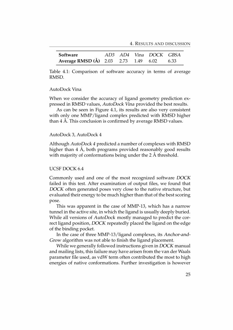
Software AD3 AD4 Vina DOCK GBSAAverage RMSD (Å) 2.03 2.73 1.49 6.02 6.33

Table 4.1: Comparison of software accuracy in terms of averageRMSD.

AutoDock Vina

When we consider the accuracy of ligand geometry prediction ex-pressed in RMSD values, AutoDock Vina provided the best results.

As can be seen in Figure 4.1, its results are also very consistentwith only one MMP/ligand complex predicted with RMSD higherthan 4 Å. This conclusion is confirmed by average RMSD values.

AutoDock 3, AutoDock 4

Although AutoDock 4 predicted a number of complexes with RMSDhigher than 4 Å, both programs provided reasonably good resultswith majority of conformations being under the 2 Å threshold.

UCSF DOCK 6.4

Commonly used and one of the most recognized software DOCKfailed in this test. After examination of output files, we found thatDOCK often generated poses very close to the native structure, butevaluated their energy to be much higher than that of the best scoringpose.

This was apparent in the case of MMP-13, which has a narrowtunnel in the active site, in which the ligand is usually deeply buried.While all versions of AutoDock mostly managed to predict the cor-rect ligand position, DOCK repeatedly placed the ligand on the edgeof the binding pocket.

In the case of three MMP-13/ligand complexes, its Anchor-and-Grow algorithm was not able to finish the ligand placement.

While we generally followed instructions given in DOCK manualand mailing lists, this failure may have arisen from the van der Waalsparameter file used, as vdW term often contributed the most to highenergies of native conformations. Further investigation is however

25


needed to confirm the cause.

4.1.2 Binding affinity prediction

Figure 4.2 show binding trends predicted by each docking software.Each data point represents one complex and the complexes are or-dered by decreasing binding potency (expressed in kcal/mol as neg-ative free energy of binding or negative binding score) as determinedfrom experimental data. For a list of MMP/ligand complexes or-dered by binding energy see Section 8.2.

To see how accurately docking software predicted binding trend,we calculated Spearman’s rank correlation coefficient and Pearson’ssample correlation coefficient. The values are shown in Table 4.2.

Initial values of Pearson’s coefficient (r1) were close to zero, sug-gesting weak predictive capability of tested software. As Pearson’scorrelation coefficient is much more sensitive to presence of outliers,we examined the data sets and identified several outliers.

Exclusion of three out of thirty-eight data points significantly in-creased Pearson’s sample correlation coefficient (r2), most notably incase of AutoDock 4.

Software AD3 AD4 Vina DOCK GBSAr1 0.06 0.05 -0.04 -0.01 -0.21r2 0.25 0.45 0.10 -0.01 -0.21ρs 0.001 0.23 -0.06 0.09 -0.13

Table 4.2: Pearson’s sample correlation coefficients including (r1) andexcluding (r2) outliers and Spearman’s rank correlation coefficients(ρs).

These results suggest that while docking programs are often ableto predict correct binding modes of MMP/ligand complexes, theyare still inaccurate in the field of binding affinity prediction. This is inagreement with recently published article [49], in which the authorstested several commercially available docking programs.

26


0,0

2,0

4,0

6,0

8,0

10,0

12,0

14,0

16,0

18,0

20,0

Bin

din

g sc

ore

MMP/ligand complex

AutoDock 3

1 5 10 15 20 25 30 35 1 5 10 15 20 25 30 35

Experiment

0,0

2,0

4,0

6,0

8,0

10,0

12,0

14,0

16,0

18,0

20,0

Bin

din

g sc

ore

MMP/ligand complex

AutoDock VinaAutoDock 4

1 5 10 15 20 25 30 35 1 5 10 15 20 25 30 35

0,0

0,0

10,0

20,0

30,0

40,0

50,0

60,0

70,0

80,0

90,0

Bin

din

g sc

ore

MMP/ligand complex

GBSA scoreDOCK score

1 5 10 15 20 25 30 35 1 5 10 15 20 25 30 35

Figure 4.2: Comparison of experimental binding energy and bindingscore predicted by each software.

27


4.2 Publication outputs

The results reported in this thesis have also been published at theconference:

Ryška J., Mishra S. K., Svobodová Vareková R., Koca J.: Dockingstudy of matrix metalloproteinase inhibitors. IX Discussions in Struc-tural Molecular Biology, 2011. (Poster, March 2011)

28

5 Conclusions

This thesis is focused on evaluation of molecular docking methodsand their applications in structure-based drug design.

The first part provides an introduction to the in silico moleculardocking techniques. It also presents information on the family of ma-trix metalloproteinases, zinc-dependent proteins used in this studyto compare accuracy of docking software.

The second part describes in detail the docking procedure, whichwas used in docking of MMP/ligand complexes, as well as overviewof the tested software and criteria used in their assessment.

The third part presents docking results obtained from individualprograms and their comparison. These results show that recently de-veloped AutoDock Vina finds the conformation of the ligands clos-est to the crystal structure. All tested programs had however signifi-cant problems with prediction of reasonable binding energies for thedocked complex.

Further work may include closer examination of UCSF DOCKresults and refinement of its docking procedure for metalloproteins.In future research, AutoDock Vina can be used for docking of thecompounds of our interest whose crystal structure is not known. Toget the accurate idea about the binders, binding energy calculationshould be performed using some molecular dynamics based free en-ergy calculation methods like LIE or MM-PBSA.

29

6 Summary

Molecular docking is an important tool in computational chemistryand computer-aided drug design. The goal of ligand-protein dockingis to identify favored binding modes of a ligand with a protein ofknown three-dimensional structure.

This thesis is focused on describing several approaches and al-gorithms used to find the optimal conformation of resulting ligand-protein complex. It also aims to provide overview and assessment ofseveral commonly used docking software.

We tested the programs on a set of matrix metalloproteinasesto evaluate their accuracy and treatment of metal atoms. The ini-tial protein and ligand structures have been optimized, docked witheach software and the results have been compared with experimentaldata.

While the software were often able to find correct ligand confor-mations, the results revealed significant problems of tested dockingsoftware in prediction of binding energy.

30

7 Souhrn

Molekulové dokování je duležitým nástrojem používaným v mnohaoblastech výpocetní chemie. Cílem protein-ligand dokování je naleze-ní energeticky výhodných vazebných módu ligandu s proteinem, je-hož trojrozmernou strukturu známe.

Tato práce je zamerena na popis nekolika bežných postupu a al-goritmu používaných pri hledání optimální konformace výslednéhoprotein-ligand komplexu. Klade si též za cíl poskytnout prehled asrovnání nekolika bežne používaných dokovacích programu.

Software byl testován na rodine matrix metalloproteinas za úcel-em ohodnocení, jak jednotlivé programy zacházejí s atomy kovu.Struktury všech proteinu i ligandu byly optimalizovány, dokoványvšemi programy a výsledky byly srovnány s experimentálne namere-nými daty.

Hodnocený software byl v mnoha prípadech schopen najít správ-nou konformaci ligandu, nicméne výsledky ukazují závažné prob-lémy pri výpoctu vazebných energií výsledných komplexu.

31

8 Appendices

8.1 Docking results by receptor

Following tables present values of RMSD and binding scores (ener-gies) predicted by AutoDock 3 (AD3), AutoDock 4 (AD4), AutoDockVina (Vina) and two methods (original DOCK score and GBSA re-scoring) implemented in UCSF DOCK 6.4.

MMP-1

RMSD (Å)PDB ID Ligand AD3 AD4 Vina DOCK GBSA966C RS2 0.86 0.98 1.13 2.64 3.593AYK CGS 2.05 1.94 1.87 4.46 7.541FBL HTA 3.72 6.21 1.83 7.32 7.352TCL RO4 2.38 2.00 2.40 7.50 7.481HFC PLH 2.81 6.31 2.13 6.49 6.66

Table 8.1: RMSD values of MMP-1/ligand complexes.

Binding score / energy (kcal/mol)PDB ID Exp. AD3 AD4 Vina DOCK GBSA966C -10.4 -12.0 -8.8 -9.7 -66.8 -14.43AYK -10.6 -10.4 -6.6 -7.3 -62.4 +0.21FBL -11.2 -9.5 -7.5 -6.9 -68.2 -20.52TCL -10.0 -9.2 -6.8 -6.7 -74.7 -41.71HFC -11.1 -11.3 -8.6 -7.6 -68.8 -29.0

Table 8.2: Binding score/energy values of MMP-1/ligand complexes.

32

8. APPENDICES

MMP-3

RMSD (Å)PDB ID Ligand AD3 AD4 Vina DOCK GBSA1G05 BBH 1.56 6.42 0.95 1.60 1.542JT5 JT5 1.63 1.25 1.77 8.83 3.072JT6 JT6 1.76 1.42 1.56 1.34 1.752JNP NGH 0.95 1.16 2.65 2.50 2.401G4K HQQ 1.24 1.65 1.04 2.80 3.041BIW S80 1.87 1.63 1.04 7.87 10.341B3D S27 2.14 2.14 1.39 7.82 7.591D5J MM3 0.56 0.61 1.12 1.77 2.241D7X SPC 0.80 0.71 0.72 0.90 1.341D8F SPI 2.72 2.61 1.94 8.79 8.591G49 111 1.36 1.68 1.57 4.24 1.352D1O FA4 2.15 3.67 2.65 13.22 13.09


Binding score / energy (kcal/mol)PDB ID Exp. AD3 AD4 Vina DOCK GBSA1G05 -11.6 -10.6 -8.9 -8.7 -68.7 -42.72JT5 -9.7 -11.2 -9.4 -9.4 -61.7 -21.72JT6 -9.5 -11.2 -9.7 -9.6 -63.6 -23.52JNP -9.8 -8.1 -6.7 -6.7 -65.1 -24.41G4K -8.3 -11.1 -9.3 -10.1 -54.2 -18.31BIW -9.5 -10.4 -8.2 -7.9 -24.3 -16.61B3D -10.4 -7.8 -7.8 -7.9 -52.6 -19.71D5J -12.5 -11.0 -9.8 -8.6 -55.7 -20.81D7X -10.5 -10.0 -8.2 -7.6 -70.6 -28.21D8F -10.6 -10.4 -9.5 -8.8 -48.1 -33.31G49 -10.6 -9.8 -8.0 -8.5 -78.1 -33.42D1O -10.5 -12.0 -5.0 -8.1 -36.8 -28.1


33

8. APPENDICES

MMP-7

RMSD (Å)PDB ID Ligand AD3 AD4 Vina DOCK GBSA1MMQ RRS 1.05 0.62 0.41 10.32 8.99


Binding score / energy (kcal/mol)PDB ID Exp. AD3 AD4 Vina DOCK GBSA1MMQ -11.6 -12.8 -10.1 -8.7 -39.3 -20.6


MMP-8

RMSD (Å)PDB ID Ligand AD3 AD4 Vina DOCK GBSA1ZP5 2NI 1.32 3.21 1.42 1.27 1.263DNG AXA 1.20 1.16 0.82 11.71 11.753DPE AXB 1.21 1.32 0.92 6.19 6.061ZVX FIN 1.72 1.15 1.67 6.32 6.871ZS0 EIN 1.71 1.90 1.34 6.44 6.331MNC PLH 2.02 6.08 1.54 6.44 6.42

Table 8.7: RMSD values of MMP-8/ligand complexes.Binding score / energy (kcal/mol)

PDB ID Exp. AD3 AD4 Vina DOCK GBSA1ZP5 -4.0 -11.7 -12.2 -10.4 -62.8 -41.73DNG -11.1 -15.5 -10.4 -12.4 -33.2 -22.83DPE -9.9 -17.5 -12.0 -12.8 -43.4 -9.81ZVX -12.6 -11.8 -10.3 -10.2 -63.1 -41.51ZS0 -8.4 -12.2 -10.8 -10.3 -66.1 -55.31MNC -11.9 -9.9 -9.7 -8.2 -71.5 -37.2


34

8. APPENDICES

MMP-9

RMSD (Å)PDB ID Ligand AD3 AD4 Vina DOCK GBSA2OVX 4MR 8.41 2.37 1.72 8.24 12.12


Binding score / energy (kcal/mol)PDB ID Exp. AD3 AD4 Vina DOCK GBSA2OVX -11.9 -12.9 -9.7 -11.3 -30.8 -15.7

Table 8.10: Binding score/energy values of MMP-9/ligand com-plexes.

MMP-12

RMSD (Å)PDB ID Ligand AD3 AD4 Vina DOCK GBSA1JIZ CGS 1.24 1.21 1.41 4.78 10.671RMZ NGH 1.34 1.49 1.29 1.06 0.751Y93 HAE 2.32 2.31 0.83 0.83 2.03


Binding score / energy (kcal/mol)PDB ID Exp. AD3 AD4 Vina DOCK GBSA1JIZ -11.9 -10.1 -8.1 -7.6 -30.4 -17.51RMZ -10.9 -9.2 -8.8 -7.5 -68.4 -38.31Y93 -2.9 -5.1 -5.3 -4.3 -36.9 -23.3


35

8. APPENDICES

MMP-13

RMSD (Å)PDB ID Ligand AD3 AD4 Vina DOCK GBSA1CXV CBP 0.89 0.70 1.14 6.87 17.72830C RS1 1.05 0.76 0.61 1.56 1.793I7I 518 2.10 1.19 2.63 N/A N/A1XUC PB3 4.74 12.15 0.67 11.50 0.421XUD PB4 N/A 3.12 0.61 11.96 16.761XUR PB5 3.59 8.53 0.98 10.90 13.602PJT 347 2.64 1.82 1.95 N/A N/A2D1N FA4 1.77 2.37 1.77 N/A N/A1YOU PFD 2.87 2.53 1.14 9.52 3.19


Binding score / energy (kcal/mol)PDB ID Exp. AD3 AD4 Vina DOCK GBSA1CXV -13.3 -12.6 -11.2 -9.9 -27.0 -16.3830C -12.9 -13.4 -12.4 -10.4 -82.1 -28.43I7I -8.5 -14.7 -13.7 -11.6 N/A -N/A1XUC -9.7 -12.7 -8.1 -11.5 -64.8 -46.91XUD -11.0 N/A -8.2 -11.9 -66.4 -28.71XUR -7.1 -12.5 -6.6 -10.5 -64.6 -24.92PJT -8.3 -11.7 -8.5 -9.3 N/A N/A2D1N -11.1 -11.0 -7.5 -7.9 N/A N/A1YOU -12.1 -11.2 -9.9 -9.1 -61.2 -11.4


36

8. APPENDICES

MMP-20

RMSD (Å)PDB ID Ligand AD3 AD4 Vina DOCK GBSA2JSD NGH 1.37 5.23 3.97 4.62 5.90


Binding score / energy (kcal/mol)PDB ID Exp. AD3 AD4 Vina DOCK GBSA2JSD -10.6 -9.7 -8.9 -7.1 -69.7 -34.7


37

8. APPENDICES

8.2 List of complexes ordered by binding affinity

Table 8.17 lists all MMP/ligand complexes used in the course of thisthesis ordered by decreasing binding affinity.

The ranks of complexes correspond to the ranking of complexesin Figure 4.2.

Rank PDB ID ∆Gexp. Rank PDB ID ∆Gexp.

1 1CXV -13.3 20 2JSD -10.62 830C -12.7 21 1D7X -10.53 1ZVX -12.6 22 2D1O -10.54 1YOU -12.6 23 966C -10.45 1D5J -12.5 24 2JT6 -10.46 1FBL -12.3 25 1B3D -10.47 1MNC -11.9 26 1MMQ -10.38 2OVX -11.9 27 2TCL -10.19 1JIZ -11.9 28 3DPE -9.910 1G05 -11.6 29 2JNP -9.811 1HFC -11.1 30 1XUC -9.712 3DNG -11.1 31 1BIW -9.513 2D1N -11.1 32 3I7I -8.514 1XUD -11.0 33 1ZS0 -8.415 1RMZ -10.9 34 2PJT -8.316 3AYK -10.6 35 1G4K -7.817 2JT5 -10.6 36 1XUR -7.118 1D8F -10.6 37 1Y93 -7.019 1G49 -10.6 38 1ZP5 -4.0

Table 8.17: MMP/ligand complexes ordered by binding affinity.

38

8. APPENDICES

8.3 Contents of the attached CD

• Receptor and ligand structures used in docking(folder TestSet).

• Table with complete results of docking simulations(folder Results).

• Text and source code of this thesis (folder Thesis).

39

Bibliography

[1] F. Jensen. Introduction to Computational Chemistry. John Wiley& Sons, 1999.

[2] T. Lengauer and M. Rarey. Computational methods forbiomolecular docking. Curr. Opin. Struct. Biol., 6(3):402–406,1996.

[3] D. B. Kitchen, H. Decornez, J. R. Furr, and J. Bajorath. Dockingand scoring in virtual screening for drug discovery: methodsand applications. Nature Reviews Drug Discovery, 3(11):935–949, 2004.

[4] D. A. Gschwend, A. C. Good, and I. D. Kuntz. Molecular dock-ing towards drug discovery. Journal of Molecular Recognition,9(2):175–186, 1996.

[5] J. J. Irwin, F. M. Raushel, and B. K. Shoichet. Virtual screeningagainst metalloenzymes for inhibitors and substrates. Biochem-istry, 44:12316–12328, 2005.

[6] R. P. Verma and C. Hansch. Matrix metalloproteinases (MMPs):Chemical-biological functions and (Q)SARs. Bioorg. Med.Chem., 15:2223–2268, 2007.

[7] F. X. Gomis-Ruth. Structural aspects of the metzincin clan ofmetalloendopeptidases. Mol. Biotechnol., 24(2):157–202, 2003.

[8] J. Gross and C. M. Lapiere. Collagenolytic activity in amphib-ian tissues: a tissue culture assay. Proc. Natl. Acad. Sci. USA,48(6):1014–1022, 1962.

[9] M. Egeblad and Z. Werb. New functions for the matrix met-alloproteinases in cancer progression. Nature Reviews Cancer,2:161–174, 2002.

[10] H. E. Van Vart and H. Birkedal-Hansen. The cysteine switch:a principle of regulation of metalloproteinase activity with po-tential applicability to the entire matrix metalloproteinase genefamily. Proc. Natl. Acad. Sci. USA, 87(14):5578–5582, 1990.

40

8. APPENDICES

[11] C. M. Overall and C. Lopez-Otin. Strategies for MMP inhibitionin cancer: innovations for the post-trial era. Nature ReviewsCancer, 2:657–672, 2002.

[12] M. D. Sternlicht and Z. Werb. How matrix metalloproteinasesregulate cell behavior. Annu. Rev. Cell. Dev. Biol., 17:463–516,2001.

[13] V. Aranapakam, J. M. Davis, G. T. Grosu, J. Baker, J. Elling-boe, A. Zask, J. I. Levin, V. P. Sandanayaka, M. Du, J. S. Skot-nicki, J. F. DiJoseph, A. Sung, M. A. Sharr, L. M. Killar, T. Walter,G. Jin, R. Cowling, J. Tillett, W. Zhao, J. McDevitt, and Z. B. Xu.Synthesis and structure-activity relationship of n-substituted 4-arylsulfonylpiperidine-4-hydroxamic acids as novel, orally ac-tive matrix metalloproteinase inhibitors for the treatment of os-teoarthritis. Journal of Medicinal Chemistry, 46(12):2376–2396,2003.

[14] M. Whittaker, C. D. Floyd, P. Brown, and A. J. Gearing. De-sign and therapeutic application of matrix metalloproteinase in-hibitors. Chem. Rev., 99:2735–2776, 1999.

[15] A. C. Wallace, R. A. Laskowski, and J. M. Thornton. LIGPLOT:a program to generate schematic diagrams of protein-ligand in-teractions. Protein Eng., 8:127–134, 1996.

[16] L. M. Coussens, B. Fingleton, and L. M. Matrisian. Matrixmetalloproteinases and cancer: Trials and tribulations. Science,295:2387–2392, 2002.

[17] F. Manello, G. Tonti, and S. Papa. Matrix metalloproteinase in-hibitors as anticancer therapeutics. Curr. Cancer Drug Targets,5:285–298, 2005.

[18] A. R. Leach. Molecular modelling: Principles and Applications,pages 662–663. Prentice Hall, second edition, 2001.

[19] C. A. Baxter, C. W. Murray D. E. Clark, D. R. Westhead, andM. D. Eldridge. Flexible docking using tabu search and an em-pirical estimate of binding affinity. Proteins: Structure, Function,and Bioinformatics, 33(3):367–382, 1998.

41

8. APPENDICES

[20] M. P. Allen and D. J. Tildesley. Computer Simulation of Liquids.Oxford University Press, 1989.

[21] B. Roux and T. Simonson. Implicit solvent models. Biophys.Chem., 78(1-2):1–20, 1999.

[22] I. Halperin, B. Ma, H. Wolfson, and R. Nussinov. Principles ofdocking: An overview of search algorithms and a guide to scor-ing functions. Proteins, 47(4):409–443, 2002.

[23] I. D. Kuntz, J. M. Blaney, S. J. Oatley, R. Langridge, and T. E.Ferrin. A geometric approach to macromolecule-ligand interac-tions. J. Mol. Biol., 161(2):269–288, 1982.

[24] D. P. Kroese, T. Taimre, and Z. I. Botev. Handbook of MonteCarlo Methods, page 772. John Wiley & Sons, 2011.

[25] C. M. Oshiro, I. D. Kuntz, and J. S. Dixon. Flexible liganddocking using a genetic algorithm. Journal of Computer-AidedMolecular Design, 9:113–130, 1995.

[26] P. J. Bowler. Evolution: The History of an Idea. University ofCalifornia Press, 2003.

[27] Ajay and M. A. Murcko. Computational methods to predictbinding free energy in ligand-receptor complexes. J. Med.Chem., 38:4953–4967, 1995.

[28] J. Bostrøm, P.-O. Norrby, and T. J. Liljefors. Conformational en-ergy penalties of protein-bound ligands. Journal of Computa-tionally Aided Molecular Design, 12:383–396, 1998.

[29] H. M. Berman, J. Westbrook, Z. Feng, G. Gilliland, T. N. Bhat,H. Weissig, I. N. Shindyalov, and P. E Bourne. The Protein DataBank. Nucleic Acids Research, 28:235–242, 2000.

[30] M. J. Frisch, G. W. Trucks, H. B. Schlegel, G. E. Scuseria, M. A.Robb, J. R. Cheeseman, J. A. Montgomery, Jr., T. Vreven, K. N.Kudin, J. C. Burant, J. M. Millam, S. S. Iyengar, J. Tomasi,V. Barone, B. Mennucci, M. Cossi, G. Scalmani, N. Rega,G. A. Petersson, H. Nakatsuji, M. Hada, M. Ehara, K. Toyota,

42

8. APPENDICES

R. Fukuda, J. Hasegawa, M. Ishida, T. Nakajima, Y. Honda,O. Kitao, H. Nakai, M. Klene, X. Li, J. E. Knox, H. P. Hratchian,J. B. Cross, V. Bakken, C. Adamo, J. Jaramillo, R. Gomperts, R. E.Stratmann, O. Yazyev, A. J. Austin, R. Cammi, C. Pomelli, J. W.Ochterski, P. Y. Ayala, K. Morokuma, G. A. Voth, P. Salvador, J. J.Dannenberg, V. G. Zakrzewski, S. Dapprich, A. D. Daniels, M. C.Strain, O. Farkas, D. K. Malick, A. D. Rabuck, K. Raghavachari,J. B. Foresman, J. V. Ortiz, Q. Cui, A. G. Baboul, S. Clifford,J. Cioslowski, B. B. Stefanov, G. Liu, A. Liashenko, P. Piskorz,I. Komaromi, R. L. Martin, D. J. Fox, T. Keith, M. A. Al-Laham,C. Y. Peng, A. Nanayakkara, M. Challacombe, P. M. W. Gill,B. Johnson, W. Chen, M. W. Wong, C. Gonzalez, and J. A. Pople.Gaussian 03, Revision E.01. Gaussian, Inc., Wallingford, CT,2004.

[31] J. Wang, W. Wang, P. A. Kollman, and D. A. Case. Automaticatom type and bond type perception in molecular mechanicalcalculations. Journal of Molecular Graphics and Modelling,25:247–260, 2006.

[32] University of California San Francisco. The Amber MolecularDynamics Package. http://ambermd.org/, 2011. [Online;accessed 22-April-2011].

[33] University of California San Francisco. UCSF Chimera HomePage. http://www.cgl.ucsf.edu/chimera/, 2011. [On-line; accessed 22-April-2011].

[34] R. Guha, M. T. Howard, G. R. Hutchison, P. Murray-Rust,H. Rzepa, C. Steinbeck, J. K. Wegner, and E. L. Willighagen. TheBlue Obelisk–Interoperability in Chemical Informatics. Journalof Chemical Information and Modeling, 46:991–998, 2006.

[35] G. M. Morris, R. Huey, W. Lindstrom, M. F. Sanner, R. K. Belew,D. S. Goodsell, and A. J. Olson. Automated docking using alamarckian genetic algorithm and and empirical binding freeenergy function. Journal of Computational Chemistry, 19:1639–1662, 1998.

43

http://ambermd.org/

http://www.cgl.ucsf.edu/chimera/

8. APPENDICES

[36] G. M. Morris, D. S. Goodsell, R. Huey, W. E. Hart, S. Halliday,R. Belew, and A. J. Olson. AutoDock 3 User’s Guide.

[37] M. Prokop et. al. TRITON: a graphical tool for ligand-bindingprotein engineering. Bioinformatics, 24:1955–1956, 2008.

[38] S. J. Weiner, P. A. Kollman, D. A. Case, U. C. Singh, C. Ghio,G. Alagona, S. Profeta, and P. Weiner. A new force field formolecular mechanical simulation of nucleic acids and proteins.Journal of the American Chemical Society, 106(3):765–784, 1984.

[39] X. Hu and W. H. Shelver. Docking studies of matrix metallopro-teinase inhibitors: zinc parameter optimization to improve thebinding free energy prediction. Journal of Molecular Graphicsand Modelling, 22(2):115–126, 2003.

[40] G. M. Morris, D. S. Goodsell, R. S. Halliday, R. Huey, W. E. Hart,R. K. Belew, and A. J. Olson. AutoDock4 and AutoDockTools4:Automated docking with selective receptor flexibility. Journalof Computational Chemistry, 30(16):2785–2791, 2009.

[41] O. Trott and A. J. Olson. Autodock Vina: improving the speedand accuracy of docking with a new scoring function, efficientoptimization, and multithreading. Journal of ComputationalChemistry, 31(2):455–461, 2010.

[42] M. F. Sanner. Python: A programming language for softwareintegration and development. Journal of Molecular Graphicsand Modelling, 17:57–61, 1999.

[43] D. Qui, P. Shenkin, F. Hollinger, and W. Still. The GB/SAcontinuum model for solvation. a fast analytical method forthe calculation of approximate born radii. J. Phys. Chem. A.,101(16):3005–3014, 1997.

[44] A. Jakalian, D. B. Jack, and C. I. Bayly. Fast, efficient generationof high-quality atomic charges. AM1-BCC model: II. Parameter-ization and validation. J Comput Chem, 23(16):1623–1641, 2002.

44

8. APPENDICES

[45] C. Huang. dms. http://www.cgl.ucsf.edu/chimera/docs/UsersGuide/midas/dms1.html, 2011. [Online; ac-cessed 22-April-2011].

[46] E. W. Weisstein. Root-mean-square. http://mathworld.wolfram.com/Root-Mean-Square.html, 2011. [Online; ac-cessed 22-April-2011].

[47] W. Humphrey, A. Dalke, and K. Schulten. VMD – Visual Molec-ular Dynamics. Journal of Molecular Graphics, 14:33–38, 1996.

[48] The Scripps Research Institute. AutoDock - AutoDock. http://autodock.scripps.edu/, 2011. [Online; accessed 22-April-2011].

[49] D. Plewczynski, M. Łazniewski, M. von Grotthuss, L. Rych-lewski, and K. Ginalski. Votedock: Consensus docking methodfor prediction of protein-ligand interactions. Journal of Compu-tational Chemistry, 32(4):568–581, 2011.

[50] J. L. Rodgers and W. A. Nicewander. Thirteen ways to look atthe correlation coefficient. The American Statistician, 42(1):59–66, 1988.

[51] J. L. Myers and A. D. Well. Research Design and Statistical Anal-ysis, page 508. Lawrence Erlbaum, 2003.

45

http://www.cgl.ucsf.edu/chimera/docs/UsersGuide/midas/dms1.html

http://www.cgl.ucsf.edu/chimera/docs/UsersGuide/midas/dms1.html

http://mathworld.wolfram.com/Root-Mean-Square.html

http://mathworld.wolfram.com/Root-Mean-Square.html

http://autodock.scripps.edu/

http://autodock.scripps.edu/

Docking study of matrix metalloproteinase inhibitors - Muni

Documents

Transcript of Docking study of matrix metalloproteinase inhibitors - Muni