
ANZSBT Guidelines Administration Blood Products 2ndEd Dec 2011 Hyperlinks
Upload
mick-geratowskiCategory
view
248download
4
International Civil Aviation Organization
Approved by the Secretary Generaland published under his authority
Manual on AutomaticMeteorologicalObserving Systemsat Aerodromes
Second Edition — 2011
Doc 9837AN/454


Doc 9837 AN/454
Manual on Automatic Meteorological Observing Systems at Aerodromes
________________________________
Approved by the Secretary Generaland published under his authority
Second Edition — 2011
International Civil Aviation Organization
Published in separate English, Arabic, Chinese, French, Russian and Spanish editions by the INTERNATIONAL CIVIL AVIATION ORGANIZATION 999 University Street, Montréal, Quebec, Canada H3C 5H7 For ordering information and for a complete listing of sales agents and booksellers, please go to the ICAO website at www.icao.int First edition 2006 Second edition 2011 Doc 9837, Manual on Automatic Meteorological Observing Systems at Aerodromes Order Number: 9837 ISBN 978-92-9231-799-7 © ICAO 2011 All rights reserved. No part of this publication may be reproduced, stored in a retrieval system or transmitted in any form or by any means, without prior permission in writing from the International Civil Aviation Organization.

(iii)
AMENDMENTS
Amendments are announced in the supplements to the Catalogue of ICAO Publications; the Catalogue and its supplements are available on the ICAO website at www.icao.int. The space below is provided to keep a record of such amendments.
RECORD OF AMENDMENTS AND CORRIGENDA
AMENDMENTS CORRIGENDA
No. Date Entered by No. Date Entered by


(v)
TABLE OF CONTENTS
Page Chapter 1 Introduction ................................................................................................................................. 1-1 Chapter 2. Explanation of terms .................................................................................................................. 2-1 Chapter 3. Wind ............................................................................................................................................ 3-1 3.1 Introduction ..................................................................................................................................... 3-1 3.2 Measurement methods ................................................................................................................... 3-1 3.3 Algorithms and reporting ................................................................................................................ 3-1 3.4 Sources of error and maintenance ................................................................................................. 3-5 3.5 Calibration and maintenance .......................................................................................................... 3-7 3.6 Measurement locations .................................................................................................................. 3-7 Chapter 4. Visibility ...................................................................................................................................... 4-1 4.1 Introduction ..................................................................................................................................... 4-1 4.2 Measurement methods ................................................................................................................... 4-2 4.3 Algorithms and reporting ................................................................................................................ 4-2 4.4 Sources of error .............................................................................................................................. 4-5 4.5 Calibration and maintenance .......................................................................................................... 4-5 4.6 Measurement locations .................................................................................................................. 4-6 Chapter 5. Runway visual range ................................................................................................................. 5-1 5.1 Introduction ..................................................................................................................................... 5-1 5.2 Reporting in METAR/SPECI ........................................................................................................... 5-1 Chapter 6. Present weather ......................................................................................................................... 6-1 6.1 Introduction ..................................................................................................................................... 6-1 6.2 Measurement methods ................................................................................................................... 6-1 6.3 Instrument limitations ...................................................................................................................... 6-4 6.4 Algorithms and reporting ................................................................................................................ 6-4 6.5 Sources of error .............................................................................................................................. 6-10 6.6 Calibration and maintenance .......................................................................................................... 6-11 6.7 Measurement locations .................................................................................................................. 6-11 Chapter 7. Clouds ......................................................................................................................................... 7-1 7.1 Introduction ..................................................................................................................................... 7-1 7.2 Measurement methods ................................................................................................................... 7-1 7.3 Algorithms and reporting ................................................................................................................ 7-3 7.4 Sources of error .............................................................................................................................. 7-4 7.5 Calibration and maintenance .......................................................................................................... 7-7 7.6 Measurement locations .................................................................................................................. 7-7

(vi) Manual on Automatic Meteorological Observing Systems at Aerodromes
Page
Chapter 8. Air temperature and dew-point temperature ........................................................................... 8-1 8.1 Introduction ..................................................................................................................................... 8-1 8.2 Measurement methods ................................................................................................................... 8-1 8.3 Sources of error .............................................................................................................................. 8-3 8.4 Measurement locations .................................................................................................................. 8-3 Chapter 9. Pressure ...................................................................................................................................... 9-1 9.1 Introduction ..................................................................................................................................... 9-1 9.2 Algorithms ...................................................................................................................................... 9-1 9.3 Sources of error .............................................................................................................................. 9-2 9.4 Calibration and maintenance .......................................................................................................... 9-3 9.5 Measurement locations .................................................................................................................. 9-3 Chapter 10. Supplementary information .................................................................................................... 10-1 Chapter 11. Integrated measurement systems .......................................................................................... 11-1 11.1 Categories of integrated measurement systems ............................................................................ 11-1 11.2 Calculation of meteorological parameters ...................................................................................... 11-3 11.3 Archiving of data ............................................................................................................................. 11-3 11.4 Data acquisition techniques ............................................................................................................ 11-5 11.5 Performance check and maintenance ............................................................................................ 11-5 11.6 Frequency of issue ......................................................................................................................... 11-5 Chapter 12. Remote sensing ....................................................................................................................... 12-1 12.1 Introduction ..................................................................................................................................... 12-1 12.2 Measurement methods and potentials............................................................................................ 12-1 Chapter 13. Quality assurance .................................................................................................................... 13-1 Appendix A. Algorithms ............................................................................................................................... App A-1 Appendix B. Specifying meteorological instruments for automatic meteorological observing systems ................................................................................................................ App B-1 Appendix C. Bibliography ............................................................................................................................ App C-1
___________________
1-1
Chapter 1
INTRODUCTION
1.1 The purpose of this manual is to help design or update automatic measurement systems for airports and understand the characteristics and limitations of such systems. The manual also deals with performance control and maintenance, as well as with maintaining the optimum operating conditions. 1.2 The chapters in this manual are organized according to parameter type and are presented in the same order as Annex 3 — Meteorological Service for International Air Navigation, Chapter 4 and Appendix 3. 1.3 The objective of this manual is not to describe all possible measurement methods; WMO’s Guide to Meteorological Instruments and Methods of Observation (WMO–No. 8), which is regularly reviewed and revised by WMO as necessary, describes these methods in detail. This manual takes this Guide into account but describes only those aspects which are useful or specific to the field of aeronautical meteorology. 1.4 The Manual of Runway Visual Range Observing and Reporting Practices (Doc 9328) describes all aspects related to runway visual range (RVR) and, to a large extent, visibility. This manual therefore does not go into detail about those elements. 1.5 The automatic observation of clouds and present weather is a new area of study and cannot yet meet all the needs expressed in Annex 3. The algorithms used are constantly evolving, making it difficult to standardize them at the present time. As a result, this manual indicates the basic principles only.
___________________


2-1
Chapter 2
EXPLANATION OF TERMS
Note.— These explanations are generally based on established scientific definitions, some of which have been simplified to assist non-specialist readers. Approved ICAO definitions are marked with an asterisk (*) and published WMO definitions1 with a double asterisk (**). The units, where appropriate, are indicated in brackets. Air temperature. The temperature indicated by a thermometer exposed to the air in a place sheltered from direct solar
radiation (degree Celsius, °C). Allard’s law. An equation relating illuminance (E) produced by a point source of light of intensity (I) on a plane normal to
the line of sight, at distance (x) from the source, in an atmosphere having a transmissivity (T). Note.— Applicable to the visual range of lights. Atmospheric pressure. Pressure (force per unit area) exerted by the atmosphere on any surface by virtue of its weight; it
is equivalent to the weight of a vertical column of air extending above a surface of unit area to the outer limit of the atmosphere (hectopascal, hPa).
Ceilometer. Instrument for measuring the height of the base of a cloud layer, with or without a recording device.
Measurement done by calculating the return time of laser light pulses reflected by the cloud base. Cloud amount. The fraction of the sky covered by the clouds of a certain genus, species, variety, layer, or combination of
clouds. Cloud base. The lowest level of a cloud or cloud layer (metre, m, or foot, ft). Convective cloud. Cumuliform clouds which form in an atmospheric layer made unstable by heating at the base or
cooling at the top. Dedicated display. A display connected to a sensor, designed to provide a direct visualization of the operational
variables. Dew-point temperature. Temperature to which a volume of air must be cooled at constant pressure and constant
moisture in order to reach saturation; any further cooling causes condensation (degree Celsius, °C). Disdrometer. A device used for catching the drops of liquid hydrometeors and for measuring the distribution of their
diameters.
1. Guide to Meteorological Instruments and Methods of Observation (WMO – No. 8).

2-2 Manual on Automatic Meteorological Observing Systems at Aerodromes
Extinction coefficient (σ).** The proportion of luminous flux lost by a collimated beam, emitted by an incandescent source at a colour temperature of 2 700 K, while travelling the length of a unit distance in the atmosphere (per metre, m–1).
Note.— The coefficient is a measure of the attenuation due to both absorption and scattering. Illuminance (E).** The luminous flux per unit area (lux, lx). Koschmieder’s law. A relationship between the apparent luminance contrast (Cx) of an object, seen against the horizon
sky by a distant observer, and its inherent luminance contrast (C0), i.e. the luminance contrast that the object would have against the horizon when seen from very short range.
Note. — Applicable to the visual range of objects by day. Lightning detection network. Network of lightning detectors transmitting in real time to a central computer, locating
lightning flashes by combining information received from each detector. Luminance (photometric brightness) (L). The luminous intensity of any surface in a given direction per unit of projected
area (candela per square metre, cd/m2). Luminance contrast (C). The ratio of the difference between the luminance of an object and its background to the
luminance of the background (dimensionless). Luminous intensity (I).** The luminous flux per unit solid angle (candela, cd). Magnetic wind direction. The direction, with respect to magnetic north, from which the wind is blowing. The magnetic
wind directions are used in aircraft operations, necessitated by the magnetic frame of reference applied to air navigation facilities (degree).
Meteorological optical range (MOR).** The length of the path in the atmosphere required to reduce the luminous flux in
a collimated beam from an incandescent lamp, at a colour temperature of 2 700 K, to 0.05 of its original value, the luminous flux being evaluated by means of the photometric luminosity function of the International Commission on Illumination (CIE) (metre, m, or kilometre, km).
Note.— The relationship between meteorological optical range and extinction coefficient (at the contrast threshold of ε = 0.05) using Koschmieder’s law is: MOR = −In(0.05)/σ ≈ 3/σ. MOR = visibility under certain conditions (see Visibility). Precipitation intensity. An indication of the amount of precipitation collected per unit time interval. It is expressed as light,
moderate or heavy. Each intensity is defined with respect to the type of precipitation occurring, based on rate of fall. Present weather. Weather existing at a station at the time of observation. Present weather sensor. Sensor measuring physical parameters of the atmosphere and calculating a limited set of
present weather, always including present weather related to precipitation. Prevailing visibility.* The greatest visibility value, observed in accordance with the definition of “visibility”, which is
reached within at least half the horizon circle or within at least half of the surface of the aerodrome. These areas could comprise contiguous or non-contiguous sectors (metre, m, or kilometre, km).
Note.— This value may be assessed by human observation and/or instrumented systems. When instruments are installed, they are used to obtain the best estimate of the prevailing visibility. QFE. Atmospheric pressure at aerodrome elevation (or at runway threshold) (hectopascal, hPa).
Chapter 2. Explanation of terms 2-3
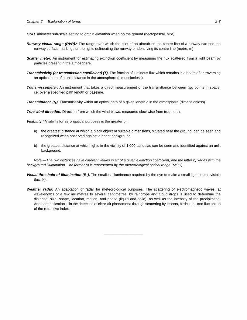
QNH. Altimeter sub-scale setting to obtain elevation when on the ground (hectopascal, hPa). Runway visual range (RVR).* The range over which the pilot of an aircraft on the centre line of a runway can see the
runway surface markings or the lights delineating the runway or identifying its centre line (metre, m). Scatter meter. An instrument for estimating extinction coefficient by measuring the flux scattered from a light beam by
particles present in the atmosphere. Transmissivity (or transmission coefficient) (T). The fraction of luminous flux which remains in a beam after traversing
an optical path of a unit distance in the atmosphere (dimensionless). Transmissometer. An instrument that takes a direct measurement of the transmittance between two points in space,
i.e. over a specified path length or baseline. Transmittance (tb). Transmissivity within an optical path of a given length b in the atmosphere (dimensionless). True wind direction. Direction from which the wind blows, measured clockwise from true north. Visibility.* Visibility for aeronautical purposes is the greater of: a) the greatest distance at which a black object of suitable dimensions, situated near the ground, can be seen and
recognized when observed against a bright background; b) the greatest distance at which lights in the vicinity of 1 000 candelas can be seen and identified against an unlit
background. Note.—The two distances have different values in air of a given extinction coefficient, and the latter b) varies with the background illumination. The former a) is represented by the meteorological optical range (MOR). Visual threshold of illumination (ET). The smallest illuminance required by the eye to make a small light source visible
(lux, lx). Weather radar. An adaptation of radar for meteorological purposes. The scattering of electromagnetic waves, at
wavelengths of a few millimetres to several centimetres, by raindrops and cloud drops is used to determine the distance, size, shape, location, motion, and phase (liquid and solid), as well as the intensity of the precipitation. Another application is in the detection of clear-air phenomena through scattering by insects, birds, etc., and fluctuation of the refractive index.
___________________

3-1
Chapter 3
WIND
3.1 INTRODUCTION 3.1.1 Wind has a direct impact on aircraft. The direction of the prevailing wind is taken into account when planning a new runway. Headwind components determine the direction of take-off and landing and crosswinds force the pilot to compensate for the drift. 3.1.2 An important characteristic of wind is its temporal and spatial variability. Pilots need to be aware of local wind conditions at the airport, especially during approach and departure. Temporal variability makes it necessary to define multiple parameters related to wind: mean, minimum and maximum values. Spatial variability is mostly related to temporal variability and can, for example, lead to a relative movement of gusts (like ripples on a body of water). It can also be related to terrain effects of the aerodrome or its surroundings, or to the presence of obstacles. For these reasons, Annex 3 — Meteorological Service for International Air Navigation recommends that wind observations for local reports be representative of the touchdown zone (for arriving aircraft) and of conditions along the runway (for departing aircraft), which sometimes leads to the installation of multiple sensors.
3.2 MEASUREMENT METHODS 3.2.1 Wind measurements in support of aerodrome operations are carried out using anemometers. The most common of the rotating anemometers are cup or propeller anemometers, whose rotating speed is synchronous with wind speed; they are associated with wind vanes. The characteristics of such instruments are well defined in the Guide to Meteorological Instruments and Methods of Observation (WMO–No. 8). For these instruments, the time constant is equal to the distance constant, a characteristic of the anemometer, divided by the wind speed. For a classic distance constant of 5 m, the time constant for a speed of 10 m/s (20 kt) is 0.25 seconds. Extreme wind speed values calculated over 3 seconds, as recommended by Annex 3 and the WMO–No. 8, can therefore be easily measured with a cup or propeller anemometer. 3.2.2 There are also static hot-film sensors and ultrasonic sensors. The availability of ultrasonic anemometers on the market is, however, increasing because they do not have moving mechanical parts but are more technically complex and they can de-ice themselves better than most rotating sensors. Ultrasonic sensors also have a short time constant and are able to provide many measurement samples per second. It is, however, important to integrate these measurements over a 3-second period for speed and direction extremes to keep these extreme values from depending on the sampling rate of measurements.
3.3 ALGORITHMS AND REPORTING
3.3.1 Mean speed values 3.3.1.1 There are several methods of calculating mean wind speed. At each instant, a wind vector is available and characterized by its speed and direction.

3-2 Manual on Automatic Meteorological Observing Systems at Aerodromes
3.3.1.2 It is possible to calculate the mean wind vector over a given period by calculating the mean of the north/south and east/west components of each instantaneous wind vector, and by extracting the speed and direction of this mean wind vector. This type of calculation might seem logical given the nature of the information (a vector), but it does have some disadvantages: a) It depends on the actual availability of direction. If a wind vane breaks down when using an anemometer,
the “wind speed” parameter is no longer available; b) Mathematically, it can lead to a zero mean wind vector, although there are non-zero instantaneous wind
vectors, as a result of a wind change. This case is however theoretical, especially since such a change in wind can result in a marked discontinuity if the wind speed is high enough. Nevertheless, a reduction in the mean wind vector is possible if there is a change in direction with light winds; and
c) This is not the same method of calculation used in the past when electronic equipment for calculating
vectors did not exist. A temporal integration was done on the modulus of instantaneous wind with recorders.
3.3.1.3 It is also possible to calculate separately the mean wind speed using only the instantaneous speed by calculating the mean modulus of instantaneous wind vectors. This method has several advantages: a) It does not require the direction, and a breakdown of the wind vane does not result in the absence of
calculated speed parameters if there is a requirement to report wind speed without a direction and vice versa;
b) It is easier to implement; and c) It is closer to calculation techniques used in the past. Its disadvantage is that it gives a mean wind vector that is different from the vector mean of instantaneous winds. 3.3.1.4 ICAO and WMO have not yet provided recommendations on the calculation method, probably since both practices are used throughout the world and a vector calculation would cause problems in several areas. With modern systems, vector calculations are not a problem, especially since they are required for the mean direction. Differences in results between both calculations are minimal when there are few changes in wind direction but are greater when the wind direction shows great variability. If the speed is over 5 m/s (10 kt), there is marked discontinuity. If the speed is less than 5 m/s (10 kt), the differences (in absolute values) between both methods remain minimal.
3.3.2 Mean direction values 3.3.2.1 Similarly, the calculation can be vector or scalar (direct mean of directions), but the scalar mean of directions poses a major disadvantage in relation to the discontinuity of directions between 350° and 10°. The mean of directions varying between 350° and 10°, however, must not be 180°. It is possible to avoid this problem by introducing a drift in the directions, for example by considering a direction of 370° rather than 10°, but applying such a drift that depends on effectively measured directions can be difficult and can cause errors under certain conditions. 3.3.2.2 An example of an algorithm regarding wind direction (1) is given in Appendix A. 3.3.2.3 As a general rule, it is recommended that a vector calculation be performed, using either of these two methods: a) by calculating the mean wind vector and its direction; or

Chapter 3. Wind 3-3
b) by calculating the mean wind vector using the instantaneous vectors of a unit modulus and the direction equal to the measured direction. This method of calculation is somewhat simpler than calculating the actual mean wind vector. Unless there are significant variations in wind speed, it gives equivalent results, while significant variations in wind speed produce marked discontinuity.
3.3.3 Calculating a mean value Whether the calculation is vector or scalar, the term “mean” should be understood as an arithmetic mean over the given time period.
3.3.4 Calculating extreme values 3.3.4.1 Annex 3 requires that extreme speed and direction values be calculated over a 3-second period. These values should be calculated using measurement samples available every 250 ms (millisecond); however, it is recommended that these values be calculated using measurement samples available at least every second. The calculation should be made as the primary samples become available (e.g. every 250 ms, or at least every second); it should not be made every 3 seconds over a 3-second period, since the calculation would then depend on the calculation time window for wind speed fluctuations, which can be faster than this 3-second period. 3.3.4.2 It is also important for the instantaneous measurement used to be representative of the entire period separating two measurements. If this period is 500 ms, the measurement should be representative of the wind during these 500 ms. This is usually the case with rotating anemometers, whose measurement system counts the number of turns in a given period, which may not be the case for sensors with a faster pace of measurement.
3.3.5 Calculating mean values over 2 and 10 minutes For local reports, the calculation period is 2 minutes. For METAR/SPECI, the calculation period is usually 10 minutes, but it can be less in cases of marked discontinuity.
3.3.6 Marked discontinuity algorithm 3.3.6.1 Annex 3 defines a marked discontinuity as follows: “A marked discontinuity occurs when there is an abrupt and sustained change in wind direction of 30° or more, with a wind speed of 5 m/s (10 kt) before or after the change, or a change in wind speed of 5 m/s (10 kt) or more, lasting at least 2 minutes.” 3.3.6.2 Examples of algorithms on marked wind discontinuity (2 and 3) are given in Appendix A. 3.3.6.3 When a marked discontinuity is detected, the representative mean wind period (first 2 minutes, increased progressively to 10 minutes) must also be used to find the extreme speed and direction values.
3.3.7 Minimum and maximum speeds 3.3.7.1 Extreme wind speed values must be calculated using values that represent a 3-second period, over an adapted period (usually 10 minutes, but also between 2 and 10 minutes after a marked discontinuity). Extreme values can be calculated over successive 1-minute periods, then combined over the appropriate time period. 3.3.7.2 Maximum speed is included in both local reports and METAR/SPECI if the difference between the maximum and mean speed over 10 minutes (or a lesser time period after a marked discontinuity) is above or equal to 5 m/s (10 kt), in
3-4 Manual on Automatic Meteorological Observing Systems at Aerodromes
which case the minimum speed is then also included in local reports. It should be noted that a difference of 2.5 m/s (5 kt) between the maximum speed and the mean speed should be used when noise abatement procedures are applied in accordance with the Procedures for Air Navigation Services — Air Traffic Management (PANS-ATM, Doc 4444), 7.2.3. 3.3.7.3 Artificial gusts caused by jet efflux or wake vortices from aircraft may on occasion affect wind measurements. Measuring these artificial gusts should be avoided to the extent possible by appropriately siting the sensors (see discussion on the siting of sensors in 3.4.2). However, perfect siting of sensors may not be possible at many aerodromes. In the event that such artificial gusts cannot be avoided, they may be detected and, if necessary, removed in real time by an automated algorithm as a last resort. An example of such an algorithm on the detection and removal of artificial gusts (4) is given in Appendix A.
3.3.8 Extreme wind directions
3.3.8.1 The sector of variability in 3-second mean directions is limited by the two extreme direction values calculated in the preceding 10 minutes (time increment) and can be defined every minute using 3-second mean directions calculated as the data are received. These directions are placed in a direction histogram with a resolution of 10°. 3.3.8.2 The sector can be found in two steps using the direction of the mean wind in the given 10 minutes. Step one looks for the first limit by scanning the histogram directions counter-clockwise. Step two looks for the second limit by scanning the histogram directions clockwise. In both steps, the desired limit is the direction of the histogram adjacent to a sector with two consecutive directions of zero value. If the occurrence of the condition that determines one or more limits is not met (sector of 360°), the sector is declared undetermined. 3.3.8.3 This search is usually performed over a 10-minute period. After a marked discontinuity, however, the search period is lowered to 2 minutes and then increased progressively to 10 minutes. The wind direction is to be reported as variable if the wind direction varies in accordance with the criteria established in Annex 3.
3.3.9 Reporting wind direction
in local reports and METAR/SPECI Wind directions coded in METAR/SPECI and in local reports are given as the true wind direction, i.e. in relation to True North. However, wind direction provided to pilots, such as via automatic terminal information service (ATIS), is reported as the magnetic wind direction. The difference between reporting true and magnetic wind direction depends upon the aerodrome location in relation to the magnetic North Pole. The difference is sometimes small compared to the 10° coding resolution, but it can reach up to 20° or 30° in higher latitude regions of the world, rising to as much as 180° at the magnetic poles. Any ambiguity about the significance of directions must therefore be avoided between the service providing the observations and the aeronautical user. It is especially important for the controller to avoid performing a mental conversion using a value displayed in relation to True North. Controllers, in providing wind direction to the pilot, are required to report the magnetic wind direction; therefore, the wind displays at the air traffic services (ATS) units should automatically make the conversion from true to magnetic wind directions.
3.3.10 Changes in parameters
3.3.10.1 Wind is a parameter that is very variable in time (gusts) and space. As a result, there are different exposure requirements for sensors used in METAR/SPECI and those used in local reports. Sensors for surface wind observations for METAR/SPECI should be sited to give representative indications of conditions along the whole runway (at aerodromes with one runway) or the runway complex (where there is more than one runway). However, sensors for local reports (provided to aircraft taking-off and landing) are to be sited to give the best practicable indication of conditions along the
Chapter 3. Wind 3-5
runway (e.g. lift-off and touchdown zones). At aerodromes where topography or prevalent weather conditions cause significant differences in the surface wind at various sections of the runway, additional sensors should be installed. Sensors should not be sited close to obstacles that can affect measurements. Obstacles increase turbulence and can make wind direction more variable, leading to unnecessary reporting of wind variations, due to the change criterion of 60° in direction being exceeded artificially as a result of sensors being located close to obstacles. 3.3.10.2 When there are gusts, wind speed can suddenly increase or decrease, which explains the importance of observing both the maximum and minimum speed values. How much the speed changes depends on weather conditions and on the roughness of the surrounding land; rough land produces greater changes. On average, the ratio of maximum wind to mean wind over 10 minutes is close to 1.5, and the ratio of minimum wind to mean wind is close to 0.7. 3.3.10.3 High wind speed variability could make it tempting to use instantaneous wind, giving the impression that reality is being represented more accurately; this is a false impression and instantaneous wind should not be used (Annex 11, 4.3.6.1).
3.3.11 Wind reporting at the touchdown zone (TDZ) with multiple anemometers 3.3.11.1 Sensors for surface wind observations for local routine and special reports should be sited to give the best practicable indication of conditions along the runway and TDZ. Additional sensors should be provided at aerodromes where topography or prevalent weather conditions cause significant differences in surface wind at various sections of the runway. 3.3.11.2 With the presence of more than one anemometer within the same TDZ, there arises an issue concerning how to use the data from the various anemometers (based on an averaging period of two minutes) in the reporting of wind for the TDZ when the wind observations from these anemometers are significantly different, varying by, for example, more than ten per cent from each other. Based on discussions with the aviation users concerned, the following example to report the wind for a TDZ based on multiple anemometers was formulated taking into consideration the flight safety and users’ perspectives:
“when data from more than one anemometer are available at the same TDZ, only a single set of mean wind speed, mean wind direction and gust is to be reported to the users based on the readings from the multiple anemometers. The single set is taken as the maximum of the mean wind speeds from the anemometers, the corresponding mean wind direction of the anemometer recording the maximum mean wind speed, and the maximum of the gusts from the anemometers.”
3.3.11.3 It is noted that, given the proposed approach above, the anemometer used for reporting the mean wind speed and direction and the one used for reporting the gust for the TDZ concerned could be different. This is because the anemometer further away from buildings may record a higher value of the mean wind speed owing to a reduced shelter, but the anemometer closer to buildings may record a higher gust owing to the proximity to the turbulence flow associated with the buildings.
3.4 SOURCES OF ERROR AND MAINTENANCE
3.4.1 Sensors 3.4.1.1 Bearings on mechanical sensors can wear down, increasing the starting threshold. Such an increase can cause problems during light winds, but light wind speeds do not affect operations. For greater wind speeds, an increase in the starting threshold does not cause problems, since the torque exerted by the wind on cups or a propeller is proportional to the squared speed, so it quickly and greatly exceeds the resistance corresponding to the starting threshold: if the
3-6 Manual on Automatic Meteorological Observing Systems at Aerodromes
threshold is 2 m/s (4 kt), for a speed of 10 m/s (20 kt), the torque will be 25 times stronger. Nevertheless, wear can eventually lead to a blocking of the anemometer or wind vane. 3.4.1.2 One way to monitor the condition of bearings is to check the starting threshold. This can be done in a laboratory, making it necessary to change the on-site sensor. A simple technique can be used to monitor bearings: sheltered from the wind (in a vehicle or building), a pulse is given to the anemometer and the amount of time the rotation stops is measured. If the bearings are worn down, they will stop rotating for a shorter time than those of a sensor in good condition. The minimum amount of time required for the bearings to be considered in good condition depends on the type of anemometer. This method is simple and dependable and can also be used for a wind vane, by replacing the flat surface with cups (to limit aerodynamic braking and increase the inertia of the axis of rotation). 3.4.1.3 Another significant source of error with mechanical sensors is the accumulation of freezing or frozen precipitation on the moving parts. If wet snow clings to the surface of the rotating cups, a marked reduction in wind speed will be reported. Such conditions may also induce wind direction errors by greatly increasing the mass of the vane, reducing its sensitivity to changes. Similarly, freezing precipitation may disable both the wind speed and wind direction by immobilizing the moving parts. Some methods that have been employed to offset this include heating of various components of the instrument and the suppression or flagging of data when errors are likely or suspected. 3.4.1.4 Static sensors can be monitored in a zero wind chamber (in which the sensors are sometimes packaged), available through the sensor manufacturers’ catalogues.
3.4.2 Siting of sensors 3.4.2.1 Anemometers should be sited to provide representative wind measurements at an aerodrome. Guidance on siting of anemometers can be found in: a) Manual of Aeronautical Meteorological Practice (Doc 8896), Appendix 2; b) Guide to Meteorological Instruments and Methods of Observation (WMO-No. 8), Part I, Chapter 5; and c) Guide on Meteorological Observing and Information Distribution Systems for Aviation Weather Services
(WMO-No. 731), Chapter 2. 3.4.2.2 In siting an anemometer within an aerodrome, consideration of obstacle clearance rules should be taken into account (see 3.6). 3.4.2.3 The ICAO recommendation for the measurement of height (approximately 10 m) is a compromise between being high enough to avoid surface effects (such as friction) and an installation height that is practical and safe in the aerodrome environment. It is very important to install a sensor in the clearest location possible. As a minimum, it is recommended that any wind-measuring instrument be installed at a distance equal to at least 10 times the height of surrounding obstacles. 3.4.2.4 Sensors must never be installed on the roof of a building, such as a control tower, because the building itself affects the wind flow, which is accelerated at roof level or at the top of the building. For a sensor installed 2 or 3 m above a control tower, speed can by overestimated by 30 per cent. The overestimate will depend on the wind direction and the relative position of the sensor in relation to the edge and shape of the roof. 3.4.2.5 Whilst wind sensors should be located close to the runway(s) to achieve representative wind measurement, every effort should be made to site the sensors to minimize the effect from artificial gusts, e.g. due to jet efflux or wake vortices (see 3.3.7.3).

Chapter 3. Wind 3-7
3.4.3 Orientation of the sensor 3.4.3.1 A wind measurement sensor must be oriented to True North to indicate the direction correctly. The sensor’s design plays a part in determining how easily it can be oriented north. The stability of the fastener must also be checked to keep the sensor from rotating over time. 3.4.3.2 For the sensors to be accessible, the fastening mast can often be folded. The mast should have a mark, which must be positioned correctly towards the north. This can be checked with a magnetic compass aligned with the marker and installed in the same place as the sensor or wind vane. Without proper precautions, it is quite possible for alignment errors to exceed 10°.
3.5 CALIBRATION AND MAINTENANCE 3.5.1 For rotating anemometers, the response characteristics are essentially related to the characteristics of the cups or the propeller and wind vane flag. The bearings must be monitored regularly and changed, if necessary. With bearings in good condition, visually monitoring the condition of the cups or the propeller can be enough for the anemometer. An inexpensive way of making sure that these cups or propellers are in good condition is to make a preventative replacement of these elements at regular intervals (e.g. every 2 years). 3.5.2 It is also possible to use a motor whose rotation speed is known in order to train the axis of a rotating anemometer, which makes it possible to control the sensor’s transducer. 3.5.3 For static anemometers, a checkpoint is the zero wind chamber test. The stability of the characteristics of measurement ranges depends on the sensor’s design. Verifying the sensor’s response to the measurement ranges requires a wind tunnel test. For sonic anemometers, the standard used is International Organization for Standardization (ISO) standard 16622. 3.5.4 The orientation of the wind vane must be monitored regularly. If the mast bears a mark for orientation and its design makes it possible to guarantee the stability of its orientation, a simple visual check can suffice. This of course requires the sensor to be designed in such a way as to guarantee that the direction indication is aligned with the mark on the sensor: the quality and stability of the orientation depend largely on the sensor’s design.
3.6 MEASUREMENT LOCATIONS 3.6.1 Measurements cannot of course be taken on the runway, and it is important to follow the obstacle clearance rules in Annex 14 — Aerodromes, Volume I, Chapter 8, and the Airport Services Manual (Doc 9137), Part 6. The minimum distance of a 10-m frangible mast in relation to the runway centre line is 90 m. The mast must be placed in this zone only if absolutely necessary; in most circumstances, a 10-m mast should be at least 220 m from the runway centre line. These criteria are shown in more detail in Figure 3-1. 3.6.2 Multiple wind sensors are recommended for aerodromes subject to changing weather conditions as a result of terrain effects, land or sea breezes, widely spaced aerodromes, etc. Wind measurements for each runway also give a more comprehensive picture of runway conditions for take-off and landing and also provide back-up in case of sensor malfunction. 3.6.3 In METAR/SPECI, the wind measurement must be representative of the runway or runway complex. If only one wind measurement is taken at the airport, this measurement is used both for local reports and METAR/SPECI.

3-8 Manual on Automatic Meteorological Observing Systems at Aerodromes
3.6.4 With multiple sensors, one particular sensor deemed the most representative of the runway or runway complex is to be used for METAR/SPECI. In practice, such a sensor position is selected when the measurement system is being designed. Measurements that are too specific for a runway threshold and that would therefore be intended especially for this threshold, because of specific local conditions and not representative of the vicinity of the aerodrome, should not be selected. 3.6.5 With multiple sensors, it may be useful for the observation system to be able to accept a measurement from another suitable anemometer in case the sensor used for METAR/SPECI breaks down.

Chapter 3. Wind 3-9
Figure 3-1. Obstacle limitation surfaces
___________________
“OBSTACLE FREE ZONE” — Generally speaking no MET sensors should infringe this region unless exceptional local circumstances so dictate. In the latter case sensor supports must be frangible, lighted and if possible sensor should be “shielded” by an existing obstacle.
1) Transmissometer sited between 66 m and 120 m from runway centre line 2) Ceilometer may be sited in this region if not located near middle marker 3) If essential to locate within strip, anemometer height 10 m minimum distance from centre line = 90 m.
Usual location of anemometer masts minimum distance from runway centre line for 6 m mast is = 192 m and for a 10 m mast = 220 m, assuming surface wind observations made in this region are representative of conditions over runway.

4-1
Chapter 4
VISIBILITY
4.1 INTRODUCTION 4.1.1 Visibility is a crucial parameter for aeronautical operations. Low visibility below the approved minimum aircraft and flight crew certification can prevent aircraft from utilizing a runway. Visual aids (markings) and landing and take-off instruments are specifically set up to limit these operational restrictions. 4.1.2 The definition of visibility for aeronautical purposes is:
“Visibility for aeronautical purposes is the greater of: a) the greatest distance at which a black object of suitable dimensions, situated near the ground, can
be seen and recognized when observed against a bright background; b) the greatest distance at which lights in the vicinity of 1 000 candelas can be seen and identified
against an unlit background. Note.—The two distances have different values in air of a given extinction coefficient, and the latter
b) varies with the background illumination. The former a) is represented by the meteorological optical range (MOR).”
4.1.3 Visibility in a METAR/SPECI must be representative of the aerodrome, which is a wide area over which significant changes in visibility can take place, so it was necessary to find a synthetic way of describing these changes. Amendment 73 to Annex 3 introduced “prevailing visibility” (Chapter 2 refers). 4.1.4 The Manual of Runway Visual Range Observing and Reporting Practices (Doc 9328) describes the atmospheric phenomena that reduce visibility, the different measurement instruments and algorithms; these will not be covered in detail here. 4.1.5 The distinctive characteristics of automatic visibility observations are linked to the possible spatial changes in visibility. 4.1.6 For aeronautical purposes, the measurement range for visibility is from 25 m to 10 km. Values greater than or equal to 10 km are indicated as 10 km. A sensor must therefore be able to measure values above 10 km or indicate if the measurement is greater than or equal to 10 km. 4.1.7 The lower limit is actually linked to the resolution of 50 m required in reports. Measurement instruments often have a resolution smaller than 50 m in low values. Annex 3 specifies that visibility values should be rounded down to the nearest reporting step which means that a visibility value of 45 m will be reported as 0 m. Thus, any measurement of visibility below 50 m should be encoded as 0 m, whilst any visibility measurement between 50 m and 100 m should be encoded as 50 m.

4-2 Manual on Automatic Meteorological Observing Systems at Aerodromes
4.2 MEASUREMENT METHODS 4.2.1 Forward-scatter meters are suitable for evaluating the visibility measurement range. 4.2.2 Backward-scatter meters, which are generally more sensitive to the types of scattering particles (fog, dust, sand, rain and snow), should be avoided, except when they are able to identify these particles and take them into account. 4.2.3 A transmissometer has a measurement range linked to its base (distance between the transmitter and receiver). This base is adapted to the RVR range (50 to 1 500 or 2 000 m), which is too short to measure visibilities up to 10 km. However, there are double-base transmissometers that make it possible to cover a greater range of measurement. 4.2.4 There are also prototype systems that use a camera and automatically analyse an image by recognizing (or not recognizing) predefined marks. The advantage of this technique is that it could resemble a human observation and possibly provide an overview, but it would have the disadvantage of referring to a reference point. Continuous functioning in widespread luminance ranges is a difficult matter when trying to avoid sun glare. At night, only the luminous marks can be used, so they must exist. At present, no such validated systems are used. 4.2.5 Not all sensors available on the market perform equally accurately; in fact, there may be significant differences in performance, especially during precipitation. Doc 9328, Chapter 9, describes one method used to test visibility measurement sensors. 4.2.6 Calculating aeronautical visibility also requires the background luminance, measured by a background luminance sensor. Doc 9328, 9.1.5, describes the sensor needed to calculate the RVR. If it exists, it is possible to use the same sensor to calculate visibility. If an RVR system is not installed at the aerodrome, a dedicated background luminance sensor must be installed. It is often associated with a sensor (scatter meter) in order to use its electrical supply, often its support and sometimes its electronic components. Note that sensors now used for automatic visibility observations, as defined in Annex 3, also provide the RVR calculation parameters. 4.2.7 When the background luminance sensor is used to calculate visibility, it must be placed so as to avoid glare from direct light (especially from runway lights) and the sun. Under these circumstances, a single luminance measurement can be used for all visibility points measured by instruments. Nevertheless, in cases of multiple visibility measurements, it is recommended that a second background luminance sensor be installed to replace the first one in case it breaks down. 4.2.8 The number of visibility sensors to be used and their spatial distribution depend on the visibility characteristics of the aerodrome under consideration. This should be subject to research on climatological and local factors. When multiple sensors are used on an aerodrome, in practice, each sensor should be assigned to a sector/area of the aerodrome so that minimum and fluctuating visibility can be reported. The number of sensors to be used and the adequacy of the spatial distribution should be agreed upon by the meteorological authority in consultation with the appropriate ATS authority, operators and others concerned.
4.3 ALGORITHMS AND REPORTING
4.3.1 General
4.3.1.1 Aeronautical visibility calculations are based on the laws of Koschmieder (contrast visibility) and Allard (visibility from light sources). 4.3.1.2 Calculation methods and formulas are detailed in Doc 9328 and apply to a range of 20 m to 10 km, with an intensity value set at 1 000 candelas. The calculation is more straightforward than the RVR calculation, which must take into account multiple luminous intensities (lights along the edge and on the centre line of the runway) and transition areas related to the directivity of lights and the loss of luminous efficacy outside the optimal axis.

Chapter 4. Visibility 4-3
4.3.1.3 An example of an algorithm regarding visibility (5) is given in Appendix A.
4.3.2 Changes in visibility 4.3.2.1 All current visibility sensors directly or indirectly measure the extinction coefficient σ, on a small atmospheric volume. Using a transmissometer, the atmosphere is sampled over a greater distance, the base of the transmissometer, which is a few dozen metres. In both cases, the portion of the atmosphere used for the measurement is local to the sensor. Taking a meteorological optical range (MOR) of several hundred metres or kilometres may seem unreasonable, since the atmosphere analysed is not located kilometres away; the measurement is however representative of large visibility distances only if the visibility is homogeneous, which is usually the case. 4.3.2.2 With a scatter meter, the optical signal during high visibility is very low, but comparing many instruments has proven that certain sensors are capable of measuring high visibility (around 10 km or more) with good comparability and reproducibility. 4.3.2.3 However, for spatial variations in visibility, the indication provided by a sensor only represents where it is installed. 4.3.2.4 For local reports, it is recommended that the visibility be representative of conditions along the runway for departing aircraft and the touchdown zone of the runway for arriving aircraft. Instruments located along the runway and runway thresholds are very well placed to be representative of these zones. Thus, the local representation of instrumented measurements is an asset. A human observer does not have the same advantages during observations, when visibility is low and/or not homogeneous, since the observer is rarely capable of seeing all of the areas concerned.
4.3.3 Visibility in METAR/SPECI 4.3.3.1 In METAR/SPECI, it is recommended that visibility be representative of the aerodrome and, where applicable, provide an indication of changes in direction. The visibility to be reported is the prevailing visibility (Chapter 2 refers). When the visibility is not the same in different directions and when the lowest visibility is different from the prevailing visibility, and less than 1 500 m, or less than 50 per cent of the prevailing visibility and less than 5 000 m, the lowest visibility should also be reported and its general direction in relation to the aerodrome indicated. 4.3.3.2 The advantage of having a human observe visibility using the meteorological station as a reference point is that the observation is based on an overview that covers a large volume of the atmosphere. However, there are limitations related to how effectively objects or lights can be detected by the human eye. For example, as shown in Figure 4-1 a), if the meteorological station and observer are located in a foggy area with a visibility of 300 m, the observer does not see anything beyond those 300 m. Without instruments, the observer therefore cannot be aware of visibility conditions beyond 300 m. The visibility representative of the whole aerodrome is therefore unknown. Conversely, if partial fog is located 2 000 m from the observer as shown in Figure 4-1 b), with a visible mark at 2 000 m, the observer indicates a visibility of 2 000 m, even though visibility in the partial fog is much less (for example, 300 m indicated by a sensor).
4.3.3.3 It is therefore important to understand that instrumented and human visibility observations are comparable only when the atmosphere is homogeneous. When this is not the case, human observation and automatic observation each have their limitations. 4.3.3.4 The concept of prevailing visibility and how it may be established using automatic systems can be explained with the aid of Tables 4-1 and 4-2. In the case of one sensor, only one visibility value can be reported with no directional variations available; therefore, the prevailing visibility only should be reported in this case.

4-4 Manual on Automatic Meteorological Observing Systems at Aerodromes
Figure 4-1. Examples of observation errors
Table 4-1. Determining prevailing visibility with one to five sensors The minimum visibility may also have to be reported, in accordance with criteria in Annex 3, Appendix 3, 4.2.4.4.
Number of sensors
Visibility values observed (Note: V1 < V2 < V3 < V4 < V5) Prevailing visibility to be reported
1 V1 V1 2 V1, V2 V1 3 V1, V2, V3 V2 4 V1, V2, V3, V4 V2 5 V1, V2, V3, V4, V5 V3
Table 4-2. Examples of reporting visibility in METAR and SPECI using five sensors
Sensor (and its location*) Example 1 Example 2 Example 3 Example 4
Sensor 1 (SE) 3 333 3 333 1 357 3 333
Sensor 2 (NW) 3 455 3 455 1 850 4 455
Sensor 3 (NE) 3 372 3 372 1 900 2 844
Sensor 4 (NE) 3 422 2 400 2 026 1 611
Sensor 5 (SW) 3 520 2 424 1 977 3 520
Values to be reported 3 400 3 300 1 900 1 300SE 3 300 1 600NE
*With reference to the aerodrome reference point.
Observer
2 000 m
Aerodrome
300 mObserver
Aerodrome
300 m
Clear
a) Fog b) Partial fog
Chapter 4. Visibility 4-5
4.3.3.5 Table 4-2 provides four examples of how to report visibility with automatic systems using five sensors which are located along the runways and in various sectors in relation to the aerodrome reference point as shown in column one. Example 1 demonstrates a straightforward case whereby measurements from all of the sensors are similar and hence the visibility around such an aerodrome would be homogeneous. In this case, the median value (V3 = 3 422 m) should be taken as the prevailing visibility and would be reported as 3 400 m. The median value is taken rather than the mean value to ensure that the prevailing visibility actually represents the true value as observed in part of the aerodrome. Otherwise, it would be possible to have a reported value that was not strictly observed at any part of the aerodrome. 4.3.3.6 Example 2 demonstrates a situation whereby the five sensor readings are split into two groups, i.e. three readings in the range 3 300 m to 3 500 m and two readings in the range 2 400 m to 2 500 m. However, if it is assumed that all the sensors cover an equal area of aerodrome, the definition of prevailing visibility suggests that the visibility would still be reported as the median value (3 333 m which would be reported as 3 300 m). 4.3.3.7 Examples 3 and 4 demonstrate situations whereby both the prevailing visibility and the minimum visibility should be reported. Example 3 contains a series of measurements including one measurement below the critical value of 1 500 m. In this case, the prevailing visibility should be reported as 1 900 m (the median value V3) with a minimum visibility also reported at 1 300 m. Example 4 shows a similar situation whereby the lowest reading of 1 611 m is less than 50 per cent of the prevailing visibility value of 3 333 m (the median value V3). In this case, both the prevailing visibility and the minimum visibility should be reported as 3 300 m and 1 600 m, respectively. 4.3.3.8 The examples discussed above make the assumption that each of the sensors used represents an equal part of the aerodrome concerned (e.g. 20 per cent each in Table 4-2) and therefore carries an equal weighting in any calculations made. In some cases, the local climatology of the aerodrome may indicate that sensors may be representative of fog-prone areas or simply may represent more operationally significant parts of the aerodrome. Such considerations should be carried out on an individual basis. In these cases, it would be necessary to establish the percentage of the area of the aerodrome that is nominally to be represented by each sensor. Following this, the prevailing visibility can be derived using its definition which requires that the prevailing visibility is the visibility value reached or exceeded within at least half of the surface of the aerodrome. 4.3.3.9 Annex 3 provisions also state that when the visibility is fluctuating rapidly and prevailing visibility cannot be determined, only the lowest visibility should be reported. This case applies only for visibility assessed by a human observer, because with automatic systems, it is always possible to determine prevailing visibility.
4.4 SOURCES OF ERROR The spatial variability of visibility is the main source of error when visibility is not homogeneous. In fact, this variability must be considered each time comparisons between instruments or between instruments and human observations are made. Doc 9328, Chapter 9, describes a method of evaluating performances and a method of detecting spatial inhomogeneities by analysing temporal variability.
4.5 CALIBRATION AND MAINTENANCE 4.5.1 Instruments must be calibrated regularly according to the manufacturer’s instructions. It is usually recommended that instruments be monitored every six months, and experience shows that settings typically remain stable over such a period. The calibration of a scatter meter is based on the use of a scattering plate (or plates) providing a constant scattering signal. The relation of the signal level to visibility should be defined by measuring the scattering from the plate with sensors compared regularly to reference transmissometers in a variety of weather conditions. This process is described in Doc 9328, Chapter 8. 4.5.2 It is important to avoid any unwanted optical reflection that causes, on a scatter meter, an increase in the signal scattered and therefore an MOR indication that is too low. This can be caused particularly by spider webs. Optical

4-6 Manual on Automatic Meteorological Observing Systems at Aerodromes
surfaces must therefore be maintained more often than they are calibrated. Many models monitor the contamination of their optical surfaces and are able to warn the acquisition system when their performance declines or their surface requires cleaning. Scatter meters should be capable of detecting optical path blocking, as lower signal values are interpreted as higher visibility leading to potentially unsafe conditions. 4.5.3 It is also important to avoid unwanted reflections from plant life. Care must be taken to ensure that the surrounding land is clean and that there is no plant life to attract flying insects that could enter into the measurement volume. Another way of avoiding these problems is to set up the measurement volume high above the ground, which is in fact recommended (a measurement height of approximately 2.5 m should be used, which is a height also used for RVR assessment). 4.5.4 The background luminance sensor used for calculating visibility must also be cleaned and calibrated regularly according to the manufacturer’s instructions. A measurement uncertainty of 10 per cent is considered acceptable. 4.5.5 Snow on the ground can also affect the measurement of the scattered signal because it increases the continuous signal picked up by a receiver of the scatter meter. In case of heavy accumulations of snow, the surface of the snow must not be too close to the scattering volume. It is important to remove the snow from around the sensor and/or install the sensor high enough to avoid contamination by snow. 4.5.6 If there is snow on the ground, significant errors can take place if snow drifts or blows into the scattering volume. For sites subject to this, the measurement head should be raised. 4.5.7 Drifting and blowing snow can obstruct the optical heads of a scatter meter. Instruments usually have a heating mechanism to avoid such blockage, but it may not provide enough heat in extreme conditions. It is therefore important to clear the optical heads of snow. The danger in such circumstances is that the obstruction of the optical path causes a reduction in the signal scattered and therefore an overestimate of the MOR. Certain sensors are designed to indicate such circumstances. 4.5.8 There have been limited calibration tests performed on forward-scatter systems in conditions of blowing sand or dust. The lack of performance data, combined with the uncertainty of the relationships between the scatter meter and extinction by lithometeors, may introduce errors in such conditions. Typical lithometeors would exhibit a higher degree of absorption than would be expected from hydrometeors.
4.6 MEASUREMENT LOCATIONS 4.6.1 Sensors should be installed in the area that is most representative of the operating area of the aerodrome. It can be done based on climatological (directional visibility information extracted from old reports) and local conditions (e.g. presence of water that may be a source of visibility reduction and buildings that can form the boundary of a sector). Such locations must also respect the manufacturer’s clearance rules and, most importantly, must not be too close to buildings. Ease of access for sensor maintenance and connection to the acquisition system will also be factors in the choice of location of the sensors. 4.6.2 When multiple sensors are installed, it is usually better to estimate the visibility conditions in the landing and take-off zones. The locations of the runway thresholds used for RVR measurements are therefore well placed. The location is described in Annex 3 and in Doc 9328, Chapter 5. In fact, the same sensors, especially scatter meters, can be used to determine the RVR and visibility. 4.6.3 If there is an area of the aerodrome that is particularly subject to unfavourable visibility conditions, such as a zone prone to advection fog, it is recommended that a sensor be installed in that area.
______________________

5-1
Chapter 5
RUNWAY VISUAL RANGE
5.1 INTRODUCTION 5.1.1 Doc 9328 covers all aspects related to RVR. These elements will not be dealt with here. 5.1.2 Annex 3 stipulates that scatter meters can be used to measure the extinction coefficient used to calculate RVR. Contrary to most transmissometers, a scatter meter can also cover the visibility measurement range. It is therefore natural and recommended to use the measurements from a scatter meter to calculate both RVR and visibility. This of course requires that the scatter meter be installed according to the Standards and Recommended Practices of Annex 3.
5.2 REPORTING IN METAR/SPECI When RVR is coded in a METAR/SPECI, Annex 3 recommends including only the value or values representative of the touchdown zone, that is, the landing threshold of the runway in use. Since the airport authority and not the meteorological service determines which runways are in use, the service must be made aware of which landing thresholds are in use. In a system that is fully automatic (or functioning during a period in fully automatic mode), the system does not know which threshold or thresholds are in use. In such cases, the RVR for up to four instrumented thresholds is reported in METAR/SPECI when conditions requiring RVR data are met (visibility or RVR below 1 500 m).
___________________

6-1
Chapter 6
PRESENT WEATHER
6.1 INTRODUCTION 6.1.1 Present weather must be observed in both local reports and METAR/SPECI, and it is mandated that, as a minimum, precipitation, freezing precipitation (including intensity thereof), fog, freezing fog and thunderstorms (including thunderstorms in the vicinity) be identified. Some weather conditions, such as freezing precipitation, are of great importance to the pilot and to aerodrome operations. Operations are sometimes only indirectly affected by present weather, for example, when visibility is reduced or when there are gusts of wind; nonetheless, these are still reported. Conditions requiring local special reports or SPECI are linked to freezing, moderate or heavy precipitation, thunderstorms, and phenomena that reduce visibility, such as blowing snow and drifting sand. 6.1.2 The sensors used for the automatic observation of present weather are recent developments. There are several types, using different physical principles; improvements in performance and capacity can be expected. However, automatic systems are not currently capable of reporting all types of present weather. 6.1.3 Sensor diagnostics are generally not used directly but are combined with other parameters to limit errors and increase their reliability and the types of present weather that can be reported (for example, a precipitation described as “liquid”, with an air temperature less than –0.5°C, is almost always freezing precipitation). Hence, the algorithms associated with present weather sensors are of critical importance. 6.1.4 Validating the performance of an automatic system is complex because: a) the human observer, often considered a reference, is fallible; and b) some phenomena are very rare, so it is difficult to adjust the sensor and to establish statistics on its
performance. Fortunately, the most intense present weather phenomena are the easiest to identify and are often the most important as far as operations are concerned.
6.2 MEASUREMENT METHODS
6.2.1 General 6.2.1.1 There are many principles of measurement and many instruments to carry out those measurements, but the number of suppliers is low. In 1993–1995, WMO compared all the present weather sensors available on the market internationally. Since that time, other sensors have been developed and the internal algorithms of the instruments have evolved. 6.2.1.2 With regard to precipitation, detection thresholds expressed in mm/h are given for some sensors. The WMO reporting thresholds for light, moderate and heavy precipitation are shown in Table 6-1.
6-2 Manual on Automatic Meteorological Observing Systems at Aerodromes
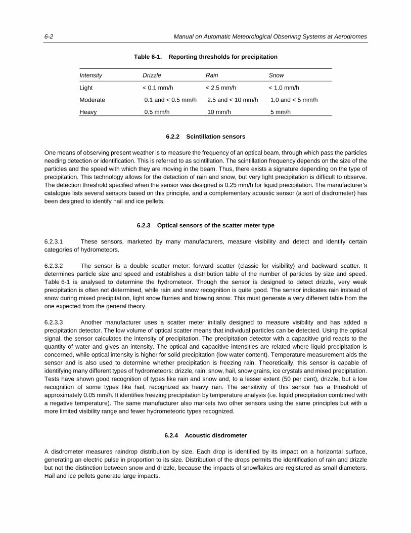
Table 6-1. Reporting thresholds for precipitation
Intensity Drizzle Rain Snow
Light < 0.1 mm/h < 2.5 mm/h < 1.0 mm/h Moderate 0.1 and < 0.5 mm/h 2.5 and < 10 mm/h 1.0 and < 5 mm/h Heavy 0.5 mm/h 10 mm/h 5 mm/h
6.2.2 Scintillation sensors One means of observing present weather is to measure the frequency of an optical beam, through which pass the particles needing detection or identification. This is referred to as scintillation. The scintillation frequency depends on the size of the particles and the speed with which they are moving in the beam. Thus, there exists a signature depending on the type of precipitation. This technology allows for the detection of rain and snow, but very light precipitation is difficult to observe. The detection threshold specified when the sensor was designed is 0.25 mm/h for liquid precipitation. The manufacturer’s catalogue lists several sensors based on this principle, and a complementary acoustic sensor (a sort of disdrometer) has been designed to identify hail and ice pellets.
6.2.3 Optical sensors of the scatter meter type 6.2.3.1 These sensors, marketed by many manufacturers, measure visibility and detect and identify certain categories of hydrometeors. 6.2.3.2 The sensor is a double scatter meter: forward scatter (classic for visibility) and backward scatter. It determines particle size and speed and establishes a distribution table of the number of particles by size and speed. Table 6-1 is analysed to determine the hydrometeor. Though the sensor is designed to detect drizzle, very weak precipitation is often not determined, while rain and snow recognition is quite good. The sensor indicates rain instead of snow during mixed precipitation, light snow flurries and blowing snow. This must generate a very different table from the one expected from the general theory. 6.2.3.3 Another manufacturer uses a scatter meter initially designed to measure visibility and has added a precipitation detector. The low volume of optical scatter means that individual particles can be detected. Using the optical signal, the sensor calculates the intensity of precipitation. The precipitation detector with a capacitive grid reacts to the quantity of water and gives an intensity. The optical and capacitive intensities are related where liquid precipitation is concerned, while optical intensity is higher for solid precipitation (low water content). Temperature measurement aids the sensor and is also used to determine whether precipitation is freezing rain. Theoretically, this sensor is capable of identifying many different types of hydrometeors: drizzle, rain, snow, hail, snow grains, ice crystals and mixed precipitation. Tests have shown good recognition of types like rain and snow and, to a lesser extent (50 per cent), drizzle, but a low recognition of some types like hail, recognized as heavy rain. The sensitivity of this sensor has a threshold of approximately 0.05 mm/h. It identifies freezing precipitation by temperature analysis (i.e. liquid precipitation combined with a negative temperature). The same manufacturer also markets two other sensors using the same principles but with a more limited visibility range and fewer hydrometeoric types recognized.
6.2.4 Acoustic disdrometer A disdrometer measures raindrop distribution by size. Each drop is identified by its impact on a horizontal surface, generating an electric pulse in proportion to its size. Distribution of the drops permits the identification of rain and drizzle but not the distinction between snow and drizzle, because the impacts of snowflakes are registered as small diameters. Hail and ice pellets generate large impacts.

Chapter 6. Present Weather 6-3
6.2.5 Optical disdrometer An optical disdrometer detects the size, number and fall speed of drops as they pass a light barrier (Figure 6-1 refers). Each type of particle (drizzle, rain, snow, hail, etc.) has a signature in a two-dimensional table (size and speed), so that the type of precipitation can be recognized. There are at least two recent sensors of this type on the market.
Figure 6-1. Optical disdrometer
6.2.6 Microwave radar sensor One State has developed a bistatic X-ray radar sensor, pointing vertically. The signal emitted is reflected by particles and undergoes a Doppler shift according to the fall speed: weak for snow, stronger for rain. Signal intensity depends on the number and type of particles. As a result, the sensor can distinguish rain and snow, but identifying drizzle is a more delicate matter.
6.2.7 Ice accretion sensor This sensor detects the presence of a layer of ice or frost on a vibrating rod, the resonance frequency of which varies accordingly. The rod is heated once its frequency falls below a defined threshold. This sensor is used in almost all Automated Surface Observing Systems (ASOS) in the United States to detect ice in precipitation. It is also used to detect conditions of freezing drizzle, which eludes detection by the present weather optical sensor.
6.2.8 Temperature sensor One development under way is the measurement of the thermal energy needed to melt solid precipitation. Such a sensor would permit the detection and identification of hail or small hail in certain circumstances: the necessity of melting a hydrometeor when the ambient temperature is above 5°C is a good indication of the presence of hail or small hail. The capacities of such a sensor have still to be proven.
6.2.9 Precipitation detectors There are several models that fall into two main categories: optical (detection of particles passing through a light beam); and grid (detection of water on a surface, modifying an electric resistance or capacity). These detectors cannot identify

6-4 Manual on Automatic Meteorological Observing Systems at Aerodromes
precipitation type, but they can be sufficient for sites not subject to certain types of hydrometeor; for example, it is not necessary to identify snow in tropical regions.
6.2.10 Lightning detectors There are several sensors that detect lightning within a 50-km radius, using the magnetic and electrostatic signature of the lightning. By assessing the distance and direction of the lightning, these sensors can provide local information on thunderstorms. An alternative to a local sensor is a lightning detection network.
6.3 INSTRUMENT LIMITATIONS The current instrument limitations in identifying present weather are as follows: a) for most sensors, the identification of rain and snow is correct in 90 per cent of cases, or greater where
the precipitation intensity is higher; b) only some sensors can identify drizzle, but performance is low (50 per cent of cases at best); c) no sensor really identifies hail; d) mixed precipitation is rarely reported. It is seen as either rain or snow; e) where intensities are very low (< 0.1 mm/h), precipitation type is not well identified. The code
“unidentified precipitation (UP)” is often used and is preferable to an identification error; f) a compromise must be reached between the detection threshold and the rate of false alarms (detection
of non-existent phenomena); even the most “sensitive” sensors are sometimes subject to false alarms. It is therefore important to determine the most practical detection threshold. For aeronautical use, it is not necessary to detect very weak intensities (e.g. < 0.1 mm/h), except for freezing precipitation for which the threshold of 0.02 mm/h is recommended;
g) snow intensity is not always well reported; and h) optical systems are sensitive to pollution and require regular maintenance, especially if they are near the
sea.
6.4 ALGORITHMS AND REPORTING
6.4.1 General 6.4.1.1 The processing of the physical signals measured is done by the sensor itself. Detailed algorithms constitute manufacturer’s know-how and are more or less documented, depending on the manufacturer. They sometimes use the temperature to correct or establish the diagnostic of present weather. That can serve a double purpose with the complementary algorithms of an external processing system, in which case it is important that the internal processing be known, so that the overall system functions well.

Chapter 6. Present Weather 6-5
6.4.1.2 Potentially, the final diagnostic of present weather could be greatly improved with a combination of different sensors or parameters. The use of air temperature is the most obvious example, but there are other useful parameters or other inter-parametric correlations. Thus, supplementary, more “classical” sensors, such as temperature measurements, can be installed and used. Data combination algorithms permit the identification of complementary types of present weather or the correction of initial diagnostics sent by the present weather sensor. In this case, some algorithms can be specific to the sensor used and its known faults. 6.4.1.3 Many States and/or meteorological services develop and use such algorithms. It is not easy to gain an overview as few of these algorithms are clearly documented and sometimes they are regarded as having commercial value. At present, it is not possible to standardize these algorithms, nor to cite them. 6.4.1.4 Some studies have shown the usefulness of temperature measurement instruments (not protected by a shelter) placed at two levels above the ground, e.g. at +10 cm and +50 cm, called T+10 and T+50. When there is no precipitation, these two temperatures are often different, because there is a temperature gradient above the ground: at night, with a clear sky, the ground is cooler and therefore T+10 is cooler than T+50; by day, with a clear sky, the ground is warmer and therefore T+10 is warmer than T+50. However, in the presence of fog or precipitation, these two temperatures are subject to the same atmospheric conditions, which minimize the differences in temperature that can exist between the two measurements. This fact can be used, but the absence of a temperature gradient does not mean that there is fog or precipitation. For the same reasons, the comparison with air temperature (Tair) is also useful. 6.4.1.5 Examples of algorithms regarding present weather detection (6) and identification (7) are given in Appendix A.
6.4.2 Detection thresholds 6.4.2.1 Automatic systems can detect hydrometeors, the detection threshold depending on the initial specifications of the system and sensors used. A defined detection threshold does not exist. 6.4.2.2 The initial specifications of the ASOS in the United States were around 0.25 mm/h. A recommendation by the WMO Commission for Instruments and Methods of Observation (CIMO) defines a 0.02 mm/h threshold as a lower limit used to indicate traces of precipitation (trace between 0.02 and 0.2 mm/h). A commonly used averaging interval for the abovementioned intensities is 10 minutes. 6.4.2.3 For aeronautical needs, the useful threshold limit has still to be defined. A 0.02 mm/h threshold is probably appropriate for freezing precipitation; such a low threshold is probably not required for other types of precipitation. Furthermore, an intensity described as “light” would cover a very wide dynamic range (0.02 mm/h to 2.5 mm/h), with a very variable operational importance. The term “light” already implies that the phenomenon has a minor influence, so an intensity of 0.02 mm/h perhaps has no effect. The disadvantage to an automatic system with a very low detection threshold is its difficulty in identifying the hydrometeor in such conditions. The use of the abbreviation “UP” proves useful here. Experience with the first automatic systems installed indicates that a 0.2 mm/h threshold could be acceptable, except for freezing precipitation, for which 0.02 mm/h would be recommended.
6.4.3 Identification of drizzle (DZ) Some systems can distinguish drizzle from rain, but current sensors are reliable only 50 per cent of the time. This could be improved with complementary algorithms, but little progress is expected in the near future. Another difficulty in identifying drizzle is simply its detection, since drizzle droplets are very small and thus hard to detect by some sensors.
6.4.4 Identification of rain (RA) and snow (SN) Many sensors accurately identify rain and snow, except where intensities are very low (< 0.1 or 0.2 mm/h). Whenever there is too much uncertainty, it is preferable to use the abbreviation UP.

6-6 Manual on Automatic Meteorological Observing Systems at Aerodromes
6.4.5 Identification of snow grains (SG), ice pellets (PL) and ice crystals (IC)
Very few present weather sensors and hence very few automatic systems today are able to recognize these types of hydrometeors. Those that can (or claim to be able to) are not very reliable. Also, comparisons show that the more types of hydrometeor a sensor can detect, the more confusion there is between the types. If they are not identified individually, they will often be reported as snow.
6.4.6 Identification of hail (GR), small hail and/or snow pellets (GS)
Studies show that sensors have great difficulty identifying hail and snow pellets. In many cases, the precipitation is identified as heavy rain instead. The problem lies with the way in which optical and/or radar signals are used in the identification process. In order to obtain greater accuracy in this identification, special sensors are needed. Work is under way to develop new methods based on acoustic and thermal techniques.
6.4.7 Identification of fog (FG), mist (BR), haze (HZ) and smoke (FU)
6.4.7.1 Visibility sensors correctly identify fog (visibility less than 1 000 m) and mist (visibility between 1 000 and 5 000 m). Caution has to be exercised, however, since the visibility to be considered is the visibility for aeronautical purposes as defined in Chapter 1 of Annex 3. 6.4.7.2 The presence of fog must be confirmed by a high relative humidity of at least 95 per cent (not 100 per cent to account for the uncertainty of the measurement) to avoid the use of the abbreviation FG when the visibility is reduced by heavy rain or, especially, snow. The presence of RA or SN in this case should be clearly identified by the present weather sensor because their intensity would assist in determining the presence of fog (or otherwise). 6.4.7.3 The presence of mist must be confirmed by a high relative humidity of at least 80 per cent. If the relative humidity is lower, it is haze, coded as HZ. Visibility can temporarily drop below 5 000 m in the case of precipitation or smoke. A characteristic of mist or haze is its good temporal stability, at least over a 10- to 30-minute period. This might cause visibility to vary, but slowly and continuously, without major fluctuations. Major fluctuations indicate the presence of precipitation or smoke. A criterion for the stability of visibility is recommended for mist and haze. Conversely, when there is no precipitation and visibility fluctuates, smoke might well be present and should be reported. However, one must always be aware that the capacity of an automatic system to report very local phenomena like smoke is limited by selective visibility measurements. Smoke will not be seen unless it passes the sensor. 6.4.7.4 The representative visibility of the aerodrome should be used to identify fog, mist or haze. If there are several scatter meters, multiple visibility measurements should be used to identify (localized) fog patches (BCFG) or partial fog (PRFG) covering a substantial part of the aerodrome.
6.4.8 Identification of sand (SA), dust (DU), volcanic ash (VA), dust sand whirls (PO),
funnel cloud (FC), duststorm (DS), and sandstorm (SS) Current automatic systems cannot report these phenomena. For a duststorm (DS) or sandstorm (SS), coding could be arranged using a combination of low visibility (e.g. < 1 000 m), low relative humidity (e.g. < 50 per cent) and high wind speed (e.g. average wind over ten minutes > 15 m/s (30 kt)). Studies could be done showing the correlation between these parameters and the occurrence of DS or SS, using data gathered on site subject to these conditions.

Chapter 6. Present Weather 6-7
6.4.9 Identification of a squall (SQ) A squall is defined by a sudden increase in wind speed lasting at least one minute and sometimes several. It is often accompanied by a wind change and a sudden variation in atmospheric pressure. In practice, squalls can be detected by comparing the spot wind with the average wind over two minutes to see whether there has been a certain increase (e.g. at least 8 m/s (16 kt)), lasting at least one minute; this prevents simple gusts from being confused with squalls. If several wind sensors are installed, the data from each should be analysed to detect a squall.
6.4.10 Identification of thunderstorm (TS) 6.4.10.1 The presence of thunderstorms can be determined by a local lightning detector or by using a lightning sensor network. Development work is ongoing to ensure that the information from the network can be utilized in the local observation system at the aerodrome. 6.4.10.2 The descriptor TS is used when a thunderstorm is detected at an aerodrome, with an indication of precipitation, if present. Joint use of the abbreviations TS and shower (SH) in the same group is not possible; priority should be given to TS over SH. Objective distance assessment is possible with lightning detectors and networks. 6.4.10.3 In local routine and special reports and in METAR/SPECI, thunderstorm shall be reported when thunder is heard or lightning is detected at the aerodrome during the 10-minute period preceding the time of observation but no precipitation is observed at the aerodrome. An example of thunderstorm reporting based on observational data from a lightning detection system and weather radar is given under “Present weather identification (7)” in Appendix A.
6.4.11 Identification of shower (SH) There is no objective or mathematical definition for showers in terms of precipitation rates. To be able to identify showers, it is necessary to analyse the intensity of precipitation over a given period, for example, one hour. During this time, periods of precipitation must be isolated from periods without precipitation. Another method to determine the presence of showers is to analyse the spatial differences in intensities when more than one sensor is used on an aerodrome. Further identification of showers can be made using the assessment of the presence of cumulonimbus clouds (see Chapter 7).
6.4.12 Identification of freezing rain (FZRA) and freezing drizzle (FZDZ)
Freezing rain or freezing drizzle often occur when the air temperature is below zero. Liquid precipitation is almost always freezing when Tair < –0.5°C. This is a simple and relatively reliable way of identifying the freezing nature of precipitation, on condition that the precipitation was detected and properly identified as liquid. For very light precipitation, an icing sensor that reacts to a small amount of ice is required. Whether or not to install this sensor in an automatic system depends on the frequency of freezing phenomena.
6.4.13 Identification of blowing snow (BLSN) Many sensors analyse particles that pass through an analysis volume. Blowing snow can be confused with snow or another type of hydrometeor since it is moving faster than usual. The behaviour of the sensor depends on its design and physical principles. One State is known to have developed an algorithm to detect BLSN.
6-8 Manual on Automatic Meteorological Observing Systems at Aerodromes
6.4.14 Identification of low drifting (DR) and shallow (MI) phenomena
Present weather and/or visibility sensors are usually installed at a height greater than 2 m. Low-lying phenomena (i.e. phenomena occurring below the height of the sensor) cannot be detected, and “low drifting” (DR) or “shallow” (MI) phenomena characteristics are not usually available with an automatic system. This would require specific instruments or the installation of sensors at a height less than 2 m. The detection of such phenomena has not yet been deemed important enough to justify an investment in specific instruments.
6.4.15 Identification of patches (BC) and partial (PR) (applied to fog)
6.4.15.1 The descriptors BC and PR apply to fog and should not be used alone. In the presence of fog patches, fog is not homogeneous and there is a local temporal variability in visibility. For example, if the visibility analysis at one point shows the presence of at least two visibility episodes below 1 000 m, separated by at least five minutes, the abbreviation BC should probably be used. If there are many visibility sensors at the airport, all available sensors can look for fog episodes to increase the probability of detecting fog patches. 6.4.15.2 The abbreviation PR (partial) can only be reported if there are many visibility sensors at the airport and if some of the sensors indicate stable visibility below 1 000 m. Stability is necessary to distinguish fog patches. The stability can be evaluated by the presence of no fog episodes or a single fog episode (over a one-hour period, for example) per sensor.
6.4.16 Use of unidentified precipitation (UP) 6.4.16.1 Not all weather elements of the METAR/SPECI code can be reported by automatic systems. However, it is likely that the automatic system will be able to identify that there is a precipitation event occurring, using a combination of visibility, temperature and present weather sensors, but may be unable to resolve the type. In this situation, unidentified precipitation may be reported using the abbreviation UP. 6.4.16.2 The ability of an automatic sensor to identify a particular type of precipitation will depend upon the technology that is in use. A list is given below of the weather phenomena that may be reported as UP: — drizzle (DZ) — ice crystals (IC) — ice pellets (PL) — snow grains (SG) — hail (GR) — small hail and/or snow pellets (GS) — dust (DU) — duststorm (DS) — sand (SA) — sandstorm (SS).

Chapter 6. Present Weather 6-9
6.4.17 Identification of the intensity of precipitation Three intensity levels are defined for hydrometeors. Present weather sensors can measure the intensity of the hydrometeors they detect. This intensity is indicated by sensors in mm/h, and sometimes as light, moderate or heavy (Table 6-1 refers), which is only the result of an intensity test in mm/h in relation to thresholds integrated in the sensor. Intensity often varies significantly in time, so it is necessary to filter information before determining the intensity level. A WMO Commission for Instruments and Methods of Observation (CIMO) working group proposed using the mean of the three maximum intensities over the last 10 minutes (intensities being available every minute).
6.4.18 Identification of vicinity (VC) With an automatic system using local instruments at the aerodrome, phenomena occurring in the vicinity (using the abbreviation VC) cannot be reported, except for a TS when it can be identified by a lightning detection instrument capable of indicating its distance. The only way of reporting other types of present weather phenomena occurring in the vicinity would be to install additional sensors, where practicable, in the vicinity of the airport. As automatic systems are often installed at small aerodromes, an investment in multiple sensors around the aerodrome cannot be justified in most cases. The abbreviation VC is used when a phenomenon is detected outside the aerodrome at distances defined to be between approximately 8 and 16 km from the aerodrome reference point. The precise range to be applied for the reporting of VC is to be determined locally in consultation with the civil aviation authority and will be dependent on the actual size of the aerodrome complex.
6.4.19 Combination of algorithms All data combination algorithms are usually installed in a central computer of the observation system. The different combinations can be complex. There are several ways of combining the different algorithms: — A classic approach: a series of tests leading to a diagnostic and coding. — A combination approach: a combination of many individual algorithms to which weights are given, for
cases where algorithms yield different diagnostics. — A “fuzzy logic” approach (a technical solution to the problem): a mathematical method that utilizes
previous diagnostic experience to identify the appropriate weights to be given to particular algorithms in a variety of different situations. Numerous texts exist in the application of fuzzy logic techniques; thus, the topic will not be covered in detail in this manual.
6.4.20 Variability of parameters 6.4.20.1 Most present weather phenomena do not vary significantly in time, over an interval of a few minutes. In cases of low intensity, the internal algorithms of the system examine the diagnostics over the last few minutes to confirm or reject them (and possibly code UP in case of doubt). 6.4.20.2 However, precipitation intensities often vary significantly in time. It is recommended that the data be smoothed during the last 10 minutes. Temporal variations in intensity can also be used to determine the nature of downpours. 6.4.20.3 Apart from some phenomena such as fog, rain, hail, small hail and smoke, present weather is very often homogeneous at the airport, and it is not necessary to install many sensors at different locations. Because of its operational significance, visibility is a specific case which can justify the installation of multiple sensors, which can be used to increase the detection reliability of fog and to report on possible associated characteristics (patches (BC) and partial (PR)).
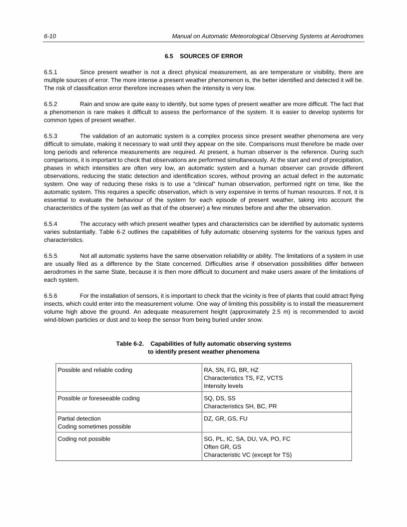
6-10 Manual on Automatic Meteorological Observing Systems at Aerodromes
6.5 SOURCES OF ERROR 6.5.1 Since present weather is not a direct physical measurement, as are temperature or visibility, there are multiple sources of error. The more intense a present weather phenomenon is, the better identified and detected it will be. The risk of classification error therefore increases when the intensity is very low. 6.5.2 Rain and snow are quite easy to identify, but some types of present weather are more difficult. The fact that a phenomenon is rare makes it difficult to assess the performance of the system. It is easier to develop systems for common types of present weather. 6.5.3 The validation of an automatic system is a complex process since present weather phenomena are very difficult to simulate, making it necessary to wait until they appear on the site. Comparisons must therefore be made over long periods and reference measurements are required. At present, a human observer is the reference. During such comparisons, it is important to check that observations are performed simultaneously. At the start and end of precipitation, phases in which intensities are often very low, an automatic system and a human observer can provide different observations, reducing the static detection and identification scores, without proving an actual defect in the automatic system. One way of reducing these risks is to use a “clinical” human observation, performed right on time, like the automatic system. This requires a specific observation, which is very expensive in terms of human resources. If not, it is essential to evaluate the behaviour of the system for each episode of present weather, taking into account the characteristics of the system (as well as that of the observer) a few minutes before and after the observation. 6.5.4 The accuracy with which present weather types and characteristics can be identified by automatic systems varies substantially. Table 6-2 outlines the capabilities of fully automatic observing systems for the various types and characteristics. 6.5.5 Not all automatic systems have the same observation reliability or ability. The limitations of a system in use are usually filed as a difference by the State concerned. Difficulties arise if observation possibilities differ between aerodromes in the same State, because it is then more difficult to document and make users aware of the limitations of each system. 6.5.6 For the installation of sensors, it is important to check that the vicinity is free of plants that could attract flying insects, which could enter into the measurement volume. One way of limiting this possibility is to install the measurement volume high above the ground. An adequate measurement height (approximately 2.5 m) is recommended to avoid wind-blown particles or dust and to keep the sensor from being buried under snow.
Table 6-2. Capabilities of fully automatic observing systems to identify present weather phenomena
Possible and reliable coding RA, SN, FG, BR, HZ Characteristics TS, FZ, VCTS Intensity levels
Possible or foreseeable coding SQ, DS, SS Characteristics SH, BC, PR
Partial detection Coding sometimes possible
DZ, GR, GS, FU
Coding not possible SG, PL, IC, SA, DU, VA, PO, FC Often GR, GS Characteristic VC (except for TS)
Chapter 6. Present Weather 6-11
6.6 CALIBRATION AND MAINTENANCE 6.6.1 Sensors must be maintained according to manufacturers’ recommendations. Regular maintenance usually consists of cleaning the outside, especially for optical sensors. Monitoring and/or calibration recommendations for optical sensors that use a backscatter light are usually the same as for scatter meters that measure visibility (see Chapter 4). 6.6.2 One of the problems when calibrating present weather sensors is the difficulty of simulating hydrometeors. The stability of a characteristic of the sensor depends on its design. One monitoring method is to make localized comparisons with a local observer throughout the life of the system, or to establish correlations or comparisons with neighbouring observation stations during slow-moving and widespread weather events.
6.7 MEASUREMENT LOCATIONS 6.7.1 Annex 3 specifies that present weather information should be representative of conditions at the aerodrome and, for certain specified present weather phenomena, in its vicinity. 6.7.2 In the case of automatic observations, it is acceptable for an observation to be made at a single point, chosen as the most representative of the aerodrome and/or usually located to provide easy access for installation, maintenance and data transmission, such as the meteorological enclosure. For information on fog and mist, the automatic system must use all sensors available at the aerodrome.
___________________

7-1
Chapter 7
CLOUDS
7.1 INTRODUCTION 7.1.1 Like visibility and RVR, the cloud amount, the cloud type, and height of cloud base must be reported as they greatly affect operations. For example, too low a cloud base can downgrade a runway or airport because it has a direct influence on the pilot’s view of the runway. Cumulonimbus (CB) or towering cumulus (TCU) are convective clouds potentially dangerous to aircraft owing to the associated wind shear which can affect landings and take-offs. 7.1.2 Cloud amount is described using four abbreviations: few (FEW), scattered (SCT), broken (BKN) and overcast (OVC).
7.2 MEASUREMENT METHODS
7.2.1 Height of cloud base 7.2.1.1 A ceilometer is the only automatic sensor currently capable of measuring the height of a cloud base. All recent models use a laser diode as a light source. Ceilometers measure precisely the cloud base directly above the sensor. An analysis of successive measurements provides an evaluation of the cloud layers with the same regularity, day and night. 7.2.1.2 A light pulse is directed upwards and part of the light power is reflected or backscattered by the different aerosols and particles in the atmosphere. A very fast electronic detector measures the return signal for different successive instants. Each instant corresponds to a distance equal to the time between emission of the light (pulse) and its reception, divided by the speed of light and again divided by two (emission and return). The system determines a backscatter profile of the signal, which is how a ceilometer works. 7.2.1.3 The power from a light pulse is limited by technology and especially by safety standards, i.e. light pulses must not be dangerous to the human eye. The power of the backscattered signal is therefore very low and barely different from background light. It is therefore necessary to multiply the number of laser pulses (usually over 10 000) to increase the signal/noise ratio and to obtain a useable backscatter profile. 7.2.1.4 The first ceilometers were designed solely for aeronautical purposes and had a measurement range of 30 m (100 ft) or 45 m to 1 500 m (150 ft to 5 000 ft). More recent ceilometers have a wider measurement range, from 30 m (100 ft) or less to 6 000 m (20 000 ft) or more. The measurement range meets all the aeronautical requirements since only clouds with the height of cloud base below 1 500 m (5 000 ft) (or below the highest minimum sector altitude, whichever is greater) are considered to be of operational significance and need to be reported. The better performance of instruments and improvements in the way signals are processed have resulted in increased efficiency.
7-2 Manual on Automatic Meteorological Observing Systems at Aerodromes
7.2.2 Cloud amount 7.2.2.1 The United States, with ASOS, has developed an algorithm that makes it possible to calculate the cloud amount by analysing the indications of the height of cloud bases over the last 30 minutes. This method and its limits are described in 7.3. 7.2.2.2 There are also prototype cloud amount sensors based on the use of one or more infrared radiometers pointed successively towards different areas of the sky to determine the radiative temperature. This temperature is lower when the sky is clear and higher when clouds are present; the radiative temperature of clouds decreases with altitude. It is, however, necessary to take the ambient temperature or real temperature profile into account. A cloud at 0°C can be close to the ground or at 3 000 m (10 000 ft), depending on the season and location. Such sensors cannot precisely indicate the height of cloud bases. However, they have the capability of indicating cloud amount without the disadvantage of the algorithm associated with a ceilometer, which can “see” only clouds passing above the ceilometer. They can detect the arrival or extent of a cloud layer right above a ceilometer and therefore can complete the information the ceilometer provides. 7.2.2.3 There are also sensors that “photograph” the image of the sky reflected on a hemispherical dome or through a fish-eye optic. Analysing the image can make it possible to detect the presence of clouds and to calculate their amount, but this method works only during daytime in visible light. At night, it would be necessary to use infrared instruments looking directly at the sky. This is similar to the method discussed in 7.2.2.2.
7.2.3 Cloud type — Detection of cumulonimbus (CB) and towering cumulus (TCU) clouds
7.2.3.1 CB and TCU clouds are identified visually and sometimes acoustically. A cumulonimbus can be buried in a cloud mass, without being directly identifiable by a human observer. Lightning and/or thunder indicate the presence of CB clouds. 7.2.3.2 A weather radar detects the presence of precipitation (and sometimes even clouds) and quantifies its intensity. Intense or deep convective cloud cells are visible and result in high reflectivity levels. A proposal is being examined by the WMO Commission for Instruments and Methods of Observation (CIMO) to define CB and TCU clouds or, more precisely, convective clouds using reflectivity levels. A disadvantage of this method is that high levels of reflectivity can also exist during heavy, non-convective precipitation, without the presence of CB and TCU clouds. The combination of radar images with infrared satellite images can fine-tune the diagnostic, since CB and TCU clouds have a large vertical extent; thus, the temperature at their tops is low. 7.2.3.3 Radar and satellite images are commonly used by meteorological forecasters. Products adapted to convective phenomena are becoming available to aeronautical users in certain countries. Development is under way in many countries to extract information on convective clouds from radar and satellite images and integrate it into METAR/SPECI and local reports. A definition of the area around the airport, in which CB/TCU clouds must be indicated, is also necessary. This area should perhaps be related to the area where a thunderstorm might be detected (TS or VCTS). Since a definition does not exist at present, it is possible for the presence of CB clouds to be indicated by a human observer when he sees lightning, even if far away (a distance up to 100 km is possible at night). 7.2.3.4 There are local sensors and/or networks that detect lightning in a defined area corresponding to the zone affected by TS and VCTS. Lightning indicates the presence of CB clouds. Unfortunately, there are many cases of false alarms which rendered this method somewhat unreliable. 7.2.3.5 There are also electric-field sensors (field generators) whose wide variations can indicate that a thunderstorm is approaching, but there are no reliable automatic algorithms that link the electric field to the presence of CB clouds.

Chapter 7. Clouds 7-3
7.3 ALGORITHMS AND REPORTING
7.3.1 Determining cloud layers using a ceilometer 7.3.1.1 Many algorithms developed by meteorological authorities and/or system designers are used throughout the world to calculate cloud layers using a ceilometer. It is difficult to standardize algorithms precisely, but all algorithms use the same method of calculation, developed by the United States with ASOS. This method is described below. 7.3.1.2 A ceilometer usually provides data every 15 or 30 seconds. Individual data on the height of cloud base (or lack of cloud base) are used over a period of 30 minutes. To accelerate detection of a recent change, the last 10 minutes are taken into account with a double weight in the algorithm. The basic principle of the algorithm is that the clouds passing above the ceilometer give a good indication of the cloud amount. The 30-minute period is a compromise between an integration that is long enough to be representative and short enough not to introduce a smoothing and a late detection of a variation that is significant. Some countries use a longer period of one hour. 7.3.1.3 Individual detections are classified in intervals of 30, 60 or 150 m (100, 200 or 500 ft) depending on the height, and they form a set of classes with a width and number of impacts within the width. There are usually several classes with a non-zero number of impacts after this process, and the number must be reduced. Classification is made according to height. 7.3.1.4 Examples of algorithms regarding cloud layers (8) are given in Appendix A.
7.3.2 Determining cloud layers using multiple ceilometers If the aerodrome has ceilometers located near each end of the runway, cloud layers must be calculated for each and included in local reports, where appropriate. For METAR/SPECI, the observation must be representative of the aerodrome and its vicinity although it is acceptable for the cloud observation to be made at a single point, chosen as the most representative of the aerodrome. Where there are multiple ceilometers installed on the aerodrome, it may be possible to integrate the measurements from the ceilometers in an algorithm such as described above, which will handle a greater number of base measurements.
7.3.3 Detecting the presence of cumulonimbus (CB) and towering cumulus (TCU) clouds
7.3.3.1 A ceilometer, the only automatic sensor currently capable of measuring the height of a cloud base, cannot identify CB or TCU clouds. This identification can therefore only be done from a secondary source of observation (see 7.4.4 for further details). If this source is a human observer, the observation system’s central computer must make it possible to enter cloud layers or modify layers calculated automatically and add the indication CB or TCU to some of these layers. 7.3.3.2 If this source is an automatic system, the information available probably indicates the presence or absence of deep convective clouds, or CB or TCU clouds, without indicating the associated height and probably without indicating cloud amount. This is the case, for example, when the source is a radar image analysis or the identification of CB clouds resulting from the presence of lightning. In this case, it is difficult to give the indication CB or TCU to an existing cloud group or to associate it with a cloud amount and height.
7.3.4 Variability of parameters 7.3.4.1 Spatial and temporal variability of cloud parameters greatly depend on the meteorological situation and sometimes on the site.
7-4 Manual on Automatic Meteorological Observing Systems at Aerodromes
7.3.4.2 When the sky is completely clear or completely overcast, there are no temporal or spatial changes. A single ceilometer on a site is more than enough, and an algorithm to calculate cloud layers as described in Appendix A yields excellent results, when compared to a human observer. 7.3.4.3 When the sky is partially covered by cumulus, temporal variability above a given point (such as where a ceilometer is installed) is high. In fact, this is the variability used by the algorithm to calculate the number of cloud layers. Evaluated over a 30-minute period, spatial variability is usually low throughout the aerodrome, except if there are marked terrain effects on the site. This can be the case with terrain contours nearby or with airports located on the shoreline where clouds often present a clear line between the shore and the water. 7.3.4.4 There are cases where there can be significant differences in cloud amount or height above different points of the aerodrome, for example, as a result of terrain effects. These cases do not occur often, except at certain sites that can require specific instruments. Rare cases occur over a short period during a transition phase, which is why the algorithm gives a double weight to the last 10 minutes. 7.3.4.5 Therefore, except for specific sites identifiable by their climate, an automatic observation based on a single ceilometer is often representative of the aerodrome. This does not detract from the importance of having a ceilometer at each end of the runway in use, for conditions where cloud amount and height are not homogeneous at the airport and in its vicinity: this condition may be rare but is of importance to aircraft operations.
7.4 SOURCES OF ERROR
7.4.1 Height of cloud base 7.4.1.1 The information given by a ceilometer is currently the best estimate of the true height of cloud bases. A ceilometer is very precise when there are clouds with a well-defined base or a homogeneous cloud layer. In fact, no other instrument performs better. This makes it difficult to truly evaluate the uncertainty of measurements. Comparing different ceilometer models is one way of evaluating the uncertainty of measurements, without really knowing the true value when there are differences. In addition to differences in the reported altitude, a comparison can reveal differences in cloud detection capability, especially depending on the height of the cloud base and meteorological conditions. 7.4.1.2 Uncertainty is greater in cases of diffuse cloud bases or heavy precipitation. In this case, the ceilometer sometimes indicates a vertical visibility that is often close to the height of a cloud base measured before or after. With precipitation, if the indication is of a cloud base, the height indicated is usually less than the actual base.
7.4.2 Vertical visibility 7.4.2.1 Some ceilometers provide vertical visibility in certain circumstances (similar to the profile of the backscattered signal). The validity of the vertical visibility value is difficult to establish. 7.4.2.2 First, the notion of vertical visibility is not clearly defined in Annex 3. In the case of vertical visibility reported in place of the height of a cloud base, the vertical visibility value is often low (between 30 m (100 ft) and 210 m (700 ft)), and the decision to take into account (or not) a light source to calculate visibility is particularly important. For such values, there exists approximately a factor of 3 between the visibility based on the contrast and visibility using light sources. 7.4.2.3 Second, it is very difficult for a human observer to estimate vertical visibility; vertical marks are required but do not exist (except at the foot of a tower). An aircraft could be a mark, in front of the runway threshold, but it would be a moving mark that could not be anticipated (since vertical visibility changes slowly). If an observer uses a vertical tower, he usually does so at a slant and the assessment is therefore compromised.
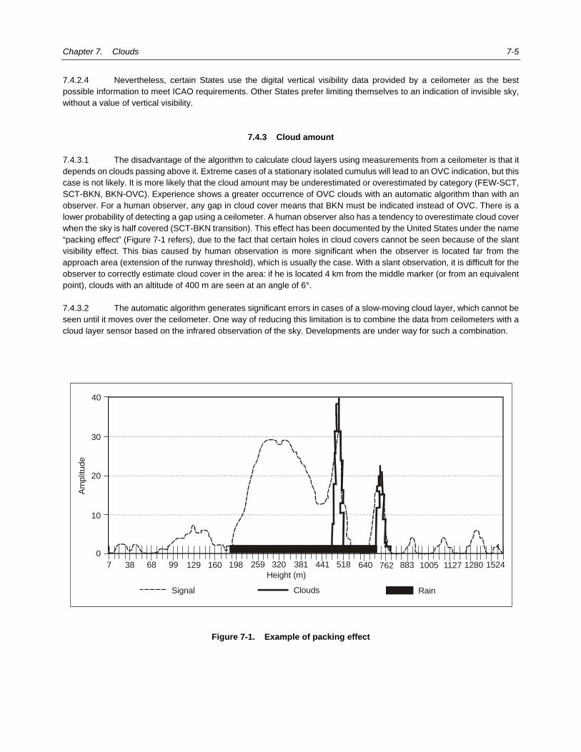
Chapter 7. Clouds 7-5
7.4.2.4 Nevertheless, certain States use the digital vertical visibility data provided by a ceilometer as the best possible information to meet ICAO requirements. Other States prefer limiting themselves to an indication of invisible sky, without a value of vertical visibility.
7.4.3 Cloud amount 7.4.3.1 The disadvantage of the algorithm to calculate cloud layers using measurements from a ceilometer is that it depends on clouds passing above it. Extreme cases of a stationary isolated cumulus will lead to an OVC indication, but this case is not likely. It is more likely that the cloud amount may be underestimated or overestimated by category (FEW-SCT, SCT-BKN, BKN-OVC). Experience shows a greater occurrence of OVC clouds with an automatic algorithm than with an observer. For a human observer, any gap in cloud cover means that BKN must be indicated instead of OVC. There is a lower probability of detecting a gap using a ceilometer. A human observer also has a tendency to overestimate cloud cover when the sky is half covered (SCT-BKN transition). This effect has been documented by the United States under the name “packing effect” (Figure 7-1 refers), due to the fact that certain holes in cloud covers cannot be seen because of the slant visibility effect. This bias caused by human observation is more significant when the observer is located far from the approach area (extension of the runway threshold), which is usually the case. With a slant observation, it is difficult for the observer to correctly estimate cloud cover in the area: if he is located 4 km from the middle marker (or from an equivalent point), clouds with an altitude of 400 m are seen at an angle of 6°. 7.4.3.2 The automatic algorithm generates significant errors in cases of a slow-moving cloud layer, which cannot be seen until it moves over the ceilometer. One way of reducing this limitation is to combine the data from ceilometers with a cloud layer sensor based on the infrared observation of the sky. Developments are under way for such a combination.
Figure 7-1. Example of packing effect
7 38 68 99 1524129 160 198 259 320 381 441 518 640 762 883 1005 1127 12800
10
20
30
40
Ampl
itude
Height (m)
Signal Clouds Rain
7-6 Manual on Automatic Meteorological Observing Systems at Aerodromes
7.4.4 Identification of cumulonimbus (CB) and towering cumulus (TCU) clouds
7.4.4.1 For an observer, the presence of CB clouds can be detected visually (shape of cloud) or deduced from the occurrence of lightning or thunder. A CB cloud buried in a cloud mass can be invisible to an observer and would therefore not be reported. If lightning is visually detected, distant CB clouds can be detected and reported. A human observation has specific characteristics that differ from those of an automatic detection based on the analysis of a radar image. An observer is also often aware of the meteorological situation using radar images, satellites, forecast models, etc. The observer’s expertise can therefore indicate the presence of CB clouds even if they cannot be seen directly from the meteorological station. 7.4.4.2 An automatic identification of CB clouds is essentially based on the surpassing of radar reflectivity thresholds (for example, 44 dBZ), associated with a recognition of location cells. It is therefore necessary to set a maximum distance between the aerodrome reference point and a cell to identify the presence of CB clouds at an airport and in its vicinity. The smaller the distance, the greater the level of CB clouds detected by a human observer and undetected by an automatic analysis. Conversely, if there is a large distance, the level of CB clouds detected by an automatic analysis and not reported by an observer will be higher. The maximum distance at which a human observer is required to report convective clouds is not defined. The definition of vicinity applies to the reporting of present weather including thunderstorms. Therefore, it could be argued that convective clouds (CB and TCU) should be reported only up to a distance of 16 km from the aerodrome reference point. When the height of the cloud base is “low”, e.g. 450 m (1 500 ft), a cloud located at a distance of 16 km is seen at an angle of 1.6° over the horizon, so low that a human observer is unlikely to be able to observe the cloud at a greater distance. However, when CB or TCU are present without other cloud they can be seen at a much greater distance by a human observer. For example a CB with a vertical extent of 7 000 m (21 000 ft) can be seen at several tens of kilometres if it is not embedded or obscured by other clouds. Furthermore, lightning can often be seen at night at distances up to 100 km from the observation site. This means that CB and TCU can be observed by a human observer at distances considerably greater than 16 km. As a result the maximum distance that CB and TCU should be reported is not easy to define. Studies show that a distance of 30 km seems to be a compromise that optimizes the comparability of human and automatic identification. One of these studies shows that 25 per cent of CB clouds reported by an observer (in a METAR/SPECI) are not detected by an automatic system. This can seem very significant, but the same study indicates that half of CB clouds detected by an automatic system are not reported by the observer. Either the automatic system falsely indicates CB clouds for a given area of high reflectivity, or the observer is unable to see one or more CB clouds buried in a cloud mass. Furthermore, the same study reveals that if the distance is increased, the amount of CB clouds not detected by the automatic system is lower, which seems to indicate that in certain circumstances the human observer probably reports CB clouds that are far away. 7.4.4.3 The level of uncertainty of CB cloud detection depends heavily on how a CB cloud observation is defined. If the definition is based on a radar reflectivity level, a radar image (if available) will provide the best possible estimate. 7.4.4.4 Reporting TCU clouds is more uncertain due to the difficulty in identifying a towering cumulus. For an observer, a TCU cloud can be identified only when seen directly. For an isolated TCU cloud, a human observation is easy during the day. For a TCU cloud buried in a cloud mass, the observation is much more difficult from the ground. 7.4.4.5 With an automatic analysis of a radar image, the presence of TCU clouds can be determined by reflectivity levels lower than those of CB clouds. A study showed that a threshold of 33 dBZ is strongly correlated to the diversion of aircraft because of a convective activity and could be a useful threshold for identifying the presence of TCU clouds. However, the detection rate is three times greater than that of a human observation. During heavy precipitation, there is a risk of incorrectly reporting TCU clouds, which are not necessarily related to a convective activity. If the present weather sensor is capable of detecting showers, a heavy shower is likely to indicate the presence of TCU and/or CB. 7.4.4.6 Having detected the presence of CB and/or TCU clouds in the vicinity, using remote sensing equipment, the height of cloud base should be reported as ///.
Chapter 7. Clouds 7-7
7.5 CALIBRATION AND MAINTENANCE 7.5.1 A ceilometer calculates the timing of the backscattered return signal. The stability of distance measurements is therefore linked to the stability of an oscillator, which is a very stable electronic element. The mechanical construction of the instrument guarantees that, except in cases of mechanical shock, the optical axes of emitting and receiving optical beams do not move. 7.5.2 The capability of a ceilometer to detect a cloud is ultimately determined by the sensitivity and stability of the backscatter profile measurement and the data processing algorithms. The sensitivity of the backscatter profile measurement, or the signal to noise ratio, depends upon the design of the optics and electronics of the ceilometer. Stability of the sensitivity is determined mainly by the stability of the light source and the receiver. Many ceilometers monitor these parameters internally. 7.5.3 Optical surfaces must remain clean and clear. A heating mechanism inside the sensor keeps them free from condensation. The protective window must not be contaminated since this could cause spurious signals or attenuate the signal preventing cloud detection. Simply cleaning the surface by hand is enough. Most ceilometers have an automatic blower for reducing degradation of detection capability due to contamination of the window by raindrops or snow. 7.5.4 The lifespan of the laser used depends on the sensor, and the laser often has a shorter life span than the sensor itself; a drop in power will reduce its range. 7.5.5 Ceilometers on the market have the following internal surveillance features: heating, contamination, laser power and indication of the state of sensors when emitting messages. There are usually three states: normal, warning and error, which make it possible to warn the user before automatically invalidating the measurement. It is therefore important for the acquisition system to be designed to handle this diagnostic and maintenance information.
7.6 MEASUREMENT LOCATIONS 7.6.1 Annex 3 recommends that cloud observations for METAR/SPECI be representative of the aerodrome and its vicinity and that local reports be representative of the approach zone. For the approach zone, the best location is the middle marker, or the position equal to 900 or 1 200 m from the runway threshold. In practice, the measurements from the location of the middle marker (or the equivalent location) are acceptable for both local reports and METAR/SPECI. 7.6.2 Installing a ceilometer at the middle marker can sometimes be very costly because of the lack of power, communications and security. In this case, another location must be chosen, such as the runway threshold where other visibility sensors and sometimes RVR sensors are installed.
______________________


8-1
Chapter 8
AIR TEMPERATURE AND DEW-POINT TEMPERATURE
8.1 INTRODUCTION Air and dew-point temperatures are meteorological parameters that are used for determining current meteorological conditions, calculating take-off weight, providing information for passengers, etc. The air and dew-point temperatures must be representative of all the runways although a single value for each parameter is used for the aerodrome. Consequently, the measurements must be taken in an area considered representative of the aerodrome that is not subject to specific fluctuations due to the surrounding environment. The measurements must be taken in an open and naturally ventilated area and the sensors must be protected by a shelter or screen.
8.2 MEASUREMENT METHODS
8.2.1 Temperature sensors 8.2.1.1 Numerous principles of physics, associated with various types of sensors, can be applied to the measurement of temperature. A standard sensor covering the range of air temperature measurements that is strongly recommended due to its numerous benefits is the Pt100 platinum resistance probe, whose most common value of resistance is 100 ohms (Ω) at 0°C. Probes with a resistance of 1 000 Ω at 0°C are also used on occasion. IEC 607511 Class A-compliant probes have an uncertainty factor of less than 0.2°C in the typical measurement range (–40°C to +60°C). 8.2.1.2 As platinum is a corrosion-proof metal, platinum wire probes have excellent stability over time, particularly when the platinum wire is well protected. It is therefore preferable to use a probe with proper mechanical protection. Sensors with corrosion-proof metal casings are used in some States and experience has shown excellent stability, i.e. reliable to within 0.2°C over a 20-year period.
8.2.2 Relative humidity sensors 8.2.2.1 The most economical and widespread method for determining the dew-point temperature consists of measuring the air temperature and its relative humidity. The dew-point temperature is then calculated based on these two parameters. Consequently, it is important that these two measurements be taken within the same screen to reflect the values of the same air sample. The calculation principles and recommended formulas are described in detail in the WMO Guide to Meteorological Instruments and Methods of Observation (WMO–No. 8). 8.2.2.2 The majority of relative humidity sensors in use are capacitive hygrometers. They have a conductive layer covered with an organic substance and a metallic layer thin enough to be porous to water vapour. The resulting electric capacity fluctuates in accordance with the dielectric constant of the organic layer, which depends on the relative humidity.
1. International Electrotechnical Commission Standards’ industrial platinum resistance thermometers.
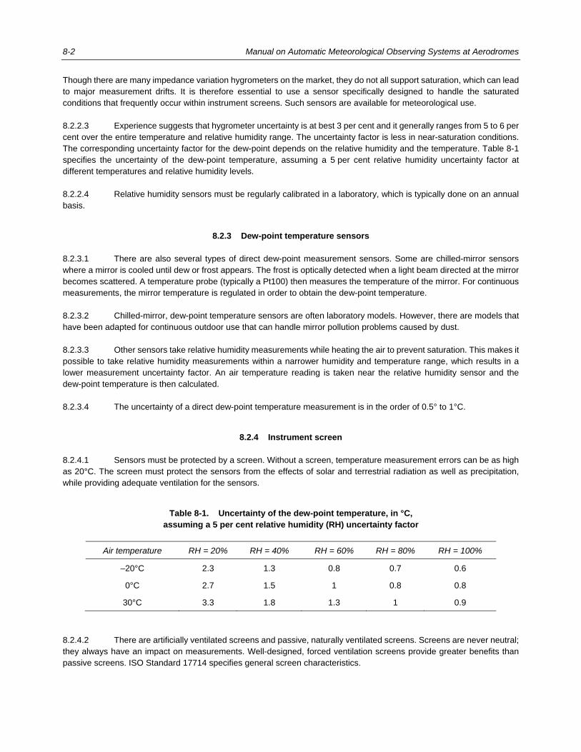
8-2 Manual on Automatic Meteorological Observing Systems at Aerodromes
Though there are many impedance variation hygrometers on the market, they do not all support saturation, which can lead to major measurement drifts. It is therefore essential to use a sensor specifically designed to handle the saturated conditions that frequently occur within instrument screens. Such sensors are available for meteorological use. 8.2.2.3 Experience suggests that hygrometer uncertainty is at best 3 per cent and it generally ranges from 5 to 6 per cent over the entire temperature and relative humidity range. The uncertainty factor is less in near-saturation conditions. The corresponding uncertainty factor for the dew-point depends on the relative humidity and the temperature. Table 8-1 specifies the uncertainty of the dew-point temperature, assuming a 5 per cent relative humidity uncertainty factor at different temperatures and relative humidity levels. 8.2.2.4 Relative humidity sensors must be regularly calibrated in a laboratory, which is typically done on an annual basis.
8.2.3 Dew-point temperature sensors 8.2.3.1 There are also several types of direct dew-point measurement sensors. Some are chilled-mirror sensors where a mirror is cooled until dew or frost appears. The frost is optically detected when a light beam directed at the mirror becomes scattered. A temperature probe (typically a Pt100) then measures the temperature of the mirror. For continuous measurements, the mirror temperature is regulated in order to obtain the dew-point temperature. 8.2.3.2 Chilled-mirror, dew-point temperature sensors are often laboratory models. However, there are models that have been adapted for continuous outdoor use that can handle mirror pollution problems caused by dust. 8.2.3.3 Other sensors take relative humidity measurements while heating the air to prevent saturation. This makes it possible to take relative humidity measurements within a narrower humidity and temperature range, which results in a lower measurement uncertainty factor. An air temperature reading is taken near the relative humidity sensor and the dew-point temperature is then calculated. 8.2.3.4 The uncertainty of a direct dew-point temperature measurement is in the order of 0.5° to 1°C.
8.2.4 Instrument screen 8.2.4.1 Sensors must be protected by a screen. Without a screen, temperature measurement errors can be as high as 20°C. The screen must protect the sensors from the effects of solar and terrestrial radiation as well as precipitation, while providing adequate ventilation for the sensors.
Table 8-1. Uncertainty of the dew-point temperature, in °C, assuming a 5 per cent relative humidity (RH) uncertainty factor
Air temperature RH = 20% RH = 40% RH = 60% RH = 80% RH = 100%
–20°C 2.3 1.3 0.8 0.7 0.6 0°C 2.7 1.5 1 0.8 0.8 30°C 3.3 1.8 1.3 1 0.9
8.2.4.2 There are artificially ventilated screens and passive, naturally ventilated screens. Screens are never neutral; they always have an impact on measurements. Well-designed, forced ventilation screens provide greater benefits than passive screens. ISO Standard 17714 specifies general screen characteristics.
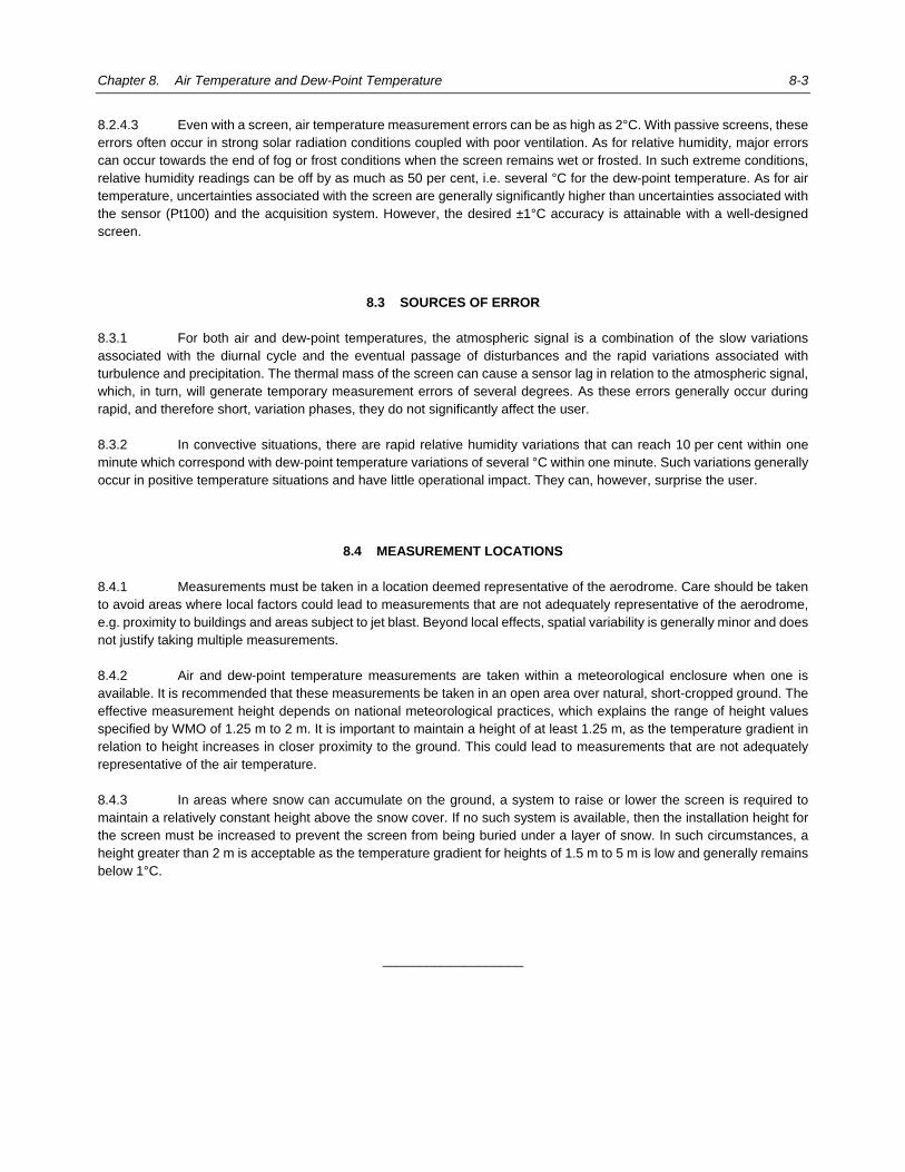
Chapter 8. Air Temperature and Dew-Point Temperature 8-3
8.2.4.3 Even with a screen, air temperature measurement errors can be as high as 2°C. With passive screens, these errors often occur in strong solar radiation conditions coupled with poor ventilation. As for relative humidity, major errors can occur towards the end of fog or frost conditions when the screen remains wet or frosted. In such extreme conditions, relative humidity readings can be off by as much as 50 per cent, i.e. several °C for the dew-point temperature. As for air temperature, uncertainties associated with the screen are generally significantly higher than uncertainties associated with the sensor (Pt100) and the acquisition system. However, the desired ±1°C accuracy is attainable with a well-designed screen.
8.3 SOURCES OF ERROR 8.3.1 For both air and dew-point temperatures, the atmospheric signal is a combination of the slow variations associated with the diurnal cycle and the eventual passage of disturbances and the rapid variations associated with turbulence and precipitation. The thermal mass of the screen can cause a sensor lag in relation to the atmospheric signal, which, in turn, will generate temporary measurement errors of several degrees. As these errors generally occur during rapid, and therefore short, variation phases, they do not significantly affect the user. 8.3.2 In convective situations, there are rapid relative humidity variations that can reach 10 per cent within one minute which correspond with dew-point temperature variations of several °C within one minute. Such variations generally occur in positive temperature situations and have little operational impact. They can, however, surprise the user.
8.4 MEASUREMENT LOCATIONS 8.4.1 Measurements must be taken in a location deemed representative of the aerodrome. Care should be taken to avoid areas where local factors could lead to measurements that are not adequately representative of the aerodrome, e.g. proximity to buildings and areas subject to jet blast. Beyond local effects, spatial variability is generally minor and does not justify taking multiple measurements. 8.4.2 Air and dew-point temperature measurements are taken within a meteorological enclosure when one is available. It is recommended that these measurements be taken in an open area over natural, short-cropped ground. The effective measurement height depends on national meteorological practices, which explains the range of height values specified by WMO of 1.25 m to 2 m. It is important to maintain a height of at least 1.25 m, as the temperature gradient in relation to height increases in closer proximity to the ground. This could lead to measurements that are not adequately representative of the air temperature. 8.4.3 In areas where snow can accumulate on the ground, a system to raise or lower the screen is required to maintain a relatively constant height above the snow cover. If no such system is available, then the installation height for the screen must be increased to prevent the screen from being buried under a layer of snow. In such circumstances, a height greater than 2 m is acceptable as the temperature gradient for heights of 1.5 m to 5 m is low and generally remains below 1°C.
___________________


9-1
Chapter 9
PRESSURE
9.1 INTRODUCTION 9.1.1 Pressure is measured at the altitude of the barometer installation. The value measured by the barometer is used to calculate QNH and QFE. 9.1.2 QNH is the pressure reduced to mean sea level (MSL), using the ICAO standard profile of the atmosphere (Manual of the ICAO Standard Atmosphere (extended to 80 kilometres (262 500 feet)) (Doc 7488) refers). QNH gives a normalized value of pressure, independent of the altitude of measurement. Altimeters using the same standard profile can deduce the aircraft altitude above a given point, knowing the QNH of this point. When set to a QNH altimeter setting, a pressure-type altimeter will indicate altitude above sea level and the official aerodrome altitude when landed. 9.1.3 QFE is the pressure reduced to an official aerodrome altitude, using the most appropriate profile of the atmosphere, thus taking in account, if necessary, the air temperature at the aerodrome. When set to a QFE altimeter setting, an altimeter will indicate height above the QFE reference level, and 0 when landed. The reference level for the computation of QFE should be the (official) aerodrome elevation. For non-precision approach runways with thresholds of 2 m (7 ft) or more below, or above, the aerodrome elevation, and for precision approach runways, additional QFEs should refer to the relevant threshold elevation.
9.2 ALGORITHMS 9.2.1 The pressure measured by the barometer (referred to as “Pbar”) must be expressed with a resolution equal to or lower than 0.1 hPa. Computation of QNH and QFE values must be done with a resolution equal to or lower than 0.1 hPa. Final and operational values of QNH and QFE are rounded down to the nearest whole hectopascal. 9.2.2 To determine QNH, QFE has to be calculated first, no matter whether it is reported or not, taking into account the altitude differences between the official level of the aerodrome and the effective altitude of the barometer. This calculation can use Doc 7488, using the effective air temperature at the time of calculation. For small height differences, a fixed value for the air temperature (15°C) can be used. Table 9-1 shows dp = QFE – Pbar for a difference of –10 m between the official height of the aerodrome (Href) and the height of the barometer (Hz), for several values of the air temperature. For realistic values of Href – Hz, the difference dP is proportional to the difference Href – Hz. It can be seen that the effect of a temperature difference of 30°C relative to +15°C is about 0.12 hPa. For small values of Href – Hz (< 10 m), the effective air temperature can be neglected for the calculation of QFE. For higher values, use of the effective air temperature is recommended.
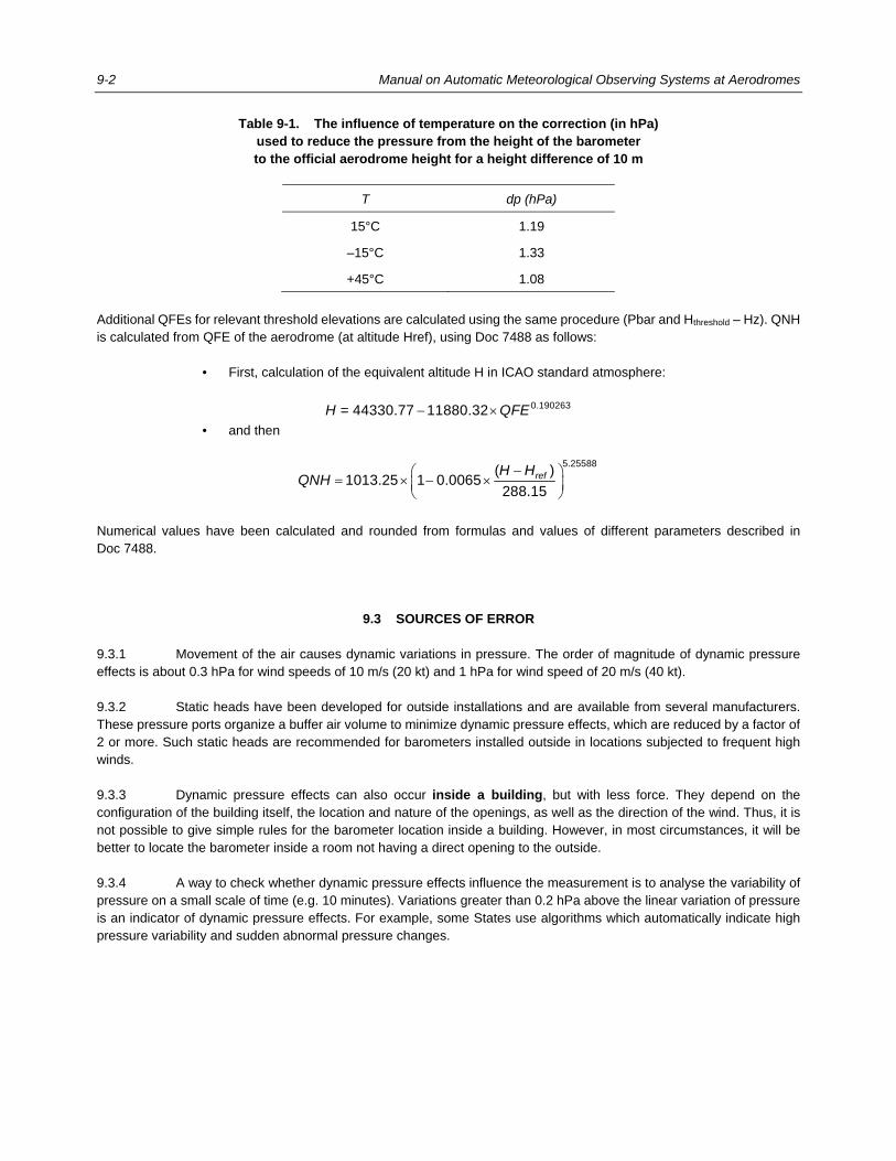
9-2 Manual on Automatic Meteorological Observing Systems at Aerodromes
Table 9-1. The influence of temperature on the correction (in hPa) used to reduce the pressure from the height of the barometer to the official aerodrome height for a height difference of 10 m
T dp (hPa)
15°C 1.19
–15°C 1.33
+45°C 1.08
Additional QFEs for relevant threshold elevations are calculated using the same procedure (Pbar and Hthreshold – Hz). QNH is calculated from QFE of the aerodrome (at altitude Href), using Doc 7488 as follows: • First, calculation of the equivalent altitude H in ICAO standard atmosphere:
− × 0.19026344330.77 11880.32H = QFE • and then
−⎛ ⎞= × − ×⎜ ⎟⎝ ⎠
refH HQNH
5.25588( )1013.25 1 0.0065
288.15
Numerical values have been calculated and rounded from formulas and values of different parameters described in Doc 7488.
9.3 SOURCES OF ERROR 9.3.1 Movement of the air causes dynamic variations in pressure. The order of magnitude of dynamic pressure effects is about 0.3 hPa for wind speeds of 10 m/s (20 kt) and 1 hPa for wind speed of 20 m/s (40 kt). 9.3.2 Static heads have been developed for outside installations and are available from several manufacturers. These pressure ports organize a buffer air volume to minimize dynamic pressure effects, which are reduced by a factor of 2 or more. Such static heads are recommended for barometers installed outside in locations subjected to frequent high winds. 9.3.3 Dynamic pressure effects can also occur inside a building, but with less force. They depend on the configuration of the building itself, the location and nature of the openings, as well as the direction of the wind. Thus, it is not possible to give simple rules for the barometer location inside a building. However, in most circumstances, it will be better to locate the barometer inside a room not having a direct opening to the outside. 9.3.4 A way to check whether dynamic pressure effects influence the measurement is to analyse the variability of pressure on a small scale of time (e.g. 10 minutes). Variations greater than 0.2 hPa above the linear variation of pressure is an indicator of dynamic pressure effects. For example, some States use algorithms which automatically indicate high pressure variability and sudden abnormal pressure changes.
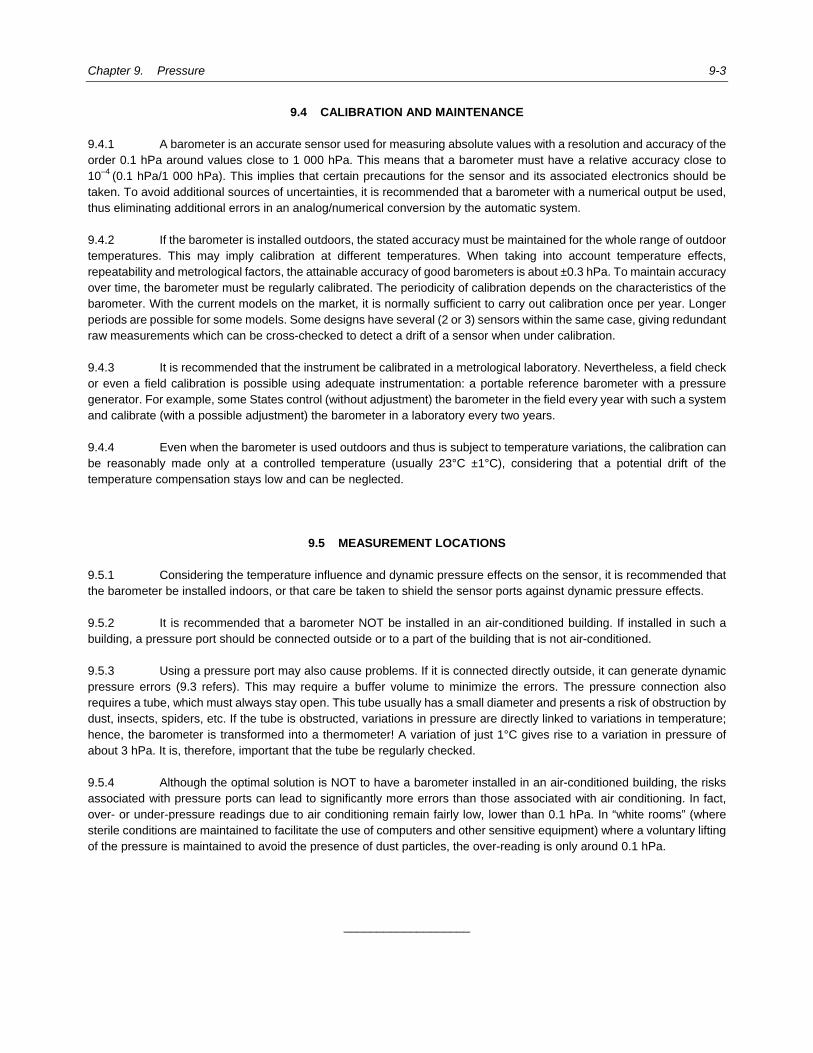
Chapter 9. Pressure 9-3
9.4 CALIBRATION AND MAINTENANCE 9.4.1 A barometer is an accurate sensor used for measuring absolute values with a resolution and accuracy of the order 0.1 hPa around values close to 1 000 hPa. This means that a barometer must have a relative accuracy close to 10–4 (0.1 hPa/1 000 hPa). This implies that certain precautions for the sensor and its associated electronics should be taken. To avoid additional sources of uncertainties, it is recommended that a barometer with a numerical output be used, thus eliminating additional errors in an analog/numerical conversion by the automatic system. 9.4.2 If the barometer is installed outdoors, the stated accuracy must be maintained for the whole range of outdoor temperatures. This may imply calibration at different temperatures. When taking into account temperature effects, repeatability and metrological factors, the attainable accuracy of good barometers is about ±0.3 hPa. To maintain accuracy over time, the barometer must be regularly calibrated. The periodicity of calibration depends on the characteristics of the barometer. With the current models on the market, it is normally sufficient to carry out calibration once per year. Longer periods are possible for some models. Some designs have several (2 or 3) sensors within the same case, giving redundant raw measurements which can be cross-checked to detect a drift of a sensor when under calibration. 9.4.3 It is recommended that the instrument be calibrated in a metrological laboratory. Nevertheless, a field check or even a field calibration is possible using adequate instrumentation: a portable reference barometer with a pressure generator. For example, some States control (without adjustment) the barometer in the field every year with such a system and calibrate (with a possible adjustment) the barometer in a laboratory every two years. 9.4.4 Even when the barometer is used outdoors and thus is subject to temperature variations, the calibration can be reasonably made only at a controlled temperature (usually 23°C ±1°C), considering that a potential drift of the temperature compensation stays low and can be neglected.
9.5 MEASUREMENT LOCATIONS 9.5.1 Considering the temperature influence and dynamic pressure effects on the sensor, it is recommended that the barometer be installed indoors, or that care be taken to shield the sensor ports against dynamic pressure effects. 9.5.2 It is recommended that a barometer NOT be installed in an air-conditioned building. If installed in such a building, a pressure port should be connected outside or to a part of the building that is not air-conditioned. 9.5.3 Using a pressure port may also cause problems. If it is connected directly outside, it can generate dynamic pressure errors (9.3 refers). This may require a buffer volume to minimize the errors. The pressure connection also requires a tube, which must always stay open. This tube usually has a small diameter and presents a risk of obstruction by dust, insects, spiders, etc. If the tube is obstructed, variations in pressure are directly linked to variations in temperature; hence, the barometer is transformed into a thermometer! A variation of just 1°C gives rise to a variation in pressure of about 3 hPa. It is, therefore, important that the tube be regularly checked. 9.5.4 Although the optimal solution is NOT to have a barometer installed in an air-conditioned building, the risks associated with pressure ports can lead to significantly more errors than those associated with air conditioning. In fact, over- or under-pressure readings due to air conditioning remain fairly low, lower than 0.1 hPa. In “white rooms” (where sterile conditions are maintained to facilitate the use of computers and other sensitive equipment) where a voluntary lifting of the pressure is maintained to avoid the presence of dust particles, the over-reading is only around 0.1 hPa.
___________________

10-1
Chapter 10
SUPPLEMENTARY INFORMATION
10.1 Annex 3 recommends adding the following information to local reports and/or METAR/SPECI messages: — recent weather (all reports);
— significant meteorological conditions in approach zones and climb-out zones, along with their location (local routine and special reports);
— wind shear (all reports); and
— state of the runway, sea surface temperature and state of the sea (METAR/SPECI subject to RAN agreement).
10.2 With an automatic system, supplementary information can be added only if the system is capable of detecting it.
10.3 An automatic system that provides present weather can also provide information on recent weather observed at the aerodrome since the last report or during the last hour. Among the recent weather phenomena, many can be reported by an automatic system, especially those concerning precipitation, i.e. recent rain (RERA), recent snow (RESN), recent drizzle (REDZ), recent heavy shower of rain (RESHRA), recent heavy snow (RESHSN) and possibly freezing precipitation (i.e. recent freezing drizzle (REFZDZ) and recent freezing rain (REFZRA)) and recent thunderstorms (RETS). The methods, characteristics and limitations of the automatic observation of present weather and applicable to recent weather are described in Chapter 6.
10.4 Information on most of the significant meteorological conditions (i.e. cumulonimbus clouds, thunderstorm, moderate or severe turbulence, wind shear, hail, severe squall line, moderate or severe icing, freezing precipitation, severe mountain waves, duststorm or sandstorm, blowing snow and funnel cloud (tornado or water spout)) required for inclusion in local reports, accompanied by an indication of the location of the phenomena concerned, cannot currently be reported automatically. However, remote sensing technology could be used in the future for this purpose.
10.5 Concerning the detection of wind shear, some airports are equipped with ground-based, wind shear remote-sensing or detection equipment (wind profiler or Doppler radar). In this case, information on significant wind shear can be automatically included in local reports and METAR/SPECI. There are also ground-based systems that detect wind shear based on multiple wind sensors located in an array (usually 12 to 16) at the aerodrome. These systems require that the site be surveyed beforehand. They produce warnings and provide digital or graphical information. They are usually installed at large airports and are not entirely automated. Nevertheless, they are a potential source for detection and automatic coding of wind shear as supplementary information for inclusion in local reports and METAR/SPECI.
10.6 Sea surface temperature and state of the sea can be detected automatically and included in METAR/SPECI when an automatic system is installed on an aeronautical platform at sea (designed for helicopters). The state of the sea is

10-2 Manual on Automatic Meteorological Observing Systems at Aerodromes
related to the wave height and can be automatically reported using swell gauges (i.e. instruments that measure wave height and wave periods). 10.7 The state of the runway is a non-meteorological parameter and is therefore not addressed in this manual.
___________________

11-1
Chapter 11
INTEGRATED MEASUREMENT SYSTEMS
11.1 CATEGORIES OF INTEGRATED MEASUREMENT SYSTEMS 11.1.1 Measurement systems can vary in complexity from simple systems composed of sensors and dedicated displays to systems that manage several runways or that are capable of automatically coding METAR/SPECI and local reports. 11.1.2 Displays are sometimes directly linked to sensors, especially when dealing with wind or pressure values. The simplest measurement systems can consist of wind, pressure, air temperature and humidity measurements. Some systems can locally calculate the required parameters (e.g. mean wind speed over 2 minutes and maximum and minimum values, QNH and QFE, and dew-point temperature). Thus, simple systems consisting of a sensor and its dedicated displays can be enough for local information, without requiring a central processing unit. These systems alone, however, cannot provide visibility and/or cloud information. They may be considered adequate for small aerodromes, where the ATS unit provides the pilot with information; however, they cannot automatically code METAR/SPECI. 11.1.3 Caution is necessary when installing such systems. In fact, using a minimal system sometimes leads to neglecting the instrument siting rules (particularly for wind) or the quality of sensors and their calibration. Mechanical barometers with needle gauges are sometimes used, but their metrological performance is much lower than recommended. Nevertheless, atmospheric pressure is particularly important for small aerodromes that do not have instrument landing systems (ILS). It is also common to see wind measurements taken directly from the roof of the control tower in conditions generating significant measurement errors. 11.1.4 The integrated systems have a central computer that combines all measurements, performs the necessary calculations and disseminates the information. The local dissemination of parameters is then done on the same line or terminal, which gathers all required information and displays it where it is needed. With such systems, there is no need to have dedicated displays for each sensor, unless stipulated by local agreements regarding the visual comfort or installation of fail-safe visual imagery systems. When specific displays are used, they are often associated with wind measurements and sometimes with pressure values (QNH/QFE). 11.1.5 The display of local information is therefore very often centralized on the same terminal. Two main possibilities exist: a) The terminal can be part of the meteorological measurement system. In this case, an image is
generated by the central computer, on an alphanumeric console or sometimes on a graphic console, which may include an outline chart of the aerodrome.
b) The display is not part of the meteorological measurement system, which regularly disseminates local
reports to an outside display unit. For example, the unit can be one of the specific computers of the aerodrome that can possibly display other useful information, besides meteorological information, to the ATS unit and other users.
11.1.6 At present, in partly automatic systems, measurements of wind, pressure, and air and dew-point temperature are always taken automatically. It is also possible to have one or more visibility measurement sensors, one or more ceilometers, or one or more sensors for RVR. A computer makes it possible to monitor measurements and complement

11-2 Manual on Automatic Meteorological Observing Systems at Aerodromes
them with manual input of cloud amount, type of clouds and present weather and supplementary information. With these complementary human observations, the computer does METAR/SPECI coding and formats local reports. 11.1.7 In fully automatic systems, METAR/SPECI coding is automatic and messages contain the word “AUTO”. Local reports are also coded automatically. At present, automatic systems cannot provide all the information required by Annex 3, so the coding remains partial. Not all automatic systems offer the same possibilities, which depend on the instruments and algorithms used. It is therefore necessary to inform the user, in the State’s Aeronautical Information Publication (AIP) (in accordance with the provisions of the Aeronautical Information Services Manual (Doc 8126)), about the capabilities and limitations of the systems in use. 11.1.8 The simplest systems measure wind, pressure, air and dew-point temperature. Such systems can provide useful information for small aerodromes, but their inherent limitations preclude a valid automatic coding of METAR/SPECI. 11.1.9 More advanced automatic systems also use a scatter meter for visibility, a ceilometer for cloud height base and for estimating cloud amount, and a sensor (or group of sensors) for present weather. This means they can provide information on visibility, clouds and present weather, but they have their limitations (e.g. visibility measured from a single point, multiple cloud layers indicated by one ceilometer and the detection of different types of present weather). Furthermore, the presence of CB or TCU clouds cannot be detected. However, such systems are designed to code METAR/SPECI AUTO and local reports. They are used for small aerodromes, and sometimes in conjunction with a human observer, during specified times. 11.1.10 More complete automatic systems can use multiple sensors for visibility, sometimes several ceilometers for clouds, complementary sensors for present weather (e.g. local flash detectors or information from a lightning measurement network), and information from a weather radar to detect the presence of convective clouds. RVR calculations can also be made. Such systems come closer to meeting the requirements laid out in Annex 3. The capabilities of complete systems depend on the sensors and algorithms used. Progress in this area may be expected in the coming years. 11.1.11 In any case, whatever the capabilities and limitations of a system, it is important to recall that “…, the specific value of any of the elements given in a report shall be understood by the recipient to be the best approximation to the actual conditions at the time of observation” (Annex 3, 4.1.9 refers). 11.1.12 It is true that, in some areas, an automatic system falls short of a human observer. However, there is often more documentation on the limitations of an automatic system than the limitations of a system that uses a human observer, which is sometimes, by definition, considered perfect — but that is not always the case. Visibility is an example: an observer located in a foggy area cannot identify the conditions at the runway threshold. More importantly, the information from an automatic system is sometimes more objective, since it is more clearly defined and consistent than information from a human observer. 11.1.13 The performance of an automatic system cannot be judged by comparing it directly to that of a human observer, but rather by the overall quality of the service provided to the aeronautical user. An automatic system and a human observer do not use the same observation methods. For example, analysing signals from a ceilometer aimed vertically to determine cloud layers sometimes gives wrong results. This can also be the case, but for different reasons, with night-time human observations. 11.1.14 Diagrams of various systems are given in Figures 11-1, 11-2 and 11-3.
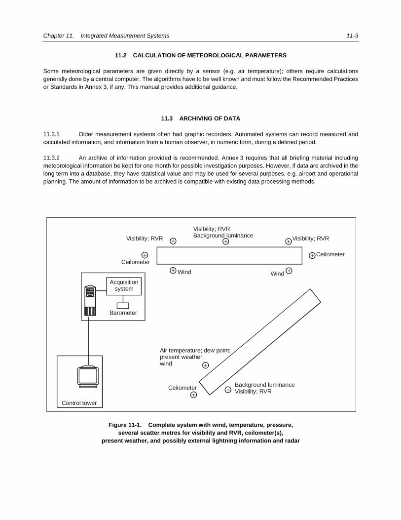
Chapter 11. Integrated Measurement Systems 11-3
11.2 CALCULATION OF METEOROLOGICAL PARAMETERS Some meteorological parameters are given directly by a sensor (e.g. air temperature); others require calculations generally done by a central computer. The algorithms have to be well known and must follow the Recommended Practices or Standards in Annex 3, if any. This manual provides additional guidance.
11.3 ARCHIVING OF DATA 11.3.1 Older measurement systems often had graphic recorders. Automated systems can record measured and calculated information, and information from a human observer, in numeric form, during a defined period. 11.3.2 An archive of information provided is recommended. Annex 3 requires that all briefing material including meteorological information be kept for one month for possible investigation purposes. However, if data are archived in the long term into a database, they have statistical value and may be used for several purposes, e.g. airport and operational planning. The amount of information to be archived is compatible with existing data processing methods.
Figure 11-1. Complete system with wind, temperature, pressure,
several scatter metres for visibility and RVR, ceilometer(s), present weather, and possibly external lightning information and radar
Control tower
Background luminanceVisibility; RVR+
+
+
+
+
++
+
+
+
Barometer
Acquisitionsystem
Ceilometer
Air temperature; dew point;present weather;wind
Wind Wind
Ceilometer
Visibility; RVRVisibility; RVRBackground luminanceVisibility; RVR
Ceilometer

11-4 Manual on Automatic Meteorological Observing Systems at Aerodromes
Figure 11-2. ASOS-type automatic system, with wind, temperature,
pressure, scatter metre, ceilometer and present weather
Figure 11-3. Simple system with pressure, temperature,
wind sensors and dedicated displays
Temperature
Wind
QNH
QFEBarometer
Pressure
Control tower
T
DP
Control tower
Barometer
Acquisitionsystem
Air temperature Wind
Present weather
Scatter meter(Visibility)(RVR)
Ceilometer

Chapter 11. Integrated Measurement Systems 11-5
11.4 DATA ACQUISITION TECHNIQUES 11.4.1 To provide a representative sample, meteorological sensors are sometimes spread out over the aerodrome. The information must then be transmitted to one of the central computers of the system. 11.4.2 In order to avoid data loss and corruption, analog signals from sensors should not be transported over a long distance. It is better to convert analog signals into digital signals at the sensor site or to have an acquisition system in a meteorological enclosure close to the sensors. 11.4.3 Many sensors, particularly complex sensors such as scatter meters, ceilometers or present weather sensors which have to process raw signals, now provide digital output. 11.4.4 The central computer is therefore fed by one or more “digital” lines, such as telephone lines and modems, telephone lines and RS485 current loops, fibre optics and radio transmissions. The methods used must also take into account protection against electromagnetic discharge. The techniques used should be robust and must often adapt to the transmission lines available at the aerodrome. Note that the cost of installing a cable can be a lot higher than the cost of the sensor itself.
11.5 PERFORMANCE CHECK AND MAINTENANCE 11.5.1 It is normal practice to check the operation of instruments, sensors, computers and data systems at regular intervals and to carry out proper maintenance. The maintenance constraints and periodicity depend on the type of instruments used, local conditions and the manufacturer’s recommendations (Chapters 3 to 9 refer). 11.5.2 There should be preventive and corrective maintenance plans for each sensor and for the entire system. All elements of an automatic system can malfunction or break down. Some sensors are currently capable of giving warnings of reduced performance before actually breaking down, e.g. battery voltage, contamination of optical surfaces, radiating power of a laser diode and comparison of redundant measurements. Having a central computer makes it possible to perform cross-checks between parameters to detect possible anomalies or drifts. If many sensors measuring the same type of parameter (meteorological optical range, for example) are installed, it is useful to statistically examine their variances. 11.5.3 Maintenance should be organized so that intervention time frames and the likelihood of successful repair can be predicted. Successful repair depends on the expertise of maintenance staff and on the availability and location of spare parts. Some sensors should be duplicated for back-up purposes, as should the actual data acquisition and processing system, particularly at large aerodromes. Duplication leads to greater safety and reduces the burden on maintenance staff and, therefore, could be a valid economical alternative.
11.6 FREQUENCY OF ISSUE 11.6.1 METAR must be issued every hour and sometimes every half-hour, according to regional procedures. 11.6.2 SPECI must be issued according to deterioration and improvement criteria defined in Annex 3 (Appendix 3, 2.3.2 refers). Automatic detection of SPECI conditions from measured information is possible. The experience with ASOS systems shows that automatic detection results in many more SPECIs (about three times more) than when the SPECI conditions are determined by a human observer. Human observers use their knowledge of the meteorological situation and analytical abilities to avoid the issuance of multiple SPECI. Despite the 10-minute time frame required to take an improvement into account, an automatic system generates more messages. An airport with multiple RVR equipment is likely to see RVR limits overstepped several times, for deteriorations and improvements, by the different sensors. A human observer, on the other hand, sorts the information mentally and thus limits the number of SPECI.

11-6 Manual on Automatic Meteorological Observing Systems at Aerodromes
11.6.3 The reporting frequency for local reports is the same as that for METAR. However, displays are required, for use by ATS units, for wind, RVR and pressure and are recommended for the height of cloud base, and air and dew-point temperatures. These displays depict parameters that are variable in time, such as wind, visibility and RVR, and, therefore, need to be updated frequently. A one-minute frequency is acceptable. Most parameters must represent a period of at least one minute. If they are calculated once per minute, which is often the case, it is not useful to issue the information more often. Certain parameters, such as wind, can be calculated using a greater frequency. An update rate greater than one minute is then possible, particularly if it is done on a channel specifically for wind (dedicated display). If the issuance is done on a single channel, with all the information, a one-minute period is a good compromise. A longer period must be avoided.
___________________

12-1
Chapter 12
REMOTE SENSING
12.1 INTRODUCTION 12.1.1 Annex 3 does not require the installation of remote sensing equipment for meteorological observations. Some systems, however, do offer interesting possibilities for aeronautical users, but the current method used to issue meteorological information, i.e. the use of local reports and METAR/SPECI, is an obstacle to getting the most out of the information they offer. The advantages of these reports are that they are simple, clearly defined and therefore recognized by aeronautical users. METAR/SPECI can also be disseminated on all telecommunications channels, even on the simplest, which is useful when the communication infrastructure is poor. However, some information is lost when data from remote sensing systems is reduced to a few characters in an alphanumeric message, but this process is sometimes necessary to access information easily. A typical example of this problem is the detection of convective cells using a radar from which information can be extracted to indicate the presence of CB or TCU clouds (see Chapter 7). A radar image prepared to show these major reflectivity zones, however, contains more detailed information on the extent of the zone, its movement and its severity. This could be useful for both the pilot and ATS unit, who could anticipate possible diversions. Such observation methods are sometimes used but are not currently standardized. 12.1.2 This chapter will describe the possibilities of certain remote sensing systems.
12.2 MEASUREMENT METHODS AND POTENTIALS
12.2.1 Radar images 12.2.1.1 The use of radar images to detect and locate CB and TCU clouds was discussed in Chapter 7. 12.2.1.2 A radar image (or a radar image composite) is not always perfect and can contain errors such as echoes from stationary objects or a bright band (liquid/solid transition). Therefore, a raw image must often be interpreted by a professional meteorologist and does not always meet aeronautical operational needs. Rather than using a raw image, it is more effective to extract or prepare a more user-friendly product. One State is experimenting with such a product which has four reflectivity thresholds and a smoothing of convective zones, with the possibility of superimposing lightning information. This product makes it possible for ATS units, through their knowledge of high reflectivity zones, to anticipate the possible deviation of aircraft, which often have their own on-board radar providing analogue information. This sort of image contains much more information than the simple presence or absence of CB or TCU clouds included in a METAR/SPECI. 12.2.1.3 Apart from detecting rainfall, radar with Doppler capability can also be used to detect microbursts and wind shear in the terminal area. Typically, such a radar is located at a height close to the aerodrome level so that it can scan the lowest few hundred metres for divergence or convergence wind patterns. It should also have an unobstructed view of the runway and its radar beam when pointing towards the runway. It should almost be parallel to the runway direction. The radar detects the radial winds to determine the wind shear conditions on the runway and the approach and departure corridors. With appropriate software, the wind shear information can be graphically displayed to indicate the location and intensity of wind shear. Alphanumeric alerting messages containing wind shear location and intensity information for

12-2 Manual on Automatic Meteorological Observing Systems at Aerodromes
specific runway corridors can also be generated for dissemination to the ATS units concerned and for inclusion in the local reports and METAR/SPECI as discussed in Chapter 10.
12.2.2 Lightning network 12.2.2.1 There are networks that detect lightning based on its electromagnetic signature (Chapter 6 refers). The most widely used technology detects cloud-ground lightning with a precision of location that depends on the density of the network and its topology, e.g. with sensors spaced at 200 km, the precision can reach 1 km. More localized cloud-ground and cloud-to-cloud lightning detection systems also exist. 12.2.2.2 This type of network is the best way of determining the electrical activity associated with thunderstorms and is a valuable complementary tool for meteorologists. It makes it possible to locate electrical activity in real time with excellent precision of location. Although this information makes it possible to report to an automatic system the presence of a thunderstorm at the airport or in its vicinity, the technical difficulty lies in transmitting the information in real time from the central computer of a lightning network to an automatic observation system at the airport. With the evolution of telecommunication offering more and more technical possibilities, developments using information from a lightning network to report present weather TS or VCTS and possibly the presence of CB clouds in local reports and METAR/SPECI are under way in many States (Chapters 6 and 7 refer).
12.2.3 Satellite images Satellite images using the infrared wavelengths allow the measurement of the temperature at the top of clouds and, combined with high radar reflectivities, the identification of thunderstorm cells and CB and TCU clouds, which have a large vertical extent and which therefore have cold cloud tops. Instruments that automatically identify thunderstorm cells have been developed in some countries and can be used, along with radar images, to identify CB and TCU.
12.2.4 Wind profilers 12.2.4.1 Wind profilers measure the vertical profile of wind and can be useful for sites subject to wind shear. 12.2.4.2 There are two types of wind profilers based on ultrasound (SODAR) and electromagnetic waves (UHF radar). An antenna system emits pulses in several vertical directions. Part of the signal emitted is backscattered by small inhomogeneities in the atmosphere (such as variations in the refractive index) to the antenna system which serves as a receiver. The time the signal takes to return determines the distance. The frequency of the signal shifts according to the radial movement of the atmospheric zone that backscattered the signal (Doppler effect). The combination of radial speeds in the different pulse directions (at least three) makes it possible to calculate the horizontal speed in different altitude bands. 12.2.4.3 These instruments can calculate high-frequency profiles, every 10 minutes for example, ensuring a follow-up in real time. Profiles can contain errors caused by parasitic signals; therefore, filtering algorithms are required. These algorithms mostly use the preceding profiles to monitor the temporal coherence of successive profiles. The output of such systems is typically a temporal succession of wind profiles represented as vectors. It is possible to set wind shear thresholds to extract a synthetic indication that can be used locally by the ATC and possibly included in local reports and METAR/SPECI as supplementary information.
12.2.5 Light detection and ranging (LIDAR) A LIDAR emits typically an invisible laser light pulse and analyses the return signal backscattered by the atmosphere in one or more directions, from which it can deduce the wind, the extinction coefficient and other parameters. A slant

Chapter 12. Remote Sensing 12-3
measurement from a distance would make it possible to measure the wind above the runway or in the approach zone. Unfortunately, the optical signal can be reduced by rain, clouds or fog, in which case the instrument is blinded and its usefulness diminished. Nevertheless, a LIDAR is useful in detecting wind shear in clear air conditions (e.g. wind shear induced by sea breezes, gust fronts ahead of thunderstorms, or topography). This type of instrument is expensive and, in the past, it has been used only for research; more recently, it has been deployed at some aerodromes for wind shear monitoring.
___________________


13-1
Chapter 13
QUALITY ASSURANCE
13.1 Annex 3 (Section 2.2) recommends a quality management system guaranteeing that the products and services meet the needs of aeronautical users. Note.— This requirement to establish and implement a properly organized quality system becomes a Standard from 15 November 2012. 13.2 Quality management should follow ISO 9000 version 2008 ensuring that products and services match user needs; these standards introduce the idea of continuous quality improvement. 13.3 In a system of quality management, the needs must be translated into realistic goals known to and accepted by the user. Products and services must be adapted to the goals, and there must be a way of measuring whether the goals have been achieved. Finally, faults must be corrected, bearing in mind the limits of the quality management system. 13.4 The general scheme is: a) know user requirements; b) identify the processes set up to respond to these requirements; c) define the goals of the various processes; d) have users accept these goals (or renegotiate); e) set up methods to achieve the goals; f) measure achievement of goals and set up appropriate indicators; g) follow up performance and identify and address anomalies; h) assess user satisfaction; i) take corrective and preventive action; and j) link the different operations with a view to continuous quality improvement (plan – do – check – act). 13.5 In the case of an automatic aerodrome observation system, the scheme is roughly as follows: a) know the requirements of aeronautical users. Annex 3 (Chapter 4 and Appendix 3) provides the basis
for meteorological observation; b) identify and document the processes of production, management and support in relation to aeronautical
meteorological observation; c) define the goals: capacities of an automatic system, associated performances, reliability sought,
acceptable and unacceptable time frames for repair services;

13-2 Manual on Automatic Meteorological Observing Systems at Aerodromes
d) have users accept goals (or renegotiate) and file, if required, an official notification of difference. A lack of resources or personnel (in the case of human observation) might mean that systems and/or observation methods are installed that do not satisfy all the ICAO Standards and Recommended Practices. Quality must depend on a clear definition of the possibilities and limits of the system and of the associated services;
e) make sure that the goals are achieved, i.e. define human maintenance, spare parts, preventive
maintenance, etc. The rules and solutions are many; what is essential is that they be defined and assessed. This is particularly important for automatic systems, which can easily be “forgotten” precisely because they are automatic. This applies especially to simple systems at small aerodromes where the financial means for observation might be reduced;
f) define the calibration and maintenance frequency; g) measure achievement of goals and set up appropriate indicators; h) follow up performance and identify and address anomalies; i) measure user satisfaction and actions for quality improvement; j) assess user satisfaction regarding the service of automatic systems, both in terms of local reports and
METAR/SPECI; and k) take corrective and preventive action. This means improving the system over its lifetime in order to
increase capacity and decrease the limitations. This is particularly important for automatic observation systems, which cannot yet fulfil all the requirements in Annex 3.
13.6 Quality goals and the processes for meeting them should be taken into account also in the procurement of an automatic aerodrome observing system. Specifications of the system should be written to reflect the requirements of quality assurance. 13.7 Before a new system is taken into use, the organization responsible should ascertain that the products supplied meet its specifications. Examples of the verification of conformance to specifications are given below: a) own testing; b) inspection at a factory acceptance test; c) reliable evidence provided by the supplier, e.g.: — third-party test reports or certificates issued by a competent authority, based on documented
testing and applying uniform criteria; — other documentation such as credible tests carried out and documented by the supplier. Note 1.― Performance of some meteorological sensors can be difficult to verify due to the lack of standardized definitions for accuracy. Particular care should be taken in specifying the performance of these instruments, e.g. present weather and cloud sensors. Methods of verification should be specified in conjunction with accuracy goals, as they are interdependent. Note 2.― Guidance on specifying meteorological instruments is given in Appendix B.
___________________

App A-1
Appendix A
ALGORITHMS
The algorithms that follow are intended to be used as examples only. It should be noted that they do not provide an exhaustive list and that it is likely that some algorithms, particularly those involving present weather, may not be suitable in some parts of the world owing to climatological variations.
Wind direction (1) Wind direction is separated into two groups: one group for those in the eastern hemisphere (i.e. 0° < direction <= 180°) with e number of data points and the other group for the western hemisphere (i.e. 180° < direction <= 360°) with w number of data points. The mean value for the eastern hemisphere, DE , and the mean value for the western hemisphere, DW, are calculated as: DE = (sum of all directions in the eastern hemisphere)/e DW = (sum of all directions in the western hemisphere)/w When the difference is less than or equal to 180° (i.e. (DW - DE) <= 180°), the wind direction is clustered more generally towards the southern hemisphere. The mean direction is calculated as: mean direction = [ DW x w + DE x e ] / [ w + e ] When the difference is greater than 180° (i.e. (DW − DE) > 180°), the wind direction is clustered more generally towards the northern hemisphere. Then the mean direction is calculated as: mean direction = [ (DW − 360°) x w + DE x e ] / [ w + e ] If this result is less than or equal to 0°, then add 360° to the mean direction.
Marked wind discontinuity (2) This may be used as follows: a) to take into account a change in direction of 30°, the instantaneous directions should not be used
directly, since rapid changes reach and often top 30°, without an overall change in wind direction; b) a marked discontinuity must be maintained for at least 2 minutes, so the mean wind must be used over
2 minutes (speed and direction); c) to calculate ff2 and DD2 (the mean speed and direction values over the last 2 minutes); d) to calculate ff8 and DD8 (the mean speed and direction values over 8 minutes), calculated 2 minutes
before (i.e. it does not take into account the last 2 minutes). To limit calculations, it is also possible to use

App A-2 Manual on Automatic Meteorological Observing Systems at Aerodromes
the mean value over 10 minutes, calculated 2 minutes before. The result will not differ much and the mean value over 10 minutes is usually calculated regularly;
e) to compare DD2 with DD8. If both mean directions differ by more than 30° and the mean wind before or
after (ff2 or ff8) is above 5 m/s (10 kt), there is a marked discontinuity 2 minutes ago; f) to compare ff2 with ff8. If the absolute difference is above 5 m/s (10 kt), there is a marked discontinuity; and g) if a marked discontinuity is detected, to note the moment it occurs in order to calculate the successive
mean value. When the marked discontinuity is detected, the last value calculated over 2 minutes must be used for the mean value. For the following minute, the parameters will be calculated over a period of 3, then 4, minutes until the normal 10-minute period is caught up with.
Marked wind discontinuity (3)
This may be used as follows: a) to take into account a change of direction of 30°, the instantaneous directions should not be used
directly since rapid changes reach and often exceed 30° without any overall change in the wind direction;
b) a marked discontinuity must be maintained for at least 2 minutes, so the mean wind must be used over
2 minutes (speed and direction); c) to calculate ff2 and DD2 (the mean speed and direction values over the last 2 minutes); d) to calculate ff8 and DD8 (the mean speed and direction values over 8 minutes), calculated 2 minutes
before (i.e. it does not take into account the last 2 minutes). To limit calculations, it is also possible to use the mean values over 10 minutes, calculated 2 minutes before. The result will not differ much and the mean value over 10 minutes is usually calculated regularly;
e) to compare DD2 with DD8. If both mean directions differ by more than 30° and the mean wind before or
after (ff2 or ff8) is above 5 m/s (10 kt), there is a marked discontinuity 2 minutes ago. However, if the 2-minute wind direction variation is greater than or equal to 60°, then discard the marked discontinuity and go to step c);
f) compare ff2 with ff8. If the absolute difference is above 5 m/s (10 kt), there is a marked discontinuity
2 minutes ago. However, if the 2-minute wind direction variation is greater than or equal to 60°, then discard the marked discontinuity and go to step c); and
g) if a marked discontinuity is detected, note the moment it occurs, in order to calculate the successive mean
values. When the marked discontinuity is detected, the last value calculated over 2 minutes must be used for the mean value. For the following minute, the parameters will be calculated over a period of 3, then 4 minutes until the normal 10-minute period is reached.
Detection and removal of artificial gusts (4) Every effort has to be made to site an anemometer in an aerodrome to avoid the effect of artificial gusts, e.g. from jet efflux or wake vortices. The use of the algorithm below to detect and remove artificial gusts is the last resort.

Appendix A. Algorithms App A-3
The essence of the algorithm is that it is possible to distinguish in real time between artificial and natural peak gusts. If a peak gust is identified as an artificial gust then the measured data is modified, taking into account previous measurements up to 10 minutes ago. Artificial gusts are recognized because of their extreme behavior and typical structure which deviate from natural wind speed fluctuations. Moreover, such gusts typically exceed values of the maximum allowable normalized wind speed. The value of this maximum depends on the terrain roughness or local roughness length and should be determined first before implementing this algorithm. Fine-tuning of the constants used is recommended to improve its performance. Detection of artificial gusts: a) Calculate a dimensionless parameter called normalized extreme wind un as follows: un = (umax – U)/ σu
where: umax = actual, i.e. instantaneous, measured wind gust (3-second average); U = 10-minute mean wind speed; and σu = standard deviation of this 10-minute wind speed (U and σu are calculated using the same wind
speed data). b) A wind gust is considered to be artificial if: un > 5. The threshold value of 5 is found by experiment and will depend only on the terrain roughness,
expressed by its roughness length z0 (the value given for open terrain, z0 = 0.03 m). Removal of artificial gusts: a) To reduce the risk of removing genuine gusts, the artificial gust removal algorithm will be applied only to
the following situation: U > 0.5 m/s, σu > 0.5 m/s and umax < 15 m/s. For low wind situations both U and σu may become zero, in which case un is not defined. For cases with
large gusts in excess of 15 m/s, no removal of gusts will be made to avoid risks. b) The reduced gust u is estimated as: u = U b σu + c where: b and c are constants. b is about 2.5 whereas c can range between 0 m/s and 0.5 m/s. They can be
fine-tuned by experiment. Note.― Because the algorithm should not be used outside the specified criteria, artificial gusts are
not modified (or corrected) under these circumstance (typically with low wind speeds where the impact of a wake vortex is significant). In these cases, with U and σu almost 0 m/s the system may provide the user with an identifier (flag) to indicate that an artificial gust is identified but not filtered out.
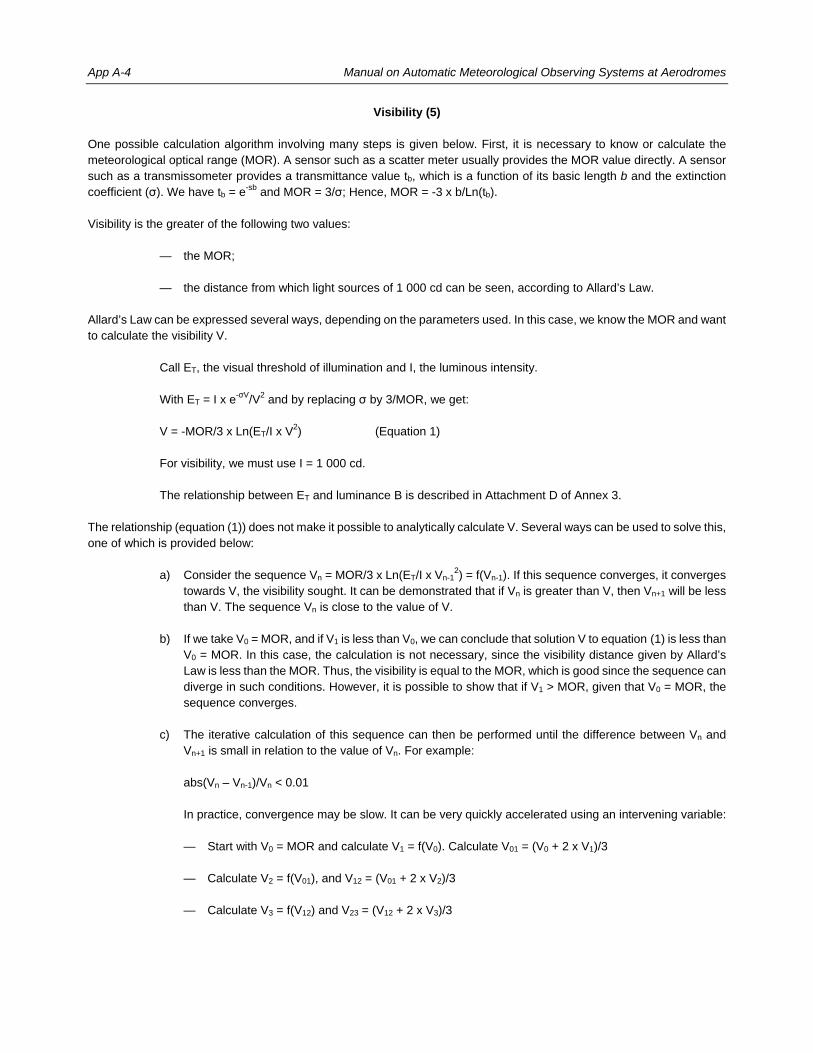
App A-4 Manual on Automatic Meteorological Observing Systems at Aerodromes
Visibility (5) One possible calculation algorithm involving many steps is given below. First, it is necessary to know or calculate the meteorological optical range (MOR). A sensor such as a scatter meter usually provides the MOR value directly. A sensor such as a transmissometer provides a transmittance value tb, which is a function of its basic length b and the extinction coefficient (σ). We have tb = e-sb and MOR = 3/σ; Hence, MOR = -3 x b/Ln(tb). Visibility is the greater of the following two values: — the MOR; — the distance from which light sources of 1 000 cd can be seen, according to Allard’s Law. Allard’s Law can be expressed several ways, depending on the parameters used. In this case, we know the MOR and want to calculate the visibility V. Call ET, the visual threshold of illumination and I, the luminous intensity. With ET = I x e-σV/V2 and by replacing σ by 3/MOR, we get: V = -MOR/3 x Ln(ET/I x V2) (Equation 1) For visibility, we must use I = 1 000 cd. The relationship between ET and luminance B is described in Attachment D of Annex 3. The relationship (equation (1)) does not make it possible to analytically calculate V. Several ways can be used to solve this, one of which is provided below: a) Consider the sequence Vn = MOR/3 x Ln(ET/I x Vn-1
2) = f(Vn-1). If this sequence converges, it converges towards V, the visibility sought. It can be demonstrated that if Vn is greater than V, then Vn+1 will be less than V. The sequence Vn is close to the value of V.
b) If we take V0 = MOR, and if V1 is less than V0, we can conclude that solution V to equation (1) is less than
V0 = MOR. In this case, the calculation is not necessary, since the visibility distance given by Allard’s Law is less than the MOR. Thus, the visibility is equal to the MOR, which is good since the sequence can diverge in such conditions. However, it is possible to show that if V1 > MOR, given that V0 = MOR, the sequence converges.
c) The iterative calculation of this sequence can then be performed until the difference between Vn and
Vn+1 is small in relation to the value of Vn. For example: abs(Vn – Vn-1)/Vn < 0.01 In practice, convergence may be slow. It can be very quickly accelerated using an intervening variable: — Start with V0 = MOR and calculate V1 = f(V0). Calculate V01 = (V0 + 2 x V1)/3 — Calculate V2 = f(V01), and V12 = (V01 + 2 x V2)/3 — Calculate V3 = f(V12) and V23 = (V12 + 2 x V3)/3
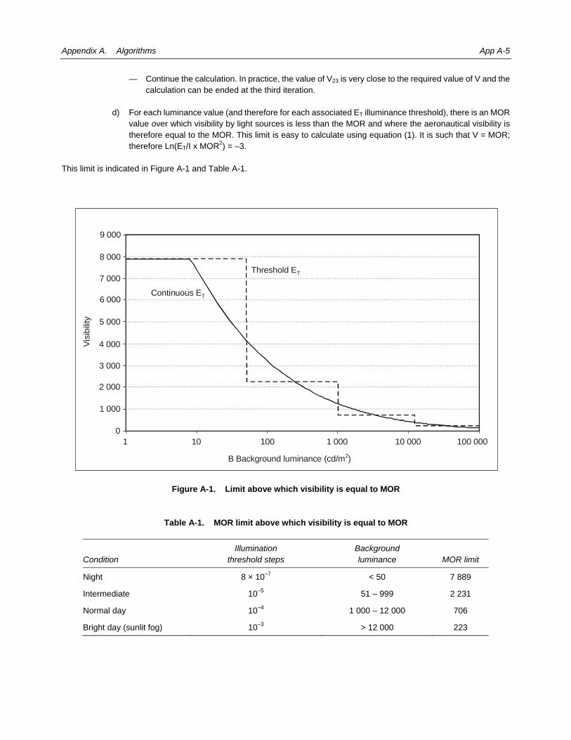
Appendix A. Algorithms App A-5
— Continue the calculation. In practice, the value of V23 is very close to the required value of V and the calculation can be ended at the third iteration.
d) For each luminance value (and therefore for each associated ET illuminance threshold), there is an MOR
value over which visibility by light sources is less than the MOR and where the aeronautical visibility is therefore equal to the MOR. This limit is easy to calculate using equation (1). It is such that V = MOR; therefore Ln(ET/I x MOR2) = –3.
This limit is indicated in Figure A-1 and Table A-1.
Figure A-1. Limit above which visibility is equal to MOR
Table A-1. MOR limit above which visibility is equal to MOR
Condition Illumination
threshold steps Background luminance MOR limit
Night 8 × 10⁻⁷ < 50 7 889
Intermediate 10–5 51 – 999 2 231
Normal day 10–4 1 000 – 12 000 706
Bright day (sunlit fog) 10–3 > 12 000 223
9 000
101 100 1 000 10 000 100 0000
1 000
2 000
3 000
4 000
5 000
6 000
7 000
8 000
Visi
bilit
y
Continuous ET
Threshold ET
B Background luminance (cd/m )2

App A-6 Manual on Automatic Meteorological Observing Systems at Aerodromes
Present weather detection (6) The following conditions normally lead to an absence of precipitation; therefore, an incorrect diagnostic from the sensor can be corrected. Tair, T+10, and T+50 refer to the standard screen temperature measurement and temperatures measured at 10 cm and 50 cm above the ground, respectively. — Difference Tair – T+10 > 3°C over a 20-minute period → no precipitation. — Difference T+50 – T+10 > 1.5 °C over a 20-minute period → no precipitation. — (T+50 > Tair + 2) and (T+10 > T+50 + 2) daytime → no precipitation. — No clouds detected above 4 500 m (15 000 ft) → no precipitation. — Visibility > 40 km for 5 minutes → no precipitation. — Relative humidity (RH) < 50 per cent → no precipitation. — RH diminishes or the difference between Tair and dew-point depression increases and visibility
increases → no precipitation. — Sudden diminution of difference between T+50 and T+10 (outside sunrise and sunset) → start of
precipitation or arrival or fog. — Isothermia (constant temperature) of T+50 or T+10 at 0°C (or temperature very close to 0°C, considering
uncertainty of measurement) → melting snow probable.
Present weather identification (7)
Example 1 — Cases of snow with a Tair > 4°C are very rare. — When Tair < –5°C, there is no longer any liquid precipitation. Note.— The above criteria are not always applicable, especially in cold climates where liquid precipitation can exist at significantly lower temperatures. — Cases of mixed rain and snow occur almost always with Tair in the interval [–1°C, 5°C]. — Isothermal (constant temperature) of T+50 or T+10 at 0°C (or temperature very close to 0°C, considering
uncertainty of measurement) → melting snow probable (and melting snow if a present weather sensor has diagnosed precipitation). Sometimes, hoar frost or freezing fog.
— Wet-bulb temperature, noted as Twb, presents a limit for rain and snow. Snow is not observed when Twb > 1.5°C. — Position in a Tair diagram, RH or a Twb diagram, RH (see Figure A-2). There are zones where some
varieties of hydrometeor are observed alone, and some zones where some varieties are not observed. Such diagrams alone are not enough to determine the type of hydrometeor, but they can help identify or correct the initial diagnostic by the sensor. For example, at a negative temperature with an RH less than
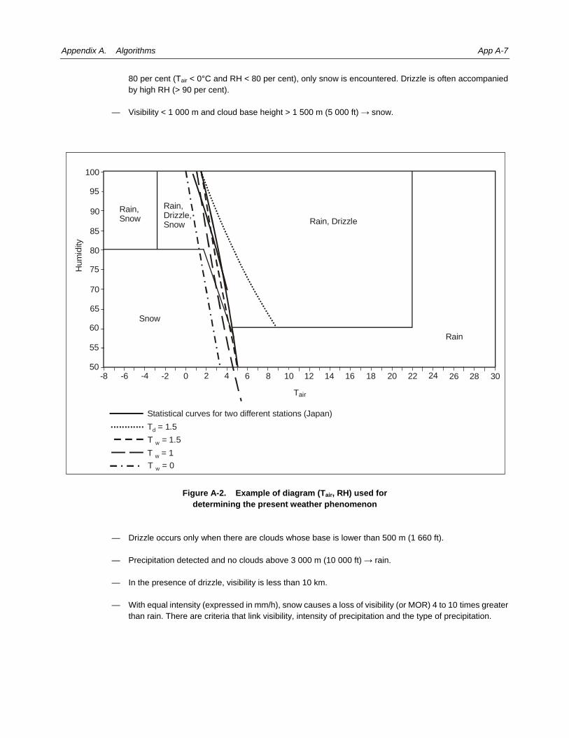
Appendix A. Algorithms App A-7
80 per cent (Tair < 0°C and RH < 80 per cent), only snow is encountered. Drizzle is often accompanied by high RH (> 90 per cent).
— Visibility < 1 000 m and cloud base height > 1 500 m (5 000 ft) → snow.
Figure A-2. Example of diagram (Tair, RH) used for
determining the present weather phenomenon — Drizzle occurs only when there are clouds whose base is lower than 500 m (1 660 ft). — Precipitation detected and no clouds above 3 000 m (10 000 ft) → rain. — In the presence of drizzle, visibility is less than 10 km. — With equal intensity (expressed in mm/h), snow causes a loss of visibility (or MOR) 4 to 10 times greater
than rain. There are criteria that link visibility, intensity of precipitation and the type of precipitation.
Statistical curves for two different stations (Japan)T = 1.5d
T = 1.5w
T w = 1T w = 0
Rain, DrizzleRain,Snow
Rain,Drizzle,Snow
Snow
-8 0 2-6 -4 -2 4 6 8 10 12 14 16 18 20 22 24 26 3028
100
95
90
85
80
75
70
65
Hum
idity
50
55
60Rain
Tair
App A-8 Manual on Automatic Meteorological Observing Systems at Aerodromes
Example 2 Firstly, a correction of the precipitation type is applied when applicable. This correction includes the verification of whether the liquid precipitation is freezing or not by using the wet-bulb temperature (Tw) derived from the operational ambient air temperature sensor (Ta). In addition, sensor reports of snow/grains and ice pellets are subjected to some tests and set to unknown precipitation or a mixture of snow and rain depending on the wet-bulb temperature and the precipitation intensity. The full set of corrections applied when all required information is available is: a) If Tw = 0°C, change RA and mixture RADZ into FZRA and DZ into FZDZ; b) If Tw > 0°C, change FZRA into RA and FZDZ into DZ; c) If Ta > –10°C, change IC into UP; d) If Ta > 7°C, change SN into UP; e) If 1 = Tw = Twi
, change IC, SG and SN into mixture SNRA; f) If 0 = Tw = Twi
, change IP into mixture SNRA; g) If Tw > Twi
, change IC, SG, SN, IP and mixture SNRA into UP; where Twi
= 2.7 + 0.4 x Ln(PI+0.0012). Secondly, the set of reported precipitation types and corresponding precipitation intensities is prepared for coding in the METAR/SPECI. The corrected precipitation types are assigned to the precipitation types of the METAR/SPECI, whereby the reported mixtures of SNRA, for example, are counted in both the SN and the RA class. Next, the METAR/SPECI precipitation types of the last 5 minutes (observation period) and the 25 minutes before that (recent period) are ordered by dominance, i.e. number of occurrences. The precipitation intensity for each of the precipitation types is averaged and the corresponding intensity class is determined. Lastly, the ordered precipitation types and intensities are reported, together with any other weather phenomena according to Annex 3.
Example 3 This is an example of guidance on thunderstorm reporting based on observational data from a lightning detection system and weather radar. a) If thunder is heard and lightning is seen by the observer, report the thunderstorm in the present
weather of METAR when thunderstorms occur within the aerodrome or its vicinity, as appropriate. b) If thunder is heard but lightning is not seen by the observer, confirm if any lightning (cloud-to-ground
(CG) and cloud-to-cloud (CC) inclusive) has been recorded by a Lightning Location Information System (LLIS) within the past minute and within 16 km of the aerodrome reference point. If yes, report the thunderstorm based on the location assessed by the LLIS either at or in the vicinity of the aerodrome, as appropriate. If there is no lightning within range, check if any radar echoes with reflectivity above 32 dBZ were present within the past six minutes and within 16 km of the aerodrome reference point. If yes, report the thunderstorm based on the location assessed from the radar either at or in the vicinity of the aerodrome, as appropriate. Otherwise, report no thunderstorm.
c) If thunder is not heard but lightning is seen or CG lightning is detected by the LLIS within the past
minute and within 16 km of the aerodrome reference point, check if any radar echoes with
Appendix A. Algorithms App A-9
reflectivity above 32 dBZ were present within the past six minutes and within 15 km of the location of the lightning. Consider reporting the thunderstorm, either at the aerodrome or in the vicinity, as appropriate, based on the available information (e.g. observation of CB/TCU, Sferics, etc.) in consultation with the aviation forecaster. Otherwise report no thunderstorm.
d) If thunder is not heard for ten minutes after the time thunder was last heard or thunderstorm last
reported, the cessation of the thunderstorm is confirmed and thunderstorms shall be regarded as having ceased or no longer at the aerodrome or in its vicinity.
Cloud layers (8)
Example 1
The method consists of grouping the classes that are the “closest”, until five or fewer are left. To do this, a distance (D) is calculated between adjacent classes equal to
−
+N N H H
N N
21 2 1 2
1 2
( ),
with (Ni, Hi), the number of measurements or impacts in class i (Ni) and its corresponding height (Hi.) This distance is smaller when H1 and H2 are close and when N1 and/or N2 are small. The algorithm calculates the distance (D) between adjacent classes and looks for the minimum value. If the number of classes is greater than 5, both classes corresponding to the minimum distance are grouped in the new weight class N1 + N2 and height class
++
N H N HN N
1 1 2 2
1 2.
The combining of layers is continued until there are 5 layers or less left. This number (five) is greater than the number of cloud layers that can be reported in local reports and METAR/SPECI and therefore it must be reduced. Reduction could be done using the same method as before, but this could cause a grouping of two very distinct classes in terms of height and the creation of a “fictitious” secondary layer. The limit of five classes is therefore a compromise based on tests and the experience of the algorithm’s designers. A grouping is made using the five (or fewer) previous classes if the difference in height between two classes is less than a given threshold, according to the height of the lowest class. Differences are greater for “higher” classes. The limits used by the ASOS algorithm are shown in Table A-2. When this last grouping has been completed, there may be 0 to 5 layers. For each layer, the algorithm calculates a number of equivalent oktas using the total number N of possible weighted hits and the cumulative weight Ni for the layer using the formula
iNN
.

App A-10 Manual on Automatic Meteorological Observing Systems at Aerodromes
Table A-2. The limits used by the ASOS algorithms for classifying clouds
Lowest height Difference between two heights
H ≤ 300 m (1 000 ft) ≤ 90 m (300 ft)
300 m < H ≤ 900 m (1 000 ft < H ≤ 3 000 ft)
≤ 120 m (400 ft)
900 m < H ≤ 1 500 m (3 000 ft < H ≤ 5 000 ft)
≤ 180 m (600 ft)
1 500 m < H ≤ 2 400 m (5 000 ft < H ≤ 8 000 ft)
≤ 300 m (1 000 ft)
H > 2 400 m (8 000 ft) ≤ 480 m (1 600 ft)
If the first layer carries N1 (N1 impacts) and the second layer carries N2 (N2 impacts), the weight taken into account to calculate the number of oktas in the second layer will be N1 + N2 to account for the “obstruction” of the first layer. This reasoning is continued for the following layers. The number of oktas for each successive layer in altitude is increasing. It is then indicated as FEW, SCT, BKN or OVC. The absence of clouds is usually indicated by SKC, if the range of the ceilometer enables it to detect all types of clouds. If not, NCD is indicated (Annex 3, Appendix 3, 4.9.1.4). In the case where there is no cloud and the sun is directly overhead the ceilometer, then a shutter of the ceilometer will be activated in order to protect the instrument. No measurement would be made by the ceilometer under these circumstances at this time although it may indicate NCD (i.e. no cloud detected). Cloud layers calculated this way can then be integrated, in ascending order according to height, into local reports and METAR/SPECI, by applying the rules in Annex 3: — First layer FEW, SCT, BKN or OVC; — Second layer SCT, BKN or OVC; and — Third layer BKN or OVC. This last coding limits the layers to three.
Example 2 In one State, the ceilometer uses a gallium arsenide laser working at 9 000 nm. The laser emits a 50-ns pulse upwards, part of which is reflected back to the sensor by any intervening cloud. At the same time, a reference pulse is sent to the receiver, telling it to look for a returned pulse at a specified time. The receiver is capable of detection only at this time. One detection cycle through the lower atmosphere requires up to 50 000 laser pulses and can take from 15 seconds to 2 minutes, depending on the pulse repetition frequency. The time taken for an emitted pulse to be detected at the receiver varies directly as the cloud height. The returns detected at each level are binned into a memory array according to height. a) Once the cycle is complete (i.e. all heights have been surveyed), the cloud algorithm searches through
the bins, determining cloud height (base and top). Base is reported separately until the top of the lower and base of the higher are within a predetermined distance of each other, at which point only one base is reported. Top is not reported.
Appendix A. Algorithms App A-11
b) In an attempt to estimate cloud amount, the algorithm keeps track of the time a layer is present over the aerodrome during the preceding hour. It assesses each level for SCT, BKN or OVC conditions for a length of time that corresponds to its height over the ground: one minute for each 30 m (100 ft), e.g. cloud at 180 m (600 ft) is assessed for 6 minutes and cloud at 600 m (2 000 ft) is assessed for 20 minutes. The time-averaged cloud amount is assumed to be representative of a spatial average of the celestial dome. In the case of 2 000 ft, if cloud is detected for 18 to 20 minutes, it is labelled OVC; if detected between 10 and 17 minutes, it is labelled as BKN and if less than 10 minutes, SCT.
Examples of a backscatter profile with two cloud layers and a rain signal: a) When there are no clouds, the backscatter profile is “flat”. The ceilometer detects the absence of clouds
in the direction of the light pulse it emits. b) When there are clouds, the backscatter profile usually increases heavily at the cloud base level. A strong
signal variation in the backscatter profile indicates inhomogeneity in the atmosphere, typically caused by clouds or precipitation. The appearance of the backscatter profile depends on the optical structure of the cloud base and the atmosphere below the cloud. The cloud base can be well defined (very white cloud) or diffuse (base not well defined). Since the profile is also established using multiple pulses spread out over a period of several seconds (up to 15 or 30), the height of the base above the ceilometer can also vary when clouds move horizontally. The interpretation of the backscatter profile, indicated as a number representing the height of the cloud base, also depends upon the know-how of the manufacturer. This also explains why performances can vary between models from different manufacturers.
c) In certain cases, a ceilometer is able to detect several cloud layers, assuming that the signal penetrated
the first layer or that this layer was not on the path of the light signal for part of its integration period with the multiple pulses. With a market model, the detection frequency of a second cloud layer is 10 per cent. Such detection is therefore possible but not systematic.
d) During precipitation, the backscatter profile includes significant signals under clouds. The ceilometer is
therefore able to detect the presence of something, which is not always identified as a cloud base if there is no net increase in the backscattered signal. The indication given by the ceilometer depends on the model and its internal algorithms established by the manufacturer. Some algorithms may interpret the signal from precipitation falsely as a lower cloud base. Precipitation has an influence on observations especially when it rains heavily and/or snows. Heavy precipitation may attenuate the signal totally preventing the ceilometer from detecting the cloud base. Note that under such circumstances, the visual assessment of the cloud base, even with lighting aids such as a nephoscope, is also extremely difficult. To limit the influence of precipitation, the pulse direction of certain ceilometers is slightly inclined from the vertical.
e) In the presence of fog, the backscatter profile emits a significant signal at the lowest levels. The signal
then diminishes quickly and becomes unavailable. In such circumstances, the ceilometer cannot indicate the height of cloud base, which may not even exist; it indicates either a value below 30 m (100 ft) or a vertical visibility value.
App A-12 Manual on Automatic Meteorological Observing Systems at Aerodromes
Example 3 Cloud hits (i.e. the lowest ceilometer backscatter value or vertical visibility) are assigned to bins established as specified below: — Surface to 60 m: 15 m bins (i.e. 0, 15 ... 60 m) — From 60 m to 330 m: 30 m bins (i.e. 60, 90 ... 330 m) — From 330 m to 700 m: 60 m bins (i.e. 330, 390 ... 700 m) — From 700 m to 1 500 m: 100 m bins (i.e. 800 ... 1 500 m) — Above 1 500 m: 500 m bins (i.e. 1 500, 1 550 ... 5 500 m) At a preset time interval, each bin is examined starting from the lowest bin above the surface. If the bin fill meets the following two criteria, it is declared as the cloud base: — Bin has over N hits — Adjacent higher bin has fewer hits Validation criteria N should be set high enough to filter out noise. The averaging period has to be set according to local requirements. In some cases, weighing can be used to emphasize the most recent height measurement. Only hits newer than the averaging period are stored in the hit table.
Example 4 The cloud algorithm has been derived from the algorithm reported by Larsson and Esbjörn (1995). The cloud algorithm transforms 12-second ceilometer data into cloud base height, total cloud cover maximum 3 cloud layers, each with cloud amount and height. It uses the ceilometer data of up to 3 cloud base detections (C1, C2, and C3) or of vertical visibility reports (VV, i.e. enhanced backscatter which does not have the characteristics of a cloud base, e.g. during precipitation or fog) of the last 10 minutes. In addition, the algorithm also uses the 10-minute average horizontal visibility. The algorithm works as follows: — If less than 75 per cent of the ceilometer data is available, set all cloud parameters to invalid. — Treat VV as a cloud base C1 in cloud-free situations. — Add the height of the ceilometer above station level to the ceilometer data. — Sort ceilometer data according to cloud base height. — Determine the number of entries corresponding to each okta region. Note that 0 and 8 oktas require no
cloud hit at all and nothing but cloud hits, respectively. — The lowest cloud hit C1 is the cloud base and the total fraction of cloud hits of C1 determines the total
cloud cover. — Check for presence of cloud at middle of okta interval and if so, use the lowest height in okta interval as
the corresponding cloud base. Assume maximum overlap of the cloud layers.

Appendix A. Algorithms App A-13
— Combine lower layer with the one above if they are close enough by making one layer with the height of the lowest and okta amount of the upper. The allowed separation of the individual cloud layers varies with cloud base height.
— Repeat the above procedure for the C2 and C3 data of the ceilometer. — Combine the results of C1, C2 and C3. Make the cloud amount of a higher layer at least that of the layer
below (maximum overlap). — Reduce the remaining cloud layers to, at most, four layers where the amount of the first layer is at least
1 okta, the second layer at least 3 oktas, the third 5 oktas and the fourth layer 7 oktas. — Only the first 3 cloud layers are reported and any cloud layer above an 8-okta layer is ignored. — Vertical visibility is reported if only one cloud layer is reported with 8 oktas and with a base below 500 ft,
not a single C2 hit occurred, and the horizontal visibility is less than 1 000 m. In this case, the cloud base is reported as vertical visibility and the cloud amount and height for each layer are set to zero.
___________________


App B-1
Appendix B
SPECIFYING METEOROLOGICAL INSTRUMENTS FOR AUTOMATIC METEOROLOGICAL
OBSERVING SYSTEMS
1. GENERAL
1.1 This appendix provides guidance on specifying meteorological instruments, including several detailed examples. Methods of verifying compliance with the specifications are also suggested. 1.2 Contents of the appendix are intended to be used as suggestions and examples. The actual specifications should be based on agreed goals, corresponding to user requirements. Local conditions, e.g. aerodrome infrastructure (electrical power, communication) and the local climate, must also be taken into account. Specifications of generally available sensors should also be considered to assess the realism of the goals.
2. GENERAL SPECIFICATIONS 2.1 The instruments should be intended for meteorological measurements at aerodromes. They should comply with ICAO and WMO requirements, as detailed in the documents listed in Appendix C, Bibliography. 2.2 Automatic meteorological sensors should be capable of operating continuously and unattended for extended periods of time. The instruments should re-start automatically after a power failure and should not require any human intervention to return to normal operation. 2.3 The meteorological instruments should be capable of monitoring their own operation. Alternatively the automatic meteorological observing system should be able to monitor the instruments. Incorrect information should not be transmitted in the case of instrument failure or external influences, e.g. snow blocking the lens of a sensor. 2.4 The instruments should maintain their specified accuracies within routine maintenance and calibration intervals. 2.5 Satisfactory documentation should be provided. The documentation should cover installation, starting up, normal use, periodical maintenance, field calibration, troubleshooting and repair of the sensors. The supplier should be capable of providing training on the use and maintenance of the sensors. 2.6 Calibration of the meteorological instruments should be possible to carry out in the field, or the instruments should be easy to remove and transport to a calibration facility. The manufacturer should specify a recommended calibration interval or long-term stability of the equipment. The manufacturer should document calibration procedures for the instruments to be calibrated in the field and provide any special tools necessary. 2.7 The instruments should be safe to install, operate, calibrate and maintain.
App B-2 Manual on Automatic Meteorological Observing Systems at Aerodromes
Verification 2.8 Compliance can be assessed by documents and written responses provided by the instrument supplier, e.g. samples of user documentation, descriptions of calibration procedures and sensor self-monitoring functions, references.
3. ENVIRONMENTAL 3.1 Equipment installed outdoors should be capable of operating in the meteorological conditions normally expected to occur at the aerodrome. Example Temperature range: –40oC … +55oC Humidity: Up to 100 per cent relative humidity (RH) Wind speed: Up to 50 m/s (100 kt). Description 3.2 The example above is based on the specifications of commonly available meteorological instruments. Other details which can be considered include: expected range of precipitation (type, intensity), duststorms or sandstorms, insolation and other conditions. 3.3 The final specification should be based on the range of meteorological conditions expected in the local climate. However, rarely occurring extreme meteorological conditions may be excluded from the requirements, as instruments designed for an unusually wide range of conditions can be significantly more expensive. 3.4 It may also be useful to specify “withstanding” environmental conditions separately, especially if extreme weather occurs regularly. Maintaining full measurement accuracy is normally not a major concern in meteorological conditions which prevent flight operations. Therefore operational range can be more limited than the withstanding range. 3.5 Specifications of generally available products should also be taken into account. Typical level of specifications may be acceptable also at locations with rare and demanding conditions. Standard sensors can sometimes be used with additional maintenance or special methods of installation. Verification 3.6 The supplier should provide test reports to prove that the equipment has been successfully tested in the range of specified environmental conditions. Other methods of proof could also be considered, especially in the case of rare meteorological phenomena. Such proofs could be based on, for example, details of equipment design, materials selection, or field experience.
4. ELECTRICAL
4.1 Power supply 4.1.1 Meteorological instruments should function reliably with the electrical power available at the aerodrome.

Appendix B. Specifying Meteorological Instruments for Automatic Meteorological Observing Systems App B-3
Description 4.1.2 The detailed specification must be based on the characteristics of the local power supply. 4.1.3 Battery back-up may be necessary depending on reliability requirements and local power arrangements. Verification 4.1.4 The supplier should provide test documents to prove compliance.
4.2 Electromagnetic compatibility 4.2.1 Meteorological instruments should have appropriate electromagnetic compatibility (EMC) characteristics for operation in an aerodrome environment. The instruments shall not interfere with or be adversely affected by other electronic equipment present. Example The instruments should meet the following International Electrotechnical Commission (IEC) and Special International Committee on Radio Interference (CISPR) standard requirements and test levels. Several of the standard test levels below have been slightly modified (see footnotes) to better suit the airport environment. IEC 61000-4-2 ESD, 4 kV contact, 8 kV air discharge IEC 61000-4-3 RF-field immunity, 80 MHz – 2 GHz, 10V/m, 80 per cent AM1 IEC 61000-4-4 EFT, DC-power 1 kV, AC-power 2 kV, signal lines 1 kV IEC 61000-4-5 SURGE, DC-power 1 kV, AC-power 2 kV (or 4 kV)2 IEC 61000-4-6 Conducted RF, 150 kHz – 80 MHz, 3 V (all lines) CISPR 22, class B conducted emissions (150 kHz – 30 MHz)3 CISPR 22, class B radiated emissions (30 MHz – 1 GHz)3. Description 4.2.2 Detailed specification can be based on the international standard IEC 61326:1997 + A1:1998 + A2:2000 + A3:2003 “Electrical equipment for measurement, control and laboratory use — industrial environment — EMC requirements”. Verification 4.2.3 Detailed test reports or third-party certificates provided by the supplier could be used to prove that the equipment has been verified to meet the specifications.
1. Current version of the standard requires RF-immunity measurement only up to 1 GHz. This could be extended to 2 GHz to cover
modern communication frequencies. Test range of 1 GHz – 4 GHz at 50 V/m could be required for equipment installed in close proximity to radars.
2. The surge test voltage can be increased to 4 kV for long-distance power lines, as lightning may easily induce large transients. External surge protectors may be used to meet this requirement, in which case the specification applies to the surge protectors and not directly to the meteorological sensor.
3. The industrial environment allows class A emissions, but the more severe class B could be required to limit RF noise, which is potentially harmful to radio communications.
App B-4 Manual on Automatic Meteorological Observing Systems at Aerodromes
4.3 Electrical safety 4.3.1 Meteorological instruments should comply with applicable local requirements for electrical safety. Example The instruments shall comply with IEC 60950-1. Description 4.3.2 IEC 60950-1 is widely applied internationally (equivalent to UL 60950-1 in North America). Verification 4.3.3 Third-party test reports or other test documents provided by the supplier could be used to prove that the equipment has been verified to meet the requirements of the standard.
4.4 Interfaces 4.4.1 The sensors should provide data interfaces suitable for the data collection system used. The interfaces should not cause any degradation of specified performance (resolution, accuracy, reporting interval). 4.4.2 Sensors operated unattended should provide diagnostic information via the data interface or sufficient information for the system to evaluate the condition of the sensor. Instruments which will be maintained and repaired in the field shall provide a suitable local user interface. Description 4.4.3 The interfaces should be suitable for the communication infrastructure of the aerodrome, directly or with suitable converters. The actual requirements need to be determined locally. Verification 4.4.4 Product inspection or suitable documentation can be used to verify compliance.
5. OTHER SPECIFICATIONS
5.1 Quality 5.1.1 The sensor supplier should have a certified and regularly audited quality management system, e.g. according to ISO 9001.

Appendix B. Specifying Meteorological Instruments for Automatic Meteorological Observing Systems App B-5
Verification 5.1.2 The supplier should provide documents, e.g. a third-party certificate, to prove compliance.
5.2 Life cycle 5.2.1 Performance of the instruments should not degrade during the lifetime of the system. The supplier should provide adequate instructions for maintaining the sensors. The instrument supplier should also be capable of providing service and technical support for the repair and maintenance of instruments. Verification 5.2.2 Maintenance instructions or samples of instructions should be provided by the supplier. Other details may be difficult to verify objectively, but a subjective assessment can be based on documents or descriptions made available by the supplier.
6. WIND SENSORS
6.1 General 6.1.1 Surface wind speed and direction measurements for aeronautical purposes, as defined in Annex 3, are usually performed by ultrasonic wind sensors or by mechanical wind vanes and anemometers. Specifications for both types of instruments are given below.
6.2 Solid state wind sensors (e.g. ultrasonic) Example Wind direction Range: 0 … 360° Accuracy: ±5° Resolution: 1° Sampling interval: Recommended 250 ms, no more than 1 s Wind speed Range: 0 ... 55 m/s (0 …110 kt) Accuracy: ±0.5 m/s (1 kt) or 5 per cent, whichever is greater Resolution: 0.5 m/s (1 kt) Sampling interval: Recommended 250 ms, no more than 1 s. Description 6.2.1 The specification is based on reporting requirements as well as practically attainable and verifiable accuracy of current instruments. 6.2.2 In locations where icing may be a problem to wind measurement, heated wind sensors should be considered.

App B-6 Manual on Automatic Meteorological Observing Systems at Aerodromes
Verification 6.2.3 The instrument manufacturer should provide a test report demonstrating that the sensor meets the requirements. Conformance to specification should be proven by sensor type tests according to ASTM International (ASTM) standard ASTM D 5096-96 or a similar test.
6.3 Mechanical wind sensors (rotating cup or propeller and a vane)
Example Wind direction Range: 0 … 360° Accuracy: ±5° Resolution: 10° Wind speed Range: 0 ... 75 m/s (150 kt) Starting threshold: < 0.5 m/s (1 kt) Accuracy: 0.5 m/s (1 kt) or 5 per cent, whichever is greater Resolution: 0.5 m/s (1 kt). Description 6.3.1 The specification is based on reporting requirements as well as practically attainable and verifiable accuracy of current instruments. Verification 6.3.2 Anemometer specification should be proven by documented sensor type tests according to ASTM D 5096-96: Standard Test Method for Determining the Performance of a Cup Anemometer or Propeller Anemometer, or similar standard. 6.3.3 Wind vane specification should be proven by the supplier by sensor type tests according to ASTM D 5366-93: Standard Test Method for Determining the Performance of a Wind Vane, or similar.
7. VISIBILITY SENSORS
7.1 General 7.1.1 Visibility for aeronautical purposes, as defined in Annex 3, is based on two measured values: meteorological optical range (MOR) or extinction coefficient, and background luminance. These measurements are carried out with dedicated instruments. Specifications for both types of instruments are given below.

Appendix B. Specifying Meteorological Instruments for Automatic Meteorological Observing Systems App B-7
7.2 Meteorological optical range sensor (visibility sensor) Example Measurement range: From below 50 m to over 10 km MOR Accuracy: ±50 m below 500 m, ±10 per cent between 500 m and 2 km, ±20 per cent above 2 km Resolution: Better than 50 m below 800 m, better than 100 m between 800 m and 5 km, better than 1 km
above 5 km Measurement interval: 1 m or less Averaging period: 1 m and 10 m (alternatively less than 1 m, averaging to be carried out in the system software). Description 7.2.1 The specification is mainly based on the reporting requirements, as well as practically attainable and verifiable accuracy of instruments currently available. Verification 7.2.2 Sensor documentation and inspection can be used to verify most details, for example, measurement resolution and interval. Accuracy should be proven with either of the two methods outlined below: a) Transmissometers: calculations based on the accuracy of transmittance measurement, which has been
defined by, for example, tests with calibrated filters, carried out under controlled conditions. b) Scatter sensors and transmissometers: field tests against reference sensors of known quality. Note that
test results should be interpreted statistically. The accuracy specification above can be achieved with 50 per cent confidence in a field test, e.g. with current scatter instruments. The test should cover the range of meteorological conditions typically occurring at the aerodrome.
7.3 Background luminance sensor Example Measurement range: 4 to 30 000 cd/m2 or more Accuracy: 15 per cent over the whole measurement range Resolution: 1 cd/m2 or 10 per cent, whichever is greater Measurement interval: 1 m or less Averaging period: 1 m Spectral response: 400 to 700 NM, weighted to emulate the response of a human eye. Description 7.3.1 The example is based on reporting requirements and general accuracy requirements. Verification 7.3.2 The supplier should provide reports of type tests and documents to prove a calibration chain traceable to international standards.
App B-8 Manual on Automatic Meteorological Observing Systems at Aerodromes
8. SENSORS USED TO OBSERVE RUNWAY VISUAL RANGE
8.1 General
8.1.1 Runway visual range (RVR) is calculated from three variables, two of which are the same as required for visibility. Therefore the sensors and their specifications are quite similar. Only differences in the visibility specifications are documented below. 8.1.2 The same instruments can be used for both visibility and RVR, if the instruments meet both specifications.
8.2 Meteorological optical range sensor Detailed example Measurement range: From 10 m to 2 km Accuracy: ±25 m below 150 m, ±50 m between 150 m and 500 m, ±10 per cent above 500 m and up to
2 km Resolution: Better than 25 m below 400 m, better than 50 m between 400 m and 800 m, better than
100 m between 800 m and 2 km. Description 8.2.1 The example is based on attainable accuracy and reporting requirements. Verification 8.2.2 See the specification for visibility sensors.
9. PRESENT WEATHER SENSORS 9.1 Present weather can be reported directly by a dedicated sensor, or the report can be produced by the system as a combination of data from several instruments. The specification below has been written for the reporting of present weather. Example Types of precipitation: Range of types identified: at least RA and SN (including levels of intensity)Precipitation characteristics identified: FZ, TS and VCTS Detection threshold: 0.05 mm/h or lower (any type of precipitation) Detection time: 10 m below 0.25 mm/h, 5 m or less above 0.25 mm/h Type identification performance: 90 per cent, excluding intensities below 0.1 mm/h Obstructions to vision: Range of codes identified: at least FG and BR.

Appendix B. Specifying Meteorological Instruments for Automatic Meteorological Observing Systems App B-9
Description 9.2 The specification is largely based on the capabilities of sensors which are currently available. 9.3 Identification of FG and BR is based on the measurement of visibility. Accuracy of reporting is therefore defined by the accuracy of measured visibility. 9.4 Reporting of unidentified precipitation (UP) should be allowed, especially in low precipitation intensities or, shortly, during discontinuities (onset, cessation of precipitation or changing of type). Verification 9.5 The supplier should describe how sensor data is combined by the system to determine present weather, and how the performance requirements apply to individual sensors. The supplier should provide test reports which establish the performance characteristics of these sensors. 9.6 The test reports should be based on field tests carried out in a range of meteorological conditions and, ideally, covering different seasons. Human observations should be used as the reference, although other sensors and observing systems should be used to provide additional verification. Reference precipitation intensity measurement is also necessary to establish the sensitivity of the precipitation type sensor.
10. CLOUD SENSORS 10.1 The following has been written as a specification for a laser cloud height sensor (ceilometer), currently the sensor used in all practical automatic cloud observations. Example Measurement range: From 0 m to 7 600 m (25 000 ft), or greater. Accuracy: Distance measurement accuracy against a hard target shall be better than 10 m
(33 ft) or 2 per cent of target distance, whichever is greater. Cloud detection performance: See verification instructions below. Resolution: Resolution step should not be not greater than 10 m (33 ft) below the altitude of
1 500 m (5 000 ft), 30 m (100 ft) above 1 500 m. Output: The sensor should be able to provide output of up to three instant cloud heights. In
case of an obscured cloud base the sensor shall report an estimate of vertical visibility.
Measurement cycle: The sensor should be able to provide a new measurement at least once every 30 s.Other: The instrument should be equipped with the means to keep the window(s) free from
snow and ice. The cloud height sensor should be capable of detecting excess contamination of the
window(s) and other disturbances blocking the measurement. Laser ceilometer should be eye-safe when viewed without magnifying optics, i.e. a
class 1 or 1M laser device as defined in IEC 60825-1. Description 10.2 The example is mostly based on industry standard specifications, Annex 3 reporting requirements and practical requirements.
App B-10 Manual on Automatic Meteorological Observing Systems at Aerodromes
10.3 Eye safety in the class 1 or 1M allows the sensor to be installed without extra precautions to access control and makes sensor installation and maintenance safer. Verification 10.4 The instrument manufacturer should provide test reports demonstrating that the sensor meets the requirements. 10.5 Distance measurement accuracy can be proven with a test against a hard target. This test is useful in verifying that there is no significant offset in the measurement and that scaling of the measured distance is correct. Two distances are generally sufficient due to the operating principle of a laser ceilometer. They should be separated by, for example, at least 1 000 m, the shortest distance being in the range of 30 to 150 m. 10.6 Detection performance should be proven in a test covering a range of meteorological conditions. The reference can be either a human observation performed by a professional observer with the aid of suitable instrumentation, or a previously accepted instrument with performance characteristics known to meet user requirements. 10.7 The test should cover, for example, the following conditions: a) uniform cloud cover, no precipitation; b) uniform cloud cover and rain (including heavy rain); c) uniform cloud cover and snow (including heavy snow); and d) clear sky. 10.8 In general the cloud sensor should achieve 90 per cent or better agreement with the reference, provided that suitable acceptance limits are applied. Particularly good agreement can be expected in the detection and measurement of well-defined clouds below, for example, 3 000 m. Lower agreement is likely during low visibility and in the detection of high clouds. The number of false cloud detections should remain negligible in clear sky conditions.
11. AIR TEMPERATURE AND DEW-POINT TEMPERATURE
11.1 Air temperature Example Measurement range: –40 ... +60°C Accuracy: ±0.3°C over the operating temperature range Resolution: 0.1°C Other: A suitable radiation shield or screen should be used to avoid solar radiation interfering with the
temperature measurement. Description 11.1.1 The example is based on a typical measurement range, which should be compared against local requirements. Accuracy specified above is achievable with standard instruments widely available.

Appendix B. Specifying Meteorological Instruments for Automatic Meteorological Observing Systems App B-11
Verification 11.1.2 The manufacturer should have a documented calibration trail traceable to international standards.
11.2 Dew-point temperature 11.2.1 The specification below has been written for a relative humidity (RH) sensor, the most common type of sensor currently used for humidity measurements at airports. Example Measurement range: 0 ... 100 per cent RH Operating temperature: –40 ... +60°C Accuracy: ±3 per cent RH at the calibration temperature (usually room temperature),
±5 per cent RH over the operating temperature range Resolution: 1 per cent RH Other: A suitable radiation shield should be used to avoid solar radiation interfering with the
humidity measurement. Under certain meteorological conditions condensation may disturb the readings of a relative
humidity sensor. Techniques such as a heated sensor element could be considered. Description 11.2.2 The specification is based on industry standard performance of professional relative humidity sensors. The accuracy specified corresponds to less than 1°C uncertainty in dew-point temperature, when relative humidity is high. Verification 11.2.3 The manufacturer should have a documented calibration chain traceable to an international reference laboratory and provide a performance test report covering the full operating range.
12. ATMOSPHERIC PRESSURE Example Measurement range: 500 ... 1 100 hPa Accuracy: ±0.3 hPa over the operating temperature range Resolution: 0.1 hPa Other: In case of outdoor installation a suitable static pressure head should be used to minimize the
effect of wind to the barometer pressure intake and therefore influencing the observed static pressure.
Additional reliability can be achieved through redundant measurement, i.e. more than one pressure sensor.
Rationale 12.1 The detailed specification is based on industry standard level of performance.

App B-12 Manual on Automatic Meteorological Observing Systems at Aerodromes
Verification 12.2 The manufacturer should have a documented calibration chain traceable to an international reference laboratory and provide a report of a type test.
___________________

App C-1
Appendix C
BIBLIOGRAPHY
International Civil Aviation Organization (ICAO) Annex 3 — Meteorological Service for International Air Navigation Annex 11 — Air Traffic Services Annex 14 — Aerodromes, Volume I — Aerodrome Design and Operations Aeronautical Information Services Manual (Doc 8126) Airport Services Manual (Doc 9137), Part 6 — Control of Obstacles Manual of Aeronautical Meteorological Practice (Doc 8896) Manual of Runway Visual Range Observing and Reporting Practices (Doc 9328) Manual of the ICAO Standard Atmosphere (extended to 80 kilometres (262 500 feet)) (Doc 7488) World Meteorological Organization (WMO) WMO–No. 8 — Guide to Meteorological Instruments and Methods of Observation WMO–No. 731 — Guide on Meteorological Observing and Information Distribution Systems for Aviation Weather Services
— END —