What effects does the currency policy of Brazil have on the international tradeposition of the country and what do we expect to happen with the net trade between Brazil and the USA in the future?

By:Joey  van  der  Hoeven

33535315-07-2013

1

Index: Page(s):

Introduction 3

Literature review 4

Sub – Question 1 5 – 6

Sub – Question 2 7 – 9

Sub – Question 3 10 – 15

Conclusion 16

Bibliography 17

Appendix 18 – 22

2

Introduction:In 2002 Goldman Sachs published a research about the possible economic superpowers in the year 2050. Goldman Sachs shortened the names of these countries to BRIC, which stands for B razil, R ussia, I ndia and C hina. So Goldman Sachs claimed that Brazil will be one of the four dominant economic powers in the future and from that point on, Brazil was seen as an emerging economy. (Lawson, 2003)However, in 2008, due to complications in the housing market, a financial crisis started in America. This crisis had a direct negative impact on the complex financial products that are related to the housing market. The market for complex financial products, the interbank money market, deteriorated and the financial crisis in the USA quickly moved to the rest of the world. The interbank money market, in which banks provide each other substantial loans with short maturities (ranging from one day to two years), plays an important role in the global financial system. With the help of inter-bank loans, banks could provide themselves in their liquidity needs and they were able to invest their excess liquidity in short term, interest-bearing, investments. Central banks also operate on this market, as they use this market for conducting monetary policy purposes. Because of this, the financial crisis in the USA had a huge impact on all economies in the world. All the changes resulting from the financial crisis e.g. a change of the exchange rate(s), had a really big impact on the international trading positions of the different countries.During my previous Seminar “The Economics of Exchange Rates” of professor Viaene, we were asked to write a term paper about an exchange rate related topic. I decided to look at the exchange rate policy of Brazil and to also try to estimate the future exchange rate of Brazil. The paper created a lot of interest in the Brazilian economy and the impact that a crisis had on the trade (position) of this emerging economy. Therefore, this thesis will focus specifically on the Brazilian currency policy before the financial crisis, the changing policy responses as a result of the crisis and additionally what effects these different policies had on the international trade position of Brazil. I will also try to estimate the future net trade between Brazil and the USA, the biggest trading partner of Brazil, with the use of different modeling techniques in Eviews.

To investigate all of this, I computed the following research question:

What effects does the currency policy of Brazil have on the international tradeposition of the country and what do we expect to happen with the net trade between Brazil and the USA in the future?

To be able to answer this research question, I will use a number of sub-questions. These sub-questions will discuss what forms of currency policy were used in Brazil since 1980, what effects these various policies had on international trade position of Brazil, how Brazil can sustain their current great trade position and what I expect to happen with the net trade between Brazil and the USA.

The introduction will tell the readers what purpose this paper has. After that I will try, with the help of some sources and data, to answer all the sub questions. These sub questions will give a good insight into the policy so far, the effects on international trade position and the possible future net trade between Brazil and the USA. Subsequently, the findings will be shortly summarized. Finally I formulate clear conclusion.

3

Literature review:

Exchange rate is an important economic variable as it appreciation or depreciation affects the performance or other macroeconomic variables in any economy (Hashim and Zarma, 1996). Its value can be used to assess overall performance of an economy and so very important variable in policy decision-making in a country. Any government at any point in time seeks the stability of the exchange rate, because it provides economic agents the opportunity to plan ahead without the fear of varying costs, prices of goods and services and instability of exchange rate, since this can cause a negative distortion in any economy.The country’s exchange rate policy has been aimed at preserving the external value of the domestic currency and maintaining a healthy balance of payments position, which indeed is a major provision of the enabling law (Sanusi, 2004).

Shirvani and Wilbratte (1997) examined the relationship between the trade balance and real exchange rate in United States and the G7 countries of Canada, France, Germany, Italy, Japan, United Kingdom and United States. Akbostanci’s (2002) did this in Turkey, while Liu, Fan and Shek (2006) did this in Hong Kong. Onafowora (2003) reported significant relationship exist for three ASEAN countries of Thailand, Malaysia, and Indonesia in their bilateral trade to United States and Japan. Her results also showed insignificant relationship between trade balance and exchange rate, thus implying that devaluation could not improve trade balance in the long run.Wilson and Kua (2001) examined the “trade balance – exchange rate” relationship case between Singapore and United States. Their result indicated exchange rate does not have significant impact on the bilateral trade balance.Liew, Lim, and Hussain (2003) studied the relationship between real exchange rate and balance of trade based in ASEAN countries. They suggested that trade balance is affected by a real money rather than the exchange rate. Thorbecke (2006) indicated that the change in the exchange rate could affect trade within Asia. His empirical studies demonstrated that an appreciation in Indonesia, Malaysia, and Thailand would decline the exports of these countries.

4

Sub-question 1:What does the history of Brazil’s exchange rate policy look like?

Brazil has a long history with inflation. According to Aléman (2011) Brazil faced a hyperinflation of three to four digits per year from 1980 until 1994, with a maximum inflation of 6,900% in 1989. This situation was due to the fact that the government financed all its operations and development projects by creating money instead of using taxes or borrowing funds, thus increasing the money supply by enormous amounts.In 1994 the Brazilian minister of finance, Fernando Henrique Cardozo, designed a plan to stop the continuing countries’ hyperinflation. This plan was called the “Plano Real”, introducing a new currency, the Real, and declaring that Brazil would, instead of the until then used fixed exchange rate policy, adopt a crawling pegged exchange rate, which is a pegged exchange rate with upper and lower boundaries. As long as the exchange rate moved within these boundaries, no intervention from the central bank was necessary. This change proved to be very successful as the inflation went from 2,076% in 1994 to 3.2% in 1998.However, as successful as this plan was in bringing down inflation, this change was not free from other economic problems; the main problem was the appreciation of the Real. This problem, which can be described as a difference in adjustment speed between recourse allocation and spending allocation, together with little economic growth at that time, led Brazil into a financial crisis. This toppled the crawling pegged rate and introduced the dirty floating exchange rate. Alongside the new exchange rate regime, Brazil also continued to pursue an active inflation rate policy. (Giambiagi, 2004) This wasn’t a fully floating exchange rate system, since the Brazilian Central Bank was allowed to intervene in three circumstances: (1) to build the foreign exchange reserves, (2) to correct imbalances in liquidity and (3) to contain excessive volatility that could affect the normal functioning of the market.Although the floating exchange rate created benefits, the government still has problems with this new system: between 2003 and 2008 the Brazilian currency has appreciated. The main argument for accepting the new floating exchange rate was that with the fixed exchange rate the Real kept appreciating, which made Brazil an under competitive country and thus killed the export. Brazil was convinced that if the exchange rate could freely float, the currency would depreciate and Brazil would be more competitive in the world markets. However, although the nominal exchange rate has depreciated by 23.4% compared to 1999, the cumulative inflation since 1999 is 82.5%. In the United States the cumulative inflation since 1999 is 37%. This means that, although the nominal exchange rate has depreciated, the real exchange rate has appreciated and the Brazilian Real is even stronger today than it was in 1999. (Mourougane, 2011, No 901)How can it be that a government adopts a new exchange rate regime, because it wants the exchange rate to depreciate, but it turns out that the exchange rate has appreciated only further? From the above it can be derived that Brazil has an active policy in controlling the inflation. This makes sense, since extreme inflation was Brazil’s greatest economic problem for a long time. This, however, leads to a continuing appreciation of the Real. (Aléman (2011).To control the inflation rate and slow down the economic growth, the central bank of Brazil has tightened money by increasing the interest rates. Increasing the interest rates contributes to more capital inflow, which leads to an appreciation of the Real. Therefore the government has imposed a tax called the Financial Transaction Tax on capital inflows in order to restrain capital inflows. This did, however, cut the governmental budget by a greater amount than the revenue derived from this tax. (Mourougane, 2011, No 899)

5

Indeed, the Brazilian Real has appreciated since 2003 expect during the year 2008-2009 due to the financial crisis and a short period in 2010 due to financial market turbulence.It was not an active exchange rate policy that caused the Real to depreciate for this short period. Because Brazil adopted a floating exchange rate in 1999, this means that from that moment the exchange rate automatically adapted as a result of changes in the national and global economy. When the crisis unfolded during the second half of 2007 and the first half of 2008, Brazil was not yet damaged by it. Consumption remained stable and the growth over 2008 was still 5,1%. However, as from the second half of 2008, foreign investors started withdrawing capital. As mentioned before, Brazil is very dependent on capital inflows, so this automatically caused monetary tightening in Brazil. Primarily the banks and companies suffered a great monetary tightening because of declined capital inflows. This affected the consumption and prices started to drop. This caused for the free- floating exchange rate to depreciate. When in October the industrial production suffered great losses, this caused the unemployment rate to go up by more than 2% and the government lowered the borrowing rate for banks and the equity capital shares for banks. The government also introduced a program to support economic growth. As a result of these measures Brazil started to grow again in March 2009 and unemployment dropped to the level before the crisis. Since Brazil overcame the crisis, the Real has been appreciating again as it did before the crisis hit Brazil. (Mourougane, 2011, No 901)

6

Sub-question 2:What effect did the Brazilian exchange rate policy have on the international trade position of Brazil and how can they maintain their great competitive position?

Since the 90s, the economic stability of Brazil has improved. This is mainly due to the strengthening of the macro-economic framework of the country. In order to stay close to the "High Income" countries, it was clear that the maintenance of the strong economic climate, with the associated high and stable growth, was essential. To accomplish this, a sound macro-economic and social policy was needed. Some structural changes to boost both the savings and investments were also needed. Because of the higher international uncertainties, the growing interdependence between countries, the growth of the population and the increasing dependence on oil revenues, the policymakers will really have to do their best to make this a success and accomplish the targets.

The Brazilian economy recovered, thanks to fantastic policies at the right time, especially soon after the global crisis in 2008-2009. Due to structural factors and international financial conditions to be met, the Brazilian currency appreciated since 2003. Only during the crisis in 2008 and during the last few months of 2012, in which there has been a lot of turbulence on the financial markets, there has been a depreciation of the Brazilian currency (Real). (Jarrett, 2011) Since the currency started to appreciate, the prices also started to rise, which resulted in inflation. Inflation expectations have risen and the annual inflation has passed the ceiling of the official monetary goal. It seems that the inflation will continue to rise for the next years, even if the prices of goods stabilize. That is because of the fact that the weakness of the Brazilian currency stimulates inflation. To lower the inflation slightly and counter the many currency fluctuations, the Brazilian central bank decided to ease the reserve and capital requirements of the commercial banks slightly. Also, a tax was levied on the short-term capital inflows, to ensure that the currency strengthened slightly. The growing oil production has furthermore ensured that the exchange rate went up.In today's market, it seems safe to use macro-economic measures in addition to traditional monetary "tightening". This may be done by a rise in the interest rate. Despite the advantages of building this safety net, the measures seem very expensive for Brazil, since the difference between what the central bank pays to commercial banks for reducing their liquidity and the return on reserve assets is very large. Because of this, a currency appreciation seems to become a long lasting phenomenon.

As described in the previous sub-question, Brazil started with a pegged exchange rate system. By doing this, they hoped to keep inflation within proportion. Under this pegged exchange rate system a few problems arose. This was because of the fact that the exchange rate adjusted fairly quickly, while the inflation adjusted relatively slow. Because the nominal exchange rate adjusted relatively quickly and the inflation kept going down, the real exchange rate, which is adjusted for inflation, appreciated. This made Brazil "under competitive", signifying that the country is really unattractive for the rest of the world, as prices were much higher compared to the rest of the world. The exports went down and there was a deficit on the country’s current account. Another way to describe this deficit is by saying that the domestic investments are greater than the domestic savings; you spend more money than that you receive.

7

Is it feasible for an emerging country to invest more than the money that is coming into your country? No, because these investments should be financed with sufficient capital inflows. More capital inflows, however, mean that the exchange rate will appreciate and therefore you will only get more unattractive to the outside world.

Research has shown that the Real is "overvalued". When a currency is "overvalued", the demand for the currency is smaller than the supply of it. Researchers talk about a "overvaluation" of 3 to 20% in 2010, depending on the calculation method used. Estimates based on the "fundamental equilibrium exchange rate (FEER) method", whereby the equilibrium exchange rate is represented by the percentage that is consistent with the domestic and external balances, show a light "overvaluation", whereby the "behavioral methods", which attribute changes in the exchange rate to several other factors such as the oil production and capital inflows, shows a much higher "overvaluation". The evidence on the trade side of the economy is really clear, since the net exports have declined since2005, while net exports of oil have risen sharply. However, there are other factors that can explain this. One other factor is the improved trade relationship with China and other Asian countries. (Jarrett,2011).

Way Forward; maintaining the current position:There are some things that Brazil does or should do to maintain its current competitive position. One is to remove the obstacles that exist around investing in the economy so as to maintain strong economic growth.A shortage of public and private savings seem a huge burden to higher investment rates and thus forces the growth to a hold. A reform of the pension system can ensure that economic growth is being held. At the moment the population's expectations regarding future pension benefits decrease, they will choose to increase their savings during their working careers. This ensures that these savings can be invested in the future. Other ways to make investing more attractive is by removing or reducing the bank requirements on direct lending obligations. Another way is by a liberalization of the savings account.A relaxation of the tax rules could also ensure a growth of the investments in the Brazilian economy. The authorities have begun to develop the long-term capital markets. Giving subsidies on investments in the economy can also attract more investors. Government subsidies could be lowered the moment that the required growth in investments is reached. (Jarrett, 2011)

Investment focus areas:Brazil will also have to ensure a faster development of the infrastructure. This will help to improve the economic and social performance and growth of Brazil and returns on these investments will be substantial. The Brazilian government is currently working on some major infrastructure projects, but there are not a lot of projects getting off the ground. This is mainly due to the financial requirements, which must be met at the beginning of these projects. A requirement is that the people who suffer from the developed infrastructure must be compensated. Because of these high costs, there are only a few businesses that want to invest. To maintain the economic growth, it will be important to have a look at this system. (Jarrett, 2011)

Foreign Investments:Another important point is that Brazil needs to use the foreign savings more. This way, the much needed investment flow can be established.In general, the foreign direct investments (FDI) are seen as the source of technology transfers, which can bring direct and indirect benefits for the country. It also ensures risk diversification and can help to reduce the risk in the financial markets by spreading the risks.

8

In contrast, if there are too many short-term capital inflows, there will be lots of foreign exchange fluctuations and a very unstable financial market will arise. In the current Brazilian macro-economic environment, the prevention of the risks of these short-term capital inflows is crucial. The policy around this should not try to prevent a exchange rate appreciation, since this shows the structural changes in the economy, which determines the equilibrium value of the Real. Actually trying to prevent a exchange rate appreciation would be very inefficient, since this would make the Real only more volatile and therefore making the amount of capital inflow only decrease more. (Jarrett, 2011)

Return on Investments:The last important point is that a higher return on capital inflows should be ensured. Having a high Return on Investment ensures a great capital inflow, since the payoff of investing will be high.Since 2009, Brazil has had to deal with large capital inflows, because of rising direct - and portfolio investments. This was especially caused because of the global liquidity and a high interest rate differential with the developed economies. Internal factors such as the fact that the financial market became bigger and bigger and an increase in the GDP per capita have also been mentioned to bring in investments. In order to sustain these investments, it will be necessary that these financial developments and the convergence of incomes will remain in the future. This capital inflow, combined with a growing domestic demand for goods, then ensures that the credit market is increased. (Jarrett, 2011)

9

Sub-question 3:What is expected to happen with the net-trade between Brazil and the USA?

There are a few variables that can influence the trade position of a country.The most important variable is the exchange rate. An appreciation of the exchange rate, which indicates a depreciation of the local currency, will give the home country a better trade position since products get cheaper for the “rest of the world”. A depreciation of the exchange rate indicates that the local currency has appreciated. This will worsen the trade position of a country, since local products get more expensive for the “rest of the world”.Another variable that influences the trade position is the interest rate. The interest rate can be used as a way to hold back a rise in the general price level, inflation. A rise in the general price level will worsen the trade position of a country, since the products are getting more expensive. This encourages people to look for other countries with lower prices.When interest rates are low, it is not attractive to put your money on a savings account. Because of this, consumers will not save and start spending their money and hence consumption and production will rise. As more products are being bought, production will grow, unemployment will go down and the wages will get higher. The economy is in an upward spiral, with higher consumption levels pushing the production upwards. The economy is rapidly developing and because of the low interest rate, investments are interesting and therefore will be done. These investments give a boost to the economy, give the country a better trade position and stimulate economic development! The threat for this great economic position is inflation. At some point in time the general price level will rise because the market can’t keep up to meet the demand for goods. Because of a rise in the price level, in our Brazilian example, the Brazilian products will become more expensive and less attractive to foreign buyers; the economic growth got the economy overheated. The solution is a rise in the interest!Due to the rise in interest rates, consumers will tend to increase their savings; since a higher interest rate will give a higher return on savings. If people save more, they won’t spend as much as before and the consumption will drop. This causes the production to go down and the unemployment rises. There will be less money to be spent and the economy is in a downward spiral. Economic growth will continue to exist, but it will be at a way slower rate than it was in the period with a lower interest rate and therefore full expansion.Since the interest rate on loans is getting higher and higher, the costs of investing will rise, and hence investments will drop. A country cannot sustain the great economic position in respect to the rest of the world and will not be as attractive anymore. The economic activity will deteriorate and the trade position of the country will worsen. Because of the downfall in economic activity, there will be a period of potential crisis. The lower demand for goods causes an excess supply and will cause the general price level to fall.The solution to these problems is to lower the interest rates again! The lower interest rate will (again) make saving less attractive. Families will gradually begin to consume more and the economic activity will start to rise again. Since the consumption rises again, so will the production. Companies will start to invest more and the economy will slowly get out of the negative spiral. The supply / demand for the local currency also has a big effect on the trade position of a country. If the demand for the local currency is bigger than the supply, the demand for the currency is pretty big. This excess demand for a currency is caused by a great demand for local goods. This excess demand for the currency will give rise to an appreciation of the local currency and will worsen the position of the Brazilian goods. It is also possible that the supply of the currency is bigger than the demand. There will be a low demand for Brazilian goods and the economy has a hard time. Because of this excess supply, the local currency will depreciate, eventually making the Brazilian product more attractive.

10

First I will present a progressive scheme which lists the subsequent steps in order to finally be able to predict the amount of net trade between Brazil and the USA. Then different forecasting models will be explained. Afterwards the relevant tests will be computed and a hypothesis will be formed. After computing these tests, the output will be examined and an attempt will be made to estimate the different forecasting models. Afterwards the forecasting strength of the different models will be examined and finally a model will be chosen to predict the net trade between Brazil and the USA.

Progressive SchemeBecause the purpose is to compute a prediction for the future net amount of trade between Brazil and the USA, the statistical program EViews will be used. This program is used especially for time series analysis. The variables that I use to predict the future net trade are; the exchange rate (Brazilian Real/US$), the Gross Domestic Product (GDP) of Brazil and the Gross Domestic Product (GDP) of the USA. The reference country is the USA, because until recently the USA was Brazil’s greatest trading partner. The following names correspond to these variables:-- Net_trade = net trade between the USA and Brazil (Exports USA to Brazil –

Imports USA from Brazil)-- GDP_Brazil = the GDP of Brazil-- GDP_Usa = the GDP of the USA-- Exchange = the exchange rate (Brazilian Real/US$)

The dataset that I will be using for these variables is computed by searching for the quarterly exchange rate (Brazilian Real/US$), the quarterly GDP of Brazil and the quarterly GDP of the USA from the year 2000 until 2012 on the internet.

Before starting to implement variables into forecasting models, the first thing that has to be done is to verify that these four variables are stationary. If a variable is not stationary and used for regression analysis, there is the danger that the computed regression is a random walk. If this is the case, the output may suggest that there is a significant relationship between two variables, but in reality this will not be true. So in order to be certain of a valid output, the variables should be stationary. The test for verifying if a variable is stationary is called the “Augmented Dickey Fuller Test”. The null hypothesis for this test states that the variable is non-stationary. If the null hypothesis is rejected, the variable is called stationary. In the case that a variable is non-stationary, you can take the first difference of the variable and test this lagged variable for “stationarity”. This trick can be applied as many times as needed to get a stationary variable.After verifying “stationarity” and obtaining stationary variables, there has to be checked if the independent variables used in the models satisfy the assumptions of “Ordinary Least Squares”. If a variable does not satisfy these assumptions, the regression will not be unbiased. This means that the computed regression is not correct. The assumptions of “Ordinary Least Squares” are: homoscedasticity, normality, linearity and no serial correlation. “Homoscedasticity” means that there is a constant variance of the error term, “normality” states that the error term is normally distributes, “linearity” states that there is a linear relationship between the dependent variable and the independent variable and ”no serial correlation” indicated that the error term is uncorrelated with itself.You can check for ‘homoscedasticity” by obtaining a residual plot and use this plot to look if the errors are constant varying. Checking for “normality” is possible using a histogram. If the shape of this histogram fits a normal distribution, you know there is normality. Checking for “linearity” is possible with the help of a scatter plot. If the scatters fit a line, you know there is linearity. Checking for “serial correlation” is possible by obtaining a correlogram and using this correlogram to look if the probabilities are significant or not.

11

When all the variables have been checked on “stationarity” and the “Ordinary Least Squares” assumptions, the next step is to compute different models for forecasting. An important point to make is that in order to have forecasting strength, the dependent variable has to be lagged. This means that the dependent variable should represent a change from year to year. Another important point is that when computing the different forecasting models, for all models a no serial correlation test should be computed. This is important, because these forecasting models only generate the right output when there is no serial correlation between the errors.

There are three models for forecasting that are going to be used in this paper: the Autoregressive Model (AR), the Distributed Lag Model (DL) and the Autoregressive Distributed Lag Model (ARDL). The AR Model specifies that the dependent variable depends linearly on its own lagged value. The DL Model specifies that the dependent variable depends linearly on the independent variable’s value and its lagged values. The ARDL Model specifies that the dependent variable depends linearly on both its own lagged value and the independent variable’s value and lagged values.

After the AR-, DL- and ARDL Model is computed, a null hypothesis will be established about the best forecasting model. The models’ forecasting strength will be tested taking the period 2009-2010, and comparing the actual net trade with the forecasted net trade during that period. These results will be used to reject or not reject the null hypothesis and will be used to show which model can be best used to predict the future amount of net trade between Brazil and the USA. After the correct forecasting model has been chosen, the future amount of net trade between Brazil and the USA will be forecasted and we will be able to see if the net trade between the two countries will rise or fall in the future. Eventually the forecasted net trade amount will be compared to the net trade number of 2012.

Finally a conclusion about the forecasted net trade will be stated.

Tests & ResultsIt is really important to know what the significance level is that I will be using during my research. Therefore the following statement; during this research I will use a 5% significance level.

At first it is really important to verify that the variables are “stationary”. The Augmented Dickey Fuller test will be used to test all

the variables for “stationarity”. Before I look at the output results of this “Dickey Fuller test”, I will compute a graph for all four variables in order to check for a trend and drift. After I got the graphs, the “Augmented Dickey Fuller” test has to be computed. In figure 1 the output results (graph +test) are shown for the variable “net_trade_usa_bra”. It seems as if this variable has both drift and an upward trend. As can be seen in the graph, the net trade rose extremely from 2006 onwards. This is created by the fact that during the period 2003-2006 Brazil had to face a sharp depreciation of the currency, which led to a drastic adjustment in the current account. After this period the president has introduced economics programs to

12

control tax and increase public investments. Also record breaking commodities prices and a rise of the global demand boosted exports. The amount of economic activity rose and as effect of this, so did the net trade between Brazil and the USA. This is all clearly visible in the graphs.When this is taken into account, the output results of the “Dickey Fuller test” show that the null hypothesis of non-stationarity cannot be rejected, because the probability (0.9747) is greater than the significance level (0,05). This means that the variable “net_trade_usa_bra” is not a “stationary variable” and can therefore not be used in forecasting the amount of net trade between Brazil and the USA. The trick that I will use to get this variable “stationary”, is to take the first difference, the difference between the net trade this year and the net trade last year, of the variable. This variable is shown as “d_ net_trade_usa_bra = net_trade_usa_bra - net_trade_usa_bra (-1)”. The graph and test results are shown in figure 2. As it seems that there is no drift and no trend, the test has been computed without taking these two into account. The test result shows that the null hypothesis can be rejected, because the probability (0,000) is smaller than the significance level (0,05). This means that the variable d_net_trade is stationary. Because this variable is “stationary”, we can use it in the forecasting models.

When testing the other three variables it turns out that the variables “exchange”, “gdp_brazil” and “gdp_usa” are all “stationary” using the first

difference of these variables (Appendix figure 1a-d). Since it is a lot easier to have all variables lagged the same, all the variables will be lagged at order 1. Doing so, the variables “d_exchange”, “d_gdp_usa”, “d_gdp_brazil” and “d_ net_trade_usa_bra” correspond to the first order lagged variables “exchange rate”, “GDP of USA”, “GDP of Brazil” and the “Net trade between the USA and Brazil. The fact that we lag all models will not have any further consequence for the “stationarity” of the variables; if a variable is “stationary”, it will not turn to being non-stationary when lagging the variable more. After we have checked for “stationarity”, the assumptions of “Ordinary Least Squares” should be verified. Because the purpose is to forecast the net trade amount between the USA and Brazil, not all variables will be regressed on one another. The lagged net trade variable will be regressed on the lagged exchange rate. Also the lagged net trade variable will be regressed with Brazil’s lagged GDP and the USA’s lagged GDP. These regressions are as follows:--‐ “d_net_trade = c + d_exchange + e”--‐ “d_net_trade = c + d_gdp_usa + e”--‐ “d_net_trade = c + d_gdp_brazil + e”After computing the tests for testing “homoscedasticity”, “normality”, “linearity” and “serial correlation”, the output results show that all these assumptions are not violated (Appendix figure 2a-f). Thus the regression’s output will not be biased in some way.

Now it is possible to form a few hypotheses about the outcome of the forecasting models and the influence of the independent variables on the dependent variable. I expect the GDP of Brazil to have a significant influence on the net amount of trade between the USA and Brazil. I expect this, because if the GDP in Brazil goes up, the net amount of trade between the USA and Brazil will rise (Brazil will start to import more from the USA). Because it is feasible to believe that two variables explain more than one variable, the null hypothesis is as follows:

13

The Distributed Lag Model with two variables, namely the lagged exchange rate variable and the lagged Brazilian GDP variable, is the best model for forecasting the future the net amount of trade between the USA and Brazil.After I did the relevant tests to test for “stationarity” of the variables and to test the assumptions of “Ordinary Least Squares”, the forecasting models can be formulated and estimated. The models with which I will try to forecast the net amount of trade between the USA and Brazil will contain the variables “d_exchange”, “d_gdp_brazil” and “d_ net_trade_usa_bra”. Computing the AR Model, the DL Models and the ARDL Models will give the following regressions:

Autoregressive Model: 1. d_net_trade = c + d_net_trade (-1) + eDistributed Lag Model: 1. d_net_trade = c + d_exchange (-1) + e

2. d_net_trade = c + d_exchange (-1) + d_gdp_brazil (-1) + eAutoregressive Distributed Lag Model:

1. d_net_trade = c + d_net_trade(-1) + d_exchange(-1) + e2. d_net_trade = c + d_net_trade (-1) + d_exchange(-1) + d_gdp_brazil(-1) + e

Before I compute the test results, the assumption of “no serial correlation” should be verified first. This assumption will be checked for the AR Model first. The correlogram of this model

is shown in figure 3. Taking into account the significance level of 5%, it is clear that there is “no serial correlation” of the errors in this model. After computing the correlograms of all theforecasting models, it turns out that all the forecasting models do not have errors which are correlated (Appendix figure 3a-f). Afterwards all the forecasting models have been tested on the significance of the independent variables’ coefficients. In figure 4 the obtained output result of the autoregressive Model has been shown. This output result shows that the coefficient of the independent variable d_net_trade (-1) is significant. The 𝑅^2 tells us by how much the dependent variable is explained by the independent variables. The conclusion of this test is that the autoregressive Model is a good predictor of the change in the net trade amount between the USA and Brazil between one and two years ago.

From the output in Appendix figure 4a-e it is clear that only one of the models (AR-model) has significant coefficients and from table 1 it is clear that the amount by which the dependent variable is explained by the independent variables is very low.

14

The AR-model is, as shown by the data above, the only model that has a significant variable, making forecasting pointless. This AR-model indicates that the future net trade is determined by the net trade of the previous year plus a constant. But all the other model don’t have significant variables. This is a big problem, because it means that forecasting cannot be done accurately and that the net trade can therefore not be forecasted accurately using these other models.

15

Conclusion:In a research of Goldman Sachs, Brazil has been identified as one of the important upcoming economic superpowers; the four most important ones referred to as BRIC are Brazil, Russia, India and China.In 2008 a financial crisis broke out in America due to complications in the housing market. The financial crisis in the USA had a huge impact on all economies in the world, including Brazil. All the changes that followed influenced international trading positions of countries due to changing exchange rates. So did it on the trading position of Brazil.During the writing of the term paper in the previous semester, I developed an interest in Brazil, that had to deal with many economic changes during the recent years. These changes had (positive or/and negative) effects on the development of the Brazilian economy.I dived deeper in this country with this thesis and formulated the following key question;What effects does the currency policy of Brazil have on the international tradeposition of the country and what do we expect to happen with the net trade between Brazil and the USA in the future?

First I did an literature review which revealed that, in relation to the question above, it is sometimes hard to find relevant relations. Only in a few cases (outside Brazil) linkage between “exchange rate” and “net – trade” could be proven. To focus better on the Brazil situation, I formulated 3 sub-questions;1= What does the history of Brazil’s exchange rate policy look like?2= What effect did the Brazilian exchange rate policy have on the international trade

position of Brazil and how can they maintain their great competitive position?3= What is expected to happen with the net-trade between Brazil and the USA?The first two sub questions showed that holding back the (hyper) inflation has been one of the biggest struggles for the Brazilian authorities. To prevent inflation to get higher, Brazil started with a crawling pegged exchange rate, which is a pegged exchange rate, but with upper and lower boundaries. This prevented the inflation to get higher, but had the negative effect that the Brazilian currency would appreciate, making the country less attractive for international trade. This appreciation was created because of the fact that the exchange rate adjusted fairly quickly, while the inflation adjusted relatively slow. Because the nominal exchange rate adjusted relatively quickly and the inflation kept going down, the real exchange rate, which is adjusted for inflation, appreciated. This made Brazil "under competitive", signifying that the country is really unattractive for the rest of the world, since the prices were much higher in comparison to the rest of the world. The exports went down and there was a deficit on the country’s current account. As reaction on this appreciation, the authorities decided to go on with a floating exchange rate. Brazil was convinced that if the exchange rate could float freely, the currency would depreciate and Brazil would be more competitive in the international markets. Although the floating exchange rate created benefits, the government still has problems with this new system: up until 2008 the Brazilian currency has appreciated since 2003, signifying that they still do not have the right fiscal/monetary solution for the appreciation of the currency. In the third sub question I used Eviews to validate data and look for significance of relations. This research showed that the significance of the different forecasting models was low and that forecasting would not result in valuable results (which is in line with literature review results). Progressing with these models was therefore not done.

Final conclusion: Brazil is indeed a upcoming economic superpower with ups and downs and has a government trying to use all macro-economic measurements under their control External factors are difficult to deal with and also causes economic data/trends to be very ir-regular and not suitable for modeling/forecasting the Brazil situation. As a result I could not do valuable predictions about the future net trade between Brazil and the USA, which was underpinned by my detailed analysis.

16

Bibliography:

Aléman, E. J. (2011). The Brazilian Exchange Rate Conundrum. Special Commentary, Wells Fargo Securities.

Carter Hill, R., Griffiths, W. E., Lim, G. C. (4th ed). (2012). Principles of Economterics, International Student Version. Hoboken (New Jersey): John Wiley & Sons.

Giambiagi, F., Ronci, M. (2004). Fiscal Policy and Dept Sustainability: Cardoso’s Brazil, 1995-2002. IMF Working Paper, IMF.

Hakkio, C. S. (1992). Is Purchasing Power Parity a Useful Guide to the Dollar. Economix Review, Federal Reserve Bank of Kansas City.

Jarrett, P., Mourougane, A., Arnold, J., Pisu, M. (2011). OECD Economic Surveys Brazil. OECD

Lawson, S., Purushothaman, R. (2003). Dreaming with BRICs: The Path to 2050. Goldman Sachs

Mourougane, A. (2011). Explaining the Appreciation of the Brazilian real. OECD Working Paper No. 901, OECD.

Mourourgane, A. (2011). Refining Macroeconomic Policies to Sustain Growth in Brazil. Working Paper No. 899, OECD.

United States Department of Commerce (CENSUS) Shirvani, H., & Wilbratte, B. (1997). The relationship between the real exchange rate

and the trade balance: An empirical reassessment. International Economic Journal, Vol. 11(1), 39-51.

Akbostanci, E. (2002). Dynamics of the trade balance: the Turkish J-curve. Economic research center working papers in economics, 0105.

Liu, L.G., Fan, K., & Shek, J. (2006). Hong Kong’s Trade Pattnerns and Trade Elasticities.

Onafowora, O. (2003). Exchange rate and trade balance in East Asia: Is there a J-curve. Economic Bulletin, Vol. 5, No.18, pp. 1-13.

Rose, A.K. (1991). The role of exchange rates in a popular model of international trade, Does the Marshall Lerner condition hold. Journal of International Economics, 30, 301-316.

Wilson, P., & Kua, C.T. (2001). Exchange rates and the trade balance: the case of Singapore 1970 to 1996. Journal of Asian Economics, 12, 47-63.

Thorbecke, W. (2006). The effect of exchange rate changes on trade in East Asia. Liew, K.S., Lim, K.P., & Hussain, H. (2003). Exchange rate and trade balance

relationship: The experience of ASEAN countries. Hashim, I. A and A. B. Zarma (1996) “The impact of parallel market on the stability

of Exchange Rate: Evidence from Nigeria”; NDIC Quarterly Vol. 7 No 2. Sanusi, J. O. (2004) “Exchange rate mechanism: The Current Nigerian Experience”,

Feb. 24, 2004.

17

Appendix:

Figure 1a. Left a graph of the lagged variable exchange and right the output of the computed Augmented Dickey Fuller Test for stationarity.

Figure 1b. Left a graph of the lagged variable gdp_usa and right the output of the computed Augmented Dickey Fuller Test for stationarity.

Figure 1c. Left a graph of the lagged variable net_trade and right the output of the computed Augmented Dickey Fuller Test for stationarity.

18

Figure 1d. Left a graph of the lagged variable net_trade and right the output of the computed Augmented Dickey Fuller Test for stationarity.

Figure 2a-f:

Figure 2a. Left the test for serial correlation and right the test for Normality between the variables d_net_trade and d_exchange.

Figure 2b. Left the test for Heteroskedasticity and right the test for Linearity between the variablesd_net_trade and d_exchange.

19

Figure 2c. Left the test for serial correlation and right the test for Normality between the variables d_net_trade and d_gdp_usa.

Figure 2d. Left the test for Heteroskedasticity and right the test for Linearity between the variablesd_net_trade and d_gdp_usa.

Figure 2e. Left the test for serial correlation and right the test for Normality between the variables d_net_trade and d_gdp_brazil.

20

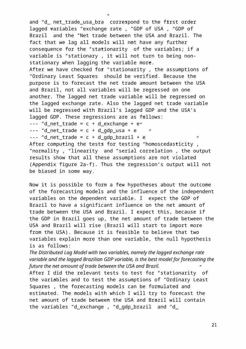
Figure 2f. Left the test for Heteroskedasticity and right the test for Linearity between the variablesd_net_trade and d_gdp_brazil.

Figure 3a-e, 4a-e:

Figure 3a. Correlogram of the errors of the AR Model Figure 4a. The Least Squares estimation of the

Coefficients of the AR Model.

21

Figure 3b. The test for serial correlation Figure 4b. The Least Squares estimation of theof the DL1 Model. Coefficients of the DL1 Model.

Figure 3c. The test for serial correlation Figure 4c. The Least Squares estimation of theof the DL2 Model with the Brazilian GDP as an extra Coefficients of the DL2 Model with the Brazilian GDP variable. as an extra variable.

Figure 3d. The test for serial correlation Figure 4d. The Least Squares estimation of theof the ARDL1 Model. Coefficients of the ARDL1 Model.

22

Figure 3e. The test for serial correlation Figure 4e. The Least Squares estimation of theof the ARDL2 Model with the Brazilian GDP as an Coefficients of the ARDL2 Model with the Brazilianextra variable. GDP variable as an extra variable.

23