Do Today’s Trades Affect Tomorrow’s IPO Allocations?

M. Nimalendran, Jay R. Ritter and Donghang Zhang∗

February 3, 2006

JLE classification: G24 Keywords: IPOs, brokerage commissions

∗ Nimalendran is from the Department of Finance, University of Florida, Gainesville, FL 32611-7168, Ritter is

from the University of Florida, and Zhang is from the Moore School of Business, University of South Carolina,

Columbia, SC 29208. Nimalendran can be reached at (352) 392-9526 or nimal@cba.ufl.edu. Ritter can be

reached at (352) 846-2837 or jay.ritter@cba.ufl.edu. Zhang can be reached at (803) 777-0242 or

zhang@moore.sc.edu. Zhang acknowledges financial support from the University of South Carolina Research

and Productive Scholarship Fund. We thank Shingo Goto, Kathleen Hanley, Paul Irvine, Mark Kamstra, Greg

Niehaus, Eric Powers, Sergey Tsyplakov, Kent Womack (the 2005 AFA discussant), an anonymous referee, and

seminar participants at the University of South Carolina and York University (Canada) for comments.

Do Today’s Trades Affect Tomorrow’s IPO Allocations?

Abstract

Underwriters using bookbuilding have discretionary power for allocating shares of initial public offerings (IPOs). Commissions paid to underwriters by investors are one of the determinants of IPO allocations. We test the hypothesis that investors trade liquid stocks in order to affect their IPO allocations. Consistent with this hypothesis, we find that money left on the table by IPOs affects the trading volume of the 50 most liquid stocks close to the offer date. For an IPO that leaves $1 billion on the table, in the six days ending on the day that trading commences there is abnormal volume in the 50 most liquid stocks of 2.7 to 4.1%, although only during the internet bubble period is this statistically significant.

1

Do Today’s Trades Affect Tomorrow’s IPO Allocations?

1. Introduction

Underwriters have discretion in allocating shares of initial public offerings (IPOs)

when bookbuilding is used. There are three main theories describing the allocation of shares

by investment bankers: 1) the academic view, 2) the pitchbook view, and 3) the profit-sharing

view. The academic view, exposited by Benveniste and Spindt (1989), argues that IPO

allocations are the solution to a mechanism design problem in which regular (i.e., institutional)

investors must be given inducements to honestly reveal their private information about the

valuation of a firm going public. The pitchbook view, exposited by investment bankers in

their presentations to prospective issuing firms, emphasizes that shares will be allocated to

buy-and-hold investors, as proxied by institutions that already are large holders of similar

firms. The profit-sharing view, exposited by Loughran and Ritter (2002, 2004) and Reuter

(2006), argues that hot IPOs are allocated to investors who direct commission business to the

investment banking firm in return. This paper tests an implication of the profit-sharing view

of IPO allocations.

From 1993 to 2001, the 3,499 firms going public left more than $93.5 billion on the

table, where the amount of money left on the table is defined as the number of shares offered

times the difference between the first-day closing price and the offer price. During 1999 and

2000, the internet bubble period, the 803 IPOs left a total of $63.5 billion on the table. During

this period, the average IPO had a first-day return of 65% and left $79 million on the table.

When such large wealth transfers are occurring, it is natural to assume that rent-seeking

activity will take place. When IPOs are routinely oversubscribed, and underwriters have

discretion in allocating shares, underwriters can boost their profits through a quid pro quo

arrangement by giving large allocations to investors who are willing to offer benefits to the

underwriter.

2

Consistent with the profit-sharing view, regulatory settlements indicate that investment

banks allocate IPOs partly on the basis of the trading commissions generated by institutional

investors.1 For example, the January 22, 2002 Securities and Exchange Commission (SEC)

settlement with Credit Suisse First Boston (CSFB) states that CSFB allocated hot IPOs to

some clients and in return received commissions of up to 65% of the clients’ profits within a

few days of the IPO.2 The clients kicked back part of their profits by paying unusually high

commissions on stock trading that in some cases had no other purpose than to generate

commissions. According to the Commission’s complaint, CSFB’s clients paid as high as $3.00

per share in commissions for block trades executed by CSFB brokers, although the usual

commission for institutional investors at the time was 6¢ per share (Goldstein, Irvine, Kandel,

and Wiener (2006)). CSFB paid a fine of $100 million and settled the case with the SEC

(without admitting or denying wrongdoing).

On January 9, 2003, the former Robertson Stephens securities unit of FleetBoston

Financial Corp. also settled similar accusations with the SEC and the National Association of

Securities Dealers (NASD) and paid a fine of $28 million. Beginning on November 17, 1997,

Robertson Stephens used an explicit formula to allocate IPO shares.3 “The Syndicate

Department generally allocated shares by using a formula that was weighted over the course

1 Although we focus on institutional trading, allocations of IPOs to individuals are also based partly on

commissions. For example, in September 2005, according to its website the policy of Charles Schwab, Inc. was

to restrict IPO allocations to clients who either i) had a $100,000 balance in their Schwab brokerage account(s),

or ii) had a $50,000 balance and had made at least 40 trades during the prior 12 months. 2 See SEC press release 2002-14 and the SEC complaint against CSFB for allegations on CSFB IPO allocations. In its January 22, 2002 news release (http://www.nasd.com), NASD Regulation, Inc. states that "CSFB's IPO

profit sharing practice was widespread, occurring between April 1999 and June 2000. The practice affected more

than 300 accounts serviced by the firm's Institutional Sales Trading Desk, its Private Client Services (PCS)

Group and its PCS Technology Group" and that "… during the last quarter of 1999, over 3,000 trades were done

at these excessive commission rates and hundreds of them were executed with a commission rate of $1 per share

or more." 3 See Michael Siconolfi and Anita Raghavan, “Robertson Stephens Tries to Stop ‘Spinning’ of Hot IPOs,” Wall

Street Journal November 18, 1997.

3

of 18 months in favor of those accounts that generated commissions closer in time to the IPO.

This formula was used to calculate a customer’s ‘Syndicate Rank’. …The Syndicate

Department also had discretion to allocate some IPO shares independent of the Syndicate

Rank on a case-by-case basis.”4

Robertson Stephens Inc. and CSFB are apparently not the only investment banks that

allocated IPOs on the basis of commission business. Reuter (2006) reports that for IPOs

underwritten by different investment banks from 1996 to 1999, a fund manager’s holding of

an IPO shortly after the offering is positively related to its commission payments to the lead

underwriter of the IPO.

Goldstein et al (2006) posit that "...commissions constitute a convenient way of

charging...for...timely access to information, priority handling of difficult trades and higher

allocations of IPO shares." SEC Commissioner Paul Atkins has publicly stated that it is

permissible for IPO allocations to be based on customer “relationships”.5 If the linkage

between allocations of underpriced IPOs and commission business is too direct, however, then

it is a violation of certain securities laws and regulations and self-regulatory organization rules

such as NASD Rule 2330. This rule prohibits an NASD member firm from sharing, directly

or indirectly, in the profits or losses in any account of a customer.

To date, the finance literature has not addressed the economic consequences of

allocating IPOs in return for commission business. To the degree that some of the money left

on the table flowed back to underwriters through either implicit or explicit profit-sharing

arrangements, this would suggest that the structure of the underwriting industry allowed i)

some underwriters to achieve total compensation that exceeded competitive levels, and/or ii)

issuers and their executives to receive additional benefits, such as optimistic analyst coverage

4 The quotation is from page 5 of the Acceptance, Waiver and Consent (AWC) No. CAF030001 submitted to the

NASD by Robertson Stephens. See press release 2003-3, the SEC complaint against Robertson Stephens, and the

AWC for details on the Robertson Stephens case. 5 As quoted in the Bloomberg News article of October 13, 2004 by Judy Mathewson, “U.S. SEC Proposes New

Initial Public Offering Rules.”

4

of their stock and favorable allocations of hot IPOs into personal brokerage accounts.

Although there is widespread agreement among practitioners that IPOs have been

allocated at least partly on the basis of commission business, it is unclear whether this was

based primarily on commissions paid over a long period of time or over a short period in

close proximity to specific IPOs.6 Furthermore, commission revenue is the product of shares

traded and the commission per share, and the impact of IPO-related trading on volume has not

been documented. Reuter (2006) finds that there is a positive relation between the

commissions paid to a given lead underwriter over a long period of time and the mutual

fund’s holdings of recent IPOs from that underwriter. Our paper examines the effect of money

left on the table by IPOs on the trading volume of the most liquid stocks in the days

surrounding the offer date. Thus, we are testing the joint hypothesis that i) money left on the

table in IPOs affects commission revenue, ii) some of the higher commission revenue occurs

through higher volume, and iii) there is a short-run effect on volume.

Bookbuilding, also known as a firm commitment contract, has been the dominant

method for selling IPOs in the U.S. for many years. All IPO allocation data are confidential in

the U.S., although there have been several academic studies utilizing such data (e.g.,

Aggarwal (2000), Boehmer, Boehmer, and Fishe (2005), and Hanley and Wilhelm (1995)).

The biggest obstacle for any research on this topic is the availability of detailed IPO allocation

and commission data.

In this study, we use an innovative empirical design to solve this data availability issue.

In the profit-sharing view of IPO allocations, an investor will receive a large allocation of a

hot IPO if it generates more commission revenue. To boost its commission ranking, an

investor may engage in stock churning, defined for the purposes of this paper as trading with

commission generation as the only intent. Other trading that an investor may engage in to

generate commissions is more subtle. For example, an investor could engage in portfolio

6 See, for example, Aaron Lucchetti, “SEC probes rates funds pay for commissions,” Wall Street Journal,

September 16, 1999, p. C1.

5

rebalancing and time the trading around IPO dates. An investor could also move routine

trading that is not time-sensitive to around IPO dates. For expositional convenience, we use

the term “IPO-related trading” for all trading with a whole or partial purpose of generating

commissions to affect IPO allocations.

If the purpose of IPO-related trading is to generate commissions that transfer profits

from IPO recipients back to the investment banking firm, there is an incentive to structure the

trades in a manner that minimizes the “leakage” to other market participants. Leakage can be

reduced by decreasing trading costs due to bid-ask spreads and price impact. A variety of

trading strategies could be employed to minimize this leakage. One mechanism would be to

simultaneously submit buy and sell orders for the identical block of stock with two different

securities firms. For almost all conceivable strategies, trading highly liquid stocks would be

preferred, in order to minimize bid-ask spreads and price impact costs, and to avoid the

attention that would come from trading a large block of a less liquid stock.

To capture IPO-related trading, we use the trading volume of the 50 most actively

traded stocks. We choose the top 50 stocks for each trading day based on the rank of a stock’s

average trading volume for the past 20 trading days, after excluding stocks with high

volatility or a price of below five dollars. For the 3,499 IPOs during our sample period from

1993 to 2001, we aggregate the money left on the table by IPOs by offer dates, and obtain a

time series of the daily amount of money left on the table. With controls for market

movements, a time trend, and calendar-related patterns in trading volume, we employ an

autoregressive model with four lags to study the relation between the daily trading volume of

the 50 most liquid stocks and the amount of money left on the table by IPOs. If short-run

commission generation is an important factor in IPO allocation, there should be a positive

relation between the amount of money left on the table and the trading volume of liquid

stocks around the IPO dates.

Because of changes in IPO practices, we partition our sample period into three

subperiods: the pre-internet bubble period (1993 – 1998), the internet bubble period (1999 –

6

2000), and the post-internet bubble period (2001). For all three subperiods, each $1 billion left

on the table during the six trading days beginning on day t generates abnormal volume in the

50 most liquid stocks of between 2.7% and 4.1% on day t.

The average amount of money left on the table during a six-day window for the three

subperiods is, respectively, $107 million, $756 million, and $72 million. Our point estimates

thus imply that IPO-related trading increased turnover in the 50 most actively traded stocks by

a statistically insignificant 0.4% during 1993-1998, a statistically significant 2.0% during

1999-2000, and a statistically insignificant 0.2% during 2001. Since the 50 most actively

traded stocks account for approximately 25% of aggregate market volume, if other stocks

were not affected by IPO-related trading, these numbers suggest that even during the bubble

years aggregate volume was boosted by only 0.5% by IPO-related trading. This suggests that

the effect on aggregate trading volume is economically insignificant in normal market

conditions, but had a statistically significant yet modest effect during the bubble years. This is

the central finding of our paper.

The commissions generated from the increase in the trading volume during the bubble

period are economically important. The extra trading volume of 2% per day for the liquid

stocks would result in an additional $656,000 per day in commissions if we assume an

average commission of 10¢ per share.7 This $656,000 per day in commissions, however,

represents only 0.52% of the $126 million per day left on the table during the bubble period, a

much lower payback ratio than the 30% or even 65% kickbacks revealed in the CSFB

regulatory case.

There are several reasons to believe that our estimate of the share of profits flowing

back to underwriters is biased downwards. Higher commissions can be generated by either

trading more shares or through higher commissions per trade. We only capture commissions

7 The average commission rate of 10¢ is based on a weighted average of 6¢ per share paid by mutual funds and 50¢ or more paid on some trades by hedge funds. Mutual funds received a much larger proportion of IPO

allocations than hedge funds did during our sample period.

7

generated by higher trading volume. In order to generate commissions at a given underwriter,

investors may simply direct trading to this underwriter rather than to another entity (such as

an electronic communication network (ECN) or crossing network), with no incremental

trading occurring. Investors may also trade less liquid stocks, but submit buy and sell orders

simultaneously with different brokers to mitigate the market impact. Most importantly, we

only measure the short-run trading volume that is induced by rent-seeking investors in pursuit

of IPO allocations.

Our findings complement those of Reuter (2006). Our empirical evidence suggests

that there is not only a relation between long-term commission business and IPO allocations

(Reuter’s finding), but also a short-run relation during the bubble period between the

aggregate amount of money left on the table and aggregate trading volume.

2. Data, the metric for IPO-related trading, and summary statistics

2.1. Data

We use the Securities Data Company’s (SDC) new issues database to identify IPOs

from 1993 to 2001. All unit offerings, American Depository Receipts (ADRs), Real Estate

Investment Trusts (REITs), and closed-end funds are excluded. We also exclude banks and

savings and loans (SIC 6020 – 6120 and 6712) and all IPOs with an offer price of less than $5.

We also exclude all IPOs that are not included in the Center for Research in Security Prices

(CRSP) database.8

The transaction data used to calculate trading volume for all stocks come from the

TAQ database. For each stock, transactions that were executed after the market close and/or

8 We use the CRSP database to check the IPO offer date and first-day closing price. The IPO offer dates reported

in the SDC database are often one day earlier than the actual first trading date (the pricing date usually is the day

before the actual trading date but after the market close). We use the date when the IPO first appears in the

CRSP database as the offer date when there is only a one-day difference between the SDC database and the

CRSP database. When the difference is more than one day apart, the New York Stock Exchange’s Trade and

Quote (TAQ) database and Yahoo! are used to verify the dates.

8

on regional exchanges are excluded because the liquidity conditions are usually worse in

aftermarket trading and/or on regional exchanges.

2.2. The metric for capturing IPO-related trading

We use the trading volume of the top 50 liquid stocks to capture IPO-related trading.

This metric is constructed as follows. First, for each trading day, we rank all stocks based on

the average of the past twenty trading days’ intra-day quote-to-quote return standard deviation.

Second, we exclude stocks with a price below $5 or with a volatility rank higher than 2,500,

where the stock with the lowest volatility has a rank of one. These screens eliminate roughly

two-thirds of CRSP-listed stocks on any given day. Stocks with a low price or high volatility

are unlikely to be good candidates for IPO-related trading because of their high risk and limits

on commissions per share paid on low priced stocks. Third, we calculate the share volume for

each remaining stock, during which transactions that were executed after the market close or

on regional exchanges are excluded. For stocks listed on NASDAQ, we divide the volume by

two to reflect the different conventions of reporting volume on NASDAQ versus the

American and New York Stock Exchanges. We then calculate the mean and standard deviation

of the daily volume for the past twenty trading days for each stock.

For any trading day, if the difference between a stock’s current trading volume and the

past twenty day’s average is more than four times greater than its past twenty-day standard

deviation of volume, the stock is excluded. This excludes about 3% of the sample. The reason

for doing so is because IPO-related trading is unlikely to increase a liquid stock’s daily

volume by this magnitude. Some non-IPO related reasons, such as stock splits or significant

news, may cause such dramatic increases in daily trading volumes. To minimize the noise in

our metric, we exclude those stocks for those specific days.

Finally, for each trading day (day t), all remaining stocks are ranked based on the past

twenty-day’s average daily volume. The 50 stocks with the highest volume are identified. We

use past volumes, instead of current volumes, to rank stocks to avoid any potential look-ahead

bias. The total trading volume of these 50 ranked stocks, denoted as TVOL50, is then used as

9

the metric to capture IPO-related trading on day t.

Although IPO-related trading is more likely to be associated with large liquid stocks,

our choice of the top 50 stocks is somewhat arbitrary. It is plausible that stocks ranked among

the top 200 or 500 could also be good candidates, especially when fund managers merely try

to time trading motivated by portfolio rebalancing to around IPO dates. Each top stock ranked

by trading volume would capture the IPO-related trading with a positive probability. But it is

plausible that the higher the rank, the higher the probability. Meanwhile, stock trading

volumes are very volatile, and the daily volume of any given stock has a lot of noise. So, if we

view the IPO-related trading as a signal we want to capture, we need to include a certain

number of stocks in our measure in order to increase the signal-to-noise ratio. The addition of

each stock along the rank of trading volume would potentially capture more of the

IPO-related trading, but at a decreasing rate. There are no clear rules that allow us to

determine the maximum signal-to-noise ratio. We use TVOL50 to try to achieve the

close-to-optimum signal-to-noise ratio.9

2.3. Summary statistics

We partition our sample period into three subperiods: the pre-internet bubble period

(1993 – 1998), the internet bubble period (1999 – 2000) and the post-internet bubble period

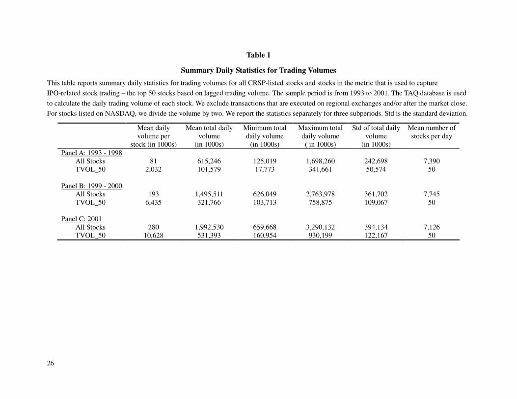
(2001). We report the summary statistics of daily trading volumes of all stocks and the 50

most liquid stocks in Table 1. For the three subperiods, the number of stocks traded per day

does not change much – 7,390 stocks for the pre-internet bubble period, 7,745 stocks for the

internet bubble period and 7,126 stocks for the post-internet bubble period. However, trading

volume has increased dramatically, partly due to stock splits and partly due to higher turnover.

For example, the mean daily total trading volumes of all stocks for the three subperiods are,

respectively, 615, 1,496, and 1,993 million shares (after dividing NASDAQ volume by two).

For the top 50 stocks (TVOL50), the mean daily total trading volumes are 102, 322, and 531

9 To make sure better metrics are not excluded, we also repeated our analysis using the top 30 stocks, or ranking

stocks based on both volume and the bid-ask spread. The results (not reported) are similar but slightly weaker.

10

million shares, respectively. The standard deviation of total daily trading volume has also

increased over time, although by a lower percentage than the mean has increased. Note that

the top 50 stocks are selected based on the past twenty day’s trading volume, and they do not

necessarily capture the most heavily traded 50 stocks of the current day.

The summary statistics for IPOs are reported in Table 2. We have 3,499 IPOs in the

nine-year sample period, of which 2,620 went public during the pre-internet bubble period,

803 went public during the internet bubble period, and only 76 went public during 2001. The

summary statistics for the whole sample and for the different subperiods that are reported in

Panel A of Table 2 are consistent with what has been reported in the literature. We also report

the daily summary statistics of our IPO sample in Panel B of Table 2. Except for the

post-internet bubble period, there are on average more than 1.5 IPOs per day, and there are

IPOs on more than half of the trading days. There is extreme variation in IPO activity from

day to day. For example, during the internet bubble period, the standard deviation of the

amount of money left on the table is $285 million per day, while the mean is only $126

million per day. Note that all of the money left on the table figures exclude the effect of

overallotment options, and the number of shares offered is measured as the domestic tranche

only. Thus, our estimates of the money left on the table are conservative.

Another noticeable feature about IPOs is the day of the week pattern, as shown in

Figure 1. The lead underwriter and the issuing firm usually finalize the offer price and allocate

shares to investors the day before trading starts. To avoid weekend uncertainties, IPOs rarely

start to trade on Mondays. For the other four weekdays, slightly more firms start trading on

Thursday and Friday. The first-day returns also demonstrate a day of the week pattern, with

mean first-day returns rising from Tuesday through Friday.10

10 The first-day returns on Mondays are dominated by a few outliers because of the small number of IPOs that

went public on Monday. The lower first-day returns on Tuesdays and Wednesdays relative to Fridays are

probably due to a tendency to delay deals on which there is buyer resistance from the latter part of the previous

week until Tuesday or Wednesday of the following week.

11

3. The effect of money left on the table on trading volume

3.1. The model

The summary statistics in Table 1 indicate that stock-trading volume is very volatile,

and the metric that we use to capture IPO-related trading is fairly noisy. During the internet

bubble period, for example, the coefficient of variation (standard deviation divided by the

mean) of total daily trading volume for the Top 50 stocks is 34 percent. Therefore, it is

important to control for the impact on trading volume of factors that are unrelated to IPO

activity. The literature on trading volume has focused on the contemporaneous relations

between volume and price movements (see e.g. Karpoff (1987), Campbell, Grossman, and

Wang (1992), He and Wang (1995), Andersen (1996), and Llorente, Michaely, Saar, and Wang

(2002)). To control for the time trend in volume, we use IndexDate _ as an explanatory

variable in our regressions, where IndexDate _ is the sequential number of each trading day

( t for day t ) divided by 2268, the total number of trading days in our sample period. (For

the rest of this paper, the value of a variable is measured on day t unless stated otherwise.)

The time series of trading volumes used in this paper is a stationary process after de-trending,

which is consistent with the literature (e.g., Andersen (1996) and Llorente et al (2002)).

The time series of TVOL50 also demonstrates a correlation with general market

conditions in addition to the time trend. We use the nominal level of the S&P 500 index to

control for this relation. The literature and the analysis of our data also suggest that trading

volumes demonstrate calendar-related patterns. IPO activity, as indicated in Figure 1, also

shows day of the week patterns. We use four weekday dummies (Tuesday through Friday) and

eleven month dummies (January through November) as controls for calendar-related patterns.

The volume literature suggests a strong relation between trading volume and price

volatility (Jones, Kaul, and Lipson (1994)). IPOs on the first day also have asymmetric betas

in up and down markets (Chan and Lakonishok (1992)). We use the S&P 500 index return and

12

its absolute value, mR and mR , to control for market-wide price movements. In sum, we

use the following autoregressive model:

εγ

δββ

ληηα

++

++++

+++=

��

�

=−

=

=

Money

VolumeRRMonthm

WeekdayPSIndexDateVolume

iiimm

iii

iii

*

****

*500&*_*

4

121

11

1

4

121

(1)

In the model, the dependent variable, Volume , is the natural log of TVOL50 for day t

multiplied by 100. This enables us to interpret any change of Volume in percentage terms.

Four lagged variables of Volume are used to remove the autoregressive part of the TVOL50

metric.11 The variable Money , measured in hundreds of millions of year 2000 dollars (year

2001 is unadjusted), is used to capture the money left on the table by IPOs in a window

around day t . We employ two different measures for the amount of money left on the table.

We first use the daily amount of money left on the table by IPOs for the day before the current

day ( 1−Money ), the current day ( 0Money ), and the next nine days ( 1+Money through

9+Money ). The second measure we use is the aggregate amount of money left on the table for

various window lengths around day t . If our hypothesis is correct, we would expect that the

coefficients on Money are positive.

The important goal for the use of daily money left on the table variables is to gauge

the timing of the impact of IPO activity on volume. We include one lagged money left on the

table variable for the daily IPO activity measure. Regulatory investigations of CSFB indicate

that commission payments from hedge funds peaked within a narrow window relative to when

some hot IPOs started trading, reflecting explicit profit-sharing agreements.12 We include the

11 This is the same approach that Naranjo and Nimalendran (2000) use to measure the unexpected trading

volume in the U.S. Dollar – German Deutsche Mark foreign exchange market. 12 Page 8 of the NASD Regulation, Inc. Letter of Acceptance, Waiver, and Consent No. CAF020001 with CSFB

states “Payment of inflated commissions ostensibly for brokerage services … involved at least 300 Customer

13

money left on the table on day 1t − to test whether it was a common practice for there to be

ex post profit-sharing after the IPO. The use of money on the table on day 1t + to day 9+t

is based on the assumption that institutional investors are able to forecast which IPOs will be

hot deals several days in advance, and that IPO allocations are affected by commissions

generated in the days immediately prior to the IPO. The “partial adjustment” literature as well

as discussions with industry participants suggests that this is a reasonable assumption.13

3.2. Regression results and analysis

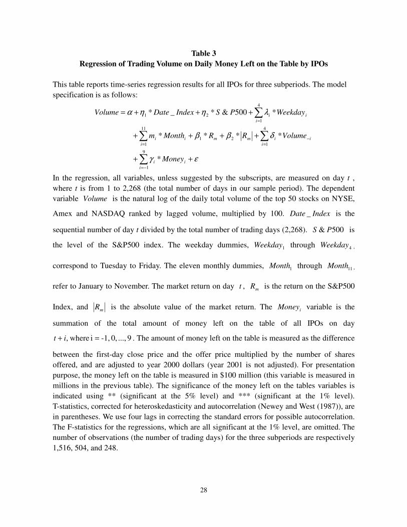
We estimate the regression model specified in equation (1) for the three subperiods.

The regression results for the daily IPO activity measures are reported in Table 3. The

coefficients for the control variables are consistent with our expectations. The positive

coefficients for IndexDate _ during the pre- and internet bubble periods capture the increase

in trading volume over time. 500& PS also explains part of the variation in trading volume

over time. The time variation in volume in 2001 is captured by IndexDate _ , 500& PS and

the eleven month dummies. Volume also increases when the market is volatile, and this is

captured by the significant coefficient for mR in all three subperiods. For example, the

coefficients on mR and mR for the pre-internet bubble period imply that a 1% daily

market return is associated with a 7.9% increase in volume relative to volume in a flat market.

The coefficient on mR is negative during the pre- and internet bubble periods, reflecting the

Accounts. During the last quarter of 1999, over 3000 trades were done at these excessive commission rates and

hundreds of trades were effected with a commission rate of $1.00 per share or more. …Over 90% of the

excessive commission transactions executed on the day of, the day before, or the day after a CSFB managed IPO,

were done by accounts that were allocated shares by CSFB in that hot IPO.” 13 In unreported results, we have analyzed the ability of forecasts of first-day returns made in an industry

newsletter (The IPO Reporter) to predict realized first-day returns on IPOs from 1998-2000. Each week, this

newsletter assigned an “opening consensus premium” on a scale of ¼ to 5+ for most IPOs during the following

two-to-three weeks. Almost all IPOs with first-day returns of 100% or more were given 5 or 5+ ratings several

weeks in advance of the offer date (frequently prior to the start of the road show).

14

asymmetric relation between volume and price movements in up and down markets. The first

two lags of the volume variable account for the autocorrelation in trading volume, consistent

with our expectations.

The money left on the table on the day before the current day (day 1t − ) has no

significant impact on the current day volume (day t volume) for all three subperiods. This

result indicates that explicit profit-sharing arrangements with ex post settling up allegedly

used by some members of the CSFB sales force were not a widespread practice. The money

left on the table variables for the rest of the ten days from t to 9+t display significantly

positive coefficients for some days during the pre- and the internet bubble periods. For the

pre-internet bubble period, only the coefficient for 2+Money is significant. For the internet

bubble period, the coefficients for 0Money , 1+Money and 5+Money are statistically

significant at the 1% or 5% levels. For no subperiods are any of the 6+Money to 9+Money

coefficients significantly different from zero. This suggests that money left on the table is

associated with higher abnormal trading volume during a six-day period prior to the IPO offer

date. This is consistent with the profit-sharing hypothesis. However, we find little support for

the profit-sharing hypothesis for the post-internet bubble period – none of the coefficients

during this period are significant. It should be noted that the regulatory scrutiny of IPO

allocation practices was first publicized in December 2000, so it is indeed possible that a

structural shift occurred. The coefficients for the money left on the table variables during the

internet bubble period suggest that IPOs affect the trading volume on and before the offer

dates, but that there is no evidence of ex post setting up.

Rather than focusing on each day separately, in Table 4 we aggregate the money left

on the table by IPOs for a rolling window of three different lengths: [ ]2, +tt , [ ]5, +tt and

[ ]9, +tt . We re-estimate the equation (1) regression model by replacing the daily money

variables with the aggregated variable. The coefficients for the control variables in Table 4 are

15

similar to those in Table 3, and are not reported. The coefficients for the aggregated money

left on the table variables with different aggregation windows are positive for all three

subperiods. They are only statistically significant for the internet bubble period, however. For

this subperiod, all three aggregated variables are significant at the 1% level. It should be noted

that the point estimates are similar for all three subperiods in Table 4, but the standard errors

are smaller in the internet bubble period because there is much more variation in the

explanatory variable as shown in Panel B of Table 2, allowing more precise parameter

estimates.

Besides statistical significance, the coefficients for the money left on the table

variables also suggest that IPO-related trading captured by liquid stocks is economically

important during the internet bubble period. To assess the economic importance, we assume

that new issues appear with an equal frequency and all days are average days and we use a

six-day aggregation window. Based on the numbers reported in Table 2, we would have $126

million (the mean daily amount of money left on the table) ∗ 6 (the number of days in the

window period) = $756 million left on the table for an arbitrarily chosen six-day window

during the internet bubble period. This indicates that IPO-related trading could cause a 0.27 ∗

756 / 100 = 2.04 percent increase in the trading volume on day t, where we divide by 100

because in the regressions the money left on the table is measured in $100 millions.

For the other two subperiods, our Table 4 point estimates imply that money left on the

table by IPOs during a six-day window increased turnover in the 50 most actively traded

stocks by a statistically insignificant 0.4% (mean daily money left on the table from Table 2 of

$18 million/100 * 6 days * 0.41) during 1993-1998 and 0.2% ($12 million per day /100 * 6

days * 0.29) during 2001.

On an average trading day during 1999-2000, the 2.04 percent increase in volume

attributable to rent-seeking activity would translate into 6.56 million shares and $656,000

additional commissions if the average per share commission is 10¢. For the three-day and the

ten-day windows, the incremental trading commissions on a 10¢ per share basis would be

16

$499,000 and $566,000, respectively. This is consistent with the regression results with daily

money left on the table variables. The ten-day window of [ ]9, +tt includes days beyond day

5+t for which money left on the table in the future does not have much impact on the

current day trading. This suggests that investors try to act during the week (five trading days)

in anticipation of a hot IPO, and that the six-day window better captures the impact of the

money left on the table on current day trading volume.

The above estimates are conservative. Our metric does not capture all IPO-related

trading, and the aggregated amount of money left on the table during a six-day window

affects not only the current day trading volume, but also the volume over a longer time period

when rent-seeking behavior is present (Reuter (2006)). But we believe that this is sufficient to

show that these numbers are economically not trivial. The regulatory settlements and

discussions with practitioners suggest that only hedge funds, which were allocated

approximately 7% of the shares in several of the IPOs featured in regulatory settlements,

regularly paid high per share commissions with explicit profit-sharing arrangements. Mutual

funds, which are regulated, are not alleged to have paid extremely high per share

commissions.

Our estimate that IPO-related rent-seeking activity during 1999-2000 led to a 2.04%

increase in the trading volume of the most liquid stocks is lower than the 10% increase in

aggregate trading volume that Ritter and Welch (2002) conjecture. This is partly due to the

fact that we purposely stay conservative in our above calculations, and we only measure

trading over a short period around the IPO. However, Ritter and Welch may overestimate the

effect of rent-seeking behavior on aggregate trading volume to the degree that trades that

would have occurred anyway are merely redirected to integrated securities firms that have hot

IPOs to allocate rather than to ECNs or other venues where there are no IPOs to hand out.

Furthermore, to the degree that profit sharing was implemented via higher commissions per

share rather than via extra trading, there would be a smaller effect on volume.

17

For the internet bubble period, the 2.04% increase in trading volume per day implies

only a 0.52% payback of the $126 million per day of money left on the table if we assume an

average commission of 10¢ per share. This estimate is far lower than the 30% or even 65%

payback ratios alleged in the CSFB regulatory settlement. Knowledgeable practitioners have

supplied to us “guesstimates” of the payback rate during the internet bubble ranging from a

low of 5% to a high of 30%. Our lower payback rate estimate is partly due to the fact that our

estimate is biased downwards. Specifically, wash sales and excessive trading of less liquid

stocks are not included, and we are only estimating the short-run relation. Our finding

suggests that most of the paybacks occurred over a longer time period. In other words,

commissions during the past year, instead of just this week’s commissions, affect next week’s

IPO allocations.

4. Are the results for the internet bubble period driven by changes in market

conditions?

Our regression results show that each $1 billion left on the table results in 2.7 to 4.1%

higher trading volume of the top 50 liquid stocks. However, one could argue that other factors

may be the driving force behind the coefficients on the money variables in equation (1). One

alternative hypothesis is that the information environment for the market varies over time.

When the overall dispersion of private information (disagreement among investors) is high,

trading will be more active. Meanwhile, the increased heterogeneity of opinions would also

induce higher IPO underpricing. This would induce a positive coefficient for the money

variable. Alternatively, investment banks and the issuing companies might prefer to time the

offering to coincide with a period when trading is active. This would also induce a positive

coefficient for the money variable in a regression setup such as that in equation (1).14

Both alternative hypotheses suggest that we could have an omitted variable problem.

14 We thank the anonymous referee and Kent Womack for suggesting these alternative hypotheses to us.

18

That is, besides the lagged volumes on the right hand side of the regressions, other market

condition variables could be correlated with the money variable, and omitting them could

cause the estimate of the money variable coefficient to be biased. To address these concerns,

in this section we perform two further tests: we re-estimate equation (1) with controls for

changes in the information environment and with controls for market timing.

4.1. Regression Results with Controls for Changes in the Information Environment

We use two measures to control for changes in the information environment. The first

measure we use is the logarithm of the daily return volatility for the past five days (day t-5 to

day t-1) of the top 50 liquid stocks, denoted as STDLN _ . Higher information asymmetry and

more active trading of the top 50 liquid stocks would be associated with higher volatility, so

we expect a positive coefficient for STDLN _ .

We use the estimator proposed by Parkinson (1980) to calculate the daily return

variance. This measure is constructed as follows. We first calculate the daily return variance

for each of the top 50 liquid stocks for the past five days using the daily high and low prices.

25

1

ln5361.0

_ �= −

−���

����

�=

iL

it

Hit

j PP

VARParkinson (2)

In equation (2), jVARParkinson _ is the variance of stock j measured over the past five days

(day t-5 to day t-1). HitP − and L

itP − are the intraday high and low prices of day it −

( 5,...,2,1=i ) for stock j. The advantage of the Parkinson extreme value method of calculating

stock variances is that it requires 80% less data compared to the traditional measures that use

the daily closing prices to achieve the same efficiency in the variance estimation. Using the

estimates for the individual stocks we calculate the equally weighted average of the daily

return variance for the top 50 stocks. Finally, we take the natural logarithm of the square root

of the average daily return variance. That is, on any given day t, STDLN _ is calculated as

follows:

19

��

���

= �

=

50

1

_501

ln_j

jVARParkinsonSTDLN (3)

The mean (standard deviation) for STDLN _ is -3.78 (0.23) for 1993-1998, -3.37 (0.24) for

1999-2000 and -3.18 (0.23) for 2001, respectively. Note that these statistics are expressed in

natural logarithms, and the average volatility (daily return standard deviation) for the three

subperiods is 2.28%, 3.44% and 4.16%, respectively.

The second measure, PESPRD , is the average percentage effective spread of the top

50 liquid stocks for the past five days. Higher information asymmetry would result in greater

bid-ask spreads for the top 50 liquid stocks. So we expect that PESPRD will capture the

time variation in the information environment.

The percentage effective bid-ask spread is estimated using the TAQ database. To

obtain the percentage effective spread, we first match each transaction with the latest quote

that is at least five seconds prior to the trade. The dollar effective spread is defined as the

absolute difference between the transaction price and the mid-point of the quote multiplied by

two. The percentage effective spread is the dollar effective spread scaled by the average of the

bid and ask quotes, expressed in percentages. We first calculate the daily average percentage

effective spread for each stock, and then calculate the average for the past five days. We

finally take the average of the percentage effective spread of the top 50 stocks for the past five

days to obtain PESPRD . For exposition purposes, we multiply PESPRD by 100 in the

regressions so that it is expressed in basis points.

The mean (standard deviation) for PESPRD (in basis points) is 15.34 (4.27) for

1993-1998, 8.60 (1.07) for 1999-2000 and 7.04 (2.16) for 2001, respectively. The decrease in

the mean value of the bid-ask spread from 1993-1998 to 1999-2000 is consistent with less

adverse selection due to a lower proportion of trading by informed investors, possibly due to

more churning. Since we expect less IPO-related churning in 2001, however, the continued

decrease in the mean value of the bid-ask spread cannot be plausibly explained by this. In

20

addition, the huge drop in the percentage bid-ask spread (by more than 50% from the first to

the last subperiod) is too large to be explained by merely an increase in IPO-related churning.

The regression model including the market condition variable(s) is as follows:

εθγ

δββ

ληηα

+++

++++

+++=

��

�

=−

=

=

tEnvironmenInfoMoneyAggregate

VolumeRRMonthm

WeekdayPSIndexDateVolume

iiimm

iii

iii

_*]5,0[_*

****

*500&*_*

4

121

11

1

4

121

(4)

We use the logged volatility and the percentage effective spread both separately and jointly to

replace the variable Info_Environment. The regression results are reported in Table 5. We only

report the results using the money left on the table over the six-day aggregation window. All

the control variables have similar coefficients to those reported in Table 3, and are not

reported. The coefficient on the logged volatility is always positive when used alone, and is

statistically significant for the pre- and post-internet bubble periods. The coefficient on the

percentage effective spread is positive when used alone, and is marginally significant during

the internet bubble period.

The Table 5 results suggest that, even though we control for contemporaneous market

returns, the information environment still has an impact on the current day’s trading volume.

For example, if the daily return volatility of the top 50 stocks is increased from 3.44% to

4.44% (approximately one standard deviation), this 1% increase from the mean, when used

alone to control for the changes in market conditions, would cause a statistically insignificant

0.92% increase in the current day’s trading volume during the internet bubble period.15 If the

percentage effective spread is used alone, an increase of 1 basis point (one standard deviation)

in the past five day’s average percentage effective spread would cause a marginally significant

15 0.92=3.59×ln(4.44/3.44), where 3.59 is the regression coefficient in the middle panel of Table 5. When

STDLN _ is included, the coefficient on || mR , which helps to capture the impact of the market-wide

volatility, is slightly reduced but remains significant at the 1% level.

21

1.19% increase in the current day’s trading volume. For all model specifications and all

subperiods, however, the coefficients for the money variable remain qualitatively unchanged

compared to those in Table 4. Furthermore, our results for the money left on the table

coefficients are robust to using three- or ten-day windows. This suggests that the relation

identified in Table 4 between the money left on the table and the volume of the top 50 liquid

stocks is not driven by changes in the information environment.

4.2. Regression Results with Controls for Market Timing

To further disentangle the market timing hypothesis and the profit sharing hypothesis,

we add another variable, the number of IPOs, in the regression model reported in Table 6:

εθγ

δββ

ληηα

+++

++++

+++=

��

�

=−

=

=

IPOsNumberMoneyAggregate

VolumeRRMonthm

WeekdayPSIndexDateVolume

iiimm

iii

iii

_*]5,0[_*

****

*500&*_*

4

121

11

1

4

121

(5)

The new variable, IPOsNumber _ , is the number of IPOs in our sample on day t . If the

relation between the volume of the top 50 liquid stocks and IPO activity is mainly driven by

investment banks’ market timing abilities, the number of IPOs would better capture this

relation than the money left on the table, which is jointly determined by the number of IPOs,

the size of the offerings and the underpricing. In other words, if the relation between volume

and IPO activity is driven by market timing rather than profit sharing, we would expect that

the coefficient on the money left on the table would be dramatically reduced.

We report the regression results in Table 6, where, as in Tables 4 and 5, we do not

report the coefficients on the control variables in the interest of brevity. For all three

subperiods, both the money left on the table and the number of IPOs are positively related to

the volume of the top 50 liquid stocks. The coefficients on the number of IPOs and the money

left on the table are only significant, at the 5% level and the 1% level, respectively, during the

internet bubble period. Most importantly, the inclusion of this additional variable has only a

22

modest effect on the coefficient of the money left on the table variable during 1999-2000,

reducing it from the 0.27 (t=3.99) that we report in Tables 4 and 5 to 0.21 (t=3.34) in Table 6.

This suggests that the profit sharing we observe during the internet bubble period is not

entirely driven by market timing.

The number of IPOs, however, is economically just as important as the money left on

the table in explaining the volume of the 50 most liquid stocks. Since the coefficient on the

number of IPOs during the bubble period is 0.99, and there are 1.59 IPOs per day on average,

the difference in volume between an average day and a day with zero IPOs is 1.57%. This is

approximately the same effect as money left on the table: the coefficient of 0.21 implies that

there is a difference of 1.59% in volume between an average day (where the money left on the

table variable has a value of $756 million) and a day with zero money left on the table.

5. Conclusion

In recent years the vast majority of IPOs have been marketed using the bookbuilding

process. This process gives the lead underwriter considerable discretion in setting the offer

price and allocating shares of the issuing firm. Academic researchers have generally assumed

that the lead underwriter uses this allocation discretion in the best interest of the issuer to

mitigate information asymmetry. However, recent regulatory investigations, as well as

discussions with practitioners, indicate that allocations of underpriced shares are at least partly

based on commission business from investors.

Commission revenue equals the product of shares traded and the commission per share.

Commission revenue can be tabulated over short periods immediately surrounding IPOs

(high-frequency data) or over longer periods (low-frequency data). This paper examines

whether there is a high-frequency relation between the money left on the table by IPOs and

trading volume. IPO allocation data are confidential, and we use an indirect measure of

abnormal commission revenue – the abnormal trading volume of liquid stocks – to capture

IPO-related trading.

23

We find that $1 billion left on the table during the six trading days commencing with

day t (days t to t+5 ) generates abnormal volume in the 50 most liquid stocks of between

2.7% and 4.1% on day t, although only during the internet bubble period is this point estimate

reliably different from zero. This relation between the money left on the table and abnormal

trading volume on liquid stocks just prior to the offer date suggests that the gross spread is not

the only source of compensation for IPO underwriters.

Our point estimates imply that during 1999-2000 the trading volume of the 50 most

liquid stocks was 2.0% higher than it would have been if rent-seeking behavior was not

occurring. Since these stocks represented about 25% of aggregate trading volume, this would

suggest that aggregate volume was boosted by 0.5%, a much lower number than the 10%

increase that Ritter and Welch (2000) conjectured.

Our results are consistent with the profit sharing hypothesis that during the bubble

period, rent-seeking activity occurred whereby securities firms with hot IPOs to allocate

received commission revenue from investors in return for favorable IPO allocations. Our

finding of only modest effects on trading volume suggests that to the extent that significant

commissions flowed to the brokerage firms in return for favorable IPO allocations, the data

indicate that the main instrument was the commission per share rather than trading volume.

Furthermore, our finding that trading in the 50 most liquid stocks rises only modestly

immediately prior to money being left on the table suggests that the IPO allocations were

primarily determined by low-frequency commission business as suggested by Reuter (2006)

and/or explicit profit sharing arrangements using high commissions per share, rather than the

high-frequency trading volume relations that we investigate.

Other evidence corroborates this interpretation. Institutional trading volume did not

fall dramatically in the post-2000 years, even though less money has been left on the table by

IPOs. Furthermore, average institutional commissions per share have fallen from 5.9 cents per

share in 2000 to 4.7 cents per share in 2004, according to data from Greenwich Associates

reported in Goldstein et al (2006).

24

References

Aggarwal, Reena, 2000, Stabilization activities by underwriters after initial public offerings,

Journal of Finance 55, 1075-1103.

Andersen, Torben G.., 1996, Return volatility and trading volume: An information flow interpretation of stochastic volatility, Journal of Finance 51, 169-204.

Benveniste, Lawrence M., and Paul A. Spindt, 1989, How investment bankers determine the offer price and allocation of new issues, Journal of Financial Economics 24, 343-361.

Boehmer, Beatrice, Ekkehart Boehmer, and Raymond P. H. Fishe, 2005, Do institutions receive favorable allocations in IPOs with better long run returns? Journal of Financial and Quantitative Analysis, forthcoming.

Campbell, John Y., Sanford J. Grossman, and Jiang Wang, 1992, Trading volume and serial correlation in stock returns, Quarterly Journal of Economics 108, 905-939.

Chan, Louis, and Joseph Lakonishok, 1992, Robust measurement of beta risk, Journal of Financial and Quantitative Analysis 27, 265-282.

Chen, Hsuan-Chi, and Jay R. Ritter, 2000, The seven percent solution, Journal of Finance 55, 1105-1131.

Cliff, Michael, and David Denis, 2004, Do IPO firms purchase analyst coverage with underpricing? Journal of Finance 59, 2871-2901.

Goldstein, Michael, Paul Irvine, Eugene Kandel, and Zvi Wiener, 2006, Brokerage commissions and institutional trading patterns, Babson College working paper.

Hanley, Kathleen Weiss, and William J. Wilhelm, Jr., 1995, Evidence on the strategic allocation of initial public offerings, Journal of Financial Economics 37, 239-257.

He, Hua, and Jiang Wang, 1995, Differential information and dynamic behavior of stock trading volume, Review of Financial Studies 8, 919-972.

Jones, Charles M., Gautum Kaul, and Marc L. Lipson, 1994, Transactions, volume, and volatility, Review of Financial Studies 7, 631-651.

Karpoff, Jonathan M., 1987, The relation between price changes and trading volume: A survey, Journal of Financial and Quantitative Analysis 22, 109-126.

Llorente, Guillermo, Roni Michaely, Gideon Saar, and Jiang Wang, 2002, Dynamic volume-return relation of individual stocks, Review of Financial Studies 15, 1005-1047.

Loughran, Tim, and Jay R. Ritter, 2002, Why don’t issuers get upset about leaving money on the table in IPOs? Review of Financial Studies 15, 413-443.

25

Loughran, Tim, and Jay R. Ritter, 2004, Why has IPO underpricing changed over time? Financial Management 33 (3), 5-37.

Luccetti, Aaron, 1999, SEC probes rates funds pay for commissions, Wall Street Journal, September 16 issue, C1.

Mathewson, Judy, 2004, U.S. SEC proposes new initial public offering rules, Bloomberg News, October 13.

Naranjo, Andy, and M. Nimalendran, 2000, Government intervention and adverse selection costs in foreign exchange markets, Review of Financial Studies 13, 453-477.

Newey, Whitney K., and Kenneth D. West, 1987, A simple, positive semi-definite, heteroskedasticity and autocorrelation consistent covariance matrix, Econometrica 55, 703-708.

Parkinson, Michael, 1980, The extreme value method for estimating the variance of the rate of return, Journal of Business 53, 61-65.

Reuter, Jonathan, 2006, Are IPO allocation for sale? Evidence from the mutual fund industry, Journal of Finance, forthcoming.

Ritter, Jay R., and Ivo Welch, 2002, A review of IPO activity, pricing, and allocations, Journal of Finance 57, 1795-1828.

The IPO Reporter, 1998-2000, New York: Thomson Financial.

26

Table 1

Summary Daily Statistics for Trading Volumes This table reports summary daily statistics for trading volumes for all CRSP-listed stocks and stocks in the metric that is used to capture IPO-related stock trading – the top 50 stocks based on lagged trading volume. The sample period is from 1993 to 2001. The TAQ database is used to calculate the daily trading volume of each stock. We exclude transactions that are executed on regional exchanges and/or after the market close. For stocks listed on NASDAQ, we divide the volume by two. We report the statistics separately for three subperiods. Std is the standard deviation.

Mean daily volume per

stock (in 1000s)

Mean total daily volume

(in 1000s)

Minimum total daily volume

(in 1000s)

Maximum total daily volume ( in 1000s)

Std of total daily volume

(in 1000s)

Mean number of stocks per day

Panel A: 1993 - 1998 All Stocks 81 615,246 125,019 1,698,260 242,698 7,390 TVOL_50 2,032 101,579 17,773 341,661 50,574 50 Panel B: 1999 - 2000 All Stocks 193 1,495,511 626,049 2,763,978 361,702 7,745 TVOL_50 6,435 321,766 103,713 758,875 109,067 50 Panel C: 2001 All Stocks 280 1,992,530 659,668 3,290,132 394,134 7,126 TVOL_50 10,628 531,393 160,954 930,199 122,167 50

27

Table 2 Summary Statistics on IPOs

This table reports summary statistics for the IPO sample for the sample period from 1993 to 2001 and for three subperiods. Panel A of the table reports descriptive statistics of the IPO sample, and Panel B reports daily statistics. The first-day return is defined as the return from the offer price to the first-day close price. Money left on the table is defined as the difference between the offer price and the first-day close price multiplied by the number of shares offered (domestic tranche only), assuming no exercise of overallotment options. Both the proceeds and the money left on the table are adjusted using the CPI to year 2000 dollars (year 2001 is not adjusted). Positive IPOs refer to the IPOs that have positive first-day returns. In Panel B, all daily statistics are unconditional, except for the amount of money left on the table in the last row, which is conditioning on at least one IPO on that day.

Overall 93-98 99-00 2001

Panel A:

Number of IPOs 3,499 2,620 803 76

Mean number of shares offered (‘000) 5,282 3,869 7,981 25,459

Mean proceeds (million dollars) 99.18 71.73 155.80 446.92

Mean first-day return (%) 27.11 15.87 64.96 14.44

Mean money left on the table (million dollars)

26.73 10.33 79.04 39.04

Panel B:

Number of Trading Days 2,268 1,516 504 248

Number of Days with IPOs 1,288 953 278 57

Mean Number of IPOs per Day 1.54 1.73 1.59 0.31

Mean Number of Positive IPOs per Day 1.21 1.34 1.31 0.25

Mean Daily Money Left on the Table (million dollars)

41.23 17.86 125.93 11.97

Standard Deviation of Daily Money Left on the Table (million dollars)

146.95 43.20 284.86 51.49

Minimum Daily Money Left on the Table (million dollars)

-276.52 -7.67 -276.52 -36.11

Maximum Daily Money Left on the Table (million dollars)

2608.72 518.49 2608.72 616.31

Mean Daily Money Left on the Table Conditioning on at least 1 IPO (million dollars)

72.60 28.41 228.30 52.06

28

Table 3 Regression of Trading Volume on Daily Money Left on the Table by IPOs

This table reports time-series regression results for all IPOs for three subperiods. The model specification is as follows:

εγ

δββ

ληηα

++

++++

+++=

�

��

�

−=

=−

=

=

9

1

4

121

11

1

4

121

*

****

*500&*_*

iii

iiimm

iii

iii

Money

VolumeRRMonthm

WeekdayPSIndexDateVolume

In the regression, all variables, unless suggested by the subscripts, are measured on day t , where t is from 1 to 2,268 (the total number of days in our sample period). The dependent variable Volume is the natural log of the daily total volume of the top 50 stocks on NYSE,

Amex and NASDAQ ranked by lagged volume, multiplied by 100. IndexDate _ is the

sequential number of day t divided by the total number of trading days (2,268). 500& PS is

the level of the S&P500 index. The weekday dummies, 1Weekday through 4Weekday ,

correspond to Tuesday to Friday. The eleven monthly dummies, 1Month through 11Month ,

refer to January to November. The market return on day t , mR is the return on the S&P500

Index, and mR is the absolute value of the market return. The iMoney variable is the

summation of the total amount of money left on the table of all IPOs on day

9 ..., 0, -1,i where, =+ it . The amount of money left on the table is measured as the difference

between the first-day close price and the offer price multiplied by the number of shares offered, and are adjusted to year 2000 dollars (year 2001 is not adjusted). For presentation purpose, the money left on the table is measured in $100 million (this variable is measured in millions in the previous table). The significance of the money left on the tables variables is indicated using ** (significant at the 5% level) and *** (significant at the 1% level). T-statistics, corrected for heteroskedasticity and autocorrelation (Newey and West (1987)), are in parentheses. We use four lags in correcting the standard errors for possible autocorrelation. The F-statistics for the regressions, which are all significant at the 1% level, are omitted. The number of observations (the number of trading days) for the three subperiods are respectively 1,516, 504, and 248.

29

Variable 1993 – 1998 1999 - 2000 2001

791.78 976.34 1,789.51 Intercept (13.20) (7.99) (4.09) 55.20 311.33 -106.34 IndexDate _ (7.54) (7.68) (-0.32)

0.03 -0.06 -0.08 500& PS (5.41) (-2.70) (-1.76)

15.57 6.62 14.57 Tuesday (11.03) (2.86) (4.62)

17.38 8.00 17.91 Wednesday (12.18) (3.57) (5.01)

11.86 4.77 15.63 Thursday (8.22) (2.08) (6.12)

6.54 -2.16 7.16 Friday (3.44) (-0.70) (1.47)

12.57 18.85 6.11 January (4.18) (2.90) (0.20)

9.83 6.39 -0.11 February (3.31) (1.27) (-0.00)

9.06 11.46 0.76 March (3.14) (2.07) (0.03)

9.39 16.08 1.36 April (3.21) (2.66) (0.06)

5.14 1.65 -8.96 May (1.78) (0.28) (-0.45)

3.17 2.00 -11.47 June (1.13) (0.33) (-0.70)

5.02 0.75 -20.37 July (1.62) (0.12) (-1.65)

3.68 -3.51 -28.23 August (1.27) (-0.57) (-2.65)

5.79 0.89 -4.56 September (1.96) (0.16) (-0.48)

8.52 6.05 -8.94 October (2.84) (1.34) (-1.22)

3.59 1.38 -8.11 November (1.02) (0.27) (-1.16)

-0.78 -0.57 1.02 mR (-1.80) (-1.32) (1.68)

8.68 4.40 4.95 mR

(10.20) (6.03) (4.49)

30

Table 3 Continued: Variable 1993 – 1998 1999 - 2000 2001

0.41 0.34 0.34 1−Volume (10.87) (6.62) (5.06)

0.08 0.08 -0.10 2−Volume (2.96) (1.79) (-1.28)

0.03 0.01 -0.06 3−Volume (1.21) (0.22) (-0.74)

0.01 -0.02 0.02 4−Volume (0.59) (-0.53) (0.28)

-0.74 -0.12 1.88 1−Money (-0.76) (-0.57) (1.00)

0.02 0.70*** -1.12 0Money (0.02) (3.50) (-0.87)

-0.31 0.45*** 0.68 1+Money (-0.38) (2.98) (0.57)

2.30*** -0.04 -0.61 2+Money (2.79) (-0.24) (-0.33)

-0.22 0.29 0.56 3+Money (-0.28) (1.51) (0.41)

1.48 0.02 -1.88 4+Money (1.50) (0.10) (-1.41)

-0.87 0.41** -1.69 5+Money (-0.72) (2.27) (-0.85)

-0.11 -0.13 -0.62 6+Money (-0.14) (-0.68) (-0.55)

1.29 -0.02 -0.66 7+Money (1.27) (-0.13) (-0.52)

1.00 0.04 -0.80 8+Money (1.18) (0.23) (-0.61)

-1.51 -0.22 1.01 9+Money (-1.13) (-1.09) (0.64)

31

Table 4 Regression of Trading Volume on Aggregate Money Left on the Table by IPOs

This table reports time-series regression results for all IPOs for three subperiods. The model specification is as follows:

εγ

δββ

ληηα

++

++++

+++=

��

�

=−

=

=

],[_*

****

*500&*_*

4

121

11

1

4

121

jiMoneyAggregate

VolumeRRMonthm

WeekdayPSIndexDateVolume

iiimm

iii

iii

In the regression, the dependent variable, Volume , which is the natural log of the daily total volume of the top 50 stocks on NYSE, Amex and NASDAQ ranked by lagged volume, multiplied by 100, is the same as in Table 3. All the control variables are also the same as those in Table 3. For the measure of money left on the table, we use the aggregated amount of

money left on the table (measured in units of $100 million) from day it + to day jt + .

Three different aggregation windows around day t (i.e., 0=i ) are used.

]2,0[_ MoneyAggregate is the aggregate amount of money left on the table by IPOs over a

window of ]2,[ +tt , for example. The other two measured are similarly denoted. The

coefficients for all the control variables are similar to the ones reported in Table 3 and are omitted. The significance of the aggregate money left on the tables variables is indicated using *** (significant at the 1% level). T-statistics, corrected for heteroskedasticity and autocorrelation (Newey and West (1987)), are in parentheses. We use four lags in correcting the standard errors for possible autocorrelation. The F-statistics for the regressions, which are all significant at the 1% level, are omitted. The number of observations (the number of trading days) for the three subperiods are respectively 1,516, 504, and 248. Variable 1993 – 1998 1999 - 2000 2001

0.72 0.41*** 0.76 tMoneyAggregate ]2,0[_

(1.41) (3.64) (0.60)

0.41 0.27*** 0.29 tMoneyAggregate ]5,0[_

(1.32) (3.99) (0.30)

0.29 0.14*** 0.43 tMoneyAggregate ]9,0[_ (1.17) (3.25) (0.50)

32

Table 5 Regression of Trading Volume on Aggregate Money Left on the Table by IPOs with Controls

for Information Environment Change The model specification is as follows:

εθγ

δββ

ληηα

+++

++++

+++=

��

�

=−

=

=

tEnvironmenInfoMoneyAggregate

VolumeRRMonthm

WeekdayPSIndexDateVolume

iiimm

iii

iii

_*]5,0[_*

****

*500&*_*

4

121

11

1

4

121

The regression model is identical to that reported in Table 4, except that we add the variable(s)

tEnvironmenInfo _ as a control for the changes in the information environment. We use two

variables, the logarithm of the equally weighted daily return standard deviation ( STDLN _ ) of the

50 most liquid stocks for the past five days relative to day t ( t -5 to 1−t ) and the average percentage effective spread for the past five days ( PESPRD , expressed in basis points) for the 50 most liquid stocks. We follow Parkinson (1980) to estimate the return standard deviation. In the table below we report the coefficients for the aggregated money variables (measured in units of $100 million) and the market condition variables only. The coefficients for all of the other control variables are similar to those reported in Table 3. The significance of the variables is indicated using *** (significant at the 1% level), ** (significant at the 5% level), and * (significant at the 10% level). T-statistics, corrected for heteroskedasticity and autocorrelation (Newey and West (1987)), are in parentheses. Subperiod Variable No Control for

Info_Environment With

STDLN _ With

PESPRD With Both

0.41 0.44 0.39 0.44 tMoneyAggregate ]5,0[_ (1.32) (1.41) (1.26) (1.40)

9.71*** 12.30*** STDLN _ (3.25) (3.62)

0.07 -0.46

1993-1998

PESPRD (0.23) (-1.33)

0.27*** 0.28*** 0.30*** 0.30*** tMoneyAggregate ]5,0[_ (3.99) (4.24) (4.37) (4.38)

3.59 -0.51 STDLN _ (0.68) (-0.09)

1.19* 1.24*

1999-2000

PESPRD (1.74) (1.78)

0.29 0.26 0.29 0.24 tMoneyAggregate ]5,0[_ (0.30) (0.27) (0.30) (0.25)

19.86* 24.17** STDLN _ (1.88) (2.00)

0.04 -1.78

2001

PESPRD (0.02) (-0.93)

33

Table 6 Regression of Trading Volume on Aggregate Money Left on the Table by IPOs and Number of

IPOs The model specification is as follows:

εθγ

δββ

ληηα

+++

++++

+++=

��

�

=−

=

=

IPOsNumberMoneyAggregate

VolumeRRMonthm

WeekdayPSIndexDateVolume

iiimm

iii

iii

_*]5,0[_*

****

*500&*_*

4

121

11

1

4

121

Compared to the regression in Table 4, the additional variable IPOsNumber _ is the number of

IPOs on day t . In this table we report the coefficients for the aggregated money (measured in

units of $100 million) variables and the variable IPOsNumber _ . The coefficients for all of the

other control variables are not reported. The significance of the variables is indicated using *** (significant at the 1% level) and ** (significant at the 5% level). T-statistics, corrected for heteroskedasticity and autocorrelation (Newey and West (1987)), are in parentheses. Variable 1993-1998 1999-2000 2001

0.38 0.21*** 0.15 tMoneyAggregate ]5,0[_ (1.29) (3.34) (0.16)

0.07 0.99** 2.18 IPOsNumber _ (0.23) (2.39) (1.50)

34

Figure 1 Day of the Week Pattern of IPOs

This figure demonstrates the existence of a day of the week pattern in both the number of deals and the average first-day return for IPOs. We group IPOs by year. Figures 1.1 and 1.2 report the number of IPOs and the mean first-day return on different weekdays, respectively. For each year in each figure, one bar represents one weekday from Monday through Friday from left to right. Over the sample period, the mean first-day return and the number of IPOs on each weekday are as follows: 35.87% and 44 (Monday), 24.57% and 719 (Tuesday), 25.83% and 737 (Wednesday), 23.93% and 916 (Thursday), and 31.99% and 1,083 (Friday). Because of relatively few IPOs on Monday, the mean first-day return of Monday is sensitive to outliers (for example, there are only two IPOs on Monday for year 2000, and the average first-day return is 258%). For expositional purposes, the first-day return on Monday is set as zero in Figure 1.2.

Figure 1.1 Day of the Week Pattern for IPOsNumber of IPOs

0

50

100

150

200

250

1993 1994 1995 1996 1997 1998 1999 2000 2001

Figure 1.2 Day of the Week Pattern for IPOsMean First-Day Returns (%) (Return on Monday is set to zero)

0

10

20

30

40

50

60

70

80

1993 1994 1995 1996 1997 1998 1999 2000 2001