Distributed Algorithms 2020 - Jukka Suomela

DistributedAlgorithms 2020Juho Hirvonen and Jukka SuomelaAalto University, Finland

https://jukkasuomela.fi/da2020/

December 11, 2021


Contents

Foreword viii

About the Course . . . . . . . . . . . . . . . . . . . . . . . . viiiAcknowledgments . . . . . . . . . . . . . . . . . . . . . . . . ixWebsite . . . . . . . . . . . . . . . . . . . . . . . . . . . . . . ixLicense . . . . . . . . . . . . . . . . . . . . . . . . . . . . . . ix

Part I Informal Introduction

1 Warm-Up 2

1.1 Running Example: Coloring Paths . . . . . . . . . . . . 21.2 Challenges of Distributed Algorithm . . . . . . . . . . . 31.3 Coloring with Unique Identifiers . . . . . . . . . . . . . 41.4 Faster Coloring with Unique Identifiers . . . . . . . . . . 7

1.4.1 Algorithm Overview . . . . . . . . . . . . . . . . 81.4.2 Algorithm for One Step . . . . . . . . . . . . . . 81.4.3 An Example . . . . . . . . . . . . . . . . . . . . 91.4.4 Correctness . . . . . . . . . . . . . . . . . . . . 111.4.5 Iteration . . . . . . . . . . . . . . . . . . . . . . 11

1.5 Coloring with Randomized Algorithms . . . . . . . . . . 121.5.1 Algorithm . . . . . . . . . . . . . . . . . . . . . 121.5.2 Analysis . . . . . . . . . . . . . . . . . . . . . . 121.5.3 With High Probability . . . . . . . . . . . . . . . 13

1.6 Summary . . . . . . . . . . . . . . . . . . . . . . . . . 131.7 Quiz . . . . . . . . . . . . . . . . . . . . . . . . . . . . 141.8 Exercises . . . . . . . . . . . . . . . . . . . . . . . . . . 141.9 Bibliographic Notes . . . . . . . . . . . . . . . . . . . . 16

i

1.10 Appendix: Mathematical Preliminaries . . . . . . . . . . 161.10.1 Power Tower . . . . . . . . . . . . . . . . . . . . 161.10.2 Iterated Logarithm . . . . . . . . . . . . . . . . 17

Part II Graphs

2 Graph-Theoretic Foundations 19

2.1 Terminology . . . . . . . . . . . . . . . . . . . . . . . . 192.1.1 Adjacency . . . . . . . . . . . . . . . . . . . . . 192.1.2 Subgraphs . . . . . . . . . . . . . . . . . . . . . 202.1.3 Walks . . . . . . . . . . . . . . . . . . . . . . . 202.1.4 Connectivity and Distances . . . . . . . . . . . . 222.1.5 Isomorphism . . . . . . . . . . . . . . . . . . . . 24

2.2 Packing and Covering . . . . . . . . . . . . . . . . . . . 242.3 Labelings and Partitions . . . . . . . . . . . . . . . . . . 272.4 Factors and Factorizations . . . . . . . . . . . . . . . . . 292.5 Approximations . . . . . . . . . . . . . . . . . . . . . . 312.6 Directed Graphs and Orientations . . . . . . . . . . . . 312.7 Quiz . . . . . . . . . . . . . . . . . . . . . . . . . . . . 322.8 Exercises . . . . . . . . . . . . . . . . . . . . . . . . . . 332.9 Bibliographic Notes . . . . . . . . . . . . . . . . . . . . 35

Part III Models of Computing

3 PN Model: Port Numbering 37

3.1 Introduction . . . . . . . . . . . . . . . . . . . . . . . . 373.2 Port-Numbered Network . . . . . . . . . . . . . . . . . 39

3.2.1 Terminology . . . . . . . . . . . . . . . . . . . . 403.2.2 Underlying Graph . . . . . . . . . . . . . . . . . 403.2.3 Encoding Input and Output . . . . . . . . . . . . 413.2.4 Distributed Graph Problems . . . . . . . . . . . 42

ii

3.3 Distributed Algorithms in the PN model . . . . . . . . . 433.3.1 State Machine . . . . . . . . . . . . . . . . . . . 433.3.2 Execution . . . . . . . . . . . . . . . . . . . . . 443.3.3 Solving Graph Problems . . . . . . . . . . . . . 45

3.4 Example: Coloring Paths . . . . . . . . . . . . . . . . . 463.5 Example: Bipartite Maximal Matching . . . . . . . . . . 48

3.5.1 Algorithm . . . . . . . . . . . . . . . . . . . . . 483.5.2 Analysis . . . . . . . . . . . . . . . . . . . . . . 48

3.6 Example: Vertex Covers . . . . . . . . . . . . . . . . . . 523.6.1 Virtual 2-Colored Network . . . . . . . . . . . . 523.6.2 Simulation of the Virtual Network . . . . . . . . 543.6.3 Algorithm . . . . . . . . . . . . . . . . . . . . . 543.6.4 Analysis . . . . . . . . . . . . . . . . . . . . . . 55

3.7 Quiz . . . . . . . . . . . . . . . . . . . . . . . . . . . . 583.8 Exercises . . . . . . . . . . . . . . . . . . . . . . . . . . 583.9 Bibliographic Notes . . . . . . . . . . . . . . . . . . . . 60

4 LOCAL Model: Unique Identifiers 61

4.1 Definitions . . . . . . . . . . . . . . . . . . . . . . . . . 614.2 Gathering Everything . . . . . . . . . . . . . . . . . . . 634.3 Solving Everything . . . . . . . . . . . . . . . . . . . . 654.4 Focus on Computational Complexity . . . . . . . . . . . 664.5 Greedy Color Reduction . . . . . . . . . . . . . . . . . . 67

4.5.1 Algorithm . . . . . . . . . . . . . . . . . . . . . 674.5.2 Analysis . . . . . . . . . . . . . . . . . . . . . . 694.5.3 Remarks . . . . . . . . . . . . . . . . . . . . . . 70

4.6 Efficient (∆+ 1)-coloring . . . . . . . . . . . . . . . . . 704.7 Additive-Group Coloring . . . . . . . . . . . . . . . . . 71

4.7.1 Algorithm . . . . . . . . . . . . . . . . . . . . . 714.7.2 Correctness . . . . . . . . . . . . . . . . . . . . 724.7.3 Running Time . . . . . . . . . . . . . . . . . . . 73

iii

4.8 Fast O(∆2)-coloring . . . . . . . . . . . . . . . . . . . . 754.8.1 Cover-Free Set Families . . . . . . . . . . . . . . 754.8.2 Constructing Cover-Free Set Families . . . . . . . 764.8.3 Efficient Color Reduction . . . . . . . . . . . . . 784.8.4 Iterated Color Reduction . . . . . . . . . . . . . 794.8.5 Final Color Reduction Step . . . . . . . . . . . . 80

4.9 Putting Things Together . . . . . . . . . . . . . . . . . . 824.10 Quiz . . . . . . . . . . . . . . . . . . . . . . . . . . . . 834.11 Exercises . . . . . . . . . . . . . . . . . . . . . . . . . . 834.12 Bibliographic Notes . . . . . . . . . . . . . . . . . . . . 864.13 Appendix: Finite Fields . . . . . . . . . . . . . . . . . . 87

5 CONGEST Model: Bandwidth Limitations 89

5.1 Definitions . . . . . . . . . . . . . . . . . . . . . . . . . 895.2 Examples . . . . . . . . . . . . . . . . . . . . . . . . . . 905.3 All-Pairs Shortest Path Problem . . . . . . . . . . . . . . 915.4 Single-Source Shortest Paths . . . . . . . . . . . . . . . 915.5 Breadth-First Search Tree . . . . . . . . . . . . . . . . . 935.6 Leader Election . . . . . . . . . . . . . . . . . . . . . . 955.7 All-Pairs Shortest Paths . . . . . . . . . . . . . . . . . . 985.8 Quiz . . . . . . . . . . . . . . . . . . . . . . . . . . . . 1005.9 Exercises . . . . . . . . . . . . . . . . . . . . . . . . . . 1015.10 Bibliographic Notes . . . . . . . . . . . . . . . . . . . . 102

6 Randomized Algorithms 103

6.1 Definitions . . . . . . . . . . . . . . . . . . . . . . . . . 1036.2 Probabilistic Analysis . . . . . . . . . . . . . . . . . . . 1046.3 With High Probability . . . . . . . . . . . . . . . . . . . 1056.4 Randomized Coloring in Bounded-Degree Graphs . . . . 106

6.4.1 Algorithm Idea . . . . . . . . . . . . . . . . . . 1066.4.2 Algorithm . . . . . . . . . . . . . . . . . . . . . 1076.4.3 Analysis . . . . . . . . . . . . . . . . . . . . . . 109

iv


Part IV Proving Impossibility Results

7 Covering Maps 115

7.1 Definition . . . . . . . . . . . . . . . . . . . . . . . . . 1157.2 Covers and Executions . . . . . . . . . . . . . . . . . . 1187.3 Examples . . . . . . . . . . . . . . . . . . . . . . . . . . 1197.4 Quiz . . . . . . . . . . . . . . . . . . . . . . . . . . . . 1247.5 Exercises . . . . . . . . . . . . . . . . . . . . . . . . . . 1247.6 Bibliographic Notes . . . . . . . . . . . . . . . . . . . . 128

8 Local Neighborhoods 129

8.1 Definitions . . . . . . . . . . . . . . . . . . . . . . . . . 1298.2 Local Neighborhoods and Executions . . . . . . . . . . . 1298.3 Example: 2-Coloring Paths . . . . . . . . . . . . . . . . 1318.4 Quiz . . . . . . . . . . . . . . . . . . . . . . . . . . . . 1338.5 Exercises . . . . . . . . . . . . . . . . . . . . . . . . . . 1348.6 Bibliographic Notes . . . . . . . . . . . . . . . . . . . . 136

9 Round Elimination 137

9.1 Bipartite Model and Biregular Trees . . . . . . . . . . . 1379.1.1 Bipartite Locally Verifiable Problem . . . . . . . 1389.1.2 Examples . . . . . . . . . . . . . . . . . . . . . 139

9.2 Introducing Round Elimination . . . . . . . . . . . . . . 1429.2.1 Impossibility Using Iterated Round Elimination . 1439.2.2 Output Problems . . . . . . . . . . . . . . . . . 1439.2.3 Example: Weak 3-labeling . . . . . . . . . . . . 1449.2.4 Complexity of Output Problems . . . . . . . . . 1459.2.5 Example: Complexity of Weak 3-labeling . . . . 147

v

9.2.6 Example: Iterated Round Elimination . . . . . . 1489.3 Quiz . . . . . . . . . . . . . . . . . . . . . . . . . . . . 1509.4 Exercises . . . . . . . . . . . . . . . . . . . . . . . . . . 1509.5 Bibliographic Notes . . . . . . . . . . . . . . . . . . . . 152

10 Sinkless Orientation 153

10.1 Sinkless Orientation on Paths . . . . . . . . . . . . . . . 15310.1.1 Hardness of Sinkless Orientation . . . . . . . . . 15410.1.2 Solving Sinkless Orientation on Paths . . . . . . 155

10.2 Sinkless Orientation on Trees . . . . . . . . . . . . . . . 15610.2.1 Solving Sinkless Orientation on Trees . . . . . . 15710.2.2 Roadmap: Next Steps . . . . . . . . . . . . . . . 159

10.3 Maximal Output Problems . . . . . . . . . . . . . . . . 15910.4 Hardness of Sinkless Orientation on Trees . . . . . . . . 161

10.4.1 First Step . . . . . . . . . . . . . . . . . . . . . 16110.4.2 Equivalent Formulation . . . . . . . . . . . . . . 16210.4.3 Fixed Points in Round Elimination . . . . . . . . 16310.4.4 Sinkless Orientation Gives a Fixed Point . . . . . 164


11 Hardness of Coloring 170

11.1 Coloring and Round Elimination . . . . . . . . . . . . . 17011.1.1 Encoding Coloring . . . . . . . . . . . . . . . . . 17111.1.2 Output Problem of Coloring . . . . . . . . . . . 17211.1.3 Simplification . . . . . . . . . . . . . . . . . . . 17311.1.4 Generalizing Round Elimination for Coloring . . 17511.1.5 Sequence of Output Problems . . . . . . . . . . 176

11.2 Round Elimination with Inputs . . . . . . . . . . . . . . 17711.2.1 Randomized Round Elimination Step . . . . . . 178

vi

11.3 Iterated Randomized Round Elimination . . . . . . . . . 18011.3.1 Proof of Lemma 11.1 . . . . . . . . . . . . . . . 18311.3.2 Proof of Lemma 11.2 . . . . . . . . . . . . . . . 185


Part V Conclusions

12 Conclusions 190

12.1 What Have We Learned? . . . . . . . . . . . . . . . . . 19012.2 What Else Exists? . . . . . . . . . . . . . . . . . . . . . 191

12.2.1 Distance vs. Bandwidth vs. Local Memory . . . . 19112.2.2 Asynchronous and Fault-Tolerant Algorithms . . 19312.2.3 Other Directions . . . . . . . . . . . . . . . . . . 19412.2.4 Research in Distributed Algorithms . . . . . . . . 195


Hints 199

Bibliography 206

vii

Foreword

This book is an introduction to the theory of distributed algorithms, withfocus on distributed graph algorithms (network algorithms). The topicscovered include:

• Models of computing: precisely what is a distributed algorithm,and what do we mean when we say that a distributed algorithmsolves a certain computational problem?

• Algorithm design and analysis: which computational problemscan be solved with distributed algorithms, which problems can besolved efficiently, and how to do it?

• Computability and computational complexity: which computa-tional problems cannot be solved at all with distributed algorithms,which problems cannot be solved efficiently, why is this the case,and how to prove it?

No prior knowledge of distributed systems is needed. A basic knowl-edge of discrete mathematics and graph theory is assumed, as well asfamiliarity with the basic concepts from undergraduate-level courses onmodels on computation, computational complexity, and algorithms anddata structures.

About the Course

This textbook was written to support the lecture course CS-E4510 Dis-tributed Algorithms at Aalto University. The course is worth 5 ECTScredits. There are 12 weeks of lectures. Each week we will cover onechapter of this book, and our students are expected to solve the quiz andat least 3 of the exercises from the chapter.

viii

Acknowledgments

Many thanks to Jaakko Alasaari, Alkida Balliu, Sebastian Brandt, ArthurCarels, Jacques Charnay, Faith Ellen, Aelitta Ezugbaya, Mika Göös, JakobGreistorfer, Jana Hauer, Nikos Heikkilä, Joel Kaasinen, Samu Kallio, Mir-co Kroon, Siiri Kuoppala, Teemu Kuusisto, Dang Lam, Tuomo Lempiäinen,Christoph Lenzen, Darya Melnyk, Abdulmelik Mohammed, ChristopherPurcell, Mikaël Rabie, Joel Rybicki, Joona Savela, Stefan Schmid, RoelantStegmann, Aleksandr Tereshchenko, Verónica Toro Betancur, PrzemysławUznanski, and Jussi Väisänen for feedback, discussions, comments, andfor helping us with the arrangements of this course. This work wassupported in part by the Academy of Finland, Grant 252018.

Website

For updates and additional material, see


License

This work is licensed under the Creative Commons Attribution 4.0 Inter-national Public License. To view a copy of this license, visit

https://creativecommons.org/licenses/by/4.0/

ix


https://creativecommons.org/licenses/by/4.0/

Part I

Informal Introduction

1

Chapter 1

Warm-Up

We will start this course with an informal introduction to distributedalgorithms. We will formalize the model of computing later but for nowthe intuitive idea of computers that can exchange messages with eachothers is sufficient.

1.1 Running Example: Coloring Paths

Imagine that we have n computers (or nodes as they are usually called)that are connected to each other with communication channels so thatthe network topology is a path:

The computers can exchange messages with their neighbors. All comput-ers run the same algorithm—this is the distributed algorithm that we willdesign. The algorithm will decide what messages a computer sends ineach step, how it processes the messages that it receives, when it stops,and what it outputs when it stops.

In this example, the task is to find a proper coloring of the path with3 colors. That is, each node has to output one of the colors, 1, 2, or 3,so that neighbors have different colors—here is an example of a propersolution:

12 22 33 13

2

1.2 Challenges of Distributed Algorithm

With a bird’s-eye view of the entire network, coloring a path looks like avery simple task: just start from one endpoint and assign colors 1 and 2alternately. However, in a real-world computer network we usually donot have all-powerful entities that know everything about the networkand can directly tell each computer what to do.

Indeed, when we start a networked computer, it is typically onlyaware of itself and the communication channels that it can use. In oursimple example, the endpoints of the path know that they have oneneighbor:

All other nodes along the path just know that they have two neighbors:

For example, the second node along the path looks no different from thethird node, yet somehow they have to produce different outputs.

Obviously, the nodes have to exchange messages with each other inorder to figure out a proper solution. Yet this turns out to be surprisinglydifficult even in the case of just n= 2 nodes:

If we have two identical computers connected to each other with a singlecommunication link, both computers are started simultaneously, andboth of them run the same deterministic algorithm, how could they everend up in different states?

The answer is that it is not possible, without some additional assump-tions. In practice, we could try to rely on some real-world imperfections(e.g., the computers are seldom perfectly synchronized), but in the the-ory of distributed algorithms we often assume that there is some explicitway to break symmetry between otherwise identical computers. In thischapter, we will have a brief look at two common assumption:

3

• each computer has a unique name,• each computer has a source of random bits.

In subsequent chapters we will then formalize these models, and developa theory that will help us understand precisely what kind of tasks can besolved in each case, and how fast.

1.3 Coloring with Unique Identifiers

There are plenty of examples of real-world networks with globally uniqueidentifiers: public IPv4 and IPv6 addresses are globally unique identifiersof Internet hosts, devices connected to an Ethernet network have globallyunique MAC addresses, mobile phones have their IMEI numbers, etc.The common theme is that the identifiers are globally unique, and thenumbers can be interpreted as natural numbers:

3312 3720 2715 1342

With the help of unique identifiers, it is now easy to design an algorithmthat colors a path. Indeed, the unique identifiers already form a coloringwith a large number of colors! All that we need to do is to reduce thenumber of colors to 3.

We can use the following simple strategy. In each step, a node isactive if it is a “local maximum”, i.e., its current color is larger than thecurrent colors of its neighbors:

3312 3720 2715 1342

The active nodes will then pick a new color from the color palette 1, 2, 3,so that it does not conflict with the current colors of their neighbors.This is always possible, as each node in a path has at most 2 neighbors,and we have 3 colors in our color palette:

112 3720 2715 131

4

Then we simply repeat the same procedure until all nodes have smallcolors. First find the local maxima:

112 3720 2715 131

And then recolor the local maxima with colors from 1,2, 3:

12 220 2715 21

Continuing this way we will eventually have a path that is properlycolored with colors 1,2, 3:

12 220 2715 21

12 220 115 21

12 220 115 21

12 22 115 21

12 22 115 21

12 22 13 21

Note that we may indeed be forced to use all three colors.So far we have sketched an algorithm idea, but we still have to show

that we can actually implement this idea as a distributed algorithm.Remember that there is no central control; nobody has a bird’s-eye viewof the entire network. Each node is an independent computer, and allcomputers are running the same algorithm. What would the algorithmlook like?

Let us fix some notation. Each node maintains a variable c thatcontains its current color. Initially, c is equal to the unique identifier ofthe node. Then computation proceeds as shown in Table 1.1.

This shows a typical structure of a distributed algorithm: an infinitesend–receive–compute loop. A computer is seen as a state machine; herec is the variable that holds the current state of the computer. In this

5

Repeat forever:

• Send message c to all neighbors.

• Receive messages from all neighbors.Let M be the set of messages received.

• If c /∈ 1,2, 3 and c >max M :Let c←min (1, 2,3 \M).

Table 1.1: A simple 3-coloring algorithm for paths.

algorithm, we have three stopping states: c = 1, c = 2, and c = 3. It iseasy to verify that the algorithm is indeed correct in the following sense:

(a) In any path graph, for any assignment of unique identifiers, allcomputers will eventually reach a stopping state.

(b) Once a computer reaches a stopping state, it never changes itsstate.

The second property is very important: each computer has to know whenit is safe to announce its output and stop.

Our algorithm may look a bit strange in the sense that computersthat have “stopped” are still sending messages. However, it is fairlystraightforward to rewrite the algorithm so that you could actually turnoff computers that have stopped. The basic idea is that nodes that aregoing to switch to a stopping state first inform their neighbors aboutthis. Each node will memorize which of its neighbors have alreadystopped and what were their final colors. Implementing this idea isleft as Exercise 1.2, and you will later see that this can be done for anydistributed algorithm. Hence, without loss of generality, we can play bythe following simple rules:

• The nodes are state machines that repeatedly send messages totheir neighbors, receive messages from their neighbors, and up-

6

date their state—all nodes perform these steps synchronously inparallel.

• Some of the states are stopping states, and once a node reaches astopping state, it no longer changes its state.

• Eventually all nodes have to reach stopping states, and these statesmust form a correct solution to the problem that we want to solve.

Note that here a “state machine” does not necessarily refer to a finite-state machine. We can perfectly well have a state machine with infinitelymany states. Indeed, in the example of Table 1.1 the set of possiblestates was the set of all positive integers.

1.4 Faster Coloring with Unique Identifiers

So far we have seen that with the help of unique identifiers, it is possibleto find a 3-coloring of a path. However, the algorithm that we designedis not particularly efficient in the worst case. To see this, consider a pathin which the unique identifiers happen to be assigned in an increasingorder:

1312 3320 2715 4237

In such a graph, in each round there is only one node that is active. Intotal, it will take Θ(n) rounds until all nodes have stopped.

However, it is possible to color paths much faster. The algorithm iseasier to explain if we have a directed path:

3312 3720 2715 1342

That is, we have a consistent orientation in the path so that each node hasat most one “predecessor” and at most one “successor”. The orientationsare just additional information that we will use in algorithm design—nodes can always exchange information along each edge in eitherdirection. Once we have presented the algorithm for directed paths, wewill then generalize it to undirected paths in Exercise 1.3.

7

1.4.1 Algorithm Overview

For the sake of concreteness, let us assume that the nodes are labeledwith 128-bit unique identifiers—for example, IPv6 addresses. In mostreal-world networks 2128 identifiers is certainly more than enough, butthe same idea can be easily generalized to arbitrarily large identifiers ifneeded.

Again, we will interpret the unique identifiers as colors; hence ourstarting point is a path that is properly colored with 2128 colors. In thenext section, we will present a fast color reduction algorithm for directedpaths that reduces the number of colors from 2x to 2x in one round, forany positive integer x . Hence in one step we can reduce the number ofcolors from 2128 to 2 · 128= 256. In just four iterations we can reducethe number of colors from 2128 to 6, as follows:

2128→ 2 · 128= 28,

28→ 2 · 8= 24,

24→ 2 · 4= 23,

23→ 2 · 3= 6.

Once we have found a 6-coloring, we can then apply the algorithm ofTable 1.1 to reduce the number of colors from 6 to 3. It is easy to seethat this will take at most 3 rounds. Overall, we have an algorithm thatreduces the number of colors from 2128 to 3 in only 7 rounds—no matterhow many nodes we have in the path. Compare this with the simple3-coloring algorithm, which may take millions of rounds for paths withmillions of nodes.

1.4.2 Algorithm for One Step

Let us now show how to reduce the number of colors from 2x to 2x inone round; this will be achieved by doing some bit manipulations. First,each node sends its current color to its predecessor. After this step, eachnode u knows two values:

8

• c0(u), the current color of the node,• c1(u), the current color of its successor.

If a node does not have any successor, it just proceeds as if it had asuccessor of some color different from c0(u).

We can interpret both c0(u) and c1(u) as x-bit binary strings thatrepresent integers from range 0 to 2x − 1. We know that the currentcolor of node u is different from the current color of its successor, i.e.,c0(u) 6= c1(u). Hence in the two binary strings c0(u) and c1(u) there isat least one bit that differs. Define:

• i(u) ∈ 0,1, . . . , x − 1 is the index of the first bit that differsbetween c0(u) and c1(u),

• b(u) ∈ 0, 1 is the value of bit number i(u) in c0(u).

Finally, node u chooses

c(u) = 2i(u) + b(u)

as its new color.

1.4.3 An Example

Let x = 8, i.e., nodes are colored with 8-bit numbers. Assume that wehave a node u of color 123, and u has a successor v of color 47; seeTable 1.2 for an illustration. In binary, we have

c0(u) = 011110112,

c1(u) = 001011112.

Counting from the least significant bit, node u can see that:

• bit number 0 is the same in both c0(u) and c1(u),• bit number 1 is the same in both c0(u) and c1(u),• bit number 2 is different in c0(u) and c1(u).

Hence we will set

i(u) = 2, b(u) = 0, c(u) = 2 · 2+ 0= 4.

9

node input outputu c0(u) c1(u) i(u) b(u) c(u)

· · · · · · · · · · · · · · · · · ·↓© 011110112 001011112 2 0 4↓© 001011112 011010112 2 1 5↓© 011010112 · · · · · · · · · · · ·↓· · · · · ·· · · · · · · · · · · · · · · · · ·↓© 011110112 001011112 2 0 4↓© 001011112 011011112 6 0 12↓© 011011112 · · · · · · · · · · · ·↓· · · · · ·

Table 1.2: Fast color reduction algorithm for directed paths: reducingthe number of colors from 2x to 2x , for x = 8. There are two interestingcases: either i(u) is the same for two neighbors (first example), or theyare different (second example). In the first case, the values b(u) will differ,and in the second case, the values i(u) will differ. In both cases, the finalcolors c(u) will be different.

10

That is, node u picks 4 as its new color. If all other nodes run the samealgorithm, this will be a valid choice—as we will argue next, both thepredecessor and the successor of u will pick a color that is differentfrom 4.

1.4.4 Correctness

Clearly, the value c(u) is in the range 0, 1, . . . , 2x−1. However, it is notentirely obvious that these values actually produce a proper 2x-coloringof the path. To see this, consider a pair of nodes u and v so that v isthe successor of u. By definition, c1(u) = c0(v). We need to show thatc(u) 6= c(v). There are two cases—see Table 1.2 for an example:

(a) i(u) = i(v) = i: We know that b(u) is bit number i of c0(u), andb(v) is bit number i of c1(u). By the definition of i(u), we alsoknow that these bits differ. Hence b(u) 6= b(v) and c(u) 6= c(v).

(b) i(u) 6= i(v): No matter how we choose b(u) ∈ 0,1 and b(v) ∈0, 1, we have c(u) 6= c(v).

We have argued that c(u) 6= c(v) for any pair of two adjacent nodes uand v, and the value of c(u) is an integer between 0 and 2x − 1 for eachnode u. Hence the algorithm finds a proper 2x-coloring in one round.

1.4.5 Iteration

The algorithm that we presented in this section can reduce the numberof colors from 2x to 2x in one round; put otherwise, we can reduce thenumber of colors from x to O(log x) in one round.

If we iterate the algorithm, we can reduce the number of colors fromx to 6 in O(log∗ x) rounds (please refer to Section 1.10 for the definitionof the log∗ function if you are not familiar with it).

Once we have reduced the number of colors to 6, we can use thesimple color reduction algorithm from Section 1.3 to reduce the numberof colors from 6 to 3 in 3 rounds. The details of the analysis are left asExercises 1.5 and 1.6.

11

1.5 Coloring with Randomized Algorithms

So far we have used unique identifiers to break symmetry. Anotherpossibility is to use randomness. Here is a simple randomized distributedalgorithm that finds a proper 3-coloring of a path: nodes try to pickcolors from the palette 1, 2, 3 uniformly at random, and they stop oncethey succeed in picking a color that is different from the colors of theirneighbors.

1.5.1 Algorithm

Let us formalize the simple randomized 3-coloring algorithm that wesketched above. Each node u has a flag s(u) ∈ 0, 1 indicating whetherit has stopped, and a variable c(u) ∈ 1, 2, 3 that stores its current color.If s(u) = 1, a node has stopped and its output is c(u).

In each step, each node u with s(u) = 0 picks a new color c(u) ∈1,2,3 uniformly at random. Then each node sends its current colorc(u) to its neighbors. If c(u) is different from the colors of its neighbors,u will set s(u) = 1 and stop; otherwise it tries again in the next round.

1.5.2 Analysis

It is easy to see that in each step, a node u will stop with probability atleast 1/3: after all, no matter what its neighbors do, there is at least onechoice for c(u) ∈ 1,2, 3 that does not conflict with its neighbors.

Fix a positive constant C . Consider what happens if we run thealgorithm for

k = (C + 1) log3/2 n

steps, where n is the number of nodes in the network. Now the proba-bility that a given node u has not stopped after k steps is at most

(1− 1/3)k =1

nC+1.

12

By the union bound, the probability that there is a node that has notstopped is at most 1/nC . Hence with probability at least 1− 1/nC , allnodes have stopped after k steps.

1.5.3 With High Probability

Let us summarize what we have achieved: for any given constant C ,there is an algorithm that runs for k = O(log n) rounds and produces aproper 3-coloring of a path with probability 1− 1/nC . We say that thealgorithm runs in time O(log n) with high probability—here the phrase“high probability” means that we can choose any constant C and thealgorithm will succeed at least with a probability of 1− 1/nC . Note thateven for a moderate value of C , say, C = 10, the success probabilityapproaches 1 very rapidly as n increases.

1.6 Summary

In this chapter we have seen three different distributed algorithms for3-coloring paths:

• A simple 3-coloring algorithm, Section 1.3: A deterministic al-gorithm for paths with unique identifiers. Runs in O(n) rounds,where n is the number of nodes.

• A fast 3-coloring algorithm, Section 1.4: A deterministic algorithmfor directed paths with unique identifiers. Runs in O(log∗ x) rounds,where x is the largest identifier.

• A simple randomized 3-coloring algorithm, Section 1.5: A ran-domized algorithm for paths without unique identifiers. Runs inO(log n) rounds with high probability.

We will explore and analyze these algorithms and their variants in moredepth in the exercises.

13

1.7 Quiz

Construct a directed path of 3 nodes that is labeled with unique identifiers(of any size) such that the following holds: After two iterations of thefast color reduction algorithm from Section 1.4.2, the color of the firstnode is 7.

It is enough to just list the three unique identifiers (in decimal); thereis no need to explain anything else.

1.8 Exercises

Exercise 1.1 (maximal independent sets). A maximal independent set isa set of nodes I that satisfies the following properties:

• for each node v ∈ I , none of its neighbors are in I ,• for each node v /∈ I , at least one of its neighbors is in I .

Here is an example—the nodes labeled with a “1” form a maximalindependent set:

01 11 00 10

Your task is to design a distributed algorithm that finds a maximal inde-pendent set in any path graph, for each of the following settings:

(a) a deterministic algorithm for paths with arbitrarily large uniqueidentifiers,

(b) a fast deterministic algorithm for directed paths with 128-bit uniqueidentifiers,

(c) a randomized algorithm that does not need unique identifiers.

In part (a), use the techniques presented in Section 1.3, in part (b),use the techniques presented in Section 1.4, and in part (c), use thetechniques presented in Section 1.5.

14

Exercise 1.2 (stopped nodes). Rewrite the greedy algorithm of Table 1.1so that stopped nodes do not need to send messages. Be precise: explainyour algorithm in detail so that you could easily implement it.

Exercise 1.3 (undirected paths). The fast 3-coloring algorithm fromSection 1.4 finds a 3-coloring very fast in any directed path. Design analgorithm that is almost as fast and works in any path, even if the edgesare not directed. You can assume that the range of identifiers is known.

. hint A

Exercise 1.4 (randomized and fast). The simple randomized 3-coloringalgorithm finds a 3-coloring in time O(log n) with high probability, andit does not need any unique identifiers. Can you design a randomizedalgorithm that finds a 3-coloring in time o(log n) with high probability?You can assume that n is known.

. hint B

Exercise 1.5 (asymptotic analysis). Analyze the fast 3-coloring algorithmfrom Section 1.4:

(a) Assume that we are given a coloring with x colors; the colors arenumbers from 1, 2, . . . , x. Show that we can find a 3-coloring intime O(log∗ x).

(b) Assume that we are given unique identifiers that are polynomialin n, that is, there is a constant c = O(1) such that the uniqueidentifiers are a subset of 1,2, . . . , nc. Show that we can find a3-coloring in time O(log∗ n).

? Exercise 1.6 (tight analysis). Analyze the fast 3-coloring algorithmfrom Section 1.4: Assume that we are given a coloring with x colors, forany integer x ≥ 6; the colors are numbers from 1, 2, . . . , x. Show thatwe can find a 6-coloring in time log∗(x), and therefore a 3-coloring intime log∗(x) + 3.

. hint C

? Exercise 1.7 (oblivious algorithms). The simple 3-coloring algorithmworks correctly even if we do not know how many nodes there are in

15

the network, or what is the range of unique identifiers—we say thatthe algorithm is oblivious. Adapt the fast 3-coloring algorithm fromSection 1.4 so that it is also oblivious.

. hint D

1.9 Bibliographic Notes

The fast 3-coloring algorithm (Section 1.4) was originally presented byCole and Vishkin [15] and further refined by Goldberg et al. [22]; inthe literature, it is commonly known as the “Cole–Vishkin algorithm”.Exercise 1.7 was inspired by Korman et al. [27].

1.10 Appendix: Mathematical Preliminaries

In the analysis of distributed algorithms, we will encounter power towersand iterated logarithms.

1.10.1 Power Tower

We write power towers with the notation

i2= 22··2

,

where there are i twos in the tower. Power towers grow very fast; forexample,

12= 2,22= 4,32= 16,42= 65536,52= 265536 > 1019728.

16

1.10.2 Iterated Logarithm

The iterated logarithm of x , in notation log∗ x or log∗(x), is definedrecursively as follows:

log∗(x) =

¨

0 if x ≤ 1,

1+ log∗(log2 x) otherwise.

In essence, this is the inverse of the power tower function. For all positiveintegers i, we have

log∗(i2) = i.

As power towers grow very fast, iterated logarithms grow very slowly;for example,

log∗ 2= 1, log∗ 16= 3, log∗ 1010 = 5,

log∗ 3= 2, log∗ 17= 4, log∗ 10100 = 5,

log∗ 4= 2, log∗ 65536= 4, log∗ 101000 = 5,

log∗ 5= 3, log∗ 65537= 5, log∗ 1010000 = 5, . . .

17

Part II

Graphs

18

Chapter 2

Graph-Theoretic Foundations

The study of distributed algorithms is closely related to graphs: we willinterpret a computer network as a graph, and we will study compu-tational problems related to this graph. In this section we will give asummary of the graph-theoretic concepts that we will use.

2.1 Terminology

A simple undirected graph is a pair G = (V, E), where V is the set of nodes(vertices) and E is the set of edges. Each edge e ∈ E is a 2-subset of nodes,that is, e = u, v where u ∈ V , v ∈ V , and u 6= v. Unless otherwisementioned, we assume that V is a non-empty finite set; it follows that Eis a finite set. Usually, we will draw graphs using circles and lines—eachcircle represents a node, and a line that connects two nodes representsan edge.

2.1.1 Adjacency

If e = u, v ∈ E, we say that node u is adjacent to v, nodes u and v areneighbors, node u is incident to e, and edge e is also incident to u. Ife1, e2 ∈ E, e1 6= e2, and e1∩ e2 6=∅ (i.e., e1 and e2 are distinct edges thatshare an endpoint), we say that e1 is adjacent to e2.

The degree of a node v ∈ V in graph G is

degG(v) =

u ∈ V : u, v ∈ E

.

That is, v has degG(v) neighbors; it is adjacent to degG(v) nodes andincident to degG(v) edges. A node v ∈ V is isolated if degG(v) = 0.Graph G is k-regular if degG(v) = k for each v ∈ V .

19

vu e e1e2

Figure 2.1: Node u is adjacent to node v. Nodes u and v are incident toedge e. Edge e1 is adjacent to edge e2.

2.1.2 Subgraphs

Let G = (V, E) and H = (V2, E2) be two graphs. If V2 ⊆ V and E2 ⊆ E,we say that H is a subgraph of G. If V2 = V , we say that H is a spanningsubgraph of G.

If V2 ⊆ V and E2 = u, v ∈ E : u ∈ V2, v ∈ V2 , we say thatH = (V2, E2) is an induced subgraph; more specifically, H is the subgraphof G induced by the set of nodes V2.

If E2 ⊆ E and V2 =⋃

E2, we say that H is an edge-induced subgraph;more specifically, H is the subgraph of G induced by the set of edges E2.

2.1.3 Walks

A walk of length ` from node v0 to node v` is an alternating sequence

w= (v0, e1, v1, e2, v2, . . . , e`, v`)

where vi ∈ V , ei ∈ E, and ei = vi−1, vi for all i; see Figure 2.2. Thewalk is empty if `= 0. We say that walk w visits the nodes v0, v1, . . . , v`,and it traverses the edges e1, e2, . . . , e`. In general, a walk may visit thesame node more than once and it may traverse the same edge more thanonce. A non-backtracking walk does not traverse the same edge twiceconsecutively, that is, ei−1 6= ei for all i. A path is a walk that visits eachnode at most once, that is, vi 6= v j for all 0≤ i < j ≤ `. A walk is closedif v0 = v`. A cycle is a non-empty closed walk with vi 6= v j and ei 6= e jfor all 1≤ i < j ≤ `; see Figure 2.3. Note that the length of a cycle is atleast 3.

20

s

t

(a)

(b)

(c)

(d)

Figure 2.2: (a) A walk of length 5 from s to t. (b) A non-backtrackingwalk. (c) A path of length 4. (d) A path of length 2; this is a shortest pathand hence distG(s, t) = 2.

21

(a)

(b)

Figure 2.3: (a) A cycle of length 6. (b) A cycle of length 3; this is a shortestcycle and hence the girth of the graph is 3.

2.1.4 Connectivity and Distances

For each graph G = (V, E), we can define a relation on V as follows:u v if there is a walk from u to v. Clearly is an equivalence relation.Let C ⊆ V be an equivalence class; the subgraph induced by C is calleda connected component of G.

If u and v are in the same connected component, there is at leastone shortest path from u to v, that is, a path from u to v of the smallestpossible length. Let ` be the length of a shortest path from u to v; wedefine that the distance between u and v in G is distG(u, v) = `. If u andv are not in the same connected component, we define distG(u, v) =∞.Note that distG(u, u) = 0 for any node u.

For each node v and for a non-negative integer r, we define theradius-r neighborhood of v as follows (see Figure 2.4):

ballG(v, r) = u ∈ V : distG(u, v)≤ r .

A graph is connected if it consists of one connected component. Thediameter of graph G, in notation diam(G), is the length of a longest

22

ballG(v, 0):v

v

v

ballG(v, 1):

ballG(v, 2):

Figure 2.4: Neighborhoods.

23

shortest path, that is, the maximum of distG(u, v) over all u, v ∈ V ; wehave diam(G) =∞ if the graph is not connected.

The girth of graph G is the length of a shortest cycle in G. If thegraph does not have any cycles, we define that the girth is∞; in thatcase we say that G is acyclic.

A tree is a connected, acyclic graph. If T = (V, E) is a tree andu, v ∈ V , then there exists precisely one path from u to v. An acyclicgraph is also known as a forest—in a forest each connected componentis a tree. A pseudotree has at most one cycle, and in a pseudoforest eachconnected component is a pseudotree.

A path graph is a graph that consists of one path, and a cycle graphis a graph that consists of one cycle. Put otherwise, a path graph is atree in which all nodes have degree at most 2, and a cycle graph is a2-regular pseudotree. Note that any graph of maximum degree 2 consistsof disjoint paths and cycles, and any 2-regular graph consists of disjointcycles.

2.1.5 Isomorphism

An isomorphism from graph G1 = (V1, E1) to graph G2 = (V2, E2) is abijection f : V1→ V2 that preserves adjacency: u, v ∈ E1 if and only if f (u), f (v) ∈ E2. If an isomorphism from G1 to G2 exists, we say thatG1 and G2 are isomorphic.

If G1 and G2 are isomorphic, they have the same structure; informally,G2 can be constructed by renaming the nodes of G1 and vice versa.

2.2 Packing and Covering

A subset of nodes X ⊆ V is

(a) an independent set if each edge has at most one endpoint in X , thatis, |e ∩ X | ≤ 1 for all e ∈ E,

(b) a vertex cover if each edge has at least one endpoint in X , that is,e ∩ X 6=∅ for all e ∈ E,

24

(a)

(b)

(c)

(d)

(e)

(f)

Figure 2.5: Packing and covering problems; see Section 2.2.

(c) a dominating set if each node v /∈ X has at least one neighbor in X ,that is, ballG(v, 1)∩ X 6=∅ for all v ∈ V .

A subset of edges X ⊆ E is

(d) a matching if each node has at most one incident edge in X , thatis, t, u ∈ X and t, v ∈ X implies u= v,

(e) an edge cover if each node has at least one incident edge in X , thatis,⋃

X = V ,

(f) an edge dominating set if each edge e /∈ X has at least one neighborin X , that is, e ∩

⋃

X

6=∅ for all e ∈ E.

See Figure 2.5 for illustrations.Independent sets and matchings are examples of packing problems—

intuitively, we have to “pack” elements into set X while avoiding conflicts.Packing problems are maximization problems. Typically, it is trivial to finda feasible solution (for example, an empty set), but it is more challengingto find a large solution.

Vertex covers, edge covers, dominating sets, and edge dominatingsets are examples of covering problems—intuitively, we have to find a setX that “covers” the relevant parts of the graph. Covering problems are

25

minimization problems. Typically, it is trivial to find a feasible solution ifit exists (for example, the set of all nodes or all edges), but it is morechallenging to find a small solution.

The following terms are commonly used in the context of maximiza-tion problems; it is important not to confuse them:

(a) maximal: a maximal solution is not a proper subset of anotherfeasible solution,

(b) maximum: a maximum solution is a solution of the largest possiblecardinality.

Similarly, in the context of minimization problems, analogous terms areused:

(a) minimal: a minimal solution is not a proper superset of anotherfeasible solution,

(b) minimum: a minimum solution is a solution of the smallest possi-ble cardinality.

Using this convention, we can define the terms maximal independentset, maximum independent set, maximal matching, maximum matching,minimal vertex cover, minimum vertex cover, etc.

For example, Figure 2.5a shows a maximal independent set: it is notpossible to greedily extend the set by adding another element. However,it is not a maximum independent set: there exists an independent set ofsize 3. Figure 2.5d shows a matching, but it is not a maximal matching,and therefore it is not a maximum matching either.

Typically, maximal and minimal solutions are easy to find—you canapply a greedy algorithm. However, maximum and minimum solutionscan be very difficult to find—many of these problems are NP-hard opti-mization problems.

A minimum maximal matching is precisely what the name suggests: itis a maximal matching of the smallest possible cardinality. We can definea minimum maximal independent set, etc., in an analogous manner.

26

2.3 Labelings and Partitions

We will often encounter functions of the form

f : V → 1, 2, . . . , k.

There are two interpretations that are often helpful:

(i) Function f assigns a label f (v) to each node v ∈ V . Depending onthe context, the labels can be interpreted as colors, time slots, etc.

(ii) Function f is a partition of V . More specifically, f defines a parti-tion V = V1∪V2∪· · ·∪Vk where Vi = f −1(i) = v ∈ V : f (v) = i .

Similarly, we can study a function of the form

f : E→ 1, 2, . . . , k

and interpret it either as a labeling of edges or as a partition of E.Many graph problems are related to such functions. We say that a

function f : V → 1,2, . . . , k is

(a) a proper vertex coloring if f −1(i) is an independent set for each i,

(b) a weak coloring if each non-isolated node u has a neighbor v withf (u) 6= f (v),

(c) a domatic partition if f −1(i) is a dominating set for each i.

A function f : E→ 1, 2, . . . , k is

(d) a proper edge coloring if f −1(i) is a matching for each i,

(e) an edge domatic partition if f −1(i) is an edge dominating set foreach i.

See Figure 2.6 for illustrations.Usually, the term coloring refers to a proper vertex coloring, and the

term edge coloring refers to a proper edge coloring. The value of k is

27

123

1 233

(a)

(b)

(e)

(d)

123

1 122

(c)

122

1 122

12

31 2 1

4

233

12

31 2 1

3

233

3-colouring

weak 3-colouring

domatic partition(size 2)

4-edge colouring

edge domatic partition(size 3)

Figure 2.6: Partition problems; see Section 2.3.

28

the size of the coloring or the number of colors. We will use the termk-coloring to refer to a proper vertex coloring with k colors; the termk-edge coloring is defined in an analogous manner.

A graph that admits a 2-coloring is a bipartite graph. Equivalently, abipartite graph is a graph that does not have an odd cycle.

Graph coloring is typically interpreted as a minimization problem. Itis easy to find a proper vertex coloring or a proper edge coloring if wecan use arbitrarily many colors; however, it is difficult to find an optimalcoloring that uses the smallest possible number of colors.

On the other hand, domatic partitions are a maximization problem.It is trivial to find a domatic partition of size 1; however, it is difficult tofind an optimal domatic partition with the largest possible number ofdisjoint dominating sets.

2.4 Factors and Factorizations

Let G = (V, E) be a graph, let X ⊆ E be a set of edges, and let H = (U , X )be the subgraph of G induced by X . We say that X is a d-factor of G ifU = V and degH(v) = d for each v ∈ V .

Equivalently, X is a d-factor if X induces a spanning d-regular sub-graph of G. Put otherwise, X is a d-factor if each node v ∈ V is incidentto exactly d edges of X .

A function f : E→ 1, 2, . . . , k is a d-factorization of G if f −1(i) is ad-factor for each i. See Figure 2.7 for examples.

We make the following observations:

(a) A 1-factor is a maximum matching. If a 1-factor exists, a maximummatching is a 1-factor.

(b) A 1-factorization is an edge coloring.

(c) The subgraph induced by a 2-factor consists of disjoint cycles.

A 1-factor is also known as a perfect matching.

29

1

2

3

12

1

23

3

(a)

1

21

21

22

2

22

2

1

1

1

1

12

1(b)

Figure 2.7: (a) A 1-factorization of a 3-regular graph. (b) A 2-factorizationof a 4-regular graph.

30

2.5 Approximations

So far we have encountered a number of maximization problems andminimization problems. More formally, the definition of a maximizationproblem consists of two parts: a set of feasible solutionsS and an objectivefunction g : S → R. In a maximization problem, the goal is to find afeasible solution X ∈ S that maximizes g(X ). A minimization problemis analogous: the goal is to find a feasible solution X ∈ S that minimizesg(X ).

For example, the problem of finding a maximum matching for agraph G is of this form. The set of feasible solutions S consists of allmatchings in G, and we simply define g(M) = |M | for each matchingM ∈ S .

As another example, the problem of finding an optimal coloring isa minimization problem. The set of feasible solutions S consists of allproper vertex colorings, and g( f ) is the number of colors in f ∈ S .

Often, it is infeasible or impossible to find an optimal solution; hencewe resort to approximations. Given a maximization problem (S , g),we say that a solution X is an α-approximation if X ∈ S , and we haveαg(X ) ≥ g(Y ) for all Y ∈ S . That is, X is a feasible solution, and thesize of X is within factor α of the optimum.

Similarly, if (S , g) is a minimization problem, we say that a solutionX is an α-approximation if X ∈ S , and we have g(X ) ≤ αg(Y ) for allY ∈ S . That is, X is a feasible solution, and the size of X is within factorα of the optimum.

Note that we follow the convention that the approximation ratio αis always at least 1, both in the case of minimization problems and max-imization problems. Other conventions are also used in the literature.

2.6 Directed Graphs and Orientations

Unless otherwise mentioned, all graphs that we encounter are undirected.However, we will occasionally need to refer to so-called orientations,

31

and hence we need to introduce some terminology related to directedgraphs.

A directed graph is a pair G = (V, E), where V is the set of nodes andE is the set of directed edges. Each edge e ∈ E is a pair of nodes, that is,e = (u, v) where u, v ∈ V . Put otherwise, E ⊆ V × V .

Intuitively, an edge (u, v) is an “arrow” that points from node u tonode v; it is an outgoing edge for u and an incoming edge for v. Theoutdegree of a node v ∈ V , in notation outdegreeG(v), is the numberof outgoing edges, and the indegree of the node, indegreeG(v), is thenumber of incoming edges.

Now let G = (V, E) be a graph and let H = (V, E′) be a directed graphwith the same set of nodes. We say that H is an orientation of G if thefollowing holds:

(a) For each u, v ∈ E we have either (u, v) ∈ E′ or (v, u) ∈ E′, butnot both.

(b) For each (u, v) ∈ E′ we have u, v ∈ E.

Put otherwise, in an orientation of G we have simply chosen an arbitrarydirection for each undirected edge of G. It follows that

indegreeH(v) + outdegreeH(v) = degG(v)

for all v ∈ V .

2.7 Quiz

Construct a simple undirected graph G = (V, E) with the followingproperty: If you take any set X that is a maximal independent set of G,then X is not a minimum dominating set of G.

Present the graph in the set formalism by listing the sets of nodesand edges. For example, a cycle on three nodes can be encoded asV = 1, 2,3 and E = 1,2, 2, 3, 3, 1.

32

2.8 Exercises

Exercise 2.1 (independence and vertex covers). Let I ⊆ V and defineC = V \ I . Show that

(a) if I is an independent set then C is a vertex cover and vice versa,

(b) if I is a maximal independent set then C is a minimal vertex coverand vice versa,

(c) if I is a maximum independent set then C is a minimum vertexcover and vice versa,

(d) it is possible that C is a 2-approximation of minimum vertex coverbut I is not a 2-approximation of maximum independent set,

(e) it is possible that I is a 2-approximation of maximum independentset but C is not a 2-approximation of minimum vertex cover.

Exercise 2.2 (matchings). Show that

(a) any maximal matching is a 2-approximation of a maximum match-ing,

(b) any maximal matching is a 2-approximation of a minimum maxi-mal matching,

(c) a maximal independent set is not necessarily a 2-approximationof maximum independent set,

(d) a maximal independent set is not necessarily a 2-approximationof minimum maximal independent set.

Exercise 2.3 (matchings and vertex covers). Let M be a maximal match-ing, and let C =

⋃

M , i.e., C consists of all endpoints of matched edges.Show that

(a) C is a 2-approximation of a minimum vertex cover,

(b) C is not necessarily a 1.999-approximation of a minimum vertexcover.

33

Would you be able to improve the approximation ratio if M was a mini-mum maximal matching?

Exercise 2.4 (independence and domination). Show that

(a) a maximal independent set is a minimal dominating set,

(b) a minimal dominating set is not necessarily a maximal independentset,

(c) a minimum maximal independent set is not necessarily a minimumdominating set.

Exercise 2.5 (graph colorings and partitions). Show that

(a) a weak 2-coloring always exists,

(b) a domatic partition of size 2 does not necessarily exist,

(c) if a domatic partition of size 2 exists, then a weak 2-coloring is adomatic partition of size 2,

(d) a weak 2-coloring is not necessarily a domatic partition of size 2.

Show that there are 2-regular graphs with the following properties:

(e) any 3-coloring is a domatic partition of size 3,

(f) no 3-coloring is a domatic partition of size 3.

Assume that G is a graph of maximum degree ∆; show that

(g) there exists a (∆+ 1)-coloring,

(h) a ∆-coloring does not necessarily exist.

Exercise 2.6 (isomorphism). Construct non-empty 3-regular connectedgraphs G and H such that G and H have the same number of nodes andG and H are not isomorphic. Just giving a construction is not sufficient—you have to prove that G and H are not isomorphic.

? Exercise 2.7 (matchings and edge domination). Show that

34

(a) a maximal matching is a minimal edge dominating set,

(b) a minimal edge dominating set is not necessarily a maximal match-ing,

(c) a minimum maximal matching is a minimum edge dominating set,

(d) any maximal matching is a 2-approximation of a minimum edgedominating set.

. hint E

? Exercise 2.8 (Petersen 1891). Show that any 2d-regular graph G =(V, E) has an orientation H = (V, E′) such that

indegreeH(v) = outdegreeH(v) = d

for all v ∈ V . Show that any 2d-regular graph has a 2-factorization.


The connection between maximal matchings and approximations ofvertex covers (Exercise 2.3) is commonly attributed to Gavril and Yan-nakakis—see, e.g., Papadimitriou and Steiglitz [35]. The connectionbetween minimum maximal matchings and minimum edge dominatingsets (Exercise 2.7) is due to Allan and Laskar [2] and Yannakakis andGavril [43]. Exercise 2.8 is a 120-year-old result due to Petersen [37].The definition of a weak coloring is from Naor and Stockmeyer [33].

Diestel’s book [16] is a good source for graph-theoretic background,and Vazirani’s book [41] provides further information on approximationalgorithms.

35

Part III

Models of Computing

36

Chapter 3

PN Model: Port Numbering

Now that we have introduced the essential graph-theoretic concepts, weare ready to define what a “distributed algorithm” is. In this chapter, wewill study one variant of the theme: deterministic distributed algorithmsin the “port-numbering model”. We will use the abbreviation PN for theport-numbering model, and we will also use the term “PN-algorithm”to refer to deterministic distributed algorithms in the port-numberingmodel. For now, everything will be deterministic—randomized algo-rithms will be discussed in later chapters.

3.1 Introduction

The basic idea of the PN model is best explained through an example.Suppose that I claim the following:

• A is a deterministic distributed algorithm that finds a 2-approxi-mation of a minimum vertex cover in the port-numbering model.

Or, in brief:

• A is a PN-algorithm for finding a 2-approximation of a minimumvertex cover.

Informally, this entails the following:

(a) We can take any simple undirected graph G = (V, E).

(b) We can then put together a computer network N with the samestructure as G. A node v ∈ V corresponds to a computer in N , andan edge u, v ∈ E corresponds to a communication link betweenthe computers u and v.

37

(c) Communication takes place through communication ports. A nodeof degree d corresponds to a computer with d ports that are labeledwith numbers 1,2, . . . , d in an arbitrary order.

(d) Each computer runs a copy of the same deterministic algorithm A.All nodes are identical; initially they know only their own degree(i.e., the number of communication ports).

(e) All computers are started simultaneously, and they follow algo-rithm A synchronously in parallel. In each synchronous communi-cation round, all computers in parallel

(1) send a message to each of their ports,

(2) wait while the messages are propagated along the communi-cation channels,

(3) receive a message from each of their ports, and

(4) update their own state.

(f) After each round, a computer can stop and announce its localoutput: in this case the local output is either 0 or 1.

(g) We require that all nodes eventually stop—the running time of thealgorithm is the number of communication rounds it takes untilall nodes have stopped.

(h) We require that

C = v ∈ V : computer v produced output 1

is a feasible vertex cover for graph G, and its size is at most 2 timesthe size of a minimum vertex cover.

Sections 3.2 and 3.3 will formalize this idea.

38

a, 3a, 2a, 1

b, 1b, 2

c, 1c, 2

d, 1

Figure 3.1: A port-numbered network N = (V, P, p). There are four nodes,V = a, b, c, d; the degree of node a is 3, the degrees of nodes b and c are2, and the degree of node d is 1. The connection function p is illustratedwith arrows—for example, p(a, 3) = (d, 1) and conversely p(d, 1) = (a, 3).This network is simple.

c, 3c, 2c, 1

a, 1a, 2

b, 1b, 2

d, 4d, 3

d, 1d, 2

Figure 3.2: A port-numbered network N = (V, P, p). There is a loop atnode a, as p(a, 1) = (a, 1), and another loop at node d, as p(d, 3) = (d, 4).There are also multiple connections between c and d. Hence the networkis not simple.

3.2 Port-Numbered Network

A port-numbered network is a triple N = (V, P, p), where V is the set ofnodes, P is the set of ports, and p : P → P is a function that specifies theconnections between the ports. We make the following assumptions:

(a) Each port is a pair (v, i) where v ∈ V and i ∈ 1,2, . . . .

(b) The connection function p is an involution, that is, for any portx ∈ P we have p(p(x)) = x .

See Figures 3.1 and 3.2 for illustrations.

39

12

21

2

1 13

(a) (b)

Figure 3.3: (a) An alternative drawing of the simple port-numberednetwork N from Figure 3.1. (b) The underlying graph G of N .

3.2.1 Terminology

If (v, i) ∈ P, we say that (v, i) is the port number i in node v. Thedegree degN (v) of a node v ∈ V is the number of ports in v, that is,degN (v) = | i ∈ N : (v, i) ∈ P |.

Unless otherwise mentioned, we assume that the port numbers areconsecutive: for each v ∈ V there are ports (v, 1), (v, 2), . . . , (v, degN (v))in P.

We use the shorthand notation p(v, i) for p((v, i)). If p(u, i) = (v, j),we say that port (u, i) is connected to port (v, j); we also say that port(u, i) is connected to node v, and that node u is connected to node v.

If p(v, i) = (v, j) for some j, we say that there is a loop at v—notethat we may have i = j or i 6= j. If p(u, i1) = (v, j1) and p(u, i2) = (v, j2)for some u 6= v, i1 6= i2, and j1 6= j2, we say that there are multipleconnections between u and v. A port-numbered network N = (V, P, p) issimple if there are no loops or multiple connections.

3.2.2 Underlying Graph

For a simple port-numbered network N = (V, P, p) we define the underly-ing graph G = (V, E) as follows: u, v ∈ E if and only if u is connectedto v in network N . Observe that degG(v) = degN (v) for all v ∈ V . SeeFigure 3.3 for an illustration.

40

12

2 12

1 13

(a) (b)

00

10

010 0

Figure 3.4: (a) A graph G = (V, E) and a matching M ⊆ E. (b) A port-numbered network N ; graph G is the underlying graph of N . The nodelabeling f : V → 0,1∗ is an encoding of matching M .

3.2.3 Encoding Input and Output

In a distributed system, nodes are the active elements: they can readinput and produce output. Hence we will heavily rely on node labelings:we can directly associate information with each node v ∈ V .

Assume that N = (V, P, p) is a simple port-numbered network, andG = (V, E) is the underlying graph of N . We show that a node label-ing f : V → Y can be used to represent the following graph-theoreticstructures; see Figure 3.4 for an illustration.

Node labeling g : V → X . Trivial: we can choose Y = X and f = g.

Subset of nodes X ⊆ V . We can interpret a subset of nodes as a nodelabeling g : V → 0, 1, where g is the indicator function of set X .That is, g(v) = 1 iff v ∈ X .

Edge labeling g : E→ X . For each node v, its label f (v) encodes thevalues g(e) for all edges e incident to v, in the order of increasingport numbers. More precisely, if v is a node of degree d, its label isa vector f (v) ∈ X d . If (v, j) ∈ P and p(v, j) = (u, i), then elementj of vector f (v) is g(u, v).

Subset of edges X ⊆ E. We can interpret a subset of edges as an edgelabeling g : E→ 0, 1.

41

Orientation H = (V, E′). For each node v, its label f (v) indicates whichof the edges incident to v are outgoing edges, in the order ofincreasing port numbers.

It is trivial to compose the labelings. For example, we can easilyconstruct a node labeling that encodes both a subset of nodes and asubset of edges.

3.2.4 Distributed Graph Problems

A distributed graph problem Π associates a set of solutions Π(N) witheach simple port-numbered network N = (V, P, p). A solution f ∈ Π(N)is a node labeling f : V → Y for some set Y of local outputs.

Using the encodings of Section 3.2.3, we can interpret all of thefollowing as distributed graph problems: independent sets, vertex covers,dominating sets, matchings, edge covers, edge dominating sets, colorings,edge colorings, domatic partitions, edge domatic partitions, factors,factorizations, orientations, and any combinations of these.

To make the idea more clear, we will give some more detailed exam-ples.

(a) Vertex cover: f ∈ Π(N) if f encodes a vertex cover of the underlyinggraph of N .

(b) Minimal vertex cover: f ∈ Π(N) if f encodes a minimal vertexcover of the underlying graph of N .

(c) Minimum vertex cover: f ∈ Π(N) if f encodes a minimum vertexcover of the underlying graph of N .

(d) 2-approximation of minimum vertex cover: f ∈ Π(N) if f encodesa vertex cover C of the underlying graph of N ; moreover, the sizeof C is at most two times the size of a minimum vertex cover.

(e) Orientation: f ∈ Π(N) if f encodes an orientation of the underly-ing graph of N .

42

(f) 2-coloring: f ∈ Π(N) if f encodes a 2-coloring of the underlyinggraph of N . Note that we will have Π(N) = ∅ if the underlyinggraph of N is not bipartite.

3.3 Distributed Algorithms in the Port-NumberingModel

We will now give a formal definition of a distributed algorithm in theport-numbering model. In essence, a distributed algorithm is a statemachine (not necessarily a finite-state machine). To run the algorithmon a certain port-numbered network, we put a copy of the same statemachine at each node of the network.

The formal definition of a distributed algorithm plays a similar roleas the definition of a Turing machine in the study of non-distributedalgorithms. A formally rigorous foundation is necessary to study ques-tions such as computability and computational complexity. However,we do not usually present algorithms as Turing machines, and the sameis the case here. Once we become more familiar with distributed algo-rithms, we will use higher-level pseudocode to define algorithms andomit the tedious details of translating the high-level description into astate machine.

3.3.1 State Machine

A distributed algorithm A is a state machine that consists of the followingcomponents:

(i) InputA is the set of local inputs,

(ii) StatesA is the set of states,

(iii) OutputA ⊆ StatesA is the set of stopping states (local outputs),

(iv) MsgA is the set of possible messages.

43

Moreover, for each possible degree d ∈ N we have the following func-tions:

(v) initA,d : InputA→ StatesA initializes the state machine,

(vi) sendA,d : StatesA→MsgdA constructs outgoing messages,

(vii) receiveA,d : StatesA×MsgdA→ StatesA processes incoming messages.

We require that receiveA,d(x , y) = x whenever x ∈ OutputA. The ideais that a node that has already stopped and printed its local output nolonger changes its state.

3.3.2 Execution

Let A be a distributed algorithm, let N = (V, P, p) be a port-numberednetwork, and let f : V → InputA be a labeling of the nodes. A state vectoris a function x : V → StatesA. The execution of A on (N , f ) is a sequenceof state vectors x0, x1, . . . defined recursively as follows.

The initial state vector x0 is defined by

x0(u) = initA,d( f (u)),

where u ∈ V and d = degN (u).Now assume that we have defined state vector x t−1. Define mt : P →

MsgA as follows. Assume that (u, i) ∈ P, (v, j) = p(u, i), and degN (v) = `.Let mt(u, i) be component j of the vector sendA,`(x t−1(v)).

Intuitively, mt(u, i) is the message received by node u from portnumber i on round t. Equivalently, it is the message sent by nodev to port number j on round t—recall that ports (u, i) and (v, j) areconnected.

For each node u ∈ V with d = degN (u), we define the message vector

mt(u) =

mt(u, 1), mt(u, 2), . . . , mt(u, d)

.

Finally, we define the new state vector x t by

x t(u) = receiveA,d

x t−1(u), mt(u)

.

44

We say that algorithm A stops in time T if xT (u) ∈ OutputA for eachu ∈ V . We say that A stops if A stops in time T for some finite T . If Astops in time T , we say that g = xT is the output of A, and xT (u) is thelocal output of node u.

3.3.3 Solving Graph Problems

Now we will define precisely what it means if we say that a distributedalgorithm A solves a certain graph problem.

Let F be a family of simple undirected graphs. Let Π and Π′ bedistributed graph problems (see Section 3.2.4). We say that distributedalgorithm A solves problem Π on graph family F given Π′ if the followingholds: assuming that

(a) N = (V, P, p) is a simple port-numbered network,(b) the underlying graph of N is in F , and(c) the input f is in Π′(N),

the execution of algorithm A on (N , f ) stops and produces an outputg ∈ Π(N). If A stops in time T (|V |) for some function T : N→ N, we saythat A solves the problem in time T .

Obviously, A has to be compatible with the encodings of Π and Π′.That is, each f ∈ Π′(N) has to be a function of the form f : V → InputA,and each g ∈ Π(N) has to be a function of the form g : V → OutputA.

Problem Π′ is often omitted. If A does not need the input f , wesimply say that A solves problem Π on graph family F . More precisely, inthis case we provide a trivial input f (v) = 0 for each v ∈ V .

In practice, we will often specify F , Π, Π′, and T implicitly. Hereare some examples of common parlance:

(a) Algorithm A finds a maximum matching in any path graph: here Fconsists of all path graphs; Π′ is omitted; and Π is the problem offinding a maximum matching.

(b) Algorithm A finds a maximal independent set in k-colored graphsin time k: here F consists of all graphs that admit a k-coloring;

45

Π′ is the problem of finding a k-coloring; Π is the problem offinding a maximal independent set; and T is the constant functionT : n 7→ k.

3.4 Example: Coloring Paths

Recall the fast 3-coloring algorithm for paths from Section 1.3. Wewill now present the algorithm in a formally precise manner as a statemachine. Let us start with the problem definition:

• F is the family of path graphs.• Π is the problem of coloring graphs with 3 colors.• Π′ is the problem of coloring graphs with any number of colors.

We will present algorithm A that solves problem Π on graph family Fgiven Π′. Note that in Section 1.3 we assumed that we have uniqueidentifiers, but it is sufficient to assume that we have some graph coloring,i.e., a solution to problem Π′.

The set of local inputs is determined by what we assume as input:

InputA = Z+.

The set of stopping states is determined by the problem that we aretrying to solve:

OutputA = 1, 2,3.

In our algorithm, each node only needs to store one positive integer (thecurrent color):

StatesA = Z+.

Messages are also integers:

MsgA = Z+.

Initialization is trivial: the initial state of a node is its color. Hence forall d we have

initA,d(x) = x .

46

In each step, each node sends its current color to each of its neighbors.As we assume that all nodes have degree at most 2, we only need todefine sendA,d for d ≤ 2:

sendA,0(x) = ().

sendA,1(x) = (x).

sendA,2(x) = (x , x).

The nontrivial part of the algorithm is hidden in the receive function. Todefine it, we will use the following auxiliary function that returns thesmallest positive number not in X :

g(X ) =min(Z+ \ X ).

Again, we only need to define receiveA,d for degrees d ≤ 2:

receiveA,0(x , ()) =

¨

g(∅) if x /∈ 1,2, 3,x otherwise.

receiveA,1(x , (y)) =

g(y) if x /∈ 1,2, 3and x > y,

x otherwise.

receiveA,2(x , (y, z)) =

g(y, z) if x /∈ 1, 2,3and x > y , x > z,

x otherwise.

This algorithm does precisely the same thing as the algorithm thatwas described in pseudocode in Table 1.1. It can be verified that thisalgorithm indeed solves problem Π on graph family F given Π′, in thesense that we defined in Section 3.3.3.

We will not usually present distributed algorithms in the low-levelstate-machine formalism. Typically we are happy with a higher-levelpresentation (e.g., in pseudocode), but it is important to understandthat any distributed algorithm can be always translated into the statemachine formalism.

47

In the next two sections we will give some non-trivial examples ofPN-algorithms. We will give informal descriptions of the algorithms; inthe exercises we will see how to translate these algorithms into the statemachine formalism.

3.5 Example: Maximal Matching in Two-ColoredGraphs

In this section we present a distributed bipartite maximal matching algo-rithm: it finds a maximal matching in 2-colored graphs. That is,F is thefamily of bipartite graphs, we are given a 2-coloring f : V → 1, 2, andthe algorithm will output an encoding of a maximal matching M ⊆ E.

3.5.1 Algorithm

In what follows, we say that a node v ∈ V is white if f (v) = 1, and it isblack if f (v) = 2. During the execution of the algorithm, each node is inone of the states

UR, MR(i), US, MS(i) ,

which stand for “unmatched and running”, “matched and running”,“unmatched and stopped”, and “matched and stopped”, respectively. Asthe names suggest, US and MS(i) are stopping states. If the state of anode v is MS(i) then v is matched with the neighbor that is connectedto port i.

Initially, all nodes are in state UR. Each black node v maintainsvariables M(v) and X (v), which are initialized

M(v)←∅, X (v)← 1,2, . . . , deg(v).

The algorithm is presented in Table 3.1; see Figure 3.5 for an illustration.

3.5.2 Analysis

The following invariant is useful in order to analyze the algorithm.

48

1

21

3

12

12

1

12

3

12

12

1

21

3

12

12

1

12

3

12

12

1

21

3

12

12

1

12

3

12

12

rounds 1–2 rounds 3–4 rounds 5–6

Figure 3.5: The bipartite maximal matching algorithm; the illustrationshows the algorithm both from the perspective of the port-numberednetwork N and from the perspective of the underlying graph G. Arrowspointing right are proposals, and arrows pointing left are acceptances.Wide gray edges have been added to matching M .

49

Round 2k− 1, white nodes:

• State UR, k ≤ degN (v): Send ‘proposal’ to port (v, k).

• State UR, k > degN (v): Switch to state US.

• State MR(i): Send ‘matched’ to all ports.Switch to state MS(i).

Round 2k− 1, black nodes:

• State UR: Read incoming messages.If we receive ‘matched’ from port i, remove i from X (v).If we receive ‘proposal’ from port i, add i to M(v).

Round 2k, black nodes:

• State UR, M(v) 6=∅: Let i =min M(v).Send ‘accept’ to port (v, i). Switch to state MS(i).

• State UR, X (v) =∅: Switch to state US.

Round 2k, white nodes:

• State UR: Process incoming messages.If we receive ‘accept’ from port i, switch to state MR(i).

Table 3.1: The bipartite maximal matching algorithm; here k = 1,2, . . . .

50

Lemma 3.1. Assume that u is a white node, v is a black node, and (u, i) =p(v, j). Then at least one of the following holds:

(a) element j is removed from X (v) before round 2i,(b) at least one element is added to M(v) before round 2i.

Proof. Assume that we still have M(v) = ∅ and j ∈ X (v) after round2i−2. This implies that v is still in state UR, and u has not sent ‘matched’to v. In particular, u is in state UR or MR(i) after round 2i − 2. In theformer case, u sends ‘proposal’ to v on round 2i − 1, and j is added toM(v) on round 2i−1. In the latter case, u sends ‘matched’ to v on round2i − 1, and j is removed from X (v) on round 2i − 1.

Now it is easy to verify that the algorithm actually makes someprogress and eventually halts.

Lemma 3.2. The bipartite maximal matching algorithm stops in time2∆+ 1, where ∆ is the maximum degree of N.

Proof. A white node of degree d stops before or during round 2d + 1≤2∆+ 1.

Now let us consider a black node v. Assume that we still have j ∈ X (v)on round 2∆. Let (u, i) = p(v, j); note that i ≤∆. By Lemma 3.1, at leastone element has been added to M(v) before round 2∆. In particular, vstops before or during round 2∆.

Moreover, the output is correct.

Lemma 3.3. The bipartite maximal matching algorithm finds a maximalmatching in any two-colored graph.

Proof. Let us first verify that the output correctly encodes a matching.In particular, assume that u is a white node, v is a black node, andp(u, i) = (v, j). We have to prove that u stops in state MS(i) if and onlyif v stops in state MS( j). If u stops in state MS(i), it has received an‘accept’ from v, and v stops in state MS( j). Conversely, if v stops in stateMS( j), it has received a ‘proposal’ from u and it sends an ‘accept’ to u,after which u stops in state MS(i).

51

Let us then verify that M is indeed maximal. If this was not thecase, there would be an unmatched white node u that is connected toan unmatched black node v. However, Lemma 3.1 implies that at leastone of them becomes matched before or during round 2∆.

3.6 Example: Vertex Covers

We will now give a distributed minimum vertex cover 3-approximationalgorithm; we will use the bipartite maximal matching algorithm fromthe previous section as a building block.

So far we have seen algorithms that assume something about theinput (e.g., we are given a proper coloring of the network). The algorithmthat we will see in this section makes no such assumptions. We canrun the minimum vertex cover 3-approximation algorithm in any port-numbered network, without any additional input. In particular, we donot need any kind of coloring, unique identifiers, or randomness.

3.6.1 Virtual 2-Colored Network

Let N = (V, P, p) be a port-numbered network. We will construct anotherport-numbered network N ′ = (V ′, P ′, p′) as follows; see Figure 3.6 foran illustration. First, we double the number of nodes—for each nodev ∈ V we have two nodes v1 and v2 in V ′:

V ′ = v1, v2 : v ∈ V ,P ′ = (v1, i), (v2, i) : (v, i) ∈ P .

Then we define the connections. If p(u, i) = (v, j), we set

p′(u1, i) = (v2, j),

p′(u2, i) = (v1, j).

With these definitions we have constructed a network N ′ such that theunderlying graph G′ = (V ′, E′) is bipartite. We can define a 2-coloring

52

1

21

3

12

12

1

21

3

12

12

1

12

3

12

12

N N’

G G’

=

v

v1

v2

v

Figure 3.6: Construction of the virtual network N ′ in the minimum vertexcover 3-approximation algorithm.

53

f ′ : V ′→ 1,2 as follows:

f ′(v1) = 1 and f ′(v2) = 2 for each v ∈ V.

Nodes of color 1 are called white and nodes of color 2 are called black.

3.6.2 Simulation of the Virtual Network

Now N is our physical communication network, and N ′ is merely amathematical construction. However, the key observation is that we canuse the physical network N to efficiently simulate the execution of anydistributed algorithm A on (N ′, f ′). Each physical node v ∈ V simulatesnodes v1 and v2 in N ′:

(a) If v1 sends a message m1 to port (v1, i) and v2 sends a messagem2 to port (v2, i) in the simulation, then v sends the pair (m1, m2)to port (v, i) in the physical network.

(b) If v receives a pair (m1, m2) from port (v, i) in the physical network,then v1 receives message m2 from port (v1, i) in the simulation,and v2 receives message m1 from port (v2, i) in the simulation.

Note that we have here reversed the messages: what came from awhite node is received by a black node and vice versa.

In particular, we can take the bipartite maximal matching algorithmof Section 3.5 and use the network N to simulate it on (N ′, f ′). Note thatnetwork N is not necessarily bipartite and we do not have any coloring ofN ; hence we would not be able to apply the bipartite maximal matchingalgorithm on N .

3.6.3 Algorithm

Now we are ready to present the minimum vertex cover 3-approximationalgorithm:

(a) Simulate the bipartite maximal matching algorithm in the virtualnetwork N ′. Each node v waits until both of its copies, v1 and v2,have stopped.

54

(b) Node v outputs 1 if at least one of its copies v1 or v2 becomesmatched.

3.6.4 Analysis

Clearly the minimum vertex cover 3-approximation algorithm stops, asthe bipartite maximal matching algorithm stops. Moreover, the runningtime is 2∆+ 1 rounds, where ∆ is the maximum degree of N .

Let us now prove that the output is correct. To this end, let G = (V, E)be the underlying graph of N , and let G′ = (V ′, E′) be the underlyinggraph of N ′. The bipartite maximal matching algorithm outputs a maxi-mal matching M ′ ⊆ E′ for G′. Define the edge set M ⊆ E as follows:

M =

u, v ∈ E : u1, v2 ∈ M ′ or u2, v1 ∈ M ′

. (3.1)

See Figure 3.7 for an illustration. Furthermore, let C ′ ⊆ V ′ be the set ofnodes that are incident to an edge of M ′ in G′, and let C ⊆ V be the setof nodes that are incident to an edge of M in G; equivalently, C is theset of nodes that output 1. We make the following observations.

(a) Each node of C ′ is incident to precisely one edge of M ′.(b) Each node of C is incident to one or two edges of M .(c) Each edge of E′ is incident to at least one node of C ′.(d) Each edge of E is incident to at least one node of C .

We are now ready to prove the main result of this section.

Lemma 3.4. Set C is a 3-approximation of a minimum vertex cover of G.

Proof. First, observation (d) above already shows that C is a vertex coverof G.

To analyze the approximation ratio, let C∗ ⊆ V be a vertex cover ofG. By definition each edge of E is incident to at least one node of C∗; inparticular, each edge of M is incident to a node of C∗. Therefore C∗ ∩ Cis a vertex cover of the subgraph H = (C , M).

By observation (b) above, graph H has a maximum degree of atmost 2. Set C consists of all nodes in H. We will then argue that any

55

1

21

3

12

12

1

21

3

12

12

1

12

3

12

12

N N’

G G’

=

Figure 3.7: Set M ⊆ E (left) and matching M ′ ⊆ E′ (right).

56

(b)(a)

Figure 3.8: (a) In a cycle with n nodes, any vertex cover contains at leastn/2 nodes. (b) In a path with n nodes, any vertex cover contains at leastn/3 nodes.

vertex cover C∗ contains at least a fraction 1/3 of the nodes in H; seeFigure 3.8 for an example. Then it follows that C is at most 3 times aslarge as a minimum vertex cover.

To this end, let Hi = (Ci , Mi), i = 1,2, . . . , k, be the connectedcomponents of H; each component is either a path or a cycle. NowC∗i = C∗ ∩ Ci is a vertex cover of Hi .

A node of C∗i is incident to at most two edges of Mi . Therefore

|C∗i | ≥ |Mi|/2.

If Hi is a cycle, we have |Ci|= |Mi| and

|C∗i | ≥ |Ci|/2.

If Hi is a path, we have |Mi|= |Ci| − 1. If |Ci| ≥ 3, it follows that

|C∗i | ≥ |Ci|/3.

57

The only remaining case is a path with two nodes, in which case trivially|C∗i | ≥ |Ci|/2.

In conclusion, we have |C∗i | ≥ |Ci|/3 for each component Hi. Itfollows that

|C∗| ≥ |C∗ ∩ C |=k∑

i=1

|C∗i | ≥k∑

i=1

|Ci|/3= |C |/3.

In summary, the minimum vertex cover algorithm finds a 3-approx-imation of a minimum vertex cover in any graph G. Moreover, if themaximum degree of G is small, the algorithm is fast: we only need O(∆)rounds in a network of maximum degree ∆.

3.7 Quiz

Construct a simple port-numbered network N = (V, P, p) and its underly-ing graph G = (V, E) that has as few nodes as possible and that satisfiesthe following properties:

• Set E is nonempty.• If M ⊆ E consists of the edges u, v ∈ E with p(u, 1) = (v, 2), then

M is a perfect matching of graph G.

Please answer by listing all elements of sets V , E, and P, and by listingall values of p. For example, you might specify a network with two nodesas follows: V = 1, 2, E = 1, 2, P = (1, 1), (2, 1), p(1, 1) = (2, 1),and p(2, 1) = (1,1).

3.8 Exercises

Exercise 3.1 (formalizing bipartite maximal matching). Present thebipartite maximal matching algorithm from Section 3.5 in a formallyprecise manner, using the definitions of Section 3.3. Try to make MsgAas small as possible.

58

Exercise 3.2 (formalizing vertex cover approximation). Present theminimum vertex cover 3-approximation algorithm from Section 3.6 ina formally precise manner, using the definitions of Section 3.3. Try tomake both MsgA and StatesA as small as possible.

. hint F

Exercise 3.3 (stopped nodes). In the formalism of this chapter, a nodethat stops will repeatedly send messages to its neighbors. Show that thisdetail is irrelevant, and we can always re-write algorithms so that suchmessages are ignored. Put otherwise, a node that stops can also stopsending messages.

More precisely, assume that A is a distributed algorithm that solvesproblem Π on family F given Π′ in time T . Show that there is anotheralgorithm A′ such that (i) A′ solves problem Π on family F given Π′ intime T +O(1), and (ii) in A′ the state transitions never depend on themessages that are sent by nodes that have stopped.

Exercise 3.4 (more than two colors). Design a distributed algorithmthat finds a maximal matching in k-colored graphs. You can assume thatk is a known constant.

Exercise 3.5 (analysis of vertex cover approximation). Is the analysis ofthe minimum vertex cover 3-approximation algorithm tight? That is, isit possible to construct a network N such that the algorithm outputs avertex cover that is exactly 3 times as large as the minimum vertex coverof the underlying graph of N?

? Exercise 3.6 (implementation). Using your favorite programminglanguage, implement a simulator that lets you play with distributedalgorithms in the port-numbering model. Implement the algorithms forbipartite maximal matching and minimum vertex cover 3-approximationand try them out in the simulator.

? Exercise 3.7 (composition). Assume that algorithm A1 solves problemΠ1 on family F given Π0 in time T1, and algorithm A2 solves problemΠ2 on family F given Π1 in time T2.

59

Is it always possible to design an algorithm A that solves problem Π2on family F given Π0 in time O(T1 + T2)?

. hint G


The concept of a port numbering is from Angluin’s [3]work. The bipartitemaximal matching algorithm is due to Hanckowiak et al. [23], and theminimum vertex cover 3-approximation algorithm is from a paper withPolishchuk [38].

60

Chapter 4

LOCAL Model:Unique Identifiers

In the previous chapter, we studied deterministic distributed algorithmsin port-numbered networks. In this chapter we will study a strongermodel: networks with unique identifiers—see Figure 4.1. Following thestandard terminology of the field, we will use the term “LOCAL model”to refer to networks with unique identifiers.

4.1 Definitions

Throughout this chapter, fix a constant c > 1. An assignment of uniqueidentifiers for a port-numbered network N = (V, P, p) is an injection

id: V → 1,2, . . . , |V |c.

That is, each node v ∈ V is labeled with a unique integer, and the labelsare assumed to be relatively small.

Formally, unique identifiers can be interpreted as a graph problemΠ′,where each solution id ∈ Π′(N) is an assignment of unique identifiersfor network N . If a distributed algorithm A solves a problem Π on afamily F given Π′, we say that A solves Π on F given unique identifiers,or equivalently, A solves Π on F in the LOCAL model.

For the sake of convenience, when we discuss networks with uniqueidentifiers, we will identify a node with its unique identifier, i.e., v = id(v)for all v ∈ V .

61

74

54

49

6411

28

855871

27

16

34

82

57

23

91

72

99

3

81 6887

63

19

8959

8

45

77

14

523162

50

795

98

9730

9095

94

Figure 4.1: A network with unique identifiers.

62

4.2 Gathering Everything

In the LOCAL model, if the underlying graph G = (V, E) is connected, allnodes can learn everything about G in time O(diam(G)). In this section,we will present a gathering algorithm that accomplishes this.

In the gathering algorithm, each node v ∈ V will construct setsV (v, r) and E(v, r), where r = 1,2, . . . . For all v ∈ V and r ≥ 1, thesesets will satisfy

V (v, r) = ballG(v, r), (4.1)

E(v, r) =

s, t : s ∈ ballG(v, r), t ∈ ballG(v, r−1)

. (4.2)

Now define the graph

G(v, r) = (V (v, r), E(v, r)). (4.3)

See Figure 4.2 for an illustration.The following properties are straightforward corollaries of (4.1)–

(4.3).

(a) Graph G(v, r) is a subgraph of G(v, r + 1), which is a subgraphof G.

(b) If G is a connected graph, and r ≥ diam(G)+1, we have G(v, r) =G.

(c) If Gv is the connected component of G that contains v, and r ≥diam(Gv) + 1, we have G(v, r) = Gv .

(d) For a sufficiently large r, we have G(v, r) = G(v, r + 1).

(e) If G(v, r) = G(v, r + 1), we will also have G(v, r + 1) = G(v, r + 2).

(f) Graph G(v, r) for r > 1 can be constructed recursively as follows:

V (v, r) =⋃

u∈V (v,1)

V (u, r − 1), (4.4)

E(v, r) =⋃

u∈V (v,1)

E(u, r − 1). (4.5)

63

74

54

49

6411

28

855871

27

16

34

82

57

23

91

72

99

3

81 6887

63

19

8959

8

45

77

14

523162

50

795

98

9730

9095

94

Figure 4.2: Subgraph G(v, r) defined in (4.3), for v = 14 and r = 2.

64

The gathering algorithm maintains the following invariant: afterround r ≥ 1, each node v ∈ V has constructed graph G(v, r). Theexecution of the algorithm proceeds as follows:

(a) In round 1, each node u ∈ V sends its identity u to each of its ports.Hence after round 1, each node v ∈ V knows its own identity andthe identities of its neighbors. Put otherwise, v knows preciselyG(v, 1).

(b) In round r > 1, each node u ∈ V sends G(u, r − 1) to each of itsports. Hence after round r, each node v ∈ V knows G(u, r − 1)for all u ∈ V (v, 1). Now v can reconstruct G(v, r) using (4.4) and(4.5).

(c) A node v ∈ V can stop once it detects that the graph G(v, r) nolonger changes.

It is easy to extend the gathering algorithm so that we can discovernot only the underlying graph G = (V, E) but also the original port-numbered network N = (V, P, p).

4.3 Solving Everything

Let F be a family of connected graphs, and let Π be a distributedgraph problem. Assume that there is a deterministic centralized (non-distributed) algorithm A′ that solves Π on F . For example, A′ can be asimple brute-force algorithm—we are not interested in the running timeof algorithm A′.

Now there is a simple distributed algorithm A that solves Π on F inthe LOCAL model. Let N = (V, P, p) be a port-numbered network withthe underlying graph G ∈ F . Algorithm A proceeds as follows.

(a) All nodes discover N using the gathering algorithm from Sec-tion 4.2.

65

(b) All nodes use the centralized algorithm A′ to find a solution f ∈Π(N). From the perspective of algorithm A, this is merely a statetransition; it is a local step that requires no communication at all,and hence takes 0 communication rounds.

(c) Finally, each node v ∈ V switches to state f (v) and stops.

Clearly, the running time of the algorithm is O(diam(G)).It is essential that all nodes have the same canonical representation

of network N (for example, V , P, and p are represented as lists that areordered lexicographically by node identifiers and port numbers), andthat all nodes use the same deterministic algorithm A′ to solve Π. Thisway we are guaranteed that all nodes have locally computed the samesolution f , and hence the outputs f (v) are globally consistent.

4.4 Focus on Computational Complexity

So far we have learned the key difference between PN and LOCAL models:while there are plenty of graph problems that cannot be solved at allin the PN model, we know that all computable graph problems can beeasily solved in the LOCAL model.

Hence our focus shifts from computability to computational com-plexity. While it is trivial to determine if a problem can be solved in theLOCAL model, we would like to know which problems can be solvedquickly. In particular, we would like to learn which problems can besolved in time that is much smaller than diam(G). It turns out that graphcoloring is an example of such a problem.

In the rest of this chapter, we will design an efficient distributedalgorithm that finds a graph coloring in the LOCAL model. The algorithmwill find a proper vertex coloring with ∆ + 1 colors in O(∆ + log∗ n)communication rounds, for any graph with n = |V | nodes and maximumdegree∆. We will start with a simple greedy algorithm that we will lateruse as a subroutine.

66

4.5 Greedy Color Reduction

Let x ∈ N. We present a greedy color reduction algorithm that reducesthe number of colors from x to

y =maxx − 1,∆+ 1,

where∆ is the maximum degree of the graph. That is, given a proper ver-tex coloring with x colors, the algorithm outputs a proper vertex coloringwith y colors. The running time of the algorithm is one communicationround.

4.5.1 Algorithm

The algorithm proceeds as follows; here f is the x-coloring that we aregiven as input and g is the y-coloring that we produce as output. SeeFigure 4.3 for an illustration.

(a) In the first communication round, each node v ∈ V sends its colorf (v) to each of its neighbors.

(b) Now each node v ∈ V knows the set

C(v) = i : there is a neighbor u of v with f (u) = i.

We say that a node is active if f (v) > max C(v); otherwise it ispassive. That is, the colors of the active nodes are local maxima.Let

C(v) = 1, 2, . . . \ C(v)

be the set of free colors in the neighborhood of v.

(c) A node v ∈ V outputs

g(v) =

¨

f (v) if v is passive,

min C(v) if v is active.

Informally, a node whose color is a local maximum re-colors itself withthe first available free color.

67

74

54

49

6411

28

855871

27

16

34

82

57

23

91

72

99

3

81 6887

63

1

8959

8

45

77

14

523162

50

795

98

9730

9095

94

11

1

2

1

1

Figure 4.3: Greedy color reduction. The active nodes have been high-lighted. Note that in the original coloring f , the largest color was 99,while in the new coloring, the largest color is strictly smaller than 99—wehave successfully reduced the number of colors in the graph.

68

4.5.2 Analysis

Lemma 4.1. The greedy color reduction algorithm reduces the number ofcolors from x to

y =maxx − 1,∆+ 1,

where ∆ is the maximum degree of the graph.

Proof. Let us first prove that g(v) ∈ 1, 2, . . . , y for all v ∈ V . As f is aproper coloring, we cannot have f (v) =max C(v). Hence there are onlytwo possibilities.

(a) f (v)<max C(v). Now v is passive, and it is adjacent to a node usuch that f (v)< f (u). We have

g(v) = f (v)≤ f (u)− 1≤ x − 1≤ y.

(b) f (v)>max C(v). Now v is active, and we have

g(v) =min C(v).

There is at least one value i ∈ 1, 2, . . . , |C(v)|+ 1 with i /∈ C(v);hence

min C(v)≤ |C(v)|+ 1≤ degG(v) + 1≤∆+ 1≤ y.

Next we will show that g is a proper vertex coloring of G. Letu, v ∈ E. If both u and v are passive, we have

g(u) = f (u) 6= f (v) = g(v).

Otherwise, w.l.o.g., assume that u is active. Then we must have f (u)>f (v). It follows that f (u) ∈ C(v) and f (v) ≤ max C(v); thereforev is passive. Now g(u) /∈ C(u) while g(v) = f (v) ∈ C(u); we haveg(u) 6= g(v).

The key observation is that the set of active nodes forms an in-dependent set. Therefore all active nodes can pick their new colorssimultaneously in parallel, without any risk of choosing colors that mightconflict with each other.

69

4.5.3 Remarks

The greedy color reduction algorithm does not need to know the numberof colors x or the maximum degree∆; we only used them in the analysis.We can take any graph, blindly apply greedy color reduction, and weare guaranteed to reduce the number of colors by one—provided thatthe number of colors was larger than ∆+ 1. In particular, we can applythe greedy color reduction repeatedly until we get stuck, at which pointwe have a (∆+ 1)-coloring of G—we will formalize and generalize thisidea in Exercise 4.3.

4.6 Efficient (∆+ 1)-coloring

In the remaining sections we will describe two coloring algorithms that,together with the greedy algorithm from the previous section, can beused to (∆+ 1)-color graphs of maximum degree ∆.

On a high level, the (∆+ 1)-coloring algorithm is composed of thefollowing subroutines:

(a) Algorithm from Section 4.8: Using unique identifiers as input,compute an O(∆2)-coloring x in O(log∗ n) rounds.

(b) Algorithm from Section 4.7: Given x as input, compute an O(∆)-coloring y in O(∆) rounds.

(c) Algorithm from Section 4.5: Given y as input, compute a (∆+ 1)-coloring z in O(∆) rounds.

We have already seen the greedy algorithm that we will use in the finalstep; we will proceed in the reverse order and present next the algorithmthat turns an O(∆2)-coloring into an O(∆)-coloring. In what follows,we will assume that the nodes are given the values of ∆ and n as input;these assumptions will simplify the algorithms significantly.

70

Figure 4.4: Two clocks for q = 7. The blue hand moves 2 steps per timeunit, and the orange hand 3 steps. Hands moving at different speeds meetagain after q moves, but not before.

4.7 Additive-Group Coloring

Consider two clocks with q steps, for any prime q; see Figure 4.4. Thefirst clock moves its hand a steps in each time unit, and the second clockmoves its hand b 6= a steps in each time unit. Starting from the sameposition, when are the two hands in the same position again?

It is a fundamental property of finite fields that they are in the sameposition again after exactly q steps. We recap definitions and facts aboutfinite fields in Section 4.13.

Building on this observation, we construct an algorithm where eachnode behaves like a clock with one hand, turning its hand with someconstant speed. We will use the input coloring to ensure that clocks withthe same starting position turn their hands at different speeds. Then wewill simply wait until a clock is in a position not shared by any of theneighbors, and this position becomes the final color of the node. If wedo not have too many neighbors, each node will eventually find such aposition, leading to a proper coloring.

4.7.1 Algorithm

Let q be a prime number with q > 2∆. We assume that we are given acoloring with q2 colors, and we will show how to construct a coloring

71

with q colors in O(q) rounds. Put otherwise, we can turn a coloring withO(∆2) colors into a coloring with O(∆) colors in O(∆) rounds, as longas we choose our prime number q in a suitable manner.

If we have an input coloring with q2 colors, we can represent thecolor of node v as a pair f (v) = ⟨ f1(v), f2(v)⟩ where f1(v) and f2(v) areintegers between 0 and q− 1.

Using the clock analogue, v can be seen as a clock with the handat position f2(v), turning at speed f1(v). In the algorithm we will stopclocks by setting f1(v) = 0 whenever this is possible in a conflict-freemanner. When all clocks have stopped, all nodes have colors of the form⟨0, f2(v)⟩ where f2(v) is between 0 and q− 1, and hence we have got aproper coloring with q colors.

We say that two colors ⟨a1, a2⟩ and ⟨b1, b2⟩ are in conflict if a2 = b2.The algorithm repeatedly performs the following steps:

• Each node sends its current colors to each neighbor.• For each node v, if f (v) is in conflict with any neighbor, set

f (v)←

f1(v), ( f1(v) + f2(v))mod q

.

Otherwise, set

f (v)←

0, f2(v)

.

In essence, we stop non-conflicting clocks and keep moving all otherclocks at a constant rate. We say that a node v is stopped when f1(v) = 0;otherwise it is running; note a stopped node will not change its colorany more.

We show that after O(q) iterations of this loop, all nodes will bestopped, and they form a proper coloring—assuming we started with aproper coloring.

4.7.2 Correctness

First, we show that in each iteration a proper coloring remains proper. Inwhat follows, we use f to denote the coloring before one iteration and

72

g to denote the coloring after the iteration. Consider a fixed node v andan arbitrary neighbor u. We show by a case analysis that f (v) 6= f (u)implies g(v) 6= g(u).

(1) Assume that v is stopped after this round; then g(v) = ⟨0, f2(v)⟩.

(a) If f1(u) = 0, then u has stopped and g(u) = f (u). By assump-tion f (v) 6= f (u) and therefore g(v) 6= g(u).

(b) If f1(u) 6= 0 and f (u) is not in conflict with its neighbors,then g(u) = ⟨0, f2(u)⟩. As there are no conflicts with v, wemust have f2(v) 6= f2(u), and therefore g(v) 6= g(u).

(c) Otherwise f1(u) 6= 0 and f (u) is in conflict with a neighboringcolor. Then g1(u) = f1(u) 6= 0 = g1(v), and therefore g(v) 6=g(u).

(2) Otherwise we have g(v) = ⟨ f1(v), ( f1(v) + f2(v))mod q⟩, wheref1(v) 6= 0.

(a) If u has stopped, then g1(u) = 0, and therefore g(v) 6= g(u).

(b) Otherwise u is running. Then

g(u) = ⟨ f1(u), ( f1(u) + f2(u))mod q⟩.

If f1(v) 6= f1(u), we will have g1(v) 6= g1(u) and thereforeg(v) 6= g(u). Otherwise f1(v) = f1(u) but then by assumptionwe must have f2(v) 6= f2(u), which implies g2(v) 6= g2(u)and therefore g(v) 6= g(u).

4.7.3 Running Time

Next we analyze the running time. Assume that we start with a propercoloring f . We want to show that after a sufficient number of iterationsof the additive-group algorithm, each node must have had an iterationin which its color did not conflict with color of its neighbors, and hencegot an opportunity to stop.

73

Let f 0 denote the initial coloring before the first iteration and let f i

denote the coloring after iteration i = 1,2, . . . . The following lemmashows that two running nodes do not conflict too often during theexecution.

Lemma 4.2. Consider t consecutive iterations of the additive-group color-ing algorithm, for t ≤ q. Let u and v be adjacent nodes such that both ofthem are still running before iteration t. Then there is at most one iterationi = 0,1, . . . , t − 1 with a conflict f i

2(u) = f i2(v).

Proof. Assume that for some i we have f i(u) = ⟨a, b⟩ and f i(v) = ⟨a′, b⟩with a 6= a′. In the subsequent iterations j = i + 1, i + 2, . . . , we have

f j2 (u)− f j

2 (v)≡ (a− a′)( j − i) mod q.

Assume that for some j we have another conflict f j2 (u) = f j

2 (v), implyingthat (a− a′)( j − i)≡ 0 mod q. If a prime divides a product x y of twointegers x and y , then it also divides x or y (Euclid’s Lemma). But a−a′

cannot be a multiple of q, since a 6= a′ and 0≤ a, a′ < q, and j− i cannotbe a multiple of q, either, since 0≤ i < j < q.

We also need to show that a node is not in conflict with a stoppednode too often.

Lemma 4.3. Consider t consecutive iterations of the additive-group color-ing algorithm, for t ≤ q. Let u and v be adjacent nodes such that u is stillrunning before iteration t but v was stopped before iteration 1. Then thereis at most one iteration i = 0, 1, . . . , t − 1 with a conflict f i

2(u) = f i2(v).

Proof. The same argument as in the proof of Lemma 4.2 works, this timewith a′ = 0.

It remains to show that, based on Lemmas 4.2 and 4.3, the algorithmfinishes fast.

Consider a sequence of consecutive q > 2∆ iterations of the additive-group coloring algorithm starting with any initial coloring f . Consideran arbitrary node u that does not stop during any of these rounds. Let v

74

be a neighbor of u. No matter if and when v stops, the color of v willconflict with color of u at most twice during the q rounds:

• Consider the rounds (if any) in which v is running. There are atmost q such rounds. By Lemma 4.2, u conflicts with v at mostonce during these rounds.

• Consider the remaining rounds (if any) in which v is stopped.There are at most q such rounds. By Lemma 4.3, u conflicts withv at most once during these rounds.

So for each neighbor v of u, there are at most 2 rounds among q roundssuch that the color of v conflicts with the color of u. As there are at most∆ neighbors, there are at most 2∆ rounds among q rounds such thatthe color of some neighbor of u conflicts with the current color of u. Butq > 2∆, so there has to be at least one round after which none of theneighbors are in conflict with u—and hence there will be an opportunityfor u to stop.

4.8 Fast O(∆2)-coloring

The additive-group coloring algorithm assumes that we start with anO(∆2)-coloring of the network. In this section we present an algorithmthat computes an O(∆2)-coloring in O(log∗ n) communication rounds.

The algorithm proceeds in two phases. In the first phase, the coloringgiven by the unique identifiers is iteratively reduced to an O(∆2 log2∆)-coloring. In the second phase, a final color reduction step yields anO(∆2) coloring.

Both phases are based on the same combinatorial construction, calleda cover-free set family. We begin by describing the construction for thefirst phase.

4.8.1 Cover-Free Set Families

The coloring algorithm is based on the existence of non-covering familiesof sets. Intuitively, these are families of sets such that any two sets do

75

1234567

123 3

45 5

67

1

4

7

2

4

6

123 3

45 5

67

1

4

7

2

4

6

X J

Figure 4.5: A 2-cover-free set family J of 5 subsets of a base set X on 7elements. No two sets cover a third distinct set.

not have a large overlap: then no small collection of sets contains allelements in another set. Therefore, if each node is assigned such a set,it can find an element that is not in the sets of its neighbors, and pickthat element as its new color.

A family J of n subsets of 1, . . . , m is k-cover-free if for every S ∈ Jand every collection of k sets S1, . . . , Sk ∈ J distinct from S we have that

S * k⋃

i=1

Si .

See Figure 4.5 for an example.

4.8.2 Constructing Cover-Free Set Families

Cover-free set families can be constructed using polynomials over finitefields. The example of finite fields we are interested in is GF(q) fora prime q, which is simply modular arithmetic of integers modulo q.We consider polynomials over such a field. A brief recap is given inSection 4.13.

A basic result about polynomials states that two distinct polynomialsevaluate to the same value at a bounded number of points

76

Lemma 4.4. Let f , g be two distinct polynomials of degree d over a finitefield GF(q), for some prime q. Then f (x) = g(x) holds for at most delements x ∈ GF(q).

Proof. See Section 4.13.

Now fix a prime q. Our base set will be X = GF(q)×GF(q). Thus wehave that |X |= m= q2.

For a positive natural number d, consider Poly(d, q), the set of poly-nomials of degree d over GF(q). For each polynomial g ∈ Poly(d, q), fixthe set

Sg =

(a, g(a))

a ∈ GF(q)

that is associated with this polynomial. Note that each Sg containsexactly q elements: one for each element of GF(q). Then we can definethe family

J = Jd,q =

Sg

g ∈ Poly(d, q)

.

Consider any two distinct polynomials f and g in Poly(d, q): byLemma 4.4 there are at most d elements a such that f (a) = g(a).Therefore |S f ∩ Sg | ≤ d, and J is a bq/dc-cover-free set family.

Any polynomial is uniquely defined by its coefficients. Therefore theset Jd,q has size qd+1, as it consists of a set of pairs for each polynomialof degree d.

By choosing parameters q and d we can construct a ∆-cover freefamily that can be used to color efficiently.

Lemma 4.5. For all integers x, ∆ such that x > ∆ ≥ 2, there exists a∆-cover-free family J of x subsets from a base set of m≤ 4(∆+ 1)2 log2 xelements.

Proof. We begin by choosing a prime q such that

(∆+ 1) log x

≤ q ≤ 2 ·

(∆+ 1) log x

.

By the Bertrand–Chebyshev theorem such a prime must always exist. Setd = blog xc. By the previous observation, the family Jd,q, for the above

77

parameter settings, is a bq/dc-cover-free family, where

bq/dc ≥b(∆+ 1) log xc

blog xc

≥

(∆+ 1) log x − 1log x

≥∆.

There are at leastqd+1 ≥ (∆ log x)log x > x

sets in Jd,q, so we can choose x of them. The base set has

q2 ≤ 4(∆+ 1)2 log2 x

elements.

4.8.3 Efficient Color Reduction

Using ∆-cover-free sets we can construct an algorithm that reduces thenumber of colors from x to y ≤ 4(∆+ 1)2 log2 x in one communicationround, as long as x >∆.

Let f denote the input x-coloring and g the output y-coloring. As-sume that J is a∆-cover-free family of x sets on a base set of y elements,as in Lemma 4.5, that is ordered as S1, S2, . . . , Sx . The algorithm func-tions as follows.

(a) Each node v ∈ V sends its current color f (v) to each of its neigh-bors.

(b) Each node receives the colors f (u) of its neighbors u ∈ N(v). Thenit constructs the set S f (v), and the sets S f (u) for all u ∈ N(v). Sincef (v) 6= f (u) for all u ∈ N(v), and J is a ∆-cover-free family, wehave that

S f (v) * ⋃

u∈N(v)

S f (u).

In particular, there exists at least one c ∈ S f (v)\∪u∈N(v)S f (u). Nodev sets g(v) = c for the smallest such c.

78

Now assume that f is a proper coloring, that is, f (v) 6= f (u) for allneighbors v and u. This implies that for each node v, each of its neighborsu selects a set that is different from S f (v); overall, the neighbors willselect at most∆ distinct sets. Since J is a∆-cover-free family, each nodev can find an element c ∈ S f (v) that is not in the sets of its neighbors.Therefore setting g(v) = c forms a proper coloring. Finally, since thesets S ∈ J are subsets of 1, . . . , y, for y ≤ 4(∆+ 1)2(log x)2, we havethat g is a y-coloring.

4.8.4 Iterated Color Reduction

By a repeated application of the color reduction algorithm it is possibleto reduce the number of colors down to O(∆2 log2∆). Assuming westart with an input x-coloring, this will take O(log∗ x) rounds.

We will now show that O(log∗ x) iterations of the color reductionalgorithm will reduce the number of colors from x to O(∆2 log2∆). Weassume that in the beginning, both x and ∆ are known. Therefore aftereach iteration, all nodes know the total number of colors.

Assume that x > 4(∆+ 1)2 log2∆. Repeated iterations of the colorreduction algorithm reduce the number of colors as follows:

x0 7→ x1 ≤ 4(∆+ 1)2 log2 x ,

x1 7→ x2 ≤ 4(∆+ 1)2 log2(4(∆+ 1)2 log2 x)

= 4(∆+ 1)2

log 4+ 2 log(∆+ 1) + 2 log log x2

.

If log log x ≥ log 4+ 2 log(∆+ 1), we have that

x2 ≤ 4(∆+ 1)2(3 log log x)2

=

6(∆+ 1) log log x2

.

In the next step, we reduce colors as follows:

x2 7→ x3 ≤ 4(∆+ 1)2 log2

36(∆+ 1)2(log log x)2

= 4(∆+ 1)2

log 36+ 2 log(∆+ 1) + 2 log log log x2

.

79

If log log log x ≥ log36+ 2 log(∆+ 1), we have that

x3 ≤ 4(∆+ 1)2(3 log log log x)2

=

6(∆+ 1) log log log x2

.

Now we can see the pattern: as long as

log(i) x ≥ log36+ 2 log(∆+ 1),

where log(i) x is the i times iterated logarithm of x , we reduce colorsfrom (6(∆+ 1) log(i−1) x)2 to (6(∆+ 1) log(i) x)2 in the ith step.

Once log(i) x ≥ log36+ 2 log(∆+ 1) no longer holds, we have acoloring with at most

c∆ = 4(∆+ 1)2

3(log36+ 2 log(∆+ 1))2

colors. We can numerically verify that for all ∆≥ 2, we have that

4(∆+ 1)2

3(log 36+ 2 log(∆+ 1))2 ≤ (11(∆+ 1))3.

We will use this observation in the next step.It remains to calculate how many color reduction steps are required.

By definition, after T = log∗ x iterations we have that log(T ) x ≤ 1. Thus,after at most log∗ x iterations of the color reduction algorithm we havea coloring with at most c∆ colors.

4.8.5 Final Color Reduction Step

In the last step, we will reduce the coloring to an O(∆2)-coloring. We willuse another construction of ∆-cover-free families based on polynomials.

Lemma 4.6. For all ∆, there exists a ∆-cover-free family J of x subsetsfrom a base set of m≤ (22(∆+ 1))2 elements for x ≤ (11(∆+ 1))3.

This immediately gives us the following color reduction algorithm.

80

Corollary 4.7. There is a distributed algorithm that, given a (11(∆+1))3-coloring as an input, in one round computes a (22(∆+ 1))2-coloring.

Proof of Lemma 4.6. Our base set will be X with |X | = m = q2, for aprime q. Again it is useful to see X = GF(q)×GF(q) as pairs of elementsfrom the finite field over q elements.

Now consider polynomials Poly(2, q) of degree 2 over GF(q). Foreach such polynomial g ∈ Poly(2, q), let

Sg =

(a, g(a))

a ∈ GF(q)

be the pairs defined by the valuations of the polynomial g at each elementof GF(q). We have that |Sg |= q for all g.

Now we can construct the family

J = J2,q =

Sg

g ∈ Poly(2, q)

as the collection of point sets defined by all polynomials of degree 2.We have that |J |= q3 since a polynomial is uniquely determined by itscoefficients.

By Lemma 4.4, we have that |S f ∩Sg | ≤ 2 for any distinct polynomialsf , g ∈ P(2, q). Therefore covering any set Sg requires at least dq/2e othersets (distinct from Sg) from J .

We are now ready to prove that J is a∆-cover-free family for suitableparameter settings. Since each set Sg contains q elements, and theintersection between the sets of distinct polynomials is at most 2, wewant to find q such that 2∆≤ q− 1 and q3 is large enough. Using theBertrand–Chebyshev theorem we know that there exists a prime q suchthat

11(∆+ 1)≤ q ≤ 22(∆+ 1).

Any value q from this range is large enough. The base set X has size

m= q2 ≤ (22(∆+ 1))2.

The family J has size|J | ≥ (11(∆+ 1))3.

Finally, since we choose q ≥ 2∆+1, we have that no collection of ∆ setsS = S1, S2, . . . , S∆ ⊆ J can cover a set S /∈ S .

81

4.9 Putting Things Together

It remains to show how to use the three algorithms we have seen so fartogether.

Theorem 4.8. Assume that we know parameters ∆ and n, and somepolynomial bound nc on the size of the unique identifiers. Graphs on nvertices with maximum degree ∆ can be (∆+ 1)-colored in O(∆+ log∗ n)rounds in the LOCAL model.

Proof. We begin with the unique identifiers, and treat them as an initialcoloring with nc colors.

(a) In the first phase we run the efficient color reduction algorithmfrom Section 4.8.3 for T1 = log∗(nc) = O(log∗ n) rounds to producea coloring y1 with at most (11(∆+ 1))3 colors.

(b) In the second phase, after T1 rounds have passed, each vertex canapply the final color reduction step from Section 4.8.5 to compute acoloring y2. This reduces colors from (11(∆+1))3 to (22(∆+1))2.

(c) After T1 + 1 rounds, we have computed an O(∆2)-coloring y2.Now each vertex runs the additive-group coloring algorithm fromSection 4.7, applying it with y2 as input. For a parameter q ≤2p

(22(∆+ 1))2 = 44∆+ 44, this algorithm runs for T2 = q stepsand computes a q-coloring y3.

(d) In the last phase, after T1+1+T2 rounds, we apply the greedy colorreduction algorithm from Section 4.5 iteratively T3 = 43∆+ 43times. Each iteration requires one round and reduces the maximumcolor by one.

After a total of

T1 + 1+ T2 + T3 ≤ log∗(nc) + 87∆+ 88

= O(∆+ log∗ n)

rounds, we have computed a (∆+ 1)-coloring.

82

4.10 Quiz

Consider the algorithm from Section 4.7.1 in the following setting:

• The network is a complete graph with n = 4 nodes; hence themaximum degree is ∆= 3, and we can choose q = 7> 2∆.

• We are given a coloring with q2 = 49 colors; we can represent thepossible input colors as pairs (0,0), (0,1), . . . , (6, 6).

Give an example of an input coloring such that we need to do exactly 6iterations of the algorithm until all nodes have reached their final colors,i.e., colors of the form (0, x).

Please give the answer by listing the four original color pairs of thenodes in any order; for example, if we asked for a coloring in which youneed exactly 3 iterations, this would be a correct answer: (2,3), (3,2),(3,6), (4,6).

4.11 Exercises

Exercise 4.1 (applications). Let∆ be a known constant, and letF be thefamily of graphs of maximum degree at most ∆. Design fast distributedalgorithms that solve the following problems on F in the LOCAL model.

(a) Maximal independent set.

(b) Maximal matching.

(c) Edge coloring with O(∆) colors.

You can assume that all nodes get the value of n (the number of nodes)as input; also the parameter c in the identifier space is a known constant,so all nodes know the range of unique identifiers.

Exercise 4.2 (vertex cover). Let F consist of cycle graphs. Design afast distributed algorithm that finds a 1.1-approximation of a minimumvertex cover on F in the LOCAL model.

. hint H

83

Exercise 4.3 (iterated greedy). Design a color reduction algorithm Awith the following properties: given any graph G = (V, E) and any propervertex coloring f , algorithm A outputs a proper vertex coloring g suchthat for each node v ∈ V we have g(v)≤ degG(v) + 1.

Let ∆ be the maximum degree of G, let n = |V | be the number ofnodes in G, and let x be the number of colors in coloring f . The runningtime of A should be at most

minn, x+O(1).

Note that the algorithm does not know n, x , or ∆. Also note that wemay have either x ≤ n or x ≥ n.

. hint I

Exercise 4.4 (distance-2 coloring). Let G = (V, E) be a graph. A distance-2 coloring with k colors is a function f : V → 1,2, . . . , k with the fol-lowing property:

distG(u, v)≤ 2 implies f (u) 6= f (v) for all nodes u 6= v.

Let ∆ be a known constant, and let F be the family of graphs ofmaximum degree at most ∆. Design a fast distributed algorithm thatfinds a distance-2 coloring with O(∆2) colors for any graph G ∈ F inthe LOCAL model.

You can assume that all nodes get the value of n (the number ofnodes) as input; also the parameter c in the identifier space is a knownconstant, so all nodes know the range of unique identifiers.

. hint J

? Exercise 4.5 (numeral systems). The fast color reduction algorithmfrom Section 1.4 is based on the idea of identifying a digit that differsin the binary encodings of the colors. Generalize the idea: design ananalogous algorithm that finds a digit that differs in the base-k encodingsof the colors, for an arbitrary k, and analyze the running time of thealgorithm (cf. Exercise 1.6). Is the special case of k = 2 the best possiblechoice?

84

? Exercise 4.6 (from bits to sets). The fast color reduction algorithmfrom Section 1.4 can reduce the number of colors from 2x to 2x inone round in any directed pseudoforest, for any positive integer x . Forexample, we can reduce the number of colors as follows:

2128→ 256→ 16→ 8→ 6.

One of the problems is that an iterated application of the algorithm slowsdown and eventually “gets stuck” at x = 3, i.e., at six colors.

In this exercise we will design a faster color reduction algorithm thatreduces the number of colors from

h(x) =

2xx

to 2x in one round, for any positive integer x . For example, we canreduce the number of colors as follows:

184756→ 20→ 6→ 4.

Here

184756= h(10),

2 · 10= 20= h(3),

2 · 3= 6= h(2).

In particular, the algorithm does not get stuck at six colors; we can usethe same algorithm to reduce the number of colors to four. Moreover, atleast in this case the algorithm seems to be much more efficient—it canreduce the number of colors from 184756 to 6 in two rounds, while theprior algorithm requires three rounds to achieve the same reduction.

The basic structure of the new algorithm follows the fast color re-duction algorithm—in particular, we use one communication round tocompute the values s(v) for all nodes v ∈ V . However, the technique forchoosing the new color is different: as the name suggests, we will notinterpret colors as bit strings but as sets.

85

To this end, let H(x) consist of all subsets

X ⊆ 1, 2, . . . , 2x

with |X |= x . There are precisely h(x) such subsets, and hence we canfind a bijection

L : 1, 2, . . . , h(x) → H(x).

We have f (v) 6= s(v). Hence L( f (v)) 6= L(s(v)). As both L( f (v))and L(s(v)) are subsets of size x , it follows that

L( f (v)) \ L(s(v)) 6=∅.

We choose the new color g(v) of a node v ∈ V as follows:

g(v) =min

L( f (v)) \ L(s(v))

.

Prove that this algorithm works correctly. In particular, show thatg : V → 1, 2, . . . , 2x is a proper graph coloring of the directed pseudo-forest G.

Analyze the running time of the new algorithm and compare it withthe old algorithm. Is the new algorithm always faster? Can you prove ageneral result analogous to the claim of Exercise 1.6?

? Exercise 4.7 (dominating set approximation). Let ∆ be a knownconstant, and let F be the family of graphs of maximum degree atmost ∆. Design an algorithm that finds an O(log∆)-approximation of aminimum dominating set on F in the LOCAL model.

. hint K


The model of computing is from Linial’s [30] seminal paper, and thename LOCAL is from Peleg’s [36] book. The additive-group coloringalgorithm is due to Barenboim et al. [8]. The effective color reductionalgorithm is from Linial [30], and the construction of cover-free families

86

from Barenboim and Elkin [7]. The algorithm of Exercise 4.7 is fromFriedman and Kogan [19]. The Bertrand–Chebyshev theorem was firstproven by Chebyshev [14]. The proof of Lemma 4.4 follows the proofsof Abraham [1].

4.13 Appendix: Finite Fields

For our purposes, finite field of size q can be seen as the set 0, . . . , q−1equipped with modular arithmetic, for any prime q. Fields supportaddition, subtraction, multiplication, and division with the usual rules.We denote the finite field with q elements (also known as a Galois field)by GF(q).

Our proofs will use the following two properties of finite fields.

(a) Each element a of the field has a unique multiplicative inverseelement, denoted by a−1, such that a · a−1 = 1.

(b) The product ab of two elements is zero if and only if a = 0 orb = 0.

We can define polynomials over GF(q). A polynomial f [X ] of degreed can be represented as

f0 + f1X + f2X 2 + · · ·+ fd X d ,

where the coefficients fi are elements of GF(q). A polynomial is non-trivial if there exists some fi 6= 0. An element a ∈ GF(q) is a zero of apolynomial f if f (a) = 0.

Proof of Lemma 4.4. We will prove the lemma by proving a related state-ment: any non-trivial polynomial of degree d has at most d zeros. Sincef (x)− g(x) is a polynomial of degree at most d, Lemma 4.4 follows.

The proof is by induction on d. Let f [X ] = f0 + f1X denote anarbitrary polynomial of degree 1 over some finite field of size q. Sinceeach element a of a field has a unique inverse a−1, there is a unique zeroof f [X ]: X = −( f0)( f1)−1.

87

Now assume that d ≥ 2 and that the claim holds for smaller degrees.If polynomial f has no zeros, the claim holds. Therefore assume thatf has at least one zero a ∈ GF(q). We will show that there exists apolynomial g of degree d − 1 such that f = (X − a)g. By the inductionhypothesis g has at most d − 1 zeros, X − a has one zero, and we knowthat the product equals zero if and only if either X − a = 0 or g[X ] = 0.

We show that g exists by induction. If d = 1, we can select a =−( f0)( f1)−1 and g = f1 to get f [X ] = (X + ( f0)( f1)−1) f1.

For d ≥ 2, we again make the induction assumption. Define

f ′ = f − fd X d−1(X − a),

where fd is the dth coefficient of f . This polynomial has degree less thand, since the terms of degree d cancel out. We also have that f ′(a) = 0since f (a) = 0 by assumption. By induction hypothesis there exists a g ′

such that f ′ = (X −a)g ′ and degree of g ′ is at most d−2. By substitutingf ′ = (X − a)g ′ we get

f = (X − a)g ′ + (X − a) fd X d−1 = (X − a)(g ′ + fd X d−1).

Therefore f = (X−a)g for the polynomial g = g ′+ fd X d−1, a polynomialof degree at most d − 1.

88

Chapter 5

CONGEST Model:Bandwidth Limitations

In the previous chapter, we learned about the LOCAL model. We sawthat with the help of unique identifiers, it is possible to gather the fullinformation on a connected input graph in O(diam(G)) rounds. Toachieve this, we heavily abused the fact that we can send arbitrarilylarge messages. In this chapter we will see what can be done if we areonly allowed to send small messages. With this restriction, we arrive ata model that is commonly known as the “CONGEST model”.

5.1 Definitions

Let A be a distributed algorithm that solves a problem Π on a graphfamily F in the LOCAL model. Assume that MsgA is a countable set;without loss of generality, we can then assume that

MsgA = N,

that is, the messages are encoded as natural numbers. Now we say thatA solves problem Π on graph family F in the CONGEST model if thefollowing holds for some constant C: for any graph G = (V, E) ∈ F ,algorithm A only sends messages from the set 0, 1, . . . , |V |C.

Put otherwise, we have the following bandwidth restriction: in eachcommunication round, over each edge, we only send O(log n)-bit mes-sages, where n is the total number of nodes.

89

5.2 Examples

Assume that we have an algorithm A that is designed for the LOCALmodel. Moreover, assume that during the execution of A on a graphG = (V, E), in each communication round, we only need to send thefollowing pieces of information over each edge:

• O(1) node identifiers,• O(1) edges, encoded as a pair of node identifiers,• O(1) counters that take values from 0 to diam(G),• O(1) counters that take values from 0 to |V |,• O(1) counters that take values from 0 to |E|.

Now it is easy to see that we can encode all of this as a binary string withO(log n) bits. Hence A is not just an algorithm for the LOCAL model, butit is also an algorithm for the CONGEST model.

Many algorithms that we have encountered in this book so far areof the above form, and hence they are also CONGEST algorithms (seeExercise 5.1). However, there is a notable exception: the algorithm forgathering the entire network from Section 4.2. In this algorithm, weneed to send messages of size up to Θ(n2) bits:

• To encode the set of nodes, we may need up to Θ(n log n) bits (alist of n identifiers, each of which is Θ(log n) bits long).

• To encode the set of edges, we may need up to Θ(n2) bits (theadjacency matrix).

While algorithms with a running time of O(diam(G)) or O(n) aretrivial in the LOCAL model, this is no longer the case in the CONGESTmodel. Indeed, there are graph problems that cannot be solved in timeO(n) in the CONGEST model (see Exercise 5.6).

In this chapter, we will learn techniques that can be used to designefficient algorithms in the CONGEST model. We will use the all-pairsshortest path problem as the running example.

90

5.3 All-Pairs Shortest Path Problem

Throughout this chapter, we will assume that the input graph G = (V, E)is connected, and as usual, we have n = |V |. In the all-pairs shortestpath problem (APSP in brief), the goal is to find the distances betweenall pairs of nodes. More precisely, the local output of node v ∈ V is

f (v) =

(u, d) : u ∈ V, d = distG(v, u)

.

That is, v has to know the identities of all other nodes, as well as theshortest-path distance between itself and all other nodes.

Note that to represent the local output of a single node we needΘ(n log n) bits, and just to transmit this information over a single edgewe would need Θ(n) communication rounds. Indeed, we can prove thatany algorithm that solves the APSP problem in the CONGEST modeltakes Ω(n) rounds—see Exercise 5.7.

In this chapter, we will present an optimal distributed algorithm forthe APSP problem: it solves the problem in O(n) rounds in the CONGESTmodel.

5.4 Single-Source Shortest Paths

As a warm-up, we will start with a much simpler problem. Assume thatwe have elected a leader s ∈ V , that is, there is precisely one node s withinput 1 and all other nodes have input 0. We will design an algorithmsuch that each node v ∈ V outputs

f (v) = distG(s, v),

i.e., its shortest-path distance to leader s.The algorithm proceeds as follows. In the first round, the leader

will send message ‘wave’ to all neighbors, switch to state 0, and stop. Inround i, each node v proceeds as follows: if v has not stopped, and ifit receives message ‘wave’ from some ports, it will send message ‘wave’

91

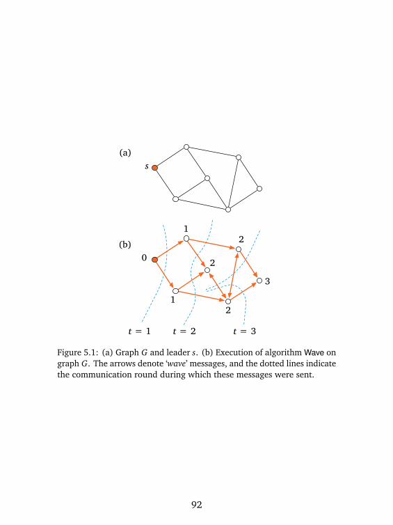
(a)

(b)

s

0

1

1

2

2

2

3

t = 1 t = 2 t = 3

Figure 5.1: (a) Graph G and leader s. (b) Execution of algorithm Wave ongraph G. The arrows denote ‘wave’ messages, and the dotted lines indicatethe communication round during which these messages were sent.

92

to all other ports, switch to state i, and stop; otherwise it does nothing.See Figure 5.1.

The analysis of the algorithm is simple. By induction, all nodes atdistance i from s will receive message ‘wave’ from at least one port inround i, and they will hence output the correct value i. The runningtime of the algorithm is O(diam(G)) rounds in the CONGEST model.

5.5 Breadth-First Search Tree

Algorithm Wave finds the shortest-path distances from a single source s.Now we will do something slightly more demanding: calculate not justthe distances but also the shortest paths.

More precisely, our goal is to construct a breadth-first search tree(BFS tree) T rooted at s. This is a spanning subgraph T = (V, E′) of Gsuch that T is a tree, and for each node v ∈ V , the shortest path from sto v in tree T is also a shortest path from s to v in graph G. We will alsolabel each node v ∈ V with a distance label d(v), so that for each nodev ∈ V we have

d(v) = distT (s, v) = distG(s, v).

See Figure 5.2 for an illustration. We will interpret T as a directed graph,so that each edge is of form (u, v), where d(u)> d(v), that is, the edgespoint towards the root s.

There is a simple centralized algorithm that constructs the BFS treeand distance labels: breadth-first search. We start with an empty treeand unlabeled nodes. First we label the leader s with d(s) = 0. Then instep i = 0,1, . . . , we visit each node u with distance label d(u) = i, andcheck each neighbor v of u. If we have not labeled v yet, we will label itwith d(v) = i + 1, and add the edge (v, u) to the BFS tree. This way allnodes that are at distance i from s in G will be labeled with the distancelabel i, and they will also be at distance i from s in T .

We can implement the same idea as a distributed algorithm in theCONGEST model. We will call this algorithm BFS. In the algorithm,each node v maintains the following variables:

93

(a)

(b)

s

0

1

1

2

2

2

3

Figure 5.2: (a) Graph G and leader s. (b) BFS tree T (arrows) and distancelabels d(v) (numbers).

• d(v): distance to the root.

• p(v): pointer to the parent of node v in tree T (port number).

• C(v): the set of children of node v in tree T (port numbers).

• a(v): acknowledgment—set to 1 when the subtree rooted at v hasbeen constructed.

Here a(v) = 1 denotes a stopping state. When the algorithm stops,variables d(v) will be distance labels, tree T is encoded in variables p(v)and C(v), and all nodes will have a(v) = 1.

Initially, we set d(v)←⊥, p(v)←⊥, C(v)←⊥, and a(v)← 0 foreach node v, except for the root which has d(s) = 0. We will grow treeT from s by iterating the following steps:

• Each node v with d(v) 6= ⊥ and C(v) = ⊥ will send a proposalwith value d(v) to all neighbors.

94

• If a node u with d(u) =⊥ receives some proposals with value j, itwill accept one of them and reject all other proposals. It will setp(u) to point to the node whose proposal it accepted, and it willset d(u)← j + 1.

• Each node v that sent some proposals will set C(v) to be the setof neighbors that accepted proposals.

This way T will grow towards the leaf nodes. Once we reach a leaf node,we will send acknowledgments back towards the root:

• Each node v with a(v) = 1 and p(v) 6=⊥ will send an acknowledg-ment to port p(v).

• Each node v with a(v) = 0 and C(v) 6= ⊥ will set a(v) ← 1when it has received acknowledgments from each port of C(v).In particular, if a node has C(v) =∅, it can set a(v)← 1 withoutwaiting for any acknowledgments.

It is straightforward to verify that the algorithm works correctly andconstructs a BFS tree in O(diam(G)) rounds in the CONGEST model.

Note that the acknowledgments would not be strictly necessary inorder to construct the tree. However, they will be very helpful in thenext section when we use algorithm BFS as a subroutine.

5.6 Leader Election

Algorithm BFS constructs a BFS tree rooted at a single leader, assumingthat we have already elected a leader. Now we will show how to elect aleader. Surprisingly, we can use algorithm BFS to do it!

We will design an algorithm Leader that finds the node with thesmallest identifier; this node will be the leader. The basic idea is verysimple:

(a) We modify algorithm BFS so that we can run multiple copies of itin parallel, with different root nodes. We augment the messages

95

with the identity of the root node, and each node keeps track ofthe variables d, p, C , and a separately for each possible root.

(b) Then we pretend that all nodes are leaders and start running BFS.In essence, we will run n copies of BFS in parallel, and hence wewill construct n BFS trees, one rooted at each node. We will denoteby BFSv the BFS process rooted at node v ∈ V , and we will writeTv for the output of this process.

However, there are two problems: First, it is not yet obvious how all thiswould help with leader election. Second, we cannot implement this ideadirectly in the CONGEST model—nodes would need to send up to ndistinct messages per communication round, one per each BFS process,and there is not enough bandwidth for all those messages.

Fortunately, we can solve both of these issues very easily; see Fig-ure 5.3:

(c) Each node will only send messages related to the tree that hasthe smallest identifier as the root. More precisely, for each node v,let U(v) ⊆ V denote the set of nodes u such that v has receivedmessages related to process BFSu, and let `(v) = min U(v) bethe smallest of these nodes. Then v will ignore messages relatedto process BFSu for all u 6= `(v), and it will only send messagesrelated to process BFS`(v).

We make the following observations:

• In each round, each node will only send messages related to atmost one BFS process. Hence we have solved the second problem—this algorithm can be implemented in the CONGEST model.

• Let s = min V be the node with the smallest identifier. Whenmessages related to BFSs reach a node v, it will set `(v) = s andnever change it again. Hence all nodes will follow process BFSsfrom start to end, and thanks to the acknowledgments, node s willeventually know that we have successfully constructed a BFS treeTs rooted at it.

96

t = 1

t = 2

t = 3

t = 4

73 25 41 6

Figure 5.3: Leader election. Each node v will launch a process BFSv thatattempts to construct a BFS tree Tv rooted at v. Other nodes will happilyfollow BFSv if v is the smallest leader they have seen so far; otherwisethey will start to ignore messages related to BFSv . Eventually, preciselyone of the processes will complete successfully, while all other process willget stuck at some point. In this example, node 1 will be the leader, as ithas the smallest identifier. Process BFS2 will never succeed, as node 1 (aswell as all other nodes that are aware of node 1) will ignore all messagesrelated to BFS2. Node 1 is the only root that will receive acknowledgmentsfrom every child.

97

• Let u 6=min V be any other node. Now there is at least one node, s,that will ignore all messages related to process BFSu. Hence BFSuwill never finish; node u will never receive the acknowledgmentsrelated to tree Tu from all neighbors.

That is, we now have an algorithm with the following properties: afterO(diam(G)) rounds, there is precisely one node s that knows that it isthe unique node s =min V . To finish the leader election process, node swill inform all other nodes that leader election is over; node s will output1 and all other nodes will output 0 and stop.

5.7 All-Pairs Shortest Paths

Now we are ready to design algorithm APSP that solves the all-pairsshortest path problem (APSP) in time O(n).

We already know how to find the shortest-path distances from asingle source; this is efficiently solved with algorithm Wave. Just like wedid with the BFS algorithm, we can also augment Wave with the rootidentifier and hence have a separate process Wavev for each possibleroot v ∈ V . If we could somehow run all these processes in parallel, theneach node would receive a wave from every other node, and hence eachnode would learn the distance to every other node, which is preciselywhat we need to do in the APSP problem. However, it is not obvioushow to achieve a good performance in the CONGEST model:

• If we try to run all Wavev processes simultaneously in parallel, wemay need to send messages related to several waves simultaneouslyover a single edge, and there is not enough bandwidth to do that.

• If we try to run all Wavev processes sequentially, it will take a lotof time: the running time would be O(n diam(G)) instead of O(n).

The solution is to pipeline the Wavev processes so that we can havemany of them running simultaneously in parallel, without congestion.In essence, we want to have multiple wavefronts active simultaneouslyso that they never collide with each other.

98

(a)

(b)

Figure 5.4: (a) BFS tree Ts rooted at s. (b) A depth-first traversal ws of Ts.

To achieve this, we start with the leader election and the constructionof a BFS tree rooted at the leader; let s be the leader, and let Ts be theBFS tree. Then we do a depth-first traversal of Ts. This is a walk ws in Tsthat starts at s, ends at s, and traverses each edge precisely twice; seeFigure 5.4.

More concretely, we move a token along walk ws. We move the tokenslowly: we always spend 2 communication rounds before we move thetoken to an adjacent node. Whenever the token reaches a new node vthat we have not encountered previously during the walk, we launchprocess Wavev . This is sufficient to avoid all congestion!

The key observation here is that the token moves slower than thewaves. The waves move at speed 1 edge per round (along the edgesof G), while the token moves at speed 0.5 edges per round (along theedges of Ts, which is a subgraph of G). This guarantees that two wavesnever collide. To see this, consider two waves Waveu and Wavev , so thatWaveu was launched before Wavev . Let d = distG(u, v). Then it will takeat least 2d rounds to move the token from u to v, but only d roundsfor Waveu to reach node v. Hence Waveu was already past v before we

99

t = 0

t = 1

t = 2

t = 3

t = 4

t = 5

Figure 5.5: Algorithm APSP: the token walks along the BFS tree at speed0.5 (thick arrows), while each Wavev moves along the original graphat speed 1 (dashed lines). The waves are strictly nested: if Wavev wastriggered after Waveu, it will never catch up with Waveu.

triggered Wavev, and Wavev will never catch up with Waveu as both ofthem travel at the same speed. See Figure 5.5 for an illustration.

Hence we have an algorithm APSP that is able to trigger all Wavevprocesses in O(n) time, without collisions, and each of them completesO(diam(G)) rounds after it was launched. Overall, it takes O(n) roundsfor all nodes to learn distances to all other nodes. Finally, the leadercan inform everyone else when it is safe to stop and announce the localoutputs (e.g., with the help of another wave).

5.8 Quiz

Give an example of a graph problem that can be solved in O(1) rounds inthe LOCAL model and cannot be solved in O(n) rounds in the CONGESTmodel. The input has to be an unlabeled graph; that is, the nodes will nothave any inputs (beyond their own degree and their unique identifier).The output can be anything; you are free to construct an artificial graph

100

problem. It is enough to give a brief definition of the graph problem; nofurther explanations are needed.

5.9 Exercises

Exercise 5.1 (prior algorithms). In Chapters 3 and 4 we have seenexamples of algorithms that were designed for the PN and LOCAL models.Many of these algorithms use only small messages—they can be useddirectly in the CONGEST model. Give at least four concrete examples ofsuch algorithms, and prove that they indeed use only small messages.

Exercise 5.2 (edge counting). The edge counting problem is defined asfollows: each node has to output the value |E|, i.e., it has to indicatehow many edges there are in the graph.

Assume that the input graph is connected. Design an algorithmthat solves the edge counting problem in the CONGEST model in timeO(diam(G)).

Exercise 5.3 (detecting bipartite graphs). Assume that the input graphis connected. Design an algorithm that solves the following problem inthe CONGEST model in time O(diam(G)):

• If the input graph is bipartite, all nodes output 1.• Otherwise all nodes output 0.

Exercise 5.4 (detecting complete graphs). We say that a graph G = (V, E)is complete if for all nodes u, v ∈ V , u 6= v, there is an edge u, v ∈ E.

Assume that the input graph is connected. Design an algorithm thatsolves the following problem in the CONGEST model in time O(1):

• If the input graph is a complete graph, all nodes output 1.• Otherwise all nodes output 0.

Exercise 5.5 (gathering). Assume that the input graph is connected. InSection 4.2 we saw how to gather full information on the input graph intime O(diam(G)) in the LOCAL model. Design an algorithm that solvesthe problem in time O(|E|) in the CONGEST model.

101

? Exercise 5.6 (gathering lower bounds). Assume that the input graph isconnected. Prove that there is no algorithm that gathers full informationon the input graph in time O(|V |) in the CONGEST model.

. hint L

? Exercise 5.7 (APSP lower bounds). Assume that the input graph isconnected. Prove that there is no algorithm that solves the APSP problemin time o(|V |) in the CONGEST model.


The name CONGEST is from Peleg’s [36] book. Algorithm APSP is dueto Holzer and Wattenhofer [24]—surprisingly, it was published only asrecently as in 2012.

102

Chapter 6

Randomized Algorithms

All models of computing that we have studied so far were based on theformalism that we introduced in Chapter 3: a distributed algorithm Ais a state machine whose state transitions are determined by functionsinitA,d , sendA,d , and receiveA,d . Everything has been fully deterministic:for a given network and a given input, the algorithm will always producethe same output. In this chapter, we will extend the model so that wecan study randomized distributed algorithms.

6.1 Definitions

Let us first define a randomized distributed algorithms in the PN modelor, in brief, a randomized PN algorithm. We extend the definitions ofSection 3.3 so that the state transitions are chosen randomly accordingto some probability distribution that may depend on the current stateand incoming messages.

More formally, the values of the functions init and receive are discreteprobability distributions over StatesA. The initial state of a node u is arandom variable x0(u) chosen from a discrete probability distribution

initA,d( f (u))

that may depend on the local input f (u). The state at time t is a randomvariable x t(u) chosen from a discrete probability distribution

receiveA,d

x t−1(u), mt(u)

that may depend on the previous state x t−1(u) and on the incomingmessages mt(u). All other parts of the model are as before. In particular,function sendA,d is deterministic.

103

Above we have defined randomized PN algorithms. We can nowextend the definitions in a natural manner to define randomized algo-rithms in the LOCAL model (add unique identifiers) and randomizedalgorithms in the CONGEST model (add unique identifiers and limit thesize of the messages).

6.2 Probabilistic Analysis

In randomized algorithms, performance guarantees are typically proba-bilistic. For example, we may claim that algorithm A stops in time T withprobability p.

Note that all probabilities here are over the random choices in thestate transitions. We do not assume that our network or the local inputsare chosen randomly; we still require that the algorithm performs wellwith worst-case inputs. For example, if we claim that algorithm A solvesproblem Π on graph family F in time T (n) with probability p, then wecan take any graph G ∈ F and any port-numbered network N with G asits underlying graph, and we guarantee that with probability at least pthe execution of A in N stops in time T (n) and produces a correct outputg ∈ Π(G); as usual, n is the number of nodes in the network.

We may occasionally want to emphasize the distinction between“Monte Carlo” and “Las Vegas” type algorithms:

• Monte Carlo: Algorithm A always stops in time T (n); the outputis a correct solution to problem Π with probability p.

• Las Vegas: Algorithm A stops in time T (n)with probability p; whenit stops, the output is always a correct solution to problem Π.

However, Monte Carlo algorithms are not as useful in the field of dis-tributed computing as they are in the context of classical centralizedalgorithms. In centralized algorithms, we can usually take a Monte Carloalgorithm and just run it repeatedly until it produces a feasible solution;hence we can turn a Monte Carlo algorithm into a Las Vegas algorithm.This is not necessarily the case with distributed algorithms: verifying

104

the output of an algorithm may require global information on the entireoutput, and gathering such information may take a long time. In thischapter, we will mainly focus on Las Vegas algorithms, i.e., algorithmsthat are always correct but may occasionally be slow, but in the exerciseswe will also encounter Monte Carlo algorithms.

6.3 With High Probability

We will use the word failure to refer to the event that the algorithm didnot meet its guarantees—in the case of a Las Vegas algorithm, it did notstop in time T (n), and in the case of Monte Carlo algorithms, it did notproduce a correct output. The word success refers to the opposite case.

Usually we want to show that the probability of a failure is negligible.In computer science, we are usually interested in asymptotic analysis,and hence in the context of randomized algorithms, it is convenient ifwe can show that the success probability approaches 1 when n increases.Even better, we would like to let the user of the algorithm choose howquickly the success probability approaches 1.

This idea is captured in the phrase “with high probability” (commonlyabbreviated w.h.p.). Please note that this phrase is not a vague subjectivestatement but it carries a precise mathematical meaning: it refers to thesuccess probability of 1−1/nc , where we can choose any constant c > 0.(Unfortunately, different sources use slightly different definitions; forexample, it may also refer to the success probability of 1−O(1)/nc forany constant c > 0.)

In our context, we say that algorithm A solves problem Π on graphfamily F in time O(T (n)) with high probability if the following holds:

• I can choose any constant c > 0. Algorithm A may depend on thisconstant.

• Then if I run A in any network N that has its underlying graphin F , the algorithm will stop in time O(T (n)) with probability atleast 1− 1/nc , and the output is a feasible solution to problem Π.

105

Note that the O(·) notation in the running time is used to hide thedependence on c. This is a crucial point. For example, it would not makemuch sense to say that the running time is at most log n with probability1− 1/nc for any constant c > 0. However, it is perfectly reasonable tosay that the running time is, e.g., at most c log n or 2c log n or simplyO(log n) with probability 1− 1/nc for any constant c > 0.

6.4 Randomized Coloring in Bounded-DegreeGraphs

In Chapter 4 we presented a deterministic algorithm that finds a (∆+ 1)-coloring in a graph of maximum degree∆. In this section, we will designa randomized algorithm that solves the same problem. The running timesare different:

• the deterministic algorithm runs in O(∆+ log∗ n) rounds.• the randomized algorithm runs in O(log n) rounds with high prob-

ability.

Hence for large values of ∆, the randomized algorithm can be muchfaster.

6.4.1 Algorithm Idea

A running time of O(log n) is very typical for a randomized distributedalgorithm. Often randomized algorithms follow the strategy that in eachstep each node picks a value randomly from some probability distribution.If the value conflicts with the values of the neighbors, the node will tryagain next time; otherwise the node outputs the current value and stops.If we can prove that each node stops in each round with a constantprobability, we can prove that after Θ(log n) all nodes have stoppedw.h.p. This is precisely what we saw in the analysis of the randomizedpath-coloring algorithm in Section 1.5.

However, adapting the same strategy to graphs of maximum degree∆ requires some thought. If each node just repeatedly tries to pick a

106

random color from 1, 2, . . . ,∆+1, the success probability may be fairlylow for large values of ∆.

Therefore we will adopt a strategy in which nodes are slightly lessaggressive. Nodes will first randomly choose whether they are active orpassive in this round; each node is passive with probability 1/2. Onlyactive nodes will try to pick a random color among those colors that arenot yet used by their neighbors.

Informally, the reason why this works well is the following. Assumethat we have a node v with d neighbors that have not yet stopped. Thenthere are at least d + 1 colors among which v can choose whenever it isactive. If all of the d neighbors were also active and if they happened topick distinct colors, we would have only a

1d + 1

chance of picking a color that is not used by any of the neighbors. How-ever, in our algorithm on average only d/2 neighbors are active. If wehave at most d/2 active neighbors, we will succeed in picking a freecolor with probability at least

d + 1− d/2d + 1

>12

,

regardless of what the active neighbors do.

6.4.2 Algorithm

Let us now formalize the algorithm. For each node u, let

C(u) = 1, 2, . . . , degG(u) + 1

be the color palette of the node; node u will output one of the colors ofC(u).

In the algorithm, node u maintains the following variables:

• State s(u) ∈ 0, 1

107

• Color c(u) ∈ ⊥ ∪ C(u).

Initially, s(u)← 1 and c(u)←⊥. When s(u) = 1 and c(u) 6= ⊥, node ustops and outputs color c(u).

In each round, node u always sends c(u) to each port. The incomingmessages are processed as follows, depending on the current state of thenode:

• s(u) = 1 and c(u) 6=⊥:

– This is a stopping state; ignore incoming messages.

• s(u) = 1 and c(u) =⊥:

– Let M(u) be the set of messages received.

– Let F(u) = C(u) \M(u) be the set of free colors.– With probability 1/2, set c(u)←⊥; otherwise choose a c(u) ∈

F(u) uniformly at random.

– Set s(u)← 0.

• s(u) = 0:

– Let M(u) be the set of messages received.

– If c(u) ∈ M(u), set c(u)←⊥.

– Set s(u)← 1.

Informally, the algorithm proceeds as follows. For each node u, itsstate s(u) alternates between 1 and 0:

• When s(u) = 1, the node either decides to be passive and setsc(u) = ⊥, or it decides to be active and picks a random colorc(u) ∈ F(u). Here F(u) is the set of colors that are not yet used byany of the neighbors that are stopped.

• When s(u) = 0, the node verifies its choice. If the current color c(u)conflicts with one of the neighbors, we go back to the initial states(u)← 1 and c(u)←⊥. However, if we were lucky and managedto pick a color that does not conflict with any of our neighbors, wekeep the current value of c(u) and switch to the stopping state.

108

6.4.3 Analysis

It is easy to see that if the algorithm stops, then the output is a proper(∆+ 1)-coloring of the underlying graph. Let us now analyze how longit takes for the nodes to stop.

In the analysis, we will write st(u) and ct(u) for values of variabless(u) and c(u) after round t = 0, 1, . . . , and Mt(u) and Ft(u) for the valuesof M(u) and F(u) during round t = 1,2, . . . . We also write

Kt(u) =

v ∈ V : u, v ∈ E, st−1(v) = 1, ct−1(v) =⊥

for the set of competitors of node u during round t = 1,3,5, . . . ; theseare the neighbors of u that have not yet stopped.

First, let us prove that with probability at least 1/4, a running nodesucceeds in picking a color that does not conflict with any of its neighbors.

Lemma 6.1. Fix a node u ∈ V and time t = 1,3,5, . . . . Assume thatst−1(u) = 1 and ct−1(u) =⊥, i.e., u has not stopped before round t. Thenwith probability at least 1/4, we have st+1(u) = 1 and ct+1(u) 6=⊥, i.e., uwill stop after round t + 1.

Proof. Let f = |Ft(u)| be the number of free colors during round t, andlet k = |Kt(u)| be the number of competitors during round t. Note thatf ≥ k + 1, as the size of the palette is one larger than the number ofneighbors.

Let us first study the case that u is active. As we have got f freecolors, for any given color x ∈ N we have

Pr

ct(u) = x

ct(u) 6=⊥

≤ 1/ f .

In particular, this holds for any color x = ct(v) chosen by any activecompetitor v ∈ Kt(u):

Pr

ct(u) = ct(v)

ct(u) 6=⊥, ct(v) 6=⊥

≤ 1/ f .

That is, we conflict with an active competitor with probability at most1/ f . Naturally, we cannot conflict with a passive competitor:

Pr

ct(u) = ct(v)

ct(u) 6=⊥, ct(v) =⊥

= 0.

109

As a competitor is active with probability

Pr

ct(v) 6=⊥

= 1/2,

and the random variables ct(u) and ct(v) are independent, the probabilitythat we conflict with a given competitor v ∈ Kt(u) is

Pr

ct(u) = ct(v)

ct(u) 6=⊥

≤1

2 f.

By the union bound, the probability that we conflict with some competitoris

Pr

ct(u) = ct(v) for some v ∈ Kt(u)

ct(u) 6=⊥

≤k

2 f,

which is less than 1/2 for all k ≥ 0 and all f ≥ k + 1. Put otherwise,node u will avoid conflicts with probability

Pr

ct(u) 6= ct(v) for all v ∈ Kt(u)

ct(u) 6=⊥

>12

.

So far we have studied the conditional probabilities assuming that uis active. This happens with probability

Pr

ct(u) 6=⊥

= 1/2.

Therefore node u will stop after round t + 1 with probability

Pr

ct+1(u) 6=⊥] =

Pr

ct(u) 6=⊥ and ct(u) 6= ct(v) for all v ∈ Kt(u)]> 1/4.

Now we can continue with the same argument as what we used inSection 1.5 to analyze the running time. Fix a constant c > 0. Define

T (n) = 2(c + 1) log4/3 n.

We will prove that the algorithm stops in T(n) rounds. First, let usconsider an individual node. Note the exponent c + 1 instead of c in thestatement of the lemma; this will be helpful later.

110

Lemma 6.2. Fix a node u ∈ V . The probability that u has not stoppedafter T (n) rounds is at most 1/nc+1.

Proof. By Lemma 6.1, if node u has not stopped after round 2i, it willstop after round 2i+2 with probability at least 1/4. Hence the probabilitythat it has not stopped after T (n) rounds is at most

(3/4)T (n)/2 =1

(4/3)(c+1) log4/3 n=

1nc+1

.

Now we are ready to analyze the time until all nodes stop.

Theorem 6.3. The probability that all nodes have stopped after T(n)rounds is at least 1− 1/nc .

Proof. Follows from Lemma 6.2 by the union bound.

Note that T(n) = O(log n) for any constant c. Hence we concludethat the algorithm stops in O(log n) rounds with high probability, andwhen it stops, it outputs a vertex coloring with ∆+ 1 colors.

6.5 Quiz

Consider a cycle with 10 nodes, and label the nodes with a randompermutation of the numbers 1, 2, . . . , 10 (uniformly at random). A nodeis a local maximum if its label is larger than the labels of its two neighbors.Let X be the number of local maxima. What is the expected value of X?

6.6 Exercises

Exercise 6.1 (larger palette). Assume that we have a graph without anyisolated nodes. We will design a graph-coloring algorithm A that is a biteasier to understand and analyze than the algorithm of Section 6.4. Inalgorithm A, each node u proceeds as follows until it stops:

• Node u picks a color c(u) from 1, 2, . . . , 2d uniformly at random;here d is the degree of node u.

111

• Node u compares its value c(u) with the values of all neighbors. Ifc(u) is different from the values of its neighbors, u outputs c(u)and stops.

Present this algorithm in a formally precise manner, using the state-machine formalism. Analyze the algorithm, and prove that it finds a2∆-coloring in time O(log n) with high probability.

Exercise 6.2 (unique identifiers). Design a randomized PN algorithm Athat solves the following problem in O(1) rounds:

• As input, all nodes get value |V |.• Algorithm outputs a labeling f : V → 1,2, . . . ,χ for some χ =|V |O(1).

• With high probability, f (u) 6= f (v) for all nodes u 6= v.

Analyze your algorithm and prove that it indeed solves the problemcorrectly.

In essence, algorithm A demonstrates that we can use randomnessto construct unique identifiers, assuming that we have some informationon the size of the network. Hence we can take any algorithm B designedfor the LOCAL model, and combine it with algorithm A to obtain a PNalgorithm B′ that solves the same problem as B (with high probability).

. hint M

Exercise 6.3 (large independent sets). Design a randomized PN al-gorithm A with the following guarantee: in any graph G = (V, E) ofmaximum degree ∆, algorithm A outputs an independent set I such thatthe expected size of the I is |V |/O(∆). The running time of the algorithmshould be O(1). You can assume that all nodes know ∆.

. hint N

Exercise 6.4 (max cut problem). Let G = (V, E) be a graph. A cutis a function f : V → 0,1. An edge u, v ∈ E is a cut edge in fif f (u) 6= f (v). The size of cut f is the number of cut edges, and amaximum cut is a cut of the largest possible size.

112

(a) Prove: If G = (V, E) is a bipartite graph, then a maximum cut has|E| edges.

(b) Prove: If G = (V, E) has a cut with |E| edges, then G is bipartite.

(c) Prove: For any α > 1/2, there exists a graph G = (V, E) in whichthe maximum cut has fewer than α|E| edges.

. hint O

Exercise 6.5 (max cut algorithm). Design a randomized PN algorithmA with the following guarantee: in any graph G = (V, E), algorithm Aoutputs a cut f such that the expected size of cut f is at least |E|/2. Therunning time of the algorithm should be O(1).

Note that the analysis of algorithm A also implies that for any graphthere exists a cut with at least |E|/2.

. hint P

Exercise 6.6 (maximal independent sets). Design a randomized PNalgorithm that finds a maximal independent set in time O(∆+ log n)with high probability.

. hint Q

? Exercise 6.7 (maximal independent sets quickly). Design a random-ized distributed algorithm that finds a maximal independent set in timeO(log n) with high probability.

. hint R


Algorithm of Section 6.4 and the algorithm of Exercise 6.1 are fromBarenboim and Elkin’s book [7, Section 10.1].

113

Part IV

Proving Impossibility Results

114

Chapter 7

Covering Maps

Chapters 3–6 have focused on positive results; now we will turn ourattention to techniques that can be used to prove negative results. Wewill start with so-called covering maps—we will use covering maps toprove that many problems cannot be solved at all with deterministicPN-algorithms.

7.1 Definition

A covering map is a topological concept that finds applications in manyareas of mathematics, including graph theory. We will focus on onespecial case: covering maps between port-numbered networks.

Let N = (V, P, p) and N ′ = (V ′, P ′, p′) be port-numbered networks,and let φ : V → V ′. We say that φ is a covering map from N to N ′ if thefollowing holds:

(a) φ is a surjection: φ(V ) = V ′.

(b) φ preserves degrees: degN (v) = degN ′(φ(v)) for all v ∈ V .

(c) φ preserves connections and port numbers: p(u, i) = (v, j)implies p′(φ(u), i) = (φ(v), j).

See Figures 7.1–7.3 for examples.We can also consider labeled networks, for example, networks with

local inputs. Let f : V → X and f ′ : V ′→ X . We say that φ is a coveringmap from (N , f ) to (N ′, f ′) if φ is a covering map from N to N ′ and thefollowing holds:

(d) φ preserves labels: f (v) = f ′(φ(v)) for all v ∈ V .

115

N:

N’:

a1, 3a1, 2a1, 1

b1, 1b1, 2

c1, 1c1, 2

d1, 1

a2, 3a2, 2a2, 1

b2, 1b2, 2

c2, 1c2, 2

d2, 1

a, 3a, 2a, 1

b, 1b, 2

c, 1c, 2

d, 1

Figure 7.1: There is a covering map φ from N to N ′ that maps ai 7→ a,bi 7→ b, ci 7→ c, and di 7→ d for each i ∈ 1, 2.

116

N:

N’:

v1, 1v1, 2

v3, 1v3, 2

v2, 1v2, 2

v, 1v, 2

Figure 7.2: There is a covering map φ from N to N ′ that maps vi 7→ v foreach i ∈ 1,2,3. Here N is a simple port-numbered network but N ′ isnot.

N:

N’: v, 1

v1, 1 v2, 1

Figure 7.3: There is a covering map φ from N to N ′ that maps vi 7→ v foreach i ∈ 1,2. Again, N is a simple port-numbered network but N ′ isnot.

117

7.2 Covers and Executions

Now we will study covering maps from the perspective of deterministicPN-algorithms. The basic idea is that a covering map φ from N to N ′

fools any PN-algorithm A: a node v in N is indistinguishable from thenode φ(v) in N ′.

Without further ado, we state the main result and prove it—manyapplications and examples will follow.

Theorem 7.1. Assume that

(a) A is a deterministic PN-algorithm with X = InputA,

(b) N = (V, P, p) and N ′ = (V ′, P ′, p′) are port-numbered networks,

(c) f : V → X and f ′ : V ′→ X are arbitrary functions, and

(d) φ : V → V ′ is a covering map from (N , f ) to (N ′, f ′).

Let

(e) x0, x1, . . . be the execution of A on (N , f ), and

(f) x ′0, x ′1, . . . be the execution of A on (N ′, f ′).

Then for each t = 0,1, . . . and each v ∈ V we have x t(v) = x ′t(φ(v)).

Proof. We will use the notation of Section 3.3.2; the symbols with aprime refer to the execution of A on (N ′, f ′). In particular, m′t(u

′, i) isthe message received by u′ ∈ V ′ from port i in round t in the executionof A on (N ′, f ′), and m′t(u

′) is the vector of messages received by u′.The proof is by induction on t. To prove the base case t = 0, let

v ∈ V , d = degN (v), and v′ = φ(v); we have

x ′0(v′) = initA,d( f

′(v′)) = initA,d( f (v)) = x0(v).

For the inductive step, let (u, i) ∈ P, (v, j) = p(u, i), d = degN (u),` = degN (v), u′ = φ(u), and v′ = φ(v). Let us first consider the messagessent by v and v′; by the inductive assumption, these are equal:

sendA,`(x′t−1(v

′)) = sendA,`(x t−1(v)).

118

A covering map φ preserves connections and port numbers: (u, i) =p(v, j) implies (u′, i) = p′(v′, j). Hence mt(u, i) is component j ofsendA,`(x t−1(v)), and m′t(u

′, i) is component j of sendA,`(x ′t−1(v′)). It

follows that mt(u, i) = m′t(u′, i) and mt(u) = m′t(u

′). Therefore

x ′t(u′) = receiveA,d

x ′t−1(u′), m′t(u

′)

= receiveA,d

x t−1(u), mt(u)

= x t(u).

In particular, if the execution of A on (N , f ) stops in time T , the exe-cution of A on (N ′, f ′) stops in time T as well, and vice versa. Moreover,φ preserves the local outputs: xT (v) = x ′T (φ(v)) for all v ∈ V .

7.3 Examples

We will give representative examples of negative results that we can easilyderive from Theorem 7.1. First, we will observe that a deterministicPN-algorithm cannot break symmetry in a cycle—unless we providesome symmetry-breaking information in local inputs.

Lemma 7.2. Let G = (V, E) be a cycle graph, let A be a deterministicPN-algorithm, and let f be a constant function f : V → 0. Then there isa simple port-numbered network N = (V, P, p) such that

(a) the underlying graph of N is G, and

(b) if A stops on (N , f ), the output is a constant function g : V → cfor some c.

Proof. Label the nodes V = v1, v2, . . . , vn along the cycle so that theedges are

E =

v1, v2, v2, v3, . . . , vn−1, vn, vn, v1

.

Choose the port numbering p as follows:

p : (v1, 1) 7→ (v2, 2), (v2, 1) 7→ (v3, 2), . . . ,

(vn−1, 1) 7→ (vn, 2), (vn, 1) 7→ (v1, 2).

119

See Figure 7.2 for an illustration in the case n= 3.Define another port-numbered network N ′ = (V ′, P ′, p′) with V ′ =

v, P ′ = (v, 1), (v, 2), and p(v, 1) = (v, 2). Let f ′ : V ′→ 0. Define afunction φ : V → V ′ by setting φ(vi) = v for each i.

Now we can verify that φ is a covering map from (N , f ) to (N ′, f ′).Assume that A stops on (N , f ) and produces an output g. By Theorem 7.1,A also stops on (N ′, f ′) and produces an output g ′. Let c = g ′(v). Now

g(vi) = g ′(φ(vi)) = g ′(v) = c

for all i.

In the above proof, we never assumed that the execution of A onN ′ makes any sense—after all, N ′ is not even a simple port-numberednetwork, and there is no underlying graph. Algorithm A was neverdesigned to be applied to such a strange network with only one node.Nevertheless, the execution of A on N ′ is formally well-defined, andTheorem 7.1 holds. We do not really care what A outputs on N ′, but theexistence of a covering map can be used to prove that the output of Aon N has certain properties. It may be best to interpret the executionof A on N ′ as a thought experiment, not as something that we wouldactually try to do in practice.

Lemma 7.2 has many immediate corollaries.

Corollary 7.3. Let F be the family of cycle graphs. Then there is nodeterministic PN-algorithm that solves any of the following problems onF :

(a) maximal independent set,(b) 1.999-approximation of a minimum vertex cover,(c) 2.999-approximation of a minimum dominating set,(d) maximal matching,(e) vertex coloring,(f) weak coloring,(g) edge coloring.

120

Proof. In each of these cases, there is a graph G ∈ F such that a constantfunction is not a feasible solution in the network N that we constructedin Lemma 7.2.

For example, consider the case of dominating sets; other cases aresimilar. Assume that G = (V, E) is a cycle with 3k nodes. Then aminimum dominating set consists of k nodes—it is sufficient to take everythird node. Hence a 2.999-approximation of a minimum dominatingset consists of at most 2.999k < 3k nodes. A solution D = V violatesthe approximation guarantee, as D has too many nodes, while D =∅ isnot a dominating set. Hence if A outputs a constant function, it cannotproduce a 2.999-approximation of a minimum dominating set.

Lemma 7.4. There is no deterministic PN-algorithm that finds a weakcoloring for every 3-regular graph.

Proof. Again, we are going to apply the standard technique: pick asuitable 3-regular graph G, find a port-numbered network N that has Gas its underlying graph, find a smaller network N ′ such that we have acovering map φ from N to N ′, and apply Theorem 7.1.

However, it is not immediately obvious which 3-regular graph wouldbe appropriate; hence we try the simplest possible case first. Let G =(V, E) be the complete graph on four nodes: V = s, t, u, v , and we havean edge between any pair of nodes; see Figure 7.4. The graph is certainly3-regular: each node is adjacent to the other three nodes.

Now it is easy to verify that the edges of G can be partitioned intoa 2-factor X and a 1-factor Y . The 2-factor consists of a cycle and a1-factor consists of disjoint edges. We can use the factors to guide theselection of port numbers in N .

In the cycle induced by X , we can choose symmetric port numbersusing the same idea as what we had in the proof of Lemma 7.2; one endof each edge is connected to port 1 while the other end is connected toport 2. For the edges of the 1-factor Y , we can assign port number 3 ateach end. We have constructed the port-numbered network N that isillustrated in Figure 7.4.

121

XY

YX

Xs

X

t

uv

N:

N’:

s, 3s, 2s, 1

v, 3v, 2v, 1

u, 3u, 2u, 1

t, 3t, 2t, 1

G:

x, 3x, 2x, 1

Figure 7.4: Graph G is the complete graph on four nodes. The edges of Gcan be partitioned into a 2-factor X and a 1-factor Y . Network N has Gas its underlying graph, and there is a covering map φ from N to N ′

122

Now we can verify that there is a covering mapφ from N to N ′, whereN ′ is the network with one node illustrated in Figure 7.4. Thereforein any algorithm A, if we do not have any local inputs, all nodes of Nwill produce the same output. However, a constant output is not a weakcoloring of G.

In the above proof, we could have also partitioned the edges of Ginto three 1-factors, and we could have used the 1-factorization to guidethe selection of port numbers. However, the above technique is moregeneral: there are 3-regular graphs that do not admit a 1-factorizationbut that can be partitioned into a 1-factor and a 2-factor.

So far we have used only one covering map in our proofs; the fol-lowing lemma gives an example of the use of more than one coveringmap.

Lemma 7.5. Let F = G3, G4 , where G3 is the cycle graph with 3 nodes,and G4 is the cycle graph with 4 nodes. There is no deterministic PN-algorithm that solves the following problem Π on F : in Π(G3) all nodesoutput 3 and in Π(G4) all nodes output 4.

Proof. We again apply the construction of Lemma 7.2; for each i ∈3,4, let Ni be the symmetric port-numbered network that has Gi asthe underlying graph.

Now it would be convenient if we could construct a covering mapfrom N4 to N3; however, this is not possible (see the exercises). Thereforewe proceed as follows. Construct a one-node network N ′ as in theproof of Lemma 7.2, construct the covering map φ3 from N3 to N ′, andconstruct the covering map φ4 from N4 to N ′; see Figure 7.5. The localinputs are assumed to be all zeros.

Let A be a PN-algorithm, and let c be the output of the only node ofN ′. If we apply Theorem 7.1 to φ3, we conclude that all nodes of N3output c; if A solves Π on G3, we must have c = 3. However, if we applyTheorem 7.1 to φ4, we learn that all nodes of N4 also output c = 3, andhence A cannot solve Π on F .

123

N’:

N3: N4:

φ3 φ4

Figure 7.5: The structure of the proof of Lemma 7.5.

We have learned that a deterministic PN-algorithm cannot determinethe length of a cycle. In particular, a deterministic PN-algorithm cannotdetermine if the underlying graph is bipartite.

7.4 Quiz

Let G = (V, E) be a graph. A set X ⊆ V is a k-tuple dominating set iffor every v ∈ V we have |ballG(v, 1)∩ X | ≥ k. Consider the problem offinding a minimum 2-tuple dominating set in cycles. What is the best(i.e. smallest) approximation ratio we can achieve in the PN model?

7.5 Exercises

We use the following definition in the exercises. A graph G is homoge-neous if there are port-numbered networks N and N ′ and a coveringmap φ from N to N ′ such that N is simple, the underlying graph of N isG, and N ′ has only one node. For example, Lemma 7.2 shows that allcycle graphs are homogeneous.

124

Exercise 7.1 (finding port numbers). Consider the graph G and networkN ′ illustrated in Figure 7.6. Find a simple port-numbered network Nsuch that N has G as the underlying graph and there is a covering mapfrom N to N ′.

Exercise 7.2 (homogeneity). Assume that G is homogeneous and itcontains a node of degree at least two. Give several examples of graphproblems that cannot be solved with any deterministic PN-algorithm inany family of graphs that contains G.

Exercise 7.3 (regular and homogeneous). Show that the followinggraphs are homogeneous:

(a) graph G illustrated in Figure 7.7,

(b) graph G illustrated in Figure 7.6.

. hint S

Exercise 7.4 (complete graphs). Recall that we say that a graph G =(V, E) is complete if for all nodes u, v ∈ V , u 6= v, there is an edgeu, v ∈ E. Show that

(a) any 2k-regular graph is homogeneous,

(b) any complete graph with 2k nodes has a 1-factorization,

(c) any complete graph is homogeneous.

Exercise 7.5 (dominating sets). Let ∆ ∈ 2,3, . . . , let ε > 0, and letF consist of all graphs of maximum degree at most ∆. Show that it ispossible to find a (∆+1)-approximation of a minimum dominating set inconstant time in family F with a deterministic PN-algorithm. Show thatit is not possible to find a (∆+1−ε)-approximation with a deterministicPN-algorithm.

. hint T

Exercise 7.6 (covers with covers). What is the connection betweencovering maps and the vertex cover 3-approximation algorithm in Sec-tion 3.6?

125

b, 3b, 2b, 1

c, 3c, 2c, 1

d, 3d, 2d, 1

a, 3a, 2a, 1

N’:

G:

Figure 7.6: Graph G and network N ′ for Exercises 7.1 and 7.3b.

Figure 7.7: Graph G for Exercise 7.3a.

126

Figure 7.8: Graph G for Exercise 7.7.

? Exercise 7.7 (3-regular and not homogeneous). Consider the graphG illustrated in Figure 7.8.

(a) Show that G is not homogeneous.

(b) Present a deterministic PN-algorithm A with the following prop-erty: if N is a simple port-numbered network that has G as theunderlying graph, and we execute A on N , then A stops and pro-duces an output where at least one node outputs 0 and at leastone node outputs 1.

(c) Find a simple port-numbered network N that has G as the under-lying graph, a port-numbered network N ′, and a covering mapφ from N to N ′ such that N ′ has the smallest possible number ofnodes.

. hint U

? Exercise 7.8 (covers and connectivity). Assume that N = (V, P, p) andN ′ = (V ′, P ′, p′) are simple port-numbered networks such that there is acovering map φ from N to N ′. Let G be the underlying graph of networkN , and let G′ be the underlying graph of network N ′.

(a) Is it possible that G is connected and G′ is not connected?

(b) Is it possible that G is not connected and G′ is connected?

? Exercise 7.9 (k-fold covers). Let N = (V, P, p) and N ′ = (V ′, P ′, p′) besimple port-numbered networks such that the underlying graphs of Nand N ′ are connected, and assume that φ : V → V ′ is a covering map

127

from N to N ′. Prove that there exists a positive integer k such thatthe following holds: |V | = k|V ′| and for each node v′ ∈ V ′ we have|φ−1(v′)| = k. Show that the claim does not necessarily hold if theunderlying graphs are not connected.


The use of covering maps in the context of distributed algorithm wasintroduced by Angluin [3]. The general idea of Exercise 7.7 can be tracedback to Yamashita and Kameda [42], while the specific construction inFigure 7.8 is from Bondy and Murty’s textbook [9, Figure 5.10]. Parts ofexercises 7.1, 7.3, 7.4, and 7.5 are inspired by our work [4,39].

128

Chapter 8

Local Neighborhoods

Covering maps can be used to argue that a given problem cannot besolved at all with deterministic PN algorithms. Now we will study theconcept of locality, which can be used to argue that a given problemcannot be solved fast, in any model of distributed computing.

8.1 Definitions

Let N = (V, P, p) and N ′ = (V ′, P ′, p′) be simple port-numbered networks,with the underlying graphs G = (V, E) and G′ = (V ′, E′). Fix the localinputs f : V → Y and f ′ : V ′ → Y , a pair of nodes v ∈ V and v′ ∈ V ′,and a radius r ∈ N. Define the radius-r neighborhoods

U = ballG(v, r), U ′ = ballG′(v′, r).

We say that (N , f , v) and (N ′, f ′, v′) have isomorphic radius-r neighbor-hoods if there is a bijection ψ: U → U ′ with ψ(v) = v′ such that

(a) ψ preserves degrees: degN (v) = degN ′(ψ(v)) for all v ∈ U .

(b) ψ preserves connections and port numbers: p(u, i) = (v, j) if andonly if p′(ψ(u), i) = (ψ(v), j) for all u, v ∈ U .

(c) ψ preserves local inputs: f (v) = f ′(ψ(v)) for all v ∈ U .

The function ψ is called an r-neighborhood isomorphism from (N , f , v)to (N ′, f ′, v′). See Figure 8.1 for an example.

8.2 Local Neighborhoods and Executions

Theorem 8.1. Assume that

129

u v

Figure 8.1: Nodes u and v have isomorphic radius-2 neighborhoods,provided that we choose the port numbers appropriately. Therefore in anyalgorithm A the state of u equals the state of v at time t = 0, 1, 2. However,at time t = 3, 4, . . . this does not necessarily hold.

(a) A is a deterministic PN algorithm with X = InputA,

(b) N = (V, P, p) and N ′ = (V ′, P ′, p′) are simple port-numberednetworks,

(c) f : V → X and f ′ : V ′→ X are arbitrary functions,

(d) v ∈ V and v′ ∈ V ′,

(e) (N , f , v) and (N ′, f ′, v′) have isomorphic radius-r neighborhoods.

Let

(f) x0, x1, . . . be the execution of A on (N , f ), and

(g) x ′0, x ′1, . . . be the execution of A on (N ′, f ′).

Then for each t = 0,1, . . . , r we have x t(v) = x ′t(v′).

Proof. Let G and G′ be the underlying graphs of N and N ′, respectively.We will prove the following stronger claim by induction: for each t =0,1, . . . , r, we have x t(u) = x ′t(ψ(u)) for all u ∈ ballG(v, r − t).

To prove the base case t = 0, let u ∈ ballG(v, r), d = degN (u), andu′ =ψ(u); we have

x ′0(u′) = initA,d( f

′(u′)) = initA,d( f (u)) = x0(u).

For the inductive step, assume that t ≥ 1 and

u ∈ ballG(v, r − t).

130

Let u′ =ψ(u). By inductive assumption, we have

x ′t−1(u′) = x t−1(u).

Now consider a port (u, i) ∈ P. Let (s, j) = p(u, i). We have s, u ∈ E,and therefore

distG(s, v)≤ distG(s, u) + distG(u, v)≤ 1+ r − t.

Define s′ =ψ(s). By inductive assumption we have

x ′t−1(s′) = x t−1(s).

The neighborhood isomorphism ψ preserves the port numbers: (s′, j) =p′(u′, i). Hence all of the following are equal:

(a) the message sent by s to port j on round t,(b) the message sent by s′ to port j on round t,(c) the message received by u from port i on round t,(d) the message received by u′ from port i on round t.

As the same holds for any port of u, we conclude that

x ′t(u′) = x t(u).

To apply Theorem 8.1 in the LOCAL model, we need to includeunique identifiers in the local inputs f and f ′.

8.3 Example: 2-Coloring Paths

We know from Chapter 1 that one can find a proper 3-coloring of a pathvery fast, in O(log∗ n) rounds. Now we will show that 2-coloring is muchharder; it requires linear time.

To reach a contradiction, suppose that there is a deterministic dis-tributed algorithm A that finds a proper 2-coloring of any path graphin o(n) rounds in the LOCAL model. Then there has to be a number n0

131

such that for any number of nodes n≥ n0, the running time of algorithmA is at most (n− 3)/2. Pick some integer k ≥ n0/2, and consider twopaths: path G contains 2k nodes, with unique identifiers 1,2, . . . , 2k,and path H contains 2k+ 1 nodes, with unique identifiers

1,2, . . . , k, 2k+ 1, k+ 1, k+ 2, . . . , 2k.

Here is an example for k = 3:

21 64 53

21 57 43 6

G:

H:

We assign the port numbers so that for all degree-2 nodes port number1 points towards node 1:

21 64 53

21 57 43 6

G:

H:

1 1 2 1 2 1 2 1 2 1

2 1 2 1 2 1 2 1 2 11 1

By assumption, the running time of A is at most

(n− 3)/2≤ (2k+ 1− 3)/2= k− 1

rounds in both cases. Since node 1 has got the same radius-(k− 1)neighborhood in G and H, algorithm A will produce the same output fornode 1 in both networks:

21 64 53

21 57 43 6

G:

H:

1 1 2 1 2 1 2 1 2 1

2 1 2 1 2 1 2 1 2 11 1

By a similar reasoning, node 2k (i.e., the last node of the path) also hasto produce the same output in both cases:

132

21 64 53

21 57 43 6

G:

H:

1 1 2 1 2 1 2 1 2 1

2 1 2 1 2 1 2 1 2 11 1

However, now we reach a contradiction. In path H, in any proper 2-coloring nodes 1 and 2k have the same color—for example, both of themare of color 1, as shown in the following picture:

21 22 11 1H:

If algorithm A works correctly, it follows that nodes 1 and 2k mustproduce the same output in path H. However, then it follows that nodes1 and 2k produces the same output also in G, too, but this cannot happenin any proper 2-coloring of G.

?1 1? ??

21 22 11 1

G:

H:

We conclude that algorithm A fails to find a proper 2-coloring in at leastone of these instances.

8.4 Quiz

The caption of Figure 8.1 says: “However, at time t = 3,4, . . . thisdoes not necessarily hold.” Design some deterministic algorithm A thatdemonstrates this for the PN model. When you run algorithm A in thenetwork of Figure 8.1, the following should happen:

• At time t = 0,1, 2, nodes u and v have the same local state.• At time t = 3,4, . . . , nodes u and v have different local states.

Please try to design your algorithm so that its behavior does not dependon the choice of the port numbering: for each node x and each timestep t, the state of x has to be the same regardless of how you choose theport numbers. A short, informal description of the algorithm is enough.

133

8.5 Exercises

Exercise 8.1 (edge coloring). In this exercise, the graph family F con-sists of path graphs.

(a) Show that it is possible to find a 2-edge coloring in time O(n) withdeterministic PN-algorithms.

(b) Show that it is not possible to find a 2-edge coloring in time o(n)with deterministic PN-algorithms.

(c) Show that it is not possible to find a 2-edge coloring in time o(n)with deterministic LOCAL-algorithms.

Exercise 8.2 (maximal matching). In this exercise, the graph family Fconsists of path graphs.

(a) Show that it is possible to find a maximal matching in time O(n)with deterministic PN-algorithms.

(b) Show that it is not possible to find a maximal matching in timeo(n) with deterministic PN-algorithms.

(c) Show that it is possible to find a maximal matching in time o(n)with deterministic LOCAL-algorithms.

Exercise 8.3 (optimization). In this exercise, the graph familyF consistsof path graphs. Can we solve the following problems with deterministicPN-algorithms? If yes, how fast? Can we solve them any faster in theLOCAL model?

(a) Minimum vertex cover.

(b) Minimum dominating set.

(c) Minimum edge dominating set.

Exercise 8.4 (approximation). In this exercise, the graph family Fconsists of path graphs. Can we solve the following problems withdeterministic PN-algorithms? If yes, how fast? Can we solve them anyfaster in the LOCAL model?

134

(a) 2-approximation of a minimum vertex cover?

(b) 2-approximation of a minimum dominating set?

Exercise 8.5 (auxiliary information). In this exercise, the graph familyF consists of path graphs, and we are given a 4-coloring as input. Weconsider deterministic PN-algorithms.

(a) Show that it is possible to find a 3-coloring in time 1.

(b) Show that it is not possible to find a 3-coloring in time 0.

(c) Show that it is possible to find a 2-coloring in time O(n).

(d) Show that it is not possible to find a 2-coloring in time o(n).

? Exercise 8.6 (orientations). In this exercise, the graph family Fconsists of cycle graphs, and we are given some orientation as input. Thetask is to find a consistent orientation, i.e., an orientation such that boththe indegree and the outdegree of each node is 1.

(a) Show that this problem cannot be solved with any deterministicPN-algorithm.

(b) Show that this problem cannot be solved with any deterministicLOCAL-algorithm in time o(n).

(c) Show that this problem can be solved with a deterministic PN-algorithm if we give n as input to all nodes. How fast? Prove tightupper and lower bounds on the running time.

? Exercise 8.7 (local indistinguishability). Consider the graphs G1and G2 illustrated in Figure 8.2. Assume that A is a deterministic PN-algorithm with running time 2. Show that A cannot distinguish betweennodes v1 and v2. That is, there are simple port-numbered networks N1and N2 such that Ni has Gi as the underlying graph, and the output ofv1 in N1 equals the output of v2 in N2.

. hint V

135

v1 v2

G1 G2

Figure 8.2: Graphs for Exercise 8.7.


Local neighborhoods were used to prove negative results in the contextof distributed computing by, e.g., Linial [30].

136

Chapter 9

Round Elimination

In this chapter we introduce the basic idea of a proof technique, calledround elimination. Round elimination is based on the following idea.Assume that there exists a distributed algorithm S0 with complexityT solving a problem Π0. Then there exists a distributed algorithm S1with complexity T − 1 for solving another problem Π1. That is, if wecan solve problem Π0 in T communication rounds, then we can solvea related problem Π1 exactly one round faster—we can “eliminate oneround”. If this operation is repeated T times, we end up with somealgorithm ST with round complexity 0 for some problem ΠT . If ΠT isnot a trivial problem, that is, cannot be solved in 0 rounds, we havereached a contradiction: therefore the assumption that Π0 can be solvedin T rounds has to be wrong. This is a very useful approach, as it ismuch easier to reason about 0-round algorithms than about algorithmsin general.

9.1 Bipartite Model and Biregular Trees

When dealing with round elimination, we will consider a model that is avariant of the PN model from Chapter 3. We will restrict our attentionto specific families of graphs (see Figure 9.1):

(a) Bipartite. The set of nodes V is partitioned into two sets: theactive nodes VA and the passive nodes VP . The partitioning forms aproper 2-coloring of the graph, i.e., each edge connects an activenode with a passive node. The role of a node—active or passive—is part of the local input.

(b) Biregular trees. We will assume that the input graphs are biregulartrees: the graph is connected, there are no cycles, each node in

137

(a)

(b)

Figure 9.1: The bipartite model; black nodes are active and white nodesare passive. (a) A (3, 3)-biregular tree. (b) A (3, 2)-biregular tree.

VA has degree d or 1, and each node in VP has degree δ or 1.We say that such a tree is (d,δ)-biregular. See Figure 9.1 for anillustration.

9.1.1 Bipartite Locally Verifiable Problem

We consider a specific family of problems, called bipartite locally verifiableproblems. Such a problem is defined as a 3-tuple Π= (Σ,A,P), where:

• Σ is a finite alphabet.

• A and P are finite collections of multisets, where each multisetA ∈ A and P ∈ P consists of a finite number of elements from Σ.These are called the active and passive configurations.

138

Recall that multisets are sets that allow elements to be repeated. We usethe notation [x1, x2, . . . , xk] for a multiset that contains k elements; forexample, [1,1, 2,2, 2] is a multiset with two 1s and three 2s. Note thatthe order of elements does not matter, for example, [1, 1, 2] = [1, 2, 1] =[2,1, 1].

In problem Π, each active node v ∈ VA must label its incident deg(v)edges with elements of Σ such that the labels of the incident edges,considered as a multiset, form an element of A. The order of the labelsdoes not matter. The passive nodes do not have outputs. Instead, werequire that for each passive node the labels of its incident edges, againconsidered as a multiset, form an element of P. A labeling ϕ : E→ Σ isa solution to Π if and only if the incident edges of all active and passivenodes are labeled according to some configuration.

In this chapter we will only consider labelings such that all nodes ofdegree 1 accept any configuration: these will not be explicitly mentionedin what follows. Since we only consider problems in (d,δ)-biregulartrees, each active configuration will have d elements and each passiveconfiguration δ elements.

9.1.2 Examples

To illustrate the definition of bipartite locally verifiable labelings, weconsider some examples (see Figure 9.2).

Edge Coloring. A c-edge coloring is an assignment of labels from1, 2, . . . , c to the edges such that no node has two incident edges withthe same label.

Consider the problem of 5-edge coloring (3, 3)-biregular trees. Thealphabet Σ consists of the five edge colors 1,2,3,4,5. The activeconfigurations consist of all multisets of three elements [x , y, z], suchthat all elements are distinct and come fromΣ. The problem is symmetric,and the passive configurations consist of the same multisets:

A= P=

[1,2, 3], [1, 2,4], [1,2, 5], [1,3, 4], [1, 3,5],

[1,4, 5], [2, 3,4], [2,3, 5], [2,4, 5], [3, 4,5]

.

139

3 2

452

13 1

2

12

35 2

3

1 4

43

P P

PMU

UP P

P

MU

MU M

U

P M

PM

OI

IOO

OI O

O

OI

OI O

I

O O

OI

11

2

2

22

2 23

3

3 1

31

1

1

1

1 1

1

1

33

(a)

(b)

(c)

(d)

Figure 9.2: Bipartite locally verifiable labeling problems. (a) 5-edgecoloring in a (3,3)-biregular tree. (b) Maximal matching in a (3,3)-biregular tree. (c) Sinkless orientation in a (3, 3)-biregular tree. (d) Weak3-labeling in a (3,2)-biregular tree.

140

Maximal Matching. A maximal matching M is a subset of the edgessuch that no two incident edges are in M and no edge can be addedto M .

Consider maximal matching on (3,3)-biregular trees. To encodea matching, we could use just two labels: M for matched and U forunmatched. Such a labeling, however, has no way of guaranteeingmaximality. We use a third label P, called a pointer:

Σ= M,P,U.

The active nodes either output [M,U,U], denoting that the edge markedM is in the matching, or they output [P,P,P], denoting that they areunmatched, and thus all passive neighbors must be matched with anotheractive node:

A=

[M,U,U], [P,P,P]

.

Passive nodes must verify that they are matched with at most one node,and that if they have an incident label P, then they also have an incidentlabel M (to ensure maximality). Hence the passive configurations are

P=

[M,P,P], [M,P,U], [M,U,U], [U,U,U]

.

Sinkless Orientation. A sinkless orientation is an orientation of theedges such that each node has an edge oriented away from it. That is,no node is a sink. We will consider here sinkless orientation in (3,3)-biregular trees; leaf nodes can be sinks, but nodes of degree 3 must haveat least one outgoing edge.

To encode sinkless orientation, each active node chooses an orienta-tion of its incident edges: outgoing edges are labeled O and incomingedges I. Thus the alphabet is Σ = O, I. Each node must have an outgo-ing edge, so the active configurations are all multisets that contain atleast one O:

A=

[O, x , y]

x , y ∈ Σ

.

The passive configurations are similar, but the roles of the labels arereversed: an outgoing edge for an active node is an incoming edge for a

141

passive node. Therefore each passive node requires that at least one ofits incident edges is labeled I, and the passive configurations are

P=

[I, x , y]

x , y ∈ Σ

.

Weak Labeling. We will use the following problem as the example inthe remainder of this chapter. Consider (3,2)-biregular trees. A weak3-labeling is an assignment of labels from the set 1,2,3 to the edgessuch that each active node has at least two incident edges labeled withdifferent labels. Each passive node must have its incident edges labeledwith the same label. The problem can be formalized as

Σ= 1,2, 3,

A=

[1,1, 2], [1, 1,3], [1, 2,2], [1,2, 3], [1, 3,3], [2,2, 3], [2,3, 3]

,

P=

[1,1], [2,2], [3, 3]

.

9.2 Introducing Round Elimination

Round elimination is based on the following basic idea. Assume thatwe can solve some bipartite locally verifiable problem Π0 in T commu-nication rounds on (d,δ)-biregular trees. Then there exists a bipartitelocally verifiable problem Π1, called the output problem of Π0, that canbe solved in T − 1 rounds on (δ, d)-biregular trees. The output problemis uniquely defined, and we refer to the output problem of Π as re(Π).The definition of output problem will be given in Section 9.2.2.

A single round elimination step is formalized in the following lemma.

Lemma 9.1 (Round elimination lemma). Let Π be bipartite locally ver-ifiable problem that can be solved in T rounds in (d,δ)-biregular trees.Then the output problem re(Π) of Π can be solved in T − 1 rounds in(δ, d)-biregular trees.

142

9.2.1 Impossibility Using Iterated Round Elimination

Lemma 9.1 can be iterated, applying it to the output problem of theprevious step. This will yield a sequence of T + 1 problems

Π0→ Π1→ ·· · → ΠT ,

where Πi+1 = re(Πi) for each i = 0, 1, . . . , T − 1.If we assume that there is a T -round algorithm for Π0, then by an

iterated application of Lemma 9.1, there is a (T − 1)-round algorithmfor Π1, a (T − 2)-round algorithm for Π2, and so on. In particular, thereis a 0-round algorithm for ΠT .

Algorithms that run in 0 rounds are much easier to reason aboutthan algorithms in general. Since there is no communication, each activenode must simply map its input, essentially its degree, to some output.In particular, we can try to show that there is no 0-round algorithmfor ΠT . If this is the case, we have a contradiction with our originalassumption: there is no T -round algorithm for Π0.

We will now proceed to formally define output problems.

9.2.2 Output Problems

For each locally verifiable problem Π we will define a unique outputproblem re(Π).

Let Π0 = (Σ0,A0,P0) be a bipartite locally verifiable problem on(d,δ)-biregular trees. We define the output problem Π1 = re(Π0) =(Σ1,A1,P1) of Π0 on (δ, d)-biregular trees as follows—note that weswapped the degrees of active vs. passive nodes here.

The alphabetΣ1 consists of all possible non-empty subsets ofΣ0. Theroles of the active and passive nodes are inverted, and new configurationsare computed as follows.

(a) The active configurations A1 consist of all multisets

[X1, X2, . . . , Xδ], where X i ∈ Σ1 for all i = 1, . . . ,δ,

such that for every choice of x1 ∈ X1, x2 ∈ X2, . . . , xδ ∈ Xδ wehave [x1, x2, . . . , xδ] ∈ P0, i.e., it is a passive configuration of Π0.

143

(b) The passive configurations P1 consist of all multisets

[Y1, Y2, . . . , Yd], where Yi ∈ Σ1 for all i = 1, . . . , d,

for which there exists a choice y1 ∈ Y1, y2 ∈ Y2, . . . , yd ∈ Yd with[y1, y2, . . . , yd] ∈ A0, i.e., it is an active configuration of Π0.

9.2.3 Example: Weak 3-labeling

To illustrate the definition, let us construct the output problem re(Π0) =(Σ1,A1,P1) of weak 3-labeling problem Π0 = (Σ0,A0,P0). Recall that

Σ0 = 1,2, 3,

A0 =

[1,1, 2], [1, 1,3], [1,2, 2], [1,2, 3], [1, 3,3], [2,2, 3], [2, 3,3]

,

P0 =

[1,1], [2,2], [3, 3]

.

The alphabet Σ1 consists of all possible (non-empty) subsets of Σ0:

Σ1 =

1, 2, 3, 1, 2, 1, 3, 2,3, 1,2, 3

.

The active configurations A1 are all multisets [X , Y ] with X , Y ∈ Σ1such that all choices of elements x ∈ X and y ∈ Y result in a multiset[x , y] ∈ P0. For example X = 1 and Y = 1,2 is not a valid choice:we could choose x = 1 and y = 2 to construct [1,2] /∈ P0. In general,whenever |X |> 1 or |Y |> 1, we can find x ∈ X , y ∈ Y with x 6= y , andthen [x , y] /∈ P0. Therefore the only possibilities are |X |= |Y |= 1, andthen we must also have X = Y . We obtain

A1 =¦

1, 1

,

2, 2

,

3, 3

©

.

But since the active configurations only allow singleton sets, we canrestrict ourselves to them when listing the possible passive configurations;we obtain simply

P1 =¦

1, 1, 2

,

1, 1, 3

,

1, 2, 2

,

1, 2, 3

,

1, 3, 3

,

2, 2, 3

,

2, 3, 3

©

.

144

9.2.4 Complexity of Output Problems

In this section we prove Lemma 9.1 that states that the output problemre(Π) of Π can be solved one round faster than Π.

The proof is by showing that we can truncate the execution of aT -round algorithm and output the set of possible outputs. As we will see,this is a solution to the output problem.

Proof of Lemma 9.1. Assume that we can solve some problem Π0 =(Σ0,A0,P0) on (d,δ)-biregular trees in T rounds using some determin-istic PN-algorithm S. We want to design an algorithm that works in(δ, d)-biregular trees and solves Π1 = re(Π0) in T − 1 rounds.

Note that we are considering the same family of networks, but weare only switching the sides that are marked as active and passive. Wewill call these Π0-active and Π1-active sides, respectively.

The algorithm for solving Π1 works as follows. Let N = (V, P, p) beany port-numbered network with a (δ, d)-biregular tree as the underlyinggraph. Each Π1-active node u, in T − 1 rounds, gathers its full (T − 1)-neighborhood ballN (u, T − 1). Now it considers all possible outputs ofits Π0-active neighbors under the algorithm S, and outputs these.

Formally, this is done as follows. When N is a port-numbered net-work, we use ballN (u, r) to refer to the information within distance rfrom node u, including the local inputs of the nodes in this region, as wellas the port numbers of the edges connecting nodes within this region.We say that a port-numbered network H is compatible with ballN (u, r) ifthere is a node v ∈ H such that ballH(v, r) is isomorphic to ballN (u, r).

For each neighbor v of u, node u constructs all possible fragmentsballH(v, T) such that H is compatible with ballN (u, T − 1) and has a(δ, d)-biregular tree as its underlying graph. Then u simulates the Π0-algorithm S on ballH(v, T). The algorithm outputs some label x ∈ Σ0on the edge u, v. Node u adds each such label x to set S(u, v); finallynode u will label edge u, v with S(u, v).

By construction, S(u, v) is a nonempty set of labels from Σ0, i.e.,S(u, v) ∈ Σ1. We now prove that the sets S(u, v) form a solution to Π1.We use the assumption that the underlying graph G is a tree. Let H be

145

121 231

23

2

1

1

23

1 2

1

232

1 2

12

3

1

1 2 32

1

1

2

23

1

1 2 32

1

123

1 2 2 31

12

231

1

22

3

12

1

12 3

21

3

1

2

v u wball(v, 4)

ball(u, 3)

ball(w, 4)

Figure 9.3: Illustration of the round elimination step. A fragment of a(2,3)-biregular tree. The 3-neighborhood of node u consists of the grayarea. The 4-neighborhoods of nodes v and w consist of the blue andorange areas, respectively. Since the input is a tree, these intersect exactlyin the 3-neighborhood of u.

any port-numbered network compatible with ballN (u, T − 1). Considerany two neighbors v and w of u: since there are no cycles, we have

ballH(v, T )∩ ballH(w, T ) = ballH(u, T − 1) = ballN (u, T − 1).

In particular, once ballH(u, T − 1) is fixed, the outputs of v and w, re-spectively, depend on the structures of ballH(v, T ) \ ballH(u, T − 1) andballH(w, T) \ ballH(u, T − 1), which are completely distinct. See Fig-ure 9.3 for an illustration. Therefore, if there exist x ∈ S(u, v) andy ∈ S(u, w), then there exists a port-numbered network H such thatrunning S, node v outputs x on v, u and node w outputs y on w, u.This further implies that since S is assumed to work correctly on all port-numbered networks, for any combination of x1 ∈ S(u, v1), x2 ∈ S(u, v2),. . . , xδ ∈ S(u, vδ), we must have that

[x1, x2, . . . , xδ] ∈ P0.

146

This implies that

[S(u, v1), S(u, v2), . . . , S(u, vδ)] ∈ A1.

It remains to show that for each Π0-active node v, it holds that thesets S(u1, v), S(u2, v), . . . , S(ud , v), where ui are neighbors of v, form aconfiguration in P1. To see this, note that theΠ1-active nodes ui simulateS on every port-numbered fragment, including the true neighborhoodballN (v, T) of v. This implies that the output of v on v, ui runningS in network N is included in S(ui , v). Since S is assumed to be acorrect algorithm, these true outputs x1 ∈ S(u1, v), x2 ∈ S(u2, v), . . . ,xd ∈ S(ud , v) form a configuration

[x1, x2, . . . , xd] ∈ A0,

which implies that

[S(u1, v), S(u2, v), . . . , S(ud , v)] ∈ P1,

as required.

9.2.5 Example: Complexity of Weak 3-labeling

Now we will apply the round elimination technique to show that theweak 3-labeling problem is not solvable in 1 round. To do this, we showthat the output problem of weak 3-labeling is not solvable in 0 rounds.

Lemma 9.2. Weak 3-labeling is not solvable in 1 round in the PN-modelon (3,2)-biregular trees.

Proof. In Section 9.2.3 we saw the output problem of weak 3-labeling.We will now show that this problem is not solvable in 0 rounds on (2, 3)-biregular trees. By Lemma 9.1, weak 3-labeling is then not solvable in 1round on (3, 2)-biregular trees. Let Π1 = (Σ1,A1,P1) denote the outputproblem of weak 3-labeling.

147

In a 0-round algorithm an active node v sees only its own side (activeor passive) and its own port numbers. Since

A1 =¦

1, 1

,

2, 2

,

3, 3

©

,

each active node v must output the same label X ∈

1, 2, 3

onboth of its incident edges.

Since all active nodes look the same, they all label their incidentedges with exactly one label X . Since [X , X , X ] is not in P1 for anyX ∈ Σ1, we have proven the claim.

9.2.6 Example: Iterated Round Elimination

We will finish this chapter by applying round elimination twice to weak3-labeling. We will see that the problem

Π2 = re(Π1) = re(re(Π0))

obtained this way is 0-round solvable.Let us first construct Π2. Note that this is again a problem on (3, 2)-

biregular trees. We first simplify notation slightly; the labels ofΠ1 are setsand labels ofΠ2 would be sets of sets, which gets awkward to write down.But the configurations in Π1 only used singleton sets. Therefore we canleave out all non-singleton sets without changing the problem, and thenwe can rename each singleton set x to x . After these simplifications,we have got

Σ1 = 1,2, 3,

A1 =

[1,1], [2,2], [3, 3]

,

P1 =

[1,1, 2], [1, 1,3], [1,2, 2], [1,2, 3], [1, 3,3], [2,2, 3], [2, 3,3]

.

Alphabet Σ2 consists of all non-empty subsets of Σ1, that is

Σ2 =

1, 2, 3, 1, 2, 1, 3, 2,3, 1,2, 3

.

148

The active configurations are all multisets [X1, X2, X3]where X1, X2, X3 ∈Σ2 such that any way of choosing x1 ∈ X1, x2 ∈ X2, and x3 ∈ X3 isa configuration in P1. There are many cases to check, the followingobservation will help here (the proof is left as Exercise 9.4):

• P1 consists of all 3-element multisets over Σ1 where at least oneof the elements is not 1, at least one of the elements is not 2, andat least one of the elements is not 3.

• It follows that A2 consists of all 3-element multisets over Σ2 whereat least one of the elements does not contain 1, at least one of theelements does not contain 2, and at least one of the elements doesnot contain 3.

It follows that we can enumerate all possible configurations e.g. asfollows (here X , Y, Z ∈ Σ2):

A2 =¦

X , Y, Z

X ⊆ 1, 2, Y ⊆ 1, 3, Z ⊆ 2, 3©

∪¦

X , Y, Z

X ⊆ 1, Y ⊆ 2, 3, Z ⊆ 1,2, 3©

∪¦

X , Y, Z

X ⊆ 2, Y ⊆ 1, 3, Z ⊆ 1,2, 3©

∪¦

X , Y, Z

X ⊆ 3, Y ⊆ 1, 2, Z ⊆ 1,2, 3©

.

(9.1)

On the passive side, P2 consists of all multisets [X , Y ] where we canchoose x ∈ X and y ∈ Y with [x , y] ∈ A1. But [x , y] ∈ A1 is equivalentto x = y, and hence P2 consists of all multisets [X , Y ] where we canchoose some x ∈ X and choose the same value x ∈ Y . Put otherwise,

P2 =¦

X , Y

X ∈ Σ2, Y ∈ Σ2, X ∩ Y 6=∅©

.

Lemma 9.3. Let Π0 denote the weak 3-labeling problem. The problemΠ2 = re(re(Π0)) = (Σ2,A2,P2) is solvable in 0 rounds.

Proof. The active nodes always choose the configuration

1,2, 1,3, 2,3

∈ A2

149

and assign the sets in some way using the port numbers, e.g., the edgeincident to port 1 is labeled with 2,3, the edge incident to port 2 islabeled with 1, 3, and the edge incident to port 3 is labeled with 1, 2.

Since each pair of these sets has a non-empty intersection, no matterwhich sets are assigned to the incident edges of passive nodes, theseform a valid passive configuration in P2.

9.3 Quiz

Consider the following bipartite locally verifiable labeling problem Π=(Σ,A,P) on (2, 2)-biregular trees:

Σ= 1,2, 3,4, 5,6,

A=

[1,6], [2, 5], [3, 4]

, and

P=

[x , y]

x ∈ 3,5, 6, y ∈ 1,2, 3,4, 5,6

∪

[x , y]

x ∈ 4,5, 6, y ∈ 2,3, 4,5, 6

.

Give a 0-round algorithm for solving Π.

9.4 Exercises

Exercise 9.1 (encoding graph problems). Even if a graph problem isdefined for general (not bipartite) graphs, we can often represent it inthe bipartite formalism. If we take a d-regular tree G and subdivideeach edge, we arrive at a (d, 2)-biregular tree H, where the active nodesrepresent the nodes of G and passive nodes represent the edges of G.

Use this idea to encode the following graph problems as bipartitelocally verifiable labelings in (d, 2)-biregular trees. Give a brief expla-nation of why your encoding is equivalent to the original problem. Youcan ignore the leaf nodes and their constraints; it is sufficient to spec-ify constraints for the active nodes of degree d and passive nodes ofdegree 2.

(a) Vertex coloring with d + 1 colors.

150

(b) Maximal matching.(c) Dominating set.(d) Minimal dominating set.

Exercise 9.2 (algorithms in the bipartite model). The bipartite modelcan be used to run algorithms from the standard PN and LOCAL models.Using the idea of Exercise 9.1, we encode the maximal independent setproblem in 3-regular trees as the following bipartite locally verifiableproblem Π= (Σ,A,P) in (3,2)-biregular trees:

Σ= I,O,P,

A=

[I, I, I], [P,O,O]

,

P=

[I,P], [I,O], [O,O]

.

In A, the first configuration corresponds to a node in the independentset X , and the second configuration to a node not in X . A node not in Xpoints to a neighboring active node with the label P: the node pointed tohas to be in X . The passive configurations ensure that two active nodesconnected by a passive node are not both in X , and that the pointer Palways points to a node in X .

Assume that the active nodes are given a 4-coloring c as input. That is,c : VA→ 1, 2, 3, 4 satisfies c(v) 6= c(u) whenever the active nodes v, u ∈VA share a passive neighbor w ∈ VP . The nodes also know whether theyare active or passive, but the nodes do not have any other information.

Present a PN-algorithm in the state machine formalism for solving Π.Prove that your algorithm is correct. What is its running time? Howdoes it compare to the complexity of solving maximal independent setin the PN model, given a 4-coloring?

Exercise 9.3 (Round Eliminator). There is a computer program, calledRound Eliminator, that implements the round elimination technique andthat you can try out in a web browser:

https://github.com/olidennis/round-eliminator

151


Let Π0 be the weak 3-labeling problem defined in Section 9.1.2. Use theRound Eliminator to find out what are Π1 = re(Π0) and Π2 = re(Π1).In your answer you need to show how to encode Π0 in a format that issuitable for the Round Eliminator, what were the answers you got fromthe Round Eliminator, and how to turn the answers back into our usualmathematical formalism.

Exercise 9.4 (iterated round elimination). Fill in the missing detailsin Section 9.2.6 to show that formula (9.1) is a correct definition ofthe active configurations for problem Π2 (i.e., it contains all possibleconfigurations and only them).

Exercise 9.5 (solving weak 3-labeling). Present a 2-round deterministicPN-algorithm for solving weak 3-labeling in (3,2)-biregular trees.

Exercise 9.6 (sinkless orientation). Consider the sinkless orientationproblem, denoted by Π, on (3,3)-biregular trees from Section 9.1.2.Compute the output problems re(Π) and re(re(Π)); include a justificationfor your results.


Linial’s [30] lower bound for vertex coloring in cycles already used aproof technique that is similar to round elimination. However, for along time it was thought that this is an ad-hoc technique that is onlyapplicable to this specific problem. This started to change in 2016, whenthe same idea found another very different application [11]. Roundelimination as a general-purpose technique was defined and formalizedby Brandt [10] in 2019, and implemented as a computer program byOlivetti [34].

152

Chapter 10

Sinkless Orientation

In this chapter we will study the complexity of sinkless orientation, aproblem that was introduced in the previous chapter. This is a problemthat is understood well: we will design algorithms and show that theseare asymptotically optimal.

Recall that sinkless orientation is the problem of orienting the edgesof the tree so that each internal node has got at least one outgoing edge.We begin by studying sinkless orientation on paths (or (2,2)-biregulartrees), and show that we can easily argue about local neighborhoods toprove a tight lower bound result. However, when we switch to (3,3)-biregular trees, we will need the round elimination technique to do thesame.

10.1 Sinkless Orientation on Paths

We define sinkless orientation on paths to be the following bipartite locallyverifiable problem Π = (Σ,A,P). The alphabet is Σ = I,O, with theinterpretation that I indicates that the edge is oriented towards the activenode (“incoming”) and O indicates that the edge is oriented away fromthe active node (“outgoing”). Each active node must label at least oneincident edge with O, and thus the active configurations are

A=

[O, I], [O,O]

.

Each passive node must have at least one incident edge labeled with I,and thus the passive configurations are

P=

[I,O], [I, I]

.

As previously, nodes of degree 1 are unconstrained; the edges incidentto them can be labeled arbitrarily.

153

Figure 10.1: Propagation of a sinkless orientation on paths. Orienting asingle edge (orange) forces the orientation of the path all the way to theother endpoint.

10.1.1 Hardness of Sinkless Orientation

We begin by showing that solving sinkless orientation requires Ω(n)rounds on (2,2)-biregular trees.

Lemma 10.1. Solving sinkless orientation on (2, 2)-biregular trees in thebipartite PN-model requires at least n/4−1 rounds, even if the nodes knowthe value n.

Let us first see why the lemma is intuitively true. Consider a path,as illustrated in Figure 10.1. Each active node u must choose somelabel for its incident edges, and at least one of these labels must be O.Then its passive neighbor v over the edge labeled with O must have itsother incident edge labeled I. This further implies that the other activeneighbor w of v must label its other edge with O. The original output ofu propagates through the path and the outputs of other nodes far awayfrom u depend on the output of u.

Let us now formalize this intuition.

Proof of Lemma 10.1. Consider any algorithm A running in T (n) = o(n)rounds. Then there exists n0 such that for all n ≥ n0, we have thatT(n) ≤ (n− 5)/4. Now fix such an integer n and let T = T(n) denotethe running time of the algorithm.

Consider an active node v in the middle of a path N on n nodes. LetballN (v, T ) denote the T -neighborhood of v. Assume that ballN (v, T ) isconsistently port-numbered from left to right, as illustrated in Figure 10.2.Node v must use the output label O on one of its incident edges; withoutloss of generality, assume that this is port 1. We can now construct acounterexample N ′ as follows. Take two copies of ballN (v, T ), denotedby ballN ′(v1, T) and ballN ′(v2, T). In particular, this includes the port-numbering in ballN (v, T). Add one new node that is connected to the

154

1 1 1 1 1 1 1 1 12 2 2 2 2 2 2 2 2

1 1 1 1 1 1 1 1 12 2 2 2 2 2 2 2 2

1 1 1 1 1 1 1 1 12 2 2 2 2 2 2 2 2

v OI

v1 OI

v2 OI

Figure 10.2: Sinkless orientation lower bound. Assume T = 4. Top: anyalgorithm must fix some output labeling with an outgoing edge for a fixedneighborhood ballN (v, 4). Bottom: Copying the same 4-neighborhoodtwice, and arranging the copies towards the same node creates an inputN ′ where the two nodes orient towards the middle. There is no legal wayto label the rest of the path.

right endpoint of both ballN ′(v1, T ) and ballN ′(v2, T ). Finally, add leavesat the other endpoints of ballN ′(v1, T ) and ballN ′(v2, T ); see Figure 10.2for an illustration. We claim that the algorithm A fails on N ′.

By definition, edges must be labeled alternatively O and I startingfrom both v1 and v2. Therefore we must eventually find an active nodelabeled [I, I] or a passive node labeled [O,O], an incorrect solution.

The total number of nodes in N ′ is n = 2(2T + 1) + 3 = 4T + 5,giving T = (n− 5)/4. Thus solving sinkless orientation requires at leastT + 1= (n− 5)/4+ 1≥ n/4− 1 rounds, as required.

10.1.2 Solving Sinkless Orientation on Paths

The proof of Lemma 10.1 shows that it is impossible to solve sinklessorientation on paths in sublinear number of rounds. Now we will showa linear upper bound: it is possible to solve sinkless orientation once allnodes see an endpoint of the path.

Lemma 10.2. Sinkless orientation can be solved in bn/2c rounds in thebipartite PN-model on (2,2)-biregular trees.

155

Proof. The idea of the algorithm is the following: initially send messagesfrom the leaves towards the middle of the path. Orient edges againstthe incoming messages, i.e., toward the closest leaf. Once the messagesreach the midpoint of the path, all edges have been correctly orientedaway from the midpoint.

The algorithm works as follows. Initially all non-leaf nodes wait.The leaf nodes send a message to their neighbor and stop. If they areactive, they output I on their incident edge. Whenever a node receives amessage for the first time, in the next round it sends a message to theother port and stops. If it is an active node, it outputs O in the portfrom which it received the message, and I in the other port. That is, itorients its incident edges towards the closer leaf. If a node receives twomessages in the same round, it is the midpoint of the path; it does notsend any further messages. If it is an active node, it outputs O on bothof its incident edges.

The algorithm runs in bn/2c rounds: on paths with an even numberof nodes, all nodes have received a message in round n/2− 1, and thusstop in the next round. On paths with an odd number of nodes, themiddle node receives two messages in round bn/2c and stops.

It remains to show that our algorithm is correct. All leaf nodesare trivially labeled correctly. Any active non-leaf node always has anincident label O. Now consider a passive node u: there is an active vthat sends u a message before stopping. This node will output I on u, v,and thus u is also correctly labeled.

Theorem 10.3. The complexity of sinkless orientation on paths is Θ(n).

Proof. Follows from Lemmas 10.1 and 10.2.

10.2 Sinkless Orientation on Trees

In Section 10.1 we saw that if we require that degree-2 nodes have atleast one outgoing edge, we arrive at a problem that is hard already inthe case of paths. The proof of hardness was a straightforward argumentthat used local neighborhoods.

156

However, what happens if we relax the problem slightly and allowany orientation around degree-2 nodes? The proof of hardness fromSection 10.1.1 no longer works, but does the problem get easier to solve?

For concreteness, let us consider trees of maximum degree 3, that is,both active and passive nodes have degree at most 3; the case of higherdegrees is very similar. We define the problem so that nodes of degree1 and 2 are unconstrained, but nodes of degree 3 must have at leastone outgoing edge. We can encode it as follows as a bipartite locallyverifiable problem Π0 = (Σ0,A0,P0):

Σ0 = O, I,

A0 =

[O], [I], [O,O], [O, I], [I, I], [O, I, I], [O,O, I], [O,O,O]

,

P0 =

[O], [I], [O,O], [O, I], [I, I], [I,O,O], [I, I,O], [I, I, I]

.

Here we have listed all possible configurations for nodes of degrees 1, 2,and 3.

10.2.1 Solving Sinkless Orientation on Trees

The algorithm for solving sinkless orientation on trees uses ideas similarto the algorithm on paths: each node u must determine the closestunconstrained node v, i.e., a node of degree 1 or 2, and the path fromu to v is oriented away from u. This will make all nodes happy: eachactive node of degree 3 has an outgoing edge, and all other nodes areunconstrained.

Let us call nodes of degree 1 and 2 special nodes. We must be carefulin how the nodes choose the special node: the algorithm would fail iftwo nodes want to orient the same edge in different directions.

The algorithm functions as follows. In the first round, only specialnodes are sending messages, broadcasting to each port. Then the specialnodes stop and, if they are active nodes, they output I on each edge.Nodes of degree 3 wake up in the first round in which they receive at leastone message. In the next round they broadcast to each port from whichthey did not receive a message in the previous round. After sending

157

this message, the nodes stop. If they are active nodes, they orient theirincident edges towards the smallest port from which they received amessage: output O on that edge, and I on the other edges.

Correctness. Assume that the closest special nodes are at distancet from some node u. Assume that v is one of those nodes, and let(v1, v2, . . . , vt+1) denote the unique path from v = v1 to u = vt+1. Weclaim that in each round i, node vi broadcasts to vi+1. By assumption, vis also one of the closest special nodes to all vi; otherwise there wouldbe a closer special node to u as well. In particular, there will never bea broadcast from vi+1 to vi, as then vi+1 would have a different closerspecial node. Therefore each vi will broadcast to vi+1 in round i. Thisimplies that in round t, node u will receive a broadcast from vt .

All nodes that receive a broadcast become happy: Active nodesoutput O on one of the edges from which they received a broadcast,making them happy. They output I on the other edges, so each passivenode is guaranteed that every edge from which it receives a broadcasthas the label I.

Time Complexity. It remains to bound the round by which all nodeshave received a broadcast. To do this, we observe that each node is atdistance O(log n) from a special node.

Consider a fragment of a 3-regular tree centered around some node v,and assume that there are no special nodes near v. Then at distance 1from v there are 3 nodes, at distance 2 there are 6 nodes, at distance 3there are 12 nodes, and so on. In general, if we do not have any specialnodes within distance i, then at distance i there are 3 · 2i−1 > 2i nodesin the tree. At distance i = log2 n, we would have more than n nodes.Thus, within distance log2 n, there has to be a special node. Since eachnode can stop once it has received a broadcast, the running time of thealgorithm is O(log n).

158

10.2.2 Roadmap: Next Steps

We have seen that sinkless orientation in trees can be solved in O(log n)rounds. We would like to now prove a matching lower bound andshow that sinkless orientation cannot be solved in o(log n) rounds. Wewill apply the round elimination technique from Chapter 9 to do this.However, we will need one further refinement to the round eliminationtechnique that will make our life a lot easier: we can ignore all non-maximal configurations. We will explain this idea in detail in Section 10.3,and then we are ready to prove the hardness result in Section 10.4.

10.3 Maximal Output Problems

In Chapter 9 we saw how to use the round elimination technique toconstruct the output problem Π′ = re(Π) for any given bipartite locallyverifiable problem Π. We will now make an observation that allowsus to simplify the description of output problems. We will change thedefinition of output problems to include this simplification.

Consider an output problem Π′ = (Σ,A,P). Recall that Σ now con-sists of sets of labels. Assume that there are two configurations

X = [X1, X2, . . . , Xd],

Y = [Y1, Y2, . . . , Yd],

in A. We say that Y contains X if we have X i ⊆ Yi for all i.If Y contains X , then configuration X is redundant; whenever an

algorithm solving Π′ would like to use the configuration X , it can equallywell use Y instead:

• Active nodes are still happy if active nodes switch from X to Y : Byassumption, Y is also a configuration in A.

• Passive nodes are still happy if active nodes switch from X to Y :Assume that Z = [Z1, Z2, . . . , Zδ] is a passive configuration in P.As this is a passive configuration of re(Π), it means that there is a

159

choice zi ∈ Zi such that [z1, z2, . . . , zδ] is an active configuration inthe original problem Π. But now if we replace each Zi with a su-perset Z ′i ⊇ Zi , then we can still make the same choice zi ∈ Z ′i , andhence Z ′ = [Z ′1, Z ′2, . . . , Z ′

δ] also has to be a passive configuration

in P. Therefore replacing a label with its superset is always finefrom the perspective of passive nodes, and in particular switchingfrom X to Y is fine.

Therefore we can omit all active configurations that are contained in an-other active configuration and only include the maximal configurations,i.e., configurations that are not contained in any other configuration.

We get the following mechanical process for constructing the outputproblem re(Π) = (Σ,A,P).

(a) Construct the output problem re(Π) = (Σ,A,P) as described inSection 9.2.2.

(b) Remove all non-maximal active configurations from A.(c) Remove all unused elements from Σ.(d) Remove all passive configurations containing labels not in Σ.

The resulting problem is exactly as hard to solve as the originalproblem:

• Since the simplified sets of configurations are subsets of the originalsets of configurations, any solution to the simplified problem is asolution to the original problem, and thus the original problem isat most as hard as the simplified problem.

• By construction, any algorithm solving the original output problemcan solve the simplified problem equally fast, by replacing somelabels by their supersets as appropriate. Therefore the originalproblem is at least as hard as the simplified problem.

We will apply this simplification when we use the round eliminationtechnique to analyze the sinkless orientation problem.

160

10.4 Hardness of Sinkless Orientation on Trees

We will now show that sinkless orientation requires Ω(log n) rounds on(3, 3)-biregular trees—and therefore also in trees of maximum degree 3,as (3, 3)-biregular trees are a special case of such trees.

Let us first write down the sinkless orientation problem as a bipartitelocally verifiable problem Π0 = (Σ0,A0,P0) in (3,3)-biregular trees;as before, we will only keep track of the configurations for nodes ofdegree 3, as leaf nodes are unconstrained:

Σ0 = O, I,

A0 =

[O, x , y]

x , y ∈ Σ

,

P0 =

[I, x , y]

x , y ∈ Σ

.

10.4.1 First Step

Lemma 10.4. Let Π0 be the sinkless orientation problem. Then the outputproblem is Π1 = re(Π0) = (Σ1,A1,P1), where

Σ1 =

I, O, I

,

A1 =¦

I, O, I, O, I

©

,

P1 =¦

O, I, x , y

x , y ∈ Σ1

©

.

Proof. Let us follow the procedure from Section 10.3. First, we arrive atalphabet Σ1 that contains all non-empty subsets of Σ0:

Σ1 =

O, I, O, I

.

The active configurations A1 consist of all multisets [X , Y, Z] such thatno matter how we choose x ∈ X , y ∈ Y , and z ∈ Z , at least one elementof the multiset [x , y, z] is I. This happens exactly when at least one of

161

the labels X , Y , and Z is the singleton set I. We get that

A1 =¦

[I, X , Y ]

X , Y ⊆ O, I©

=¦

I, I, I

,

I, I, O

,

I, I, O, I

,

I, O, O

,

I, O, O, I

,

I, O, I, O, I

©

.

Next we remove all non-maximal configurations. We note that allother active configurations are contained in the configuration

I, O, I, O, I

.

This becomes the only active configuration:

A1 =¦

I, O, I, O, I

©

.

Since the label O is never used, we may remove it from the alphabet,too: we get that

Σ1 =

I, O, I

.

The passive configurations are all multisets such that at least onelabel contains O. Thus the simplified passive configurations are

P1 =¦

O, I, O, I, O, I

,

O, I, O, I, I

,

O, I, I, I

©

.

10.4.2 Equivalent Formulation

Now let us simplify the notation slightly. We say that a problem Π′ isequivalent to another problem Π if a solution of Π′ can be converted in

162

zero rounds to a solution of Π and vice versa. In particular, equivalentproblems are exactly as hard to solve.

Lemma 10.5. Let Π0 be the sinkless orientation problem. Then the outputproblem re(Π0) is equivalent to Π1 = (Σ1,A1,P1), where

Σ1 = A,B,

A1 =

[A,B,B]

,

P1 =

[B, x , y]

x , y ∈ Σ1

.

Proof. Rename the labels of re(Π0) as follows to arrive at Π1:

A= I,B= O, I.

In what follows, we will use Π1 and re(Π0) interchangeably, as they areequivalent.

10.4.3 Fixed Points in Round Elimination

As we will see soon, problem Π1 is a fixed point in round elimination:when round elimination is applied to Π1, the output problem is again Π1(or, more precisely, a problem equivalent to Π1).

This means that if we assume that Π1 can be solved in T rounds,then by applying round elimination T times we get a 0-round algorithmfor Π1. It can be shown that Π1 is not 0-round solvable. This wouldseem to imply that Π1, and thus sinkless orientation, are not solvable atall, which would contradict the existence of the O(log n)-time algorithmpresented in Section 10.2.1!

To resolve this apparent contradiction, we must take a closer look atthe assumptions that we have made. The key step in round eliminationhappens when a node u simulates the possible outputs of its neighbors.The correctness of this step assumes that the possible T -neighborhoodsof the neighbors are independent given the (T − 1)-neighborhood of u.When T is so large in comparison with n that the T -neighborhoods of

163

the neighbors put together might already imply the existence of morethan n nodes, this assumption no longer holds—see Figure 10.3 for anexample.

For the remainder of this chapter we consider algorithms that knowthe value n, the number of nodes in the graph. This allows us to definea standard form for algorithms that run in T = T(n) rounds, whereT(n) is some function of n: since n is known, each node can calculateT (n), gather everything up to distance T (n), and simulate any T (n)-timealgorithm.

In (d,δ)-biregular trees, where d > 2, it can be shown that roundelimination can be applied if the initial algorithm is assumed to have run-ning time T (n) = o(log n): this guarantees the independence property inthe simulation step. However, round elimination fails for some functionT (n) = Θ(log n); calculating this threshold is left as Exercise 10.7.

Any problem that can be solved in time T (n) can be solved in timeT (n) with an algorithm in the standard form. If the problem is a fixedpoint and T (n) = o(log n), we can apply round elimination. We get thefollowing lemma.

Lemma 10.6. Assume that bipartite locally verifiable problem Π on (d, d)-biregular trees, for d > 2, is a fixed point. Then the deterministic complexityof Π in the bipartite PN-model is either 0 rounds or Ω(log n) rounds, evenif the number of nodes n is known.

10.4.4 Sinkless Orientation Gives a Fixed Point

We will now show that the output problem Π1 = re(Π0) of the sinklessorientation problem Π0 is a fixed point, that is, re(Π1) is a problemequivalent to Π1 itself. Since this problem cannot be solved in 0 rounds,it requires Ω(log n) rounds. As sinkless orientation requires, by defini-tion, one more round than its output problem, sinkless orientation alsorequires Ω(log n) rounds.

164

(a)

(b)

(c)

Figure 10.3: If we know that, e.g., n= 35, then orange, green, and blueextensions are no longer independent of each other: inputs (a) and (b)are possible but we cannot combine them arbitrarily to form e.g. input (c).

165

Lemma 10.7. The output problem Π1 = (Σ1,A1,P1) of sinkless orienta-tion, given by

Σ1 = A,B,

A1 =

[A,B,B]

,

P1 =

[B, x , y]

x , y ∈ Σ1

,

is a fixed point.

Proof. Let Π2 = re(Π1) = (Σ2,A2,P2) denote the output problem of Π1.Again, we have that

Σ2 =

A, B, A,B

.

The active configurations A2 are

A2 =¦

B, x , y

x , y ⊆ A,B©

.

That is, one set must be the singleton B to satisfy P1 for all choices,and the remaining sets are arbitrary.

Next we determine the maximal configurations. Again, there is asingle active configuration that covers the other configurations:

A2 =¦

B, A,B, A,B

©

.

The alphabet is immediately simplified to

Σ2 =

B, A,B

,

as the label A is never used by any active configuration.The passive configurations P2 are all multisets that contain the active

configuration [A,B,B]. Since A is now only contained in A,B, we getthat

P2 =¦

A,B, A,B, A,B

,

A,B, A,B, B

,

A,B, B, B

©

.

166

Now we may do a simple renaming trick to see that Π2 is equivalent toΠ1: rename B → A and A,B → B. Written this way, we have thatΠ2 is equivalent to the following problem:

Σ2 = A,B,

A2 =

[A,B,B]

,

P2 =

[B, x , y]

x , y ∈ Σ2

,

which is exactly the same problem as Π1.

10.5 Quiz

Calculate the number of different 2-round algorithms in the PN model on(3,3)-biregular trees for bipartite locally verifiable problems with thebinary alphabet Σ= 0, 1.

Here two algorithms A1 and A2 are considered to be different if thereis some port-numbered network N and some edge e such that the labeledge e in the output of A1 is different from the label of the same edgee in algorithm A2. Note that A1 and A2 might solve the same problem,they just solved it differently. Please remember to take into account thatin a (3,3)-biregular tree each node has degree 1 or 3.

Please give your answer in the scientific notation with two significantdigits: your answer should be a number of the form a · 10b, where a isrounded to two decimal digits, we have 1≤ a < 10, and b is a naturalnumber.

10.6 Exercises

Exercise 10.1 (0-round solvability). Prove that the following problemsare not 0-round solvable.

(a) (d + 1)-edge coloring in (d, d)-biregular trees (see Section 9.1.2).

(b) Maximal matching in (d, d)-biregular trees (see Section 9.1.2).

167

(c) Π1, the output problem of sinkless orientation, in (3, 3)-biregulartrees (see Section 10.4.2).

. hint W

Exercise 10.2 (higher degrees). Generalize the sinkless orientationproblem from (3,3)-biregular trees to (10,10)-biregular trees. Applyround elimination and show that you get again a fixed point.

Exercise 10.3 (non-bipartite sinkless orientation). Define non-bipartitesinkless orientation as the following problem Π = (Σ,A,P) on (3,2)-biregular trees:

Σ= O, I,

A=

[O, x , y]

x , y ∈ Σ

,

P=

[I,O]

.

Prove that applying round elimination to Π leads to a period-2 point,that is, to a problem Π′ such that Π′ = re(re(Π′)).

Exercise 10.4 (matching lower bound). Let us define sloppy perfectmatching in trees as a matching such that all non-leaf nodes are matched.Encode this problem as a bipartite locally verifiable problem on (3,3)-biregular trees. Show that solving it requires Ω(log n) rounds in thePN-model with deterministic algorithms.

Exercise 10.5 (matching upper bound). Consider the sloppy perfectmatching problem from Exercise 10.4. Design an algorithm for solvingit with a deterministic PN-algorithm on (3, 3)-biregular trees in O(log n)rounds.

. hint X

Exercise 10.6 (sinkless and sourceless). Sinkless and sourceless orien-tation is the problem of orienting the edges of the graph so that eachnon-leaf node has at least one outgoing edge and at least one incomingedge. Encode the sinkless and sourceless orientation problem as a binarylocally verifiable labeling problem on (5, 5)-biregular trees. Design an al-gorithm for solving sinkless and sourceless orientation on (5, 5)-biregulartrees.

168

Exercise 10.7 (failure of round elimination). In Section 10.4.3 wediscussed that round elimination fails if in the simulation step the T (n)-neighborhoods of the neighbors are dependent from each other. Thishappens when there exist T -neighborhoods of the neighbors such that theresulting tree would have more than n nodes. Consider (d, d)-biregulartrees. Calculate the bound for F(n) such that round elimination fails foralgorithms with running time T (n)≥ F(n).

? Exercise 10.8. Design an algorithm for solving sinkless and sourcelessorientation on (3, 3)-biregular trees.


Brandt et al. [11] introduced the sinkless orientation problem and provedthat it cannot be solved in o(log log n) rounds with randomized algo-rithms, while Chang et al. [12] showed that it cannot be solved ino(log n) rounds with deterministic algorithms. Ghaffari and Su [21]gave matching upper bounds.

Exercises 10.4 and 10.5 are inspired by [6], and Exercises 10.6 and10.8 are inspired by [20].

169

Chapter 11

Hardness of Coloring

This week we will apply round elimination to coloring. We will showthat 3-coloring paths requires Ω(log∗ n) rounds. This matches the fastcoloring algorithms that we saw in Chapter 1.

To prove this result, we will see how to apply round elimination torandomized algorithms. Previously round elimination was purely deter-ministic: a T -round deterministic algorithm would imply a (T−1)-rounddeterministic algorithm for the output problem. With randomized algo-rithms, round elimination affects the success probability of the algorithm:a T -round randomized algorithm implies a (T − 1)-round randomizedalgorithm for the output problem with a worse success probability.

We will see how round elimination can be applied in the presence ofinputs. These inputs can be, in addition to randomness, e.g. a coloring oran orientation of the edges. The critical property for round eliminationis that there are no long range dependencies in the input.

11.1 Coloring and Round Elimination

We begin by applying round elimination to coloring on paths, or (2, 2)-biregular trees. For technical reasons, we also encode a consistent ori-entation in the coloring. That is, in addition to computing a coloring,we require that the nodes also orient the path consistently from oneendpoint to the other. This is a hard problem, as we saw in the previouschapter; therefore we will assume that the input is already oriented. Wewill show that 3-coloring a path requires Ω(log∗ n) rounds even if thepath is consistently oriented.

170

13 3 2 1

33 1 1 3 3 2 2 1 1

Figure 11.1: Encoding of 3-coloring in the bipartite formalism. On top, a3-coloring of a path fragment. Below, the corresponding 3-coloring as abipartite locally verifiable problem. The path is assumed to be consistentlyoriented, so each node has an incoming and an outgoing edge. Theyuse the regular label on the incoming edge, and the barred label onthe outgoing edge. Passive nodes verify that the colors differ and havedifferent type.

11.1.1 Encoding Coloring

We will study the problem of 3-coloring the active nodes of a (2,2)-biregular tree. We will say that two active nodes are adjacent if theyshare a passive neighbor.

To encode the orientation, we use two versions of each color label:e.g. 1 and 1. We call these regular and barred labels, respectively. For3-coloring, we have the following problem Π0 = (Σ0,A0,P0):

Σ0 = 1, 1, 2, 2, 3, 3,

A0 =

[1, 1], [2, 2], [3, 3]

,

P0 =

[1, 2], [1, 3], [2, 1], [2, 3], [3, 1], [3, 2]

.

The encoding of 3-coloring is shown in Figure 11.1. The active config-urations ensure that each node chooses a color and an orientation ofits edges: we can think of the edges labeled with 1, 2 or 3 as outgoingedges, and the regular labels as incoming edges. The passive configura-tions ensure that adjacent active nodes are properly colored and that thepassive node is properly oriented (has incident labels of different types).

We will also need to define coloring with more colors. We say that alabel matches with its barred version: 1 ∼ 1, 2 ∼ 2 and so on. A labeldoes not match with the other labels: e.g. 1∼− 2.

171

We define c-coloring as the following problem Π= (Σ,A,P):

Σ= 1, 1, 2, 2, . . . , c, c,

A=

[x , x]

x ∈ 1, 2, . . . , c

,

P=

[x , y]

x , y ∈ 1,2, . . . , c, x ∼− y

.

11.1.2 Output Problem of Coloring

We start by assuming that we have a fast algorithm that solves the 3-coloring problem Π0. Let us now compute the output problem Π1 =re(Π0) of 3-coloring Π0.

Let Π1 = (Σ1,A1,P1) denote the output problem. For now, we willlet Σ1 consist of all non-empty subsets of Σ0, and prune it later.

Recall that passive configurations P0 consist of all non-matching pairsof a regular and barred label. Therefore the active configurations in Π1consist of all pairs of sets such that

• one set consists of regular and one of barred labels, and• there are no matching labels.

We get that

A1 =

[X , Y ]

X ⊆ 1, 2,3, Y ⊆ 1, 2, 3,∀x ∈ X , y ∈ Y : x ∼− y

.

Next we make the sets maximal: when neither the regular or thebarred version of a label is contained in either set, we can add the corre-sponding variant to either set. Thus the maximal active configurationssplit the color set over their edges:

A1 =¦

1, 2, 3

,

2, 1, 3

,

3, 1, 2

,

1, 2, 3

,

2, 1,3

,

3, 1, 2

©

No label can be added to any of the configurations, and the above labelscontain all active configurations.

172

We have the following alphabet:

Σ1 =

1, 2, 3, 1,2, 1,3, 2,3,

1, 2, 3, 1, 2, 1, 3, 2, 3

.

Finally, the passive configurations consist of all pairs such that it ispossible to pick matching regular and barred labels, forming a configu-ration in A0:

P1 =

[X , Y ]

(1 ∈ X , 1 ∈ Y )∨ (2 ∈ X , 2 ∈ Y )∨ (3 ∈ X , 3 ∈ Y )

.

11.1.3 Simplification

The output problem of 3-coloring looks much more complicated thanthe problem we started with. If we kept applying round elimination,it would become extremely difficult to understand the structure of theproblem. Therefore we will simplify the problem: we will map it back toa coloring with a larger number of colors.

The intuition is the following. Assume that our original labels consistof some set of c colors, and the output problem has sets of these colorsas labels. Then there are at most 2c different sets. If adjacent nodeshave always different sets, we can treat it as a coloring with 2c colors bymapping the sets to the labels 1,2, . . . , 2c .

Now consider the output problem of 3-coloring, Π1. We will treatthe different sets of the regular labels as the color classes. Each of themis paired with a unique set of barred labels. Enumerating all options, werename the labels as follows to match the alphabet of 6-coloring:

1 7→ 1, 2, 3 7→ 1,

2 7→ 2, 1, 3 7→ 2,

3 7→ 3, 1, 2 7→ 3,

1,2 7→ 4, 3 7→ 4,

1,3 7→ 5, 2 7→ 5,

2,3 7→ 6, 1 7→ 6.

173

Now let us verify that this is indeed a 6-coloring. After renaming,the active configurations are

A1 =

[1, 1], [2, 2], [3, 3],

[6, 6], [5, 5], [4, 4]

.

By rearrangement we can see that these match exactly the definition of6-coloring. The passive configurations, before renaming, were the pairsof sets, one consisting of the regular labels and the other of the barredlabels, that contained a matching label. We get that

P1 =

[1, x]

x ∈ 2, 3, 6

∪

[2, x]

x ∈ 1, 3, 5

∪

[3, x]

x ∈ 1, 2, 4

∪

[4, x]

x ∈ 1, 2, 3, 5, 6

∪

[5, x]

x ∈ 1, 2, 3, 4, 6

∪

[6, x]

x ∈ 1, 2, 3, 4, 5

.

We notice that these are a subset of the passive configurations of6-coloring: colors 1, 2, and 3 cannot be paired with some of the non-matching colors. This means that Π1 is at least as hard to solve as6-coloring.

We may relax the output problem Π1 and construct a new problemΠ′1 = (Σ

′1,A′1,P′1) as follows:

A′1 = A1,

P′1 =

[1, x]

x ∈ 2, 3, 4, 5, 6

∪

[2, x]

x ∈ 1, 3, 4, 5, 6

∪

[3, x]

x ∈ 1, 2, 4, 5, 6

∪

[4, x]

x ∈ 1, 2, 3, 5, 6

∪

[5, x]

x ∈ 1, 2, 3, 4, 6

∪

[6, x]

x ∈ 1, 2, 3, 4, 5

.

174

Note that Π′1 is exactly the 6-coloring problem. As we have got thatA′1 = A1 and P′1 ⊇ P1, any solution to Π1 is also a solution to Π′1. Weconclude that if we can solve problem Π0 in T rounds, we can solveΠ1 = re(Π0) exactly one round faster, and we can solve its relaxation Π′1at least one round faster.

11.1.4 Generalizing Round Elimination for Coloring

Let us now see how to generalize the first round elimination step. In thefirst step, we saw that 6-coloring is at least as easy to solve as the outputproblem of 3-coloring.

Now consider applying round elimination to the c-coloring problem.Let re(Π0) = Π1 = (Σ1,A1,P1) denote the output problem of c-coloringΠ0.

Again, the active configurations in A1 consist of all splits of the colors.For a set X ⊆ 1,2, . . . , c, let X denote the barred complement of X :

X = x

x ∈ 1,2, . . . , c \ X .

Then the active configurations are

A1 =

[X , X ]

∅ 6= X ( 1,2, . . . , c

.

The labels are all non-empty and non-full subsets of the regular andbarred labels, respectively. The passive configurations in P1 consists ofpairs of sets such that it is possible to pick matching regular and barredlabels from them:

P1 =

[X , Y ]

x ∈ X , x ∈ Y : x ∼ x

.

We do the exact same renaming trick as in the previous section. Thereare a total of 2c − 2 different sets on regular labels. We rename them insome order with the integers from 1 to 2c − 2. For each set X renamedto integer y, we rename the unique barred complement X to y. Theactive configurations after renaming are

A1 =

[x , x]

x ∈ 1, 2, . . . , 2c − 2

.

175

We note that passive configurations never include [x , x] for any x . Thisis because x represents the complement of x as a set: it is not possibleto pick a matching element from x and x . Therefore we may again relaxthe passive configurations to be the configurations for c-coloring:

P1 =

[x , y]

x , y ∈ 1,2, . . . , 2c − 2, x ∼− y

.

The resulting problem is at least as easy as the output problem of c-coloring: if c-coloring can be solved in T rounds, then coloring with2c − 2 colors can be solved in at most T − 1 rounds.

Now in what follows, it will be awkward to use the expression 2c−2,so we will simply round it up to 2c . Clearly, coloring with 2c colors is atleast as easy as coloring with 2c − 2 colors.

11.1.5 Sequence of Output Problems

We have shown that 2c-coloring is at least as easy as the output problemof c-coloring. Now if we were to iteratively apply round elimination ktimes in the PN-model we would get the following sequence of problems:

Π0 = 3-coloring→ Π1 = 23-coloring

→ Π2 = 223-coloring

→ Π3 = 2223

-coloring

· · ·→ Πk = C(k)-coloring,

where

C(k) = 22···

23

︸︷︷︸

k times 2 and one 3

.

Now if we show that coloring with C(k) colors cannot be solved in 0rounds in the PN model with deterministic algorithms, it would implythat 3-coloring cannot be solved in k rounds in the PN model. Thisresult, however, would not be very meaningful. As we have already

176

seen in Chapter 7, the vertex coloring problem cannot be solved at allin the PN-model! Therefore we must strengthen the round eliminationtechnique itself to apply in the LOCAL model.

11.2 Round Elimination with Inputs

If we try to do round elimination in the LOCAL model, we run intoa technical challenge. In round elimination, the nodes simulate theoutputs of their neighbors. It is crucial that the inputs of the neighborsare independent: for each combination of possible outputs, there mustexist a network in which the algorithm actually produces those outputs.This step no longer holds in the LOCAL model: the identifiers are globallyunique, and therefore do not repeat. The inputs of the neighbors aredependent: if one of the regions contains, e.g., a node with identifier 1,then another region cannot contain identifier 1, and vice versa.

To overcome this difficulty, we will consider randomized algorithms.In Exercise 6.2 we saw that randomness can be used to generate uniqueidentifiers. Therefore the PN-model, equipped with randomness, is atleast as powerful as the LOCAL model: if a problem Π can be solved intime T (n) in the LOCAL model, then we can generate unique identifierswith high probability and simulate the LOCAL-algorithm in T (n) rounds.This clearly succeeds if the random identifiers were unique. Thereforeany impossibility results we prove for randomized algorithms also holdfor the LOCAL model.

For the remainder of the chapter, we assume that the nodes receivetwo types of inputs.

(a) Random inputs. Each node receives some arbitrary but finitenumber of uniform random bits as input. In addition, to simplifythe proof, we will assume that the port numbers are assignedrandomly. This latter assumption is made only for the purposes ofthis proof, we do not change the standard assumptions about themodels.

177

(b) Consistent orientation. As we mentioned in the beginning, fortechnical reasons we consider a variant of coloring that includesan orientation. To solve this part of the problem easily, we includethe required orientation as input.

It is crucial that we can apply round elimination in the presence of theseinputs. First, consider the orientation. In the round elimination step,each node must simulate the outputs of its neighbors over all possibleinputs. Now we add the promise that each node, in addition to its usualinputs, receives an orientation of its edges as input. In particular, theyform a consistent orientation of the whole path from one end to theother. Clearly nodes can include this input in their simulation, as theorientation of the remaining edges is fixed after seeing the orientationof just one edge. Similarly, random inputs do not have any long-rangedependencies. They do, however, affect the simulation step. We willdiscuss randomized round elimination in the next section.

11.2.1 Randomized Round Elimination Step

We will now introduce a variant of the Round Elimination Lemma thatwe proved in Chapter 9. Assume that we have a randomized algorithmthat solves problemΠ in T (n) rounds with local failure probability q: thatis, each active node chooses an active configuration of Π with probabilityat least 1−q, and each passive node is labeled according to some passiveconfiguration of Π with probability at least 1 − q. Then we want toshow that there is an algorithm that solves the output problem re(Π)in T (n)− 1 rounds with some local failure probability at most f (q) forsome function f .

The round elimination step works essentially as in the PN-model.Each re(Π)-active node simulates the outputs of its Π-active nodes overall possible inputs, including the random bits. We make one modificationto the model: we assume that the port numbers are assigned randomlyinstead of being assigned by an adversary. This modification is madeto simplify the analysis that follows. It does not affect the power ofthe model: the nodes could use their local randomness to shuffle the

178

12 1 2 1 2 2 1 12 A B C DH G F E

X YZW r1 r2 r3r4r5

Figure 11.2: The randomized round elimination step. Assume an algo-rithm A for c-coloring with running time T = 3. The simulation functionsas follows. The active node gathers its (T − 1)-neighborhood, includingthe assignment of random port numbers and random bits r1, r2, r3, r4 andr5. Then it simulates A on its right and left neighbor. On the right, overall possible assignments of ports A, B, C , D and random bit strings X , Y .On the left, over all possible assignments of ports E, F, G, H and randombit strings Z , W . For each edge, it outputs the set of labels that appear asoutputs for at least fraction t(q) of inputs.

ports and any algorithm designed for the worst-case port numberingalso works, by definition, with a random port numbering. We will alsoonly consider nodes that are internal nodes in the (2, 2)-biregular tree:we assume that T -neighborhoods of the neighbors of re(Π)-active nodesdo not contain the endpoints of the path.

It no longer makes sense to construct the set of all possible outputs.We can imagine an algorithm that tries to make round elimination hard:it always uses each possible output label with at least one specific randominput labeling. These outputs would make no sense, but would cause theset of possible output labels to always be the full set of labels. Since therandom inputs can be arbitrarily large (but finite!), the failure probabilitythis would add to the algorithm would be small.

To avoid this issue, we will define a threshold t(q): an output labelσ ∈ Σ is frequent if it appears as the output label with probability atleast t(q). More formally, for a fixed re(Π)-active node u, an assignmentof random inputs to ballN (u, T − 1), and a neighbor v, label σ ∈ Σ isfrequent for the edge u, v if the probability that v outputs σ on u, v,conditioned on fixing the random inputs in ballN (u, T − 1), is at leastt(q). We will fix the value of this threshold later.

The randomized simulation step is defined as follows. EachΠ1-activenode u gathers its (T−1)-neighborhood. Then it computes for each edge

179

u, v the set of frequent labels S(u, v) and outputs that set on u, v.See Figure 11.2 for an illustration.

We will prove that randomized round elimination works for thespecial case of c-coloring (2, 2)-biregular trees. This can be generalizedto cover all bipartite locally verifiable problems in (d,δ)-biregular trees,for any parameters d and δ.

Lemma 11.1 (Randomized Round Elimination Lemma). Assume thatthere is an algorithm that solves the c-coloring problem on (2, 2)-biregulartrees in the randomized PN-model in T (n) rounds with local failure proba-bility at most q. Then there exists an algorithm that solves the 2c-coloringproblem in T (n)− 1 rounds with local failure probability at most 3cq1/3.

Intuitively the lemma is true, as in most neighborhoods the trueoutputs must also appear frequently in the simulation. Similarly, com-binations of non-configurations cannot be frequent too often, as thiswould imply that the original algorithms also fails often.

We prove the lemma in Section 11.3.1. Next we will see how toapply it to prove an impossibility result for 3-coloring.

11.3 Iterated Randomized Round Elimination

Given the randomized round elimination lemma, we will proceed asfollows.

(1) Assume there is a randomized (log∗ n − 4)-round algorithm forsolving 3-coloring on consistently oriented (2,2)-biregular trees.Since randomized algorithms are assumed to succeed with highprobability, the local failure probability q0 must be at most 1/nk

for some constant k.

(2) Apply randomized round elimination T(n) = log∗ n− 4 times toget a 0-round randomized algorithm for cT (n)-coloring with somelocal failure probability qT (n). For the chosen value of T (n) showthat we have qT (n) < 1/cT (n).

180

(3) Prove that there are no 0-round algorithms for solving cT (n)-coloringwith local failure probability qT (n) < 1/cT (n).

We must show that fast coloring algorithms imply 0-round coloring al-gorithms that do not fail with large enough probability. In Section 11.3.2we will prove the following lemma.

Lemma 11.2. Assume that there is a (log∗ n− 4)-round 3-coloring algo-rithm in the randomized PN-model. Then there is a 0-round c-coloringalgorithm with local failure probability q < 1/c.

We must also show that any 0-round c-coloring algorithm fails locallywith probability at least 1/c.

Lemma 11.3. Any 0-round c-coloring algorithm fails locally with proba-bility at least 1/c.

Proof. Any 0-round c-coloring algorithm defines a probability distribu-tion over the possible output colors. This distribution is the same foreach active node inside a path: they are indistinguishable from eachother in 0 rounds. The algorithm fails if two adjacent nodes select thesame color.

Let pi = bi + 1/c denote the probability that the algorithm outputscolor i. The terms bi denote the deviation of each probability pi fromthe average: we must have that

c∑

i=1

bi = 0.

181

The local failure probability is at least

c∑

i=1

p2i =

c∑

i=1

(bi + 1/c)2

=c∑

i=1

b2i + 2bi/c + 1/c2

= 1/c + c∑

i=1

b2i

+ 2/c · c∑

i=1

bi

= 1/c + c∑

i=1

b2i

+ 0.

This is clearly minimized by setting bi = 0 for all i. Thus the local failureprobability is minimized when pi = 1/c for all i, and we get that it is atleast 1/c.

The bound on the failure probability of 0-round coloring algorithmscombined with Lemma 11.2 shows that there is no 3-coloring algorithmthat runs in at most log∗ n−4 rounds in the randomized PN-model, even ifwe know n and the path is consistently oriented. Since the randomizedPN-model can simulate the LOCAL model with high probability, thisimplies that there is no (randomized) 3-coloring algorithm in the LOCALmodel that runs in at most log∗ n− 4 rounds.

Theorem 11.4. 3-coloring (in the bipartite formalism) cannot be solvedin the LOCAL model in less than log∗ n− 4 rounds.

Corollary 11.5. 3-coloring (in the usual sense) cannot be solved in theLOCAL model in less than 1

2 log∗ n− 2 rounds.

Proof. Distances between nodes increase by a factor of 2 when we switchto the bipartite encoding (see Figure 11.1).

This result is asymptotically optimal: already in Chapter 1 we sawthat paths can be colored with 3 colors in time O(log∗ n).

In the final two sections we give the proofs for Lemmas 11.1 and 11.2.

182

11.3.1 Proof of Lemma 11.1

In this section we prove Lemma 11.1. The proof consists of bound-ing the local failure probability of the simulation algorithm given inSection 11.2.1.

Proof of Lemma 11.1. Let Π0 = (Σ0,A0,P0) denote the c-coloring prob-lem for some c, and let Π1 = re(Π0) = (Σ1,A1,P1) denote the outputproblem of c-coloring. Assume that there is a T -round randomizedalgorithm A for solving Π0 with local failure probability q. Consideran arbitrary Π1-active node u with some fixed (T − 1)-neighborhoodballN (u, T − 1) (including the random inputs).

The passive configurations P0 consist of pairs [x , y] that do notmatch. The algorithm A fails if it outputs any x and x , or two labelsof the same type on the incident edges of a Π0-passive node. We saythat the (T − 1)-neighborhood ballN (u, T − 1) is lucky, if the algorithmA fails in labeling the incident edges of u, given ballN (u, T − 1), withprobability less than t2. Here t is the probability threshold for frequentlabels; we will choose the value of t later.

We want to prove that most random bit assignments must be lucky,and that in lucky neighborhoods the simulation succeeds with a goodprobability. We will ignore the other cases, and simply assume that inthose cases the simulation can fail.

Consider any fixed ballN (u, T + 1) without the random bits and therandom port numbering: since we consider nodes inside the path, the re-maining structure is the same for all nodes. The randomness determineswhether A succeeds around u. Let L denote the event that ballN (u, T −1)is lucky. Since we know that A fails in any neighborhood with probabilityat most q, we can bound the probability of a neighborhood not beinglucky as follows:

Pr[A fails at u]≥ Pr[A fails at u | not L] · Pr[not L]

=⇒ Pr[not L]≤Pr[A fails at u]

Pr[A fails at u | not L]<

qt2

.

183

From now on we will assume that ballN (u, T − 1) is lucky. Let v andw denote the passive neighbors of re(Π)-active node u. The simulationfails if and only if the sets S(u, v) and S(u, w) contain labels x and ysuch that [x , y] /∈ P0 (all choices do not yield a configuration in P0).Since both of these labels are frequent (included in the output), each ofthem must appear with probability at least t given ballN (u, T − 1). Butsince these labels are frequent, we have that the original algorithm fails,given ballN (u, T − 1) with probability at least t2, and the neighborhoodcannot be lucky. We can deduce that the simulation always succeeds inlucky neighborhoods. Therefore we have that

Pr[simulation fails]≤ Pr[not L]<qt2

.

Next we must determine the failure probability of the simulationaround passive nodes. The re(Π)-passive nodes succeed when the trueoutput of the algorithm is contained in the sets of frequent outputs. Fora re(Π)-passive neighbor v, consider the event that its output on edgeu, v in the original algorithm is not contained in the set of frequentoutputs S(u, v) based on ballN (u, T − 1). By definition, for each fixedballN (u, T − 1) each infrequent label is the true output with probabilityat most t. There are c colors, so by union bound one of these is the trueoutput color with probability at most c t. There are two neighbors, so byanother union bound the total failure probability for a passive node is atmost 2c t. Since the simulation can also fail when the original algorithmfails, we get for each passive node that

Pr[simulation fails]≤ q+ 2c t.

To minimize the maximum of the two failure probabilities, we can forexample set t = q1/3 and get that

qt2= q1/3 ≤ q+ 2cq1/3 ≤ 3cq1/3.

184

11.3.2 Proof of Lemma 11.2

It remains to show that a fast 3-coloring algorithm implies a 0-roundc-coloring algorithm that fails locally with a probability less than 1/c.

Proof of Lemma 11.2. Assume there is a T -round 3-coloring algorithmthat succeeds with high probability. This implies that it has a local failureprobability q0 ≤ 1/nk for some constant k ≥ 1. Applying the roundelimination lemma, this implies the following coloring algorithms andlocal failure probabilities qi:

C(0) = 3 colors: q0 ≤ 1/nk ≤ 1/n,

C(1) = 23 colors: q1 ≤ 3C(0) · q1/30 ,

C(2) = 223colors: q2 ≤ 3C(1) · q1/3

1 = 3C(1) ·

3C(0) · q1/30

1/3.

Generalizing, we see that after T iterations, the local failure probabilityis bounded by

qT ≤ T∏

i=0

31/3i

T∏

i=0

C(T − i)1/3i

· n−1/3T,

and the algorithm uses

C(T ) = 22···

23

︸︷︷︸

T times 2and one 3

< 22···

222

︸︷︷︸

T + 2 times 2

= T+22

colors. To finish the proof, we must show that for any T (n)≤ log∗ n− 4and for a sufficiently large n we have that qT < 1/C(T ), or, equivalently,qT · C(T )< 1 or

log qT + log C(T )< 0; (11.1)

185

here all logarithms are to the base 2. Evaluating the expression log qT ,we get that

log qT ≤T∑

i=0

13i

log3+T∑

i=0

13i

log C(T − i)− 3−T log n

≤32

log3+32

log C(T )− 3−T log n,

since the sums are converging geometric sums. Therefore

log qT + log C(T )≤32

log3+52

log C(T )− 3−T log n. (11.2)

Note thatn≤ log∗ n2< 2n.

Therefore for T = log∗ n− 4 we have that

log C(T )< log T+22= log log log T+42< log log n. (11.3)

On the other hand, for a large enough n we have that

3T < 3log∗ n < 3log3 log log n < log log n,

and therefore

3−T log n>log n

log log n. (11.4)

Now (11.3) and (11.4) imply that for a sufficiently large n, term 3−T log nwill dominate the right hand side of (11.2), and we will eventually have

log qT + log C(T )< 0,

which is exactly what we needed for Equation (11.1).

186

11.4 Quiz

Construct the smallest possible (i.e., fewest nodes) properly 4-coloredcycle C such that the following holds: if you take any deterministic0-round PN-algorithm A and apply it to C , then the output of A is not avalid 3-coloring of C .

Please note that here we are working in the usual PN model, exactlyas it was originally specified in Chapter 3, and we are doing graphcoloring in the usual sense (we do not use the bipartite formalism here).Please give the answer by listing the n colors of the n-cycle C .

11.5 Exercises

Exercise 11.1 (randomized 2-coloring). Prove that solving 2-coloringpaths in the randomized PN-model requires Ω(n) rounds.

Exercise 11.2 (coloring grids). Prove that 5-coloring 2-dimensionalgrids in the deterministic LOCAL model requires Ω(log∗ n) rounds.

A 2-dimensional grid G = (V, E) consists of n2 nodes vi, j for i, j ∈1, . . . , n such that if i < n, add vi, j , vi+1, j to E for each j, and if j < nadd vi, j , vi, j+1 to E for each i.

. hint Y

Exercise 11.3 (more colors). Prove that cycles cannot be colored withO(log∗ n) colors in o(log∗ n) rounds in the deterministic LOCAL model.

. hint Z

Exercise 11.4 (lying about n). Show that if a bipartite locally verifiablelabeling problem can be solved in o(log n) rounds in the deterministicPN-model in (d,δ)-biregular trees, then it can be solved in O(1) rounds.

. hint AA

Exercise 11.5 (hardness of sinkless orientation). Let Π denote the sink-less orientation problem as defined in Chapter 10. Prove the following.

(a) Sinkless orientation requiresΩ(log log n) rounds in the randomizedPN-model.

187

(b) Sinkless orientation requires Ω(log log n) rounds in the determin-istic and randomized LOCAL model.

. hint AB

? Exercise 11.6. Show that sinkless orientation requires Ω(log n) roundsin the deterministic LOCAL model.

. hint AC


Linial [30] showed that 3-coloring cycles with a deterministic algorithmis not possible in o(log∗ n) rounds, and Naor [32] proved the same lowerbound for randomized algorithms. Our presentation uses the ideas fromthese classic proofs, but in the modern round elimination formalism.

188

Part V

Conclusions

189

Chapter 12

Conclusions

We have reached the end of this course. In this chapter we will reviewwhat we have learned, and we will also have a brief look at what else isthere in the field of distributed algorithms. The exercises of this chapterform a small research project related to the distributed complexity oflocally verifiable problems.

12.1 What Have We Learned?

By now, you have learned a new mindset—an entirely new way tothink about computation. You can reason about distributed systems,which requires you to take into account many challenges that we do notencounter in basic courses on algorithms and data structures:

• Dealing with unknown systems: you can design algorithms thatwork correctly in any computer network, no matter how the com-puters are connected together, no matter how we choose the portnumbers, and no matter how we choose the unique identifiers.

• Dealing with partial information: you can solve graph problemsin sublinear time, so that each node only sees a small part of thenetwork, and nevertheless the nodes produce outputs that areglobally consistent.

• Dealing with parallelism: you can design highly parallelized algo-rithms, in which several nodes take steps simultaneously.

These skills are in no way specific to distributed algorithms—they playa key role also in many other areas of modern computer science. Forexample, dealing with unknown systems is necessary if we want to

190

design fault-tolerant algorithms, dealing with partial information is thekey element in e.g. online algorithms and streaming algorithms, andparallelism is the cornerstone of any algorithm that makes the most outof modern multicore CPUs, GPUs, and computing clusters.

12.2 What Else Exists?

Distributed computing is a vast topic and so far we have merely scratchedthe surface. This course has focused on what is often known as distributedgraph algorithms or network algorithms, and we have only focused onthe most basic models of distributed graph algorithms. There are manyquestions related to distributed computing that we have not addressedat all; here are a few examples.

12.2.1 Distance vs. Bandwidth vs. Local Memory

Often we would like to understand computation in two different kindsof distributed systems:

(a) Geographically distributed networks, e.g. the Internet. A key chal-lenge is large distances and communication latency: some parts ofthe input are physically far away from you, so in a fast algorithmyou have to act based on the information that is available in yourlocal neighborhood.

(b) Big data systems, e.g. data processing in large data centers. Typi-cally all input data is nearby (e.g. in the same local-area network).However, this does not make problems trivial to solve fast: indi-vidual computers have a limited bandwidth and limited amount oflocal memory.

The LOCAL model is well-suited for understanding computation in net-works, but it does not make much sense in the study of big data systems:if all information is available within one hop, then in LOCAL model itwould imply that everything can be solved in one communication round!

191

Congested Clique Model. Many other models have been developedto study big data systems. From our perspective, perhaps the easiest tounderstand is the congested clique model [17,28,31]. In brief, the modelis defined as follows:

• We work in the CONGEST model, as defined in Chapter 5.

• We assume that the underlying graph G is the complete graph onn nodes, i.e., an n-clique. That is, every node is within one hopfrom everyone else.

Here it would not make much sense to study graph problems relatedto G itself, as the graph is fixed. However, here each node v gets somelocal input f (v), and it has to produce some local output g(v). Thelocal inputs may encode e.g. some input graph H 6= G (for example,f (v) indicates which nodes are adjacent to v in H), but here it makesalso perfect sense to study other computational problem that are notrelated to graphs. Consider, for example, the task of computing thematrix product X = AB of two n× n matrices A and B. Here we mayassume that initially each node knows one column of A and one columnof B, and when the algorithms stops, each node has to hold one columnof X .

Other Big Data Models. There are many other models of big dataalgorithms that have similar definitions—all input data is nearby, butcommunication bandwidth and/or local memory is bounded; examplesinclude:

• BSP model (bulk-synchronous parallel) [40],• MPC model (massively parallel computation) [25], and• k-machine model [26].

Note that when we limit the amount of local memory, we also implicitlylimit communication bandwidth (you can only send what you have inyour memory). Conversely, if you have limited communication band-width and a fast algorithm, you do not have time to accumulate a large

192

amount of data in your local memory, even if it was unbounded. Henceall of these model and their variants often lead to similar algorithmdesign challenges.

12.2.2 Asynchronous and Fault-Tolerant Algorithms

So far in this course we have assumed that all nodes start at the sametime, computation proceeds in a synchronous manner, and all nodesalways work correctly.

Synchronization. If we do not have any failures, it turns out we caneasily adapt all of the algorithms that we have covered in this coursealso to asynchronous settings. Here is an example of a very simplesolution, known as the α-synchronizer [5]: all messages contain a pieceof information indicating “this is my message for round i”, and eachnode first waits until it has received all messages for round i from itsneighbors before it processes the messages and switches to round i + 1.

Crash Faults and Byzantine Faults. Synchronizers no longer workif nodes can fail. If we do not have any bounds on the relative speedsof the communication channels, it becomes impossible to distinguishbetween e.g. a node behind a very slow link and a node that has crashed.

Failures are challenging even if we work in a synchronous setting.In a synchronous setting it is easy to tell if a nodes has crashed, butif some nodes can misbehave in an arbitrary manner, many seeminglysimple tasks become very difficult to solve. The term Byzantine failure iscommonly used to refer to a node that may misbehave in an arbitrarymanner, and in the quiz (Section 12.3) we will explore some challengesof solving the consensus problem in networks with Byzantine nodes.

Self-Stabilization. Another challenge is related to consistent initial-ization. In our model of computing, we have assumed that all nodesare initialized by using the initA,d function. However, it would be greatto have algorithms that converge to a correct output even if the initial

193

states of the nodes may have been corrupted in an arbitrary manner.Such algorithms are called self-stabilizing algorithms [18].

If we have a deterministic T -time algorithms A designed in the LOCALmodel, it can be turned into a self-stabilizing algorithm in a mechanicalmanner [29]: all nodes keep track of T possible states, indicating “whatwould be my state if now was round i”, they send vectors of T messages,indicating “what would be my message for round i”, and they repeatedlyupdate their states according to the messages that they receive fromtheir neighbors. However, if we tried to do something similar for arandomized algorithm, it would no longer converge to a fixed output—there are problems that are easy to solve with randomized Monte CarloLOCAL algorithms, but difficult to solve with self-stabilizing algorithms.

12.2.3 Other Directions

Shared Memory. Our models of computing can be seen as a message-passing system: nodes send messages (data packets) to each other. Acommonly studied alternative is a system with shared memory: eachnode has a shared register, and the nodes can communicate with eachother by reading and writing the shared registers.

Physical Models. Our models of computing are a good match with sys-tems in which computers are connected to each other by physical wires.If we connect the nodes by wireless links, the physical properties of radiowaves (e.g., reflection, refraction, multipath propagation, attenuation,interference, and noise) give rise to new models and new algorithmicchallenges. The physical locations of the nodes as well as the propertiesof the environment become relevant.

Robot Navigation. In our model, the nodes are active computationalentities, and they cannot move around in the network—they can onlysend information around in the network. Another possibility is to studycomputation with autonomous agents (“robots”) that can move aroundin the network. Typically, the nodes are passive entities (corresponding

194

to possible physical locations), and the robots can communicate witheach other by e.g. leaving some tokens in the nodes.

Nondeterministic Algorithms. Just like we can study nondeterministicTuring machines, we can study nondeterministic distributed algorithms.In this setting, it is sufficient that there exists a certificate that can beverified efficiently in a distributed setting; we do not need to construct thecertificate efficiently. Locally verifiable problems that we have studiedin this course are examples of problems that are easy to solve withnondeterministic algorithms.

Complexity Measures. For us the main complexity measure has beenthe number of synchronous communication rounds. Many other possi-bilities exist: e.g., how many messages do we need to send in total?

Practical Aspects of Networking. This course has focused on thetheory of distributed algorithms. There is of course also the practicalside: We need physical computers to run our algorithms, and we neednetworking hardware to transmit information between computers. Weneed modulation techniques, communication protocols, and standard-ization to make things work together, and good software engineeringpractices, programming languages, and reusable libraries to keep thetask of implementing algorithms manageable. In the real world, we willalso need to worry about privacy and security. There is plenty of roomfor research in computer science, telecommunications engineering, andelectrical engineering in all of these areas.

12.2.4 Research in Distributed Algorithms

There are two main conferences related to the theory of distributedcomputing:

• PODC, the ACM Symposium on Principles of Distributed Comput-ing: https://www.podc.org/

195

https://www.podc.org/

• DISC, the International Symposium on Distributed Computing:http://www.disc-conference.org/

The proceedings of the recent editions of these conferences provide agood overview of the state-of-the-art of this research area.

12.3 Quiz

In the binary consensus problem the task is this: Each node gets 0 or 1as input, and each node has to produce 0 or 1 as output. All outputsmust be the same: you either have to produce all-0 or all-1 as output.Moreover, if the input is all-0, your output has to be all-0, and if theinput is all-1, your output has to be all-1. For mixed inputs either outputis fine.

Your network is a complete graph on 5 nodes; we work in the usualLOCAL model. You are using the following 1-round algorithm:

• Each node sends its input to all other nodes. This way each nodeknows all inputs.

• Each node applies the majority rule: if at least 3 of the 5 inputsare 1s, output 1, otherwise output 0.

This algorithm clearly solves consensus if all nodes correctly followthis algorithm. Now assume that node 5 is controlled by a Byzantineadversary, while nodes 1–4 correctly follow this algorithm. Show thatnow this algorithm fails to solve consensus among the correct nodes 1–4,i.e., there is some input so that the adversary can force nodes 1–4 toproduce inconsistent outputs (at least one of them will output 0 and atleast one of them will output 1).

Your answer should give the inputs of nodes 1–4 (4 bits), the mes-sages sent by node 5 to nodes 1–4 (4 bits), and the outputs of nodes 1–4(4 bits). An answer with these three bit strings is sufficient.

196

http://www.disc-conference.org/

12.4 Exercises

In Exercises 12.1–12.4 we use the tools that we have learned in thiscourse to study locally verifiable problems in cycles in the LOCAL model(both deterministic and randomized). For the purposes of these exercises,we use the following definitions:

A locally verifiable problem Π = (Σ,C) consists of a finite alphabet Σand a set C of allowed configurations (x , y, z): x , y, z ∈ Σ. An assignmentϕ : V → Σ is a solution to Π if and only if for each node u and its twoneighbors v, w it holds that

ϕ(v),ϕ(u),ϕ(w)

∈ C or

ϕ(w),ϕ(u),ϕ(v)

∈ C.

Put otherwise, if we look at any three consecutive labels x , y, z in thecycle, either (x , y, z) or (z, y, x) has to be an allowed configuration.

You can assume in Exercises 12.1–12.4 that the value of n is known(but please then make the same assumption consistently throughout theexercises, both for positive and negative results).

Exercise 12.1 (trivial and non-trivial problems). We say that a locallyverifiable problem Π0 = (Σ0,C0) is trivial, if (x , x , x) ∈ C0 for somex ∈ Σ0. We define that weak c-coloring is the problem Π1 = (Σ1,C1)with

Σ1 = 1,2, . . . , c,

C1 =

(x1, x2, x3)

x1 6= x2 or x3 6= x2

.

That is, each node must have at least one neighbor with a different color.

(a) Show that if a problem is trivial, then it can be solved in constanttime.

(b) Show that if a problem is not trivial, then it is at least as hard asweak c-coloring for some c.

. hint AD

197

Exercise 12.2 (hardness of weak coloring). Consider the weak c-coloringproblem, as defined in Exercise 12.1.

(a) Show that weak 2-coloring can be solved in cycles in O(log∗ n)rounds.

(b) Show that weak c-coloring, for any c = O(1), requires Ω(log∗ n)rounds in cycles.

. hint AE

What does this imply about the possible complexities of locally verifiableproblems in cycles?

Exercise 12.3 (randomized constant time). Show that if a locally ver-ifiable problem Π can be solved in constant time in cycles with a ran-domized LOCAL-algorithm, then it can be solved in constant time with adeterministic LOCAL-algorithm.

. hint AF

Exercise 12.4 (deterministic speed up). Assume that there is a deter-ministic algorithm A for solving problem Π in cycles with a running timeT(n) = o(n). Show that there exists a deterministic algorithm A′ forsolving Π in O(log∗ n) rounds.

What does this imply about the possible complexities of locally veri-fiable problems in cycles?

. hint AG

?? Exercise 12.5. Prove or disprove: vertex coloring with∆+1 colors ingraphs of maximum degree ∆ can be solved in O(log∆+ log∗ n) roundsin the LOCAL model.

. hint AH


The exercises in this chapter are inspired by Chang and Pettie [13].

198

Hints

A. Use the local maxima and minima to partition the path in subpathsso that within each subpath we have unique identifiers given in anincreasing order. Use this ordering to orient each subpath. Thenwe can apply the fast color reduction algorithm in each subpath.Finally, combine the solutions.

B. Design a randomized algorithm that finds a coloring with a largenumber of colors quickly. Then apply the technique of the fast3-coloring algorithm from Section 1.4 to reduce the number ofcolors to 3 quickly.

C. Consider the following cases separately:

(i) log∗ x ≤ 2, (ii) log∗ x = 3, (iii) log∗ x ≥ 4.

In case (iii), prove that after log∗(x)− 3 iterations, the number ofcolors is at most 64.

D. One possible strategy is this: Choose some threshold, e.g., d = 10.Focus on the nodes that have identifiers smaller than d, and finda proper 3-coloring in those parts, in time O(log∗ d). Remove thenodes that are properly colored. Then increase threshold d, andrepeat. Be careful with the way in which you increase d. Showthat you can achieve a running time of O(log∗ x), where x is thelargest identifier, without knowing x in advance.

E. Assume that D is an edge dominating set; show that you canconstruct a maximal matching M with |M | ≤ |D|.

F. For the purposes of the minimum vertex cover algorithm, it is suf-ficient to know which nodes are matched in the bipartite maximal

199

matching algorithm—we do not need to know with whom theyare matched.

G. This exercise is not trivial. If T1 was a constant function T1(n) = c,we could simply run A1, and then start A2 at time c, using theoutput of A1 as the input of A2. However, if T1 is an arbitraryfunction of |V |, this strategy is not possible—we do not know inadvance when A1 will stop.

H. Solve small problem instances by brute force and focus on thecase of long cycles. In a long cycle, use a graph coloring algorithmto find a 3-coloring, and then use the 3-coloring to construct amaximal independent set. Observe that a maximal independentset partitions the cycle into short fragments (with 2–3 nodes ineach fragment).

Apply the same approach recursively: interpret each fragment asa “supernode” and partition the cycle that is formed by the supern-odes into short fragments, etc. Eventually, you have partitionedthe original cycle into long fragments, with dozens of nodes ineach fragment.

Find an optimal vertex cover within each fragment. Make surethat the solution is feasible near the boundaries, and prove thatyou are able to achieve the required approximation ratio.

I. Adapt the basic idea of the greedy color reduction algorithm—find local maxima and choose appropriate colors for them—butpay attention to the stopping conditions and low-degree nodes.One possible strategy is this: a node becomes active if its currentcolor is a local maximum among those neighbors that have notyet stopped; once a node becomes active, it selects an appropriatecolor and stops.

J. Given a graph G ∈ F , construct a virtual graph G2 = (V, E′) asfollows: u, v ∈ E′ if u 6= v and distG(u, v) ≤ 2. Prove that the

200

maximum degree of G2 is O(∆2). Simulate a fast graph coloringalgorithm on G2.

K. First, design (or look up) a greedy centralized algorithm achievesan approximation ratio of O(log∆) on F . The following idea willwork: repeatedly pick a node that dominates as many new nodesas possible—here a node v ∈ V is said to dominate all nodes inballG(v, 1). For more details, see a textbook on approximationalgorithms, e.g., Vazirani [41].

Second, show that you can simulate the centralized greedy algo-rithm in a distributed setting. Use the algorithm of Exercise 4.4 toconstruct a distance-2 coloring. Prove that the following strategyis a faithful simulation of the centralized greedy algorithm:

– For each possible value i =∆+ 1,∆, . . . , 2, 1:

– For each color j = 1, 2, . . . ,O(∆2):

– Pick all nodes v ∈ V that are of color j and thatdominate i new nodes.

The key observation is that if u, v ∈ V are two distinct nodesof the same color, then the set of nodes dominated by u andthe set of nodes dominated by v are disjoint. Hence it does notmatter whether the greedy algorithm picks u before v or v before u,provided that both of them are equally good from the perspectiveof the number of new nodes that they dominate. Indeed, we canequally well pick both u and v simultaneously in parallel.

L. To reach a contradiction, assume that A is an algorithm that solvesthe problem. For each n, let F (n) consists of all graphs with thefollowing properties: there are n nodes with unique identifiers1,2, . . . , n, the graph is connected, and the degree of node 1 is 1.Then compare the following two quantities as a function of n:

(a) f (n) = how many different graphs there are in family F (n).

201

(b) g(n) = how many different message sequences node number1 may receive during the execution of algorithm A if we runit on any graph G ∈ F (n).

Argue that for a sufficiently large n, we will have f (n) > g(n).Then there are at least two different graphs G1, G2 ∈ F (n) suchthat node 1 receives the same information when we run A on eitherof these graphs.

M. Pick the labels randomly from a sufficiently large set; this takes 0communication rounds.

N. Each node u picks a random number f (u). Nodes that are localmaxima with respect to the labeling f will join I .

O. For the last part, consider a complete graph with a sufficientlylarge number of nodes.

P. Each node chooses an output 0 or 1 uniformly at random and stops;this takes 0 communication rounds. To analyze the algorithm,prove that each edge is a cut edge with probability 1/2.

Q. Use the randomized coloring algorithm.

R. Look up “Luby’s algorithm”.

S. (a) Apply the result of Exercise 2.8. (b) Find a 1-factor.

T. For the lower bound, use the result of Exercise 7.4c.

U. Show that if a 3-regular graph is homogeneous, then it has a1-factor. Show that G does not have any 1-factor.

V. Argue using both covering maps and local neighborhoods. Fori = 1,2, construct a network N ′i and a covering map φi from N ′ito Ni. Let v′i ∈ φ

−1i (vi). Show that v′1 and v′2 have isomorphic

radius-2 neighborhoods; hence v′1 and v′2 produce the same output.Then use the covering maps to argue that v1 and v2 also produce

202

the same outputs. In the construction of N ′1, you will need toeliminate the 3-cycle; otherwise v′1 and v′2 cannot have isomorphicneighborhoods.

W. Show that a 0-round algorithm consists of choosing one activeconfiguration and assigning its labels to the ports. Show that forany way of assigning the outputs to the ports, there exists a portnumbering such that a the incident edges of a passive node arenot labeled according to any passive configuration.

X. Decompose the graph into layers (V0, V1, . . . , VL), where nodes inlayer i have distance i to the closest leaf. Then iteratively solvethe problem, starting from layer VL: match all nodes in layer VL,VL−1, and so on.

Y. Show that a fast 5-coloring algorithm could be simulated on anypath to 5-color it. Then turn a 5-coloring into a 3-coloring yieldingan algorithm that contradicts the 3-coloring lower bound.

Z. Show that an O(log∗ n)-coloring could be used to color cycles fast,which contradicts the lower bound for 3-coloring. Note that ourlower bound is for paths: why does it also apply to cycles?

AA. Show that we can run an algorithm for graphs of size n0, for someconstant n0, on all networks of size n ≥ n0, and get a correctsolution. In particular, show that for any T(n) = o(log n) anda sufficiently large n0, networks on n0 nodes are locally indis-tinguishable from networks on n nodes, for n ≥ n0, in O(T(n))rounds.

AB. (a) Show that if re(Π) can be solved by a randomized PN-algorithmin T rounds with local failure probability q, then it can be solvedin T − 1 rounds with local failure probability poly(q). Analyze thefailure probability over T iterations for T = o(log log n) and showthat it is ω(1).

203

AC. One approach is the following. Prove that any deterministic o(log n)-time algorithm for sinkless orientation implies an O(log∗ n)-timedeterministic algorithm for sinkless orientation. To prove thisspeedup, “lie” to the algorithm about the size of the graph. Takean algorithm A for (3,3)-biregular trees on n0 nodes, for a suf-ficiently large constant n0. On any network N of size n > n0,compute a coloring of N that locally looks like an assignment ofunique identifiers in a network of size n0. Then simulate A giventhis identifier assignment to find a sinkless orientation.

AD. Show that if a problem is not trivial, then each configuration mustuse a distinct adjacent label.

AE. Give an algorithm for turning a weak c-coloring into a 3-coloringin O(c) rounds.

AF. Use an argument to boost the failure probability of a constant-time randomized algorithm. A constant-time algorithm cannotdepend on the size of the input. Consider a network N such that arandomized algorithm succeeds with probability p < 1. Boost thisby considering the same algorithm on network N ′ that consists ofmany copies of N .

AG. Use a similar argument as in Exercise 11.4. In this case we wanta speedup simulation in the LOCAL model, so we also need tosimulate the identifiers. Color the network so that the colors looklocally like unique identifiers. Then simulate algorithm A usingthe colors instead of real identifiers.

Since A runs in time o(n), we can find a constant n0 such thatT(n0) n0. On any network with n > n0 nodes, find a coloringwith n0-colors such that two nodes with the same color have dis-tance at least 2T (n0) + 3. Show that this can be done in O(log∗ n)rounds. Then run A on N , using the coloring instead of uniqueidentifiers. Show that this simulation can be done in constant time.Show that this simulation is correct in every 1-neighborhood.

204

AH. This is an open research question.

205

Bibliography

[1] Ittai Abraham. Decentralized thoughts: The marvels of polynomialsover a field, 2020. URL: https://decentralizedthoughts.github.io/2020-07-17-the-marvels-of-polynomials-over-a-field/.

[2] Robert B. Allan and Renu Laskar. On domination and independentdomination numbers of a graph. Discrete Mathematics, 23(2):73–76, 1978. doi:10.1016/0012-365X(78)90105-X.

[3] Dana Angluin. Local and global properties in networks of proces-sors. In Proc. 12th Annual ACM Symposium on Theory of Computing(STOC 1980), 1980. doi:10.1145/800141.804655.

[4] Matti Åstrand, Valentin Polishchuk, Joel Rybicki, Jukka Suomela,and Jara Uitto. Local algorithms in (weakly) coloured graphs,2010. arXiv:1002.0125.

[5] Baruch Awerbuch. Complexity of network synchronization. Journalof the ACM, 32(4):804–823, 1985. doi:10.1145/4221.4227.

[6] Alkida Balliu, Sebastian Brandt, Yuval Efron, Juho Hirvonen, Yan-nic Maus, Dennis Olivetti, and Jukka Suomela. Classificationof distributed binary labeling problems. In Proc. 34th Interna-tional Symposium on Distributed Computing (DISC 2020), 2020.arXiv:1911.13294, doi:10.4230/LIPIcs.DISC.2020.17.

[7] Leonid Barenboim and Michael Elkin. Distributed Graph Coloring:Fundamentals and Recent Developments. Morgan & Claypool, 2013.doi:10.2200/S00520ED1V01Y201307DCT011.

[8] Leonid Barenboim, Michael Elkin, and Uri Goldenberg. Locally-iterative distributed (∆+1)-coloring below Szegedy-Vishwanathan

206

https://decentralizedthoughts.github.io/2020-07-17-the-marvels-of-polynomials-over-a-field/

https://decentralizedthoughts.github.io/2020-07-17-the-marvels-of-polynomials-over-a-field/

https://doi.org/10.1016/0012-365X(78)90105-X

https://doi.org/10.1145/800141.804655

http://arxiv.org/abs/1002.0125

https://doi.org/10.1145/4221.4227


https://doi.org/10.4230/LIPIcs.DISC.2020.17

https://doi.org/10.2200/S00520ED1V01Y201307DCT011

barrier, and applications to self-stabilization and to restricted-bandwidth models. In Proc. 37th ACM Symposium on Principlesof Distributed Computing (PODC 2018), 2018. arXiv:1712.00285,doi:10.1145/3212734.3212769.

[9] John A. Bondy and U. S. R. Murty. Graph Theory with Applications.North-Holland, 1976.

[10] Sebastian Brandt. An automatic speedup theorem for distributedproblems. In Proc. 38th ACM Symposium on Principles of DistributedComputing (PODC 2019), 2019. arXiv:1902.09958, doi:10.1145/3293611.3331611.

[11] Sebastian Brandt, Orr Fischer, Juho Hirvonen, Barbara Keller,Tuomo Lempiäinen, Joel Rybicki, Jukka Suomela, and Jara Uitto.A lower bound for the distributed Lovász local lemma. In Proc.48th ACM Symposium on Theory of Computing (STOC 2016), 2016.arXiv:1511.00900, doi:10.1145/2897518.2897570.

[12] Yi-Jun Chang, Tsvi Kopelowitz, and Seth Pettie. An exponentialseparation between randomized and deterministic complexity inthe LOCAL model. In Proc. 57th IEEE Symposium on Foundationsof Computer Science (FOCS 2016), pages 615–624. IEEE, 2016.arXiv:1602.08166, doi:10.1109/FOCS.2016.72.

[13] Yi-Jun Chang and Seth Pettie. A time hierarchy theorem for thelocal model. SIAM Journal on Computing, 48(1):33–69, 2019.arXiv:1704.06297, doi:10.1137/17M1157957.

[14] Pafnuty Chebyshev. Mémoire sur les nombres premiers. Journal demathématiques pures et appliquées, 17(1):366–390, 1852.

[15] Richard Cole and Uzi Vishkin. Deterministic coin tossing with ap-plications to optimal parallel list ranking. Information and Control,70(1):32–53, 1986. doi:10.1016/S0019-9958(86)80023-7.

[16] Reinhard Diestel. Graph Theory. Springer, 3rd edition, 2005. URL:http://diestel-graph-theory.com/.

207


https://doi.org/10.1145/3212734.3212769


https://doi.org/10.1145/3293611.3331611

https://doi.org/10.1145/3293611.3331611


https://doi.org/10.1145/2897518.2897570


https://doi.org/10.1109/FOCS.2016.72


https://doi.org/10.1137/17M1157957

https://doi.org/10.1016/S0019-9958(86)80023-7

http://diestel-graph-theory.com/

[17] Danny Dolev, Christoph Lenzen, and Shir Peled. “Tri, tri again”:Finding triangles and small subgraphs in a distributed setting. InProc. 26th International Symposium on Distributed Computing (DISC2012), 2012. arXiv:1201.6652, doi:10.1007/978-3-642-33651-5_14.

[18] Shlomi Dolev. Self-Stabilization. MIT Press, 2000.

[19] Roy Friedman and Alex Kogan. Deterministic dominating set con-struction in networks with bounded degree. In Proc. 12th Interna-tional Conference on Distributed Computing and Networking (ICDCN2011), 2011. doi:10.1007/978-3-642-17679-1_6.

[20] Mohsen Ghaffari, Juho Hirvonen, Fabian Kuhn, Yannic Maus, JukkaSuomela, and Jara Uitto. Improved distributed degree splittingand edge coloring. Distributed Computing, 33:293–310, 2020.arXiv:1706.04746, doi:10.1007/s00446-018-00346-8.

[21] Mohsen Ghaffari and Hsin-Hao Su. Distributed degree splitting,edge coloring, and orientations. In Proc. 28th ACM-SIAM Sympo-sium on Discrete Algorithms (SODA 2017), 2017. arXiv:1608.03220,doi:10.1137/1.9781611974782.166.

[22] Andrew V. Goldberg, Serge A. Plotkin, and Gregory E. Shannon.Parallel symmetry-breaking in sparse graphs. SIAM Journal onDiscrete Mathematics, 1(4):434–446, 1988. doi:10.1137/0401044.

[23] Michał Hanckowiak, Michał Karonski, and Alessandro Panconesi.On the distributed complexity of computing maximal matchings.In Proc. 9th Annual ACM-SIAM Symposium on Discrete Algorithms(SODA 1998), 1998.

[24] Stephan Holzer and Roger Wattenhofer. Optimal distributed allpairs shortest paths and applications. In Proc. 31st Annual ACMSymposium on Principles of Distributed Computing (PODC 2012),2012. doi:10.1145/2332432.2332504.

208


https://doi.org/10.1007/978-3-642-33651-5_14

https://doi.org/10.1007/978-3-642-17679-1_6


https://doi.org/10.1007/s00446-018-00346-8


https://doi.org/10.1137/1.9781611974782.166

https://doi.org/10.1137/0401044

https://doi.org/10.1145/2332432.2332504

[25] Howard Karloff, Siddharth Suri, and Sergei Vassilvitskii. A modelof computation for MapReduce. In Proc. 21st Annual ACM-SIAMSymposium on Discrete Algorithms (SODA 2010). 2010. doi:10.1137/1.9781611973075.76.

[26] Hartmut Klauck, Danupon Nanongkai, Gopal Pandurangan, andPeter Robinson. Distributed computation of large-scale graph prob-lems. In Proc. 26th Annual ACM-SIAM Symposium on DiscreteAlgorithms (SODA 2015), 2015. doi:10.1137/1.9781611973730.28.

[27] Amos Korman, Jean-Sébastien Sereni, and Laurent Viennot. To-ward more localized local algorithms: removing assumptions con-cerning global knowledge. In Proc. 30th Annual ACM Sympo-sium on Principles of Distributed Computing (PODC 2011), 2011.doi:10.1145/1993806.1993814.

[28] Christoph Lenzen. Optimal deterministic routing and sorting onthe congested clique. In Proc. 32nd Annual ACM symposium onPrinciples of Distributed Computing (PODC 2013), 2013. arXiv:1207.1852, doi:10.1145/2484239.2501983.

[29] Christoph Lenzen, Jukka Suomela, and Roger Wattenhofer. Localalgorithms: self-stabilization on speed. In Proc. 11th InternationalSymposium on Stabilization, Safety, and Security of Distributed Sys-tems (SSS 2009), 2009. doi:10.1007/978-3-642-05118-0_2.

[30] Nathan Linial. Locality in distributed graph algorithms. SIAMJournal on Computing, 21(1):193–201, 1992. doi:10.1137/0221015.

[31] Zvi Lotker, Boaz Patt-Shamir, Elan Pavlov, and David Peleg.Minimum-weight spanning tree construction in O(log log n) com-munication rounds. SIAM Journal on Computing, 35(1):120–131,2005. doi:10.1137/S0097539704441848.

[32] Moni Naor. A lower bound on probabilistic algorithms for dis-tributive ring coloring. SIAM Journal on Discrete Mathematics,4(3):409–412, 1991. doi:10.1137/0404036.

209

https://doi.org/10.1137/1.9781611973075.76

https://doi.org/10.1137/1.9781611973075.76

https://doi.org/10.1137/1.9781611973730.28

https://doi.org/10.1145/1993806.1993814



https://doi.org/10.1145/2484239.2501983

https://doi.org/10.1007/978-3-642-05118-0_2

https://doi.org/10.1137/0221015

https://doi.org/10.1137/S0097539704441848

https://doi.org/10.1137/0404036

[33] Moni Naor and Larry Stockmeyer. What can be computed locally?SIAM Journal on Computing, 24(6):1259–1277, 1995. doi:10.1137/S0097539793254571.

[34] Dennis Olivetti. Round Eliminator: a tool for automaticspeedup simulation, 2020. URL: https://github.com/olidennis/round-eliminator.

[35] Christos H. Papadimitriou and Kenneth Steiglitz. CombinatorialOptimization: Algorithms and Complexity. Dover Publications, Inc.,1998.

[36] David Peleg. Distributed Computing: A Locality-Sensitive Approach.SIAM Monographs on Discrete Mathematics and Applications. So-ciety for Industrial and Applied Mathematics, 2000.

[37] Julius Petersen. Die Theorie der regulären graphs. Acta Mathemat-ica, 15(1):193–220, 1891. doi:10.1007/BF02392606.

[38] Valentin Polishchuk and Jukka Suomela. A simple local 3-approximation algorithm for vertex cover. Information ProcessingLetters, 109(12):642–645, 2009. arXiv:0810.2175, doi:10.1016/j.ipl.2009.02.017.

[39] Jukka Suomela. Distributed algorithms for edge dominatingsets. In Proc. 29th Annual ACM Symposium on Principles of Dis-tributed Computing (PODC 2010), pages 365–374, 2010. doi:10.1145/1835698.1835783.

[40] Leslie G. Valiant. A bridging model for parallel computation. Com-munications of the ACM, 33(8):103–111, 1990. doi:10.1145/79173.79181.

[41] Vijay V. Vazirani. Approximation Algorithms. Springer, 2001.

[42] Masafumi Yamashita and Tsunehiko Kameda. Computing on anony-mous networks: part I—characterizing the solvable cases. IEEE

210

https://doi.org/10.1137/S0097539793254571

https://doi.org/10.1137/S0097539793254571



https://doi.org/10.1007/BF02392606


https://doi.org/10.1016/j.ipl.2009.02.017

https://doi.org/10.1016/j.ipl.2009.02.017

https://doi.org/10.1145/1835698.1835783

https://doi.org/10.1145/1835698.1835783

https://doi.org/10.1145/79173.79181

https://doi.org/10.1145/79173.79181

Transactions on Parallel and Distributed Systems, 7(1):69–89, 1996.doi:10.1109/71.481599.

[43] Mihalis Yannakakis and Fanica Gavril. Edge dominating sets ingraphs. SIAM Journal on Applied Mathematics, 38(3):364–372,1980. doi:10.1137/0138030.

211

https://doi.org/10.1109/71.481599

https://doi.org/10.1137/0138030

Distributed Algorithms 2020 - Jukka Suomela

Documents

Transcript of Distributed Algorithms 2020 - Jukka Suomela