Distance-Preserving Probabilistic Embeddings with Side Information:Variational Bayesian Multidimensional Scaling Gaussian Process

Harold SohUniversity of Toronto

harold.soh@utoronto.ca

AbstractEmbeddings or vector representations of objectshave been used with remarkable success in vari-ous machine learning and AI tasks—from dimen-sionality reduction and data visualization, to vi-sion and natural language processing. In this work,we seek probabilistic embeddings that faithfullyrepresent observed relationships between objects(e.g., physical distances, preferences). We derive anovel variational Bayesian variant of multidimen-sional scaling that (i) provides a posterior distri-bution over latent points without computationally-heavy Markov chain Monte Carlo (MCMC) sam-pling, and (ii) can leverage existing side informa-

tion using sparse Gaussian processes (GPs) to learna nonlinear mapping to the embedding. By parti-tioning entities, our method naturally handles in-complete side information from multiple domains,e.g., in product recommendation where ratings areavailable, but not all users and items have asso-ciated profiles. Furthermore, the derived approx-imate bounds can be used to discover the intrin-sic dimensionality of the data and limit embeddingcomplexity. We demonstrate the effectiveness ofour methods empirically on three synthetic prob-lems and on the real-world tasks of political unfold-ing analysis and multi-sensor localization.

1 IntroductionRecent achievements in multiple AI domains have beenspearheaded by embeddings discovered by models trained ondata. For example, word representations have been profitablyapplied to machine translation [Mikolov et al., 2013] andquestion-answering [Iyyer et al., 2014]. Embeddings of otherentities (e.g., robots, products, and people) are also used togreat effect in domains such as sensor localization [Shang et

al., 2003], recommender systems [Salakhutdinov and Mnih,2008], and political analysis [Bakker and Poole, 2013].

In many applications, embeddings appear to require sev-eral properties in order to be useful. One of these propertiesis distance preservation—close objects in the original spaceshould be similarly close in the embedding, and far objectssimilarly distant. Intuitively, this requirement arises when

observed distances/similarities have intrinsic meaning (e.g.,physical distances, preferences, and word counts) indicatingthe relationship between entities that we seek to capture.

In this work, we focus on learning probabilistic embed-

dings with this property. Although point-based embeddingsare widely used, probabilistic representations offer distinctadvantages. For example, uncertainty estimates in localiza-tion are essential for autonomous navigation, and Gaussianword embeddings can capture concept ambiguity and asym-metric relationships [Vilnis and McCallum, 2015].

To frame our contribution, we first discuss a general mod-eling framework—Bayesian Multidimensional Scaling—that encompasses methods that perform pairwise dis-tance/similarity matching. As we will see, popular modelssuch as Probabilistic Matrix Factorization [Salakhutdinov andMnih, 2008] and word embedding [Hashimoto et al., 2015]can be cast as specialized models within this framework.

Under this umbrella structure, we contribute a specificdistance-preserving MDS model that (i) produces probabilis-tic embeddings under a log-normal likelihood, (ii) utilizesmultiple, noisy distance measurements to derive more accu-rate representations, and (iii) can leverage side information.The last feature is particularly significant since side informa-tion is available in many domains, e.g., in political surveys,candidates are associated with news articles. However, thisextra information is typically unavailable for all points (e.g.,survey respondents are anonymized) and may have a non-trivial relationship to the embedding. Our model naturallyhandles such situations by using sparse GPs [Titsias, 2009] onpoint subsets to induce correlations and learn nonlinear map-pings that can project new points to the embedding. Thesemappings enable “out-of-sample” predictions, e.g., for cold-start recommendations where ratings are not yet available.

To perform inference, we derive efficient approximate vari-ational lower-bounds that allow us to (i) obtain posteriorsmissing from maximum a posteriori (MAP) solutions, and (ii)perform intrinsic dimensionality selection to limit embeddingcomplexity. Empirical results on synthetic datasets and tworeal-world tasks demonstrate that our method produces use-ful embeddings and learns mappings at reasonable cost. Inparticular, our model was able to project political candidatesabsent from survey data to a coherent layout using side in-formation (Wikipedia entries), and in a localization task, topin-point new sensors quickly using beacon signals.

Preprint. H. Soh, “Distance-Preserving Probabilistic Embeddings with Side Information: Variational Bayesian Multidimensional Scaling Gaussian Process”,To appear in the Proceedings of the International Joint Conference on Artificial Intelligence, July 9-15, 2016.

1.1 Multidimensional Scaling: A Brief ReviewMDS encompasses a range of techniques that constrain em-beddings to have pair-wise distances as close as possibleto the data space. MDS has had a rich history, from itsearly beginnings in 1930s psychometrics at Chicago andPrinceton [Shepard, 1980] to recent probabilistic incarnations[Bakker and Poole, 2013]. What is now known as classicalmetric MDS was developed by [Torgerson, 1952], and hassince been extended to handle non-metric spaces and non-linear projections, yielding techniques such as Sammon map-ping [Sammon, 1969], Isomap [Tenenbaum et al., 2000] andSNE [Hinton and Roweis, 2002]. MDS has become a signif-icant research area and we refer interested readers to [Borgand Groenen, 2005] for a more comprehensive treatment.

In brief, the essence of MDS lies in the minimization ofloss functions (historically called stress or strain), defined onpairwise distances d

ij

. The loss function and distances can bevaried to induce different lower-dimensional representations.In classical metric MDS (CMDS), the distances are Euclideand

ij

= kxi

� x

j

k for data elements x

i

2 X with the lossfunction being the residual sum of squares:

LCMDS =

X

i,j

(d

ij

� kzi

� z

j

k)2 (1)

where zi

2 Z are the embedded points. Note that solving thisminimization problem is equivalent to performing principalcomponents analysis (PCA); the minimum configuration isthe eigen-decomposition of the Gram matrix XX

>.In Sammon mapping, the distances remain Euclidean but

the loss function is altered:

LSammon =

1Pi<j

d

ij

X

i<j

(d

ij

� kzi

� z

j

k)2

d

ij

, (2)

which causes small distances to be emphasized. In Isomap,the canonical stress function is used but the d

ij

’s are geodesicdistances, which are estimated using the shortest-path dis-tances on a neighborhood graph where each point x

i

is con-nected to its k nearest neighbors.

2 Probabilistic Bayesian MDS FrameworkClassic MDS methods, while effective, do not provide prob-abilistic embeddings, but as will see, can be extended withthe Bayesian framework. Recently, [Bakker and Poole, 2013]presented a Bayesian metric MDS model with MCMC infer-ence. We take this approach one-step further and discuss howthis perspective relates to a broader class of models.

From a probabilistic viewpoint, our primary problem isfinding latent coordinates z

i

2 Z given observed relation-ships between entities, D = {o

k

= (i

k

, j

k

, d

k

)}. Each ob-servation o

k

comprises point labels, ik

and j

k

, and the mea-surement d

k

. Unlike the classical MDS setting, we do not as-sume access to the data space (i.e., node features from whichthe distances are computed). Furthermore, the dataset neednot contain all pairs and there can be multiple (noisy) obser-vations for any two points. Conventionally, we work withdistances, but the measurement d

k

can also reflect attrac-tion/similarity.

Let N = |D| and to simplify notation, we drop the k sub-script from the point labels. Adopting the Bayesian paradigmand assuming independent observational noise,

p(Z|D) / p(D|Z)p(Z) =

NY

k=1

p(d

k

|fk

= f

z

(z

i

, z

j

))p(Z)

where we see the main elements comprise the likelihoodp(d

k

|fk

), the pairwise function f

z

(z

i

, z

j

), and prior p(Z).Applying this Bayesian MDS framework to a particular do-main requires specification of these three ingredients, whichcontrol the qualitative and quantitative aspects of the embed-ding, and leads to contrasting models. For example,

• A Gaussian likelihood p(d

k

|fk

) =

QN

k=1 N (d

k

|ˆzk

,�

2n

)

with priors p(Z) =

QN

i

N (0,�

2i

), and a Euclidean dis-tance link function, f

k

= f

z

(z

i

, z

j

) = kzi

�z

j

k definesa probabilistic version of classical metric MDS;

• If the measurements d

k

are ratings and we changethe Gaussian model above slightly by lettingf

z

(z

i

, z

j

) = z

>i

z

j

(a similarity function), we re-cover the popular Probabilistic Matrix Factorization(PMF) model [Salakhutdinov and Mnih, 2008] forcollaborative filtering;

• A negative binomial likelihood, p(d

k

|zk

) =QN

k=1 NegBin(d

k

|✓, ✓f�1k

) with link functionf

z

= exp(�kzi

� z

j

k2/2), specifies co-occurancemetric recovery [Hashimoto et al., 2015], which isintimately linked to the successful word embeddingmethod GLoVe [Pennington et al., 2014].

Under the probabilistic MDS framework, we can interpretthe above models to be performing distance/similarity match-ing under an assumed noise distribution. Moreover, we cancompose new models in this family by selecting an appro-priate likelihood, pairwise function and priors. If additionalparameters are required, priors (e.g., GPs) can be placed overthese variables. Applying the relevant Bayesian machineryallows us to perform inference to obtain the latent distribu-tions, and to control model complexity, which can impactgeneralizability and predictive performance.

3 Log-Normal Distance-Preserving MDSIn this section, we specify a Bayesian MDS model thatforms the foundation for our GP-model in Section 4. Sim-ilar to the above models, we use Gaussian priors p(Z) =Q|Z|

i

N (µ0,�0I). The Gaussian likelihood is popular dueto its tractability, but is inappropriate for distance measure-ments. Thus, we specify the less conventional, but more real-istic, log-normal, as advocated by [Bakker and Poole, 2013],

p(d

k

|fk

) =

1

d

k

p2⇡�

2n

exp

✓� (log d

k

� f

k

)

2

2�

2n

◆(3)

and a log Euclidean distance function,

f

k

= f

z

(z

i

, z

j

) = log kzi

� z

j

k =

1

2

log kzi

� z

j

k2. (4)

3.1 Variational Inference for Log-Normal MDSVariational Bayes is a “middle-ground” approach that allowsus to obtain confidence estimates missing from the MAP so-lution, but at a much lower computational cost comparedto MCMC. It transforms approximate inference into an op-timization problem, and our goal will be to derive a lowerbound (the objective function to maximize).

Obtaining the lower bound for the log-normal BayesianMDS model is challenging due to its expression, which con-tains nonlinear transformations of random variables. Here,we provide a step-by-step derivation of an approximate lowerbound and demonstrate practical techniques that should proveuseful in the development of future variational BayesianMDS models. To begin, we adopt a mean-field variationalapproximation:

q(Z) =

|Z|Y

i

q(z

i

) =

|Z|Y

i

N (µi

,⌃

i

). (5)

With the above factorization, the variational lower-bound is:

L1(q) =

Zq(Z) log

p(D|Z)p(Z)

q(Z)

dZ

=E[log p(D|Z)]� DKL[q(Z)kp(Z)] (6)We see that L1 consists of two components: the expectationof the log-likelihood under the variational distribution and thenegative Kullback-Leibler (KL) divergence between the priorand variational distributions for Z (multivariate normals).

Computing E[log p(D|Z)]: We first simplify the expres-sion by introducing ˆ

z

k

= z

i

� z

j

. Since both z

i

and z

j

arenormal, ˆz

k

⇠ N (

ˆµk

= µi

� µj

,

ˆ

⌃

k

= ⌃

i

+⌃

j

),

E[log p(D|Z)] = �NX

k=1

log d

k

� N

2

log 2⇡�

2n

�

1

2�

2n

NX

k=1

E"✓

log d

k

� 1

2

log kˆzk

k2◆2#

(7)

where the first two terms on the RHS are readily obtained, butthe third requires additional effort— the unresolved expec-tation lacks a closed-form expression and typical solutionsinvolve deriving an analytical approximation, or numericalestimation. In this work, we derive a second-order Taylor ap-proximation,

Ehg

k

(kˆzk

k2)i⇡ g

k

(E[kˆzk

k2]) + g

00k

(E[kˆzk

k2])V[kˆzk

k2]2

(8)

where g

k

(x) = (log d

k

� 12 log x)

2. To obtain the nec-essary moments, the key “trick” is to recognize kˆz

k

k2 asa quadratic form of ˆ

z

k

and introduce the random variabley

k

= kˆzk

k2 =

ˆ

z

>k

ˆ

z

k

. Although the distribution for y

k

is complex, it has a tractable moment generating functionM(t)

[Mathai and Provost, 1992]:

M(t) = exp

t

sX

l=1

a

2l

�

l

(1� 2t�

l

)

�1

!sY

l=1

(1� 2t�

l

)

� 12

��������� ���������� �� ������ �������������

�

�

�

�

�

��

��

��

��

�������������������������������

� � � � � �� �� �� ���������� ����� ������������ ���������

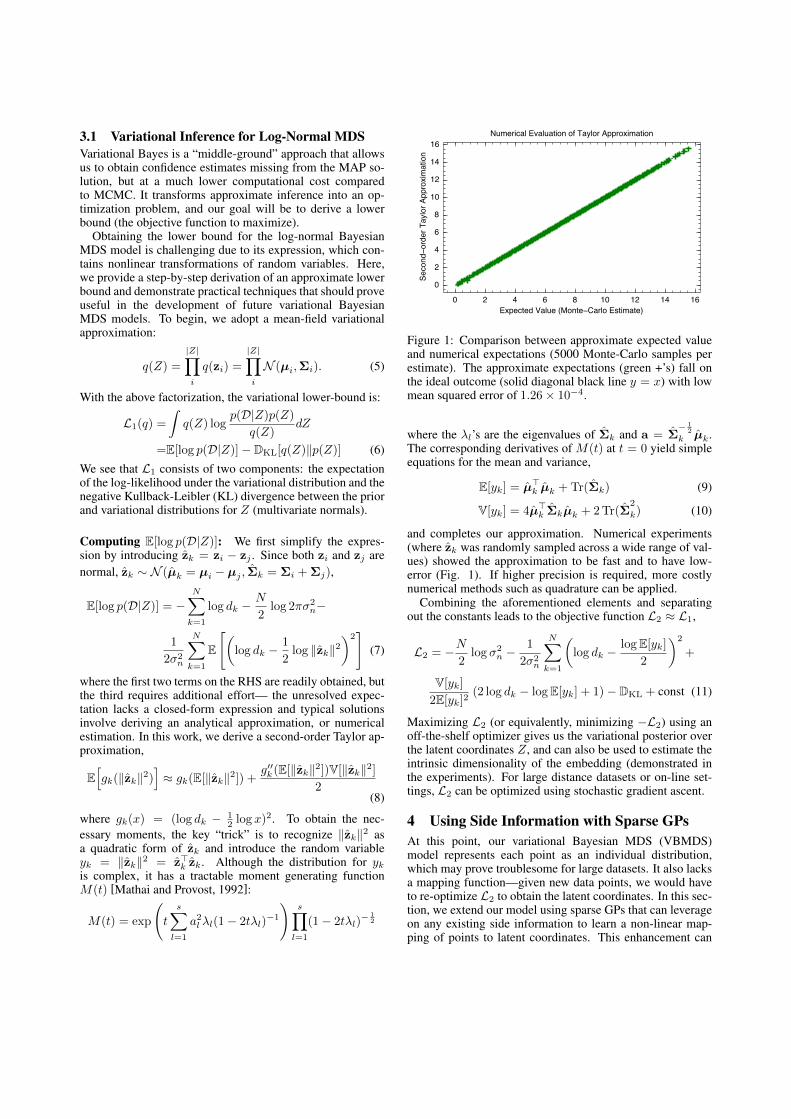
Figure 1: Comparison between approximate expected valueand numerical expectations (5000 Monte-Carlo samples perestimate). The approximate expectations (green +’s) fall onthe ideal outcome (solid diagonal black line y = x) with lowmean squared error of 1.26⇥ 10

�4.

where the �

l

’s are the eigenvalues of ˆ

⌃

k

and a =

ˆ

⌃

� 12

k

ˆµk

.The corresponding derivatives of M(t) at t = 0 yield simpleequations for the mean and variance,

E[yk

] =

ˆµ>k

ˆµk

+Tr(

ˆ

⌃

k

) (9)

V[yk

] = 4

ˆµ>k

ˆ

⌃

k

ˆµk

+ 2Tr(

ˆ

⌃

2

k

) (10)

and completes our approximation. Numerical experiments(where ˆ

z

k

was randomly sampled across a wide range of val-ues) showed the approximation to be fast and to have low-error (Fig. 1). If higher precision is required, more costlynumerical methods such as quadrature can be applied.

Combining the aforementioned elements and separatingout the constants leads to the objective function L2 ⇡ L1,

L2 = �N

2

log �

2n

� 1

2�

2n

NX

k=1

✓log d

k

� logE[yk

]

2

◆2

+

V[yk

]

2E[yk

]

2(2 log d

k

� logE[yk

] + 1)� DKL + const (11)

Maximizing L2 (or equivalently, minimizing �L2) using anoff-the-shelf optimizer gives us the variational posterior overthe latent coordinates Z, and can also be used to estimate theintrinsic dimensionality of the embedding (demonstrated inthe experiments). For large distance datasets or on-line set-tings, L2 can be optimized using stochastic gradient ascent.

4 Using Side Information with Sparse GPsAt this point, our variational Bayesian MDS (VBMDS)model represents each point as an individual distribution,which may prove troublesome for large datasets. It also lacksa mapping function—given new data points, we would haveto re-optimize L2 to obtain the latent coordinates. In this sec-tion, we extend our model using sparse GPs that can leverageon any existing side information to learn a non-linear map-ping of points to latent coordinates. This enhancement can

also lead to a more compact model, since some points arepresented indirectly.

Consider that Z is split into two mutually exclusive sets,Z = Z

p [ Z

x. Without loss of generality, assume that onlypoints in z

x

i

2 Z

x possess side information x

i

2 X 1. Em-ploying the variational inducing input scheme proposed by[Titsias, 2009] and [Hensman et al., 2013], we introduce aset of r inducing variables U = {u1, . . .ur

} (one for eachembedding dimension), and specify new priors,

p(z

x

il

|ul

) = N (k

>i

K

�1l

u

l

, k

ii

� k

>i

K

�1l

k

i

) (12)p(u

l

) = N (0,K

l

) (13)

where k

ij

= k(x

i

,x

j

), ki

= [k(x

i

,x

j

)]

m

j=1 and K

�1l

=

[k(x

i

,x

j

)]

m

i,j=1. The inducing inputs introduce conditionalindependencies between the latent function variables. As be-fore, we use a mean-field variational approximation,

q(Z

p

,Z

x

, U) = q(Z

p

)p(Z

x|U)q(U)

=

|Zp|Y

j

q(z

p

j

)

|Zx|Y

i

rY

l

p(z

x

il

|ul

)

rY

l

q(u

l

) (14)

where q(u

l

) = N (m

l

,S

l

) and q(z

j

) = N (µj

,⌃

j

). Theassociated variational lower-bound is

L3(q) =ZZZq(Z

p

, Z

x

, U) log

p(D|Zp

, Z

x

)p(U)

q(Z

p

)q(U)

dZ

p

dZ

x

dU

= E[log p(D|Zp

, Z

x

)]� DKL[q(U)kp(U)]�DKL[q(Z

p

)kp(Zp

)] (15)

where p(Z|U) inside the logarithm cancels out. The sparseGPs are assumed independent across the latent dimensions,which facilitates the derivation of the lower bound, and wehave new variational parameters parameters m

l

and S

l

as-sociated with the inducing variables (in addition to any GPkernel hyperparameters).

Again, the principal challenge is in computing the expec-tation of the likelihood, E[p(D|Zp

, Z

x

)]. Fortunately, we canre-use the derivations in the previous section, except that wenow compute the moments E[y

k

] and V[yk

] with respect toq(Z

p

)p(Z

x|U)q(U) instead of q(Z). Specifically, this ap-proach results in four possible cases, each requiring expecta-tions over different subsets of variables:

E[yk

] =

8>>><

>>>:

Ez

p

[y

k

] Case 1: fz

(z

p

i

, z

p

j

)

Ez

x

,u

[y

k

] Case 2: fz

(z

x

i

, z

x

j

)

Ez

x

,z

p

,u

[y

k

] Case 3: fz

(z

x

i

, z

p

j

)

Ez

x

,z

p

,u

[y

k

] Case 4: fz

(z

p

i

, z

x

j

)

(16)

and similarly for the variances. Case 1 arises when bothpoints are in Z

p and thus, the moments are those presentedin the previous section, i.e., eqns. (9) and (10).

1Extensions to more than two subsets (e.g., when points comefrom multiple domains) is straightforward, but we restrict our de-scription to a two-subset model for expositional simplicity.

Case 2: Here, both points have side information and arerepresented by the GPs. Starting from (9),

Ez

x

,u

[y

k

] = Eu

hˆµ>k

ˆµk

i+Tr(

ˆ

⌃

k

)

with ˆ

⌃

k

= Diag([�2kl

]

r

l=1)) and �

2kl

= k

ii

�k

>i

K

�1l

k

i

+k

jj

�k

>j

K

�1l

k

j

. It turns out that ˆµk

= [µ

kl

= (µ

il

� µ

jl

)]

r

l=1, isnormally distributed; recall that µ

il

= k

>i

K

�1l

u

l

and hence,

µ

kl

= k

>i

K

�1l

u

l

� k

>j

K

�1l

u

l

= b

>kl

u

l

(17)

where b>kl

= (k

i

�k

j

)

>K

�1l

. Since each u

l

is Gaussian, ˆµk

is also a Gaussian specified by,

ˆµk

= N⇣ˆ�k

=

⇥b

>kl

m

l

⇤r

l=1,

ˆ

⇤

k

= Diag⇣⇥

b

>kl

S

l

b

kl

⇤r

l=1

⌘⌘

As in the previous section, the moments of the quadratic formˆµ>k

ˆµk

are easily obtained via M(t),

Eu

hˆµ>k

ˆµk

i=

ˆ�>k

ˆ�k

+Tr(

ˆ

⇤

k

) (18)

Vu

hˆµ>k

ˆµk

i= 4

ˆ�>k

ˆ

⇤

k

ˆ�k

+ 2Tr(

ˆ

⇤

2

k

) (19)

The first moment is substituted into (17) to give,

Ez

x

,u

[y

k

] =

ˆ�>k

ˆ�k

+Tr(

ˆ

⇤

k

) + Tr(

ˆ

⌃

k

) (20)

Turning our attention to the variance and using same reason-ing as above (with some algebraic manipulation),

Vz

x

,u

[y

k

] = Eu

h4

ˆµ>k

ˆ

⌃

k

ˆµk

i+ 2Tr(

ˆ

⌃

2

k

) + Vu

hˆµ>k

ˆµk

i

= 4

ˆ�>k

(

ˆ

⌃

k

ˆ

⇤

k

ˆ

⌃

k

+

ˆ

⇤

k

)

ˆ�k

+ 2Tr((

ˆ

⌃

k

ˆ

⇤

k

)

2+

ˆ

⌃

2

k

+

ˆ

⇤

2

k

)

(21)

Cases 3 and 4: The third and fourth cases arise when thepoints come from each set Zx and Z

p, and can be treatedsimilarly. We build upon Case 2 by noting that

ˆ

z

k

⇠ N (

ˆµk

= [b

>kl

u

l

]

r

l=1 � µj

,

ˆ

⌃

k

= Diag[�2il

]

r

l=1 +⌃

j

)

where �2il

= k

ii

�k

>i

K

�1l

k

i

. This leads to a slightly differentGaussian distribution for ˆµ

k

= N (

ˆ�k

,

ˆ

⇤

k

) where

ˆ�k

=

⇥b

>kl

m

l

⇤r

l=1� µ

j

and ˆ

⇤

k

= Diaghb

>kl

S

l

b

kl

ir

l=1(22)

In the case that ˆzk

= z

p

i

� z

x

j

, the signs in the mean areflipped, ˆ�

k

= µj

�⇥b

>kl

m

l

⇤r

l=1. The above equations for ˆ�

k

and ˆ

⇤

k

(along with ˆ

⌃

k

) can be plugged into (20) and (21)derived in Case 2 to give the required central moments of y

k

.To complete L4 ⇡ L3, we replace the moments E[y

k

] andV[y

k

] in L2 (11), depending on the cases encountered (16).This extended model, the VBMDS-GP, completely general-izes the VBMDS since either set Zx and Z

p can be empty.Distinct from L2, there are no separate distributions for ele-ments of Zx. Instead, the latent coordinates are representedindirectly using the sparse GPs, which enables prediction oflatent coordinates using side information.

1 2 3 4 5−2000

−1500

−1000

−500

0

500

2D−lattice

Dimension

Lo

we

r−B

ou

nd

1 2 3 4 5−4

−3

−2

−1

0

1

2

3x 10

4 3D−lattice

Dimension

Lo

we

r−B

ou

nd

1 2 3 4 5−2.5

−2

−1.5

−1

−0.5

0

0.5x 10

4 Oilflow

Dimension

Lo

we

r−B

ou

nd

0 5 10

0.94

0.96

0.98

12D−lattice

Samples

Tru

stw

ort

hin

ess

0 5 10

0.94

0.96

0.98

1

Samples

Contin

uity

0 5 10

0.985

0.99

0.995

13D−lattice

Samples

Tru

stw

ort

hin

ess

0 5 10

0.985

0.99

0.995

1

Samples

Contin

uity

0 5 100.975

0.98

0.985

0.99

0.995

1Oilflow

Samples

Tru

stw

ort

hin

ess

0 5 10

0.98

0.985

0.99

0.995

1

Samples

Contin

uity

1 s.d.2 s.d.3 s.d.

0 5 10

0.94

0.96

0.98

12D−lattice

Samples

Tru

stw

ort

hin

ess

0 5 10

0.94

0.96

0.98

1

Samples

Co

ntin

uity

0 5 10

0.985

0.99

0.995

13D−lattice

Samples

Tru

stw

ort

hin

ess

0 5 10

0.985

0.99

0.995

1

Samples

Co

ntin

uity

0 5 100.975

0.98

0.985

0.99

0.995

1Oilflow

Samples

Tru

stw

ort

hin

ess

0 5 10

0.98

0.985

0.99

0.995

1

Samples

Co

ntin

uity

1 s.d.2 s.d.3 s.d.

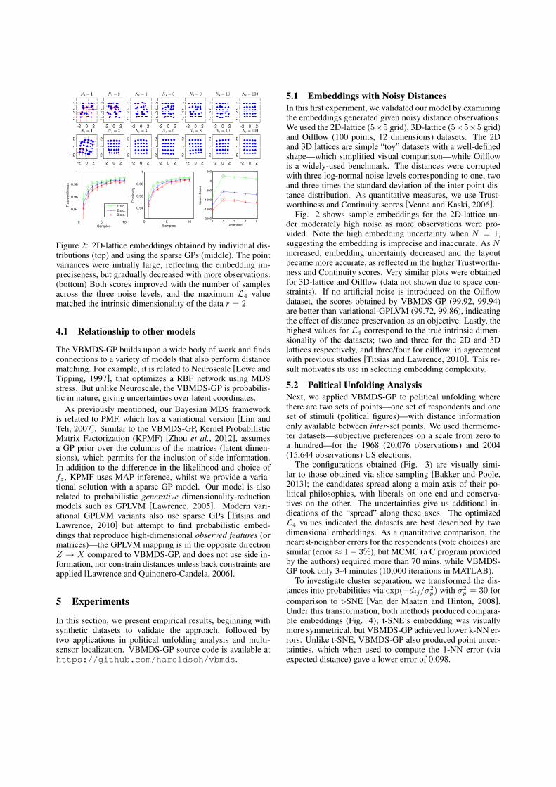
Figure 2: 2D-lattice embeddings obtained by individual dis-tributions (top) and using the sparse GPs (middle). The pointvariances were initially large, reflecting the embedding im-preciseness, but gradually decreased with more observations.(bottom) Both scores improved with the number of samplesacross the three noise levels, and the maximum L4 valuematched the intrinsic dimensionality of the data r = 2.

4.1 Relationship to other models

The VBMDS-GP builds upon a wide body of work and findsconnections to a variety of models that also perform distancematching. For example, it is related to Neuroscale [Lowe andTipping, 1997], that optimizes a RBF network using MDSstress. But unlike Neuroscale, the VBMDS-GP is probabilis-tic in nature, giving uncertainties over latent coordinates.

As previously mentioned, our Bayesian MDS frameworkis related to PMF, which has a variational version [Lim andTeh, 2007]. Similar to the VBMDS-GP, Kernel ProbabilisticMatrix Factorization (KPMF) [Zhou et al., 2012], assumesa GP prior over the columns of the matrices (latent dimen-sions), which permits for the inclusion of side information.In addition to the difference in the likelihood and choice off

z

, KPMF uses MAP inference, whilst we provide a varia-tional solution with a sparse GP model. Our model is alsorelated to probabilistic generative dimensionality-reductionmodels such as GPLVM [Lawrence, 2005]. Modern vari-ational GPLVM variants also use sparse GPs [Titsias andLawrence, 2010] but attempt to find probabilistic embed-dings that reproduce high-dimensional observed features (ormatrices)—the GPLVM mapping is in the opposite directionZ ! X compared to VBMDS-GP, and does not use side in-formation, nor constrain distances unless back constraints areapplied [Lawrence and Quinonero-Candela, 2006].

5 Experiments

In this section, we present empirical results, beginning withsynthetic datasets to validate the approach, followed bytwo applications in political unfolding analysis and multi-sensor localization. VBMDS-GP source code is available athttps://github.com/haroldsoh/vbmds.

5.1 Embeddings with Noisy DistancesIn this first experiment, we validated our model by examiningthe embeddings generated given noisy distance observations.We used the 2D-lattice (5⇥5 grid), 3D-lattice (5⇥5⇥5 grid)and Oilflow (100 points, 12 dimensions) datasets. The 2Dand 3D lattices are simple “toy” datasets with a well-definedshape—which simplified visual comparison—while Oilflowis a widely-used benchmark. The distances were corruptedwith three log-normal noise levels corresponding to one, twoand three times the standard deviation of the inter-point dis-tance distribution. As quantitative measures, we use Trust-worthiness and Continuity scores [Venna and Kaski, 2006].

Fig. 2 shows sample embeddings for the 2D-lattice un-der moderately high noise as more observations were pro-vided. Note the high embedding uncertainty when N = 1,suggesting the embedding is imprecise and inaccurate. As Nincreased, embedding uncertainty decreased and the layoutbecame more accurate, as reflected in the higher Trustworthi-ness and Continuity scores. Very similar plots were obtainedfor 3D-lattice and Oilflow (data not shown due to space con-straints). If no artificial noise is introduced on the Oilflowdataset, the scores obtained by VBMDS-GP (99.92, 99.94)are better than variational-GPLVM (99.72, 99.86), indicatingthe effect of distance preservation as an objective. Lastly, thehighest values for L4 correspond to the true intrinsic dimen-sionality of the datasets; two and three for the 2D and 3Dlattices respectively, and three/four for oilflow, in agreementwith previous studies [Titsias and Lawrence, 2010]. This re-sult motivates its use in selecting embedding complexity.

5.2 Political Unfolding AnalysisNext, we applied VBMDS-GP to political unfolding wherethere are two sets of points—one set of respondents and oneset of stimuli (political figures)—with distance informationonly available between inter-set points. We used thermome-ter datasets—subjective preferences on a scale from zero toa hundred—for the 1968 (20,076 observations) and 2004(15,644 observations) US elections.

The configurations obtained (Fig. 3) are visually simi-lar to those obtained via slice-sampling [Bakker and Poole,2013]; the candidates spread along a main axis of their po-litical philosophies, with liberals on one end and conserva-tives on the other. The uncertainties give us additional in-dications of the “spread” along these axes. The optimizedL4 values indicated the datasets are best described by twodimensional embeddings. As a quantitative comparison, thenearest-neighbor errors for the respondents (vote choices) aresimilar (error ⇡ 1� 3%), but MCMC (a C program providedby the authors) required more than 70 mins, while VBMDS-GP took only 3-4 minutes (10,000 iterations in MATLAB).

To investigate cluster separation, we transformed the dis-tances into probabilities via exp(�d

ij

/�

2p

) with �

2p

= 30 forcomparison to t-SNE [Van der Maaten and Hinton, 2008].Under this transformation, both methods produced compara-ble embeddings (Fig. 4); t-SNE’s embedding was visuallymore symmetrical, but VBMDS-GP achieved lower k-NN er-rors. Unlike t-SNE, VBMDS-GP also produced point uncer-tainties, which when used to compute the 1-NN error (viaexpected distance) gave a lower error of 0.098.

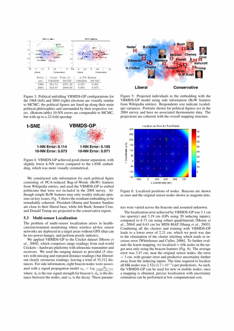
Data- Comp. Time (s) k-NN Errorset VBMDS MCMC VBMDS MCMC1968 254.74 4371.42 0.231 0.2612004 222.07 4888.60 0.085 0.075

Liberal Conservative Liberal Conservative

Figure 3: Political unfolding VBMDS-GP configurations forthe 1968 (left) and 2004 (right) elections are visually similarto MCMC; the political figures are lined up along their mainpolitical philosophies and surrounded by their respective vot-ers. (Bottom table) 10-NN errors are comparable to MCMC,but with up to a 22-fold speedup.

t-SNE VBMDS-GP

1-NN Error: 0.10510-NN Error: 0.071

1-NN Error: 0.11410-NN Error: 0.073

Figure 4: VBMDS-GP achieved good cluster separation, withslightly lower k-NN errors compared to the t-SNE embed-ding, which was more visually symmetrical.

We constructed side information for each political figureconsisting of PCA-reduced Bag-of-Words (BoW) featuresfrom Wikipedia entries, and used the VBMDS-GP to embedpoliticians that were not included in the 2004 survey. Al-though simple BoW features may only weakly indicate opin-ions on key issues, Fig. 5 shows the resultant embedding to beremarkably coherent: President Obama and Senator Sandersare close to their liberal base, while Jeb Bush, Senator Cruz,and Donald Trump are projected to the conservative region.

5.3 Multi-sensor LocalizationThe problem of multi-sensor localization arises in health-care/environment monitoring where wireless ad-hoc sensornetworks are deployed in a target areas without GPS (that canbe too power-hungry, and perform poorly indoors).

We applied VBMDS-GP to the Cricket dataset [Moore et

al., 2004], which comprises range readings from real-worldCrickets—hardware platforms with ultrasonic transmitter andreceivers. We used the ranging dataset as provided (5 clus-ters with missing and repeated distance readings) but filtered-out clearly erroneous readings, leaving a total of 35,312 dis-tances. For side information, eight beacon nodes were associ-ated with a signal propagation model s

bi

= log

A

b

(1000+d

bi

)↵b

where Ab

is the raw signal strength for beacon b, dbi

is the dis-tance between the nodes, and ↵

b

is the decay. These parame-

J. Bush

Trump

Cruz

Ashcroft

CheneyMcCainSanders

Obama

B.Clinton

H.Clinton

KerryEdwards

Nader

Liberal Conservative

Powell

Reagan

G.W.BushL.Bush

Figure 5: Projected individuals to the embedding with theVBMDS-GP model using side information (BoW featuresfrom Wikipedia entries). Respondents size indicate (scaled-up) variances. Portraits shown for political figures not in the2004 survey and have no associated thermometer data. Theprojections are coherent with the overall mapping structure.

Figure 6: Localized positions of nodes. Beacons are shownas stars and the original sensor nodes shown as magenta dots.

ters were varied across the beacons and assumed unknown.The localization error achieved by VBMDS-GP was 3.1 cm

(no sparsity) and 3.19 cm (GPs using 20 inducing inputs),compared to 6.73 cm using robust quadrilaterals [Moore et

al., 2004] and 6.63 cm for MDS-MAP [Shang et al., 2003].Combining all the clusters and training with VBMDS-GPleads to a lower error of 2.21 cm, which we posit was dueto the elimination of the cluster stitching which tends to in-crease error [Whitehouse and Culler, 2006]. To further eval-uate the learnt mapping, we localized ⇡ 68k nodes in the tar-get area only using the beacon features (Fig. 6). The averageerror was 3.47 cm; near the original sensor nodes, the error< 3 cm, with greater error and predictive uncertainty furtheraway from the inducing inputs. The time required to localizeall 68k nodes was 2.52s (3.7⇥10

�5s per prediction). As such,the VBMDS-GP can be used for new or mobile nodes; oncea mapping is obtained, precise localization with uncertaintyestimation can be performed at low computational cost.

6 Summary and ConclusionThis paper presented a computationally efficient variationalBayesian MDS model that leverages upon side informationand produces distance-preserving probabilistic embeddings.In the political unfolding task, VBMDS-GP produced em-beddings comparable to MCMC at a fraction of the compu-tational cost, and projected novel political candidates coher-ently to the embedding using only side information. Positiveresults were also observed for the localization task where theVBMDS-GP errors were half that of competing methods.

Given appropriate distance data, VBMDS-GP is applicableto a variety of tasks with side information, e.g., collaborativefiltering with product description and user profiles, social net-work visualization with node attributes, and document/imageclustering with meta-data. In general, we expect VBMDS-GPto perform well when the distance observations (plus discrep-ancy due to dimensionality difference) are approximately log-normal. As future work, alternative likelihoods can be usedwithin the Bayesian MDS framework to better suit other do-mains and to induce embeddings of different flavors.

AcknowledgmentsThank you to Scott Sanner for his helpful and constructivecomments.

References[Bakker and Poole, 2013] Ryan Bakker and Keith T Poole.

Bayesian metric multidimensional scaling. Political Anal-

ysis, 21(1):125–140, 2013.[Borg and Groenen, 2005] Ingwer Borg and Patrick JF Groe-

nen. Modern multidimensional scaling: Theory and appli-

cations. Springer, 2005.[Hashimoto et al., 2015] Tatsunori B. Hashimoto, David

Alvarez-Melis, and Tommi S. Jaakkola. Word, graph andmanifold embedding from Markov processes. In NIPS

2015 Workshop on Nonparametric Methods for Large

Scale Representation Learning, 2015.[Hensman et al., 2013] James Hensman, Nicolo Fusi, and

Neil D Lawrence. Gaussian Processes for Big Data. InUncertainty in Artificial Intelligence (UAI-13), 2013.

[Hinton and Roweis, 2002] Geoffrey E Hinton and Sam TRoweis. Stochastic neighbor embedding. In NIPS, pages833–840, 2002.

[Iyyer et al., 2014] Mohit Iyyer, Jordan L Boyd-Graber,Leonardo Max Batista Claudino, Richard Socher, and HalDaume III. A neural network for factoid question answer-ing over paragraphs. In EMNLP, pages 633–644, 2014.

[Lawrence and Quinonero-Candela, 2006] Neil D Lawrenceand Joaquin Quinonero-Candela. Local distance preserva-tion in the GP-LVM through back constraints. In Proc. of

the 23rd Intl. Conf on Machine learning, pages 513–520,2006.

[Lawrence, 2005] Neil Lawrence. Probabilistic non-linearprincipal component analysis with gaussian process latentvariable models. The Journal of Machine Learning Re-

search, 6:1783–1816, 2005.

[Lim and Teh, 2007] Yew Jin Lim and Yee Whye Teh. Vari-ational Bayesian Approach to Movie Rating Prediction.Proceedings of KDD Cup and Workshop, pages 15–21,2007.

[Lowe and Tipping, 1997] David Lowe and Michael E Tip-ping. Neuroscale: novel topographic feature extraction us-ing RBF networks. In Advances in Neural Information

Processing Systems (NIPS), pages 543–549, 1997.[Mathai and Provost, 1992] Arakaparampil M Mathai and

Serge B Provost. Quadratic forms in random variables:theory and applications. Journal of the American Statisti-

cal Association, 1992.[Mikolov et al., 2013] Tomas Mikolov, Quoc V Le, and Ilya

Sutskever. Exploiting similarities among languages formachine translation. arXiv preprint arXiv:1309.4168,2013.

[Moore et al., 2004] David Moore, John Leonard, DanielaRus, and Seth Teller. Robust distributed network local-ization with noisy range measurements. In Proc. of the

2nd Intl. Conf. on Embedded Networked Sensor Systems,pages 50–61. ACM, 2004.

[Pennington et al., 2014] Jeffrey Pennington, RichardSocher, and Christopher D Manning. GloVe: GlobalVectors for Word Representation. Proceedings of the 2014

Conference on Empirical Methods in Natural Language

Processing, pages 1532–1543, 2014.[Salakhutdinov and Mnih, 2008] R Salakhutdinov and

A Mnih. Probabilistic Matrix Factorization. NIPS, pages1257–1264, 2008.

[Sammon, 1969] John W Sammon. A nonlinear mappingfor data structure analysis. IEEE Trans. on Computers,18(5):401–409, 1969.

[Shang et al., 2003] Yi Shang, Wheeler Ruml, Ying Zhang,and Markus PJ Fromherz. Localization from mere con-nectivity. In Proc. of the 4th ACM Int. Symp. on Mobile

ad hoc networking & computing, pages 201–212. ACM,2003.

[Shepard, 1980] Roger N Shepard. Multidimensional scal-ing, tree-fitting, and clustering. Science, 210(4468):390–398, 1980.

[Tenenbaum et al., 2000] Joshua B Tenenbaum, VinDe Silva, and John C Langford. A global geomet-ric framework for nonlinear dimensionality reduction.Science, 290(5500):2319–2323, 2000.

[Titsias and Lawrence, 2010] Michalis K Titsias and Neil DLawrence. Bayesian Gaussian Process Latent VariableModel. In AISTATS, pages 844–851, 2010.

[Titsias, 2009] Michalis Titsias. Variational Learning of In-ducing Variables in Sparse Gaussian Processes. In AIS-

TATS, pages 567–579, 2009.[Torgerson, 1952] Warren S Torgerson. Multidimensional

scaling: I. Theory and method. Psychometrika, 17(4):401–419, 1952.

[Van der Maaten and Hinton, 2008] Laurens Van der Maatenand Geoffrey Hinton. Visualizing data using t-SNE.JMLR, 9(2579-2605):85, 2008.

[Venna and Kaski, 2006] Jarkko Venna and Samuel Kaski.Local multidimensional scaling. Neural Networks,19(6):889–899, 2006.

[Vilnis and McCallum, 2015] Luke Vilnis and Andrew Mc-Callum. Word Representations via Gaussian Embedding.In ICLR, 2015.

[Whitehouse and Culler, 2006] Kamin Whitehouse andDavid Culler. A robustness analysis of multi-hop ranging-based localization approximations. In Proc. of the 5th

Intl. Conf. on Information Processing in Sensor Networks,pages 317–325. ACM, 2006.

[Zhou et al., 2012] Tinghui Zhou, H Shan, A Banerjee, andGuillermo Sapiro. Kernelized Probabilistic Matrix Factor-ization: Exploiting Graphs and Side Information. In SIAM

International Conference on Data Mining (SDM), pages914–925, 2012.