• \ I ;

• ,I'

! I

Distribution Of Dredged Material At The Rockland Disposal Site May 1985

Disposal Area Monitoring System DAMOS

Contribution 50 March 1988

US Army Corps of Engineers New England Division

DISTRIBUTION OF DREDGED MATERIAL AT THE ROCKLAND DISPOSAL SITE

MAY 1985

CONTRIBUTION #50

17 JANUARY 1988

Report No. SAlC - 85n533&C50

Contract No. DACW-85-D-0008 Work Order No.2

Submitted to:

Regulatory Branch New England Division

U.S. Army Corps of Engineers 424 Trapelo Road

Waltham, MA 02254-9149

Submitted by:

Science Applications International Corporation Admiral's Gate

221 Third Street Newport, Rl 02840

(401) 847-4210

US Army Corps of Engineers New England Division

1.0

2.0

3.0

4.0

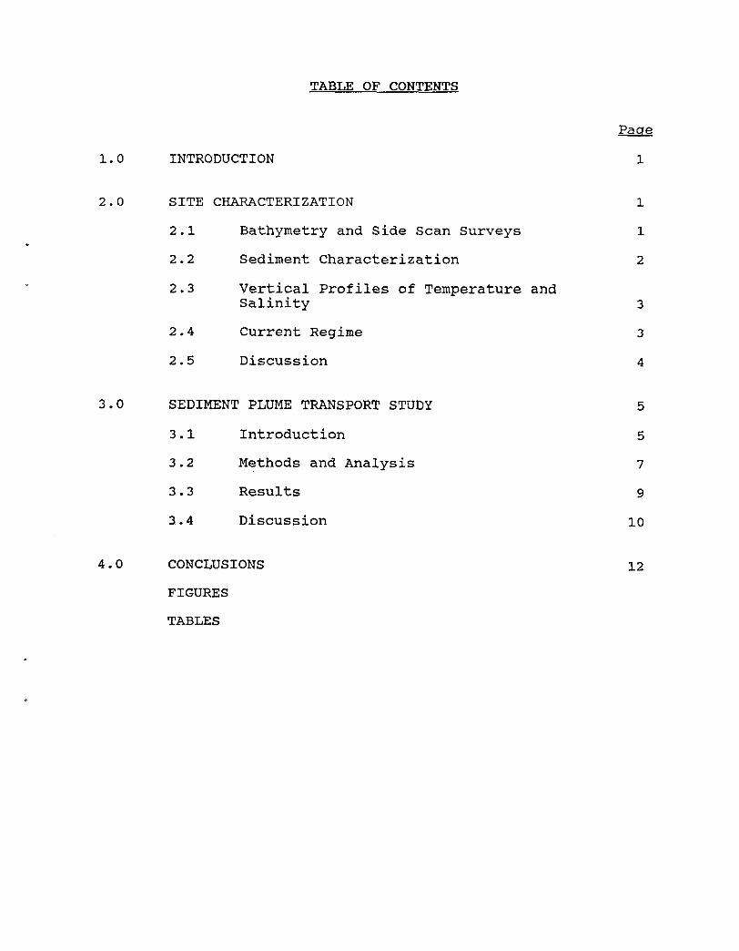
TABLE OF CONTENTS

INTRODUCTION

SITE CHARACTERIZATION

2.1

2.2

2.3

2.4

2.5

Bathymetry and Side Scan Surveys

Sediment Characterization

Vertical Profiles of Temperature and Salinity

Current Regime

Discussion

SEDIMENT PLUME TRANSPORT STUDY

3.1 Introduction

3.2 Methods and Analysis

3.3 Results

3.4 Discussion

CONCLUSIONS

FIGURES

TABLES

1

1

1

2

3

3

4

5

5

7

9

10

12

Figure 1-1

Figure 2-1

Figure 2-2

Figure 2-3

Figure 2-4

Figure 2-5

Figure 2-6

Figure 2-7

Figure ~-8

Figure 2-9

Figure 2-10a

Figure 2-10b

Figure 2-11a

Figure 2-11b

Figure 2-12

LIST OF FIGURES

Rockland Disposal Area.

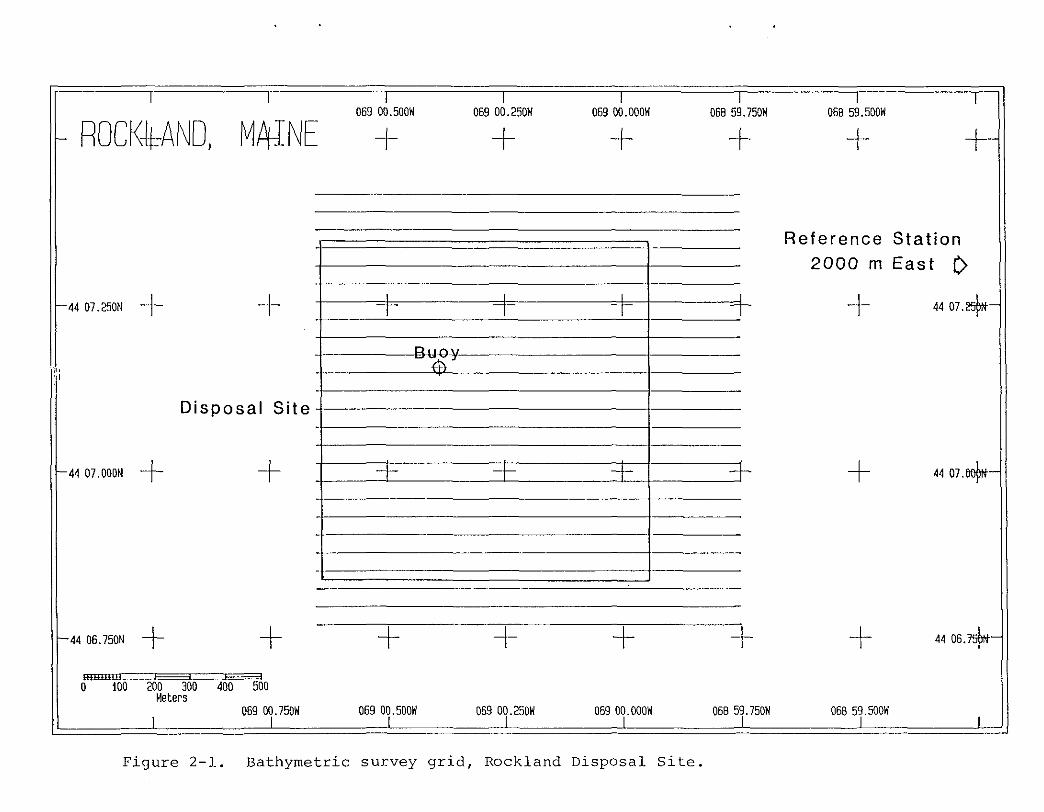
Bathymetric survey grid, Rockland Disposal site.

Bathymetric contour plot of Rockland Disposal Site, 20 May 1985.

Results of the side scan survey conducted at Rockland, ME on 20 May 1985.

Side scan record showing high reflectance at center of disposal area.

Side scan record showing circular area of reflectance indicating a single dump.

Side scan record showing result of disposal occurring underway in a turn.

Sediment sampling locations during the May 1985 survey.

Sediment station sampling locations during the September 1984 survey.

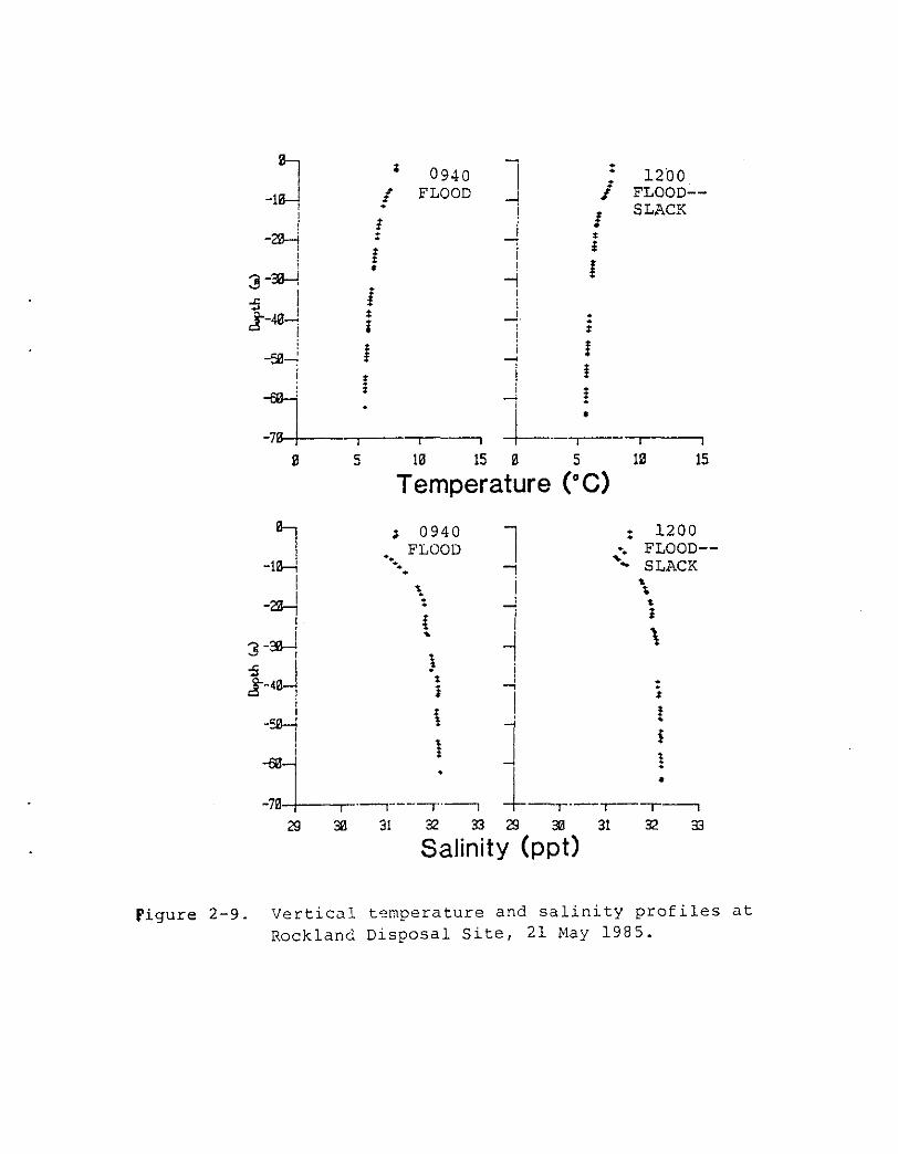
vertical temperature and salinity pro­files at Rockland Disposal Site, 21 May 1985.

vertical temperature profiles at Rockland Disposal Site, 22 May 1985.

Salinity profiles at Rockland Disposal site, 22 May 1985.

vertical temperature profiles at Rockland Disposal Site, 23 May 1985.

vertical salinity profiles at Rockland Disposal Site, 23 May 1985.

vertical temperature and salinity pro­files at Rockland Disposal Site, 24 May 1985.

Figure 2-13

Figure 2-14

Figure 3-1

Figure 3-2

Figure 3-3

Figure 3-4

Figure 3-5

Figure 3-6

Figure 3-7

LIST OF FIGURES (cant.)

Three-hour low pass (3-HLP) time series of temperature, current speed, and direction at Rockland Disposal Site at a depth of 10m, 21 May to 11 June 1985.

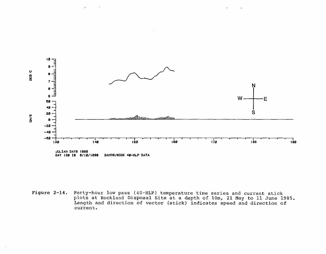
Forty-hour low pass (40-HLP) temperature time series and current stick plots at Rockland Disposal site at a depth of 10m, 21 May to 11 June 1985.

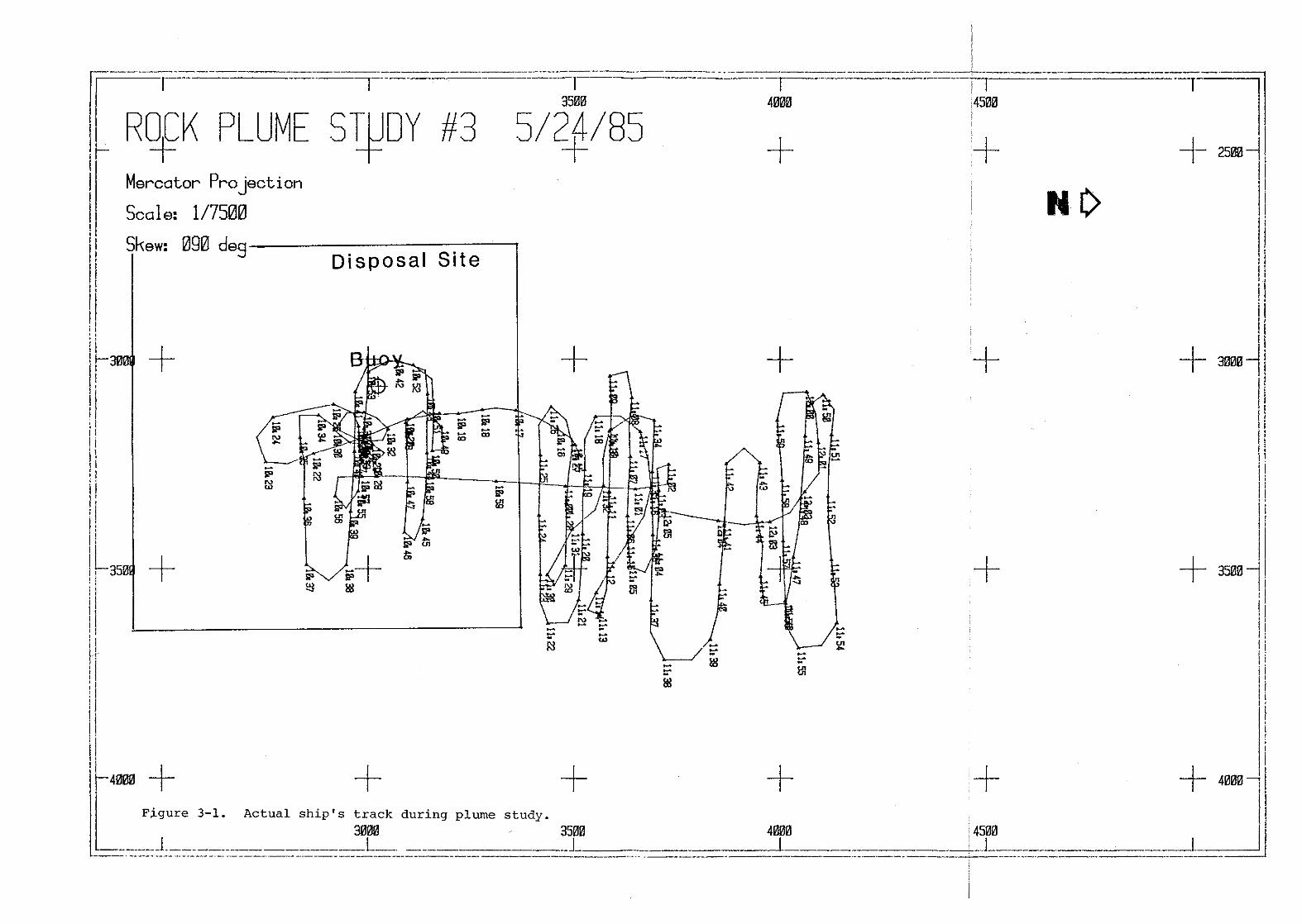
Actual ship's track during plume study.

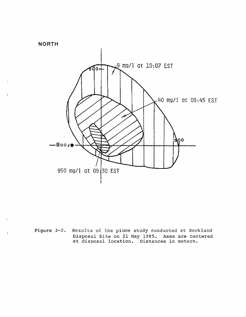
Results of the plume study conducted at Rockland Disposal site on 21 May 1985.

Photographs of the acoustic record for the plume study of 21 Mc:.y 1985.

Results of plume study conducted at Rockland Disposal Site on 22 May 1985.

Photographs of the acoustic record for the plume study of 22 May 1985.

Results of the plume study conducted at Rockland Disposal Site on 24 May 1985.

Photographs of the acoustic record for the plume study of 24 May 1985.

Table 2-1

Table 2-2

Table 2-3

Table 3-1

LIST OF TABLES

Qualitative Sediment Characterization at Rockland Disposal site, May 1985

Results of Sediment Chemical Analysis at Rockland Disposal site, october 1984

Results of the Bivariate Analysis of 3-HLP Current Meter Data Collected at Rockland at a Depth of 10m, 21 May to 11 June 1935

Estimates of Material in Water Column After Disposal

1.0 INTRODUCTION

The Rockland Disposal site is located in the center of West Penobscot Bay (Fig. 1-1), 3.3 NM northeast of the Rockland Breakwater. This site was first used during October 1973-February 1974 for disposal of approximately 69,000 m3 (90,200 yds3 ) of material from Rockland Harbor. The disposal site is a 0.5 nautical mile square centered at 44°07.01'N, 69°00.3'W. Water depths within the disposal area range from 65 to 80 meters. The disposal site is marked with a buoy deployed and maintained by the us coast Guard.

An earlier baseline survey of the disposal site was conducted during the period 24 september - 2 October 1984 to determine existing conditions of the bottom before the start of dredging projects from the Searsport area. This survey included precision bathymetry, sediment characterization (chemical and physical), a side scan survey, and REMOTS® sediment profiling.

The present study was conducted during the period 19-24 May 1985 to assess the transport of dredged material during disposal operations and to perform bathymetric and side scan surveys of the area after approximately 360,000 yd3 (275,400 m3 ) of dredged material from the Searsport project had been deposited. vertical profiles of temperature and salinity were conducted, and current meters were deployed for approximately one month at the disposal site. The results of the data analysis were used to estimate the percent of material expected to reach the bottom during disposal operations and to delineate the extent of dredged material throughout the disposal site.

2.0 SITE CHARACTERIZATION

2.1 Bathymetry and Side Scan Surveys

A bathymetric survey was performed over an area 1200 m by 1200 m' surrounding the disposal site. The survey, comprised of 50 lanes, 1200 m long, spaced 25 meters apart, was accomplished using a 24 kHz fathometer system operating in conjunction with the SAlC Navigation and Data Acquisition System which is based on an HP 9920 microcomputer system.

Figure 2-1 shows the relation to the disposal site, disposal buoy and the location of for the sediment sampling program.

bathymetric the present the Reference

survey area in location of the Site established

A contour chart of depths at the disposal site is shown in Figure 2-2a. The site is characterized by a depression which is well-defined in the northern portion of the site, but widens and shoals toward the south, completely losing its identity over

1

-------------------------------------- ------- ---

the southern half of the site. Depths range from about 65 meters to 80 meters within the surveyed area. Comparison with the bathymetric survey conducted in September 1984 (Figure 2-2b) reveals no significant development of a disposal mound near the buoy location.

Figure 2-3 shows the results of the side scan survey at the Rockland site conducted in May 1985. The outlined area indicates the presence of intermediate acoustic reflectance that could be caused by soft natural bottom or old dredged material. The small dark areas show the location of higher acoustic reflectance characteristic of dredged material. The central area of the site is well covered by dredged material and is surrounded by individual disposal events. Long narrow areas probably indicate disposal that occurred underway or during a turn.

Figure 2-4 is a photograph of the side scan record at the center of the area showing this high acoustic reflectance. Figure 2-5 shows a circular area, probably the result of a single dump. Figure 2-6 shows the result of disposal occurring during a turn. The side scan records did not detect any large accumulation in the form of a mound.

2.2 Sediment Characterization

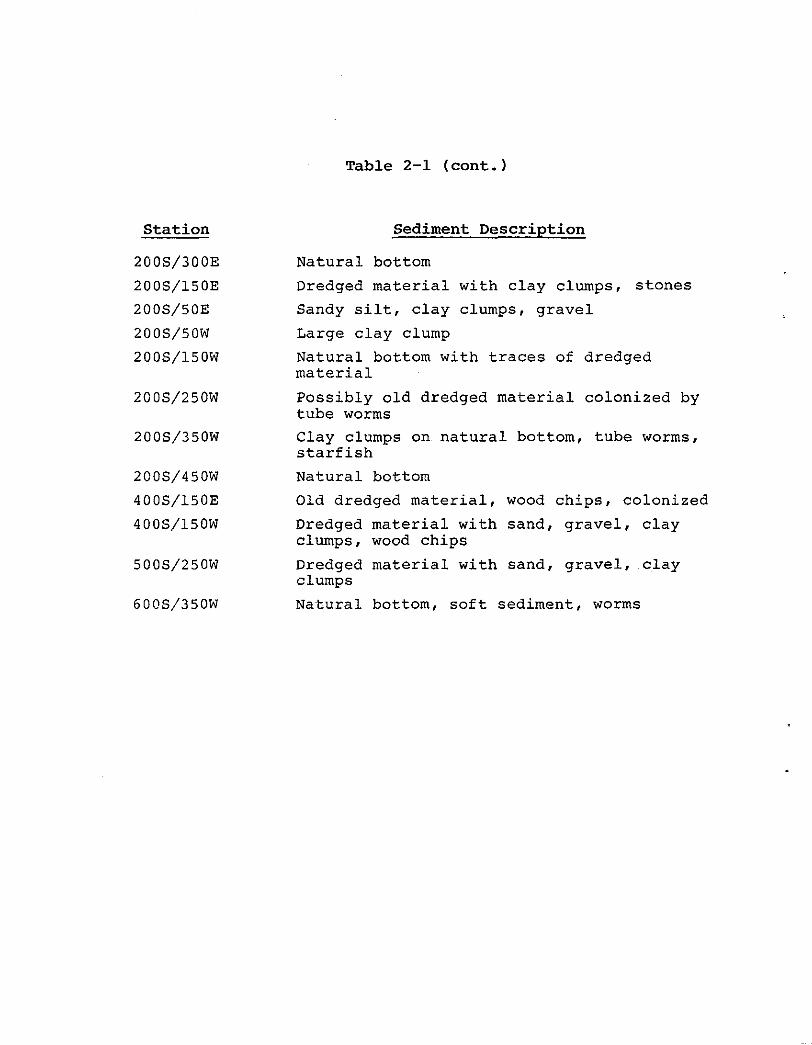
Figure 2-7 shows the location of sediment samples taken at the Rockland Disposal site to visually characterize the bottom and detect the extent of dredged material. Table 2-1 describes the sediment collected at each station with a 0.1 m2 Smi th­MacIntyre grab sampler. The pattern of stations sampled was determined by visually identifying dredged material in the grab and proceeding until natural bottom was encountered. The spatial delineation of dredged material from the grab samples compared well with the areas of high reflectance measured with side scan sonar. Minor discrepancies resulted from the patchy nature of single dump loads. The areas of intermediate reflectance could indicate the presence of old dredged material.

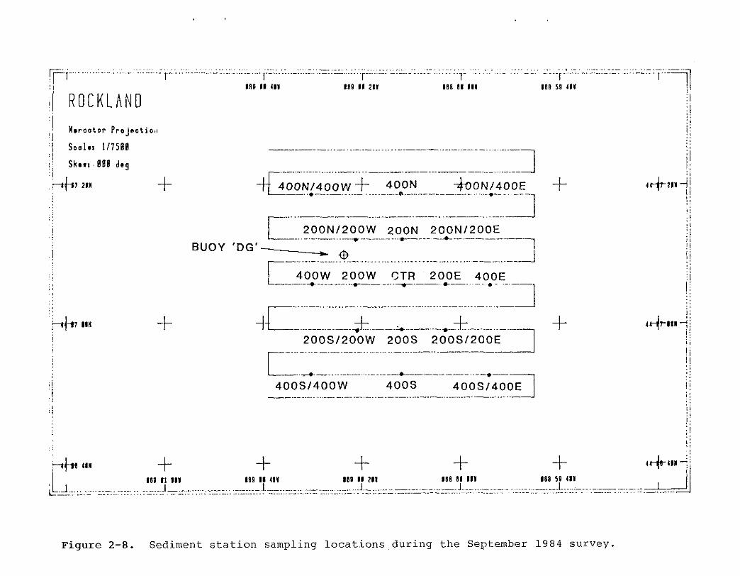
During the September 1984 survey, sediment samples were collected at stations on North-South, East-west, Northwest­Southeast, and Northeast-Southwest transects (Fig. 2-8), as well as at the Reference Site (2000m east). Table 2-2 contains the results of the chemical analyses of the sediment samples.

The results of the chemical and physical analyses indicate little variation throughout the site. The physical tests indicate the similarity between locations with a pattern cornmon to most of the samples; olive in color, high percentage of fines (average about 90% and predominantly clays), low fine sand percentages (around 10%) and very little medium and coarse material (usually less than 1%). These values also occur at the

2

reference site. The only exception of note was at 200S where the amount of fine sand was 18%.

The chemical data also reflected this uniformity along the transects by showing rather small differences between individual location replicates. The concentrations for the trace metals were low throughout the area. COD and organics were typical for natural bottom silt/clay. An exception was at 200SW, where relatively high concentrations of oil and grease were found, most likely from the presence of dredged material. The results of the chemical analyses at a majority of the stations in the disposal area are similar with those from natural bottom. C:N ratios were mostly between 7 and 9 (typical of offshore natural sediment). Mg:Ca ratios averaged between 4-6, indicating relatively few shells. Dredged material may have influence at 400W; the Mg:ca ratios here averaged about 1 (relatively high in shells) and the C:N ratio averaged about 11 (typical of inshore harbors and estuaries). The variation in Mg:Ca and Fe results at 400NE may be caused by local natural bottom conditions and not dredged material.

2.3 vertical Profiles of Temperature and Salinity

On each day of the period 21 May 24 May 1985, vertical profiles for temperature and salinity were measured at the disposal buoy to determine the structure of the water column. Figures 2-9 to 2-12 show the temperature and salinity data collected each day. The temperature ranged from approximately 6·C at the bottom to II·C at the surface with a thermocl '.ne present at about 10 meters by 23 May. Salinity ranged from approximately 29.6 ppt at the surface to 32.2 ppt at the bottom. Throughout the tidal cycle, little effect was seen on the shape of the vertical profiles. Wind-driven water movement could account for changes in salinity and temperature at the surface. Certain vertical profiles are seen to contain fewer data points than others. This was due to intermittent data signals being received by the computer. Alternatively, data were recorded manually at specified depths.

2.4 CUrrent Regime

During the period 21 May to 11 June 1985, current measurements were made at Rockland in order to determine the overall current regime of the area. A string of two General oceanics current meters at depths of 10 meters and 60 meters was deployed about 300m SE of the disposal buoy. Due to a tape malfunction, no data were collected by the 60 meter instrument. Figure 2-13 presents the current speed and direction and temperature data for the observation period. These data have been 3-hour low pass filtered (3-HLP) to emphasize the tidal components.

3

The temperature trace reveals initial readings of approximately 6.4'C warming to an average value of 8.3'C with a maximum value of about 9.8'C. Higher temperatures are detected on the ebb tide as warmer waters from the shallower coastal areas flow by the disposal area.

The current direction varies in the N-S axis over the tidal cycle. The peak current velocities occur on the flood tide in the northerly direction with maximum values of approximately 40 cm/sec (Table 2-3). Table 2-3 presents the results of bivariate analysis of the current data (3-HLP) revealing the average current speed to be approximately 13 cm/sec. The current direction is northerly for approximately 50% (sum of 29.9 and 18.6%, see boxes in Table 2-3) of the period and southerly only 22% (sum of 16.7 and 5.2%) of the period. For 65% (sum of 27.1, 23.8 and 13.8%) of the period, the current velocities were in the range of 4-16 cm/sec. Only 13% (sum of 5.0, 3.6, 2.5, 1.3 and 0.4%) of the period saw velocities greater than 24 cm/sec (0.5 knots) .

Figure 2-14 presents the temperature data and a current stick plot for 40-hour low-pass filtered data (40-HLP). The temperature time series depicts the average values after the tidal component is removed. The net, non-tidal flow in the disposal area is consistently to the north-northeast quadrant at a maximum of approximately 15 cm/sec.

2.5 Discussion

The results of the bathymetric survey did not reveal the development of a disposal mound near the location of the disposal buoy. Rough estimates from scow logs of the volume of dredged material deposited between the September 1984 survey and the present one are approximately 360,000 yd3 (275,400 m3). This large volume of material would be expected to create a mound if controlled point disposal was conducted. A combination of factors including the depth at the disposal point (70 m), the wide scope (3 times the water depth) of buoys normally established by the US Coast Guard, and, apparently, a practice of depositing dredged material while the scow is underway has caused the material to be spread over a large area. Disposal of dredged material in a water depth of 70 m allows a significant amount of water to be entrained during the convective descent phase of disposal. A large percentage of the dredged material will then have a lower density due to the increased water content causing a slower descent and increased spreading from the initial disposal location.

Figure 2-3 shows the wide distribution of dredged material detected by the side scan sonar. The outline in the figure indicates the area of intermediate reflectance that usually signifies thin layers of dredged material. The pattern

4

of distribution suggests that some scows began material before and/or after reaching the However, a large percentage of the material accumulated southeast of the buoy.

deposi ting the disposal buoy. has apparently

A rough estimate of the amount and thickness of dredged material can be calculated using the approximate area of seafloor indicated by the side scan sonar survey to be covered with dredged material. Examination of Figure 2-3 shows an area roughly 700 by 700m square of intermediate acoustic reflectance, usually indicating dredged material. Assuming that approximately 275,400 m3 of material (estimated from scow logs) was evenly spread over this area, a layer of dredged material of approximately 0.5 m thickness could be expected. When considering that both the loss of interstitial water during descent and compaction after impact with the bottom would reduce the actual volume of material expected to be seen on the bottom by as much as 40% (Tavalaro, 1983), the thickness of the dredged material may actually be approximately 0.3 m. It would be difficult to confirm the presence of this layer with bathymetry in a depth of 70 m due to the limitations of available fathometer systems and a combination of errors associated with the speed of sound, tide, and navigation. More detailed study of this area with precision bathymetric surveys at a smaller lane spacing (25 m) would detect any significant topographic features caused by dredged material disposal while REMOTS® sediment profiling would be needed to accurately measure the thickness of the dredged material layer and determine its areal limits.

3.0 SEDIMENT PLUME TRANSPORT STUDY

3.1 Introduction

In order to assess the potential impact of dredged material disposal on the surrounding environment, a plume study was conducted to track suspended material in the water column after a disposal event. Three studies were performed during the period of 21 May to 24 May 1985. Although attempts were made to track plumes on both the flood and ebb tides, coordination of scow arrival and dumping, weather, and tide prevented studies occurring during ebb tide. However, because the dominant current feature is the flood tide (with maximum peak velocities and long durations), emphasis on the flood tide was warranted due to its greater potential for transport.

Multi-frequency acoustic profiling has been under investigation since 1975 as a means of measuring concentrations of suspended matter in the water column. Much of the work has been carried out by the NOAA Atlantic Oceanographic and Meteorological Laboratory in Miami. The work has included study of diffusion properties and acoustic measurements, as well as development of a model to describe the relationship between

5

concentrations of total suspended matter in the water column and acoustic profile observations. A diffusion model allowing prediction of diffusion velocities and spatial variation has been postulated and tested.

The following relevant observations are taken from a technical paper "SOME OBSERVATIONS ON DREDGED MATERIAL DUMPING IN THE NEW YOm: BIGHT", by Dr. John Proni and Dr. John Tsai at the NOAA-AOML facility.

1. spatial and temporal variation during diffusion following a dump predicts a two­process diffusion with different diffusion velocities and spatial variation. During the active phase, heavy materials settle through gravitation, reaching the bottom. The downward momentum may generate vertical mixing of the water column inside the plume, and resuspension from the bottom. During the passive diffusion phase, the sharp edges of the plume disappear and dissipate into the surrounding water. Rate of diffusion slows down as the particle size distribution changes from coarse heavy material to smaller, lighter particulate matter. This dual diffusion process was clearly observed during the dredged material dump in Massachusetts Bay in February 1983.

2. Acoustic backscatter measurements can be correlated with measurements of total suspended matter in the water column as:

I = a N

where I is acoustic intensity, N is the number of particles per unit volume, and a is assumed to depend on particle shape, size, density, compressibility and frequency. Direct and linear relationships are found between observed acoustic intensity and measured total suspended matter.

In the Rockland Disposal Area study, the following tasks were attempted:

1. Track and observe the extent dissipation and movement over a time following the dump.

6

of plume period of

2.

3.

3.2

Measure ambient and in-plume concentrations of total suspended matter by analyzing water samples taken in selected locations where acoustic intensity could also be observed.

Using the measured values of total suspended matter as "ground truth", make estimates of total suspended matter concentration based on acoustic backscatter measurement alone.

Methods and Analysis

The Datasonics Model DFS-2100 Acoustic Remote Sensing System was used at 200 kHz for performing the acoustic plume tracking. High power· output, low receiver noise levels and calibrated control of signal level allows monitoring of extremely low concentrations of material in the water column and acquisition of suspended sediment concentration levels when correlated with ground truth sampling.

In attempting to relate acoustic backscatter measurements in a plume of suspended particulate matter to quantitative concentration levels, one must measure the reflection, or backscattering characteristics of the material in the scattering volume of interest.

The echo or reverberation level received back at the towed vehicle transducer from particulate scatterers in the dredged material plume may be expressed as part of a standard sonar equation as follows: (See definition of terms below).

RL = SL - 40 Log R - 2aR + Sv + 10 Log V ( 1)

Equation 1 summarizes signal losses wi thin the water column. The acoustic receiver voltage output measured and recorded during a survey can be defined as follows:

out rIDS = RL + RS + GAIN

or

RL = out rms - RS - GAIN (2)

Equating equations 1 and 2 .

out rms = SL-(40 Log R + 2aR) + (Sv + 10 Log V) + RS + GAIN (3)

Definition of Terms

RL: Reverberation Level, from a random, homogeneous a defined volume of water.

or backscattered acoustic intensity distribution of scatterers throughout

7

---- ... _-----------------

SL: Source Level, a measure of on-axis acoustic intensity of the transmitted signal.

40 Log R + 2QR: Two way transmission loss from the transducer down to the scattering volume of interest and back to the transducer. The 40 Log R component is due to spherical spreading loss, while the 2QR loss is due to absorption (primarily a function of frequency).

~v + 10 Log V: A measure of the backscattering strength due to volume reverberation. It is the Sv term which will correlate with concentration of scatterers, or total suspended matter. V is a measure of the backscattering volume which will increase with depth as the volume of water encompassed by the acoustic signal increases due to the transducer beam pattern.

RS: Receive Sensitivity or transfer function of the receiving transducer in conversion of the echo pressure wave to an electrical voltage.

GAIN: Overall receiver gain, including Time varying Gain (TVG).

Examination of Model DFS-2100 Acoustic following:

Equation 3, when using the Datasonics Remote Sensing system, reveals the

1. The receiver gain incorporates TVG which compensates precisely for the 40 Log R + 2QR transmission loss term. These two terms then fallout of the equation. If overall gain is changed, however, the change must be factored into the calculations.

2. Receive sensitivity is a constant, determined by laboratory measurement. This term can be ignored in making concentration calculations from acoustic observations because relative concentration measurements, with respect to measured total suspended matter samples, are being made.

3. Source Level may remains constant. whenever a change

be ignored so long as it It must be accounted for

is made.

4. Vo rms' the measured receiver output, is then proportional to Sv + 10 Log V. V is a function of pulse width, equivalent beamwidth and range (R) from the transducer to scattering volume. V is a measure of the reverberating volume at any given depth.

8

For any given particle size distribution, the concentration of total suspended matter will be proportional to the measured rms voltage output of the receiver, when corrected for depth.

3.3 Results

The plume studies were conducted at disposal events when the towed scow was unloaded by opening the bottom doors. As soon as disposal was complete and the scow was underway, the research vessel, with navigational control and the Acoustic Remote Sensing System aboard, began executing patterns of parallel tracks to determine the boundaries of the plume. After the motion of the plume was determined, the ship's track was modified to continually encompass the boundaries. Figure 3-1 presents an actual ship's track followed during the first two hours of the plume study on 24 May 1985.

During each study, water samples were collected with Niskin water samplers as the acoustic sensing transducer passed through the plume. Sampling depths were determined from the acoustic results of a pass through the area immediately prior to sampling. The samples were analyzed for total suspended sediment (mg/l) and used to calibrate the output voltages from the acoustic record.

21 May 1985 Plume Study

The plume study began at 0920 EST as the scow began the disposal operation. One scow of 1575 cu yds (1205 m3 ) was dumped approximately 200 m east of the disposal buoy. The study was continued until 1051 EST. Low tide occurred at 0547 EST and high tide at 1157 EST. Flood tide was in progress during the survey, providing a N-NE flow. Figure 3-2 presents the results of the plume survey.

The area of heavy concentrations (averaging about 1000 mg/l, Fig. 3-3) occurred below a depth of 50m and did not extend far beyond the area directly beneath the disposal location. Within 15 minutes of the completion of the disposal operation, concentrations averaging approximately 40 mg/l (Fig. 3-3) occurred from a depth of 20 m to the bottom and extended approximately 300 m from the initial location in the N-NE quadrant. Within forty minutes of disposal, suspended sediment concentrations were averaging less than 10 mg/l (Fig. 3-3) at depths below 35 m and extended less than 500 m from the disposal point, still within the boundaries of the designated disposal site. Further surveying detected no significant levels of suspended sediment above background concentrations of 3-5 mg/l.

9

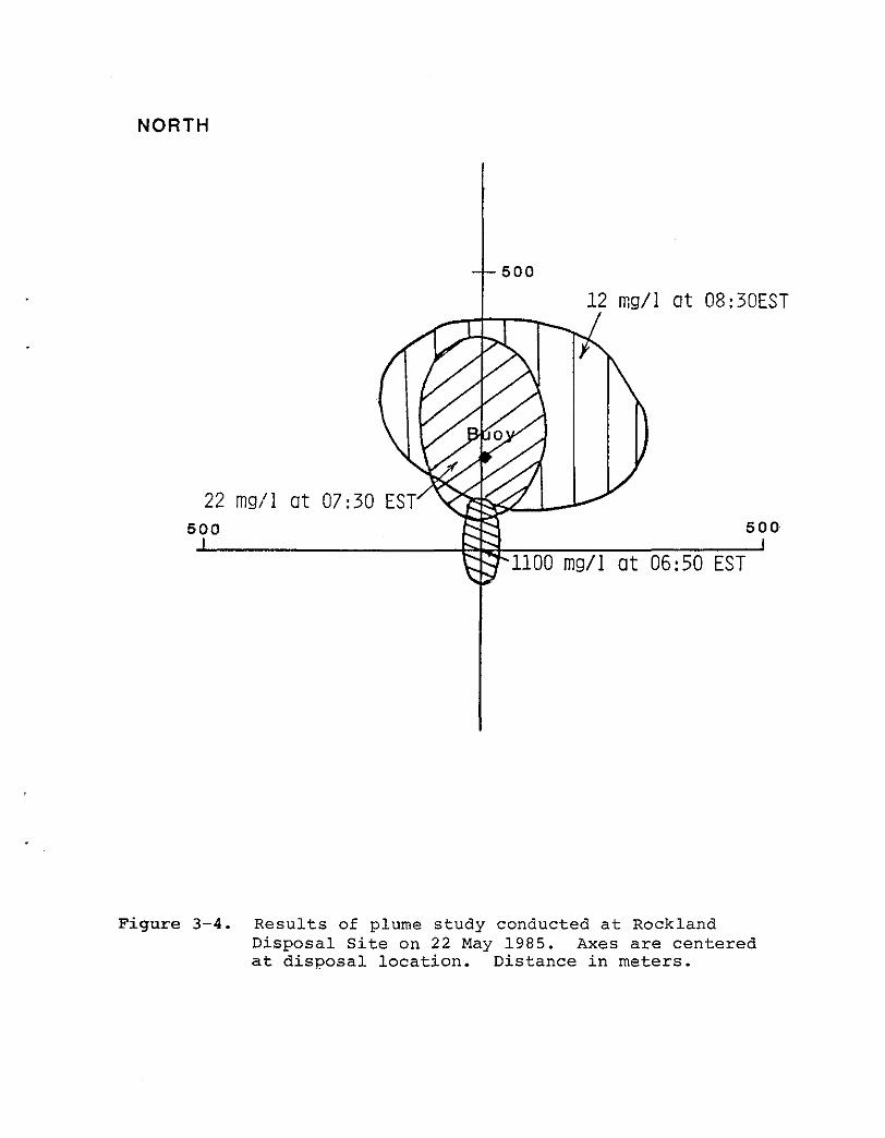
22 May 1985 Plume study

The second plume study began at 0645 as one scow of 1900 cu yds (1450 m3 ) completed disposal operations approximately 150 meters south of the disposal buoy (Fig. 3-4). with low tide occurring at 0623 EST, flood tide was just beginning to develop. Again, the heavy concentrations of suspended material, averaging greater than 1000 mg/l (Fig. 3-5), occurred directly beneath the disposal location throughout the water column. within forty minutes of disposal, concentrations averaging greater than 25 mg/l (Fig. 3-5) occurred below 30 m to the bottom and extended approximately 350 meters to the north. One hundred minutes after disposal, concentrations averaging only 12 mg/l (Fig. 3-5) occurred at depths below 50 m and extended less than 500 meters north-northeast of the disposal point, still within the disposal site.

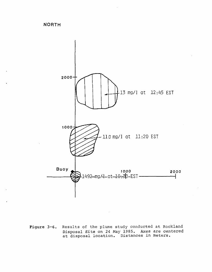
24 May 1985 Plume Study

The third plume study began at 1025 EST as two scows (tandem load) containing a total of 3640 cu yds (2780 m3 ) completed disposal operations within 50m SE of the disposal buoy (Fig. 3-6). with low tide occurring at 0744 EST and high tide at 1355 EST, the flood tide was fully in progress, producing maximun tidal current velocities to the N-NE. Heavy concentrations averaging about 1400 mg/1 of suspended material (Fig. 3-7) were detected directly beneath the disposal location throughout the water column. Within one hour of disposal, concentrations of suspended material of 110 mg/l (Fig. 3-7) occurred from 20 m to the bottom and were centered at a point approximately 700 meters north of the disposal location. After more than two hours, low concentrations of suspended material, averaging about 13 mg/l (Fig. 3-7), occurred below 50 m and were measured within a 400 m radius around a point 1700 meters N-NE of the disposal location, or as much as 1000 meters beyond the northern boundary of the disposal site. Background levels of 3-5 mg/l were measured at the disposal buoy just before this survey was conducted and just outside of the disposal site when no disposal operations were being conducted.

3.4 Discussion

Of the three plume studies conducted at the Rockland disposal area during the period 21 to 24 May 1985, .the first two, although occurring on the flood tide, did not detect any elevated concentrations of suspended material above background levels (3-5 mg/l) outside of the designated disposal area. The survey conducted on 24 May 1985 resulted in measurable concentrations (averaging 13 mg/l) of suspended material as far north as 1000 meters beyond the disposal site boundary.

10

In an attempt to estimate the amount of material that could be transported out of the disposal area, preliminary calculations were made from the results of the plume studies. A representative range of values for bulk density of the dredged material of 1.4 to 1.6 g/cm3 was used to calculate the dry mass of material in the scow. The estimated scow volur.,es were obtained from NED. From each plume study, estimates of the depths where the suspended sediment concentration occurred were used in the calculations. Table 3-1 presents the estimates for the percent of material present in the water column after the disposal event. These calculations included determining the mass of material (massc ) in the suspended sediment cloud as:

masSe = A X D X S

where A = the area of the sediment cloud (m2 ) , D = the height of the water column (m) with suspended

sediment, and S = the suspended sediment concentration (mg/l

g/m3 ) ,

and determining the mass of material (masss ) in the scow as:

mass s = scow volume (m3 ) X bulk density (g/cm 3 ) X 10 6

and, finally:

% material = (massc I masss ) X 100.

or

The estimates for the percent of disposed material still in the water column vary widely for the three plume studies. This is due to the estimated values for area and depth of the suspended sediment concentrations determined in Figures 3-2, 3-4 and 3-6. Al though the acoustic measuring system can detect suspended sediment vertically from the surface to the bottom and along the ship's track (horizontally), another pass of the ship through the suspended material is needed to delineate the spatial area. The interval of time required for this allows the suspended material cloud to settle or spread. Qualitative judgments were made in order to graphically illustrate the best approximation of the suspended sediment clouds. Despite the variation in estimates of material in the water column, an important feature common to all three plume studies is that within two hours, 93% or more of the material was on the bottom and suspended sediment concentrations were similar to background levels. For the plume studies conducted on 24 May, tandem scow loads were deposited at the disposal site. Doubling the volume of disposed dredged material increased the initial sediment concentrations (1420 mg/l versus 950 or 1100 mg/l on 21 or 22 May, Table 3-1) due to more material being available for suspension and increased the distance from the disposal point that the suspended material was tracked (1700 m versus 500 m on

11

21 and 22 May, Table 3-1). The distribution of suspended sediment immediately after disposal would probably be less for a single scow load of the same volume because more material would make up the single descending plume and a smaller percentage of material would experience the entrainment of water at the water column/plume interface.

Results from the current meter data showed that the dominant flow was to the N-NE and that the maximum current veloci ties occurred on the flood tide. For the Rockland area, NOAA tidal current tables estimate that slack water before flood tide occurs approximately 1 hour before low tide and that maximum flood tide current velocities occur about 3 hours after low tide. This suggests that the sediment transport out of the disposal site during the 24 May plume study was caused by the peak tidal velocities occurring at that time. This period of maximum transport appears to be relatively short. The survey of 21 May occurred one hour later in relation to the stage of the tide, and no material was detected outside the disposal site. Current velocities greater than 24 cm/sec occurred only 13% of the time, or approximately 1.6 hours during each tidal cycle.

Examination of Figures 2-9 to 2-12 indicates that the thermocline usually occurred at or near the 10 m depth where the current meter was deployed. Therefore, the results of the current meter analysis would reflect the potential for movement of sediment that may be suspended at that depth. However, a closer look at the results of the acoustic records obtained during the plume tracking (Figures 3-3, 3-5, and 3-7) did not reveal a significant accumulation of suspended sediment at the thermocline.

In order to estimate the long-term effect of disposal at this site based on conditions described above, a calculation was made to determine the percent of material that could be expected to leave the disposal site during a prolonged disposal project. If we assume that after disposal approximately 6% of the material will be in the water column and available for transport by current velocities greater than 24 cm/sec, then only 0.8% (or 6% times 13%) of the material disposed during the entire dredging project is available for transport outside the site boundaries. As mentioned earlier, this material would be so widely dispersed that detection of any accumulation would be almost impossible.

4.0 CONCLUSIONS

The results of the precision bathymetric survey conducted on 20 May 1985 did not detect any significant development of a mound of dredged material from disposal operations occurring since September 1984. The side scan survey revealed the presence of dredged material near the disposal buoy,

12

as well as isolated patches surrounding the center of the area. Visual identification of dredged material from sediment grab samples correlated well with the results of the side scan survey. The distribution of intermediate acoustic reflectance (usually signifying thin layers of drtdged material) suggests that disposal operations ranged out to more than 300 meters from the buoy (which had a scope of up to 150 m) and did not create a disposal mound detectable with bathymetric survey procedures. The depth of the disposal location (70 m) also contributes to wider distribution of disposed material by the entrainment of water during descent and the subsequent reduction in the density of the material.

Results of chemical analysis of sediment samples collected in September 1984 did not reveal any significant elevations in chemical concentrations that could indicate the presence of contaminated dredged material. In general, no trends could be seen throughout the sampling area. Slightly higher concentrations of oil and grease at some stations indicate the potential for isolated patches of recently deposited dredged material existing.

The Rockland Disposal Area experience~ its maximum (40 cm/s) tidal current velocities only at max~mum flood tide conditions in a N-NE direction. Because the flood tide is the dominant feature in the current regime, it yields the greatest potential for transport of suspended sediment introduced by dredged material disposal operations. Although the data from the bottom current meter was lost, bottom current velocities sufficient to resuspend and transport large amounts of dredged material out of the disposal site are not expected, based on data collected by the meter at the 10 m depth.

If disposal occurred only on maximum flood tide (a worst case), an estimate of the material transported out of the disposal site would be approximately 6%. However, if disposal occurred evenly at all stages of the tide, this estimate reduces to 1%. Once this small percentage of material has settled outside the disposal site, it would be so widely distributed as to be undetectable. The fact that no significant accumulations of sediment were detected in the N-NE direction from the disposal buoy by either bathymetry or side scan sonar supports this conclusion. Alternatively, if adverse levels of sediment accumulation were detected outside the disposal site, disposal operations could be scheduled to avoid peak flood tide.

In summary, although the potential for the movement of suspended sediment produced by disposal operations exists at the Rockland Disposal Site, results of the plume tracking experiments indicate that this potential is small. Analysis of current meter data suggests that any transport would occur to the N-NE, although no evidence of accumulation of dredged material in that

13

direction was detected by bathymetry or side scan sonar. Finally, transport of suspended material out of the disposal site would only be expected to occur when disposal operations take place at maximum flood tide.

14

o

M

-• t

'50 0 • ... • • 0

•• ~ 'C1.

• .,. • "70 0

" ~ n ~

• ...

.. -

Figure 1-l.

'>0 , .. In

,,. ," ...

., .. ... ..

" "

.. '" tI. '0' ..

£ S lot

... '" '"

,co

... , ..

oz.

.. , 10 ,,.

" .. ' ... £ ,\, ,,'

0 B or. S C ' .. "

209 'TO '" ... '0' ... '" .. , 110 ....

no 101 I"~ ...

zn I' '01

"' It , .. ...

o T 'TO

'"

"

" tI. "0 ...

B ..,

"'0 A Y

... ITT

c:.::A tlnH f 0

'"

...

or

... ..

... ' . - .. ' "

.. ::: ....... "

.... ;

s";;t~' !111 ft _I"

Au • 1'1 .. ~·

'wI! 1'1

Soundings Ar. In f •• t

tw. ji •• 111 0 •

ROCKLAND DISPOSAL SITE Description: A 1/2-nautical-mile-square area with center at 44°-07.1'N, 69°-00.3'W and sides running true north-south, east-west. From the center, Rockland Breekwater light bears true 253 0 at 6,680 yards, Owls Head Light bears true 225' at 4,800 yards, and Brewster Point ledge Buoy'')'' bears true 284° at 5,870 yards. Depth Range: 221 to 266 het MlW. The authorized disposal point (within the overall disposal area) is specified for each dredging project in other project documents. NOTE: The map depicts the ;site's location in relation to landmarks. It is not intended for use in navigation.

I 069 00.500W

ROCK~ANDJ MAJNE +

4407.250N + + I

T ·

~~y

· Disposal Site

·

4407.000N + + + ·

- . . ..

·

44 06.750N + -f- + ttUti:llm ~

0 100 200 300 400 500 Meters

069 00.750W 069 00.500W

Figure 2-l. Bathymetric survey grid,

I I 069 00.250W 069 OO.OOOW

+ +

I I

T T

r ±

-j- +

069 00.250W 069 OO.OOOW ..l

Rockland Disposal Site.

I 068 59.750W

+

I

T

-j-

-f-

068 59. 750W

I 068 59.500W

+ +

Reference Station 2000 m East (>

+ 44 07.~

+ 44 07.+

+ 44 06.~

068 59.500W

ROCK~AND 5/@Q/85 069 00.500H

+ Depth in Meters

44 07.2iOO + +

Disposal Sit

44 07.00ON + +

44 06.75IlN + + + o 100 200 300 400 500

Meters 069 OO.750H 069 00.500H

069 OO.250H

+

~ +

069 OO.250K

069 OO.OOOH

+

069 OO.OOOH

06B 59.750H 068 59.500H

+ +

C \

614 +

+

+ 068 59.750H 068 59.500K

Figure 2-2a. Bathymetric contour chart at Rockland Disposal Site, 20 May 1985.

+

44 07.~

44 07 ••

4406 ••

069 00.500K 069 OO.250K 069 OO.OooH 068 59.750H 068 59.500H

ROCK~AND 9/al/84 + + + + + + Depth in Meters

~: 44 07.250N + + + 44 07.~

Disposal Site

44 07.oo0N + + + 44 07.eejw

44 06.750N + + + + + 44 06.+

o 100 200 300 400 500 Meters

069 00.750K 069 00.500K 069 OO.250K 069 OO.OOOH 068 59.750K 068 59.500K

Figure 2-2b. Bathymetric contour chart at Rockland Disposal Site, 27 September 1984.

r;::;::====. =-":1 ='==--~-=-r----"::"-----"'--F-'--' ---I--···--··-·-·I-·---~··---··-::--T-·---· -.--j'==------'-=--=:--'.-P'

I 'I

II

~~~ ~~~ ~~~ ~~~ ~~~ ~~~

ROCKLAlfLD. MAltf Mercator Projection

Skew: 000 de9_ ammm.::::= ... L=-. _-::.- --'L=.===> B 100 2IJ! 3IJ! ~ SIll

No,....

B1.2SItl +

B1.1J!1Jj +

oo.~ +

~BI.~ .. J....

+

+

+

~~~ I

+

Fig. 2

-=FV

~~~ ...L

+ + + +

+

+

+ + + +

~~~ ~~- ~ ~ 7:1f'i ~~~ I I I I ..

I

~.~~. II I

~.lml~1 II -I II

II II

~~~I

~ Figure 2-3. Results of the side scan survey conducted at Rockland, ME on 20 May 1985. The shaded

areas indicate dredged material. The outlined area indicates the area of intermediate acoustic reflectance. Areas specified by "Fig." are shown in detail in subsequent

figures as referenced.

Figure 2-4. Side scan record showing high reflectance at center of disposal area (see Figure 2-3). Scale lines (horizontal) are 7.5 meters apart.

Figure 2-5. Side scan record showing circular area of reflectance indicating a single dump (see Figure 2-3). Scale lines (vertical) are 7.5 meters apart.

Figure 2-6. Side scan record showing result of disposal occurring underway in a tum (see Figure 2-3). Scale lines (vertical) are 7.5 meters apart.

_ .. __ .. _._----_. __ . -------i--- I -----1 I . I I ~ ---r 009 III. 7SIlV 009 III. 5IIlV 009 III. 2SeV 009 111._ 008 59. 7SIlV ISl 59. 5IIlV

RO[KLAl~.o. MAltf + + + + + ~.-Mercator Projection

Skew: 1:l1:l0 deg --_._._------------_. -

Ltc=:. L. ___ 1- == B III! 200 :HI 4IlB 511! --------------Notor.

SEDIMENT SAMPLES

+ + ----r =1= =1= + + ~.2SIIi ,",.2SIIi

II • • Buoy • I • ~n,ter • ..... • • .-

• '"'.- + + --.±. .± .. --...--. +. + + J,-t7.MJl~ •

Ii i

iJ • .1

I II 6-- • I'

II 1 i --.------.a.--------__4 II

• • J,~~~i B6. 7Sitl + + + + + + + I

I 009 81._ 009 III. 70£1 009 III. 5IIlV 009 1II.;slY 009 III. 1U!'/ ISl 59. 70£1 ISl 59. 5IIlV ~ _-.--1- ____ ---L-__ I I I I

Figure 2-7. Sediment sampling locations during the May 1985 survey.

.... . ...... - ... - . __ ..... . ..-." rFi·········:·· ........ r····· .... ····················r-······_· ···r······· _ ........ . "'r 188 81 III " ,I ROCKLAND

! :1 M.rcotor Projectio"

5 •• 1 .. 117588 !! ., Sku, . 8BB dog :j

.:"f-,7 m

!

'. ., ;, ,

"

'~1"17 11M

ij ., , I

,I

+

BUOY

+

189 .. III 169 .. III

-== ... ~ ..... =.~ .. == .. ~~~==.~~~.~: .... ~ -+GOON!iO~W+40.0N ____ ~{)N~~OOE I

C··· .-.-----... -.--.. -.-.... --... -...... .

200N/200W 200N 200N/200E 'DG' _ ........ - ...... _ ..................... - .... · .. · .... -·----··-·1

... $ I I_~.-........... __ ................................. ___ .. _ .. ......J

~OOW 200W GTR 200E 400E

-jc=~_~_=···-·.·_.~~-·.n~ 200S/200W 200S 200S/200E

C·=·=·=.~~~.:.~:.~=-.==~·=~=._ 400S/400W 400S 400S/40~ ______ ._ ..... ______ . _____ " __ . ______ . _____________ " " ___ .. _.~-=-.J

+

+

Figure 2-8. Sediment station sampling locations during the September 1984 survey.

; 0940 • • 1200 -IJ

l z , E'LOOD , J E'LOOD--z -I I . i ! ! --i I

-2Il--i • , f i • ,

I • ; 1 3-~ -1 ..c. I I I

., I i l-4Il...., • _J •

i • I i ;

-SJ~ I i ! --; i I i f

I ! --j :L -,-----, -t-.--:-e 5 Ie 15 e 5

Temperature (oC)

B-, ~ 0940 l I E'1,OOD

-1~ ••••• -;

I \ i -~ : -I' it,

3-~ l

. •

SLACK

III

1200

15

• FLOOD-­~:. SLACK

\ • i

\ -s I } i j--40~ i --i •

i t I : -:II-! 1 J' • ! 1 i

:L.-.----.~-. l-..-.-J~ 29 311 31 32 33 29 311 31 32 33

Salinity (ppt)

Figure 2-9. Vertical temperature and salinity profiles at Rockland Disposal Site, 21 May 1985.

•

/ 0600 • SLACK i

1 •

I

\ i .

-Sil \ -00 ! •

: -70

! 1300 j EBB

• f

i I • i :

-Sil • l •

f f

-711+--.---.-------, II 5 10 15

f • i 1015

J FLOOD : •

i . I t . :

!

: 1500 f EBB

I

I : I .

I

i : . 1

i 0 S 10 15

Temperature (CO)

!

1 • : • •

i

I j i . ! • ;

1 •

0 5

i J 1120

FLOOD

I 1700 : EBB

10 15

Figure 2-10a. Vertical temperature profiles at Rockland Disposal Site, 22 Hay 1985.

•

29 31

! 1300 " EBB

* • ! { \

.' . . .' :.

't

\ f 1 • . . .

1500 EBB

• i t •

t • \

32 33 29 31 31 32 3! 29

Salinity (ppt) 31

." 1700 !. EBB

\ , .'

' . • ~ , . . . ~

1 •

31 32

Figure 2-10b. Salinity profiles at Rockland Disposal Site, 22 May 1985.

33

0900 • • • 1 I 1000 ! llOO .l 1200 ~.

FLOOD J FLOOD FLOOD ~ FLOOD

# ~ , ; .... • ;

• J ! . I ;

~ J ! f ~ • ;3- I I f •

f f • 1- • t i 1 f t

I • • • 1 I i

I • i i I • • • • i • I • I a

1300 1 1400 • .# 1500 • 1600

SLACK • • • EBB • EBB EBB , ~ •

~ • ~ i •

i • • I

I : ;3- • •

I • • -;; 1

• j-- ! 1 •

I • • -50 f f •

f

1 ! • • -Gl • •

1 t

i 1 -7Il

0 5 10 15 0 5 10 15 0 5 10 15 0 5 10 15

Temperature (CO)

Figure 2-11a. Vertical temperature profiles at Rockland Disposal Site. 23 l'lav 1 gR5.

, • , " , , 0900 " 1000 • + ••• 1100 , 1200 ,

", t FLOOD • FLOOD FLOOD FLOOD " t '\ , " , , ~ " '. . ... , " '" J '. "

" ,

" , \. i J- i s

1-,

t \ • , \ f' l: • \ , , , i t 'i, 1 • 1 j !, ,

~ : I

, , • ,

1 ,

I :

" 1300 , , 1400 ,1500 ,1600 , ' ,

• SLACK , EBB ~BB BpB " • :' : , .. , .... , , '. '\

\ , J- :

\ , ,

1- 1 J , , { i : j , , ~ ,

\ i : j

-7 ,

29 3l 31 32 33 29 3l 31 32 33 29 3l 31 32 33 29 3il 31 32 33

Salinity (ppt) Figure 2-11b, Vertical salinity profiles at Rockland Disposal Site, 23 Hay 1985,

0944 • 1000 1330 • •

FLOOD • FLOOD .I SLACK •• • • I

.' • t • t : • • • i ! •

• I :

• I ! t

• . • ! ! • • • : • : t • • 1

* -7 13 5 10 15 a 5 10 15 0 5 10

Temperature (CO)

09-14 + 1000 • 1330

FLOOD '. FLOOD •• SLACK '+ • .

+ • * • ..

• +t

• "i • t

• + • i .

• + ! • t\

+ · .+

• + .t+ 1

• +

~ .+ • •

• ; + . " +

• I \

-70 <9 ~ 31 32 33 29 311 31 32 33 <9 ~ 31 32

Salinity (ppt)

Figure 2-12. Vertical temperature and salinity profiles at Rockland Disposal Site, 24 May 1985.

15

33

o

6 Q

10

a

8

7

a

6

200

100

~ 0-l-----------------l"~1~~1~~~~~ -100

-200 60

50

40

30

20

10

o I I

JULIAN DAYS 1986 DAY 130 IS 5/10/1985 DAMOSIROCK SPEED & DIRECTION 3-HLP DATA

Figure 2-13. Three-hour low pass (3-HLP) time series of temperature, current direction, and speed at Rockland Disposal Site at a depth of 10m, 21 May to 11 June 1985.

7

8

6

811

411

211

~

-211

-411

__ ,ut.",," ."("frill/'IW"",,,, ctlJ!I!U!dJII"1!!

-811-+--r-'-~--r-.-~--r-'--r-,~'--r~~~-,-'--~-r-'--r-~-'--~~-.--r-~~--.-, 1311 14111 1611 1811 1711 18~ 1811

~U~IAN DAYS 1885 DAY 1311 IS 5/111/1885 DAMOS/ROCK ~8-HLP DATA

Figure 2-14. Forty-hour low pass (40-HLP) temperature time series and current stick plots at Rockland Disposal Site at a depth of 10m, 21 May to 11 June 1985. Length and direction of vector (stick) indicates speed and direction of current.

---------------------------------------------------------: --===== I -------n

3500

I

5/2~/85 I I

I ! , I

I I ! I , , · , ; , ,

Mercator Projection

Scale: 117500

Skew: 090 deg--------------'--, Disposal Site

I i--':lt1m

I + I,

i I : , ; , II ! i • I 1 i , . , , i i ! I I· I! I !-,~ IS&l1t , ' 1 j · , Ii ! I i I It

! i , I

! I : I I'

+

i I i i I. II + + ~4000

L' F~gure 3-1. Actual ship's track during plume study.

3000 ______ J __________________ L__ _

+

+ 3500 _J ---_ .. -

4000 14500

+ +

+ --1-

+

+ ,+ 4000 14500

I __ 1_.1

-l~

_L 2500-11 I II

'I II i

I t , I

! ! i I i i , , ! I I'

+ 30OOJ! I!

II Ii j i Ii Ii 11

I! Ii i! j I

+ 3500 11 , I ! I i i Ii ! i i i ! i II , I II I' j , I , I

1 + 4000-11

l~

NORTH

40 mg/l at 09:45 EST

950 mg/l at 09 30 EST

Figure 3-2. Results of the plume study conducted at Rockland Disposal Site on 21 May 1985. Axes are centered at disposal location. Distances in meters.

950 mg/l at 0930 EST

9 mg/l at 1007 EST

40 mg/l at 0945 EST

Figure 3-3. Photographs of the acoustic record for the plume study of 21 May 1985.

NORTH

22 mg/l at 07:30 EST 500

500

12 mg/l at 08:30EST

500

1100 mg/l at 06:50 EST

Figure 3-4. Results of plume study conducted at Rockland Disposal Site on 22 May 1985. Axes are centered at disposal location. Distance in meters.

1100 mg/l at 0650 EST

12 mg/l at 0830 EST

22 mg/l i'lt 0730 EST

Figure 3-5. Photographs of the acoustic record for the plume study of 22 May 1985.

NORTH

2000

~--t-t" 13 mg/l at 12: 45 EST

:...,....~-llO mg/l at 1l:20 EST

Buoy 1000 2000 ---~~1492-mg/-l-at-1Q.:-3b-EST-------I1

Figure 3-6. Results of the plume study conducted at Rockland Disposal Site on 24 May 1985. Axes are centered at disposal location. Distances in meters.

1492 mg/1 at 1030 EST

13 mg/l at 1245 EST

110 mg/1 at 1120 EST

Figure 3-7. Photographs of the acoustic record for the plume study of 24 May 1985.

*

Table 2-1 * Qualitative Sediment Characterization

Station

200W

lOOW

sow

CENTER

50E

lOOE

150E

200E

300E

400E

450E

500E

200N/150E

lOON/150E

IOOS/150E

200S/150E

300S/150E

400S/150E

500S/150E

600S/150E

at Rockland Disposal Site May 1985

Sediment Description

Natural bottom

Dredged material; sandy silt with wood, clay, shale fragments

Soft sandy silt with clay clumps and gravel, possibly old dredged material

Sandy silt over silty sand with gravel, well-colonized

Dredged material, sandy silt with clay clumps and stones

Similar to 50E with hard packed clay clumps

Similar to lOOE with cobble

Large stone (25cm, incomplete grab)

Sandy silt with larlje clay clumps and gravel

Sandy silt with hard clay and stones

Soft natural bottom, well colonized, Nephtys, starfish, sea cucumber

Same as 450E

Natural bottom, starfish

Large stone, incomplete grab

Dredged material with clay clumps,stones

Same as IOOS/150E

Dredged material with coarse sand, gravel, clay clumps

Silty sand, stones, wood chips, colonized, possibly old dredged material

Dredged material with clay clumps, gravel, shell fragments

Natural bottom, starfish, worms

Benthic orqanisms are mentioned when seen in qrab samDle~

Station

200S/300E

200S/l50E

200S/50E

200S/50W

200S/l50W

200S/250W

200S/350W

200S/450W

400S/150E

400S/150W

500S/250W

600S/350W

Table 2-1 (cont.)

Sediment Description

Natural bottom

Dredged material with clay clumps, stones

Sandy silt, clay clumps, gravel

Large clay clump

Natural bottom with traces of dredged material

Possibly old dredged material colonized by tube worms

Clay clumps on natural bottom, tube worms, starfish

Natural bottom

Old dredged material, wood chips, colonized

Dredged material with sand, gravel, clay clumps, wood chips

Dredged material with sand, gravel, .clay clumps

Na·tural bottom, soft sediment, worms

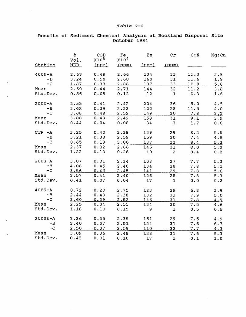
Table 2-2

Results of Sediment Chemical Analysis at Rockland Disposal site october 1984

% COD Fe Zn Cr C:N Mg:Ca Vol. X10 5 X10 4

station NED (ppm) (ppm) (ppm) (ppm)

400N-A 2.68 0.49 2.66 134 33 11.3 3.8 -B 3.24 0.50 2.60 160 31 11. 6 1.9 -C 1. 87 0.33 2.88 137 33 10.8 5.8

Mean 2.60 0.44 2.71 144 32 11. 2 3.8 std. Dev. 0.56 0.08 0.12 12 1 0.3 1.6

200N-A 2.55 0.41 2.42 204 36 8.0 4.5 -B 3.62 0.39 2.33 122 28 11. 5 4.0 -C 3.08 0.48 2.52 149 30 7.8 3.1

Mean 3.08 0.43 2.42 158 31 9.1 3.9 Std.Dev. 0.44 0.04 0.08 34 3 1.7 0.6

CTR -A 3.25 0.40 2.38 139 29 8.2 5.5 -B 3.21 0.38 2.59 159 30 7.4 4.9 -C 0.65 0.18 3.00 137 33 8.4 5.3

Mean 2.37 0.32 2.66 145 31 8.0 5.2 Std.Dev. 1. 22 0.10 0.26 10 2 0.4 0.2

200S-A 3.07 0.31 2.34 103 27 7.7 5.3 -B 4.08 0.45 2.40 134 28 7.8 5.1 -C 3.56 0.46 2.45 141 29 7.8 5.6

Mean 3.57 0.41 2.40 126 28 7.8 5.3 Std. Dev. 0.41 0.07 0.04 17 1 0.0 0.2

400S-A 0.72 0.20 2.75 123 29 6.8 3.9 -B 2.44 0.43 2.38 132 31 7.9 5.0 -C 3.60 0.39 2.52 146 31 7.8 4.9

Mean 2.25 0.34 2.55 134 30 7.5 4.6 Std.Dev. 1.18 0.10 0.15 9 1 0.5 0.5

2000E-A 3.36 0.35 2.35 151 29 7.5 4.9 -B 3.40 0.37 2.51 124 31 7.6 6.7 -C 2.50 0.37 2.59 110 32 7.7 4.3

Mean 3.09 0.36 2.48 128 31 7.6 5.3 Std.Dev. 0.42 0.01 0.10 17 1 0.1 1.0

station

400W-A -B -C

Mean std.Dev.

200W-A -B -C

Mean Std.Dev.

CTR -A -B -C

Mean Std.Dev.

200E-A -B -C

Mean Std.Dev.

400E-A -B -C

Mean Std.Dev.

2000E-A -B -C

Mean Std.Dev.

% Vol. NED

3.47 3.72 3.00 3.40 0.30

2.12 2.50 3.00 2.54 0.36

3.25 3.21 0.65 2.37 1. 22

2.82 3.18 3.94 3.31 0.47

4.10 3.11 4.06 3.76 0.46

3.66 3.40 2.50 3.19 0.50

Table 2-2 continued.

COD X10 5 (ppm)

0.56 0.60 0.55 0.57 0.02

0.31 0.36 0.37 0.35 0.03

0.40 0.38 0.18 0.32 0.10

0.35 0.37 0.40 0.37 0.02

0.42 0.38 0.44 0.41 0.02

0.35 0.37 0.37 0.36 0.01

Fe X10 4 (ppm)

2.23 2.47 2.11 2.27 0.15

2.25 2.24 2.30 2.26 0.03

2.38 2.59 3.00 2.66 0.26

2.40 2.36 2.38 2.38 0.02

2.81 2.49 2.53 2.61 0.14

2.35 2.51 2.59 2.48 0.10

Zn

(ppm)

148 156 130 145

11

130 138 123 130

6

139 159 137 145

10

200 146 116 154

35

145 134 140 140

4

151 124 110 128

17

- indicates no data available.

Cr C:N Mg:Ca

(ppm)

9.2 1.3 12.8 0.9 22.2 0.6 14.7 0.9 5.5 0.3

22 8.8 5.4 22 7.2 3.3 23 8.6 4.4 22 8.2 4.4

0 0.7 0.9

29 8.2 5.5 30 7.4 4.9 33 8.4 5.3 31 8.0 5.2

2 0.4 0.2

25 7.4 3.6 25 7.6 6.7 24 7.6 5.4 25 7.5 5.2

0 0.1 1.3

33 7.4 4.7 30 7.7 4.2 32 8.8 5.2 32 8.0 4.7

1 0.6 0.4

29 7.5 4.9 31 7.6 6.7 32 7.7 4.3 31 7.6 5.3

1 0.1 1.0

station

400NE-A -B -C

Mean Std.Dev.

200NE-A -B -C

Mean Std.Dev.

CTR -A -B -C

Mean Std.Dev.

200SW-A -B -C

Mean Std.Dev.

400SW-A -B -C

Mean Std.Dev.

2000E-A -B -C

Mean Std.Dev.

% Vol. NED

3.89 2.86 2.64 3.13 0.54

3.11 2.92 2.96 3.00 0.08

3.25 3.21 0.65 2.37 1. 22

3.38 2.28 2.82 2.83 0.45

3.82 3.82 4.07 3.90 0.12

3.66 3.40 2.50 3.19 0.50

Table 2-2 continued.

COD Xl0 5

(ppm)

0.43 0.41 0.51 0.45 0.04

0.39 0.47 0.42 0.43 0.03

0.40 0.38 0.18 0.32 0.10

0.57 0.39 0.51 0.49 0.07

0.49 0.61 0.72 0.61 0.09

0.35 0.37 0.37 0.36 0.01

Fe Xl0 4 (ppm)

0.13 2.57 1. 35 1. 22

1. 82 2.59 2.52 2.31 0.35

2.38 2.59 3.00 2.66 0.26

2.30 2.20 2.24 2.25 0.04

2.28 2.22 2.43 2.31 0.09

2.35 2.51 2.59 2.48 0.10

Zn

(ppm)

170 132 136 146

17

113 105 168 129

28

139 159 137 145

10

154 147 141 147

5

161 126 120 136

18

154 124 116 131

16

- indicates no data available.

Cr C:N Mg:Ca

(ppm)

33 7.1 32 8.7 106 32 7.0 13.6 32 7.6 59.8

0 0.8 46.2

30 7.5 31 7.4 5.9 32 7.7 6.1 31 7.5 6.0

1 0.1 0.1

29 8.2 5.5 30 7.4 4.9 33 8.4 5.3 31 8.0 5.2

2 0.4 0.2

8.5 4.2 8.2 2.8

31 7.8 4.1 31 8.2 3.7

0.3 0.6

31 8.0 3.6 31 7.5 4.5 32 7.3 5.8 31 7.6 4.6

0 0.3 0.9

29 7.5 4.9 31 7.6 6.7 32 7.7 4.3 31 7.6 5.3

1 0.1 1.0

station

400NW-A -B -C

Mean Std.Dev.

200NW-A -B -C

Mean Std.Dev.

CTR -A -B -C

Mean Std.Dev.

200SE-A -B -C

Mean Std.Dev.

400SE-A -B -C

Mean Std.Dev.

2000E-A -B -C

Mean Std.Dev.

Vol. NED

3.76 3.64 3.24 3.55 0.22

2.01 2.56 2.85 2.47 0.35

3.25 3.21 0.65 2.37 1. 22

3.27 3.75 3.26 3.43 0.23

3.02 2.22 3.78 3.01 0.64

3.66 3.40 2.50 3.19 0.50

Table 2-2 continued.

COD XI0 5

Ippm)

0.63 0.40 0.37 0.47 0.12

0.18 0.64 0.56 0.46 0.20

0.40 0.38 0.18 0.32 0.10

0.28 0.43 0.28 0.33 0.07

0.38 0.38 0.41 0.39 0.01

0.35 0.37 0.37 0.36 0.01

Fe Xl0 4

Ippm)

2.19 2.49 2.50 2.39 0.14

2.92 2.30 2.19 2.47 0.32

2.38 2.59 3.00 2.66 0.26

2.44 2.48 2.45 2.46 0.02

2.52 2.56 2.53 2.54 0.02

2.35 2.51 2.59 2.48 0.10

Zn

(ppm)

163 154 179 165

10

151 122 136 136

12

139 159 137 145

10

167 134 151 151

13

106 125 143 125

15

154 124 116 131

16

- indicates no data available.

Cr C:N Mg:Ca

(ppm)

30 7.3 6.2 29 7.8 7.1

7.4 . 6.1 30 7.5 6.5

1 0.2 0.4

27 1.3 28 8.4 2.5 29 11.3 0.8 28 9.9 1.5

1 1.4 0.7

29 8.2 5.5 30 7.4 4.9 33 8.4 5.3 31 8.0 5.2

2 0.4 0.2

31 7.8 3.4 31 7.4 4.3 30 7.6 4.5 31 7.6 4.1

0 0.2 0.5

30 7.2 5.1 31 6.8 4.8 30 8.1 4.0 30 7.4 4.6

0 0.5 0.5

29 7.5 4.9 31 7.6 6.7 32 7.7 4.3 31 7.6 5.3

1 0.1 1.0

Table 2-3

Results of the Bivariate Analysis of 3-HLP Current Meter Data Collected at Rockland at a Depth of 10m

21 May to 11 June 1985

FREiUEHCY DIS1RI'UTJQN 1.00 HOURLY DA1A SlAllON. RCKII 3HRLP SPMNING 51211.5 TO b/lI185 521 DATA POINTS

DIRECTION DEGREES

PERCENT MEAN !1M "AX STD. DEY

~ 1.5 4.8 5.4 5.0 4.2 3.b 1.9 1.2 1.2 1.0 .2

30- 10 .2 4.0 1.0 .1 .2 .0 .0 .0 .0 .0 .0

60- 90 1.0 4.4 1.2 .4 .0 .0 .0 .0 .0 .0 .0

IH20 1.2 2.5 1.5 .4 .2 .0 .0 .0 .0 .0 .0

120-150 1.0 3.b 2.5 .b .2 .0 .0 .0 .0 .0 .0

150-180

180-210

210-240

241)-270

270-300

300-330

1330-300!

SPEED

C~/S

.4 2.7 b.3 2.1 1.7 •• 1.0 .8 .2 .0 .0

.0 1.2 1.2 1.3 .b .4 .4 .2 .0 .0 .0

.2 .0 .2 .2 .0 .0 .0 ,0 ,0 .0 ,0

.4 .4 .2 .0 ,0 .0 .0 ,0 .0 .0 ,0

.0 .b .0 .0 .0 .0 .0 .0 .0 .0 .0

.2 .2 .4 .0 .2 .0 .0 .0 .0 .0 .0

.4 2.7 4.0 2.5 2.1 1.2 1.7 1.5 1.2 .4 .2

,......~-o.-:1';12 II 20 24 2. 32 36 40

8 12 Ib • H ~ D M 40 «

PERCENT I.l 27.1 23.8 13.8 10.2 6.0 5.0 3.6 2.5 1.3 .4 !'tEAM DIR Il9 120 151 1.H 1S4 101 111 1'111 H!U lUI ItI~

sra DEV f6 100 110 120 1413 US 145 HO U4 162 2313

SUl1IIARY STAllSms IIE~H SPEED I 1l.1b ':11/5 "AUIIUM a 413.11 CHIS "INlnUII" 1.:U CI1'$

SlANDARD OEYIAlION' 8.37 cm SKEiNESS' 1.09

IN A CDDRBIHAIE SYSlE' WHOSE Y AlIS IS POSITIONED .00 DEGREES CLDCkilSE FRO. TRUE HDRIH !'lEAN I CQItPOtlEHT ~ 2.19 [IUS STANDARD DEIJIAlION· 1.85 CI1'S SKEWNESS. ,13 /fUm r COtll'llNClI'f ~ ~.e8 e/Us SrANIUl{{O DlvIAT/DN ~ Jot.l101/5 Sr.EWNESS·.1I

SPEED SPEED SPEED

D!;!) Ib.OI 1.31 40.27

b.O 7.38 3.47 lUI

b.9

5.' 7.1

Fl L::J

.b

1.0

.b

b.42 1.77 14.55

7.31 1.81 II.lb

7.96 2.24 1'.3b

u.ss 2.01 32.'3

14.11 b.47 21.12

1.11 2.71 15.2b

5.1' 2.b5 1.77

5.29 1.98 5.'8

1.0 1.11 3.45 17.49

@!J 17.28 2.02 40.71

100.00

RANGE. 39.40 CK/S

•

1.24

4.01

3.18

3.lb

2.83

6.b3

6.22

4.84

3.38

3.47

5.15

9.00

"

Table 3-1

Estimates Of Material In Water Column After Disposal1

Maximum Time After

Low Tide (H:MM)3

Time After Suspended Estimate of Distance from Date

Volume2 Disposal Sediment4 % Material Disposal

21 May 1985 (1205m3 )

22 May 1985 (1454m3 )

24 May 1985 (2780m3 )5

3:43

0:27

2:46

(min)

0 15 37

0 40

100

0 50

135

(mgll)

950 40

9

1100 22 12

1420 110

13

In Water Column Point

15-17 12-13 300

5.3-6.1 500

25-38 1.9-2.2 350 1.4-1. 6 500

67-77 37-42 700

2.3-2.7 1700

1 Assumes the bulk density of dredged material in scow = 1.4 to 1.6 g/cm3 . 2 Based on scow log volumes estimated by draft of scow. 3 Maximum flood current velocities occur approximately three hours after Low Tide. 4 Average concentrations over areas indicated in Figures 3-2, 3-4, and 3-6. 5 Two scows dumped together.

* u. S. GOVERNMENT PRINTING OFFICE: 1988--500-017--60051

(m)