Displaced Capital: A Study of Aerospace Plant Closings

958

[Journal of Political Economy, 2001, vol. 109, no. 5]� 2001 by The University of Chicago. All rights reserved. 0022-3808/2001/10905-0002$02.50

Displaced Capital: A Study of Aerospace PlantClosings

Valerie A. RameyUniversity of California, San Diego and National Bureau of Economic Research

Matthew D. ShapiroUniversity of Michigan and National Bureau of Economic Research

Using equipment-level data from aerospace plants that closed duringthe 1990s, this paper studies the process of moving installed physicalcapital to a new use. The analysis yields three results that suggestsignificant sectoral specificity of physical capital and substantial costsof redeploying the capital. First, other aerospace companies areoverrepresented among buyers of the used capital relative to theirrepresentation in the market for new investment goods. Second, evenafter age-related depreciation is taken into account, capital sells fora substantial discount relative to replacement cost; the more special-ized the type of capital, the greater the discount. Yet, capital sold toother aerospace firms fetches a higher price than capital sold to in-dustry outsiders. Finally, the process of winding down operations andselling the equipment takes several years.

We are greatly indebted to the managers, auctioneers, and machine tool salesmen whoprovided us with data and valuable insights. We have also benefited from the helpfulcomments of an anonymous referee as well as seminar participants at the University ofCalifornia, San Diego, University of Michigan, Massachusetts Institute of Technology, Uni-versity of Texas at Austin, University of California, Riverside, University of California, SantaBarbara, Northwestern, Rand, Princeton, Wharton, Indiana, Hebrew University, Tel Aviv,Haifa, Stanford, Yale, the Federal Reserve Bank of New York, and the National Bureau ofEconomic Research’s Economic Fluctuations and Growth and Sloan Project conferences.We both gratefully acknowledge financial support from Sloan Foundation fellowships,funding from the Alfred P. Sloan Foundation via a grant to the Industrial Technology andProductivity Project of the National Bureau of Economic Research, and National ScienceFoundation grant SBR-9617437. We thank Marina Anastasia Vladimirovna and ElizabethVega for very capable research assistance. We have agreed to keep confidential the identityof the companies and the source data on which this study is based.

displaced capital 959

I. Introduction

Changes in technology, the demand for output, or factor prices canlead to the displacement of capital from its original use. The efficiencywith which that capital can be redeployed to other firms and sectors isan important determinant of the economy’s speed of transition after ashock. It is also an important element in firms’ initial investment de-cisions. Recent empirical work has provided indirect evidence of costlyadjustment of capital by showing that investment behavior is consistentwith the presence of costly disinvestment. There is little direct evidence,however, on the sectoral specificity of capital or the speed with whichcapital can be redeployed.

We seek to fill this gap by collecting and analyzing data in order toshed light on capital specificity and the efficiency of resale markets inredeploying displaced capital. To this end, we collected confidentialinformation from auctions of equipment from three large southernCalifornia aerospace plants that discontinued operations. We then usedinformation on sales prices and the characteristics of buyers to deter-mine the extent of capital specificity for this particular industry. We shallargue below that the aerospace industry is particularly interesting be-cause it has undergone significant, exogenous downsizing.

Our findings suggest that much capital is very specialized by sectorand that reallocating capital across sectors entails substantial costs. Theestimated average market value of equipment in our sample is 28 centsper dollar of replacement cost. Even machine tools, which typically havegood resale markets, sell for less than 40 percent of replacement cost.Types of capital that we identify as being more specialized sell at a greaterdiscount. Yet, capital that sells to other aerospace firms sells at a smallerdiscount than capital that sells to outsiders. This loss of value is not theonly cost of displacement. The process of winding down operationsbefore selling the capital results in significant periods of low utilizationbefore the capital is finally sold. Moreover, the process of selling alsotakes substantial time, so there is a time cost of reallocation. Neverthe-less, the assumption of zero fungibility of capital is also far from true.We find that capital is sold to firms in a wide range of sectors as wellas in far-flung geographical locations.

The estimates of this paper should prove useful for at least two dif-ferent lines of research. First, by providing direct evidence on the costsof reversing investment decisions, this paper contributes to the mac-roeconomics literature on the role of costly reversibility at the firm level

960 journal of political economy

and in the economy as a whole.1 Theoretical models of firm behavior(e.g., Abel and Eberly 1994; Dixit and Pindyck 1994) make predictionsabout how these kinds of adjustment costs affect the timing and mag-nitude of investment. Other studies, such as Veracierto (1997) and Ra-mey and Shapiro (1998a), consider the role of costly reversibility indynamic general equilibrium models. Our direct estimates of the lossof value for reversing an investment can be used to calibrate the the-oretical models and to generate predictions about how uncertaintymight delay investment. Moreover, our evidence concerning the delaysin the process of disinvestment provides direct support for some of thepredictions of these models.

A second line of research to which our results relate is the literatureon depreciation measurement. A by-product of our study is a set ofestimates of annual depreciation rates of equipment. The depreciationmeasurement studies, such as those by Hall (1971), Hulten and Wykoff(1981), Bond (1982), Cockburn and Frank (1992), and Oliner (1996),also employ sales of used assets to infer the productive value of assets.2

Those studies do not have information on the original purchase priceof equipment, so they use hedonic techniques to infer depreciationrates. Even though we use a different type of data and technique, ourdepreciation estimates are very similar to the estimates from thatliterature.

The remainder of the paper is organized as follows. Section II dis-cusses the role of specificity in the marketing of used equipment. SectionIII describes the data that we have collected. Section IV presents theresults on to whom and how the equipment was sold. These resultsprovide some evidence on the extent of specificity of the equipment.Section V presents a regression model based on a subset of the equip-ment in which we observe the original cost. We present estimates of thediscount from replacement cost from selling the equipment and theway in which the discount varies by the industry of the buyer or modeof sale. These estimates provide quantitative evidence of the value ofspecificity. As a by-product, the regression model produces estimates onthe rate of depreciation. In the last part of this section, we also discusshow the specificity of capital in aerospace compares to other industries.Section VI provides evidence on the time cost of the process of real-location. Section VII relates our findings to the literature on displacedworkers and offers our conclusions.

1 Indirect empirical evidence on the importance of adjustment costs is provided byCaballero and Engel (1999), who use industry-level data; by Abel and Eberly (1996), whouse firm-level data; and by Caballero, Engel, and Haltiwanger (1995), who use plant-leveldata.

2 See Jorgenson (1996) and Fraumeni (1997) for excellent surveys of empirical studiesof depreciation.


II. The Market for Used Capital: The Importance of Specificityand Market Thinness

On the basis of discussions with auctioneers, industry insiders, and ma-chine tool manufacturers, we consider the following characterization tobe a plausible depiction of the market for used capital. Most capital isspecialized by industry, so that used capital typically has greater valueinside the industry than outside the industry. Even within an industry,though, capital from one firm may not be a perfect match for anotherfirm. Thin markets and costly search complicate the process of findingbuyers whose needs best match the capital’s characteristics. The cost ofsearch includes not only monetary costs but also the time it takes tofind good matches within the industry. As a result, firms will not searchexhaustively for the best match for all their pieces of capital. Firms withhigh time discount factors may resort to “fire sales,” resulting in signif-icantly inferior matches and the reallocation of capital to lower-valueuses. This story contains two key elements: sectoral specificity and marketthinness. Sectoral specificity can arise when each piece of capital has acertain set of physical characteristics. When new capital is built for saleto a specific sector, it will have the best match of features for that sector.3

Despite the specificity of these characteristics, capital can be reallocatedacross sectors. The key is that only some of the characteristics of aparticular piece of capital will have value in another sector.

We illustrate this idea with three examples from the aerospace in-dustry and one example from the educational services industry. Thefirst example of specificity is a wind tunnel. A low-speed wind tunnel,capable of producing winds from 10 to 270 miles per hour, was sold toa company outside of the aerospace industry (San Diego Union-Tribune,October 23, 1994). This company rents the wind tunnel for $900 anhour to businesses such as bicycle helmet designers and architects whowish to gauge air flows between buildings. Most of the users requireonly low wind speeds and do not value the fact that the tunnel canproduce wind speeds of 270 miles per hour. Thus a key characteristicof this wind tunnel—high wind speeds—has no value outside ofaerospace.

A second example is the machine tools used by aerospace manufac-turers. The resale market for machine tools is one of the thickest marketsfor used capital equipment. Nevertheless, there is reason to believe thatmany of the machine tools used by aerospace industries have features

3 Firms might design or purchase equipment with ex post flexibility in mind (see Stigler1939; Fuss and McFadden 1978). (In a visit to an automobile assembly plant, we were toldthat the firm paid an extra 10 or 15 percent to purchase machine tools that could beeasily reconfigured.) Even if this flexibility is built in ex ante, the capital will lose somevalue if the flexibility needs to be employed ex post, except in the unlikely event that thedesign made the capital perfectly flexible.


that are substantially less valuable for other industries. As explained tous by a leading machine tool manufacturer, the manufacture of aero-space goods involves much larger pieces of metal than the manufactureof most other goods. As a result, machine tools for aerospace are muchbigger and must have significantly higher horsepower than the averagemachine tool. Consider the example of dual and triple gantry profilers,which constitute some of the equipment in our sample. These piecesof machinery, which can move large portions of fuselage or wing to thecutting area, are 75 feet or more in length and weigh several tons.4 Theyhave limited use outside of aerospace.

A third example consists of the instruments used by aerospace man-ufacturers. Because precision is crucial in the manufacture of aerospaceparts, the extra precision built into the tools and instruments has ahigher value in aerospace than outside aerospace. For example, onecoordinate-measuring machine in our sample could test the accuracyof parts at tolerances of less than 0.0001 of an inch. This piece ofmachinery sold at a substantial discount to a machinery dealer.

Our final example, from outside the aerospace industry, consists ofthe building currently housing the Department of Economics at theUniversity of California at Riverside. This building is a converted motel,so it is an example of a piece of capital that moved from standardindustrial classification (SIC) code 70 (hotels) to SIC code 82 (educa-tional services). Each office has a bathroom complete with shower, andthe department has its own swimming pool. While these features havesignificant value for lodgers and thus affect the value of services offeredby a motel, one may question whether these amenities contribute tothe productivity of research or teaching of the economics faculty.

These examples show how capital can consist of a bundle of special-ized features. Although capital from one industry can be used in anotherindustry in many cases, many of the features will have little or no valueto the second industry. Thus the value of the capital decreases when itcrosses industries.5

The second key element in our story is thin markets. We believe thatthin markets for used capital are an important impediment to the ef-ficient reallocation of capital. Our discussions with professional liqui-dators and auctioneers suggested several transaction costs in the real-location of capital. Finding buyers whose needs closely match thecharacteristics of the equipment is a costly and time-consuming process.

4 An article on the first page of the October 21, 1996, Wall Street Journal discusses thecase of a dual gantry profiler, purchased new for $5 million and sold for $2,500 at auction.Our empirical results show that this case is not unusual.

5 Bond (1983) considers a different type of heterogeneity in order to explain why thereis substantial trade in used assets. He argues that differences in firms’ factor prices andcapital utilization lead to different valuations of new vs. used assets.


The sale of the equipment must be advertised, and the process of in-spection, negotiation, and capital budgeting can be lengthy. On theother hand, the firm can hold a public auction, which takes place overa couple of days, but it may result in inferior matches between capitalcharacteristics and buyers’ needs. Thus firms face a trade-off betweenselling early at a low price and searching at length for high-valuationbuyers. Ramey and Shapiro (1998b) provide a model taking into accountspecificity and market thinness that analyzes this trade-off and showshow firms might endogenously switch between different modes of sale.

The combination of capital specificity and market thinness can serveto add costs to the reallocation of capital across firms and industries.We use these theoretical considerations to motivate our econometricspecification in Section V. By examining how the value of reallocatedcapital varies by who purchased it and by the mode of the sale, we canquantify the equilibrium consequences of capital specificity and marketthinness.

III. Data Description

Our data consist of information on capital sales from southern Californiaplants belonging to three large aerospace companies. The aerospaceindustry underwent enormous downsizing and restructuring in the1990s owing to the end of the Cold War. The exogeneity and large sizeof the shock driving the decision to reallocate the capital essentiallyeliminate concerns about the endogeneity of demand for the factories’output and about nonrandom selection of pieces of equipment.

Variations in defense spending represent major shifts in total demandfor aerospace goods. In 1987, shipments to the Department of Defenseaccounted for 60 percent of total shipments of aircraft (SIC 372) andmissiles and space vehicles (SIC 376).6 Furthermore, Defense Depart-ment demand is highly variable. Figure 1 shows real defense purchasesof aerospace equipment over time. From 1977 to 1988, real purchasesrose 225 percent. From 1988 to 1995, real purchases reversed them-selves, declining back to their 1977 levels.

We study three of the many plants that closed in the 1990s. All threeplants, which were owned by different firms, were important manufac-turers of military or commercial airplanes, as well as missiles. Two ofthe plants were over 40 years old, and the third was about 20 years old.At the time we obtained the data, the third plant was in the process ofslowly paring down operations but had not completely closed. In allcases, after several years of declining production and employment, the

6 Shipments to the National Aeronautics and Space Administration accounted for an-other 6 percent of total shipments of aerospace equipment.


Fig. 1.—Defense purchases of aerospace equipment

firms decided to discontinue operations. The decisions on all theseplants, however, came several years after the majority of plant closures,so none of these plants was a marginal plant.

Two of the firms held their sales through the same liquidation andauction company. Plant 1 sold equipment through private negotiation(“private liquidation sale”) over the space of four months and then soldthe remaining equipment at a public auction that took approximatelyone week. Plant 2 held no liquidation sale but held a series of publicauctions over the year and a half that it was winding down operations.Plant 3 held a public auction through another company. All the publicauctions were conducted as English auctions. According to the auc-tioneers, most of the larger items had multiple bidders. The total pro-ceeds from the sales were $18.7 million. Over 1,000 buyers purchasedequipment. Three times as many buyers attended the auctions.

A significant part of the equipment sold was machine tools, such asmilling machines, jig mills, and lathes. These are the standard metal-cutting and metal-forming equipment used in manufacturing aircraftparts. But there was also a great variety of other goods sold, such asforklifts, cranes, generators, vibratory finishers, drill bits, and even caf-eteria chairs. Thus our data cover a fairly wide span of equipment.

It is interesting to note that the manufacturers did not sell any build-ings.7 Not selling buildings is not unusual for plant closings involving

7 We do not yet know the outcome for the buildings of plant 3.


plants that are more than 25 years old. Many have found that the costof bringing the plants up to current environmental standards (e.g.,removing asbestos) is greater than the potential sales price, so theysimply raze the buildings.

For every item sold in the liquidation sale and public auctions (over20,000 lots), we obtained information on the complete equipment de-scription, the sales price, and the identity of the buyer. Using businessdirectories, as well as direct phone calls to buyers, we assigned buyersto a four-digit SIC industry. Buyers whose industries we could not identifyaccounted for less than 4 percent of total sales. The industry informationallowed us to track the reallocation of the equipment to variousindustries.

The most useful data are the information we obtained from plant 1for an important subset of its equipment. In addition to the informationdiscussed above, the selling company provided us with information onthe original purchase year and transaction price as well as the year andcost of any refabrications or rebuilds for almost all the pieces of equip-ment that sold for $10,000 or more each. We were able to obtain in-formation for 129 lots that accounted for $7.1 million of sales. Hence,though these data are only a small fraction of the number of sales, theyaccount for over half of the value. With this information, we can com-pare the resale price to the original purchase price and hence estimatethe discounts.

The richness of the data set we have collected overcomes many ofthe criticisms that have been made of studies of sales of used equipment.For example, several features of the data suggest that there should notbe a significant “lemons problem.” First, the tremendous amount ofdownsizing that occurred meant that the plants that closed were notmarginal plants. Second, we know that the downsizing was due to ex-ogenous demand shifts, not to technological problems in manufacturingaerospace goods. Third, the fact that the plants sold everything theyowned means that there is no selection bias in the equipment that wassold.

A second criticism that our data set overcomes is concerns about theprice data. Wykoff (1970) questioned his estimates of the steep declinein value in automobiles during the first year because he was forced tocompare the price of one-year-old cars to the list price of new cars. Ifthe actual transactions price features discounts off the list price, thenthe depreciation estimates can be biased. In our case, we have both theactual price that plant 1 paid for the equipment when new and theactual price it received when it resold the equipment. Thus our estimatesare based on actual transactions prices.

We conduct three types of analyses of the data that shed light oncapital mobility. In Section IV, we compute the distribution of sales of


equipment across industries. The extent to which the sales are moreconcentrated in aerospace or manufacturing relative to the aggregategives an indication of the specialization of equipment. We also distin-guish the distribution of sales according to whether the good was soldthrough private negotiation or public auction. In Section V, we shalluse the subset of sales for which we have original purchase prices toestimate a model of economic depreciation. We shall estimate depre-ciation rates and compare them to others in the literature. In SectionVI, we shall discuss the time lags that were involved in the sale of capital.

IV. Who Bought the Capital and How Was It Sold?

Before we present our results on the sectoral flows of capital from thethree plants, it is useful to give an indication of the aggregate demandsfor equipment for comparison purposes. The Annual Capital Expen-ditures Survey reports that in 1993 the aerospace industry representedjust 0.78 percent of total private expenditures on producers’ durableequipment and just 2.5 percent of manufacturing expenditures. Al-though the aerospace industry is more heavily concentrated in Califor-nia, it is unlikely that its fraction of investment was much higher, giventhe downsizing that was occurring. The manufacturing sector as a wholeaccounted for 32 percent of all investment in producers’ durable equip-ment in 1993.

Against this backdrop, we calculate the flow across sectors of equip-ment from our data. To our knowledge, this is the first study to trackcapital equipment as it flows out of a shrinking industry. Using everyitem sold, we calculated the fraction of goods that went to each industry,by both the value of sales and the number of buyers. Tables 1, 2, and3 present the distribution of sales of equipment by buyers’ industriesand locations. Table 1 shows the results for all types of sales combined,table 2 shows the results for the private liquidation sales, and table 3shows the results for the public auctions.

Table 1 shows one of the central findings of our paper. The equipmentis sold disproportionately to buyers within aerospace. A quarter of equip-ment stays within the sector, 30 times the share of aerospace in overallequipment investment. Nonetheless, three-quarters of the equipmentleaves the sector. Hence, specificity is important but not absolute.

Table 1 also shows several other sectors that were major buyers. Ma-chinery dealers bought 23 percent of the equipment. We are not ableto track this equipment to its final destination. It is likely that some ofthis equipment was resold to aerospace manufacturers. The other im-portant set of buyers was firms in the fabricated metals and machineryindustries, who together bought 28 percent of the equipment. Many ofthese industries use the types of machine tools used by aircraft manu-


TABLE 1Distribution of Sales by Industry and Region: All Sales Included

Industry Percentage of Sales ValuePercentage of Buyers

(Np1,207)

Aerospace (SIC 372, 376) 24.2 5.2Other transportation

equipment 1.6 1.7Fabricated metals and

machinery 27.8 25.9Other manufacturing 4.0 6.1Machinery dealers 22.8 14.3Construction 2.5 3.4Transportation and pub-

lic utilities 1.1 1.3Retail trade 2.8 2.9Services 5.0 7.9Individuals 3.9 12.3Other .6 .3Unknown 3.7 18.6Region:

California 63.8 89.2Rest of United States 32.3 9.9Foreign 4.0 .8

Total sales value $18,723,607

Note.—Table includes data from plants 1, 2, and 3.

facturers. Manufacturing as a whole accounted for 58 percent of sales,which is about twice its share in aggregate equipment investment.

We also note the geographic dispersion of sales at the bottom of thetable. Over one-third of the equipment was sold to buyers outside ofCalifornia, and 4 percent was sold to buyers from outside the UnitedStates. This calculation of the percentage sold to foreigners is probablyan underestimate. Many sales to foreign countries go through U.S. deal-ers or through individuals who serve as agents.8

The data show that capital is not absolutely stationary since more thanone-third of it left California. Yet, that California accounted for a muchlarger share of sales than it does in the aggregate investment data showsthat there are costs to geographic mobility. Some of the equipment,such as the double gantry profilers, weighs several tons, so transportcosts are nontrivial. In any case, just as with industry, geographical spec-ificity is substantial, but not absolute.

Tables 2 and 3 show that there is a significant difference in the buyersthrough private liquidation and public auction. Table 2 shows that two-thirds of the sales value from the liquidation sale went to other aerospace

8 According to some auctioneers, a significant part of the equipment sold at aerospaceauctions was sold to foreign manufacturers in China and India. China obtained someweapons-manufacturing equipment illegally through individuals who attended defenseindustry auctions (Wall Street Journal, October 21, 1996, p. A1).


TABLE 2Distribution of Sales by Industry and Region: Private Liquidation Sales


(Np22)


equipment 0 0Fabricated metals and

machinery 10.1 22.7Other manufacturing .7 4.5Machinery dealers 22.4 36.4Construction 0 0Transportation and pub-

lic utilities 0 0Retail trade 0 0Services 0 0Individuals 0 0Other 0 0Unknown 0 0Region:

California 36.4 36.4Rest of United States 54.6 59.0Foreign 9.0 4.6


Note.—Table includes data from plant 1.

firms, whereas table 3 shows that only 10 percent of the public auctionsales went to aerospace firms. The characterization of markets for usedcapital discussed in Section II is helpful for interpreting these results.If aerospace firms have higher valuations for the equipment but areharder to locate because of thin market effects, the selling firms mustspend time and effort seeking out other aerospace firms. Thus we wouldexpect most of the private liquidation sales to go to other aerospacefirms. When the expected return from this process becomes low enough,the firm sells all remaining units at a public auction. Most of the salesat public auction are made to industry outsiders. Firms that cannotafford to wait during the search process sell all their equipment at publicauction.

We can also explain why some plants had private liquidation sales andothers did not. Plant 1 had a private liquidation sale before its publicauction, whereas plant 2 did not. Plant 3 had an initial public auction(from which our data for the plant are taken) but planned to have aliquidation sale later as production decreased. At the time of its closing,plant 1 was owned by a firm that was cash rich. In contrast, at the timeof its closing, plant 2 was owned by a firm that was heavily indebtedand had low bond ratings. Plant 3 was also more heavily indebted thanplant 1. On the basis of these factors, one would expect the time discountrate of the owner of plant 1 to be much lower than those of the owners


TABLE 3Distribution of Sales by Industry and Region: Public Auctions


(Np1,185)


equipment 2.2 1.7Fabricated metals and

machinery 33.7 26.0Other manufacturing 5.1 6.2Machinery dealers 22.9 13.9Construction 3.4 3.5Transportation and pub-

lic utilities 1.5 1.4Retail trade 3.8 3.0Services 6.7 8.0Individuals 5.2 12.6Other .8 .3Unknown 4.9 18.9Region:

California 72.9 90.2Rest of United States 24.8 9.0Foreign 2.3 .8


Note.—Table includes data from plants 1, 2, and 3.

of plants 2 and 3. Thus these two plants would be expected to spendless time searching for other buyers inside the industry. This appearsto be exactly what happened in plant 2. Only 4.6 percent of plant 2’ssales went to aerospace buyers. In contrast, 32 percent of the sales fromplant 1 went to aerospace buyers. Since the plants appear to have similarequipment, we attribute the difference in the pattern in sales to theimpatience of the firms rather than to differences in the quality ofpotential matches to buyers within the industry.

These results are consistent with Pulvino’s (1998) findings for airlines.He found that financially constrained airlines receive lower prices thanunconstrained airlines when selling used aircraft. Furthermore, also con-sistent with our results, he found that financially constrained airlinesare more likely to sell their aircraft to a financial institution.

V. Estimates of Discounts and Economic Depreciation

A. Overview

In this section we use the subset of equipment from plant 1, for whichwe have data on original purchase prices, to obtain estimates of the lossof value suffered by capital sold as part of the consolidation and down-sizing of an industry. We begin with a summary of the data and a dis-cussion of depreciation estimates from other studies. We then estimate


several versions of a model of economic depreciation. Three main resultsemerge from the estimation: (1) equipment sold for significant dis-counts relative to the estimated replacement cost, (2) more specializedequipment sold for a higher discount, and (3) equipment bought byother aerospace firms or through the private liquidation sale sold fora higher premium.

As discussed in Section III, this subset of data consists of 129 lots witha total sales value of $7.1 million. To put the data on a current-costbasis, we reflate the original acquisition cost plus the cost of subsequentinvestment for rebuilds using implicit deflators for investment goods.9

In theory, these indexes should measure the change in price whenquality is held constant, so the reflated values represent replacementcost.10

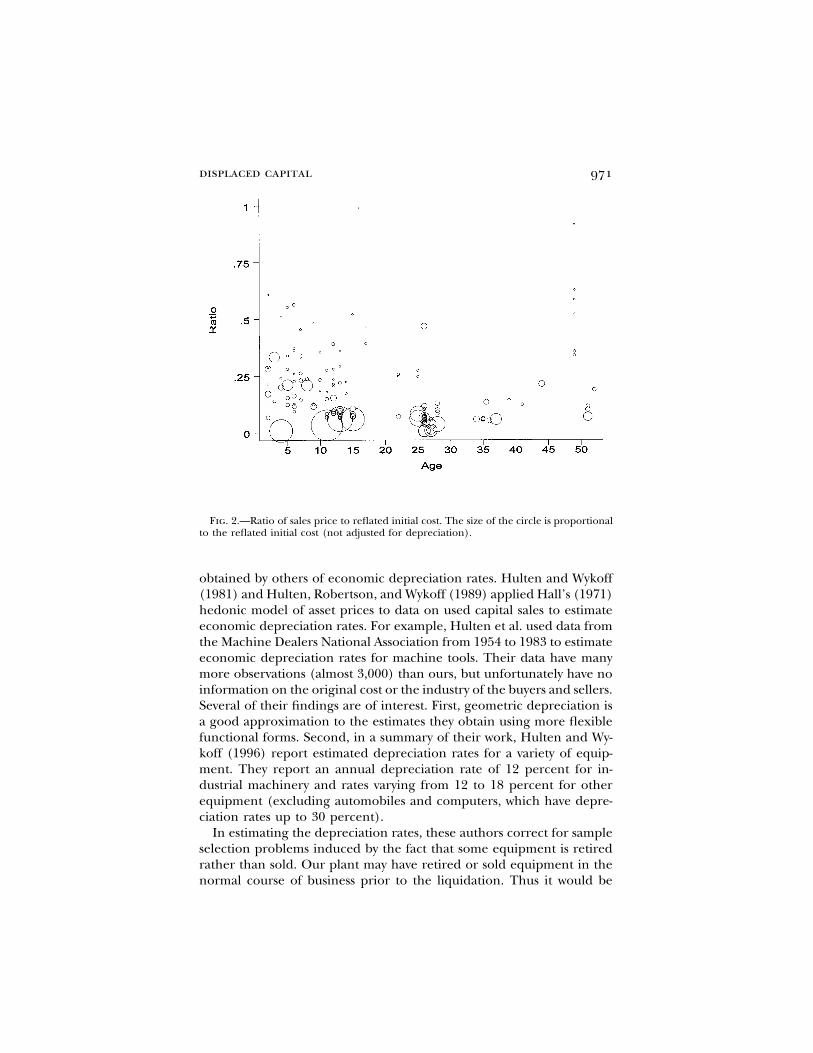
Figure 2 shows a plot of the ratio of the sales price to the reflatedoriginal acquisition cost against age. The figure shows the raw data oninitial purchase cost except for the adjustment for price change. Insubsequent analysis, we shall take into account depreciation and re-builds. The size of the circle is proportional to the reflated original cost.Several features stand out in the data. First, it is clear that there wereseveral large items with ages up to 15 years that suffered huge declinesin value. Second, some of the equipment that was nearly 50 years oldsold for a large fraction of its original purchase price. We double-checked these data to make sure they were not errors. We were toldthat there were certain types of machinery manufactured 50 years agothat were used only by aircraft manufacturers at the time. Later, however,other manufacturers started using this type of machinery, and sincethese exact types are no longer manufactured, many non–aircraft man-ufacturers are willing to pay a high premium to acquire it. There is alsosignificant selectivity in these data since our sample excludes previouslyretired equipment.

Before we estimate rates of depreciation, it is useful to review estimates

9 We are not revealing the price year of the auction to protect the confidentiality of thecompany. We reflate the acquisition cost by multiplying the historical cost by the ratio ofthe deflator in the year of the auction to the year of the purchase. We calculate the implicitdeflator as the ratio of historical cost to the chain-weighted quantity index using theinvestment series from the Bureau of Economic Analysis’s (BEA) capital stock data. Weuse the deflator for investment in metalworking machinery for the machine tools andsimilar equipment, the instruments investment deflator for the instruments, the deflatorfor investment in computers for computers, the price deflator for turbines for a generator,the deflator for construction tractors for gas-driven forklifts, and the deflator for invest-ment in industrial equipment for the remaining items.

10 Of course, price indexes can systematically miss changes in quality and therefore growtoo fast or too slow. According to Gordon’s (1990) estimates, Bureau of Labor Statisticsprice indexes miss quality improvements at the rate of roughly 1 percent per year. If therate of omitted quality change is roughly constant per year, it will lead us to overstate theestimated rate of depreciation.


Fig. 2.—Ratio of sales price to reflated initial cost. The size of the circle is proportionalto the reflated initial cost (not adjusted for depreciation).

obtained by others of economic depreciation rates. Hulten and Wykoff(1981) and Hulten, Robertson, and Wykoff (1989) applied Hall’s (1971)hedonic model of asset prices to data on used capital sales to estimateeconomic depreciation rates. For example, Hulten et al. used data fromthe Machine Dealers National Association from 1954 to 1983 to estimateeconomic depreciation rates for machine tools. Their data have manymore observations (almost 3,000) than ours, but unfortunately have noinformation on the original cost or the industry of the buyers and sellers.Several of their findings are of interest. First, geometric depreciation isa good approximation to the estimates they obtain using more flexiblefunctional forms. Second, in a summary of their work, Hulten and Wy-koff (1996) report estimated depreciation rates for a variety of equip-ment. They report an annual depreciation rate of 12 percent for in-dustrial machinery and rates varying from 12 to 18 percent for otherequipment (excluding automobiles and computers, which have depre-ciation rates up to 30 percent).

In estimating the depreciation rates, these authors correct for sampleselection problems induced by the fact that some equipment is retiredrather than sold. Our plant may have retired or sold equipment in thenormal course of business prior to the liquidation. Thus it would be


correct to make comparisons with estimates from other studies that arenot corrected for sample selectivity. According to Oliner (1996), Hultenet al.’s (1989) parameter estimates imply an unadjusted annual depre-ciation rate of 4.97 percent for a 12-year-old milling machine. Olinerhimself surveyed machinery dealers in the mid 1980s and estimated adepreciation rate of 3.5 percent for the group of machine tools still inoperation. Beidleman (1976) estimated a geometric depreciation rateof 7.48 percent for unretired equipment. Thus the relevant estimatesfor our comparison range from 3.5 to 7.5 percent.11

Finally, it is important to bear in mind that because we examine theliquidation of an entire factory, our data do not suffer from the selectionproblem of equipment that is kept in service versus equipment that isdisposed of (whether through retirement or sale).

B. Depreciation by Type of Equipment and the Value of Rebuilds

We begin by examining the age-related depreciation structure of theequipment and the returns on different categories of equipment. Weestimate the following model that relates the sales price to the replace-ment cost of capital and the replacement cost of capital to age andother characteristics. Equation (1) relates the sales prices of lot i, Si, tothe current-dollar (reflated), depreciated acquisition cost of initial in-vestments in the lot, Ki. Equation (2) defines Ki as a function of thecurrent-dollar investment Iiv. These equations are as follows:

S p c � (1 � a � g) 7 K � e (1)i 0 m r i i

and

2K p I 7 exp [�(d 7 age � d 7 age )]. (2)�i iv 1 iv 2 ivv

Let us explain in detail the parameterizations of these equations. (Table4 summarizes the notation.) Equation (2) is the standard definition ofthe net capital stock from depreciated, current-dollar investment flowswith several modifications. First, we need to sum over the items in thelots, indexed by v. For most lots, there is only one item, but for severalthere are two. Second, we strongly reject that depreciation is geometricin the age of the equipment, so we include a quadratic as well to capture

11 The BEA uses estimates based on the work of Hulten and Wykoff for its new data onthe capital stock (see Fraumeni 1997). Since the BEA uses a perpetual inventory of in-vestment with no systematic data on retirements, the appropriate depreciation rate for itscalculation does take into account the fact that some of the past investment flows are nolonger in service. Since our data exclude previously retired equipment, we estimate a lowerrate of depreciation than would be appropriate for the BEA’s calculation.


TABLE 4Notation Used in Equations (1), (2), (1′), and (1′′)

Variable Definition

Indices:i Index for lotsv Index for investments (within a single

lot)m Index for types of equipment

Parameters to be estimated:c0 Constant termam Discount on replacement cost of capital

of machinery type mgr Discount on rebuilt equipmentd1 Depreciation parameter on aged2 Depreciation parameter on the square of

agelaero Premium for goods sold to aerospace

buyerslliq Premium for goods sold at the private li-

quidation saleVariables:

Si Price at which lot i sold, in thousands ofdollars

Ki Estimated replacement cost, in thousandsof dollars

ei Error termIiv Investment expenditure v on lot i, re-

flated cost in thousands of dollarsAgeiv Years since vth investment on lot i

the nonconstancy of the depreciation rate. The coefficients d parame-terize the depreciation rate.

We substitute the definition (2) into equation (1), so we estimate asingle equation with a single error term ei. With gr and am equal to zero,equation (1) provides an estimate of the depreciation rate parametersfrom (2), so all loss in value of initial investment is related to age. Akey finding of this paper, however, is that not all loss of value is relatedto age. Hence, we introduce the parameters am and gr to capture dis-counts not related to age. The m subscript on a indexes type of equip-ment. We want to examine whether the discounts or premia vary by howspecialized the types of equipment are. (To avoid a lot of dummy var-iables in the notation, we use the following convention: If the lot con-tains equipment type m, am is nonzero; otherwise it is zero. We usesimilar notation for the other subscripted parameters.)

Some of the equipment was rebuilt. The parameter gr allows theselots to sell at a premium or discount. (Again, for lots that haveg p 0r

no rebuilds.) There are a number of ways that we could capture theeffect of rebuilds. In the Appendix, we explore various possibilities,including the expenditure on rebuilds explicitly in equation (2). We


find that the parsimonious specification of equation (1) is supportedby the data, so we use it in all the main results.

The error term e in equation (1) arises from different preferencesfor machinery features, different outcomes in the search process, andidiosyncratic differences in the rate of physical depreciation, all of whichare assumed to be independent of the original purchase price. Theconstant term is included to ensure a mean zero error term.

An important result is the extent to which the discount or premiuma varies by type of equipment m. In defining the types of equipment,we aimed to group similar equipment within type and highlight thespecialization of the equipment across types. We classified the equip-ment into the following six categories (N denotes the number of lotsin each category): machine tools ( ), bridge and gantry-type pro-N p 99filers ( ), instruments and measuring devices ( ), forklift-typeN p 7 N p 7equipment ( ), miscellaneous equipment ( ), and structuralN p 6 N p 8equipment ( ). Machine tools are the largest category and rep-N p 2resent a variety of milling machines, grinders, and other similar typesof equipment. We could not find any meaningful way to break thiscategory up any further.

The other groups contain much smaller numbers of items, althoughin some cases they represent significant amounts of revenue. Althoughprofilers are technically machine tools, we classified them as a separategroup. Recall that profilers are relatively specialized to aerospace be-cause they contain large gantry systems for moving large pieces of metal.Similarly, we put instruments in a separate category in case these itemsalso have some specificity to aerospace. The forklifts category representsthe most general capital of any in our subsample, containing forkliftsand electric loaders.12 Even these items were somewhat specialized inthat they were large enough to be able to move large parts of a fuselage.Miscellaneous equipment contains items such as ovens, vibratory finish-ers, and computers.

The final category, structural equipment, consists of only two verylarge, complex, and expensive items that required costly disassemblyand reassembly in order to be sold. Initial estimation showed that thetwo structural pieces of equipment noticeably lowered the exponentialdepreciation estimates, even after we allowed for a different discounta. These two lots are influential observations because of their very highinitial cost and very high discount. We do not believe that they add anyreal information on age-related depreciation because there is hetero-geneity between the two items within this category. Nor do they provideinformation for the later analysis by buyer and mode of sale because

12 Recall that this sample for the regressions contains only items that sold for $10,000or more. Thus the items such as cafeteria chairs are not in the sample.


TABLE 5Estimates of Depreciation Rates and Discounts by Type of Equipment

Parameter and VariableQuadratic

(1)Geometric

(2)

c0: Constant 1.764 (2.404) 4.132 (2.496)d1: Age .090 (.014) .051 (.0072)d2: Age2 �.0013 (.0003) 0am:

Discount on machine tools .629 (.048) .698 (.039)Discount on instruments .631 (.072) .739 (.053)Discount on miscellaneous .688 (.022) .738 (.013)Discount on profilers .836 (.024) .879 (.013)Discount on forklifts .419 (.126) .576 (.082)

gr: Discount on rebuiltequipment .110 (.017) .087 (.013)

Standard error of regression 26.432 28.011Log likelihood �591.4 �599.3

2R̄ .931 .922

Note.—Heteroskedastic-consistent standard errors are in parentheses. The sample consists of the 127 pieces ofequipment from plant 1. The data are measured in thousands of current dollars. The estimated model is given in eqq.(1) and (2).

they were both bought by dealers and sold during the liquidation sale.Thus we decided to omit them from the basic regression analysis. Ap-pendix table A2 shows estimates with these pieces of equipmentincluded.

With these preliminary specification choices out of the way, we cannow present estimates of equations (1) and (2) for the 127 nonstructuralitems, broken into the five equipment categories. Column 1 of table 5shows the main results. The age-related depreciation rates, given by thed’s, imply annual depreciation rates that are consistent with the litera-ture. These very precise estimates imply an average annual depreciationrate for our sample of 4.9 percent per year. The d2 parameter is estimatedto be significantly different from zero, so our model statistically rejectsgeometric depreciation. We shall discuss the depreciation rates ingreater detail below in the context of another table.

Of particular interest are the estimates of the a’s for the various typesof equipment. Recall that most other studies of depreciation of usedindustrial equipment could not estimate an a for lack of informationon the initial purchase price. Our estimates indicate that the estimateof a for every group of equipment is significantly positive, meaning thatall groups of equipment sold for significant discounts relative to esti-mated replacement cost. The discounts range from 42 percent for fork-lifts to 84 percent for profilers. Thus the most specialized equipment—profilers—appears to have suffered substantially higher discountsthan the least specialized equipment—forklifts. Machine tools, instru-


TABLE 6Depreciation Rates

Age in Years Type of Equipment Depreciation Rate

0 Machine tools .620 (.045)0 Instruments .621 (.063)0 Miscellaneous .678 (.019)0 Profilers .826 (.022)0 Forklifts .409 (.119)1 All .088 (.013)5 All .078 (.011)10 All .065 (.008)15 All .053 (.006)20 All .040 (.004)30 All .015 (.006)Average age

(weighted by netcapital stock) 15.7 years

Note.—The estimated depreciation rates are based on the preferred specification, col. 1 of table 5, and are calculatedanalytically from the coefficient estimates. The age 0 depreciation rate represents the “instantaneous depreciation” fromselling a “new” piece of equipment; i.e., it is one minus the ratio of the predicted sales price to the estimated replacementcost of a new item. For age greater than zero, the table reports the annual depreciation rate implied by the estimates.They are constrained to be equal across types of equipment.

ments, and miscellaneous equipment all have discounts estimated to bebetween 63 and 69 percent.13

Finally, the results suggest that since gr is estimated to be significantlypositive, rebuilt equipment receives a discount in the market. That is,rebuilt equipment sells for less than nonrebuilt equipment, even thoughthe specification in equations (1) and (2) omits the cost of the rebuilds(see the Appendix). The fact that a piece of equipment was rebuilt maybe a signal that it was more worn or more customized.

Although we reject the geometric specification for depreciation, it isnevertheless of interest to examine the results from such a model sinceit is so widely used. Column 2 of table 5 shows the estimates of themodel when we constrain the age-related depreciation structure to begeometric. This specification, which we can reject in favor of the moreflexible one in column 1, implies a geometric depreciation rate of 5percent. In this specification, all the a’s are estimated to be somewhathigher than in the previous specification.

Table 6 uses the estimates from the preferred specification in column1 of table 5 to show various depreciation rates at different ages. Twokinds of estimates are shown. The first set of estimates is the estimateddepreciation rates at age 0. These numbers represent the “instantane-

13 Recall that we omitted the two structural items from the sample when estimating theequations for table 5. As App. table A2 shows, when structures are included, the estimateda for structures is .96, with a standard error of .019. Thus the discount on structures isthe highest of any capital in our sample, presumably because of high costs of disassemblyand transportation.


ous” depreciation, that is, the estimated fall in price when an item thatwas just bought new has to be resold immediately. The instantaneousdepreciation rate is calculated from the estimates as one minus the ratioof the predicted sales price to the estimated replacement cost of anitem of age 0, that is,

ˆ ˆc � (1 � a ) 7 I0 minstantaneous depreciation rate p 1 � .

I

If the constant term were equal to zero, this number would be equalto the marginal discount, am. Because of the constant term, this valuecan differ across lots with different original costs. In practice, however,the constant term is estimated to be very small relative to the originalreflated cost of the items. The age-dependent depreciation estimatesare based on d1 and d2 and show the annualized rates of depreciationfor selected ages between one year and 30 years.

The instantaneous depreciation rates are estimated to be very high.They range from .409 for forklifts to .826 for profilers. The estimate ofa 62 percent instantaneous depreciation for machine tools implies thata machine bought for $100,000 and immediately resold in the usedmarket would fetch only $38,000. The discount is even greater for pro-filers. A $100,000 machine would fetch only $17,000. On the other hand,the estimate for forklifts suggests an instantaneous depreciation rate of“only” 41 percent.

As discussed earlier, the estimated age-related depreciation rates aresimilar to those from the literature. Recall that our sample excludes anyequipment that was scrapped earlier, so the relevant comparison is madeto estimates unadjusted for previous retirements. According to our es-timates, the annual depreciation rate declines with age, from 8.8 percentat one year to 1.5 percent at 30 years. The average age of the net ofdepreciation stock of equipment in our sample is 15.7 years. The averagedepreciation rate is 4.9 percent. This number lies in the range foundin the literature.

It is also informative to compute the ratio of total revenue from salesto the estimate of total replacement cost. This average return (i.e., av-erage Brainard-Tobin’s q) can be calculated as

� SN iaverage q p .

2ˆ ˆ� � I 7 exp [�(d 7 age � d 7 age )]N V iv 1 iv 2 iv

The numerator is the sum of the sales prices, and the denominator isthe estimated replacement cost. We use the estimated values of the d’sfrom the preferred model in column 1 of table 5. According to theseestimates, average q is 0.28.

Overall, the estimation by type of equipment shows several results.


TABLE 7Distribution of Sales: Regression Sample

Industry ofBuyer

Mode of Sale

Total(3)

Private Liquidation(1)

Auction(2)

Aerospace 45.3 3.9 49.2Nonaerospace 9.1 41.7 50.8Total 54.4 45.6 100.0

Note.—The figures in the table are percentages of total sales. The sample is the same as in table 5.

First, the estimated depreciation rates are very similar to those from theliterature. Our estimates range from 1.5 to almost 9 percent, whichaccords well with the estimates from the literature that do not adjustfor selectivity due to retirement. Second, all types of equipment soldfor a substantial discount relative to their estimated replacement cost.The average return on the estimated replacement cost was only 28 centson the dollar. Third, the items specialized to aerospace suffered thelargest discounts.

C. Estimates by Industry of Buyer and Mode of Sale

We now study whether the price received varies systematically with theindustry that bought the equipment or with the mode of sale. In par-ticular, we distinguish between aerospace buyers and nonaerospace buy-ers and between sale through private liquidation and sale through publicauction. Recall that the company sold some of the equipment througha private liquidation sale that lasted several months before it sold therest of the equipment at auction. A priori, one could expect the resultsby industry of buyer to go in either direction. For example, if aerospacebuyers are the only potential buyers for the more specialized equipment,we might expect that equipment bought by aerospace buyers would sellfor less than the more general equipment that sold outside the industry.On the other hand, if aerospace buyers have higher valuations for theequipment because it is specialized, they might end up paying more.

Table 7 shows the breakdown of sales between industries of buyersand modes of sale for the lots that we use in our estimation. The valueof sales is split roughly equally by industry of buyer and by mode ofsale, as column 3 and the last row make clear. There is, however, a strongcorrelation of buyer industry and mode of sale. Most purchases of aero-space buyers occurred at the private liquidation sale. Most sales at thepublic auction went to nonaerospace buyers.

To determine whether there is any difference between the discountsbetween aerospace buyers and industry outsiders and between modes


TABLE 8Estimates of Depreciation by Industry of Buyer and Mode of Sale

Parameter and Variable

By Industryof Buyer

(1)

By Modeof Sale

(2)

By Industry ofBuyer and

Mode of Sale(3)

c0: Constant 7.003 (2.479) 8.343 (2.408) 8.282 (2.634)d1: Age .093 (.012) .087 (.011) .091 (.011)d2: Age2 �.0014 (.0003) �.0011 (.0002) �.0012 (.0003)am:

Discount on machine tools .717 (.034) .753 (.039) .745 (.042)Discount on instruments .709 (.063) .733 (.060) .730 (.062)Discount on miscellaneous .772 (.024) .807 (.030) .798 (.033)Discount on profilers .881 (.018) .896 (.018) .893 (.020)Discount on forklifts .592 (.130) .576 (.105) .607 (.121)

gr: Discount on rebuiltequipment .069 (.024) .030 (.034) .049 (.032)

laero: Aerospace premium .396 (.136) .291 (.106)lliq: Liquidation sale premium .548 (.227) .246 (.198)Standard error of regression 24.854 25.037 24.801Log likelihood �583.0 �584.0 �582.2

2R̄ .939 .938 .939

Note.—Heteroskedastic-consistent standard errors are in parentheses. The sample consists of 127 pieces of equipmentfrom plant 1. The data are measured in thousands of current dollars. The estimated model is given by eqq. (1′) and(2).

of sale, we estimate the following extension of equation (1) of the earliermodel:

S p c � (1 � l � l ) 7 (1 � a � g) 7 K � e . (1′)i 0 aero liq m r i i

The definition of Ki in equation (2) remains unchanged. This modelallows the premium l to differ by industry of buyer and mode of salein addition to the difference by type of equipment. We do not haveenough data to estimate separate premia by type of equipment and byindustry of buyer or mode of sale. Hence, we use the common premialaero and lliq multiplied by to allow for this heterogeneity.1 � a � gm r

(Again, laero is nonzero for lots sold to aerospace and zero otherwise;lliq is nonzero for lots sold in the private liquidation sale and zero forlots sold at the public auction.) Below, we also show results for machinetools alone, which is a more homogeneous sample.

Table 8 shows the results of estimating the model. Column 1 showsthe results when we distinguish by industry of buyer but not by modeof sale. The estimate of laero is .396 and is significantly different fromzero. This estimate implies that goods that sold to other aerospace com-panies sold for a 40 percent premium relative to goods that sold tooutsiders. The estimates of the discounts by equipment (the am’s) arehigher since in this specification they represent the discounts for selling


to outsiders. The parameters for the age-related depreciation rate, thed’s, do not change noticeably.14

Column 2 distinguishes by mode of sale, but not by industry of buyer.The estimated premium for a piece of equipment sold through theprivate liquidation sale is 55 percent and is significantly different fromzero. Comparison of the standard errors of the regressions across col-umns 1 and 2 suggests that distinguishing by type of buyer fits the dataslightly better than distinguishing by mode of sale.

Column 3 shows the results of the model in which we distinguish byboth industry of buyer and mode of sale. The estimate for the aerospacepremium is 29 percent and for the liquidation sale premium is 25 per-cent. These estimates imply that equipment sold to an aerospace firmat the private liquidation sale had a premium of 54 percent.15

In order to determine whether the difference across industry of buyersand mode of sale is due to differences in types of equipment bought,we reestimate the model for machine tools alone, which is a relativelyhomogeneous category. These estimates are shown in table 9. Theseresults suggest even higher premia for equipment sold to aerospacebuyers or through the private liquidation sale. The premium for aero-space is 57 percent, and the premium for the liquidation sale is 76percent. When both types of premia are included, both are estimatedto be positive. The premium for aerospace buyers is larger and moreprecisely estimated than the premium for the private liquidation sale.

The results of tables 8 and 9 indicate that equipment sold for signif-icantly more if it sold to buyers from within the industry. Thus theequipment sold by this aerospace plant appeared to have a significantlyhigher value to other aerospace firms than to firms outside the industry.The results also suggest a mechanism by which the selling firm was ableto search out other aerospace buyers who had particularly high valuesfor the equipment: The selling firm may have used the private liqui-dation sale to seek out these buyers.

Our preliminary data analysis suggested that the premium paid byinsiders is most pronounced for machines of relatively recent vintage.To document this finding, we consider one final variation on our modelin which we allow the buyer and mode of sale premia to differ with theage of the equipment. In particular, we introduce new parameters into

14 On the other hand, the constant term, for which we do not have a good economicinterpretation, becomes larger and significantly different from zero in this specification.The estimate of 7 (which is in units of a thousand dollars) implies that the average discountis lower on the items with lower initial cost. We do not have a good explanation for thisfact.

15 We also examined whether there was a premium or discount for selling to foreignbuyers. Introducing a lf into eq. (1 ′) in place of the laero and lliq yields an estimatedpremium for sales to foreign buyers of .39 with a standard error of .15.


TABLE 9Estimates of Depreciation by Industry of Buyer and Mode of Sale: Machine

Tools Only

Parameter VariableBaseline

(1)

By Industryof Buyer

(2)

By Modeof Sale

(3)

By Industryof Buyer andMode of Sale

(4)

c0: Constant 2.802(2.633)

9.455(2.287)

11.851(2.096)

11.277(2.102)

d1: Age .096(.015)

.103(.009)

.093(.010)

.099(.008)

d2: Age2 �.0014(.0003)

�.0015(.0002)

�.0011(.0002)

�.0013(.0002)

am: Discount on machinetools

.620(.051)

.733(.030)

.777(.033)

.765(.035)

gr: Discount on rebuiltequipment

.079(.031)

�.008(.044)

�.048(.047)

�.034(.050)

laero: Aerospace premium .566(.175)

.417(.122)

lliq: Liquidation salepremium

.764(.250)

.335(.211)

Standard error of regression 28.802 26.245 26.500 26.174Log likelihood �470.6 �460.9 �461.8 �460.1

2R̄ .830 .859 .856 .859

Note.—Heteroskedastic-consistent standard errors are in parentheses. The data are measured in thousands of currentdollars. The sample consists of 99 machine tools. The estimated model is given by eqq. (1′) and (2).

equation (1′) to allow the premium by industry of buyer and mode ofsale to be a function of age:

S p c � (1 � l � l 7 age � l � l 7 age )i 0 1,aero 2,aero i 1,liq 2,liq i

7 (1 � a � g) 7 K � e . (1′′)m r i i

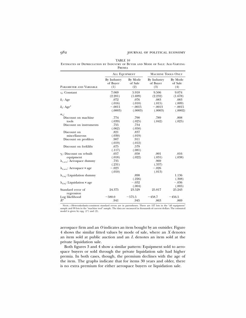
Table 10 shows the estimates of the more general model. Columns 1and 2 show the estimates for the sample of all equipment, and columns3 and 4 show the estimates for machine tools only. We find similar resultsacross all columns. The premia for both aerospace buyers and the privateliquidation sale appear to be a significant negative function of age. Atage equal to zero, the aerospace premium is estimated to be between74 percent and 100 percent, depending on the sample. At age equal tozero, the liquidation sale premium is estimated to be between 90 percentand 110 percent.

Figures 3 and 4 illustrate the temporal patterns implied by the esti-mates by showing the fitted values of q, which is the ratio of the predictedsales price to the reflated original cost. Using the estimates from col-umns 1 and 2 of table 10, we calculate the fitted values for a machinetool with the median reflated original cost and no rebuilds. Each agefor which we have at least one observation is represented by a point.In figure 3, an A indicates the fitted value for an item bought by an


TABLE 10Estimates of Depreciation by Industry of Buyer and Mode of Sale: Age-Varying

Premia


All Equipment Machine Tools Only

By Industryof Buyer

(1)

By Modeof Sale

(2)

By Industryof Buyer

(3)

By Modeof Sale

(4)

c0: Constant 7.069(2.201)

5.918(1.699)

9.506(2.232)

9.074(1.678)

d1: Age .072(.016)

.076(.010)

.083(.015)

.083(.009)

d2: Age2 �.0011(.0003)

�.0015(.0003)

�.0013(.0003)

�.0015(.0002)

am:Discount on machine

tools.774

(.039).790

(.025).789

(.042).808

(.025)Discount on instruments .755

(.062).734

(.050)Discount on

miscellaneous.821

(.030).837

(.019)Discount on profilers .907

(.019).911

(.012)Discount on forklifts .675

(.117).579

(.081)gr: Discount on rebuilt

equipment.057

(.018).058

(.022).001

(.031).016

(.038)l1,aero: Aerospace dummy .735

(.231).969

(.337)l2,aero: Aerospace#age �.023

(.010)�.026(.013)

l1,liq: Liquidation dummy .898(.226)

1.136(.308)

l2,liq: Liquidation#age �.032(.004)

�.036(.005)

Standard error ofregression

24.375 23.529 25.817 25.243

Log likelihood �580.0 �575.5 �458.7 �456.52R̄ .941 .945 .863 .869

Note.—Heteroskedastic-consistent standard errors are in parentheses. There are 127 lots in the “all equipment”sample and 99 lots in the “machine tool” sample. The data are measured in thousands of current dollars. The estimatedmodel is given by eqq. (1′′) and (2).

aerospace firm and an O indicates an item bought by an outsider. Figure4 shows the similar fitted values by mode of sale, where an X denotesan item sold at public auction and an L denotes an item sold at theprivate liquidation sale.

Both figures 3 and 4 show a similar pattern: Equipment sold to aero-space buyers or sold through the private liquidation sale had higherpremia. In both cases, though, the premium declines with the age ofthe item. The graphs indicate that for items 30 years and older, thereis no extra premium for either aerospace buyers or liquidation sale.


Fig. 3.—Fitted ratio of sales price to replacement cost by industry of buyer. Estimatesare based on col. 1 of table 10. An A denotes a lot sold to a buyer from the aerospaceindustry; an O denotes a lot sold to a buyer from a nonaerospace industry.

D. Limitations of the Estimates

The results of this section present evidence of a sizable wedge betweenthe replacement cost of capital and the value that a firm obtains whenit sells it. As the next section documents, these estimates need to beaugmented by the time cost of reallocation. This subsection briefly con-siders other reasons why our estimates might not be representative ormight not tell the whole story.

First, the value of the seller and the buyer of the equipment neednot be equal. The prices we analyze are what the seller received. Thebuyer typically pays an additional premium to the auction company(usually 10 percent). The buyer is also responsible for the cost of trans-portation and reinstallation. Additionally, standard auction theory sug-gests that the price paid at auction, on average, is equal to the second-highest valuation. The distance between the first- and second-highestvaluation depends on the distribution of valuations of the buyers. Sincewe were told that there were usually a good number of bidders on manyitems, we are led to believe that this wedge is not too large. In the caseof the private liquidation sales, the markets are thinner. Our resultsshow that the selling firm is able to extract more value in the private


Fig. 4.—Fitted ratio of sales price to replacement cost by mode of sale. Estimates arebased on col. 2 of table 10. An L denotes a lot sold in the private liquidation sale; an Xdenotes a lot sold in the public auction.

sale than in the auction. Our interpretation of this finding is that thecostly mechanism of the private liquidation sale facilitates achieving abetter match between buyer and seller. We do not know, however, howmany actual and potential customers there were in the private sales.Hence, though our results suggest that the private sale improved thematch between buyer and seller, we cannot assess quantitatively theefficiency of the market.

Second, the high discounts we find for the sale of capital could arisefrom adverse selection or low quality of the equipment. Yet, as men-tioned earlier, the equipment sold is not subject to the usual lemonsproblems because the plants we study were among the last closed bytheir respective firms and all their equipment was sold.16 Indeed, basingthe sample for the regressions on equipment that sold for more than$10,000 might bias our estimates upward. It is also unlikely that thelarge discounts were due to poor-quality equipment. Our industrysources report that the equipment in the aerospace industry is typically

16 Bond (1982) finds no evidence of lemons problems even in the market for usedtrucks. He compares maintenance costs of trucks bought used to those of trucks that havenot been traded and finds no significant difference.


well maintained. Finally, it is unlikely that the high discounts are dueto technological obsolescence. Our industry sources also told us thatthere has not been much technological advance in the type of machinetools used in aerospace manufacturing. The main advance is the use ofcomputer numerical control, which can be added to existing machines.In fact, many of the rebuilds in our sample consist of the addition ofcomputer numerical control. Thus we do not believe that lemons prob-lems, equipment quality, or technological obsolescence accounts for thehigh discounts we estimate.

Third, our estimates apply to the aerospace industry. To what extentare they applicable to other industries and to the economy overall? Theaerospace industry was in the midst of a dramatic downsizing. Hence,demand for aerospace-specific equipment was depressed relative to de-mand for equipment in general. Therefore, our estimates of the insiderpremia l are lower bounds on the value of specificity. Apart from theseaggregate demand conditions, how representative is aerospace in termsof the ex post flexibility of its capital? One of the auction experts toldus that in ratings of the ability to sell capital to other sectors, where 0implies no resale ability and 10 indicates great resale ability, the aero-space industry ranks a 10 compared to the steel industry at a 2. Thusone might expect other industries to suffer much larger losses duringa downturn.

It is enlightening to compare our results, which apply to a dramaticindustry downsizing and in which capital is only moderately fungible,to those for the resale of highly fungible capital in a growing industry.As mentioned above, Pulvino (1998, 1999) has analyzed the sale of usedaircraft by airlines. His data cover a period of industry expansion(1978–91) in which firms sold aircraft for idiosyncratic reasons ratherthan because of industrywide downsizing. At our request, he kindlyestimated a model similar to ours using his data on 391 aircraft sales.For the equation he estimated d to be .0280ageS p (1 � a)[(1 � d) I ],i i

(with a standard error of .0048) and a to be .0315 (with a standarderror of .030). The was .9317. Thus, in contrast to our results, the2R̄estimates from sales in the airline industry imply a Brainard-Tobin’s qof unity since a is not significantly different from zero. Of course, aircraftare among the easiest capital to reallocate within industry. Yet, were anairplane ever sold for some use other than air transport (an updateddiner?), the industry premium in such a regression would surely be verylarge.

E. Comparison with Labor

It is interesting to compare our findings for the cost of capital reallo-cation with similar results for labor. The loss in value appears to be


much higher than that found for workers in the aerospace industry. ARand report by Schoeni et al. (1996) studies the experiences of aero-space workers over this time period and thus is complementary to ourstudy of capital flows. Using state unemployment insurance records, theauthors gathered data on every worker who was employed in the aero-space industry in California in the first quarter of 1989. They foundthat one-third of the workers who remained with the same firm expe-rienced an 8 percent increase in real wages through the third quarterof 1994. The other two-thirds experienced some losses on average,though not out of line with the control group of displaced workers fromother durable goods industries. Nevertheless, even those workers whowere employed each quarter in California after separation from theirfirm experienced average wage losses of 4–5 percent relative to theirpreseparation earnings. Furthermore, one-quarter of this group sufferedreal wage losses of 15 percent or more. Thus these numbers are con-sistent with the literature showing that displaced workers generally ex-perience persistent income losses (e.g., Ruhm 1991).

It is difficult, however, to make a direct comparison to the estimatespresented in their study because they were unable to track individualswho left California. Thus the estimates they present pertain only tosubsamples. It is unlikely, though, that the unobserved group had suchlarge losses that they would raise the average loss to labor to anythingnear the estimates we found for capital. In summary, while substantial,these losses are far less than those suffered by capital.

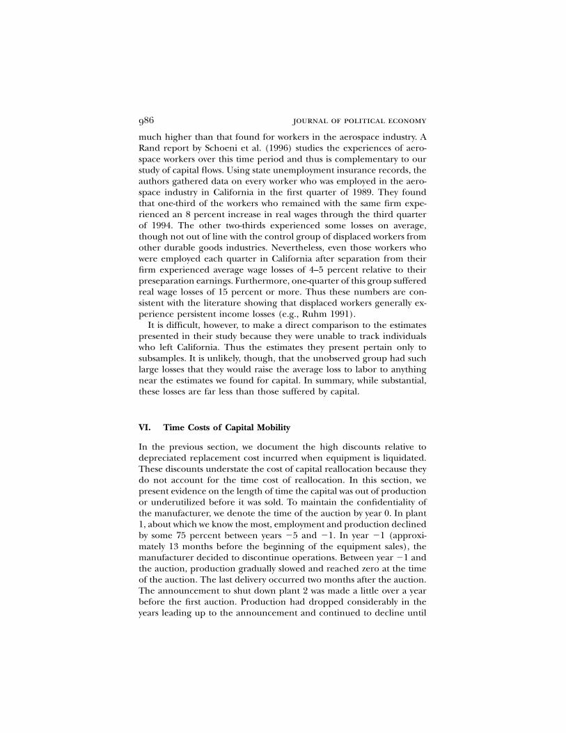
VI. Time Costs of Capital Mobility

In the previous section, we document the high discounts relative todepreciated replacement cost incurred when equipment is liquidated.These discounts understate the cost of capital reallocation because theydo not account for the time cost of reallocation. In this section, wepresent evidence on the length of time the capital was out of productionor underutilized before it was sold. To maintain the confidentiality ofthe manufacturer, we denote the time of the auction by year 0. In plant1, about which we know the most, employment and production declinedby some 75 percent between years �5 and �1. In year �1 (approxi-mately 13 months before the beginning of the equipment sales), themanufacturer decided to discontinue operations. Between year �1 andthe auction, production gradually slowed and reached zero at the timeof the auction. The last delivery occurred two months after the auction.The announcement to shut down plant 2 was made a little over a yearbefore the first auction. Production had dropped considerably in theyears leading up to the announcement and continued to decline until


the last equipment was sold. We do not have good information on thepattern of production at plant 3.

Thus, in one sense the sale of capital was swift, for it coincided withthe point at which production fell to zero. Capital utilization rates,however, were low both in the few years leading up to the decision todiscontinue operations and during the year of winding down. Thus therewas a prolonged period of declining utilization before the capital waseventually sold.

One aspect that struck us was that in some respects the dismantlingof the enterprise resulted in the more efficient use of the capital byallowing it to be sold. In contrast, there was another time at whichproduction was low but no capital was sold. In an earlier period of slackdemand, one of the facilities operated at very low levels of productionfor almost an entire decade. Our estimates suggest that a decision todisinvest is reversible only at great cost. Hence, this long period of lowutilization may well have been optimal.

The final issue on timing is the lag between the purchase of the capitalby the buyers and the use of that capital in production. We do not haveinformation on this issue, but we can offer some speculation. It is likelythat many pieces of equipment were used in production within a fewmonths of purchase since they did not require much setup. The out-come of the equipment that was sold to dealers is more uncertain. Itwould be interesting to find out how many dealers were able to resellthe equipment quickly and how many dealers held the equipment ininventory for speculation purposes.

We draw two conclusions on timing from this analysis. First, any pro-longed decrease in production probably results in significant periodsof underutilization of capital. Second, because of the large discountsexperienced on the sale of capital, the option value of a piece of installedcapital is very high. Thus firms may rationally choose to hold on tocapital for long periods of time in case production might rise in thefuture. It is only at times at which firms decide to cease operations thatthey sell significant portions of their capital.

VII. Conclusion

Our case study of aerospace suggests that capital is very costly to real-locate. This finding has implications for several important issues.

A. Investment Is Very Costly to Reverse, Especially during a SectoralDownturn

Our results provide direct evidence on the losses incurred when a firmmust sell its capital during a large sectoral downturn. For the subset of


equipment for which we had information, the estimates imply an averagereturn on replacement cost of only 28 cents on the dollar. We estimatethe instantaneous rate of depreciation to be 62 percent on machinetools, instruments, and miscellaneous equipment; 41 percent on fork-lifts; and 83 percent on profilers (from table 6). This degree of irre-versibility can have a major effect on investment behavior, as shown bythe theoretical results of Abel and Eberly (1994) and Dixit and Pindyck(1994).

B. Capital Displays Significant Sectoral Specificity

According to the auction experts, we are studying a sector with relativelyunspecific types of capital. Yet our calculations of the distribution ofcapital across sectors showed that aerospace was more heavily repre-sented among the buyers than one would expect if the capital wereperfectly fungible. Furthermore, we estimate significant premia for cap-ital that sold to industry insiders. For newer machine tools, the premiumwas 100 percent if it sold to another aerospace firm (table 10).

These results suggest an enormous degree of sectoral specificity. Dur-ing the time of our study, the marginal revenue product of capital inaerospace relative to other sectors plummeted. Yet, the value of muchof the equipment to aerospace was still significantly higher than tooutsiders. This fact implies a huge gap in the quality of the match ofthe capital characteristics to insiders versus outsiders. Owing to the lowstate of demand for aerospace, our estimates are a lower bound on thevalue of specificity.

As discussed earlier in the paper, the auctioneers and factory man-agers provided several reasons why some equipment would have highervalue to aerospace than to outsiders. First, the manufacture of aerospacegoods involves much larger pieces of metal than the manufacture ofmost other goods. Thus the machine tools for aerospace are muchbigger and must have higher horsepower than the average machinetool. Second, aerospace manufacturing requires much more precision,but lower volume, than many other types of manufacturing, such asautomobile production. Thus the high precision but low-volume abilitiesof the aerospace machine tools have less value to most companies out-side the aerospace industry.

C. Firms Engage in Costly Search and Matching to Overcome SectoralSpecificity and Market Thinness

Equipment in the private liquidation sale sold at a substantial premiumover equipment at the public auction. We believe that this premiumarises from the better matching of the specific characteristics of the


equipment sold to the needs of the buyer. The relatively thin marketfor specialized used equipment makes it profitable for both the buyerand seller to expend the time and resources entailed in a private saleto achieve a better match.

In summary, we suggest that the combination of sectoral specificityand thinness of markets impedes the efficiency of matching capital tonew owners. Thus reallocated capital is often placed in a lower-valueuse. If one could costlessly break down a wind tunnel into its constituentelements and costlessly reformulate it into another piece of equipment,it would have a much higher economic value than the immutable windtunnel that sold outside the aerospace sector.

Appendix

In order to determine how best to treat equipment that was rebuilt, we estimatethe following generalized version of the model in equations (1) and (2) in thetext:

S p c � (1 � a � g) 7 K � e (A1)i 0 m r i i

and2K p b 7 I 7exp {�[(d � d ) 7 age � d 7 age ]}. (A2)�i r iv 1 r iv 2 iv

v

This specification includes three parameters related to rebuilds: a different over-all return on the equipment (parameter gr in eq. [A1]), a different return onsubsequent investment for rebuilds (br in eq. [A2]), and a different depreciationrate on subsequent investments for rebuilds (dr in eq. [A2]). There are notenough data to estimate both br and dr at the same time, so we explore modelswith only one unconstrained at a time. The parameters gr and dr are zero forlots without rebuilds and possibly nonzero for lots with rebuilds. The parameterbr is one for lots without rebuilds; for lots with rebuilds, we consider specificationsin which it is nonzero, constrained to be zero, and constrained to be one.

Table A1 shows the results of various specifications. Column 1 allows a differentdiscount on initial investment in equipment that was subsequently rebuilt (gr)as well as a different contribution to value for rebuilds (br). The results suggestthat since gr is estimated to be significantly positive, rebuilt equipment actuallyreceives a discount in the market. The estimate of br is not significantly differentfrom zero, suggesting no return in the market to any additional investments forrebuilds. Column 2 explores an alternative specification by constraining br tobe unity and allowing the age-related depreciation rate on rebuilds to differ bydr. The very high depreciation rate dr has a similar implication to the high, age-invariant discount br: the market places little value on subsequent investmentsfor rebuilding equipment. This specification does not fit the data quite as wellas the previous one, though, as evidenced by the standard error of the regressionor the log likelihood function.

Column 3 gives our preferred specification, in which rebuilds have a discount(gr) and there is no return to subsequent investments ( ). A likelihoodb p 0r

ratio test does not reject this specification relative to the specification in column1. Moreover, the estimates of the other parameters of the model do not changenoticeably as a result of the constraints.

TABLE A1Estimates of Depreciation Rates and the Value of Rebuilds


br Unconstrained,dr p 0

(1)

br p 1,dr Unconstrained

(2)

br p 0,dr p 0

(3)

c0: Constant 1.038(2.428)

1.192(2.433)

1.764(2.404)

d1: Age .090(.013)

.089(.014)

.090(.014)

d2: Age2 �.0012(.0003)

�.0012(.0003)

�.0013(.0003)

am:Discount on machine tools .627

(.048).630

(.049).629

(.048)Discount on instruments .619

(.072).624

(.072).631

(.072)Discount on miscellaneous .686

(.021).688

(.022).688

(.022)Discount on profilers .834

(.024).836

(.024).836

(.024)Discount on forklifts .439

(.115).441

(.117).419

(.126)gr: Discount on rebuilt equipment .119

(.016).116

(.017).110

(.017)br: Return on subsequent

investment.243

(.148)1 0

dr: Age of subsequent investment 0 .512(.251)

0

Standard error of regression 26.341 26.490 26.432Log likelihood �590.4 �591.1 �591.4

2R̄ .931 .930 .931

Note.—Heteroskedastic-consistent standard errors are in parentheses. The sample consists of the 127 pieces ofequipment from plant 1. The data are measured in thousands of current dollars. The estimated model is given in eqq.(A1) and (A2).

TABLE A2Estimates of Depreciation: Structures Included

Parameter and Variable Baseline

c0: Constant 1.484 (2.593)d1: Age .071 (.021)d2: Age2 �.0008 (.0004)am:

Discount on machine tools .674 (.063)Discount on instruments .674 (.077)Discount on miscellaneous .713 (.029)Discount on profilers .864 (.030)Discount on forklifts .484 (.126)Discount on structures .959 (.019)

gr: Discount on rebuilt equipment .107 (.017)Standard error of regression 32.461Log likelihood �626.8

2R̄ .902

Note.—Heteroskedastic-consistent standard errors are in parentheses. The sample consists of 129 lots from the firstsale. The data are measured in thousands of current dollars. The estimated model is given by eqq. (1) and (2).


Table A2 shows estimates including observations on structures. These twoobservations are quite idiosyncratic, so we exclude them throughout the otherestimates in the paper.

References

Abel, Andrew B., and Eberly, Janice C. “A Unified Model of Investment underUncertainty.” A.E.R. 84 (December 1994): 1369–84.

———. “Investment and q with Fixed Costs: An Empirical Analysis.” Manuscript.Philadelphia: Univ. Pennsylvania, Wharton School, 1996.

Beidleman, Carl R. “Economic Depreciation in a Capital Goods Industry.” Nat.Tax J. 29 (December 1976): 379–90.

Bond, Eric W. “A Direct Test of the ‘Lemons’ Model: The Market for UsedPickup Trucks.” A.E.R. 72 (September 1982): 836–40.

———. “Trade in Used Equipment with Heterogeneous Firms.” J.P.E. 91 (August1983): 688–705.

Caballero, Ricardo J., and Engel, Eduardo M. R. A. “Explaining InvestmentDynamics in U.S. Manufacturing: A Generalized (S, s) Approach.” Econometrica67 (July 1999): 783–826.

Caballero, Ricardo J.; Engel, Eduardo M. R. A.; and Haltiwanger, John C. “Plant-Level Adjustment and Aggregate Investment Dynamics.” Brookings Papers Econ.Activity, no. 2 (1995), pp. 1–39.

Cockburn, Iain, and Frank, Murray. “Market Conditions and Retirement of Phys-ical Capital: Evidence from Oil Tankers.” Working Paper no. 4194. Cambridge,Mass.: NBER, October 1992.

Dixit, Avinash K., and Pindyck, Robert S. Investment under Uncertainty. Princeton,N.J.: Princeton Univ. Press, 1994.

Fraumeni, Barbara M. “The Measurement of Depreciation in the U.S. NationalIncome and Product Accounts.” Survey Current Bus. 77 (July 1997): 7–23.

Fuss, Melvyn A., and McFadden, Daniel L. “Flexibility versus Efficiency in ExAnte Plant Design.” In Production Economics: A Dual Approach to Theory andApplications, vol. 1, The Theory of Production, edited by Melvyn A. Fuss and DanielL. McFadden. Amsterdam: North-Holland, 1978.

Gordon, Robert J. The Measurement of Durable Goods Prices. Chicago: Univ. ChicagoPress (for NBER), 1990.

Hall, Robert E. “The Measurement of Quality Change from Vintage Price Data.”In Price Indexes and Quality Change: Studies in New Methods of Measurement, editedby Zvi Griliches. Cambridge, Mass.: Harvard Univ. Press, 1971.

Hulten, Charles R.; Robertson, James; and Wykoff, Frank C. “Energy, Obsoles-cence and the Productivity Slowdown.” In Technology and Capital Formation,edited by Dale W. Jorgenson and Ralph Landau. Cambridge, Mass.: MIT Press,1989.

Hulten, Charles R., and Wykoff, Frank C. “The Estimation of Economic Depre-ciation Using Vintage Asset Prices: An Application of the Box-Cox PowerTransformation.” J. Econometrics 15 (April 1981): 367–96.

———. “Issues in the Measurement of Economic Depreciation: IntroductoryRemarks.” Econ. Inquiry 34 (January 1996): 10–23.

Jorgenson, Dale W. “Empirical Studies of Depreciation.” Econ. Inquiry 34 (Jan-uary 1996): 24–42.

Oliner, Stephen D. “New Evidence on the Retirement and Depreciation of Ma-chine Tools.” Econ. Inquiry 34 (January 1996): 57–77.


Pulvino, Todd C. “Do Asset Fire Sales Exist? An Empirical Investigation of Com-mercial Aircraft Transactions.” J. Finance 53 (June 1998): 939–78.

———. “Effects of Bankruptcy Court Protection on Asset Sales.” Manuscript.Evanston, Ill.: Northwestern Univ., Kellogg Grad. School Management, 1999.

Ramey, Valerie A., and Shapiro, Matthew D. “Costly Capital Reallocation andthe Effects of Government Spending.” Carnegie-Rochester Conf. Ser. Public Policy48 (June 1998): 145–94. (a)

———. “Displaced Capital.” Working Paper no. 6775. Cambridge, Mass.: NBER,October 1998. (b)

Ruhm, Christopher J. “Are Workers Permanently Scarred by Job Displacements?”A.E.R. 81 (March 1991): 319–24.

Schoeni, Robert; Dardia, Michael; McCarthy, Kevin; and Vernez, Georges. “Lifeafter Cutbacks: Tracking California’s Aerospace Workers.” Report. Santa Mon-ica, Calif.: Rand Corp., Nat. Defense Res. Inst., 1996.

Stigler, George J. “Production and Distribution in the Short Run.” J.P.E. 47(June 1939): 305–27.

Veracierto, Marcelo. “Plant-Level Irreversible Investment and Equilibrium Busi-ness Cycles.” Working Paper no. WP-98-1. Chicago: Fed. Reserve Bank, 1997.

Wykoff, Frank C. “Capital Depreciation in the Postwar Period: Automobiles.”Rev. Econ. and Statis. 52 (May 1970): 168–72.

Displaced Capital: A Study of Aerospace Plant Closings

Documents

Transcript of Displaced Capital: A Study of Aerospace Plant Closings