DISPERSION MODELLING OF JET PROPELLANT 8 SPILL IN THE AEROSPACE INDUSTRY

A THESIS SUBMITTED TO THE GRADUATE SCHOOL OF NATURAL AND APPLIED SCIENCES

OF MIDDLE EAST TECHNICAL UNIVERSITY

BY

OLGUN ÇELİK

IN PARTIAL FULFILLMENT OF THE REQUIREMENTS FOR

THE DEGREE OF MASTER OF SCIENCE IN

OCCUPATIONAL HEALTH AND SAFETY

JANUARY 2020

Approval of the thesis:

DISPERSION MODELLING OF JET PROPELLANT 8 SPILL IN THE AEROSPACE INDUSTRY

submitted by OLGUN ÇELİK in partial fulfillment of the requirements for the degree of Master of Science in Occupational Health and Safety Department, Middle East Technical University by, Prof. Dr. Halil Kalıpçılar Dean, Graduate School of Natural and Applied Sciences

Prof. Dr. Mahmut Parlaktuna Head of Department, Occupational Health and Safety

Assoc. Prof. Dr. Çağlar Sınayuç Supervisor, Occupational Health and Safety, METU

Examining Committee Members: Prof. Dr. Yavuz Yaman Aerospace Engineering, METU

Assoc. Prof. Dr. Çağlar Sınayuç Petroleum and Natural Gas Engineering, METU

Prof. Dr. Mahmut Parlaktuna Petroleum and Natural Gas Engineering, METU

Prof. Dr. Ülkü Mehmetoğlu Chemical Engineering, Ankara University

Assist. Prof. Dr. İsmail Durgut Petroleum and Natural Gas Engineering, METU

Date: 29.01.2020

iv

I hereby declare that all information in this document has been obtained and

presented in accordance with academic rules and ethical conduct. I also declare

that, as required by these rules and conduct, I have fully cited and referenced all

material and results that are not original to this work.

Name, Surname:

Signature:

Olgun Çelik

v

ABSTRACT

DISPERSION MODELLING OF JET PROPELLANT 8 SPILL IN THE

AEROSPACE INDUSTRY

Çelik, Olgun

Master of Science, Occupational Health and Safety

Supervisor: Assoc. Prof. Dr. Çağlar Sınayuç

December 2019, 143 pages

The purpose of this study is to identify hazards, evaluate risks and suggest safety

measures in order to prevent fire and explosions due to the uncontrolled charging and

the ignition of jet propellant 8, shortly JP-8, at the fueling stations in the aerospace

industry. There are many different surveys on the ignition and the explosion of the

fuels in the literature. However, not enough researches have been made in order to

model the dispersion of the JP-8 spill in aviation. JP-8 is a petroleum product which

has wide usage in aviation as a jet engine propellant. JP-8 is a flammable hydrocarbon

mixture and its vapors can be ignited very quickly. JP-8 vapors can start a fire and

explode in open air or in the confined spaces in case of exposure to flame, spark, heat,

static electricity discharge and different types of ignition sources. A case scenario of

JP-8 spill during the fueling operations in the aviation sector is investigated to model

evaporation of JP-8 spill and dispersion of its vapors. Different evaporation and

dispersion models are discussed and compared for deciding the most suitable model

for the JP-8 spill. According to the assessment results, the area affected by the JP-8

spill and evacuation zones are defined. This research provides the required

information to design safe fueling stations and to increase the safety during fueling

operations for the aerospace industry.

vi

Keywords: Dispersion modelling, Evaporation modelling, Oil spill, Aerospace

vii

ÖZ

HAVACILIK SANAYİNDE JET YAKITI 8 DÖKÜNTÜSÜNÜN DAĞILIM

MODELLEMESİ

Çelik, Olgun

Yüksek Lisans, İş Sağlığı ve Güvenliği

Tez Danışmanı: Doç. Dr. Çağlar Sınayuç

Aralık 2019, 143 sayfa

Bu çalışmanın amacı havacılık sanayindeki yakıt istasyonlarında jet yakıtı 8’in, kısaca

JP-8, kontrol edilemeyen tutuşma ve ateşleme yüzünden patlamasını önlemek için

tehlikeleri belirlemek, riskleri değerlendirmek ve güvenlik önlemleri önermektir.

Literatürde yakıtların parlaması ve patlaması ile ilgili birçok farklı araştırma

mevcuttur. Fakat havacılıkta sektöründe JP-8 döküntüsünün havada dağılımını

değerlendiren yeterli miktarda araştırma henüz yapılmamıştır. JP-8 yanıcı bir

hidrokarbon karışımıdır ve buharı çok çabuk alevlenebilir. JP-8 buharları açık veya

kapalı ortamda alev, kıvılcım, ısı, statik elektrik ve diğer ateşleme kaynaklarına maruz

kalması durumunda patlayabilir. Havacılık sektöründeki yakıt işlemleri esnasında JP-

8 dökülmesi durum senaryosuna göre buharlaşma ve havada dağılım modellemesi

yapılmıştır. JP-8 döküntüsüne en uygun buharlaşma ve havada dağılım modelini

belirlemek için farklı buharlaşma ve havada dağılım modelleri araştırılmış ve

karşılaştırılmıştır. Araştırma sonuçlarına göre, JP-8 döküntüsünden etkilenen alanlar

ve tahliye bölgeleri belirlenmiştir. Bu araştırma, havacılık sanayinde güvenli yakıt

istasyonlarının tasarımı ve güvenliği artıracak yakıt işlemi kurallarının belirlenmesi

için gerekli bilgiyi sağlamaktadır.

viii

Anahtar Kelimeler: Dağılım modellemesi, Buharlaşma modellemesi, Petrol

döküntüsü, Havacılık

ix

To my beloved family...

x

ACKNOWLEDGMENTS

First of all, I would like to express my deepest appreciation to Assoc.Prof. Çağlar

Sınayuç. It was a great chance for me to work with him. His positive attitude,

encouragement and involvement kept me working harder. Without his supervision and

guidance, the whole thesis process would become much more challenging for me.

Besides my advisor, I would like to thank to all my Professors in the program for

sharing their wisdom and knowledge.

I would also like to thank all of my friends and colleagues for their contribution and

for sharing their experience throughout the thesis process.

Above all, I would like to express my gratefulness to my family for showing their

infinite love and endless support no matter what. I feel very lucky to have my mom,

Nazlı Çelik who feeds me with all her delicious and nutritious foods giving me the

energy that I need during my thesis marathon. I want to thank my dad, Ali Çelik who

advise me to have the patience that I require when I struggled. I want to show my

gratefulness to my sister, Duygu Gleissner for giving me motivation and being my

mentor every time I need. I love you all so much!

xi

TABLE OF CONTENTS

ABSTRACT ................................................................................................................. v

ÖZ ........................................................................................................................... vii

ACKNOWLEDGEMENTS ......................................................................................... x

TABLE OF CONTENTS ........................................................................................... xi

LIST OF TABLES ..................................................................................................... xv

LIST OF FIGURES ................................................................................................ xvii

LIST OF ABBREVIATIONS .................................................................................... xx

NOMENCLATURE ................................................................................................. xxi

CHAPTERS

1. INTRODUCTION ................................................................................................ 1

2. LITERATURE SURVEY ..................................................................................... 5

2.1. Fire and Explosions ........................................................................................... 5

2.1.1. The Fire Triangle ........................................................................................ 5

2.1.2. Distinction between Fires and Explosions .................................................. 7

2.1.3. Definitions .................................................................................................. 7

2.1.4. Explosions ................................................................................................. 10

2.1.4.1. Detonation and Deflagration .............................................................. 11

2.1.4.2. Blast Damage Resulting from Overpressure ...................................... 14

2.1.4.3. Vapor Cloud Explosions .................................................................... 15

2.2. Source of Ignition ............................................................................................ 16

2.2.1. Mechanical Ignition .................................................................................. 18

2.2.2. Electrical Ignition ..................................................................................... 18

xii

2.2.3. Open Flame .............................................................................................. 19

2.2.4. Hot Surfaces ............................................................................................. 21

2.2.5. Static Electricity ....................................................................................... 21

2.3. JP-8 and Kerosene ........................................................................................... 24

2.4. Fuel Servicing of Aircraft ............................................................................... 29

2.4.1. Electrostatic Hazards in Fuel Servicing and Static Grounding and Bonding

............................................................................................................................ 29

2.4.2. Fueling Procedures ................................................................................... 30

2.4.3. Fire Protection .......................................................................................... 32

2.5. Modeling JP-8 Evaporation ............................................................................ 34

2.5.1. Historical Development of Oil Evaporation Modeling ............................ 35

2.5.2. Development of Diffusion-Regulated Models ......................................... 46

2.5.3. Application and Comparison of Evaporation Models in Oil Spillages .... 52

2.6. Dispersion of Air Pollutants ............................................................................ 61

2.6.1. Weather .................................................................................................... 61

2.6.2. Turbulence ................................................................................................ 62

2.6.3. Topography .............................................................................................. 64

2.6.4. Dispersion Models .................................................................................... 65

2.6.5. Box Model ................................................................................................ 67

2.6.6. Gaussian Model ........................................................................................ 68

2.6.7. Dispersion Parameters .............................................................................. 73

2.6.8. Lagrangian Model .................................................................................... 78

2.6.9. Eulerian Model ......................................................................................... 80

2.6.10. Dense Gas Model ................................................................................... 81

xiii

3. STATEMENT OF PROBLEM ........................................................................... 83

4. METHODOLOGY ............................................................................................. 85

4.1. Introduction ..................................................................................................... 85

4.2. Fueling Operation Area and Fuel Spill Accident Conditions .......................... 86

4.3. Evaporation Model of JP-8 .............................................................................. 87

4.4. Dispersion Model of JP-8 ................................................................................ 91

5. RESULTS AND DISCUSSIONS ....................................................................... 95

5.1. Results and Discussions for Evaporation Modelling ...................................... 95

5.2. Vapor Pressure Calculation ............................................................................. 95

5.2.1. Blokker’s Model ....................................................................................... 96

5.2.2. Fingas (2013) Model ................................................................................. 96

5.2.3. Jenkins (2008) Model ............................................................................... 97

5.2.4. Tkalin’s Model .......................................................................................... 98

5.3. Mass Transfer Constant Calculation ............................................................... 99

5.3.1. Mackay & Matsugu Formulation for Mass Transfer Constant ................. 99

5.3.2. Hamoda Formulation for Mass Transfer Constant ................................. 100

5.3.3. Tkalin’s Formulation for Mass Transfer Constant ................................. 101

5.4. Evaporation Calculation ................................................................................ 102

5.4.1. Stiver and Mackay Evaporation Model .................................................. 102

5.4.2. Tkalin’s Evaporation Model ................................................................... 103

5.4.3. Brighton’s Evaporation Model ............................................................... 103

5.4.4. Evaporation Modelling with Empirical Equation ................................... 104

5.4.5. Mackay and Wesenbeeck Evaporation Model........................................ 106

5.5. Results and Discussions for Dispersion Modelling ....................................... 107

xiv

5.5.1. Determination of σy and σz According to Pasquill’s Atmospheric Stability

Classes Method ................................................................................................. 108

5.5.2. Calculation of σy and σz According to Briggs Formulation ................... 110

5.5.3. Application of Gaussian Dispersion Model ........................................... 113

5.6. The Effect of Amount of Spill and Spillage Area ......................................... 115

5.7. The Effect of Temperature ............................................................................ 115

5.8. The Effect of Wind Speed in The Open Air ................................................. 119

5.9. The Effect of Atmospheric Stability Class ................................................... 122

5.10. The Effect of Land Characteristic ............................................................... 122

5.11. Model Accuracy and Limitations ................................................................ 122

6. CONCLUSION ................................................................................................ 125

7. RECOMMENDATION .................................................................................... 129

REFERENCES ........................................................................................................ 133

xv

LIST OF TABLES

TABLES

Table 2.1. Main Factors That Affect Explosion Process (Crowl & Louvar, 2011) ... 10

Table 2.2. Flash Points of Flammable Chemical Vapors ........................................... 20

Table 2.3. Effect of Wind Velocity in AITs Using Kerosene (API, 2003) ................ 21

Table 2.4. Petroleum Products (Speight & El-Gendy, 2018) ..................................... 25

Table 2.5. Assumed Average Formula of Petroleum Fuels (Totten et al., 2003) ...... 26

Table 2.6. Heat of Vaporization of Oil Products (Speight, 2017).............................. 26

Table 2.7. Properties of Hydrocarbon Products from Petroleum (Speight, 2011) ..... 27

Table 2.8. Chemical and Physical Requirement (U.S. Department of Defense, 2015)

.................................................................................................................................... 28

Table 2.9. Maximum Allowable Fueling Rates (USAF, 2013) ................................. 30

Table 2.10. Saturation Concentration of Water and Hydrocarbons (Fingas, 2013) ... 49

Table 2.11. Sample of Empirical Equations of Oil Evaporation (Fingas, 2013) ....... 52

Table 2.12. Evaporation Rate Coefficients of Several Substances at 25 °C According

to Equation 47 (Mackay and Wesenbeeck, 2014) ...................................................... 59

Table 2.13. Pasquill’s Atmospheric Stability Classes ................................................ 63

Table 2.14. Key to Stability Categories ..................................................................... 63

Table 2.15. Experimental Coefficients Determined by Briggs (1973) (De Visscher,

2014). ......................................................................................................................... 75

Table 4.1. The Values of the Physical and Environmental Factors ........................... 87

Table 5.1. Vapor Pressure of Kerosene According to Various Models ..................... 95

Table 5.2. Mass Transfer Constant of Kerosene According to Various Models ....... 99

Table 5.3. Evaporation Rate of JP-8 spill According to Various Models ................ 102

Table 5.4. Percentage Evaporated and Evaporation Rate at Various Time After Spill

.................................................................................................................................. 106

Table 5.5. Key to Stability Categories ..................................................................... 108

xvi

Table 5.6. 𝜎𝑦 and 𝜎𝑧 Values According to Pasquill’s Model. ................................ 110

Table 5.7. Experimental coefficients determined by Briggs ................................... 111

Table 5.8. 𝜎𝑦 and 𝜎𝑧 Values According to Briggs Formula ................................... 112

Table 5.9. Comparison of 𝜎𝑦 and 𝜎𝑧 Values According to Briggs Formula and

Pasquill’s Method .................................................................................................... 112

xvii

LIST OF FIGURES

FIGURES

Figure 2.1. Fire Triangle (Crowl & Louvar, 2011) ...................................................... 6

Figure 2.2. Relationships Between Various Flammability Properties (Crowl & Louvar,

2011). ........................................................................................................................... 9

Figure 2.3. Comparison of Physical Differences between Detonation and Deflagration

.................................................................................................................................... 13

Figure 2.4. Blast Pressure Change at a Certain Point versus Time (Crowl & Louvar,

2011). ......................................................................................................................... 15

Figure 2.5. Ignition Process of Flammable Vapors by Electrostatic Electricity

(Hattwig & Steen, 2004) ............................................................................................ 22

Figure 2.6. The Physical Parameters Affecting the Ignition Process of Flammable

Vapors by Electrostatic Electricity (Hattwig & Steen, 2004) .................................... 24

Figure 2.7. Fuel Servicing Safety Zone (FSSZ) ......................................................... 32

Figure 2.8. Evaporation Rates of Gasoline versus Various Wind Speed (Fingas 2013).

.................................................................................................................................... 46

Figure 2.9. Evaporation Rates of ASMB versus Various Wind Speed (Fingas 2013).

.................................................................................................................................... 47

Figure 2.10. Evaporation Rates of Water versus Various Wind Speed (Fingas 2013).

.................................................................................................................................... 47

Figure 2.11. Wind Velocity versus Evaporation Rates (Fingas, 2013) ...................... 48

Figure 2.12. Evaporation Rate Modelling of Diesel Oil with Air-layer-boundary

Equation (like equation (33)) versus Experimental Data Given in Table 11 (Fingas,

2013) .......................................................................................................................... 54

Figure 2.13. Evaporation Rate Modelling of Bunker C with Air-layer-boundary

Equation (like equation (33)) versus Experimental Data Given in Table 11 (Fingas,

2013) .......................................................................................................................... 55

xviii

Figure 2.14. Evaporation Rate Modelling of Pembina Crude Oil with Air-layer-

boundary Equation (like equation (33)) versus Real Data and Experimental Curve

(Fingas, 2013) ............................................................................................................ 56

Figure 2.15. Plot of Molar Evaporation Rate, E vs. Pressure, P ................................ 58

Figure 2.16. The Effect of a Building to the Flow of Wind ...................................... 64

Figure 2.17. Effect of Urban, Suburbs and Rural Areas on Wind Speed (Turner, 1994)

................................................................................................................................... 65

Figure 2.18. Box Model Diagram (Hanna et al., 1982) ............................................. 68

Figure 2.19. Gaussian Dispersion Model (Nesaratnam and Taherzadeh, 2014). ...... 70

Figure 2.20. Non-buoyant Gaussian Dispersion from a Ground Source (Pursuer et al.,

2016). ......................................................................................................................... 71

Figure 2.21. Reflected source due to ground reflection (Cooper and Alley, 2011) .. 71

Figure 2.22. Horizontal Dispersion Coefficient, σy , vs. Downwind Distance, x

(Godish, 2004). .......................................................................................................... 74

Figure 2.23. Vertical Dispersion Coefficient, σz , vs. Downwind Distance, x (Godish,

2004). ......................................................................................................................... 74

Figure 2.24. (a) Horizontal, σy , and (b) vertical, σz , Dispersion Coefficients

Formulated by Briggs (1973) (solid lines) and Martin (1973) (dotted lines) vs.

Downwind Distance, x in Rural Area (De Visscher, 2014) ...................................... 77

Figure 2.25. Movement of a Particle in the Random Walk Model (Vallero, 2014) .. 78

Figure 2.26. Lagrangian Model for a Vertical Column of Boxes (Zannetti,1990). ... 79

Figure 2.27. Scheme of Reference Frame for Eulerian (a) and Lagrangian (b)

dispersion Model (Zannetti,1990) ............................................................................. 80

Figure 5.1. Vapor pressure line of kerosene according to Blokker ........................... 96

Figure 5.2. Vapor pressure line of kerosene according to Fingas (2013) .................. 97

Figure 5.3. Vapor pressure line of kerosene according to Jenkins (2008) ................ 98

Figure 5.4. Vapor pressure line of kerosene according to Tkalin’s Evaporation Model

................................................................................................................................... 98

Figure 5.5. Mass Transfer Constant vs. Wind Speed According to Mackay&Matsugu

(1973) ....................................................................................................................... 100

xix

Figure 5.6. Mass Transfer Constant vs. Temperature According to Hamoda et al.

(1989) ....................................................................................................................... 101

Figure 5.7. Mass Transfer Constant vs. Wind Speed According to Tkalin’s

Evaporation Model ................................................................................................... 102

Figure 5.8. Percentage Evaporated vs. Time According to Empirical Equation ..... 105

Figure 5.9. Evaporation Rate vs. Time According to Empirical Equation .............. 105

Figure 5.10. Horizontal dispersion coefficient, σy , vs. Downwind distance, x (Godish,

2004). ....................................................................................................................... 109

Figure 5.11. Vertical dispersion coefficient, σz , vs. Downwind distance, x (Godish,

2004). ....................................................................................................................... 109

Figure 5.12. JP-8 Vapor Concentration vs. Downwind Distance ............................ 114

Figure 5.13. Vapor Concentration vs. Downwind Distance at 10 °C Temperature . 117

Figure 5.14. Vapor Concentration vs. Downwind Distance at 40 °C Temperature . 118

Figure 5.15. Vapor Concentration vs. Downwind Distance at 0.5 m/s Wind Speed

.................................................................................................................................. 120

Figure 5.16. Vapor Concentration vs. Downwind Distance at 6 m/s Wind Speed .. 121

xx

LIST OF ABBREVIATIONS

ABBREVIATIONS

AIT : Autoignition temperature

JP-8 : Jet propellant 8

LFL : Lower flammability limit

UFL : Upper flammable limit

VCE : Vapor cloud explosion

ISO : International Organization for Standardization

NFPA : National Fire Protection Agency

MIE : Minimum ignition energy

SPR : Single point refuel

FSSZ : Fuel servicing safety zone

ASMB : Alberta Sweet Mixed Blend

PBL : Planetary boundary layer

TLV : Threshold limit value

TWA : Time weighted average

LEL : Lower explosion limit

UEL : Upper explosion limit

DDT : Deflagration to detonation transition

xxi

NOMENCLATURE

Roman Symbols:

a Experimental constant in Briggs (1973) formula

A Area of oil layer

b Experimental coefficient in Briggs (1973) formula

c Experimental coefficient in Briggs (1973) formula

C Concentration

𝑐0 Equilibrium concentration of vapor at the top layer of

the oil

𝐶𝑠 Evaporating liquid concentration

d Experimental coefficient in Briggs (1973) formula

da Pool area

d1 Pool length

D Oil spill diameter

Di Diffusivity

e Experimental coefficient in Briggs (1973) formula

E Evaporation rate

𝐸𝑖 Evaporation rate of oil compound I or total evaporation

f Experimental coefficient in Briggs (1973) formula

Fv Volume of the evaporated compound

h Effective height

H Henry’s law constant

k Experimental rate

𝑘𝑚 Constant which involves all factors related to 𝐾

kv Von Karman coefficient

K Mass transfer constant

𝐾𝑚𝑎 Constant which includes all factors concerning oil

evaporation after the surface film formed

xxii

𝐾𝑚𝑏 Constant which includes all factors concerning oil

evaporation before the surface film formed

𝐾𝑒𝑣 Atmospheric stability coefficient

M Molecular weight

n Power law dimensionless parameter

N Carbon number of oil product

P Vapor pressure

𝑃𝑖 Vapor pressure of oil compound, i, on the boundary

𝑃𝑖∞ Vapor pressure of oil compound, i, at infinite altitude

Poi Vapor pressure of the oil compound i

Ps Vapor pressure at boiling point

𝑃𝑣 Saturated vapor pressure

R Universal gas constant

q Experimental constant in Yang and Wang (1977)

equation.

𝑄 Emission rate

S Saturation factor

Sn Sink term

Sc Schmidt number

T Time

T Temperature

Ts Boiling point temperature

Tu Relative intensity factor of turbulence

U Velocity of wind

𝑢∗ Friction velocity

v Molar volume of the liquid

V0 Volume of the spillage at the beginning

x Amount of specific oil product at time t

xo Amount of specific oil product at time t equals zero

xxiii

X Pool diameter

𝑧1 Height above the surface

𝑧0 Roughness length

%D Percentage distilled by weight

Greek Symbols:

𝛼 Meteorological coefficient

𝛼1 Coefficient which is the combination of wind speed

and all factor

𝛽 Meteorological coefficient

∆𝑣𝑎𝑝𝐻0 Heat of evaporation

∆ℎ Drop in thickness of layer

𝛾 Experimental constant in Yang and Wang (1977)

equation.

𝜎𝑦 Horizontal dispersion parameter

𝜎𝑧 Vertical dispersion parameter

𝜃 Evaporative exposure

Superscripts:

r Experimental value in Brighton model

1

CHAPTER 1

1. INTRODUCTION

The aviation sector is growing very rapidly for decades in Turkey. Accordingly, the

number of accidents in the aviation sector is increasing. Accidents resulting from

fueling operations are major concerns of safety in aviation. Many explosions and fire

accidents occur during the fueling process of aircrafts. One of the main causes of fires

and explosions is ignition of fuel vapors, mists and sprays due to uncontrolled ignition

source during the fueling operations. Additionally, fuel has a toxic effect on humans

who are exposed to its vapors by inhalation.

The fuel vapors can arise from various liquid fuel sources such as fuel storage tanks,

fuel tanks of aircraft or fuel spills on the flight line. In the case of a fuel spill, liquid

fuel evaporates continuously and fuel vapors are emitted from the spill to the air. Fuel

vapors disperse in the air and are carried away from the source by the effect of wind.

According to the emission rate of fuel vapors from the source, vapor concentration

can rise up to flammability range and toxic level. Thus, the consequences of fuel spill

are needed to be forecasted in order to identify possible risks and maintain safety in

fueling operations. In order to estimate the possible consequences of the JP-8 spill, the

dispersion mechanism of fuel vapors is needed to be understood.

Crowl & Louvar (2011) states that fuel, oxidizer and ignition source are the main

elements of fire. Fire is an exothermic oxidation reaction of ignited fuel. Fuel, oxidizer

and an ignition source should be present in the adequate amount to start a fire process.

If not, the burning of fuel does not occur. To prevent fire and explosion, ignition

sources should be kept under control and flammable atmospheric condition should be

eliminated.

2

Jet fuel is a petroleum product and has different types of usage in aircraft engines. JP-

8 is kerosene typed fuel which is used in aviation. According to the U.S. Department

of Defense (2015), JP-8 has wide usage because of its safely handling characteristics

and benefits in usage such as low icing point. Ghassemi et al. (2006) says that kerosene

and dodecane, C12H26, have very similar properties. Kerosene is more volatile than

diesel oil but not more volatile than gasoline (Speight & El-Gendy, 2018).

Dispersion modelling of the JP-8 spill requires determination of emission rate of fuel

vapors which is equal to the evaporation rate of the JP-8 spill. There are several

evaporation models for calculation of the evaporation rate of kerosene. Five main

approaches are used and compared in evaporation modelling. Most evaporation

models regard the evaporation rate as constant during the evaporation process.

However, approaches like the empirical equation model have a logarithmic rate of

evaporation. Thus, each model has advantages and drawbacks. The most important

point in modeling is to select the most suitable model regarding the simulated case

scenario.

Mass transfer constant is also required for evaporation rate calculation. Various

models are present for mass transfer constant determination. Mainly, mass transfer

constant formulas are empirical and obtained by laboratory experiments. Some of the

mass transfer constant formulas are complex and require several information about the

spill. On the contrary, some models are simple and easy to apply. Three widely used

model is applied for evaporation modeling and results are assessed.

Numerous dispersion models are available for approximation of chemical vapors

concentration emitted from pollutant sources. In order to decide the most suitable

dispersion model, emission rate, emission duration and type of source should be

known. In this thesis, five main dispersion models are discussed. Gaussian dispersion

model is used for determining vapor concentrations arising from JP-8 spill in

downwind distances. In the Gaussian dispersion model, it is assumed that the vapor

concentration of JP-8 has Gaussian distribution over the lateral and vertical axis.

3

Variation of concentration in axis is correspondent to atmospheric stability class and

downwind distance from the spill.

In this current work, the scenario of JP-8 spill from the fueling system to the flight

line due to misconduct in fueling operation is evaluated. According to the spill

accident scenario, JP-8 is stored next to fueling hangars and fueling operations of

aircraft are conducted in this area. Spillage of JP-8 evaporates immediately and the

JP-8 vapor will disperse into the air by the wind. Possible safety and health concerns

such as fire, explosion and exposure to chemical vapors are discussed. As an outcome

of this study, required safety measures to maintain safe fueling operations are advised.

5

CHAPTER 2

2. LITERATURE SURVEY

2.1. Fire and Explosions

Chemicals can cause important fire and explosion hazards. According to Crowl &

Louvar (2011), in United States, chemical and hydrocarbon plants were estimated to

have $300 million worth of property losses in addition to life losses and production

stoppage in 1997 as a result of fire and explosions.

Crowl & Louvar (2011) say that the prevention of fires and explosion can only be

provided by knowing fire and explosion characteristics of chemicals, by

understanding the process of fire and explosion and recognizing the ways of reducing

fire and explosion probability.

2.1.1. The Fire Triangle

According to Crowl & Louvar (2011), the important components of the fire process

are fuel, oxidizer and ignition source. Figure 2.1. provides an understanding of fire

process and its components.

6

Figure 2.1. Fire Triangle (Crowl & Louvar, 2011)

According to Crowl & Louvar (2011), fire can be described as a fast exothermic

oxidation reaction of ignited fuel. The fuel can be in many different forms such as

solid, liquid or vapor however vapors of liquid fuels are easier to be ignited. Before

the combustion process, liquids are volatized and solids are decomposed into the

gaseous phase, accordingly, the process of combustion is always conducted in the

vapor phase.

In order to fire process to occur, fuel, oxidizer and an ignition source should be

available in a sufficient amount. Therefore, burning will not take place in case of

absence or insufficiency of fuel or oxidizer and if ignition source does not have

sufficient energy to start the fire.

In the past decades, the main methodology for fire and explosion control was to

eliminate or reduce the source of ignition. However, it was realized that eliminating

or reducing sources of ignition is not adequate for fire and explosion prevention since

the required energy for ignition of flammable chemicals is very low and there are

various sources of ignition. Therefore, it was found to be more effective in fire and

7

explosion control to eliminate sources of ignition while avoiding flammable

atmospheric conditions to occur.

Many different types of fuels, oxidizers and ignition sources can be found in the

aviation industry. Fuels and oxidizers can be in the form of solid, liquid or gas.

Additionally, ignition sources can be found as sparks, flames static electricity and heat.

2.1.2. Distinction between Fires and Explosions

Crowl & Louvar (2011) states that the main difference between fire and explosion is

the energy output rate. In burning process, the energy output rate is slower than the

explosion energy release rate which is in degrees of microseconds. Fires can be

initiated by explosions and also explosions can be caused by fires.

2.1.3. Definitions

Fire or combustion can be defined as a chemical process in which a material reacts

with an oxidizing agent and outputs some energy.

Ignition can be initiated by interaction of ignition source with the required energy and

flammable gas in high temperatures which is sufficient for flammable gas to auto-

ignite (Crowl & Louvar, 2011).

Autoignition temperature (AIT) is the minimum required temperature for the ignition

of a combustible gas by its own heat in the absence of a glow or flame. An increase in

chain length of straight-chain hydrocarbons causes AIT to decrease (Nolan, 2014).

Flash point is the minimum temperature at which combustible vapors can be ignited

by an ignition source (Hattwig & Steen, 2004). One of the main characteristics to

specify fire and explosion hazard of liquids is the flash point temperature.

8

Fire point is the minimum temperature for a flammable gas to maintain burning after

ignition (Crowl & Louvar, 2011).

Lower Flammability Limit (LFL) is the lowest concentration of a flammable gas in

air below which ignition cannot take place (Moosemiller, 2014). Flammable limits

and explosive limits are the technical terms which can be used interchangeably (Nolan,

2014).

Explosion can be described as a sudden discharge of energy resulting in a blast (Baker

et al., 2010).

Blast is a temporary alteration in the density gas mixture, pressure and speed of air

flow at the surrounding of an explosion source (Baker et al., 2010).

Confined explosion occurs inside an enclosed volume such as tank, container or

structure. Confined explosion is the most destructive type of explosion causing injury

and demolition of buildings.

An unconfined explosion occurs in the open atmosphere. Unconfined explosions are

mostly caused by flammable chemical spillage. As a result of a spill, flammable vapors

disperse in the air and can form an explosive mixture with air until it is ignited by an

ignition source. Unconfined explosions are not common since explosive vapors are

diluted by wind below the LFL. On the other hand, unconfined explosion can also be

very damaging since a huge amount of flammable vapor is involved (Crowl & Louvar,

2011).

Deflagration is caused by an explosion where the propagation of the reaction front

occurs at a speed slower than the speed of sound in front of the pressure front (Vinnem,

2014).

Detonation is the dispersion of energy resulting from a very fast chemical reaction in

which reaction front moves outward from explosion source at higher than the speed

of sound (Woodward, 1998).

9

Shock wave is a sudden pressure wave causing strong wind. The combination of shock

wave and wind is known as blast wave. Shock wave has a very fast pressure rise which

is a mostly adiabatic process (Crowl & Louvar, 2011).

Overpressure is negative or positive pressure which is formed as a result of an

explosion (Nolan, 2014).

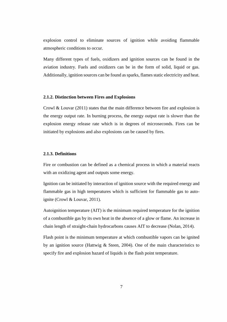
Figure 2.2. Relationships Between Various Flammability Properties (Crowl & Louvar, 2011).

In figure 2.2, it can be seen the graph of concentration of flammable vapor versus

temperature and the relationship of the above definitions. The exponential curvature

signifies the saturation vapor pressure curve of the liquid substance. As usual, upper

flammable limit (UFL) becomes higher and lower flammable limit (LFL) becomes

10

lower with an increase in temperature. In theory, the intersection point of LFL and the

saturation vapor pressure curve of the liquid represents flash point however sometimes

empirical data does not validate this idea. The lowest temperature of the autoignition

curve gives the autoignition temperature. The flash point and flammability limits are

not the main characteristics of a liquid and can only be identified by special laboratory

equipment.

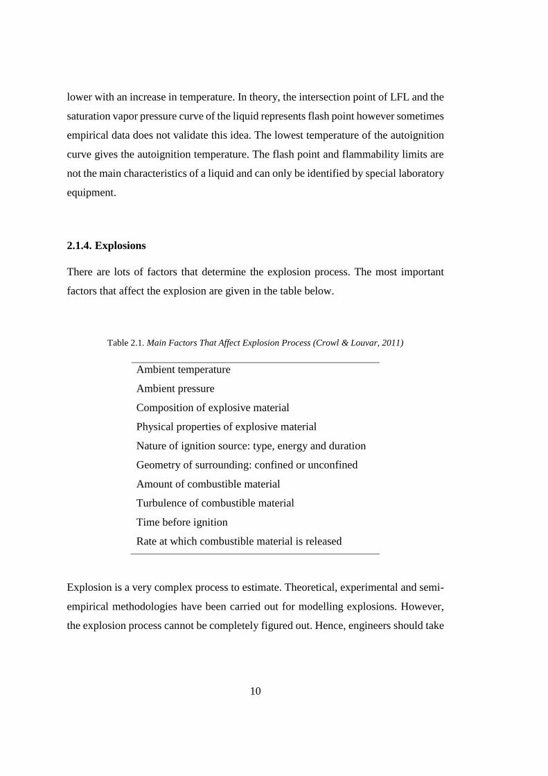
2.1.4. Explosions

There are lots of factors that determine the explosion process. The most important

factors that affect the explosion are given in the table below.

Table 2.1. Main Factors That Affect Explosion Process (Crowl & Louvar, 2011)

Ambient temperature

Ambient pressure

Composition of explosive material

Physical properties of explosive material

Nature of ignition source: type, energy and duration

Geometry of surrounding: confined or unconfined

Amount of combustible material

Turbulence of combustible material

Time before ignition

Rate at which combustible material is released

Explosion is a very complex process to estimate. Theoretical, experimental and semi-

empirical methodologies have been carried out for modelling explosions. However,

the explosion process cannot be completely figured out. Hence, engineers should take

11

into consideration all probable outcomes carefully in order to guarantee safety in

designing.

Explosions are caused by a very fast release of energy. The discharge of energy must

be very quick to provide energy to accumulate at the blast source. After that, the

energy is dispersed by pressure wave, projectiles, thermal radiation, and acoustic

energy. The disposed energy causes the explosion damage.

If a gas explosion occurs, immediately gas starts to disperse very fast to the

environment causing a pressure wave that pushes nearby gases backward from the site

of the explosion. The energy contained in the pressure wave causes surroundings to

be damaged. For chemical explosions, the main factor that causes damage is the

pressure wave. Therefore, the dynamics of the pressure wave should be understood to

predict explosion damage.

The pressure wave dispersing outward from the explosion is also known as the blast

wave since a strong wind occurs after the explosion. A shock wave or shock front is

caused in case of sudden pressure change. Very explosive chemicals can cause a shock

wave to occur. The maximum pressure reached after an explosion is known as the

peak overpressure.

2.1.4.1. Detonation and Deflagration

According to Crowl & Louvar (2011), the damage of the explosion is mainly

dependent on whether the explosion is a result of detonation or deflagration. The

distinction relies upon whether the reaction front disperses above or below the speed

of sound in the ambient atmosphere. The speed of sound is 344 m/s regarding ideal

gases at 20 °C and it only varies with temperature.

In detonation, the reaction front is transferred by a very high-pressure wave that

pressurizes the ambient air in front of the reaction front above its autoignition

temperature. This sudden pressure change causes a shock front to occur in front of the

12

reaction front. So, the front wave and the shock wave disperse at the speed of sound

into the surrounding atmosphere.

In deflagration, explosion energy disperses into ambient air by heat conduction and

molecular diffusion. Since these transfer processes are slower than the speed of sound,

the reaction front disperses slower than sonic speed.

In figure 2.3, the gas dynamics of detonation and deflagration in the open air are

compared. In detonation, the movement speed of the reaction front is greater than

sonic velocity. A shock front is present in front of the reaction front. For the shock

front to move at the speed of sound, the required energy is provided by the reaction

front. Both fronts move at the same velocity. In deflagration, movement speed of

reaction front is lower than sonic velocity while pressure front disperses at the speed

of sound and moves away from the reaction front. Therefore, it can be thought that the

deflagration reaction front produces a series of separate pressure fronts continuously.

Resulting pressure fronts added to each other and collected in the main pressure front.

The main pressure front grows continuously as additional energy is accumulated.

13

Figure 2.3. Comparison of Physical Differences between Detonation and Deflagration

(Crowl & Louvar, 2011)

Detonation and deflagration produce pressure fronts which are obviously different

from each other. In detonation, a shock front is formed with sudden pressure change

of about 10 atm for a duration of 1 millisecond. In deflagration, a shock front is not

formed and the pressure front lasts for many milliseconds and has lower pressure

characteristically 1 or 2 atm.

Reaction fronts and pressure fronts can differ because of the enclosing environment

of the explosion source. Altered behaviors of fronts can be observed if the explosion

occurs in a confined volume like a vessel or a pipeline.

14

According to Crowl & Louvar (2011), the transformation of a deflagration to

detonation can be observed in some cases. This transformation is known as

deflagration to detonation transition (DDT). DDT can occur in pipelines however, it

is not likely to occur in vessels and open air. In pipelines, deflagration energy provides

additional pressure to the main pressure wave causing pressure increase which can

result in detonation.

2.1.4.2. Blast Damage Resulting from Overpressure

After the explosion of a gas, whether detonation or deflagration, the reaction front is

occurred dispersing from explosion source and it is followed by a shock wave or

pressure wave. After the combustion reaction is complete, the reaction front

disappears but the pressure front carries on to its movement. A blast wave consists of

a pressure front and resulting wind. Most of the damage is caused by the blast wave.

Figure 2.4 provides an understanding of chance in blast pressure over time for a

characteristic shock wave at a certain point away from the explosion source. In figure

2.4, t0 represents time of explosion, t1 signifies the arrival time of blast pressure to

damaged location from explosion source. At t1, shock front causes maximum

overpressure to occur and followed by subsequent wind at a fixed location. The blast

pressure reduces rapidly to the ambient pressure at t2 but the wind continues to move

forward for a period of time. The time interval between t1 and t2 is known as shock

duration. The shock duration has the most destructive effect on surrounding structures

during an explosion thus, it is important to know its value to assess the damage. Since

the pressure continues to decrease below the ambient pressure, at t3, the maximum

underpressure is reached. For the time period between t2 and t4, the explosion wind

moves in the opposite direction towards the explosion source. There can be some

damage caused by underpressure, however, the damage is limited compared to

overpressure damage. From t3 to t4, the pressure increases and reaches ambient

pressure at t4. At t4, the explosion wind and destruction effect is over.

15

Figure 2.4. Blast Pressure Change at a Certain Point versus Time (Crowl & Louvar, 2011).

The blast damage can be determined by peak overpressure that is caused by the

pressure wave of the explosion. Generally, the blast damage depends on the pressure

increase rate and time period of the blast wave. Accurate estimation of blast damage

can be estimated by just using the peak overpressure (Crowl & Louvar, 2011).

2.1.4.3. Vapor Cloud Explosions

According to Crowl & Louvar (2011), vapor cloud explosions (VCEs) causes the most

damaging effect in chemical operations. VCEs has three occurrence steps:

1. Immediate discharge of huge amount of flammable vapor (such as vessel brust)

2. Dispersal of flammable vapors through the operation area

3. Ignition of flammable vapors

16

The occurrence rate of VCEs is increasing in process plants since the number of

flammable chemicals is also increasing and operations are conducted in harder

conditions. It is very hard to classify an event as a VCEs since there are lots of

parameters that are needed to describe an event. VCEs happen under uncontrolled

conditions and real incident data are not reliable for comparison.

The most important factors that affect VCE are amount of flammable vapor discharge,

concentration of flammable vapor in the air, ignition probability of flammable gas

vapor, dispersion distance of vapor cloud, duration before ignition of flammable gas,

possibility of explosion, presence of threshold amount of gas, effectiveness of

explosion and position of the ignition source.

Crowl & Louvar (2011) says that ignition possibility of flammable vapor cloud

increases if the volume of cloud increases, VCEs are much unlikely to happen

compared to vapor cloud fires, effectiveness of explosion is low (around 2% of the

combustion energy is transformed to blast wave), the effects of explosion increases

with the effective flammable gas and air mixture and ignition of vapor cloud at a far

distance from the source.

Regarding safety, the most effective way of explosion prevention is to avoid

flammable material discharge. It is very hard to control a huge volume of vapor cloud

to be ignited even all safety measures are in place.

The ways of VCEs prevention are reducing amount and number of flammable

materials, process control providing that probability of vapor cloud ignition is at

minimum, detection systems for chemical leakage, installation of automatic blockage

valves for shutting the system down to prevent leakage.

2.2. Source of Ignition

Ignition can be described as immediate change to a self-sustained, high-temperature

oxidation reaction. According to Moosemiller (2014), International Organization for

17

Standardization (ISO) describes ignition as the beginning of combustion while the

National Fire Protection Agency (NFPA) describes ignition as an oxidation process

which occurs at a quick rate for forming heat and typically in the form of a glow or a

flame.

Chemical vapor ignition can be started by different means like contact with open

flame, electric spark, or a hot surface (Baker et al., 2010). In some cases, ignition can

also be initiated by auto-ignition and forced ignition. Additionally, average

temperature sources, electrical sources like powered equipment, electrostatic

accumulation, lightning and chemical sources can cause immediate ignition

(Moosemiller, 2014). Other important sources of ignition are some motorized

vehicles, mechanical sparks arising from the friction between moving parts of

machinery (Baker et al., 2010). In the British Standard of Explosive Atmospheres –

Explosion prevention and protection – Part 1 Basic concepts and methodology (BS

EN 1127-1:2007) ignition sources are grouped as hot surfaces, flames and hot gases,

mechanical sparks, electrical equipment, electric current, static electricity, lightning,

high frequency electromagnetic waves, radio frequency electromagnetic waves,

ionizing radiation, ultrasonics, adiabatic compression and exothermic reactions (BSI,

2008).

For each situation, there is the lowest contact time and the lowest energy transfer

required to develop self-combusting volume (Baker et al., 2010). It is quite important

to compare the ignition capacity of the ignition source regarding flammability

characteristics of the combustible material such as MIE and ignition temperature (BSI,

2008). Minimum energy required for electrical spark to initiate the ignition of

flammable chemical vapor under certain conditions is described as Minimum Ignition

Energy (MIE) (Baker et al., 2010). Ignition temperature of an explosive atmosphere

is the lowest required temperature for the ignition of air-gas mixture depending on

pressure and type of ignition source (Hattwig & Steen, 2004).

18

2.2.1. Mechanical Ignition

Combustible vapors can be ignited by sparks resulting from rotating cutting

machinery, friction in equipment or by impact and falling of sparking objects

(Moosemiller, 2014). Friction and impact of materials cause hot spots on the surface

which behaves as an ignition source. According to the formation process of the sparks,

the surface temperature of the particles can rise to 2000 °C (Roth et al., 2014). The

increase of the temperature is in correlation with kinetic energy which can cause

ignition (Mannan, 2014). Mechanical sparks cause temperature increase by

conduction and heat radiation while flying through combustible vapor clouds. Since

spark particles have a high surface volume ratio, the energy transfer is very fast for

the ignition of flammable mixtures which have a self-ignition temperature under 1000

°C (Roth et al., 2014). Beside temperature rise as a result of friction, materials with

increased temperature such as aluminum, magnesium or titanium, can start a chemical

reaction with ambient oxygen causing energy release and further temperature rise

(Groh, 2004).

2.2.2. Electrical Ignition

One of the most significant ignition source is electrical ignition sources in explosion

protection. Electrical ignition can be caused by short circuits or by shorting to earth in

deformed electrical machinery (Hattwig & Steen, 2004). Additionally, switches,

brushes and alike electrical equipment can generate electric sparks and arcs during the

daily process (BP, 2006).

Simply, electrical ignition can be seen as electrical discharges in numerous kinds in

the explosive atmosphere. According to the type of electrical discharge, the capability

to ignite an explosive atmosphere changes (Hattwig & Steen, 2004).

19

2.2.3. Open Flame

Open flames can be considered as highly efficient ignition source because of their high

temperature (Woodward, 1998). Existing flames from some equipment in the plant

such as fired heaters can cause combustible vapors to ignite (Moosemiller, 2014).

Elimination of such flames is not possible hence, necessary precautions should be

taken in place (Mannan, 2014). In order to ignite flammable gas-air mixture, higher

temperature than the flash point is required. Table 2.2 shows flash points of some

flammable chemical vapors are shown (Groh, 2004).

20

Table 2.2. Flash Points of Flammable Chemical Vapors

Substance Chemical formula FP

°C °F

Acetaldehyde CH3CHO -38...-27 -36...-17

Acetic acid CH3COOH +40 +104

Acetone CH3COCH3 -20 -4

Benzene C6H6 -11 + 12

Benzene chloride C6H5Cl +28... + 30 +82...+86

Carbon disulphide CS2 -30 -22

Castor oil - +229 +444

Ethanol C2H5OH + 11...+13 +52...+55

Formic acid HCOOH +42 +108

Lanoline - +240 +464

Methanol CH3OH + 11 +52

Naphthalene C10H8 +80 + 176

Nitrobenzene C6H5NO2 +88 + 190

Nitrotoluene CH3C6H4NO2 + 106 +223

Olive oil - +225 +437

Phenol C6H5OH +82 + 180

Phthalic acid C6H4(COOH)2 + 168 +334

Phthalic anhydride C6H4(C0)20 + 152 +306

Propyl alcohol C3H7OH + 15 +59

Sulphur S +207 +405

Toluene C6H5CH3 +6 +43

Vinyl chloride CH2CHCl -43 -45

Crude oil products

Benzine - +21 +70

Petrol - <+81 <+178

Kerosene - <-20...+60 <-4... +140

Diesel fuel - >+55 >+131

Fuel oil (light) - >+55 >+131

Fuel oil - >+65 >+149

Motor oil - >+ 185 >+365

Transformer oil - >+ 145 >+293

21

2.2.4. Hot Surfaces

Exposure of flammable vapors to hot surfaces can cause ignition (Nolan, 2014). Hot

surfaces can occur in routine processes such as heating, dryers or electrical equipment

in the plants. Any malfunction of equipment can cause a flammable gas-air

atmosphere to ignite (Hattwig & Steen, 2004). Hot surfaces required to be isolated,

cooled or repositioned in order to prevent the ignition of flammable vapors when there

is a possibility of spillage or leakage (Nolan, 2014).

Since there is a steady dispersion of flammable gas vapor close to hot surfaces in the

open air because of the wind, the contact time of flammable gas to the hot surface is

very short. As a result of the short contact time, the required surface temperature to

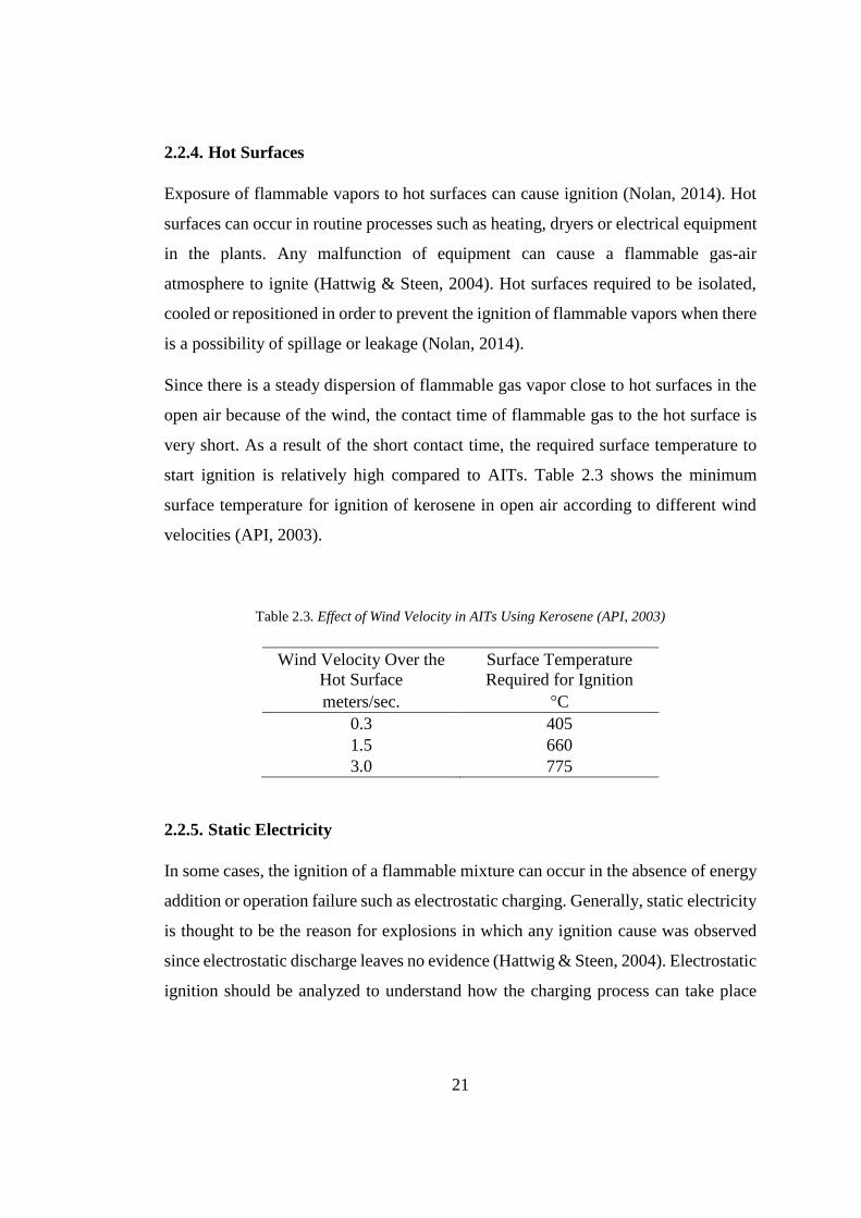
start ignition is relatively high compared to AITs. Table 2.3 shows the minimum

surface temperature for ignition of kerosene in open air according to different wind

velocities (API, 2003).

Table 2.3. Effect of Wind Velocity in AITs Using Kerosene (API, 2003)

Wind Velocity Over the

Hot Surface

Surface Temperature

Required for Ignition

meters/sec. °C

0.3 405

1.5 660

3.0 775

2.2.5. Static Electricity

In some cases, the ignition of a flammable mixture can occur in the absence of energy

addition or operation failure such as electrostatic charging. Generally, static electricity

is thought to be the reason for explosions in which any ignition cause was observed

since electrostatic discharge leaves no evidence (Hattwig & Steen, 2004). Electrostatic

ignition should be analyzed to understand how the charging process can take place

22

and to find out the location of the accumulation of static electricity (Lüttgens et al.,

2017).

Electrostatic charge can ignite combustible vapors as a result of the same sequence of

physical processes shown in Figure 2.5.

Figure 2.5. Ignition Process of Flammable Vapors by Electrostatic Electricity (Hattwig & Steen,

2004)

Even if the ignition process looks simple, it is very hard to define each step on the

field since many different operations are conducted at the same time. Therefore,

electrostatic charge accumulation is correspondent to the overall rate of charge

separation and discharge.

In industrial plants, movement of conveyor belts, vehicle transportation and walk of

workers on the insulating ground can cause electrostatic charge accumulation. It is

23

vital to notice that after the contact process, all surfaces which are in contact with each

other are charged.

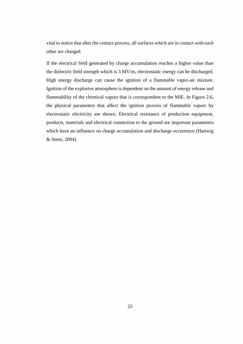
If the electrical field generated by charge accumulation reaches a higher value than

the dielectric field strength which is 3 MV/m, electrostatic energy can be discharged.

High energy discharge can cause the ignition of a flammable vapor-air mixture.

Ignition of the explosive atmosphere is dependent on the amount of energy release and

flammability of the chemical vapors that is correspondent to the MIE. In Figure 2.6,

the physical parameters that affect the ignition process of flammable vapors by

electrostatic electricity are shown. Electrical resistance of production equipment,

products, materials and electrical connection to the ground are important parameters

which have an influence on charge accumulation and discharge occurrence (Hattwig

& Steen, 2004).

24

Figure 2.6. The Physical Parameters Affecting the Ignition Process of Flammable Vapors by

Electrostatic Electricity (Hattwig & Steen, 2004)

2.3. JP-8 and Kerosene

Unrefined form of petroleum has a very limited range of direct use in industrial areas.

Oil gains value after being transformed into commercial products in the refineries

(Speight & El-Gendy, 2018). Liquid petroleum products can vary from highly volatile

naphtha to lubricant oils which have very low volatility (Speight, 2014). Generally,

physical characteristics are used to categorize liquid petroleum products (Speight &

El-Gendy, 2018).

25

Kerosene (kerosine can also be used) is one of the liquid, colorless and flammable

petroleum product with specific odor. It is commonly used for burning lamps, heating

houses, fueling jet engines, solvent for greases and insecticides. In general, the term

kerosene is wrongly used for describing fuel oils however fuel oil can be any type of

liquid petroleum by-product which is used to obtain heat or power when burned

(Speight & El-Gendy, 2018).

Table 2.4. Petroleum Products (Speight & El-Gendy, 2018)

Product

Lower

Carbon

Limit

Upper

Carbon

Limit

Lower Boiling

Point (°C)

Upper

Boiling Point

(°C)

Refinery gas C1 C4 -161 -1

Liquefied petroleum

gas

C3 C4 -42 -1

Naphtha C5 C17 36 302

Gasoline C4 C12 -1 216

Kerosene/diesel fuel C8 C18 126 258

Aviation turbine fuel C8 C16 126 287

Fuel oil C12 >C20 216 421

Lubricating oil >C20 >343

Wax C17 >C20 302 >343

Asphalt >C20 >343

Coke >C50 >1000

Kerosene is a chemical mixture of hydrocarbons. Constituents of kerosene vary

according to their source. Mostly, kerosene contains various hydrocarbons with 10 to

16 carbon atoms (Speight, 2011). Table 2.4. shows carbon numbers of various

petroleum products. Ghassemi et al. (2006) say that kerosene has very similar general

properties to dodecane, C12H26. Table 2.5. demonstrates average formula of petroleum

products. According to Chickos and Hanshaw (2004), enthalpy of vaporization of

dodecane is 65.1 kJ/mol. Dodecane has a boiling temperature of 216 °C (Safety Data

Sheet (SDS) – Thermo Fisher Scientific, 2018). Kerosene is more volatile than diesel

oil but not more volatile than gasoline. Kerosene can be distilled between 150-300 °C.

Flash point of kerosene is around 25 °C (Speight & El-Gendy, 2018).

26

Table 2.5. Assumed Average Formula of Petroleum Fuels (Totten et al., 2003)

Fuel Assumed Average Formula

Aviation gasoline C7.3H15.3

Aviation kerosene C12.5H24.4

Gas oil C15H27.3

Kerosene is mainly used as jet fuel in aviation. Some particular characteristics are

needed to be used as aviation fuel such as high flash point for safe handling, low

freezing point for cold weather usage and no mixing with water. Table 2.6 shows the

heat of vaporization values for several oil products (Speight, 2017).

Table 2.6. Heat of Vaporization of Oil Products (Speight, 2017)

Product Gravity, °API Average boiling

temp, °F

Heat of vaporization

Btu/lb* Btu/gal*

Gasoline 60 280 116 715

Naphtha 50 340 103 670

Kerosene 40 440 86 595

Fuel oil 30 580 67 490

*Btu/lb × 2.328 = kJ/kg; Btu/gal × 279 = kJ/M3

Jet fuel is light petroleum distillate and has different types for usage in jet engines.

Commonly used jet fuels for military purposes are JP-4, JP-5, JP-6, JP-7 and JP-8. JP-

8 is kerosene modeled fuel which is also used in civil aviation (Speight & El-Gendy,

2018). According to the U.S. Department of Defense (2015), JP-8 is a kerosene-type

engine fuel which contains several additives such as fuel system corrosion and icing

inhibitors.

Mainly, straight alkanes, branched alkanes and cycloalkanes are present in aviation

fuels. A maximum of 20%–25% of fuel consist of aromatic hydrocarbons since they

cause smoke after combustion. 5% of total fuel is limited to alkenes for JP-4.

Approximately, the percentage of ingredients of aviation fuel are 32% of straight-

27

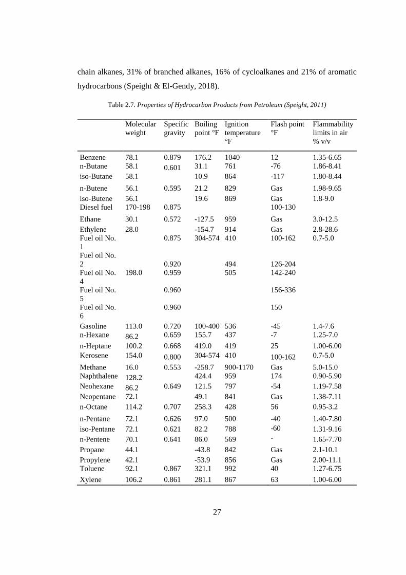
chain alkanes, 31% of branched alkanes, 16% of cycloalkanes and 21% of aromatic

hydrocarbons (Speight & El-Gendy, 2018).

Table 2.7. Properties of Hydrocarbon Products from Petroleum (Speight, 2011)

Molecular

weight

Specific

gravity

Boiling

point °F

Ignition

temperature

°F

Flash point

°F

Flammability

limits in air

% v/v

Benzene 78.1 0.879 176.2 1040 12 1.35-6.65

n-Butane 58.1 0.601 31.1 761 -76 1.86-8.41

iso-Butane 58.1 10.9 864 -117 1.80-8.44

n-Butene 56.1 0.595 21.2 829 Gas 1.98-9.65

iso-Butene 56.1 19.6 869 Gas 1.8-9.0

Diesel fuel 170-198 0.875 100-130

Ethane 30.1 0.572 -127.5 959 Gas 3.0-12.5

Ethylene 28.0 -154.7 914 Gas 2.8-28.6

Fuel oil No.

1

0.875 304-574 410 100-162 0.7-5.0

Fuel oil No.

2

0.920

494 126-204

Fuel oil No.

4

198.0 0.959 505 142-240

Fuel oil No.

5

0.960 156-336

Fuel oil No.

6

0.960 150

Gasoline 113.0 0.720 100-400 536 -45 1.4-7.6

n-Hexane 86.2 0.659 155.7 437 -7 1.25-7.0

n-Heptane 100.2 0.668 419.0 419 25 1.00-6.00

Kerosene 154.0 0.800 304-574 410 100-162 0.7-5.0

Methane 16.0 0.553 -258.7 900-1170 Gas 5.0-15.0

Naphthalene 128.2 424.4 959 174 0.90-5.90

Neohexane 86.2 0.649 121.5 797 -54 1.19-7.58

Neopentane 72.1 49.1 841 Gas 1.38-7.11

n-Octane 114.2 0.707 258.3 428 56 0.95-3.2

n-Pentane 72.1 0.626 97.0 500 -40 1.40-7.80

iso-Pentane 72.1 0.621 82.2 788 -60 1.31-9.16

n-Pentene 70.1 0.641 86.0 569 - 1.65-7.70

Propane 44.1 -43.8 842 Gas 2.1-10.1

Propylene 42.1 -53.9 856 Gas 2.00-11.1

Toluene 92.1 0.867 321.1 992 40 1.27-6.75

Xylene 106.2 0.861 281.1 867 63 1.00-6.00

28

The most important characteristics for kerosene are flash point, fire point and boiling

range. The flash point of kerosene is generally set above the average ambient

temperature. The fire point is essential for determining fire prevention means. The

distillation range is not a significant property however it can be seen as an indicator

of viscosity. Additionally, pureness of the kerosene can be understood by the steady

burning of the product over a time interval (Speight, 2011). Table 2.7. shows several

properties of hydrocarbon products.

ACGIH (2015) states that kerosene/jet fuels, as total hydrocarbon vapor, have TLV-

TWA of 200 mg/m3. Additionally, exposures above the TLV-TWA value should not

be allowed for more than 15 minutes. Kerosene has TLV –TWA of 30 ppm and an

odor threshold of 0.1 ppm. Additionally, kerosene has a lower explosion limit (LEL)

of 0.7% and an upper explosion limit (UEL) of 5% by volume. (Material Safety Data

Sheet (MSDS) – John Duffy Energy Services, 2006)

According to the U.S. Department of Defense (2015), kerosene-type aviation turbine

fuel, JP-8 should comply with the requirements given in the military standard MIL-

DTL-83133J. Table 2.8 shows some requirements of MIL-DTL-83133J.

Table 2.8. Chemical and Physical Requirement (U.S. Department of Defense, 2015)

Property Min Max

VOLATILITY

Distillation temperature, °C

Initial boiling point

10 percent recovered 205

20 percent recovered

50 percent recovered

90 percent recovered

Final boiling point 300

Residue, vol percent 1.5

Loss, vol percent 1.5

Flash point, °C 38

Density

Density, kg/L at 15 °C or 0.775 0.840

Gravity, API at 60 °F 37.0 51.0

29

2.4. Fuel Servicing of Aircraft

Aircraft fuel servicing is the process of transfer of fuel to or from a fuel supply to or

from an aircraft together with fueling connection and disconnection operation. Fueling

operation supervisor must confirm that all fuel servicing operators are capable of

conducting fueling operation safely by following technical orders under their

supervision (USAF, 2013).

2.4.1. Electrostatic Hazards in Fuel Servicing and Static Grounding and Bonding

Aircraft fuel does not burn in liquid form but it burns in the gaseous state. Volatility

is the ability of a liquid to transform into gaseous form and fuel can vaporize at low

temperatures. Therefore, gaseous or vapor form of fuel has fire and explosion hazards

during fuel servicing of aircraft (FAA, 2008).

Static electricity can be described as a buildup of electric charge on the uppermost

layer of material (Wang, 2019). Static electricity can be formed by friction of two

materials. Fuel flow inside a fueling pipeline generates electrostatic charging.

Additionally, the structural frame of the aircraft accumulates static electricity due to

friction in the air during the flight. Static electricity should be discharged before

fueling operation otherwise, it reaches to ground through fueling pipeline and it can

cause the ignition of fuel vapors.

There is always a hazard of fire and explosion due to electrostatic charges in fuel

servicing of aircraft. The most effectual way of preventing electrostatic hazards is

grounding or bonding. Grounding is the connection of metallic materials to ground.

Bonding is the connection of two or more metallic materials to each other by a

conductor to equalize electrostatic potential (FAA, 2008).

While filling the fuel tank, the electrical potential of fuel flow can increase up to

thousands of volts. A spark discharged from pipelines, fittings or any other object can

30

ignite fuel vapor-air mixture. Any contaminant object in the fuel tank will accumulate

the electrostatic charge and act as an electrical condenser. The potential needed for

discharging from contaminant to fuel is much less than the amount necessary for

discharge from fuel to tank. As a result, contamination of fuel dramatically increases

the electrostatic hazards. If the fuel flow is kept under the allowable fueling rates,

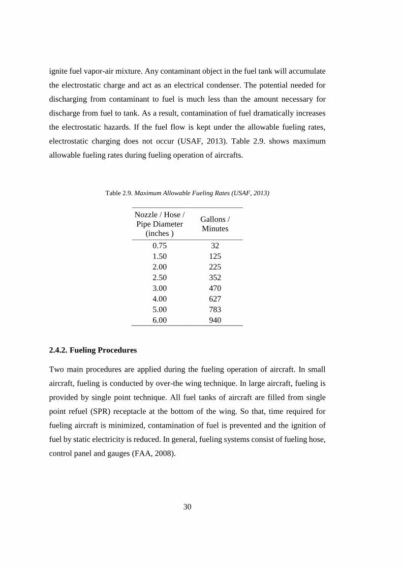
electrostatic charging does not occur (USAF, 2013). Table 2.9. shows maximum

allowable fueling rates during fueling operation of aircrafts.

Table 2.9. Maximum Allowable Fueling Rates (USAF, 2013)

Nozzle / Hose /

Pipe Diameter

(inches )

Gallons /

Minutes

0.75 32

1.50 125

2.00 225

2.50 352

3.00 470

4.00 627

5.00 783

6.00 940

2.4.2. Fueling Procedures

Two main procedures are applied during the fueling operation of aircraft. In small

aircraft, fueling is conducted by over-the wing technique. In large aircraft, fueling is

provided by single point technique. All fuel tanks of aircraft are filled from single

point refuel (SPR) receptacle at the bottom of the wing. So that, time required for

fueling aircraft is minimized, contamination of fuel is prevented and the ignition of

fuel by static electricity is reduced. In general, fueling systems consist of fueling hose,

control panel and gauges (FAA, 2008).

31

There are several precautions in order to prevent fire and explosion hazards during the

fueling operation. Firstly, all electrical devices and electronic systems, including

radar, must be closed down during fueling operation. Aircraft and fueling equipment

must be grounded. Proper type of fire extinguishers must be available. Fueling

operators are not allowed to carry any kind of equipment that can produce flame. The

operator must wear antistatic safety shoes, clothes and eye protection (FAA, 2008).

Operators shall carry a dead man control unit in order to stop fuel flow in case of

emergency. Service operator shall report any type of probable hazard such as fuel

leakage, spillage or spray, fault bonding/grounding of receptacles, visible spark from

any source to the supervisor immediately.

Housekeeping of the work area is an important issue in aviation. Clean and tidy

workplace is necessary for safe and effective operations in fueling stations, aircraft

parking areas and servicing aprons. Safe fuel servicing can be provided by the

prevention of fuel spills and removing ignition sources from fuel servicing stations.

Fuel servicing safety zone (FSSZ) must be established and retained during fueling

operations. FSSZ covers 50 feet radius area centering fuel servicing components such

as SPR, and 25 feet around fuel vent outlets. Figure 2.7 shows an example of a fuel

servicing safety zone (FSSZ). Another aircraft next to FSSZ can keep its engine

running as long as its thrust is not directed toward FSSZ (USAF, 2013). Throughout

the fuel servicing of aircraft, all possible ignition sources such as ground servicing

equipment are eliminated and kept away from FSSZ. Servicing equipment must be

positioned so a clear path is maintained to allow fast evacuation of vehicles and staff

in an emergency (USAF, 2018).

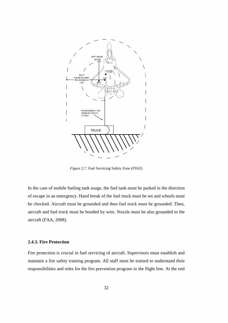
32

Figure 2.7. Fuel Servicing Safety Zone (FSSZ)

In the case of mobile fueling tank usage, the fuel tank must be parked in the direction

of escape in an emergency. Hand break of the fuel truck must be set and wheels must

be chocked. Aircraft must be grounded and then fuel truck must be grounded. Then,

aircraft and fuel truck must be bonded by wire. Nozzle must be also grounded to the

aircraft (FAA, 2008).

2.4.3. Fire Protection

Fire protection is crucial in fuel servicing of aircraft. Supervisors must establish and

maintain a fire safety training program. All staff must be trained to understand their

responsibilities and roles for the fire prevention program in the flight line. At the end

33

of every shift, field inspection should be carried out to ensure that there is no fire risk

in the flight line (USAF, 2018). Supervisor should give briefing on emergency action

plan to servicing operators before fueling service. The fire department must be notified

before the fuel servicing operation (USAF, 2016). In case of fire or fuel leakage, fuel

servicing operators are the first team of defense. Servicing operators must alert the fire

department immediately and use available firefighting equipment until the fire

department reaches to the area.

Fueling operation supervisor should ensure the proper type of fire extinguisher for fire

class is available in the fuel servicing area. Fueling area fire extinguisher should be

kept in a vertical position in order to increase firefighting effectiveness. Putting down

fire extinguisher causes it to be unavailable to discharge all of its agents. The fire

extinguishers should be used only for the initial knockdown of fire.

During the fueling operation in hangars, two fire extinguishers must be available

within 100 feet of the hangar. The wheeled 150-pound Halon 1211 or Novec 1230

must be used as fire extinguishers in the hangars. Fire extinguishers must be replaced

outside of 25 feet radius safety zone of the aircraft fuel vent outlet during fuel servicing

of aircraft (USAF, 2013).

Supervisors must be sure of all fire extinguishers are inspected on a monthly basis and

inspection records are documented. Extinguishers with nonconformity must be taken

out of service and they must be replaced immediately. Fire extinguishers must be in

designated points in the flight line. There must be no obstacles for access and visibility

to fire extinguishers. The safe seal of fire extinguisher must be in place and not be

deformed. The pressure gauge must be in the operable range. All staff must have

knowledge about the fire alarm system, reporting an emergency and activation of the

alarm system (USAF, 2018).

Warning signs must be hanged in visible places in the fueling area. Smoking and its

materials are forbidden within the fuel servicing area and 6 m radius area around

fueling systems (NFPA, 2003a).

34

Water suppression systems are not effective for fuel spillages. Water causes

surrounding materials to become cooler however it also causes to spread of pool fire.

In the case of a large amount of fuel spills, the drainage system is useful for mitigating

the spread of burning fuels. The sprinkler system can be considered to be installed

inside the drain system (NFPA, 2003b).

2.5. Modeling JP-8 Evaporation

Evaporation modeling is the most important subject for JP-8 spillage. All JP-8 spills

include the evaporation process. However, the researches which have been carried out

so far are insufficient to understand important concepts of oil spillage evaporation

modelling (Fingas, 2013). It is very important to understand the evaporation process

of oil to make an accurate prediction of evaporation rates of oil products in the case

of oil spills (Fingas, 1995). The evaporation process can be described as the

transformation of molecules from the liquid phase to the vapor phase under the boiling

temperature of a substance. The kinetic energy of a liquid molecule is enough for

moving away from the liquid surface to the vapor phase (Schaschke, 2014). In other

words, the evaporation process can be described as liquid molecule movement from

the liquid surface to the vapor phase. The air layer on the liquid surface is described

as air boundary layer which has a thickness of less than 1 mm (Fingas, 2013). In

general, the boundary layer can be described as a layer in a liquid where transfer

activity is affected by characteristics of the surface below (Monteith and Unsworth,

2013). The most important concern about the air boundary layer is that it can affect

the evaporation process. For the water evaporation process, the air boundary layer has

an influence on the evaporation rate (Fingas, 2013). According to Fingas (2001), the

oil evaporation rate is mainly dependent on the chemical composition of the oil

compound. On the other hand, Haghighi et al. (2013) state that besides interior

limitations, the air boundary layer has a restriction on the evaporation ratio of liquid

substances. Some amount of water vapor can be held by air which is described as

35

relative humidity. If there is no wind and the air layer doesn’t have movement, the

water evaporation rate decreases since the air layer above the water is saturated. As a

result, it can be said that the mechanism of water evaporation is regulated by the air

boundary layer. Then, in the presence of wind, the evaporation rate of water is

expected to increase (Fingas, 2013). On the other hand, most of the liquids which have

air boundary layer evaporation regulation, evaporate very slowly to saturate the air

boundary layer on the top of the surface (Fingas, 2011b).

On the contrary, the evaporation mechanism of some liquids are not regulated by air-

boundary-layer since the evaporation rate is very slow for saturation of the air layer

above the liquid. According to Fingas (2013), there are some liquids which have an

evaporation mechanism regulated by molecular diffusion. Oil and fuels have diffusion

regulated evaporation process since they consist of many different liquid compounds.

As a result, the evaporation process of oils is not significantly influenced by increased

spill area and wind velocity. The evaporation rate of water is linear with time since it

is a single compound. On the other hand, oil products do not have a linear evaporation

rate with respect to time (Fingas, 1997).

2.5.1. Historical Development of Oil Evaporation Modeling

According to Fingas (2011a), for liquids with air-boundary-layer evaporation model

can be written as:

𝐸 ≈ 𝐾 𝐶 𝑇𝑢 𝑆 (1)

In equation (1), E represents evaporation rate in mass/unit area, K represents mass

transfer rate of evaporated fluid, C represents the concentration (mass/volume) of

evaporated fluid, Tu is relative intensity factor of turbulence and S is the saturation

factor (Fingas, 2013). As air above the liquid becomes more saturated evaporation rate

of the liquid decreases (Fingas, 1998).

36

According to Fingas (1999), Sutton was one of the pioneers of the oil evaporation

study. Fingas (2013) says that Sutton formed a model according to experimental data:

𝐸 = 𝐾 𝐶 𝑈7 9⁄ 𝑑𝑎−1 9⁄

𝑆𝑐−𝑟 (2)

In equation (2), C represents the concentration of the evaporated liquid as mass per

volume, U represents the velocity of wind, da is the pool area, Sc represents Schmidt

number and r represents the experimental value between 0 and 2/3. The parameters in

equation (2) are very similar to ones in equation (1). In equation (2), turbulence is

described as multiplication of wind velocity, U, and Schmidt number, Sc (Fingas,

2013). Schmidt number can be found by theoretical study and empirical methodology

(Yuan et al., 2017). Fingas (2013) states that the evaporation rate for oil was

theoretically formulated for the first time by Blokker. Blokker assumed oil as a single

component fluid. Distillation values and boiling points of all different liquid

components in oil are provided to make an assumption on average vapor pressure. The

Clausius-Clapeyron equation was used to calculate overall vapor pressure of oil

components in the form as:

log𝑃𝑠

𝑃=

∆𝑣𝑎𝑝𝐻0 M

4.57(

1

T−

1

𝑇𝑠) (3)

In equation (3), P represents vapor pressure at T which is absolute pressure, Ps (760

mm Hg) represents vapor pressure at boiling point, Ts, ∆𝑣𝑎𝑝𝐻0 is the heat of

evaporation as cal/g and M is the molecular weight.

According to Fingas (2013), ∆𝑣𝑎𝑝𝐻0M/(4.57 Ts) was considered as a constant value

for hydrocarbons. Hence, the equation became as:

log 𝑃𝑠 𝑃 = 5.0[(𝑇𝑠 − 𝑇) 𝑇⁄ ]⁄ (4)

The pressure curve was obtained by using equation (4) and experimental data. In this

calculation, Raoult’s law was assumed to be valid providing that ∆𝑣𝑎𝑝𝐻0M is a

function of evaporation percentage. Overall evaporation time was found by

application of Pasquill’s equation as:

37

𝑡 =∆ℎ 𝐷𝛽

𝐾𝑒𝑣 𝑈𝛼∑

1

𝑃𝑀 (5)

In equation (5), t represents total evaporation time in hours, ∆ℎ signifies a drop in

thickness of layer in meters, D symbolizes oil spill diameter, 𝛽 represents a

meteorological coefficient (valued as 0.11), 𝐾𝑒𝑣 signifies atmospheric stability

coefficient value given as 1.2x10-8, 𝛼 symbolizes a meteorological coefficient (valued

as 0.78), P symbolizes the vapor pressure at absolute temperature (T) and M represents

the molecular weight of the liquid. According to Fingas (2013), the results of equation

(5) were not in correlation with data collected from the experiment conducted in a

wind tunnel.

According to Jenkins (2008), The Clausius–Clapeyron equation can be expressed as:

ln (𝑃2

𝑃1) = − (

∆𝑣𝑎𝑝𝐻0

𝑅) [

1

𝑇2−

1

𝑇1] (6)

If the exponential of the equation (6) is taken, then the equation yields a different form

of the Clausius-Clapeyron equation such as (Jenkins, 2008):

(𝑃2

𝑃1) = 𝑒𝑥𝑝 {− (

∆𝑣𝑎𝑝𝐻0

𝑅) [

1

𝑇2−

1

𝑇1]} (7)

Fingas (2013) states that Mackay and Matsugu worked on oil evaporation modelling

by combining the water evaporation model and empirical data. The model used for

water evaporation was modified for oils by using the evaporation data of cumene. To

formalize oil evaporation rate, evaporation rate of water and cumene were correlated

as a wind velocity and pool areas function given the equation (Mackay & Matsugu,

1973):

𝐾 = 𝑐 𝑈0.78𝑋−0.11 (8)

In order to obtain a constant value for equation coefficient c, Mackay and Matsugu

observed evaporation of cumene for more than two days. Schmidt number is taken as

2.70 for cumene evaporation. It is important to notice that the dimension of c changes

caccording to units used for mass transfer constant, K, wind velocity, U and pool

38

diameter, X which are m/h, m/h and m respectively. In the case of evaporation

modelling different than cumene, a value of 0.0292 Sc-0.67 can be used. Therefore, the

equation (8) yields to (Mackay & Matsugu, 1973):

𝐾 = 0.0292 𝑈0.78𝑋−0.11𝑆𝑐−0.67 (9)

According to Fingas (2013), Mackay and Matsugu say oil evaporation has complexity

since there is a diffusion resistance of oil molecules. Empirical data on the oil

evaporation rate was not in correlation with the results of calculated data which means

diffusion resistance occurs. As a result, mass transfer constant is needed to model oil

evaporation in spillages. The amount of evaporation of an oil spill in an environment

can be determined by mass transfer constant (Goodwin et al., 1973). In order to test

mass transfer constant methodology, Butler studied on an evaporation equation with

mass transfer data available for specific conditions. In Butler’s model evaporation is

proportional to vapor pressure, P as shown :

𝑑𝑥 𝑑𝑡 = −𝑘𝑃(𝑥 𝑥0⁄ )⁄ (10)

In equation (10), x represents the amount of specific oil product at time t, xo

symbolizes the amount of specific oil product at time t equals zero, k signifies

experimental rate constant and P represents the vapor pressure of specific oil product

(Fingas, 2013).

Butler also thought that P cannot represent the overall vapor pressure of the spillage

since oil consists of various components. Also, there would not be big changes in

activity constant during weathering. Accordingly, activity constants were included in

the experimental rate constant k. For various oil products, P and k were considered as

independent of the amount, x. As a result, the equation was derived to yield amount

remaining after evaporation as:

𝑥 𝑥0 = 𝑒𝑥𝑝(−𝑘𝑡𝑃 𝑥0⁄ )⁄ (11)

After that, the regression line was used to predict model for vapor pressure of a single

oil product:

39

𝑃 = 𝑒𝑥𝑝(10.94 − 1.06 𝑁) (12)

In equation (12), P is the vapor pressure in Torr and N is the carbon number of oil

product. Then, equations (11) and (12) were combined given the formula:

𝑥 𝑥0 = 𝑒𝑥𝑝[−(𝑘 𝑡 𝑥0⁄ ) 𝑒𝑥𝑝(10.94 − 1.06 𝑁)]⁄ (13)

According to the equation (13), the weathered oil amount is formulated as a function

of carbon number of oil product, N. If oil components are distributed uniformly, the

equation (13) can estimate carbon number as a function of time where the known

amount evaporated (x = 0.5 xo):

𝑁1 2⁄ = 10.66 + 2.17 log 𝑘𝑡 𝑥0⁄ (14)

The model was applied to some oil spills whose time of occurrence is known and the

results were compared. The age prediction of the oil spill made by the equation was

accurate. According to Fingas (2013), the equation was valid for water spillages also,

but it was never preferred in modelling.

According to Fingas (2013), Mackay and Matsugu diffusion model is used by Yang

and Wang to develop an evaporation model. Molecular diffusion is described as:

𝐾 =𝑘𝑚(𝑃𝑖−𝑃𝑖∞)

[𝑅 𝑇𝑠] (15)

In equation (15), 𝐾 represents mass transfer rate, 𝑘𝑚 symbolizes a constant which

involves all factors related to 𝐾, 𝑃𝑖 signifies vapor pressure of oil compound, I, on the

boundary, 𝑃𝑖∞ signifies the vapor pressure of oil compound, I, at infinite altitude of

the atmosphere, R represents molar gas constant and 𝑇𝑠 absolute temperature of the

oil layer on water. Yang and Wang (1977) also suggest the equation below:

𝐾 = 𝑎 𝐴𝛾𝑒𝑞𝑈 (16)

In equation (16), A is the area of oil layer on water, U is the wind velocity and a, q

and 𝛾 are experimental constants. Fingas (2013) says that research results indicated

that, in the process of oil evaporation a surface film is formed on the oil layer, and it

40

caused an evaporation process to slow down. Before the film has formed on the oil

layer (ϱt/ϱo < 1.0078):

𝐾𝑚𝑏 = 69 𝐴−0.0055 𝑒0.42𝑈 (17)

In equation (17), 𝐾𝑚𝑏 represents the constant which includes all factors concerning oil

evaporation before the surface film. After the film has formed (ϱt/ϱo > 1.0078):

𝐾𝑚𝑎 = 1 5⁄ 𝑘𝑚𝑏 (18)

For equation (18), ϱo represents initial oil density, ϱt symbolizes oil density at time t

and 𝐾𝑚𝑎 is the coefficient which includes all factors concerning oil evaporation after

the surface film. According to Fingas (2013), research results showed that the film

formed on the surface of the oil causes five times lower evaporation rate.

According to Drivas (1982), the model defined by Mackay and Matsugu has good

accuracy to predict oil evaporation compared to the empirical data available in the

literature. Reijnhart and Rose (1982) studied an equation to predict oil evaporation at

sea level. Reijnhart and Rose model was as:

𝐸 = 𝛼1 𝑐0 (19)

In equation (19), 𝐸 symbolizes evaporation rate of oil compound, 𝛼1 represents

coefficient which is the combination of wind speed and all factor in m/s and 𝑐0

signifies the equilibrium concentration of vapor at the top layer of the oil (Reijnhart

and Rose, 1982). According to Fingas (2013), research was conducted to compare test

data and evaporation rates on the sea level. However, there is not a specific

methodology to estimate equilibrium concentration, 𝐶0.

According to Fingas (2013), Brighton redefined evaporation equation, and he studied

on water evaporation with a similar approach to Sutton as:

𝐸 = 𝐾 𝐶𝑠 𝑈7/9 𝑑1−1/9 𝑆𝑐−𝑟 (20)

41

In equation (20), E represents evaporation rate per unit area, 𝐾 symbolizes

experimental mass transfer coefficient, 𝐶𝑠 signifies evaporating liquid concentration,

d1 represents pool length and r symbolizes an experimental constant value between 0

and 2/3.

Brighton (1985) states that evaporating liquid concentration, 𝐶𝑠, can be determined by

the formula:

𝐶𝑠 =𝑀 𝑃𝑣

𝑅 𝑇 (21)

In equation (21), 𝑀 is the molecular weight of the substance, 𝑃𝑣 represents saturated

vapor pressure, T is temperature and R is the gas constant.

According to Fingas (2013), Brighton thought that the formula can also comply with

the fundamental dimensionless form including wind velocity, U, and roughness

length, Z0, which describes air-boundary-layer phenomena. In Brighton’s analysis

concentration is logarithmic above the surface which can be thought to be a more ideal

approach than the results previously obtained. Brighton (1985) used a power profile

for the estimation of turbulence, so the parameters above can be replaced into the

equation:

𝑈 =𝑢∗

𝑘 𝑛 (22)

𝑛 = (ln𝑧1

𝑧0) (23)

In equation (22), 𝑢∗ represents friction velocity, 𝑧1 signifies height above the surface,

𝑧0 symbolizes roughness length and n represents the power law dimensionless

parameter. When the equations (22) and (23) were substituted into the evaporation

model, the obtained equation was:

𝑈 (𝑧

𝑧1)

𝛿𝑦

𝛿𝑋=

𝛿

𝛿𝑧(

𝑘 𝑢∗ 𝑧

𝑆𝑐) (

𝛿𝐶

𝛿𝑧) (24)

42

In equation (24), z represents height above the surface, C symbolizes concentration of

evaporated oil product, X is the size of the pool, k signifies von Karman coefficient

obtained by K/u* z and 𝑆𝑐 represents the Schmidt number which was assumed as 0.85.

The results of Brighton’s model were evaluated and it was decided that some

experimentation concluded with good results, however, data was not enough for

testing the theory and control of the operation environment was poor (Brighton, 1990).

Fingas (2013) says that Tkalin described an evaporation model for oil at sea level as:

𝐸𝑖 =𝐾𝑀𝑃𝑜𝑖 𝑥

𝑅𝑇 (25)

In equation (25), 𝐸𝑖 represents evaporation rate of oil compound i or total evaporation

in kg/m2s, K symbolizes mass transfer constant in m/s, M signifies molecular weight,

Poi represents vapor pressure of the oil compound i and x signifies the amount of the

oil product i at time t. Experimental data was used to define parameters in the model:

𝑃𝑜𝑖 = 103𝑒𝐴 (26)

In equation (26), A was described as:

𝐴 = −(4.4 + log 𝑇𝑏)[1.803 {𝑇𝑏 𝑇⁄ − 1} − 0.803 ln(𝑇𝑏 𝑇⁄ )] (27)

In equation (27), Tb represents the boiling point of the oil product. Mass transfer

constant was described as:

𝐾 = 1.25 𝑈 10−3 (28)

According to Fingas (2013), Tkalin model for oil evaporation was confirmed by

experimental results obtained from the literature.

Stiver and Mackay (1984) formulated an evaporation model, which is modified from

Mackay and Matsugu’s equation, is one of the most commonly used approach in oil

spills. In the model, it was assumed that an oil is spilled and the evaporation rate was

defined as:

𝐸 = 𝐾𝐴𝑃 (𝑅𝑇)⁄ (29)

43

In equation (29), E represents the evaporative molar flux in mol/s, K symbolizes mass

transfer constant under the wind effect in ms-1, A represents the area in square meters,

P symbolizes vapor pressure of the liquid as Pascal and T is the temperature as degree

Kelvin. The equation was rearranged as:

𝑑𝐹𝑣 𝑑𝑡⁄ = 𝐾 𝐴 𝑃 𝑣 (𝑉0 𝑅 𝑇)⁄ (30)

In equation (30), Fv represents the volume of the evaporated compound, v symbolizes

the molar volume of the liquid in m3/mol and V0 signifies the volume of the spillage

at the beginning in m3. Then, equation (30) yields:

𝑑𝐹𝑣 = [𝑃 𝑣/(𝑅 𝑇)](𝐾 𝐴 𝑑𝑡/𝑉0) (31)

which was arranged to give:

𝑑𝐹𝑣 = 𝐻 𝑑𝜃 (32)

In equation (32), H represents Henry’s law constant, and 𝜃 symbolizes evaporative

exposure (Stiver and Mackay, 1984). In equation (31), (𝐾 𝐴 𝑑𝑡/𝑉0) signifies the time-

rate of evaporative exposure and was represented as 𝑑𝜃 in equation (32). As it can be

seen from the equation, the evaporative exposure is correspondent to time, area of

spillage, the thickness of oil spill and mass transfer constant which is a function of the

wind velocity. In other words, the evaporative exposure can be seen as the vapor

volume ratio to initial fluid volume.

In equation (31), [𝑃 𝑣/(𝑅 𝑇)] signifies H in equation (32) and H represents Henry’s

law constant. H is correspondent to temperature. Hence, 𝜃𝐻 represents the ratio of the

amount of oil evaporated to the initial amount. In the case of pure fluids, H can be

assumed as independent to Fv so equation (30) was rearranged as (Fingas, 2013):

𝐹𝑣 = 𝐻 𝜃 (33)

According to Fingas (2013), when K, A and temperature do not vary, the evaporation

rate does not vary too, and the evaporation process can be thought as finished if 𝜃 gets

to the level of 1/H.

44

In the case of fluid involving multiple compounds, H can be assumed as dependent on

Fv. Therefore, H should be defined by using Fv to rearrange equation (31), that is, the

vapor pressure variable can be described as a correlation with composition. In this

situation, evaporation of the oil decreases as evaporation continues. Fingas (2013)

says that equation (31) was rearranged by experimental data to obtain:

𝐹𝑣 = (𝑇 𝐾1⁄ ) ln(1 + 𝐾1𝜃 𝑇⁄ ) 𝑒𝑥𝑝(𝐾2 − 𝐾3 𝑇⁄ ) (34)

In equation (34), Fv represents the ratio of the volume evaporated and K1, 2, 3

symbolizes experimental coefficients. K1 was found from the slope of the curve of Fv

versus log 𝜃 by evaporation experiments. According to Fingas (2013), when 𝜃 is

bigger than 104, the value of K1 approaches the value of 2.3T divided by the slope. K2

and K3 were found separately by evaporation curvature at two different temperatures.

Fingas (2013) says that Hamoda and co-workers also studied evaporation in theory

and conducted empirical researches. An approach was developed to understand how

American Petroleum Institute gravity, APIo (expression for density), temperature and

salinity affect mass transfers constant, K (Hamoda et al., 1989):

𝐾 = 1.68 × 10−5 (𝐴𝑃𝐼°)1.253 (𝑇)1.80 𝑒−0.1441 (35)

In equation (35), K represents mass transfer constant in cm/h, 𝐴𝑃𝐼° symbolizes

unitless density API parameter, and T signifies temperature as degree Celsius.

Exponential values in the model were found from the results obtained from the

experiments after multiple linear regression (Hamoda et al., 2013).

Quinn et al. (1990) provided an oil spill to make it evaporate in a conditioned medium

and compared the evaporation records with former models such as Fick’s diffusion

law and the Clausius-Clapeyron equation. In this study, oil was separated into different

components according to their boiling point. Every component was regarded as equal

to an n-paraffin. Fractions of n-paraffin were decided by capillary gas-liquid

chromatography. The evaporation rate in the field and evaporation rates obtained by

45

modelling were compared. Evaporative modelling gives very accurate results for film

thickness from 10 µm to 1 mm until 4 weeks of weathering.

Bobra (1992) worked on oil evaporation modeling. The evaporation rates of different

oil components were observed in numerous weathering conditions. The data collected

from observations were evaluated regarding the formula given by Stiver and Mackay

(1984). The formula was:

𝐹𝑉 = ln[1 + 𝐵(𝑇𝐺 𝑇⁄ ) 𝜃 𝑒𝑥𝑝(𝐴 − 𝐵 𝑇0 𝑇⁄ )] {𝑇 𝐵𝑇𝐺⁄ } (36)

In equation (36), FV represents the ratio evaporated, TG symbolizes the slope of the

distillation curvature, A and B signifies unitless coefficients, T0 is the boiling point of

the oil product at the beginning and 𝜃 represents evaporative exposure. In order to

understand the effectiveness of the model, empirical data and modeling results were

compared where results were found to be low in accuracy (Bobra, 1992). The result

of the study indicated that Stiver and Mackay evaporation model was accurate as the

evaporation time reaches 8 hours. However, it was seen that after the period of 8 hours

evaporation rate was overestimated. The overestimation could reach up to 10% of

overall evaporation in the 24-hour period. The situation was mainly valid for light oil

products. The Stiver and Mackay model was also decided to be in low accuracy in

predicting oil evaporation in the beginning period (Fingas, 2013). According to Fingas

(2013), Bobra stated that a big part of the oil evaporation curvature is logarithmic with

time and this approach is much more accurate than equation (34).

In conclusion, developing an evaporation model for oil spills is a very challenging

subject because of many different reasons. Firstly, oil product involves several

compounds with different boiling points, vapor pressure and characteristics.

Furthermore, oil evaporation is a diffusion regulated process but not an air-boundary-

layer regulated process. Therefore, models used for water evaporation cannot be

adapted to oil spill evaporation modeling.

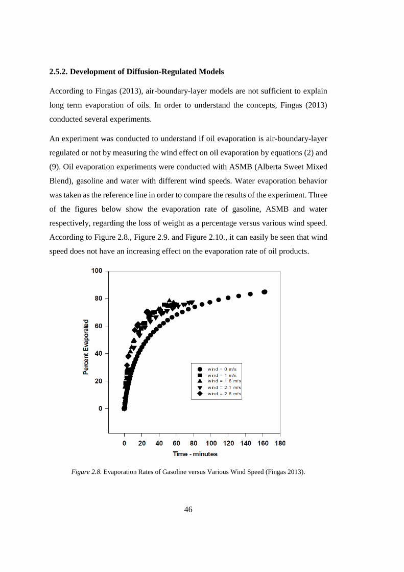
46

2.5.2. Development of Diffusion-Regulated Models

According to Fingas (2013), air-boundary-layer models are not sufficient to explain

long term evaporation of oils. In order to understand the concepts, Fingas (2013)

conducted several experiments.

An experiment was conducted to understand if oil evaporation is air-boundary-layer

regulated or not by measuring the wind effect on oil evaporation by equations (2) and

(9). Oil evaporation experiments were conducted with ASMB (Alberta Sweet Mixed

Blend), gasoline and water with different wind speeds. Water evaporation behavior

was taken as the reference line in order to compare the results of the experiment. Three

of the figures below show the evaporation rate of gasoline, ASMB and water

respectively, regarding the loss of weight as a percentage versus various wind speed.

According to Figure 2.8., Figure 2.9. and Figure 2.10., it can easily be seen that wind

speed does not have an increasing effect on the evaporation rate of oil products.

Figure 2.8. Evaporation Rates of Gasoline versus Various Wind Speed (Fingas 2013).

47

Figure 2.9. Evaporation Rates of ASMB versus Various Wind Speed (Fingas 2013).

There is only very little change in the evaporation rate from the 0 m/s wind speed to

other wind speed levels. According to Fingas (2013), this can be explained by the

stirring effect of wind but not in terms of air-boundary layer interaction.

Figure 2.10. Evaporation Rates of Water versus Various Wind Speed (Fingas 2013).

48

On the other hand, it can be seen from the Figure 2.10. that there are dramatic changes

in the evaporation rate of water as wind speed increases. According to Fingas (2013),

it can be explained by the air-boundary-layer regulation evaporation model as it is

mentioned before.

Figure 2.11. Wind Velocity versus Evaporation Rates (Fingas, 2013)

Figure 2.11 is obtained by correlation of data from the experiments. It can be seen

from the lines that there is no correlation between wind speed and oil evaporation

rates. On the other hand, there is a strong correlation between water evaporation and

wind speed. As wind speed increases the evaporation rate of water also increases.

49

As a result of the experiment, it can be seen that the air-boundary-regulation model

does not apply for the evaporation of oil products. However, the stirring effect of wind

for evaporation at the beginning level should not be ignored.

Another important parameter for evaporation is the saturation concentration of oils.

Saturation concentration is the maximum concentration of a liquid that can be soluble

in the air. Table 2.10 shows the saturation concentration of different kinds of oil

products and water. From the table, it is shown that water has a lower saturation

concentration compared to oil products. According to Fingas (2013), this is due to the

fact that oil products have not significant boundary layer limitations.

Table 2.10. Saturation Concentration of Water and Hydrocarbons (Fingas, 2013)

Substance Saturation Concentration

in g/m3 at 25 °C

water 20

n-pentane 1689

hexane 564

cyclohexane 357

benzene 319

n-heptane 196

methylcyclohexane 192

toluene 110

ethylbenzene 40

p-xylene 38

m-xylene 35

o-xylene 29

According to Fingas (2013), there is an important difficulty in modelling of oil

evaporation since every oil product has a different evaporation equation even in

similar conditions. Therefore, it is important to have formerly obtained data to

calculate the evaporation rate of oils. Fingas (2013) says that distillation data is used

to characterize oils and it can be used to calculate the evaporation rate.

50

Oils and diesel fuels have different evaporation equations. Oils have evaporation rates

as a logarithm with time. On the other hand, diesel fuels, like jet fuel which contains

kerosene, have evaporation rate as a square root of time. According to Fingas (2013),

the reason for this situation is that diesel oils contain only fewer number of compounds

which have similar evaporation rates.

The data obtained from experiments at 15 °C were applied to temperature equations.

So, the temperature equations were modified to give:

% 𝐸𝑣𝑎𝑝𝑜𝑟𝑎𝑡𝑖𝑜𝑛 = [𝐵 + 0.045(𝑇 − 15)] ln(𝑡) (37)

In equation (37), B represents the equation factor at 15 °C, T symbolizes temperature

in degrees Celsius and t signifies time as minute.

Fingas (1996) correlated distillation data by experiments so that evaporation rates of

oils are found. It was seen that 180 °C is the optimum temperature for the correlation

of distillation data to evaporation rates. Percentage evaporated at 180 °C was used to

formulate the relationship between distillation and evaporation.

For oils which have a logarithm with time the equation yields as:

𝑃𝑒𝑟𝑐𝑒𝑛𝑡𝑎𝑔𝑒 𝑒𝑣𝑎𝑝𝑜𝑟𝑎𝑡𝑒𝑑 = 0.165(%𝐷) ln(𝑡) (38)

And for diesel-like oils which have square root equation the equation yields as:

𝑃𝑒𝑟𝑐𝑒𝑛𝑡𝑎𝑔𝑒 𝑒𝑣𝑎𝑝𝑜𝑟𝑎𝑡𝑒𝑑 = 0.0254(%𝐷)√𝑡 (39)

where %D is percentage distilled by weight at 180 °C and t is the time in minutes.

Fingas (1996) combined the equations with the equations which were obtained before

so that equations derived to as below:

For oils which have a logarithm with time:

𝑃𝑒𝑟𝑐𝑒𝑛𝑡𝑎𝑔𝑒 𝑒𝑣𝑎𝑝𝑜𝑟𝑎𝑡𝑒𝑑 = [0.165(%𝐷) + 0.045(𝑇 − 15)] ln(𝑡) (40)

And for diesel-like oils which have a square root equation:

51

𝑃𝑒𝑟𝑐𝑒𝑛𝑡𝑎𝑔𝑒 𝑒𝑣𝑎𝑝𝑜𝑟𝑎𝑡𝑒𝑑 = [0.0254(%𝐷) + 0.01(𝑇 − 15)]√𝑡 (41)

where %D is percentage distilled by weight at 180 °C, T is temperature in degrees

Celsius and t is the time in minutes (Fingas, 1996).

Fingas (2013) says that thicker oil spills, more than 2 mm, evaporates much more

slowly compared to thinner spills since they have diffusion regulated evaporation

regulation. Oil compounds have to diffuse longer distances to evaporate in thicker

spills. Additionally, it is totally different from the air-boundary-layer model.

Some experiments were conducted in order to see thickness effect on evaporation with

light crude oil and ASMB. Fingas (2013) says that the most fitting equation can be

obtained by a square root function for the thickness effect correction factor. The

equation is as below:

𝐶𝑜𝑟𝑟𝑒𝑐𝑡𝑒𝑑 𝑒𝑞𝑢𝑎𝑡𝑖𝑜𝑛 𝑓𝑎𝑐𝑡𝑜𝑟 = 𝑒𝑞𝑢𝑎𝑡𝑖𝑜𝑛 𝑓𝑎𝑐𝑡𝑜𝑟 + 1 − 0.78 × √𝑡 (42)

where the corrected equation factor is a factor for oil thickness and t is the thickness

of oil product in millimeter. Fingas (2013) also states that the equation (42) is valid

for evaporation of oil spills with a thickness of more than 1.5 mm.

Fingas (2013) says that there is another important factor called bottle effect that has

an impact on evaporation rates of oils. The evaporation rate is higher when oil is

covered such as in a bottle than it is fully open. It can be explained by impermanent

or partly air-boundary-layer regulated evaporation behavior of oil in the bottle. The

bottle effect ends when the evaporation rate of oil product becomes low compared to

the evaporation rate of oil vapor which evaporates from the bottle mouth.

According to Fingas (2013), it can be seen from the experiments that wind has a slight

effect on the evaporation of oil with respect to the condition with no wind at all. This

is the result of the stirring effect of wind which results in an increased diffusion rate

of oil. However, the same effect does not apply to the evaporation rate of oil as the

velocity of wind increases. As a result, it can only be observed in zero wind conditions.

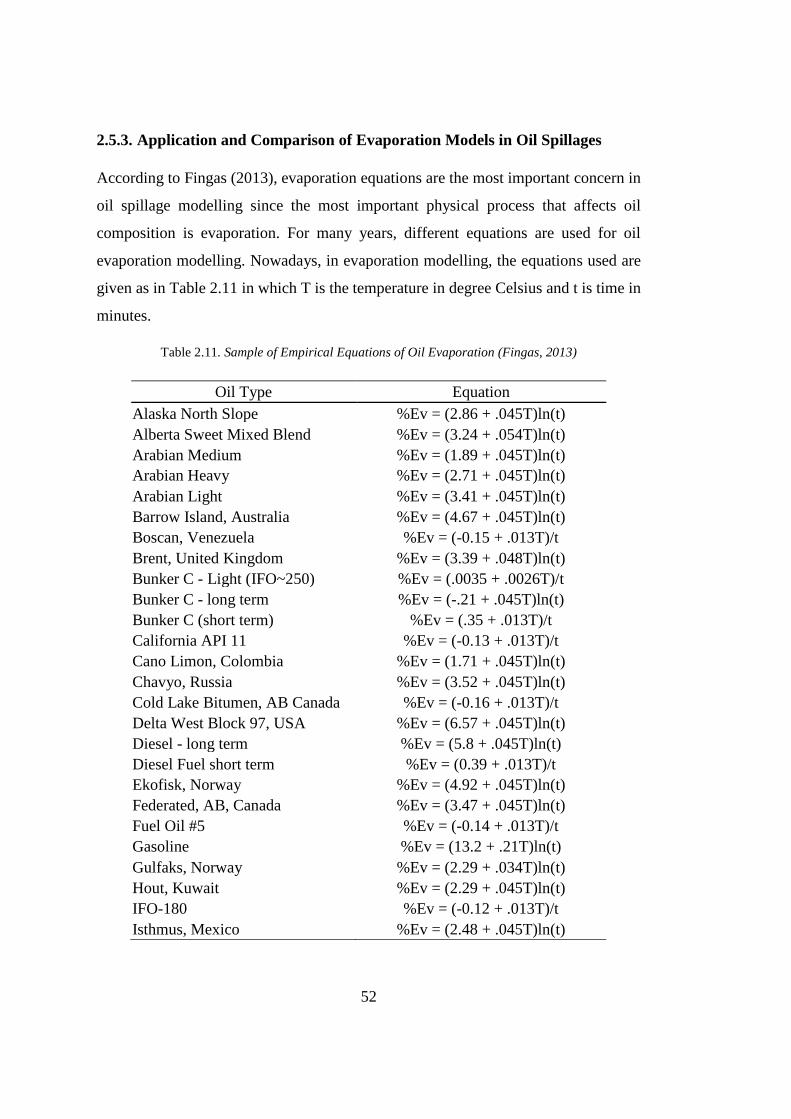
52

2.5.3. Application and Comparison of Evaporation Models in Oil Spillages

According to Fingas (2013), evaporation equations are the most important concern in

oil spillage modelling since the most important physical process that affects oil

composition is evaporation. For many years, different equations are used for oil

evaporation modelling. Nowadays, in evaporation modelling, the equations used are

given as in Table 2.11 in which T is the temperature in degree Celsius and t is time in

minutes.

Table 2.11. Sample of Empirical Equations of Oil Evaporation (Fingas, 2013)

Oil Type Equation

Alaska North Slope %Ev = (2.86 + .045T)ln(t)

Alberta Sweet Mixed Blend %Ev = (3.24 + .054T)ln(t)

Arabian Medium %Ev = (1.89 + .045T)ln(t)

Arabian Heavy %Ev = (2.71 + .045T)ln(t)

Arabian Light %Ev = (3.41 + .045T)ln(t)

Barrow Island, Australia %Ev = (4.67 + .045T)ln(t)

Boscan, Venezuela %Ev = (-0.15 + .013T)/t

Brent, United Kingdom %Ev = (3.39 + .048T)ln(t)

Bunker C - Light (IFO~250) %Ev = (.0035 + .0026T)/t

Bunker C - long term %Ev = (-.21 + .045T)ln(t)

Bunker C (short term) %Ev = (.35 + .013T)/t

California API 11 %Ev = (-0.13 + .013T)/t

Cano Limon, Colombia %Ev = (1.71 + .045T)ln(t)

Chavyo, Russia %Ev = (3.52 + .045T)ln(t)

Cold Lake Bitumen, AB Canada %Ev = (-0.16 + .013T)/t

Delta West Block 97, USA %Ev = (6.57 + .045T)ln(t)

Diesel - long term %Ev = (5.8 + .045T)ln(t)

Diesel Fuel short term %Ev = (0.39 + .013T)/t

Ekofisk, Norway %Ev = (4.92 + .045T)ln(t)

Federated, AB, Canada %Ev = (3.47 + .045T)ln(t)

Fuel Oil #5 %Ev = (-0.14 + .013T)/t

Gasoline %Ev = (13.2 + .21T)ln(t)

Gulfaks, Norway %Ev = (2.29 + .034T)ln(t)

Hout, Kuwait %Ev = (2.29 + .045T)ln(t)

IFO-180 %Ev = (-0.12 + .013T)/t

Isthmus, Mexico %Ev = (2.48 + .045T)ln(t)

53

Table 2.11. Sample of Empirical Equations of Oil Evaporation (Cont’ed) (Fingas, 2013)

Oil Type Equation

Jet A1 %Ev = (.59 + .013T)/t

Komineft, Russian %Ev = (2.73 + .045T)ln(t)

Lago, Angola %Ev = (1.13 + .045T)ln(t)

Lago Treco, Venezuela %Ev = (1.12 + .045T)ln(t)

Maya, Mexico %Ev = (1.38 + .045T)ln(t)

Sahara Blend, Algeria %Ev = (0.001 + .013T)/t

Sakalin, Russia %Ev = (4.16 + .045T)ln(t)

Scotia Light %Ev = (6.87 + .045T)ln(t)

South Louisiana %Ev = (2.39 + .045T)ln(t)

Statfjord, Norway %Ev = (2.67 + .06T)ln(t)

Taching, China %Ev = (-0.11 + .013T)/t

Troll, Norway %Ev = (2.26 + .045T)ln(t)

West Texas Intermediate %Ev = (2.77 + .045T)ln(t)

West Texas Sour %Ev = (2.57 + .045T)ln(t)

Researches on air-boundary-layer evaporation modelling of oil spills result in the

wrong conclusion with respect to empirical values. In Figure 2.12, it can be easily seen

that evaporation modeling of diesel product values of the air-boundary-layer model

and experimental results are very close to each other in the case of no wind. However,

diesel evaporation data obtained with various wind speeds result in big differences as

much as 100% in a longer period of time such as 200 hours.

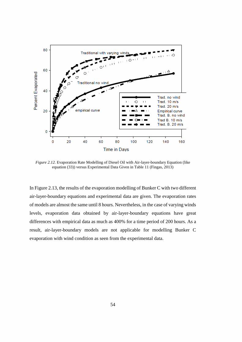
54

Figure 2.12. Evaporation Rate Modelling of Diesel Oil with Air-layer-boundary Equation (like

equation (33)) versus Experimental Data Given in Table 11 (Fingas, 2013)

In Figure 2.13, the results of the evaporation modelling of Bunker C with two different

air-layer-boundary equations and experimental data are given. The evaporation rates

of models are almost the same until 8 hours. Nevertheless, in the case of varying winds

levels, evaporation data obtained by air-layer-boundary equations have great

differences with empirical data as much as 400% for a time period of 200 hours. As a

result, air-layer-boundary models are not applicable for modelling Bunker C

evaporation with wind condition as seen from the experimental data.

55

Figure 2.13. Evaporation Rate Modelling of Bunker C with Air-layer-boundary Equation (like

equation (33)) versus Experimental Data Given in Table 11 (Fingas, 2013)

Thus, Fingas (2013) concludes that air-layer-boundary modelling of oil results in three

main errors. Firstly and most importantly, with air-layer-boundary modelling, accurate

long term evaporation rates cannot be obtained. Secondly, results in the case of

different wind levels are impossible in reality. Finally, air-layer-boundary models do

not give accurate evaporation rate curves for diesel oils. Fingas (2013) says that in

order to obtain realistic results with air-layer-boundary equations, many researchers

set maximum allowable evaporation value for long term evaporation modelling. For

example, in Alberta of Pembina, an oil spill was analyzed by taking samples after 30

years and the evaporation rate was found to be 58%. In Figure 2.14, actual data,

experimental prediction and air-layer-boundary modelling results are given. As it can

be seen from the figure, actual analysis and empirical data are similar. However, the

prediction made by air-layer-boundary modelling results in unrealistic values.

56

Figure 2.14. Evaporation Rate Modelling of Pembina Crude Oil with Air-layer-boundary Equation

(like equation (33)) versus Real Data and Experimental Curve (Fingas, 2013)

In conclusion, the evaporation of oil cannot be modeled as an air-boundary-layer

regulation. There are many experiments that show air-boundary-layer regulated

modeling does not result in accurate evaporation rates. Hence, simpler evaporation

modeling equations can be enough to describe the evaporation of oil products.

Additionally, wind speed, turbulence of wind, area and scale size do not have major

importance in oil evaporation modelling. In the oil evaporation process, the most

important factors that should be taken into consideration are time and temperature.

The application of air-boundary-layer equations to predict oil evaporation for spillage

gives unrealistic evaporation rates. According to Fingas (2013), there are three main

reasons for inaccurate modeling results. First, air-boundary-layer equations do not

provide accurate evaporation values for a long period of time. Second, the wind effect

57

causes the air-layer-boundary model to be in unreal rates. Third, air-boundary-layer

models are not suitable for predict evaporation curves of oils like diesel.

Fingas (2013) states that diffusion-regulated equations are as accurate as empirical

evaporation equations for oil products. Diffusion-regulated equations are used in the

form given in equation (38). Fingas (2013) also says that diesel-like oils have the

evaporation curve which follows the square root curve as given in equation (39).

According to Fingas (2013), in evaporation modeling, the best results can be achieved

by using experimental equations as given in Table 2.11. If empirical equations are not

present, distillation data can be used as given in equations (40) and (41).

According to Mackay and Wesenbeeck (2014), the evaporation rate is a concern for

chemical exposure prediction in chemical spills. Evaporation rate and vapor pressure

of substance have a relation. The relationship between evaporation rate and vapor

pressure is established by Mackay and Wesenbeeck for several substances.

Evaporation rate can be affected by numerous factors such as solar radiation, wind

speed and humidity. However, these factors are not included in the determined

formulation for the evaporation rate.

According to ideal gas law, on a solid and non-absorbing surface, a pure liquid

substance has a saturated vapor concentration as indicated in equation (43) or (44).

𝐶𝑠 = 𝑃 𝑅𝑇⁄ (43)

𝐶𝑠 = 𝑃𝑀 𝑅𝑇⁄ (44)

In equation (43) and (44), P is vapor pressure in Pa, M is molar weight in kg/mol, R

is gas constant as 8.314 Pa m3 /mol K and T is absolute temperature in K. Therefore,

𝐶𝑠 is in mol/m3 in equation (43) and kg/m3 in equation (44).

Evaporation rate can be thought as the result of saturated vapor concentration and

mass transfer constant, k as m/s which is the speed of transfer of saturated air from the

liquid surface. Similar to Fick’s law, diffusivity is D in m2s-1 and diffusion path length

58

is Y in m, then k is equal to DY-1. Thus, the evaporation rate is defined as molar flux

and mass flux in equation (45) and (46) as:

𝐸 = 𝑃𝑘 𝑅𝑇⁄ (45)

𝐸 = 𝑃𝑀𝑘 𝑅𝑇⁄ (46)

In equation (45), evaporation rate, E is in mol/m2s and in equation (46), E is in kg/m2s.

Mackay and Wesenbeeck (2014) says that there is a correlation between E and P but

not PM. The slope of the plot of log E versus log P is less than 1. This can be expressed

by the absence of M in the correlation. Chemicals with higher molecular mass have

lower volatility. If correlation is changed to evaporation rate in molar flux versus

pressure than evaporation rate decreases and slope increases. E is modified to mol/m2s

and the slope of the plot is obtained closer to 1. Therefore, there is no need for a

logarithmic correlation between E and P. The relationship between E and P can be

expressed as simple and one parameter formula. Correlation between molar

evaporation rate, E and pressure, P is given in the Figure 2.15.

Figure 2.15. Plot of Molar Evaporation Rate, E vs. Pressure, P

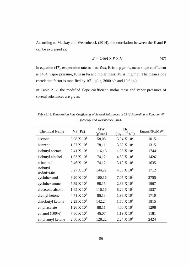
59

According to Mackay and Wesenbeeck (2014), the correlation between the E and P

can be expressed as:

𝐸 = 1464 × 𝑃 × 𝑀 (47)

In equation (47), evaporation rate as mass flux, E, is in µg/m2s, mean slope coefficient

is 1464, vapor pressure, P, is in Pa and molar mass, M, is in g/mol. The mean slope

correlation factor is modified by 109 µg/kg, 3600 s/h and 10-3 kg/g.

In Table 2.12, the modified slope coefficient, molar mass and vapor pressures of

several substances are given.

Table 2.12. Evaporation Rate Coefficients of Several Substances at 25 °C According to Equation 47

(Mackay and Wesenbeeck, 2014)

Chemical Name VP (Pa) MW

(g/mol)

ER

(mg m−2 s−1) Emass/(PxMW)

acetone 3.08 X 104 58,08 5.04 X 102 1015

benzene 1.27 X 104 78,11 3.62 X 102 1315

isobutyl acetate 2.41 X 103 116,16 1.36 X 102 1744

isobutyl alcohol 1.53 X 103 74,12 4.50 X 101 1426

n-butanol 9.46 X 102 74,12 3.19 X 101 1635

isobutyl

isobutyrate 6.27 X 102 144,22 4.30 X 101 1712

cyclohexanol 9.20 X 101 100,16 7.05 X 100 2755

cyclohexanone 5.39 X 102 98,15 2.89 X 101 1967

diacetone alcohol 1.65 X 102 116,16 8.20 X 100 1537

diethyl ketone 4.71 X 103 86,13 1.93 X 102 1710

diisobutyl ketone 2.23 X 102 142,24 1.60 X 101 1815

ethyl acetate 1.26 X 104 88,11 4.00 X 102 1298

ethanol (100%) 7.86 X 103 46,07 1.19 X 102 1181

ethyl amyl ketone 2.60 X 102 128,22 2.24 X 101 2424

60

Table 2.12. Evaporation Rate Coefficients of Several Substances at 25 °C According to Equation 47

(Cont’ed) (Mackay and Wesenbeeck, 2014)

Chemical Name VP (Pa) MW

(g/mol)

ER

(mg m−2 s−1) Emass/(PxMW)

ethylbenzene 1.28 X 103 106,17 6.82 X 101 1812

ethyl lactate 5.00 X 102 118,13 1.80 X 101 1096

n-hexane 2.02 X 104 86,18 5.87 X 102 1215

isophorone 5.73 X 101 138,21 2.17 X 100 988

mesityl oxide 1.46 X 103 98,15 7.23 X 101 1820

methanol 1.70 X 104 32,04 1.37 X 102 905

nitroethane 2.80 X 103 75,07 1.21 X 102 2078

nitromethane 4.77 X 103 61,04 1.57 X 102 1936

1-nitropropane 1.37 X 103 89,09 7.62 X 101 2247

n-octane 1.85 X 103 114,23 1.17 X 102 1993

n-propyl acetate 4.49 X 103 102,13 1.92 X 102 1504

isopropyl alcohol 5.69 X 103 60,1 7.56 X 101 796

n-propyl alcohol 2.83 X 103 60,1 6.00 X 101 1271

tetrahydrofuran 2.17 X 104 72,11 4.68 X 102 1078

toluene 3.80 X 103 92,14 1.82 X 102 1873

p-xylene 1.17 X 103 106,17 7.00 X 101 2024

dodecane 1.23 X 101 170,34 2.75 X 10−1 474

n-octanol 1.73 X 101 130,23 3.75 X 10−1 599

tridiphane 2.93 X 10−2 320,43 1.98 X 10−3 759

trifluralin 1.47 X 10−2 335,29 4.41 X 10−4 322

pendimethalin 4.00 X 10−3 281,31 2.89 X 10−4 924

2,4-D 2.67 X 10−3 221,04 1.86 X 10−4 1135

diazinon 1.49 X 10−3 304,35 2.52 X 10−4 2004

toxaphene 5.33 X 10−4 413,82 5.53 X 10−5 902

dieldrin 6.59 X 10−4 380,91 4.78 X 10−5 685

61

According to Table 2.12, dodecane has an evaporation rate equation as:

𝐸 = 474 × 𝑃 × 𝑀 (48)

In equation (48), E is the evaporation rate in µg/m2s, vapor pressure, P, is in Pa and

molar weight is in g/mol.

The purposed methodology offers linear regression with one parameter. In practice,

the evaporation rate can be affected by several environmental factors such as wind

speed, temperature and radiation. If environmental factors are taken into account, the

correlation becomes more accurate but more complex to handle. However, simple

approaches can be used for checking data obtained from the field. Unfortunately, this

approach can be applied to estimate the evaporation of pure substances.

2.6. Dispersion of Air Pollutants

Air pollutants do not stay at their discharge point. Atmospheric motions and physical

conditions move particles emitted in the air. Therefore, it is important to understand

the mechanism which affects the dispersion process of airborne particles (Spellman &

Stoudt, 2013). The concentration of a contaminant at a specific location is

correspondent to several factors such as emission rates, distance from the source and

meteorological conditions (Abdel-Rahman, 2008).

2.6.1. Weather

Atmospheric conditions significantly affect pollutant concentration, in a positive or

negative manner, particularly on the local scale (Spellman & Stoudt, 2013). Variation

of atmospheric factors can cause the concentration of a substance in the air to be

affected by 10 times even in a case of steady wind flow. Obviously, meteorological

factors are significant for accurate modeling of air pollution dispersion. On the other

hand, mainly microscale atmospheric conditions are concern with air dispersion

62

modelling. Atmospheric conditions on the larger scale have also an effect on

dispersion, however, their effect is only significant for pollution with a longer period

of time than 1 hour (De Visscher, 2014).

Meteorological conditions affect substance concentration in the air mechanically and

chemically. Weather conditions can ease airborne substances to precipitate

mechanically which causes a decrease in concentration. Particle concentration in the

air is diluted by wind which brings clean air. Air and the pollutant contained by air

rise as the sun heat up the upper atmosphere.

Atmospheric factors such as wind and turbulence can mix two different air

contaminants which give a chemical reaction and form another hazardous substance

(Spellman & Stoudt, 2013).

2.6.2. Turbulence

Turbulence in the air is a significant factor which affects air dispersion of

contaminants. Since turbulence provides fresh air to the contaminated air mixture, the

concentration of pollutants decreases. Turbulence is caused by wind speed which is a

result of temperature difference in the atmosphere proportional to elevation.

Therefore, turbulence is related to stability which is correspondent to vertical

temperature distribution in the atmosphere (Spellman & Stoudt, 2013). Stability

means the tendency or resistance of air to move vertically which is crucial for pollution

dispersion (Nesaratnam and Taherzadeh, 2014). In other words, if air resists vertical

movement it can be regarded as stable, if air develops vertical motion then it can be

assumed to be unstable (Boubel et al., 1994).

Pasquill (1961) categorized atmospheric stability classes into six different groups.

Pasquill’s stability classes are shown in Table 2.13. Sutherland et al. (1986) states that

stability class can also be decided qualitatively from atmospheric conditions by

practical skills.

63

Table 2.13. Pasquill’s Atmospheric Stability Classes

Pasquill

stability class Condition

A extremely unstable

B moderately unstable

C slightly unstable

D neutral

E slightly stable

F moderately stable

Pasquill (1961) also proposed key characteristics for deciding the stability category of

the atmospheric conditions. Table 2.14 shows the key characteristics of the stability

categories.

Table 2.14. Key to Stability Categories

Surface

wind

speed (at

10 m)

m/sec

Insolation Night

Strong Moderate Slight

Thinly

overcast or

≥4/8 low

cloud

≤3/8

cloud

<2 A A-B B - -

2-3 A-B B C E F

3-5 B B-C C D E

5-6 C C-D D D D

>6 C D D D E

Atmospheric stability classes are used to define the dispersion rate of airborne

contaminants (Chapman, 2017). Spellman & Stoudt (2013) says that stable

meteorological conditions results in low wind speeds accordingly lower level of

turbulence. Therefore, low turbulence has an adversary effect on the dispersion of

contaminants (Spellman & Stoudt, 2013). On the contrary, if rising pollutants do not

reach stable atmospheric conditions then they are diluted by turbulence which ease the

dispersion of contaminants (Hanna et al., 1982).

64

2.6.3. Topography

Topography has an important effect on airflow patterns and dispersion of pollutants

from point and area sources (Spellman & Stoudt, 2013). Complex topographical

structures in a region have a powerful influence on wind patterns which cause

alteration in the stability of atmospheric conditions affecting contaminant dispersal

(Valdenebro et al., 2014).

According to Nesaratnam and Taherzadeh (2014), buildings cause turbulence which

has an effect on pollutant dispersion. Wind is divided into two parts in the front part

of the building and as a result, the distributed wind covers the structure twice its height

by upwards and five to ten times its height by downwind direction. Figure 2.16 shows

the effect of a building to the flow of wind.

Figure 2.16. The Effect of a Building to the Flow of Wind

Temperature change, pressure change and friction which is related to surface

roughness, affects wind speed (Godish, 2004). The effect of urban, suburbs and rural

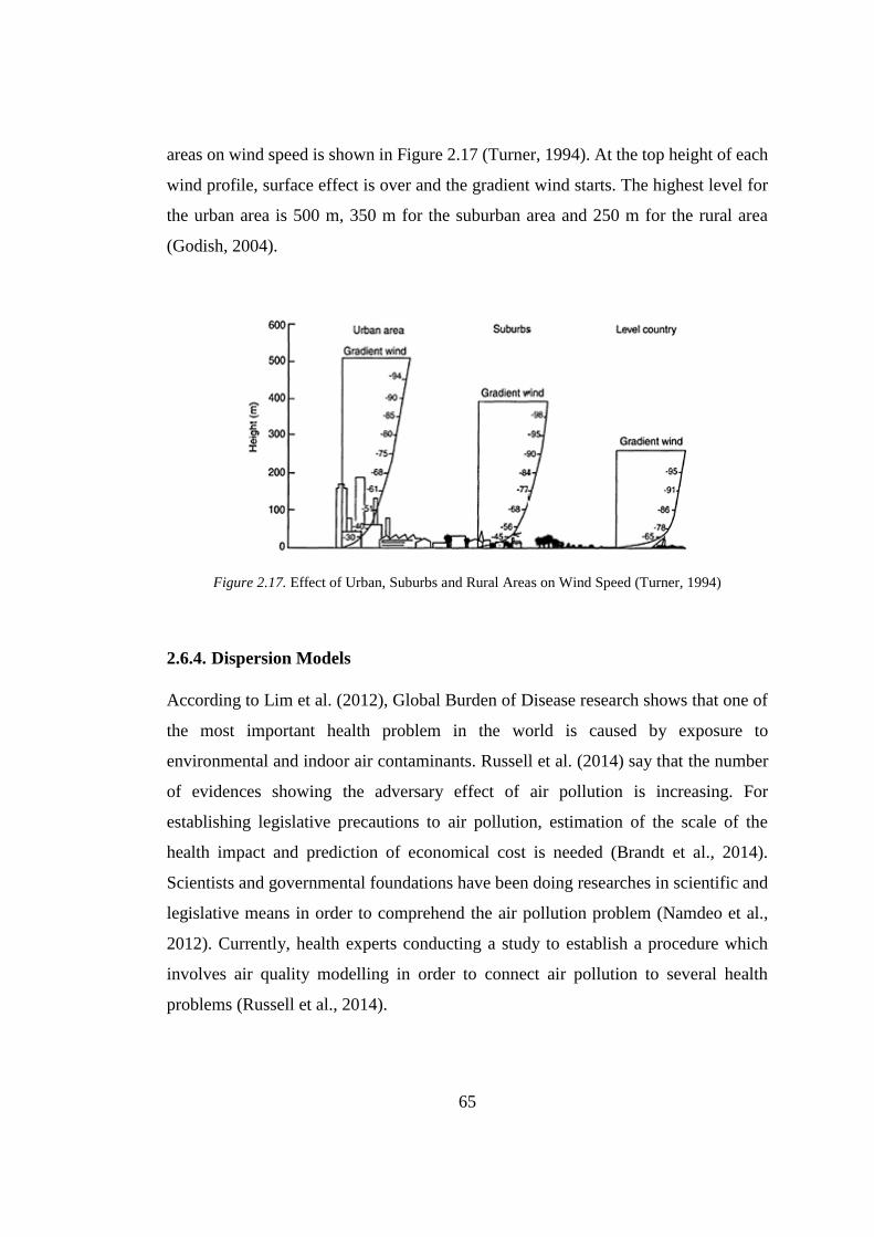
65

areas on wind speed is shown in Figure 2.17 (Turner, 1994). At the top height of each

wind profile, surface effect is over and the gradient wind starts. The highest level for

the urban area is 500 m, 350 m for the suburban area and 250 m for the rural area

(Godish, 2004).

Figure 2.17. Effect of Urban, Suburbs and Rural Areas on Wind Speed (Turner, 1994)

2.6.4. Dispersion Models

According to Lim et al. (2012), Global Burden of Disease research shows that one of

the most important health problem in the world is caused by exposure to

environmental and indoor air contaminants. Russell et al. (2014) say that the number

of evidences showing the adversary effect of air pollution is increasing. For

establishing legislative precautions to air pollution, estimation of the scale of the

health impact and prediction of economical cost is needed (Brandt et al., 2014).

Scientists and governmental foundations have been doing researches in scientific and

legislative means in order to comprehend the air pollution problem (Namdeo et al.,

2012). Currently, health experts conducting a study to establish a procedure which

involves air quality modelling in order to connect air pollution to several health

problems (Russell et al., 2014).

66

Air dispersion modeling continues to be developed for over decades (Sriram et al.

2006). There are many different models for air dispersion varying from simple

Gaussian plume models to complex computational fluid dynamics models (De

Visscher, 2014). Air dispersion modelling provides an estimation of the concentration

of pollutants at a specific distance from the pollution source (Spellman & Stoudt,

2013). De Visscher (2014) claims that generally basic air dispersion models have more

accuracy in pollutant concentration prediction than complex models. Though, every

dispersion model has a handicap and high accuracy is not certain. In general, high

accuracy can be reached by correct model selection regarding model requirements and

circumstances. Singh (2018) says that there are five different models available for air

pollutant dispersion:

1. Box Model

2. Gaussian Model

3. Lagrangian Model

4. Eulerian Model

5. Dense gas model

According to Artana et al., (2014), some scientists also examine hybrid models which

are a combination of different dispersion models.

Currently, the most widely used model of air dispersion estimation is Gaussian Plume

Model and its modified versions (Sriram et al. 2006). According to Spellman & Stoudt

(2013), during air dispersion modelling four-step procedure is recommended to

follow:

1. Determine the rate, duration and location of the emission

2. Decide the best suitable model to conduct dispersion modelling study

3. Calculate the concentration of pollutant at the specific location

4. Determine possible outcomes according to the modelling process.

67

2.6.5. Box Model

Markiewicz (2006) claims that the box model is the simplest model among all other

dispersion models. According to the box model, the atmosphere is thought to be

separated into equal size of numerous boxes (Indra et al., 2004). It is assumed that

emission from the source is constant over a distance ∆x. It is also assumed that the

concentration of the pollutant is constant in the box due to uniform mixing. In the box,

the wind velocity is taken as a constant value. In the box model, mixing height is

tought to be increasing with respect to time. Thus, the box model equation can be

expressed as (Hanna et al., 1982):

∆𝑥 𝑧𝑖 𝜕𝐶

𝜕𝑡= ∆𝑥 𝑄 + 𝑢 𝑧𝑖(𝐶𝑏 − 𝐶) + ∆𝑥

𝜕𝑧𝑖

𝜕𝑡 (𝐶𝑎 − 𝐶) (49)

Change in the C

with time = source +

change due

to horizontal

advection

+

change due to mixing

layer growth and

vertical advection

In equation (49), 𝑄 represents the emission rate in mass per unit time per unit area, 𝐶𝑏

and 𝐶𝑎 symbolize concentrations upwind and above the mixing height respectively. In

steady-state conditions, 𝐶𝑏, 𝜕𝐶

𝜕𝑡 and

𝜕𝑧𝑖

𝜕𝑡 is equal to 0 hence, the equation (49) yields to:

𝐶 =∆𝑥 𝑄

𝑧𝑖 𝑢 (50)

Box model diagram can be seen in Figure 2.18.

68

Figure 2.18. Box Model Diagram (Hanna et al., 1982)

Hanna et al. (1982) state that generally governmental foundations use the box model

for detecting some specific substances to take into consideration solely among a group

of hazardous chemicals. In general, the box model is regarded as a fundamental

approach for dispersion modelling and good results have been obtained. On the other

hand, Spellman & Stoudt (2013) claim that since assumptions in the box model are

very simple, the accuracy of the model is limited in air dispersion estimation.

2.6.6. Gaussian Model

The first and most widely used air dispersion model is Gaussian model. It is assumed

that the dispersion of pollutants has a Gaussian distribution model. In general, the

Gaussian model is applied to steady-state air pollutant emission from the sources at

ground-level or at a specific height (Spellman & Stoudt, 2013). The Gaussian model

can be used for calculations to determine the concentration of the pollutant emitted

from a source (Beychok, 2005). Empirically, the model can be defined drawn as

69

standard deviation of concentration in y and z-axis correspondent to atmospheric

stability classes and downwind distance from the emission point (Singh, 2018).

In case of modeling emissions from ground level area sources, it can be assumed that

there are many point sources which have individual emissions. All emissions from

each point source in the area can be combined by assuming that there is an initial

horizontal standard deviation, σy0. A virtual distance, xy, can be determined to give

horizontal standard deviation, σy0. This value is used to determine σy according to

atmospheric stability class. After that, model for point source can be used to determine

σy as a function of x + xy. According to this theory, area source can be thought as a

crosswind line source with a Gaussian distribution. The initial horizontal standard

deviation, σy0, for an area source can be calculated by σy0 = s/4.3, where s is the length

of the area source (Turner, 1994).

According to Indra et al. (2004), in Gaussian modelling of a plume of a single stack,

the assumptions made are as:

1. Distribution of concentration in the plume is Gaussian in both y and z-axis

2. Wind velocity, u, and wind direction is constant

3. Continuous and constant emission rate of pollutant, Q

4. Dispersion in x-axis is negligible

5. The pollutant does not have a chemical reaction

6. Steady-state and homogeneous transportation of pollutants

7. Topography is negligible

On the other hand, Singh (2018) mentions additional assumptions such as:

1. There is no background pollution

2. Mass is preserved by reflection from the ground

Hence, the Gaussian dispersion model can be expressed as:

70

𝐶 =𝑄

2𝜋𝑢𝜎𝑦𝜎𝑧𝑒𝑥𝑝 (−

𝑦2

2𝜎𝑦2) 𝑒𝑥𝑝 [−

(𝑧−ℎ)2

2𝜎𝑧2 ] (51)

In equation (51), C represents the concentration of the pollutant at a given point, Q

symbolizes the emission rate of the pollutant, u is the wind velocity, 𝜎𝑦 signifies

horizontal dispersion parameter, 𝜎𝑧 is the vertical dispersion parameter, h is the

effective height (De Visscher, 2014).

Figure 2.19 shows the Gaussian dispersion model (Nesaratnam and Taherzadeh,

2014).

Figure 2.19. Gaussian Dispersion Model (Nesaratnam and Taherzadeh, 2014).

According to the assumption of mass is preserved by reflection from the ground, a

reflected source is added to the equation and equation (51) yields (De Visscher, 2014):

71

𝐶 =𝑄

2𝜋𝑢𝜎𝑦𝜎𝑧𝑒𝑥𝑝 (−

𝑦2

2𝜎𝑦2) {𝑒𝑥𝑝 [−

(𝑧−ℎ)2

2𝜎𝑧2 ] + 𝑒𝑥𝑝 [−

(𝑧+ℎ)2

2𝜎𝑧2 ]} (52)

Figure 2.20 shows non-buoyant Gaussian dispersion model from a ground source.

Figure 2.21 demostrates reflected source due to ground reflection.

Figure 2.20. Non-buoyant Gaussian Dispersion from a Ground Source (Pursuer et al., 2016).

Figure 2.21. Reflected source due to ground reflection (Cooper and Alley, 2011)

72

From the equation (52), it can be concluded that (De Visscher, 2014):

1. The pollution concentration is correspondent to the emission rate

2. The pollution concentration has inverse proportion to wind velocity: high

velocity of wind results in low pollutant concentration

3. In the case of the plume rise is affected by emission and wind speed, hence,

the first two conclusions are only approximations.

According to Hanna et al. (1982), it should also be considered what would happen if

wind velocity, u, is measured as zero in the Gaussian model. Hanna et al. (1982) states

that anemometers can give a measurement result as u≈0 near the surface however it

should be suitable to take u as 0.5 m/s since it is not possible for the wind to stop

completely at the surface of the ground.

In general, the main concern is the ground level concentration of pollutant regarding

public health. At ground level, where z=0, the equation is derived to (Nesaratnam and

Taherzadeh, 2014):

𝐶 =𝑄

𝜋𝑢𝜎𝑦𝜎𝑧𝑒𝑥𝑝 (−

𝑦2

2𝜎𝑦2) 𝑒𝑥𝑝 (−

ℎ2

2𝜎𝑧2) (53)

Nesaratnam and Taherzadeh (2014) also state that the maximum concentration of the

pollutant can be observed at the center line of the plume, where y=0, therefore

equation (53) can be written as:

𝐶 =𝑄

𝜋𝑢𝜎𝑦𝜎𝑧𝑒𝑥𝑝 (−

ℎ2

2𝜎𝑧2) (54)

If the emission is at ground level and there is no effective plume rise, h=0, then the

equation is derived to (Godish, 2004):

𝐶 =𝑄

𝜋𝑢𝜎𝑦𝜎𝑧 (55)

73

In the Gaussian dispersion model, in order to determine pollutant concentration at the

desired downwind distance, two stages of calculation should be conducted (Singh,

2018):

1. Effective height should be calculated by adding plume rise at specific

downwind distance from the pollutant source to the height of the source.

2. Pollutant concentration at the desired downwind distance by applying the

Gaussian dispersion model.

2.6.7. Dispersion Parameters

In the Gaussian dispersion model, σy and σz symbolize the standard deviation of the

horizontal and vertical dispersion parameters respectively. Bigger value of dispersion

parameter, σ, results in wider distribution. Accordingly, the plume spreads wider as

the downwind distance from the pollution source increases and dispersion parameters

have bigger values. In other words, dispersion parameters are correspondent to value

of downwind distance, x (Nesaratnam and Taherzadeh, 2014).

Godish (2004) says that the increase in the ratio of dispersion coefficients is

proportional to meteorological parameters, specifically atmospheric stability. In the

atmospheric stability of class A, the amount of increase is maximum for dispersion

coefficients. On the other hand, in the atmospheric stability of class F, the degree of

increase is minimum for dispersion coefficients. Generally, σy is not affected by

inversion conditions, hence, σy has a bigger value than σz. Dispersion coefficients, σy

and σz, can be found from Figure 2.22 and Figure 2.23 respectively.

74

Figure 2.22. Horizontal Dispersion Coefficient, σy , vs. Downwind Distance, x (Godish, 2004).

Figure 2.23. Vertical Dispersion Coefficient, σz , vs. Downwind Distance, x (Godish, 2004).

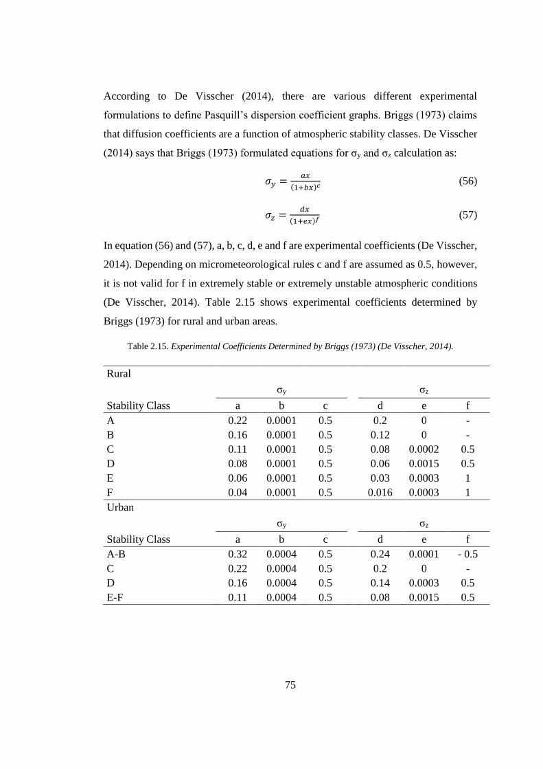
75

According to De Visscher (2014), there are various different experimental

formulations to define Pasquill’s dispersion coefficient graphs. Briggs (1973) claims

that diffusion coefficients are a function of atmospheric stability classes. De Visscher

(2014) says that Briggs (1973) formulated equations for σy and σz calculation as:

𝜎𝑦 =𝑎𝑥

(1+𝑏𝑥)𝑐 (56)

𝜎𝑧 =𝑑𝑥

(1+𝑒𝑥)𝑓 (57)

In equation (56) and (57), a, b, c, d, e and f are experimental coefficients (De Visscher,

2014). Depending on micrometeorological rules c and f are assumed as 0.5, however,

it is not valid for f in extremely stable or extremely unstable atmospheric conditions

(De Visscher, 2014). Table 2.15 shows experimental coefficients determined by

Briggs (1973) for rural and urban areas.

Table 2.15. Experimental Coefficients Determined by Briggs (1973) (De Visscher, 2014).

Rural σy σz

Stability Class a b c d e f

A 0.22 0.0001 0.5 0.2 0 -

B 0.16 0.0001 0.5 0.12 0 -

C 0.11 0.0001 0.5 0.08 0.0002 0.5

D 0.08 0.0001 0.5 0.06 0.0015 0.5

E 0.06 0.0001 0.5 0.03 0.0003 1

F 0.04 0.0001 0.5 0.016 0.0003 1

Urban

σy σz

Stability Class a b c d e f

A-B 0.32 0.0004 0.5 0.24 0.0001 - 0.5

C 0.22 0.0004 0.5 0.2 0 -

D 0.16 0.0004 0.5 0.14 0.0003 0.5

E-F 0.11 0.0004 0.5 0.08 0.0015 0.5

76

In order to have an idea about the accuracy of the Briggs’ equation, dispersion

coefficients graph according to downwind distance for rural terrain is given in

Figure24 (a) and (b) (De Visscher, 2014).

Martin (1976) formulized an equation for σy and σz as:

𝜎𝑦 = 𝑎𝑋𝑏 (58)

𝜎𝑧 = 𝑐𝑋𝑑 + 𝑓 (59)

In equation (58) and (59), a, c, d and f are stability coefficients, b is constant which is

equal to 0.849.

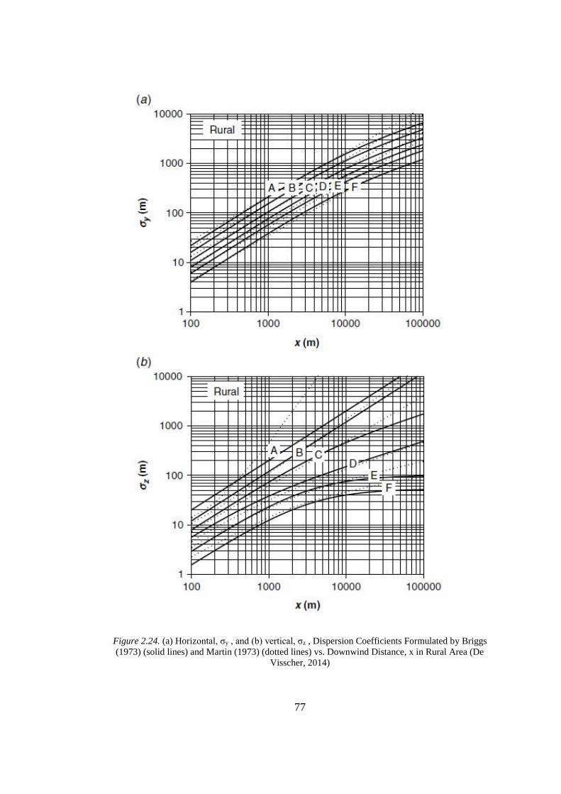
77

Figure 2.24. (a) Horizontal, σy , and (b) vertical, σz , Dispersion Coefficients Formulated by Briggs

(1973) (solid lines) and Martin (1973) (dotted lines) vs. Downwind Distance, x in Rural Area (De

Visscher, 2014)

78

2.6.8. Lagrangian Model

Lagrangian model can be used as another technique for pollutant dispersion

modelling. In the Lagrangian model, particle movement is correspondent to

instantaneous flow (Zannetti,1990). According to Weber (1982), distinct air parcels

are monitored and concentration is calculated for every single parcel in Lagrangian

modelling. The conception of air parcel is frequently used in atmospheric science. An

air parcel can be described as a volume of air which is sufficiently big to contain the

adequate number of molecules to have characteristics such as density, temperature and

contaminant concentration (Lin, 2012). The Lagrangian particle trajectory model

complies with the similar assumptions made by puff dispersion models (Walcek,

2002). Figure 2.25 shows the movement of a particle in the random walk model.

Figure 2.25. Movement of a Particle in the Random Walk Model (Vallero, 2014)

Movement of a particle in the random walk model can be formulated by Lagrangian

approach as:

�⃗� = [𝑥(𝑡), 𝑦(𝑡), 𝑧(𝑡)] (60)

79

The Lagrangian model calculates statistics of the trajectories of particles representing

the entire plume to determine pollutant dispersion (Vallero, 2014). Figure 2.26 shows

Lagrangian Model for a vertical column of boxes.

Figure 2.26. Lagrangian Model for a Vertical Column of Boxes (Zannetti,1990).

In the Lagrangian model, assumptions are similar to puff dispersion models. In puff

model, pollutant is emitted from the source and disperses in the air by constant wind

speed and diffusivities. Additionally, pollutant dispersion is constrained by ground

level, z=0, at the bottom and planetary boundary layer (PBL) at the top in the vertical

dimension. The Lagrangian model describes the concentration of the pollutant in the

center of the puff as:

𝐶(𝑥,𝑦,𝑧) =𝑄

(2𝜋)3 2⁄ 𝜎𝑦𝜎𝑧 𝑒𝑥𝑝 (

−(𝑥−𝑥𝑐)2−(𝑦−𝑦𝑐)2

2𝜎𝑦) [𝑒𝑥𝑝 (

−(𝑧−𝑧𝑐)2

2𝜎𝑧) + 𝑒𝑥𝑝 (

−(𝑧+𝑧𝑐)2

2𝜎𝑧)](61)

In equation (61), 𝑥𝑐 and 𝑦𝑐 is the center of the puff, 𝑧𝑐 puff dispersion height, 𝜎𝑦 and 𝜎𝑧

are horizontal and vertical dispersion coefficients respectively (Singh, 2018).

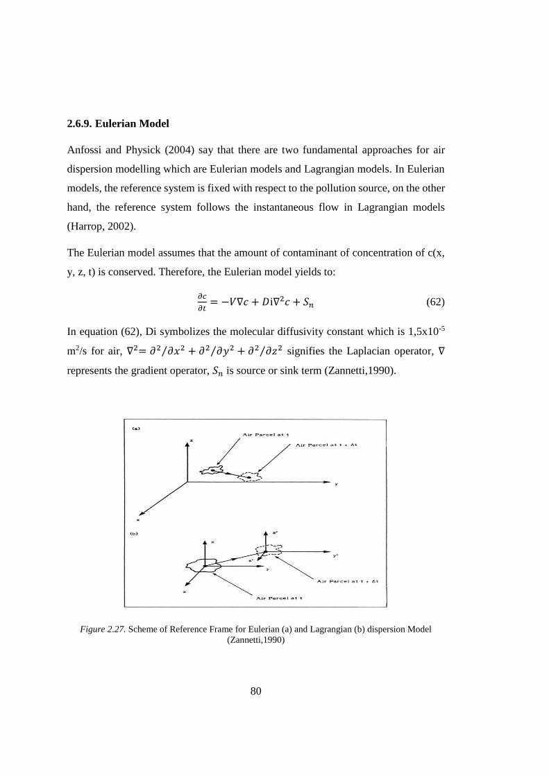
80

2.6.9. Eulerian Model

Anfossi and Physick (2004) say that there are two fundamental approaches for air

dispersion modelling which are Eulerian models and Lagrangian models. In Eulerian

models, the reference system is fixed with respect to the pollution source, on the other

hand, the reference system follows the instantaneous flow in Lagrangian models

(Harrop, 2002).

The Eulerian model assumes that the amount of contaminant of concentration of c(x,

y, z, t) is conserved. Therefore, the Eulerian model yields to:

𝜕𝑐

𝜕𝑡= −𝑉∇𝑐 + 𝐷i∇2𝑐 + 𝑆𝑛 (62)

In equation (62), Di symbolizes the molecular diffusivity constant which is 1,5x10-5

m2/s for air, ∇2= 𝜕2 𝜕𝑥2⁄ + 𝜕2 𝜕𝑦2⁄ + 𝜕2 𝜕𝑧2⁄ signifies the Laplacian operator, ∇

represents the gradient operator, 𝑆𝑛 is source or sink term (Zannetti,1990).

Figure 2.27. Scheme of Reference Frame for Eulerian (a) and Lagrangian (b) dispersion Model

(Zannetti,1990)

81

According to Singh (2018), characteristics of the atmosphere such as temperature,

pressure and concentration of pollutants can be monitored by Eulerian modelling.

Eulerian dispersion model is not accurate at short distances modelling because

turbulent eddies cannot be neglected regarding downwind distance between pollution

source and the receptor. In contrast, the Lagrangian dispersion model is more accurate

for monitoring pollutant concentration on small scales. Eulerian dispersion model has

more accuracy on the regional scale. Additionally, Eulerian dispersion model

calculations need more computer work than Lagrangian models (De Visscher, 2014).

Scheme of reference frame for Eulerian and Lagrangian dispersion model can be seen

in Figure 2.27.

2.6.10. Dense Gas Model

Emission of pollutants will have an impact starting from the pollution source and the

effect of the pollutant will reduce at downwind locations. The biggest adverse effects

can be revealed by toxic or explosive gas emissions. Therefore, gas dispersion

modeling should be conducted in order to forecast pollution effects. In general,

atmospheric effects enhance dispersion and decrease adverse effects caused by

hazardous gas. This phenomenon is valid for buoyant dispersion from elevated

sources. Nevertheless, for dense gases, dispersion is reduced and the effect area is

more considerable at ground level.

There are many gas pollutants, which are denser than air such as chlorine and LPG.

Thus, dense gas modelling is an important issue (Deaves, 1992). Traditional air

dispersion models are not accurate for evaluation of the outcome of gas emissions

which are denser than air (Spicer & Havens, 1989). Dense gases have a tendency to

stay at ground level (Deaves, 1992). As a result, they cause higher safety risks in

operational areas. According to Deaves (1992), obstacles have a more significant

effect on dense gas dispersion than on elevated emission sources.

82

The dense gas dispersion model is a numerical model which can be applied to

atmospheric dispersion of hazardous gases. The dense gas dispersion model is

applicable to non-buoyant, ground level, continuous, sudden, and time-variant

emissions (EPA, 2002). The dense gas dispersion model can be applied to short-term

releases such as 1 hour or shorter time periods and the area of effect can be estimated.

The dense gas dispersion model is beneficial in case of an excessive amount of

hazardous dense gas releases. The frequently applied dense gas dispersion model are

DEGADIS, SLAB and HEGADIS (Singh, 2018).

DEGADIS can be used for modelling aerosol dispersion with predefined

concentration and density ratio. In DEGADIS, the relation between the concentration

and density of aerosol is correspondent to mole fraction, concentration and mixture

density. SLAB model is applicable to evaporating pools and stack releases. SLAB

model is used for the estimation of downwind centerline concentration and pollutant

puff dimensions (Zapert et al., 1991).

83

CHAPTER 3

3. STATEMENT OF PROBLEM

JP-8 is a widely used jet propellant in the aviation sector. In the aerospace industry,

fueling operations have a risk of JP-8 spillage due to breakage or leakage in fueling

stations. JP-8 vapor is hazardous to health in case of human exposure, flammable and

can explode in the presence of various ignition sources such as open flames, sparks

and static electricity. Therefore, it is important to understand the evaporation and

dispersion process of JP-8 as well as the physical and environmental factors affecting

evaporation and dispersion.

By modeling JP-8 evaporation, concentration, percentage and flammability of the air-

vapor mixture can be known at a specific time and distance after the leakage of the

fuel. Dispersion modeling can be used to determine the concentration of flammable

and hazardous vapors in the air at the time given. The physical and environmental

factors such as the amount of spillage, spillage area, wind speed and temperature affect

the dispersion of particles in the air.

The aim of this study is to model evaporation and dispersion of JP-8 spill according

to the environmental and physical factors and to determine the effects of these factors

on possible outcomes. Therefore, evacuation zones can be determined, precautions for

explosion prevention can be clarified and a scientific approach to explosion protection

can be established in the aerospace industry for oil spills.

85

CHAPTER 4

4. METHODOLOGY

4.1. Introduction

In this current study, JP-8 spill scenario is based on a real accident happened during

the fueling operation of an aircraft in the aerospace industry. In modelling, the

environmental and physical conditions are taken into consideration regarding real

accident area circumstances.

For fueling of aircraft in the fueling station, two operators connected fueling pipe to

the aircraft and started fueling operation. Just after starting fueling, two operators left

the fueling station for 30 minutes lunch break. During the fueling operation, due to the

failure in the gasket of the fuel pump’s pipeline, 4,6 tons of JP-8 leaked. Fortunately,

all JP-8 fuel discharged into the secondary containment of the fuel tank. Fueling tank

is next to fueling hangar in open air area. Additionally, JP-8 spill fully filled secondary

containment tank. However, there was no failure alarm in the fueling system and all

operators were at the lunch break for 30 minutes. After the break, the spill alarm was

given and the spillage was cleaned up by the spill response team at the end of 5 hours

of intervention.

In this thesis, after a spillage due to a failure in the fueling system, evaporation and

dispersion of JP-8 under different physical and environmental conditions are

modelled, effects of physical and environmental factors are observed, evacuation

zones and precautions for fire and explosion prevention are defined.

A steady-state model representing the evaporation of the spillage of JP-8 and

atmospheric dispersion of JP-8 vapors has been established. The spill of JP-8 is

estimated as an instantaneously-formed pool of liquid. In order to determine the

concentration of JP-8 vapors downwind of the spillage, two main models are used in

86

the study. Firstly, the evaporation of JP-8 into the atmosphere is modelled.

Atmospheric and chemical properties are used to calculate the vapor formation of JP-

8. The ingredients of JP-8 assumed to be 100% of kerosene. The evaporation rate of

JP-8, calculated through the evaporation model, is regarded as the emission rate for

the atmospheric dispersion model. The JP-8 spill is assumed to be a ground level,

single and constant point source for air dispersion calculation. The concentration of

JP-8 vapors is modelled as a function of downwind distance. The air dispersion model

of JP-8 provides concentration contour plots of JP-8 at an elapsed time, elevation and

distance. The effects of each physical and environmental parameter on JP-8

concentration are modelled and discussed respectively.

4.2. Fueling Operation Area and Fuel Spill Accident Conditions

During the spill accident, physical and environmental factors have an effect on JP-8

evaporation and dispersion. Physical and environmental parameters can be listed as:

Amount of spill

Spillage area

Ambient temperature

Wind speed in the open air

Atmospheric stability class

Land Characteristic

At the time of the spill accident, the values of the physical and environmental factors

affecting dispersion are given in the Table 4.1.

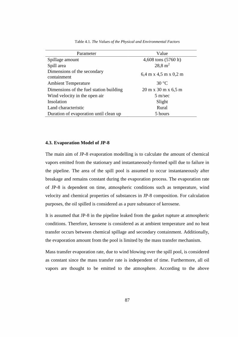
87

Table 4.1. The Values of the Physical and Environmental Factors

Parameter Value

Spillage amount 4,608 tons (5760 lt)

Spill area 28,8 m2

Dimensions of the secondary

containment 6,4 m x 4,5 m x 0,2 m

Ambient Temperature 30 °C

Dimensions of the fuel station building 20 m x 30 m x 6,5 m

Wind velocity in the open air 5 m/sec

Insolation Slight

Land characteristic Rural

Duration of evaporation until clean up 5 hours

4.3. Evaporation Model of JP-8

The main aim of JP-8 evaporation modelling is to calculate the amount of chemical

vapors emitted from the stationary and instantaneously-formed spill due to failure in

the pipeline. The area of the spill pool is assumed to occur instantaneously after

breakage and remains constant during the evaporation process. The evaporation rate

of JP-8 is dependent on time, atmospheric conditions such as temperature, wind

velocity and chemical properties of substances in JP-8 composition. For calculation

purposes, the oil spilled is considered as a pure substance of kerosene.

It is assumed that JP-8 in the pipeline leaked from the gasket rupture at atmospheric

conditions. Therefore, kerosene is considered as at ambient temperature and no heat

transfer occurs between chemical spillage and secondary containment. Additionally,

the evaporation amount from the pool is limited by the mass transfer mechanism.

Mass transfer evaporation rate, due to wind blowing over the spill pool, is considered

as constant since the mass transfer rate is independent of time. Furthermore, all oil

vapors are thought to be emitted to the atmosphere. According to the above

88

assumptions, several model is used and compared for oil evaporation and dispersion

calculation.

In Stiver and Mackay model, spilled oil the evaporation rate was formulated as:

𝐸 = 𝐾𝐴𝑃 (𝑅𝑇)⁄ (29)

In equation (29), E represents the evaporative molar flux in mol/s, K symbolizes mass

transfer constant under the wind effect in ms-1, A represents the area in square meters,

R symbolizes the gas constant [8,314 Pa.m3/(mol.K)], T signifies temperature (K) and

P symbolizes vapor pressure of the liquid (Pa).

As an alternative model for evaporation calculation, the Brighton evaporation model

is also used. Brighton redefined evaporation equation, and he studied on water

evaporation with a similar approach to Sutton as:

𝐸 = 𝐾 𝐶𝑠 𝑈7/9 𝑑1−1/9 𝑆𝑐−𝑟 (20)

In equation (20), E represents evaporation rate per unit area, 𝐾 symbolizes

experimental mass transfer coefficient, 𝐶𝑠 signifies evaporating liquid concentration

which is thought of as pure kerosene, d1 represents pool length in meters which is 4,5

and r symbolizes an experimental constant value between 0 and 2/3. In this current

work, Schmidt number is assumed as 2.70 and r is taken as 1/3. Tkalin mass transfer

constant equations are used to determine K.

𝐶𝑠 is determined by the formula:

𝐶𝑠 =𝑀 𝑃𝑣

𝑅 𝑇 (21)

In this current work, the evaporation model of Tkalin is also used for the evaporation

calculation of JP-8. Tkalin described an evaporation model for oil at sea level as:

𝐸𝑖 =𝐾𝑀𝑃𝑜𝑖 𝑥

𝑅𝑇 (25)

In equation (25), 𝐸𝑖 represents evaporation rate of oil compound i or total evaporation

in kg/m2s, K symbolizes mass transfer constant in m/s, M signifies molecular weight,

89

Poi represents vapor pressure of the oil compound i and x signifies the amount of the

oil product i at time t. Experimental data was used to define parameters in the model:

𝑃𝑜𝑖 = 103𝑒𝐴 (26)

In equation (26), A was described as (Fingas, 2013):

𝐴 = −(4.4 + log 𝑇𝑏)[1.803 {𝑇𝑏 𝑇⁄ − 1} − 0.803 ln(𝑇𝑏 𝑇⁄ )] (27)

In equation (27), Tb represents the boiling point of the oil product. K is described as:

𝐾 = 1.25 𝑈 10−3 (28)

JP-8 evaporation is also modelled according to empirical equations given in Table

2.11. Since JP-8 is diesel-like fuel, the empirical equation of diesel–long term

evaporation is used. According to Fingas, diesel fuel evaporation has an empirical

equation is given as:

%𝐸𝑣 = (5.8 + 0.045 𝑇) ln(𝑡)⁄ (63)

In Equation (63), T is the temperature in degree Celsius and t is time in minutes.

In this study, in order to obtain evaporation cure of pure kerosene, Clausius-Clapeyron

equation was used to calculate vapor pressure in the form as:

log𝑃𝑠

𝑃=

∆𝑣𝑎𝑝𝐻0 M

4.57(

1

T−

1

𝑇𝑠) (3)

In equation (3), P represents vapor pressure at T which is absolute pressure, Ps

represents vapor pressure at boiling point, Ts. In this case, Ps equals to 1 atm. Ts is

considered as 192oC which is the average value of lower and highest boiling point

given in Table 2.4. ∆𝑣𝑎𝑝𝐻0 is the heat of evaporation as cal/g. Heat of evaporation is

determined as 86 Btu/lb. When unit conversion is done 86 Btu/lb × 2,328 = 200,208

J/g which is equals to 47,849 cal/g is obtained. M is the molecular weight. Since

kerosene is mainly equivalent to dodecane, C12H26, molecular weight is taken as 170

g/mol.

90

According to Fingas (2013), ∆𝑣𝑎𝑝𝐻0M/(4.57 Ts) was considered as a constant value,

5±0.2, for hydrocarbons. Hence, the equation became as

log 𝑃𝑠 𝑃 = 5.0[(𝑇𝑠 − 𝑇) 𝑇⁄ ]⁄ (4)

Equation (4) is also used for calculation of the vapor pressure of spilled JP-8.

The Clausius–Clapeyron equation can be also expressed as:

ln (𝑃2

𝑃1) = − (

∆𝑣𝑎𝑝𝐻0

𝑅) [

1

𝑇2−

1

𝑇1] (6)

If the exponential of the equation (6) is taken, then the equation yields a different form

of the Clausius-Clapeyron equation such as (Jenkins, 2008):

(𝑃2

𝑃1) = 𝑒𝑥𝑝 {− (

∆𝑣𝑎𝑝𝐻0

𝑅) [

1

𝑇2−

1

𝑇1]} (7)

Equation (7) is also used in order to obtain the vapor pressure curve of kerosene. Heat

of vaporization of kerosene is given as 86 Btu/lb in Table 2.6. In order to convert

Btu/lb to KJ/kg, 86 Btu/lb multiplied by the conversion factor, 2.328, and 200,208 J/g

is obtained. The gas constant, R, is equal to 8,314 J/(mol.K).

In order to model oil evaporation in spillages, mass transfer constant is needed to be

calculated. There are several different approaches to calculate the mass transfer

constant.

In this thesis, Mackay & Matsugu method is used to determine mass transfer constant.

In Mackay & Matsugu method, mass transfer constant is formulized as a function of

wind velocity and pool areas given the equation:

𝐾 = 0.0292 𝑈0.78𝑋−0.11𝑆𝑐−0.67 (9)

In equation (9), K represents mass transfer constant (meter/hour), U is wind velocity

in meter/hours and X symbolizes pool diameter in meters. Regarding the information

given in Table 5.1, X is accepted as equal to the shortest side of the secondary

91

containment which is 4,5 m. Schmidt number is assumed as 2.70 according to Mackay

& Matsugu (1973).

For calculation of mass transfer constant Hamoda formulation is also used. In Hamoda

and co-workers study, mass transfers constant, K, is given as:

𝐾 = 1.68 × 10−5 (𝐴𝑃𝐼°)1.253 (𝑇)1.80 𝑒−0.1441 (35)

In equation (35), K represents mass transfer constant in cm/h, 𝐴𝑃𝐼° symbolizes

unitless density API parameter and T is temperature as degree Celsius.

Tkalin’s evaporation model is also used for mass transfer constant determination.

According to Tkalin’s evaporation model, mass transfer constant, K, in m/s, is

described as:

𝐾 = 1.25 𝑈 10−3 (28)

Mackay & Wesenbeeck purposed an evaporation rate equation for dodecane as:

𝐸 = 474 × 𝑃 × 𝑀 (64)

In equation (64), E is the evaporation rate in µg/m2s, vapor pressure, P, is in Pascal

and molar weight is in g/mol.

4.4. Dispersion Model of JP-8

In this study, the Gaussian dispersion model is used as a dispersion model of oil

vapors. The air dispersion model takes into account the atmospheric conditions, type

of source and emission rate to calculate downwind concentrations. Oil vapors are

considered as transported by the prevailing wind at constant speed and direction.

The area of the spill is used as a ground-level, single and constant point source in the

air dispersion model. The emission rate is determined by the evaporation rate obtained

from the evaporation model. During the evaporation process, the evaporation rate is

thought to be constant. It is also assumed that the atmospheric turbulence is stationary

and homogeneous. Wind speed and direction are taken as constant during dispersion.

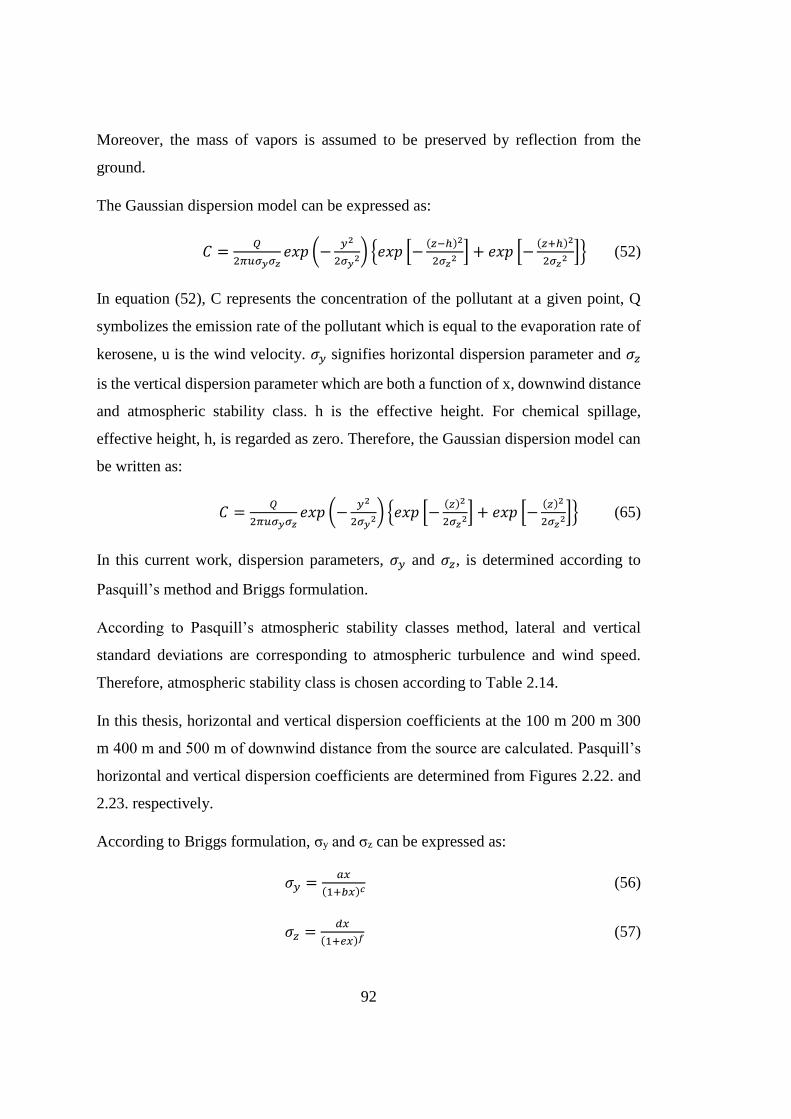
92

Moreover, the mass of vapors is assumed to be preserved by reflection from the

ground.

The Gaussian dispersion model can be expressed as:

𝐶 =𝑄

2𝜋𝑢𝜎𝑦𝜎𝑧𝑒𝑥𝑝 (−

𝑦2

2𝜎𝑦2) {𝑒𝑥𝑝 [−

(𝑧−ℎ)2

2𝜎𝑧2 ] + 𝑒𝑥𝑝 [−

(𝑧+ℎ)2

2𝜎𝑧2 ]} (52)

In equation (52), C represents the concentration of the pollutant at a given point, Q

symbolizes the emission rate of the pollutant which is equal to the evaporation rate of

kerosene, u is the wind velocity. 𝜎𝑦 signifies horizontal dispersion parameter and 𝜎𝑧

is the vertical dispersion parameter which are both a function of x, downwind distance

and atmospheric stability class. h is the effective height. For chemical spillage,

effective height, h, is regarded as zero. Therefore, the Gaussian dispersion model can

be written as:

𝐶 =𝑄

2𝜋𝑢𝜎𝑦𝜎𝑧𝑒𝑥𝑝 (−

𝑦2

2𝜎𝑦2) {𝑒𝑥𝑝 [−

(𝑧)2

2𝜎𝑧2] + 𝑒𝑥𝑝 [−

(𝑧)2

2𝜎𝑧2]} (65)

In this current work, dispersion parameters, 𝜎𝑦 and 𝜎𝑧, is determined according to

Pasquill’s method and Briggs formulation.

According to Pasquill’s atmospheric stability classes method, lateral and vertical

standard deviations are corresponding to atmospheric turbulence and wind speed.

Therefore, atmospheric stability class is chosen according to Table 2.14.

In this thesis, horizontal and vertical dispersion coefficients at the 100 m 200 m 300

m 400 m and 500 m of downwind distance from the source are calculated. Pasquill’s

horizontal and vertical dispersion coefficients are determined from Figures 2.22. and

2.23. respectively.

According to Briggs formulation, σy and σz can be expressed as:

𝜎𝑦 =𝑎𝑥

(1+𝑏𝑥)𝑐 (56)

𝜎𝑧 =𝑑𝑥

(1+𝑒𝑥)𝑓 (57)

93

In equation (56) and (57), a, b, c, d, e and f are experimental coefficients which are

chosen from Table 2.15. depending on meteorological and terrain data.

95

CHAPTER 5

5. RESULTS AND DISCUSSIONS

5.1. Results and Discussions for Evaporation Modelling

In evaporation modelling, it is necessary to calculate vapor pressure and mass transfer

constant. There are several different approaches for vapor pressure and mass transfer

constant calculation. Firstly, in this current thesis, four different model is applied for

vapor pressure calculation. Secondly, three different equations are used for mass

transfer constant determination. Finally, five evaporation models are applied to

calculate the evaporation rate of the JP-8 spill. All results are compared and most

suitable approaches are selected to be used in oil evaporation modelling regarding

physical and environmental conditions of the spill accident.

5.2. Vapor Pressure Calculation

In this current thesis, the vapor pressure of the JP-8 spill is calculated according to

Blokker’s, Fingas’, Jenkins’ and Tkalin’s model. Each model is used to obtain vapor

pressure of JP-8 spill at 30oC and vapor pressure line of kerosene versus varying

temperatures. The results of vapor pressure calculation are given in Table 5.1 and each

model application is discussed respectively.

Table 5.1. Vapor Pressure of Kerosene According to Various Models

Model Vapor Pressure mm Hg at 30 °C

Blokker 96,2842

Fingas 51,1439

Jenkins 6,5642

Tkalin 0,0109

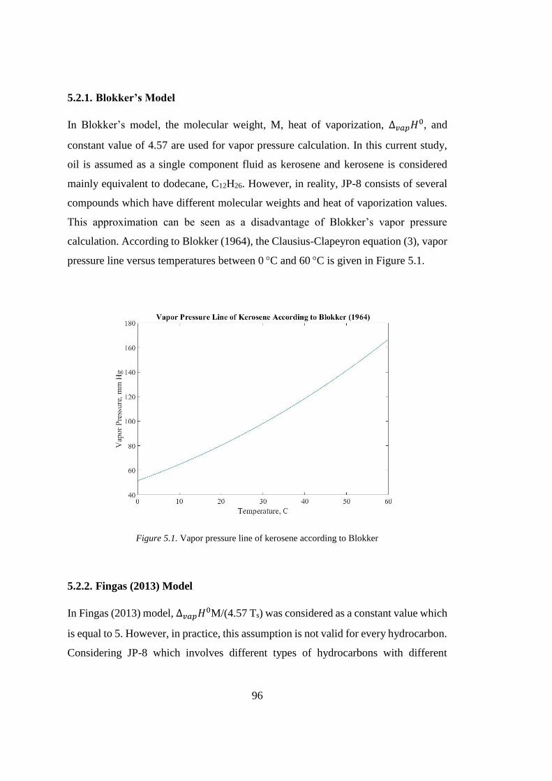
96

5.2.1. Blokker’s Model

In Blokker’s model, the molecular weight, M, heat of vaporization, ∆𝑣𝑎𝑝𝐻0, and

constant value of 4.57 are used for vapor pressure calculation. In this current study,

oil is assumed as a single component fluid as kerosene and kerosene is considered

mainly equivalent to dodecane, C12H26. However, in reality, JP-8 consists of several

compounds which have different molecular weights and heat of vaporization values.

This approximation can be seen as a disadvantage of Blokker’s vapor pressure

calculation. According to Blokker (1964), the Clausius-Clapeyron equation (3), vapor

pressure line versus temperatures between 0 °C and 60 °C is given in Figure 5.1.

Figure 5.1. Vapor pressure line of kerosene according to Blokker

5.2.2. Fingas (2013) Model

In Fingas (2013) model, ∆𝑣𝑎𝑝𝐻0M/(4.57 Ts) was considered as a constant value which

is equal to 5. However, in practice, this assumption is not valid for every hydrocarbon.

Considering JP-8 which involves different types of hydrocarbons with different

97

∆𝑣𝑎𝑝𝐻0M/(4.57 Ts) ratios, this approximation can be considered as a drawback of the

model. According to Fingas (2013), equation (4), vapor pressure line versus

temperatures between 0 °C and 60 °C is given in Figure 5.2.

Figure 5.2. Vapor pressure line of kerosene according to Fingas (2013)

5.2.3. Jenkins (2008) Model

In Jenkins (2008) model, heat of vaporization and gas constant is used for the vapor

pressure equation. In this study, since JP-8 is regarded as pure kerosene, heat of

vaporization of kerosene is used in calculation. Yet, JP-8 consists of different types of

compounds with different heat of vaporization values. This fact can be thought as the

downside of the model. According to Jenkins (2008), equation (7), vapor pressure line

versus temperatures between 0 °C and 60 °C is given in Figure 5.3.

98

Figure 5.3. Vapor pressure line of kerosene according to Jenkins (2008)

5.2.4. Tkalin’s Model

In Tkalin’s model, the boiling point of the oil product is used for vapor pressure

calculation. In this work, JP-8 is regarded as pure kerosene and the boiling point is

taken as 192 °C. In practice, the boiling point of the JP-8 can be different from the

boiling point of kerosene. This assumption can be regarded as the negative side of the

model. In addition, the pressure values obtained from the Tkalin model look very low

compared to other models. Therefore, Tkalin’s model is not suitable for evaporation

modeling of the JP-8 spill. According to Tkalin’s model, equation (25) and (26), vapor

pressure line versus temperatures between 0 °C and 60 °C is given in Figure 5.4.

Figure 5.4. Vapor pressure line of kerosene according to Tkalin’s Evaporation Model

99

5.3. Mass Transfer Constant Calculation

In this current work, the mass transfer constant of kerosene is determined according

to Mackay & Matsugu, Tkalin’s and Hamoda’s model. Each model is applied to mass

transfer constant calculation at spillage conditions. Mass transfer constant variation

graph is drawn with respect to different wind speeds and temperatures. The results of

mass transfer constant calculations are given in Table 5.2 and the results of each model

are discussed separately.

Table 5.2. Mass Transfer Constant of Kerosene According to Various Models

Model Mass Transfer

Constant m/s

Mackay & Matsugu 0,0084

Tkalin 0,0075

Hamoda 0,0021x10-3

5.3.1. Mackay & Matsugu Formulation for Mass Transfer Constant

In Mackay & Matsugu formulation, mass transfer constant is correspondent to wind

velocity, pool diameter and Schmidt number. As wind velocity increases mass transfer

constant also increases. Mackay & Matsugu formula yields K values similar to Tkalin

model. According to Mackay & Matsugu formulation, equation (9), K values versus

various wind velocities are given in Figure 5.5.

100

Figure 5.5. Mass Transfer Constant vs. Wind Speed According to Mackay&Matsugu (1973)

5.3.2. Hamoda Formulation for Mass Transfer Constant

In the Hamoda formula, mass transfer constant depends on API° density and

temperature. API° value is chosen as 44 which is the average of minimum and

maximum acceptable APIo density values at 60 °F given in Table 8. However, the

evaporation rate is calculated at 30 °C. This acceptance is the shortcoming of the

model. Moreover, the results of the mass transfer constant formula are very low

compared to other models. As a result, Hamoda formulation for mass transfer constant

calculation for oil JP-8 spill evaporation modeling is not significant. According to

Hamoda formula, equation (35), mass transfer constant versus temperatures between

0 °C and 60 °C is given in Figure 5.6.

101

Figure 5.6. Mass Transfer Constant vs. Temperature According to Hamoda et al. (1989)

5.3.3. Tkalin’s Formulation for Mass Transfer Constant

Tkalin’s formula for mass transfer constant calculation is very simple. In Tkalin’s

model, mass transfer constant is only correspondent to wind velocity. In the model,

mass transfer constant increases as wind velocity increases. The mass transfer constant

values found by Tkalin’s model is very similar to mass transfer constant values of

Mackay and Matsugu. According to Tkalin’s evaporation model, mass transfer

constant, K, in m/s, versus wind speed graph is given in Figure 5.7.

102

Figure 5.7. Mass Transfer Constant vs. Wind Speed According to Tkalin’s Evaporation Model

5.4. Evaporation Calculation

In this study, the evaporation rate of the JP-8 spill is calculated according to Stiver

and Mackay, Mackay and Wesenbeeck, Brighton, Tkalin and empirical equation

model. Five models are used to determine the evaporation rate at spill condition.

Evaporation rates are given in Table 5.3 and each evaporation model is argued

respectively.

Table 5.3. Evaporation Rate of JP-8 spill According to Various Models

Model Evaporation Rate kg/s

Stiver and Mackay 1,4366

Brighton 3,5722

Tkalin 97,3526

Mackay and Wesenbeeck 0,044

5.4.1. Stiver and Mackay Evaporation Model

In Stiver and Mackay evaporation model, the evaporation rate is related to mass

transfer constant, spillage area and vapor pressure. Mass transfer constant is

determined by Tkalin’s model. The vapor pressure of the JP-8 spill is calculated by

103

the Clausius-Clapeyron equation given in Jenkin (2008). The evaporation rate

obtained by Stiver and Mackay model is more lower than Brighton and Tkalin

evaporation models. Still, the heat of vaporization assumption of JP-8 can be different

from the value in practice. Additionally, JP-8 consists of several hydrocarbons so it is

expected that the evaporation rate is not a constant value. At the beginning of the spill,

more volatile hydrocarbons are expected to evaporate in high rates than less volatile

hydrocarbons evaporate slowly. Therefore, the JP-8 evaporation rate is expected to

decrease eventually.

5.4.2. Tkalin’s Evaporation Model

In Tkalin’s evaporation model, the evaporation rate is dependent on mass transfer

constant, molecular weight, vapor pressure, the amount of component and

temperature. Tkalin’s mass transfer approach results in sensible values. On the

contrary, Tkalin’s model for evaporation rate yields very high results for the JP-8 spill.

Additionally, the molecular weight of kerosene is considered similar to dodecane

however JP-8 consists of several hydrocarbon components. This weakness of the

model causes the model to yield very high evaporation rates. Additionally, Tkalin’s

model gives a constant evaporation rate for the JP-8 spill. Though, the JP-8

evaporation rate is expected to decrease as time increases. Thus, Tkalin’s evaporation

model is not appropriate for JP-8 spill evaporation modelling.

5.4.3. Brighton’s Evaporation Model

In Brighton’s evaporation model, the evaporation rate depends on mass transfer

constant, saturated vapor concentration at pool surface, wind velocity and pool

diameter. Mass transfer constant is calculated by Tkalin’s equation. Saturated vapor

concentration is dependent on the molecular weight and saturated vapor pressure of

kerosene. Saturated vapor pressure, which is determined by Jenkin’s model, is

104

proportional to the heat of vaporization. In this current work, assumed molecular

weight and heat of vaporization values of JP-8 can be different in practice since JP-8

consists of many different compounds. In addition, Brighton’s model yields a constant

evaporation rate which is not desired for oil evaporation modelling. These

assumptions can be seen as the handicaps of Brighton’s evaporation model. Thus,

Brighton’s evaporation model is not appropriate for JP-8 spill evaporation modelling.

5.4.4. Evaporation Modelling with Empirical Equation

In the empirical equation model, the evaporation rate is dependent on temperature and

time. According to the empirical evaporation equation, until the end of cleaning up of

JP-8 spill 40,7820% of the total amount of spillage evaporated which equals an

amount of 1.879,2345 kg. Evaporation rate decreases logarithmically and the highest

evaporation rate is obtained as 2,0074 kg/s in the third minute after the spill.

In reality, it is expected for the evaporation rate of JP-8 spill to decrease as time elapses

since more volatile hydrocarbons evaporate first and less volatile hydrocarbons

evaporate more slowly. Thus, the result of the empirical equation model is realistic.

However, in evaporation calculation, diesel long term empirical equation is chosen.

This assumption can be seen as a drawback for the model. It would be more accurate

to determine specific empirical equation for JP-8 evaporation calculation.

Additionally, emission rate is constant in vapor dispersion modelling. Therefore, a

constant evaporation rate is needed to be used in dispersion model. Percentage

evaporated and evaporation rate versus time graphs according to the empirical

equation model is given in Figure 5.8 and Figure 5.9 respectively.

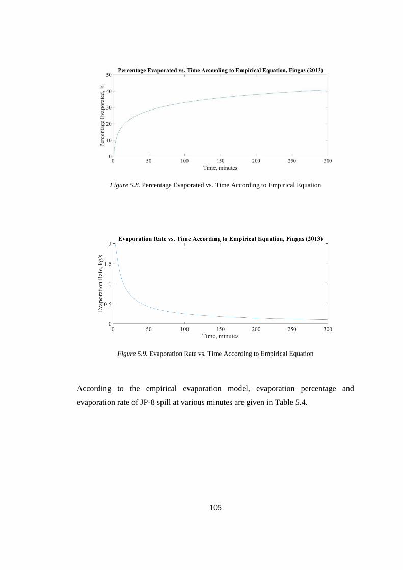
105

Figure 5.8. Percentage Evaporated vs. Time According to Empirical Equation

Figure 5.9. Evaporation Rate vs. Time According to Empirical Equation

According to the empirical evaporation model, evaporation percentage and

evaporation rate of JP-8 spill at various minutes are given in Table 5.4.

106

Table 5.4. Percentage Evaporated and Evaporation Rate at Various Time After Spill

t (minutes)

Percentage

Evaporated

%

Evaporation

Rate kg/s

2 4,9560 1,8998

3 7,8551 2,0074

4 9,9120 1,8998

8 14,8680 1,4249

17 20,2575 0,9136

22 22,1010 0,7702

33 25 0,5808

5.4.5. Mackay and Wesenbeeck Evaporation Model

Mackay and Wesenbeeck purposed an evaporation rate equation for dodecane as:

𝐸 = 474 × 𝑃 × 𝑀 (64)

In equation (64), E is the evaporation rate in µg/m2s, vapor pressure, P, is in Pa and

molar weight is in g/mol. The molecular weight of dodecane is 170 g/mol and vapor

pressure is 18,9763 Pa at 30 °C.

In Mackay and Wesenbeeck model, evaporation is correspondent to the molecular

weight and vapor pressure of dodecane. The vapor pressure of dodecane is calculated

by the Clausius-Clapeyron equation of Jenkins (2008). Saturated vapor pressure,

which is determined by Jenkin’s model, is proportional to the heat of vaporization. In

this study, the assumed molecular weight of dodecane and heat of vaporization values

can be a different value than JP-8 since JP-8 consists of several compounds. In

addition, Mackay and Wesenbeeck model yields a constant evaporation rate which is

the lowest value for oil evaporation modelling. These assumptions are the negative

side of the Mackay and Wesenbeeck model.

107

In literature, there are oil evaporation models concerning about oil spills at sea and

on soil. Wind has an mixing effect on oil spills at sea. On the other hand, in case of oil

spill on soil, oil is absorbed by soil. These cases have an effect on evaporation rate of

oil spill. However, these situations are not the concern for this current study.

Tkalin proposed an evaporation model for oil spills at sea. Oil spills at sea forms a

thin layer on sea surface. In Tkalin’s model, evaporation rate is correspondent to spill

amount. Therefore, all oil spill is subject to evaporation process. Yet, it is not the case

for oil spill accident in this study. In empirical equation model, evaporation rate

decreases logarithmically with time. However, in dispersion model it is needed to use

a constant evaporation rate. In Brighton model, evaporation rate calculation is derived

from the water evaporation model. In water evaporation, characteristics of the air layer

above the water surface has an effect on evaporation rate. Though, in oil evaporation,

evaporation rate is not affected by air boundary layer. Oil has different evaporation

mechanism from water. In Stiver and Mackay’s model, evaporation rate of oil is

dependent to vapor pressure. On the other hand, in Mackay and Wesenbeeck’

evaporation model, evaporation rate is correspondent to vapor pressure and molecular

weight but not only vapor pressure. This approach increases the prediction accuracy

for evaporation rate of the spilled substance.

In vapor dispersion modelling, Mackay and Wesenbeeck equation method is used to

calculate vapor concentrations as emission rate since it is considered as the best

suitable, easiest and most accurate approach.

5.5. Results and Discussions for Dispersion Modelling

In dispersion modelling, it is important to determine horizontal dispersion coefficient,

σy, and vertical dispersion coefficient, σz, according to downwind distance. Two

different methodology is used for dispersion coefficient determination. Results of two

methodologies are compared. After that, JP-8 vapor concentration dispersion is

calculated by using the Gaussian dispersion model.

108

5.5.1. Determination of σy and σz According to Pasquill’s Atmospheric Stability

Classes Method

In consideration of the information given in Table 4.1, insolation is slight and the wind

velocity is 5 m/s, atmospheric stability class is determined from Table 5.5 as D.

Table 5.5. Key to Stability Categories

Surface

wind

speed (at

10 m)

m/sec

Insolation Night

Strong Moderate Slight

Thinly

overcast or

≥4/8 low

cloud

≤3/8

cloud

<2 A A-B B - -

2-3 A-B B C E F

3-5 B B-C C D E

5-6 C C-D D D D

>6 C D D D E

For comparison of two methodologies, dispersion coefficients at the 100 m 200 m 300

m 400 m and 500 m of distance away from the source is calculated. According to

Pasquill’s method horizontal and vertical dispersion coefficients are determined from

Figures 5.10 and 5.11 respectively.

109

Figure 5.10. Horizontal dispersion coefficient, σy , vs. Downwind distance, x (Godish, 2004).

Figure 5.11. Vertical dispersion coefficient, σz , vs. Downwind distance, x (Godish, 2004).

110

According to Pasquill’s dispersion coefficient estimation model, 𝜎𝑦 and 𝜎𝑧, is

determined as in Table 5.6 given below:

Table 5.6. 𝜎𝑦 and 𝜎𝑧 Values According to Pasquill’s Model.

Downwind

Distance, x (m) σy (m) σz (m)

100 8 5.5

200 16 9.5

300 24 14

400 31 18

500 39 21

In Pasquill’s model, 𝜎𝑦 and 𝜎𝑧 values are determined by just looking at the graphs and

selected manually. This approach can lead to some accuracy errors in the

determination of dispersion coefficients.

5.5.2. Calculation of σy and σz According to Briggs Formulation

The stability class is determined as D and the terrain is rural. Therefore, experimental

coefficients of Briggs formula, a, b, c, d, e and f can be determined from Table 5.7 as

0.08, 0.0001, 0.5, 0.06, 0.0015 and 0.5 respectively.

111

Table 5.7. Experimental coefficients determined by Briggs

Rural

σy σz

Stability Class a b c d e f

A 0.22 0.0001 0.5 0.2 0 -

B 0.16 0.0001 0.5 0.12 0 -

C 0.11 0.0001 0.5 0.08 0.0002 0.5

D 0.08 0.0001 0.5 0.06 0.0015 0.5

E 0.06 0.0001 0.5 0.03 0.0003 1

F 0.04 0.0001 0.5 0.016 0.0003 1

Urban

σy σz

Stability Class a b c d e f

A-B 0.32 0.0004 0.5 0.24 0.0001 - 0.5

C 0.22 0.0004 0.5 0.2 0 -

D 0.16 0.0004 0.5 0.14 0.0003 0.5

E-F 0.11 0.0004 0.5 0.08 0.0015 0.5

According to Briggs dispersion coefficient formula, 𝜎𝑦 and 𝜎𝑧, is determined as in

Table 5.8 given below.

112

Table 5.8. 𝜎𝑦 and 𝜎𝑧 Values According to Briggs Formula

Downwind

Distance, x (m) σy (m) σz (m)

100 7.9603 5.5950

200 15.8424 10.5247

300 23.6479 14.9482

400 31.3786 18.9737

500 39.0360 22.6779

The comparison of the 𝜎𝑦 and 𝜎𝑧 values obtained from Paquill’s and Briggs’ model

are given in Table 5.9.

Table 5.9. Comparison of 𝜎𝑦 and 𝜎𝑧 Values According to Briggs Formula and Pasquill’s Method

Downwind

Distance, x (m)

σy (m)

σz (m)

Briggs Pasquill

Briggs Pasquill’s

100 7.9603 8 5.5950 5.5

200 15.8424 16 10.5247 9.5

300 23.6479 24 14.9482 14

400 31.3786 31 18.9737 18

500 39.0360 39 22.6779 21

According to Table 5.9, it can be seen that Pasquill and Briggs’ models result in close

values for 𝜎𝑦 and 𝜎𝑧. Therefore, both approaches can be used in oil vapor dispersion

models.

113

5.5.3. Application of Gaussian Dispersion Model

In dispersion modelling, emission source is assumed as ground level point source.

Gaussian Dispersion modelling is conducted by gaussianPlume MATLAB code which

is provided by Bien (2009).

In the Gaussian dispersion model, the distribution of JP-8 vapor concentration is

correspondent to emission rate, wind velocity, horizontal and vertical dispersion

coefficients. JP-8 vapors are dispersed through prevailing wind direction and diluted

as carried away from the source. The concentration distribution of JP-8 vapors is

Gaussian in the horizontal and vertical axis.

In order to determine the concentration levels of JP-8 vapors in the spill area, the

evaporation rate of the JP8 spill is taken as the emission rate in the dispersion

modeling. According to dispersion modeling, contour plots of the vapor concentration

of JP-8 regarding the spill accident scenario are given in Figure 5.12.

According to Figure 5.12, the vapor concentration of the JP-8 spill exceeds 7000 ppm

in a region of just below 0,4 meter height and up to 3 m downwind distance from the

source. Additionally, the vapor concentration of JP8 exceeds 30 ppm, TLV-TWA

value for kerosene, in a region of just below 2,6 meters height, up to 3,8 meters in both

vertical sides and up to 55 m downwind distance from the source in the prevailing

wind direction.

In Figure 5.12 it can be seen that flammable vapor concentration in the air reaches the

lower explosive limit (LEL) which is 0,7% by volume, 7000 ppm, in the air for

kerosene. Therefore, the explosive zone is formed and can be ignited by any kind of

ignition source. On the other hand, kerosene concentration exceeds the TLV-TWA

value of 30 ppm for a distance of 55 m from the spill in the wind direction. Also, vapor

concentration is well above the odor threshold of kerosene, 0.1 ppm, until 100 meters

away from the spill in the wind direction.

114

Figure 5.12. JP-8 Vapor Concentration vs. Downwind Distance

115

5.6. The Effect of Amount of Spill and Spillage Area

In Mackay and Wesenbeeck model, the evaporation rate is given as units of µg/m2s.

Therefore, the spillage area has an effect on the evaporation rate. According to Mackay

and Wesenbeeck evaporation equation, evaporation rate raises as the area of spill

increases.

In the empirical equation, the evaporation rate is correspondent to temperature and

time. Therefore, the amount of spill and spillage area has no effect on the dispersion

of the vapor concentration of the JP-8 spill.

Additionally, in the Brighton model, the evaporation rate is correspondent to pool

diameter. As pool diameter increases evaporation rate also increases. On the other

hand, in Stiver and Mackay model, the evaporation rate is in direct correlation with

the amount of spilled fuel and the spillage area.

Furthermore, in Tkalin’s model, the evaporation rate is dependent on the amount of

spill. As the amount of spill increases evaporation rate also increases. Accordingly,

higher evaporation rates result in higher JP-8 vapor concentration in the ambient air.

In case of constant spill area, such as spill into secondary containment pool, the

amount of spillage does not affect the evaporation rate. On the contrary, in the case of

open ground spillage, the spillage area is dependent on various factors such as the

shape of the surrounding terrain and the amount of spill. On flat terrain, a bigger

amount of spill causes liquid material to spread wider area so spill area increases as

the amount of spill increases. In this study, the spillage area is constant and the amount

of spill has no effect on the spillage area because of the secondary containment pool.

5.7. The Effect of Temperature

Temperature is an important parameter in evaporation calculation. In the empirical

equation model, the evaporation rate is directly proportional to temperature.

According to the empirical equation, in high temperatures, the percentage of

116

evaporation of the liquid substance will be higher. As a result, as temperature

increases, the evaporation rate also increases.

Mackay and Wesenbeeck evaporation model is directly proportional to vapor

pressure. The vapor pressure of a substance is dependent on temperature. As

temperature increases, vapor pressure also increases. Therefore, temperature has an

important effect on the vapor concentration of JP-8.

In dispersion modelling, the evaporation rate is taken as the emission rate of JP-8

vapors from the spillage. According to the Gaussian dispersion model, the vapor

concentration of JP-8 is directly proportional to the emission rate of vapors from the

spill. As a result, JP-8 vapor concentration in the air also increases as temperature

increases.

In order to see the effect of temperature on JP-8 vapors dispersion, dispersion model

is carried out at 10 °C and 40 °C ambient temperature. Results of JP-8 vapor dispersion

model for 10 °C and 40 °C is given in Figure 5.13 and Figure 5.14 respectively.

117

Figure 5.13. Vapor Concentration vs. Downwind Distance at 10 °C Temperature

118

Figure 5.14. Vapor Concentration vs. Downwind Distance at 40 °C Temperature

119

5.8. The Effect of Wind Speed in The Open Air

In the empirical equation model, the wind has no effect on the evaporation rate.

However, in Tkalin’s model, wind speed is used for mass transfer constant calculation.

According to Tkalin’s model, mass transfer constant increases with higher wind speed

values.

In Stiver and Mackay evaporation model, the evaporation rate is directly proportional

to mass transfer constant. In Stiver and Mackay model, mass transfer constant is

calculated according to Tkalin’s model. Since mass transfer constant is directly

proportional to wind velocity, an increase in mass transfer constant results in an

increased evaporation rate. On the contrary, in Mackay and Wesenbeeck evaporation

model, evaporation rate is independent of wind speed.

In dispersion modelling, as wind speed increases the JP-8 vapors disperse to more

distant location which causes lower values in concentration. On the other hand, in low

wind speed conditions, JP-8 vapor concentration is not diluted and reaches up to very

high concentration. Therefore, wind speed has a major effect on vapor concentrations

in dispersion modelling. Figures 5.15 and 5.16 show the vapor concentrations

distribution in downwind distance at 0.5 m/s and 6 m/s respectively.

120

Figure 5.15. Vapor Concentration vs. Downwind Distance at 0.5 m/s Wind Speed

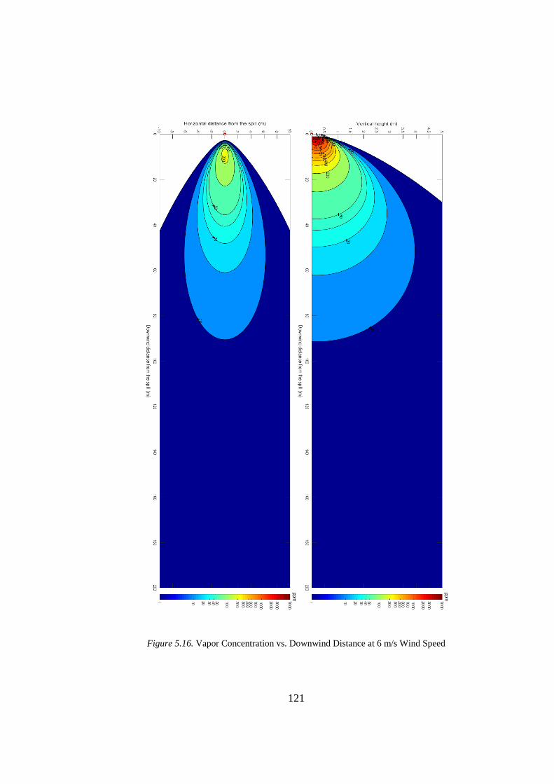
121

Figure 5.16. Vapor Concentration vs. Downwind Distance at 6 m/s Wind Speed

122

5.9. The Effect of Atmospheric Stability Class

The stability of weather increases from A class to F class. The most unstable weather

condition is A class, on the other hand, the most stable weather condition is F class.

In the Gaussian dispersion model, vapor concentrations are reversely proportional to

dispersion coefficients in both vertical and horizontal directions. In the unstable

weather condition, the JP-8 vapors disperse more in both vertical and horizontal

direction which causes lower vapor concentration. In contrast, in stable weather

conditions, dispersion will be lowered and concentation of JP-8 vapor is observed in

higher values.

5.10. The Effect of Land Characteristic

Land characteristic has an important effect on the dispersion of chemical vapors.

Structures on terrain can cause alteration in wind pattern which results in a change in

atmospheric stability.

As building height increases, wind moves upward direction causing an increase in

dispersion of JP-8 vapors. Therefore, in urban terrain, the vapor concentration of JP-

8 will be at lower levels.

5.11. Model Accuracy and Limitations

In this current thesis, two main models are used for the dispersion modelling of JP-8

vapors. Firstly, the evaporation rate of JP-8 is determined then the dispersion of JP-8

vapors is calculated.

In evaporation modelling, the vapor pressure of JP-8 is calculated according to a single

component liquid evaporation. However, in reality, JP-8 consists of many different

components. As the more volatile material evaporates first, the liquid composition will

change with time. As a result, the rate of evaporation will fall as evaporation proceeds.

123

Still, in this work, the evaporation rate is assumed as constant for four evaporation

models.

In mass transfer constant calculation according to Tkalin’ model, wind speed is

considered as constant. However, wind speed can vary during the evaporation process

which causes evaporation rate to fluctuate.

Additionally, the latent heat of vaporization varies with temperature. However, in this

study, the heat of vaporizations is taken as the value obtained from the kerosene

boiling point at 1 atm.

Furthermore, in this current study, it is assumed that there is no heat transfer occurs

between the oil, atmosphere and ground. Since oil temperature determines the vapor

pressure of kerosene, the evaporation rate of JP-8 will also be affected. In order to

obtain accurate evaporation modelling, it is very important to take heat transfer into

consideration.

In this current work, it is also assumed that the atmospheric turbulence is stationary

and homogeneous. Wind speed and direction are taken as constant during dispersion.

However, this assumption is not possible in practice. Atmospheric turbulence, wind

speed and direction change continuously which makes impossible to obtain accurate

dispersion prediction.

125

CHAPTER 6

6. CONCLUSION

Evaporation and dispersion modelling of oil spills is a very challenging subject. There

are many different models with some pros and cons. Every model can give different

results depending on the chemical and physical conditions of the oil spill. So, there is

no best model for evaporation and dispersion calculation of oil spillages. The most

important point in evaporation and dispersion estimation is to choose the most suitable

model according to the incident scenario. If appropriate evaporation and dispersion

model is applied to the oil spills, the vapor concentration prediction can be done

accurately. Otherwise, unrealistic modeling results can be encountered.

In mass transfer constant calculation, in contrast to Hamoda formula, Mackay and

Tkalin approaches yield almost similar results. Hamoda formula for mass transfer

constant calculation results in very low values compared to other models. Therefore,

Mackay and Tkalin model for mass transfer calculation is suitable for oil spill

evaporation modeling. Especially, Tkalin formulation for mass transfer constant is

very easy to apply if wind speed is known.

For vapor pressure calculation, four different vapor pressure calculation method is

applied to the spill of JP-8. Blokker, Fingas and Jenkins models are based on the

Clausius-Clapeyron equation expect from Tkalin’s model. Tkalin’ model for vapor

pressure calculation yields very low values. Therefore, Tkalin’s model is not suitable

for vapor pressure calculation in JP-8 spill evaporation modelling. On the other hand,

Blokker, Fingas and Jenkins models yield more realistic results. Blokker model gives

the highest value for vapor pressure, then Fingas and Jenkins models come

respectively. Since it is widely used and easy to apply, the Jenkins model is preferable

for vapor calculation in JP-8 spill evaporation modelling.

126

In evaporation modelling, Stiver and Mackay, Brighton, Tkalin, empirical model and

Mackay and Wesenbeeck model are used. Tkalin’s model results in very high values

so it is not applicable for JP-8 spill evaporation modelling. In contrast, Stiver and

Mackay, Brighton and empirical models yield acceptable evaporation rates. Brighton

model gives the highest evaporation rate for JP-8 evaporation, then Stiver and Mackay

and empirical method come respectively. The empirical equation gives logarithmic

curvature for the evaporation rate. However, in dispersion modelling, the emission

rate is needed to be constant. Since Mackay and Wesenbeeck model is easy to apply

and has higher accuracy, it is superior for evaporation modelling of JP-8 spill.

For vapor dispersion calculation, the Gaussian dispersion model is used. In the

Gaussian dispersion model, vapor concentrations have Gaussian distribution along the

horizontal and vertical axis. By using the Gaussian dispersion model, the variation of

vapor concentration from the maximum value to minimum value can be drawn as

contour plots. Also, the vapor concentration of the JP-8 spill can be specified at a

particular point in the downwind and crosswind position at a given time. According

to the Gaussian dispersion model, the highest vapor concentration is obtained in the

centerline of downwind direction where y is equal to zero.

According to JP-8 spill dispersion modelling, in the horizontal axis, the highest vapor

concentration reaches 200 ppm at a distance of 2 meters for both sides. Additionally,

the risk for the toxic health effect of JP-8 appears until 55 meters away from the spill

in the wind direction. After 55 meters away from the spillage, vapor concentrations

drop below 30 ppm which is TLV-TWA for kerosene. In the vertical axis over the

spill point, vapor concentrations exceed 7000 ppm which is LEL for kerosene.

Consequently, an explosion can occur in the presence of an ignition source in the

explosive zone. Furthermore, vapor concentration is well above the odor threshold of

kerosene, 0.1 ppm, more than 100 meters away from the spill in the wind direction.

In conclusion, the Gaussian dispersion model can be useful for determining the risk

level and possible outcomes of oil spill accidents. It is helpful to establish safe

127

operations in the aviation sector by clarifying the extent of hazards, understanding the

level of the risk of spill accidents. Additionally, it helps to predict the range of

explosive zone. Furthermore, evacuation zones can be declared in emergency response

plans for immediate evacuation during the spill accident. Therefore, by this current

study, ways of fast and efficient response to the oil spills can be determined and

adverse health effects of an oil spill to the public can be minimized in the aviation

sector.

129

CHAPTER 7

7. RECOMMENDATION

The main objective of the present work is to estimate the possible safety risks of the

JP-8 spill in the aviation sector. In order to evaluate possible outcomes of JP-8 spill

accident, evaporation and dispersion models are used. By using these models, the area

affected by the spill is revealed and the level of adverse effects is determined.

However, the models which are used in this current work have several limitations and

assumptions. The accuracy of evaporation and dispersion models can be decreased by

model limitations and assumptions.

In evaporation modelling, JP-8 is assumed as a pure substance which consists of

kerosene. Additionally, kerosene is assumed to have some similar molecular

properties with dodecane. In the evaporation rate calculation, the empirical

evaporation equation of dodecane is used. These assumptions lower the accuracy of

evaporation modeling. It is well-known that JP-8 contains many different chemicals

with different chemical and physical properties. In future studies, for obtaining more

accurate evaporation modelling results, the evaporation equation for JP-8 can be

determined empirically.

There are various different evaporation and dispersion models. Different models

should be applied to model dispersion of the JP-8 spill. So, the results of different

models can be compared and the most suitable approach can be decided more

accurately.

Evaporation and dispersion models requires a lot of data input and include complex

numbers for calculation. It can be useful to use computer programs for easily

predicting the concentration of chemical vapors emitted from the spill accident. So

130

that, important information can be obtained for the emergency response team for

understanding the level of the hazard and for clarifying the evacuation zone.

In the aviation industry, lots of chemicals are used in production and flight lines in

huge amounts. Because of this reason, similar modelling studies should be conducted

for other hazardous chemicals for assessment of safety risks and for determining safety

measures.

Spill accidents can happen in different climate conditions. Evaporation and dispersion

modelling should be conducted for different atmospheric conditions. Therefore, the

emergency response plan can be determined according to the worst-case scenario.

According to the dispersion model, within the area of 55 m radius from the oil spill,

buildings involving employees are needed to be evacuated immediately and entrance

to the spill area should be forbidden after the spill. TLV-TWA of kerosene is 30 ppm

and exposures above the TLV-TWA should not be allowed more than 15 minutes

otherwise adverse health effects can be observed.

In order to conduct safe fueling operations, safety instructions should be declared to

the operators. Necessary training should be given to operators. Operators without

training and knowledge should not be allowed to work at fueling stations. Operators

should be provided a dead man control unit in order to stop fueling operation in case

of emergency. Warning sign for explosive zone and static grounding should be present

at the station. Emergency phone numbers should be known by the operators and the

emergency call numbers should be hanged in the fuel station. Emergency response

plans should be documented and declared to operators. The emergency response team

should be determined, roles and responsibilities should be declared to team members.

Evacuation drills should be conducted regularly in the buildings close to the fueling

station.

During the fueling operations, access to the fueling areas should be limited. The fire

department should be noticed before the fueling operations and should be present at

the station during fueling. Fire extinguishers should be provided to the fuel station in

131

enough numbers. Fire alarm and smoke detection systems should be installed to fuel

station. For early response, hydrocarbon sensors detecting vapor concentrations can

be also installed to the fueling station. Also, installation of automatic blockage valves

for shutting the system down in case of system failure can prevent leakage.

The area where spill can occur and explosive zone can be formed, should be colored

to attract the attention of operators. In this zone, access to ignition sources should be

forbidden. In order to discharge static electricity, grounding plates should be replaced

at the fueling station. The outwear of operators should be made of antistatic material

to prevent static charging in the explosive zone. During fueling operation, aircraft and

fuel tanks should be connected and grounded.

133

REFERENCES

Abdel-Rahman, A. A. (2008). On the atmospheric dispersion and Gaussian plume

model. Proceedings of the 2nd International Conference on Waste Management,

Water Pollution, Air Pollution, Indoor Climate, pp. 31-39.

ACGIH (American Conference of Governmental Industrial Hygienists). (2015). 2015

TLVs and BEIs Based on the Documentation of the Threshold Limit Values for

Chemical Substances and Physical Agents and Biological Exposure Indices.

Cincinnati, OH: Signature Publications.

API (American Petroleum Institute). (2003). Ignition risk of hydrocarbon liquids and

vapors by hot surfaces in the open air (3rd ed., p. 3). Washington: American Petroleum

Institute.

Anfossi, D. and W. Physick (2004). Lagrangian Particle Models. Air Quality

Modeling – Theories, Methodologies, Computational Techniques, and Available

Databases and Software. Vol. II – Advanced Topics. The EnviroComp Institute and

the Air & Waste Management Association.

Artana, K. B., Pratiwi, E., Dinariyana, B., Pitana, T., Masroeri, A. A., Ariana, M.,

Arifin, M. D. (2014). Enhancement on Methodology for Estimating Emission

Distribution at Madura Strait by Integrating Automatic Identification System (AIS)

And Geographic Identification System (GIS), Proceedings of the 3rd International

Symposium of Maritime Sciences. Nov. 10-14, 2014, Kobe, Japan.

Baker, Q.A. et al. (2010). Guidelines for vapor cloud explosion, pressure vessel burst,

BLEVE, and flash fire hazards (2nd ed., p. 54). Hoboken, N.J: Wiley.

Beychok, M. R. (2005). Fundamentals of stack gas dispersion. Newport Beach, CA.

Bien, H. (2009). gaussianPlume [MATLAB Code]. Retrieved from

https://www.mathworks.com/matlabcentral/fileexchange/13279-

gaussianplume?s_tid=srchtitle

134

Bobra, M. (1992). A study of the evaporation of petroleum oils. Environment Canada,

Environmental Protection Directorate, River Road Environmental Technology Centre.

Boubel, R. W., Vallero, D., Fox, D. L., Turner, B., & Stern, A. C. (1994).

Fundamentals of air pollution. San Diego: Elsevier.

Brandt, J., Silver, J.D., Christensen, J.H., Andersen, M.S., Bønløkke, J.H., Sigsgaard,

T., Geels, C., Hansen, K.M., Kaas, E. and Frohn, L.M. (2014). Air Quality Effects on

Human Health. Air Pollution Modeling and its Application XXIII, pp. 7-15

Briggs G.A. (1973). Diffusion Estimation of Small Emissions. Contribution No. 79,

Atmospheric Turbulence and Diffusion Laboratory, Oak Ridge, TN.

Brighton, P. W. M. (1985). Evaporation from a plane liquid surface into a turbulent

boundary layer. Journal of Fluid Mechanics, 159(-1), 323.

Brighton, P. W. M. (1990). Further verification of a theory for mass and heat transfer

from evaporating pools. Journal of Hazardous Materials, 23(2), 215–234.

British Standards Institution (2008). Explosive atmospheres - Explosion prevention

and protection. London, U.K..

BP Process Safety Series (2006) - Hazards of Electricity and Static Electricity (6th

Edition). Institution of Chemical Engineers. Retrieved from

https://app.knovel.com/hotlink/toc/id:kpBPPSSHEI/bp-process-safety-series-2/bp-

process-safety-series-2

Chapman, H. (2017). "Performance Test of the Pasquill Stability Classification

Scheme". University of Wisconsin-Milwaukee. Retrieved from

http://dc.uwm.edu/etd/1453

Chickos, J.S. and Hanshaw, W. (2004). Vapor Pressures and Vaporization Enthalpies

of the n-Alkanes from C31 to C38 at T= 298.15 K by Correlation Gas

Chromatography. Journal of Chemical & Engineering Data, 49(3), 620-630.

135

Cooper, C.D. and Alley, F.C. (2011). Air Pollution Control, 4th ed., Long Grove:

Waveland Press.

Crowl, D. A. and Louvar, J. F. (2011). Chemical Process Safety Fundamentals with

Applications. 3rd ed. Upper Saddle River, NJ: Prentice Hall.

De Visscher, A. (2014). AIR DISPERSION MODELING Foundations and

Applications. Hoboken, New Jersey: John Wiley & Sons, Inc.

Deaves, D.M., Dense gas dispersion modelling. Journal of Loss Prevention in the

Process Industries Volume 5, Issue 4, 1992, Pages 219-227.

Drivas, P.J., "Calculation of Evaporative Emissions from Multicomponent Liquid

Spills", Environmental Science and Technology, Vol. 16, pp. 726-728, 1982.

Environmental Protection Agency (EPA), (2002). Dense Gas Dispersion Model

(DEGADIS). (2002, December 10). Retrieved January 14, 2019, from

https://cfpub.epa.gov/si/si_public_record_Report.cfm?Lab=&dirEntryID=2904

Federal Aviation Administration (FAA), (2008). Aviation Maintenance Technician

Handbook – General. Washington: U.S. Government Printing Office (GPO).

Retrieved April 10, 2019, from

https://www.faa.gov/regulations_policies/handbooks_manuals/aircraft/

Fingas, M.F. (1995). "A Literature Review of the Physics and Predictive Modelling

of Oil Spill Evaporation", Journal of Hazardous Materials, Vol. 42, pp.157-175, 1995.

Fingas, M. (1996). The evaporation of oil spills: Prediction of equations using

distillation data. Spill Science & Technology Bulletin, 3(4), 191–192.

136

Fingas, M.F. (1997). "Studies on the Evaporation of Crude Oil and Petroleum

Products: I. The Relationship between Evaporation Rate and Time", Journal of

Hazardous Materials, Vol. 56, pp. 227-236, 1997.

Fingas, M.F. (1998). “Studies on the evaporation of crude oil and petroleum products

II. Boundary layer regulation”, Journal of Hazardous Materials, Volume 57, Issues 1–

3, January 1998, Pages 41-58.

Fingas, M. F. (1999). The Evaporation of Oil Spills: Development and

Implementation of New Prediction Methodology. International Oil Spill Conference

Proceedings: March 1999, Vol. 1999, No. 1, pp. 281-287.

Fingas, M. F. (2001). The Basics of Oil Spill Cleanup. (2.nd ed., pp.) Boca Raton:

Lewis Publishers.

Fingas, M. F. (2004). Modeling evaporation using models that are not boundary-layer

regulated, Journal of Hazardous Materials, Volume 107, Issues 1–2, Pages 27-36.

Fingas, M. F. (2011a). Oil and Petroleum Evaporation. J. Pet. Sci. Res. 2. 426-459.

Fingas, M. F. (2011b). Oil Spill Science and Technology - Prevention, Response, and

Cleanup. Burlington: Elsevier.

Fingas, M. F. (2013). “Modeling Oil and Petroleum Evaporation”, Journal of

Petroleum Science Research (JPSR), Vol. 2, pp. 104-115, Issue 3, July 2013.

Ghassemi, H., Baek, S. W., & Khan, Q. S. (2006). Experimental Study On

Evaporation Of Kerosene Droplets At Elevated Pressures And Temperatures.

Combustion Science and Technology, 178(9), 1669–1684.

Godish, T. (2004). Air Quality. (4th ed., pp.78-79). Boca Raton: Lewis Publishers.

137

Goodwin, S. R., Mackay, D., & Shiu, W. Y. (1976). Characterization of the

evaporation rates of complex hydrocarbon mixtures under environmental conditions.

The Canadian Journal of Chemical Engineering, 54(4), 290–294.

Groh, H. (2004). Explosion protection (pp. 8-10). Amsterdam: Elsevier/Butterworth

Heinemann.

Haghighi, E., E. Shahraeeni, P. Lehmann, and D. Or (2013), Evaporation rates across

a convective air boundary layer are dominated by diffusion, Water Resour. Res.,

Volume49, Issue3, March 2013 Pages 1602-1610

Hamoda, M. F., Hamam, S. E. M., & Shaban, H. I. (1989). Volatilization of crude oil

from saline water. Oil and Chemical Pollution, 5(5), 321–331.

Hanna, R. S., Briggs, G. A., Hosker, R. P. (1982). Handbook on Atmospheric

Diffusion. U.S.: Technical Information Center, U.S. Department of Energy.

Harrop, O. D. (2002). Air Quality Assessment and Management - A Practical Guide.

London: Spon Press.

Hattwig, M., & Steen, H. (2004). Handbook of Explosion Prevention and Protection

(p. 5). Weinheim: Wiley-VCH.

Indra, E., Sinha, N., Ghose, M. K., Singh, G., Srivastava, S., Sinha, I., (2004).

Classification of air pollution dispersion models: a critical review. Proceedings of the

National Seminar on Environmental Engineering with special emphasis on Mining

Environment. pp. 19-20.

Jenkins, H. D. B. (2008). Chemical Thermodynamics at a Glance. Oxford, England:

Blackwell.

John Duffy Energy Services. (2006). Material Safety Data Sheet (MSDS) - Kerosene

1-K Dyed. Retrieved from http://duffyenergy.com/dev-site-duffyenergy-2015/wp-

content/uploads/2015/07/Kerosene-MSDS.pdf

138

Lim, S. S., Vos, T., Flaxman, A. D., Danaei, G., Shibuya, K., Adair-Rohani, H., &

Aryee, M. (2012). A comparative risk assessment of burden of disease and injury

attributable to 67 risk factors and risk factor clusters in 21 regions, 1990–2010: a

systematic analysis for the Global Burden of Disease Study 2010. The Lancet,

380(9859), pp. 2224-2260.

Lin, J. C. (2012). Lagrangian Modeling of the Atmosphere: An Introduction.

Washington, DC: Geopress

Lüttgens, G., Lüttgens S. and Schubert W. (2017). Static Electricity. Weinheim,

Germany: Wiley-VCH

Mackay, D. and Matsugu, R. S. (1973), Evaporation rates of liquid hydrocarbon spills

on land and water. Can. J. Chem. Eng., 51: 434-439.

Mackay, D., & Wesenbeeck, I. V. (2014). Correlation of Chemical Evaporation Rate

with Vapor Pressure. Environmental Science & Technology, 48(17), 10259–10263.

Mannan, S. (2014). Lees' process safety essentials (p. 218). Amsterdam: Elsevier,

Butterworth-Heinemann.

Markiewicz, M. T. (2006). Modeling of the air pollution dispersion. MANHAZ

monograph, models and techniques for health and environmental hazard assessment

and management. pp.303-348

Martin, D. O. (1976). Comment on the change of concentration standard deviations

with distance. Journal of the Air Pollution Control Association, 26:2, 145-147.

Monteith, J. L. and Unsworth, M. H., (2013) Principles of Environmental Physics

Plants, Animals, and the Atmosphere, Fourth Edition (4th ed., p. 135). San Diego:

Elsevier.

139

Moosemiller, M. (2014). Guidelines for determining the probability of ignition of a

released flammable mass (p. 9). Hoboken, NJ: Wiley.

Namdeo, A., Sohel, I., Cairns, J., Bell, M., Khare, M., Nagendra, S., (2012).

Performance evaluation of air quality dispersion models in Delhi, India. Urban

Environment: Proceedings of the 10th Urban Environment Symposium, pp. 121-130

Nesaratnam, S. and Taherzadeh, S. (2014). Air Quality Management. Chichester: John

Wiley & Sons Ltd.

Nolan, D. (2014). Handbook of Fire and Explosion Protection Engineering Principles,

3rd Edition (3rd ed., p. 441). Eastbourne: Elsevier Science and Technology Books,

Inc.

National Fire Protection Association (NFPA), (2003a). Code for Motor Fuel

Dispensing Facilities and Repair Garages (2003 ed.).

National Fire Protection Association (NFPA), (2003b). Flammable and Combustible

Liquids Code (2003 ed.).

Pasquill, F. “The Estimation of the Dispersion of Windborne Material”,

Meteorological Magazine, Vol. 90, pp.33 – 49, 1961.

Purser, D. A., Maynard, R. L., Wakefield, J.C. (2016). Toxicology, Survival and

Health Hazards of Combustion Products. Cambridge, UK: Royal Society of Chemistry

Reijnhart, R., & Rose, R. (1982). Evaporation of crude oil at sea. Water Research,

16(8), 1319–1325.

Quinn, M. F., Marron, K., Patel, B., Abu-Tabanja, R., & Al-Bahrani, H. (1990).

Modelling of the ageing of crude oils. Oil and Chemical Pollution, 7(2), 119–128.

140

Roth, D., Sharma, P., Haeber, T., Schiessl, R., Bockhorn, H., & Maas, U. (2014).

Ignition by Mechanical Sparks: Ignition of Hydrogen/Air Mixtures by Submillimeter-

Sized Hot Particles. Combustion Science and Technology, 186(10-11), 1606-1617.

Russell, A., Holmes, H., Friberg, M., Ivey, C., Hu, Y., Balachandran, S., Mulholland,

J., Tolbert, P., Sarnat, J., Sarnat, S., Strickland, M., Chang, H. and Liu, Y., (2014).

Use of Air Quality Modeling Results in Health Effects Research. Air Pollution

Modeling and its Application XXIII, pp. 1-4

Schaschke, C. (2014). Dictionary of Chemical Engineering. Oxford, U.K.: Oxford

University Press.

Singh, K. (2018). Air pollution modelling. International Journal of Advance Research,

Ideas and Innovations in Technology, 4(3), pp. 951-959.

Speight, J. G. (2011). Handbook of Industrial Hydrocarbon Processes. Burlington:

Gulf Professional Publishing.

Speight, J. G. (2014). The Chemistry and Technology of Petroleum. 5th ed. Boca

Raton: CRC Press.

Speight, J. G. (2017). Rules of Thumb for Petroleum Engineers. Hoboken: John Wiley

& Sons.

Speight, J. G. and El-Gendy, N. S. (2018). Introduction to Petroleum Biotechnology.

Cambridge: Gulf Professional Publishing.

Spellman, F. R. and Stoudt, M. L. (2013). Environmental Science: Principles and

Practices. Lanham: Scarecrow Press, Inc.

Spicer, T. and Havens, J. (1989). User’s Guide for the DEGADIS 2.1 Dense Gas

Dispersion Model. North Carolina: EPA.

141

Sriram, G., Mohan, N. K., & Gopalasamy, V. (2006). Sensitivity study of Gaussian

dispersion models. Journal of Scientific & Industrial Research Vol.65, pp. 321-324.

Stiver, W. and Mackay, D. (1984). "Evaporation Rate of Spills of Hydrocarbons and

Petroleum Mixtures". Environmental Science and Technology, Vol. 18, pp. 834-840.

Sutherland, A. R. & Hansen, V. F. & Bach, D. W. (1986). A quantitative method for

estimating Pasquill stability class from windspeed and sensible heat flux density.

Boundary-Layer Meteorology, 37, pp.357-369.

Thermo Fisher Scientific. (2018). Safety Data Sheet (SDS) – n-Dodecane. Retrieved

from

https://www.fishersci.com/msdsproxy%3FproductName%3DO2666500%26product

Description%3DN-DODECANE%2BP%2B500ML%26catNo%3DO2666-

500%2B%26vendorId%3DVN00033897%26storeId%3D10652

Turner, D.B. (1994). Workbook of Atmospheric Dispersion Estimates, 2nd Ed., Boca

Raton: Lewis Publishers.

Totten, G. E., Westbrook, S. R., Shah, R. J. (2003). Fuels and Lubricants Handbook -

Technology, Properties, Performance, and Testing. West Conshohocken: ASTM

International.

United States Air Force (USAF), (2013). Ground Servicing of Aircraft and Static

Grounding/Bonding. Warner Robins: USAF.

United States Air Force (USAF), (2016). Concurrent Fuel Servicing of Commercial

Contract Cargo and Passenger Aircraft. Warner Robins: USAF.

United States Air Force (USAF), (2018). Air Force Manual 91-203: Air Force

Occupational Safety, Fire and Health Standards.

142

United States Department of Defense, (2015). MIL-DTL-83133E, Detail

Specification: Turbine Fuel, Aviation, Kerosene Type, JP-8 (NATO F-34), NATO F-

35, and JP-8+100 (NATO F-37).

Valdenebro, V., Sáez de Cámara, E., Gangoiti, G., Alonso, L., García, J.A., Ilardia,

J.L., González, N. and Arraibi, E. (2014). The Use of a Mesoscale Modeling System

Together with Surface and Upper Observational Data to Estimate Hourly Benzene

Impacts in a Mountainous Coastal Area. Air Pollution Modeling and its Application

XXIII, pp. 535-538.

Vallero, D. (2014). Fundamentals of Air Pollution. 5th ed., San Diego: Elsevier.

Vinnem, J. (2014). Offshore Risk Assessment vol 1 Principles, Modelling and

Applications of QRA Studies. (3rd ed., p. 275). London, U.K.: Springer.

Walcek C. J. (2002). Lagrangian vs. eulerian dispersion modelling: effects of wind

shear on pollution dispersion, 12th Joint Conference on the Applications of Air

Pollution Meteorology with the Air and Waste Management Association, American

Meteorological Society.

Wang, M. (2019). Understandable Electric Circuits - Key Concepts (2nd Edition).

London, U.K.: Institution of Engineering and Technology.

Weber, E. (1982). Air Pollution Assessment Methodology and Modeling. New York:

Springer Science+Business Media.

Woodward, J. L. (1998). Estimating the Flammable Mass of a Vapor Cloud (p. xvii).

New York, N.Y.: Center for Chemical Process Safety of the American Institute of

Chemical Engineers.

Yang, W. C., & Wang, H. (1977). Modeling of oil evaporation in aqueous

environment. Water Research, 11(10), 879–887.

143

Yuan, Y., Yang, K., Du, C., Fu, X. (2017), Study on Schmidt Number of Pollutant

Diffusion in Urban Street Atmosphere, Procedia Engineering, Volume 205, Pages

1711-1717.

Zannetti P. (1990) Lagrangian Dispersion Models. In: Air Pollution Modeling.

Boston, MA: Springer.

Zapert, J. P., Londergan R. J. and Thistle, H. (1991). Evaluation of Dense Gas

Simulation Models. North Carolina: EPA.