Dispersal Conditions and Assimilative Capacity of Air ...ijsrset.com/paper/366.pdfEnvironment at...
11
IJSRSET151382 | Received: 30 June 2015 | Accepted: 08 July 2015 | July-August 2015 [(1)4: 05-15] © 2015 IJSRSET | Volume 1 | Issue 4 | Print ISSN : 2395-1990 | Online ISSN : 2394-4099 Themed Section: Science 5 Dispersal Conditions and Assimilative Capacity of Air Environment at Gajuwaka Industrial Hub in Visakhapatnam Srinivasa Rao S, N. Srinivasa Rajamani, E. U. B. Reddi Department of Environmental Sciences, Andhra University, Visakhapatnam, Andhra Pradesh, India ABSTRACT The comprehension of a pollution event requires not only the accurate determination of the chemical composition of the atmospheric particles but also the elucidation of the role played by the dilution properties of the lower atmosphere. In this context, a rapidly growing Gajuwaka industrial hub in Visakhapatnam was chosen for estimating the assimilative capacity of air environment for its pollution potential by calculating the ventilation coefficient values. The diurnal variations of assimilation capacity of atmosphere were shown high during the noon hours and low at night and early morning hours in all the seasons. The monthly variations of low and high assimilative capacities were observed in the month of February and October respectively. Seasonally, post- monsoon showed high ventilation capacity followed by monsoon, winter and pre-monsoon seasons. Further, this is compared with the seasonal variations of the ambient air quality at the study area. The study area met the criteria of low pollution potential for all the time except for morning hours. The study area exhibited ‘good’ category dispersal conditions with an annual mean of ventilation coefficient value of 4271.6m2s-1 and the duration of ‘good’ dispersal conditions are longer in the months of April, May and June compared to other seasonal months. Keywords: Pollution potential, Ventilation coefficient, Mixing heights, Transport winds I. INTRODUCTION Urbanization and industrialization growth at any stage has direct impact on the surrounding air quality due to prevailed pollutants. The increase in the air concentration of a pollutant, in fact, is the result of the combination of the emission (and/or production) of the pollutants in the atmosphere and of the reduced capacity of the atmosphere to dilute them [1]. In the present situation of developmental activities, when new industries are coming up and the existing ones increasing their capacities, it is necessary to study the assimilative/healing capacity of the particular area to estimate the carrying capacity. The assimilative capacity of the atmosphere gives roughly an idea of the extent to which the atmosphere is capable of sustaining the pollution load from various emission sources [2]. Application of meteorological phenomena is well known to determine the assimilative capacity for a locality. The assimilative capacity of the atmosphere is determined in terms of ventilation coefficient, which is the product of two meteorological parameters, mixing height and average wind speed through mixing heights (transport wind speed). The assimilative capacity of the atmosphere is directly proportional to the ventilation coefficient and inversely proportional to the pollution potential [3]. Dispersal conditions of pollutants at coastal regions are of great concern because of typical meteorological features of the lower atmosphere. Understanding the dispersal conditions and assimilative capacity of air environment can be useful for planners/technologists to mitigate air pollution events. In view of the above, rapidly growing Gajuwaka industrial hub of Visakhapatnam was chosen for the present study. A. Topography and Prevailing Meteorology of the Gajuwaka Industrial Hub – The Study Area It is located on the south of Visakhapatnam city in between 17 0 34’00” N to 17 0 42’00” N latitudes and 83 0 06’00” E to 83 0 14’00” E longitudes were chosen for the present study. The present study area is not situated in
Transcript of Dispersal Conditions and Assimilative Capacity of Air ...ijsrset.com/paper/366.pdfEnvironment at...

IJSRSET151382 | Received: 30 June 2015 | Accepted: 08 July 2015 | July-August 2015 [(1)4: 05-15]
© 2015 IJSRSET | Volume 1 | Issue 4 | Print ISSN : 2395-1990 | Online ISSN : 2394-4099 Themed Section: Science
5
Dispersal Conditions and Assimilative Capacity of Air
Environment at Gajuwaka Industrial Hub in Visakhapatnam
Srinivasa Rao S, N. Srinivasa Rajamani, E. U. B. Reddi
Department of Environmental Sciences, Andhra University, Visakhapatnam, Andhra Pradesh, India
ABSTRACT
The comprehension of a pollution event requires not only the accurate determination of the chemical composition
of the atmospheric particles but also the elucidation of the role played by the dilution properties of the lower
atmosphere. In this context, a rapidly growing Gajuwaka industrial hub in Visakhapatnam was chosen for
estimating the assimilative capacity of air environment for its pollution potential by calculating the ventilation
coefficient values. The diurnal variations of assimilation capacity of atmosphere were shown high during the noon
hours and low at night and early morning hours in all the seasons. The monthly variations of low and high
assimilative capacities were observed in the month of February and October respectively. Seasonally, post-
monsoon showed high ventilation capacity followed by monsoon, winter and pre-monsoon seasons. Further, this
is compared with the seasonal variations of the ambient air quality at the study area. The study area met the
criteria of low pollution potential for all the time except for morning hours. The study area exhibited ‘good’
category dispersal conditions with an annual mean of ventilation coefficient value of 4271.6m2s-1 and the
duration of ‘good’ dispersal conditions are longer in the months of April, May and June compared to other
seasonal months.
Keywords: Pollution potential, Ventilation coefficient, Mixing heights, Transport winds
I. INTRODUCTION
Urbanization and industrialization growth at any stage
has direct impact on the surrounding air quality due to
prevailed pollutants. The increase in the air
concentration of a pollutant, in fact, is the result of the
combination of the emission (and/or production) of the
pollutants in the atmosphere and of the reduced capacity
of the atmosphere to dilute them [1]. In the present
situation of developmental activities, when new
industries are coming up and the existing ones
increasing their capacities, it is necessary to study the
assimilative/healing capacity of the particular area to
estimate the carrying capacity. The assimilative capacity
of the atmosphere gives roughly an idea of the extent to
which the atmosphere is capable of sustaining the
pollution load from various emission sources [2].
Application of meteorological phenomena is well known
to determine the assimilative capacity for a locality. The
assimilative capacity of the atmosphere is determined in
terms of ventilation coefficient, which is the product of
two meteorological parameters, mixing height and
average wind speed through mixing heights (transport
wind speed). The assimilative capacity of the
atmosphere is directly proportional to the ventilation
coefficient and inversely proportional to the pollution
potential [3]. Dispersal conditions of pollutants at
coastal regions are of great concern because of typical
meteorological features of the lower atmosphere.
Understanding the dispersal conditions and assimilative
capacity of air environment can be useful for
planners/technologists to mitigate air pollution events. In
view of the above, rapidly growing Gajuwaka industrial
hub of Visakhapatnam was chosen for the present study.
A. Topography and Prevailing Meteorology of the
Gajuwaka Industrial Hub – The Study Area
It is located on the south of Visakhapatnam city in
between 170 34’00” N to 17
0 42’00” N latitudes and 83
0
06’00” E to 830 14’00” E longitudes were chosen for the
present study. The present study area is not situated in

International Journal of Scientific Research in Science, Engineering and Technology (ijsrset.com)
6
the bowl area of Visakhapatnam. The study area has
seen rapid industrialization and tremendous population
growth during the last few decades. It is spread over an
area of 97 km2 with a total population of about 3,70,000
(provisional figures of 2011 census) and with a semi
urban and rural atmosphere. The study area encompasses
with a thermal power plant, upcoming pharma city, an
integrated steel plant, a minor port, a number of
associated ancillaries and bound in the east by the Bay
of Bengal (Fig.1). The topography of the area is from
plain to undulating with small hillocks. Yarada hill
range stretches from E to WNW and NW of the study
area with a maximum altitude of about 360m. The
climate is warm and humid. This area experiences two
spells of rainfall during the southwest and northeast
monsoons. In addition, this area is subjected to on an
average two to three low pressure depressions
(sometimes intensified to cyclonic storms) which results
in moderate to heavy rains. The winds are north-
northeasterly during the winter season while during the
summer they are west- southwesterly and variations in
wind directions were observed due to the effect of land
and sea breeze. Wind speed is quite high with
predominant wind direction of WSW followed by W and
SW. Diurnal variation in wind speed showed that the
speed was high during daytime reaching a maximum at
around 14:00–16:00hrs and gradually decreasing with
nightfall reaching a minimum at midnight. A maximum
calm conditions frequency of 73% was observed at
04:00hrs during winter season.
II. METHODS AND MATERIAL
For ventilation coefficient calculations, surface wind
speed data were collected from the weather monitoring
station located in the study area and monthly averages of
hourly observations of mixing heights (Z1) were
obtained from the reports (the data of Visakhapatnam) of
National Environmental Engineering Research Institute,
Nagpur [4] as the study area specific mixing heights
were not available and the data of Visakhapatnam was
adopted which is very close (16kms) to this study area.
Then the monthly averages of hourly wind speed
observations based on available data during three years
period (2008-2010) have been calculated for monthly
averages of hourly transport wind speed (U1) by
applying the wind profile (power) law [5].
Ventilation Coefficient (m2s
-1) = Z1U1
Where
Z1 = mixing height,
U1 = average wind speed in the mixed
height (transport wind speed).
By applying the above equation, hourly, monthly with
seasonal and annual ventilation coefficients have been
calculated for the study area. Further, the following
criteria have been considered to delineate the pollution
potential for this present study;
1) The US National Meteorological Centre and
Atmospheric Environment Services, Canada, has
classified that high pollution potential occurs when
the afternoon ventilation coefficient is <6000m2s
-1
and transport wind speed does not exceed 4m/s and
during morning hours, the mixing height is <500m
and transport wind speed does not exceed 4 m/s
and the winds at a height of 1500m must average
less than 10m/s [6, 7].
2) The air pollution dispersion index (ventilation
index) which is proposed by the State of Colorado
Department of Health in Denver is used to
categorize as POOR: 0-2000m2s
-1, FAIR: 2001-
4000m2s
-1, GOOD: 4001-6000m
2s
-1 and
EXCELLENT: >6001m2s
-1 [8, 9]. Lower values of
ventilation coefficient indicate less dispersion
potential of pollutants where as higher value
designates the capacity of the atmosphere to disperse
the pollutants.
Keeping in view the importance of the study area,
ambient air quality monitoring was carried out at some
selected residential colonies during winter and summer
seasons for a period of two years (2008-2010).
Subsequently, the measured data of six criteria air
pollutants were converted into an Indian air quality
index (IND-AQI) recently developed by CPCB, New
Delhi, (http://home.iitk.ac.in/~mukesh/air-quality/
Basis.html) to compare the seasonal variations of the air
quality with respect to assimilative capacity of the study
area.
III. RESULTS AND DISCUSSION
The calculated monthly averages of hourly ventilation
coefficients (VC) values and the related mixing heights
during different seasons were presented in figures 2 - 13.
International Journal of Scientific Research in Science, Engineering and Technology (ijsrset.com)
7
Further, monthly and seasonal variations of ventilation
coefficient values were presented in Fig. 14 to delineate
status of the study area. Seasonal and annual frequency
of hourly dispersal conditions at the study area was
presented in Fig. 15 to appreciate the pollution potential.
Annual mean of IND-AQI values and seasonal
variations of pollutants at the study area were shown in
Fig.16 and 17 respectively.
A. Ventilation coefficient (VC) values during pre-
monsoon period
From the above figures, it can be noted that the fall of
ventilation coefficient values at the time of noon hours
was leading to high pollution potential for a short while.
Again, the increase of values revealed the good dispersal
conditions at the study area. These fluctuations can be
attributed to the meso scale meteorological features at
the study area. Higher and lower values were observed
during 08-09:00 and 03-06:00hrs respectively. On an
average, the month of May exhibited ‘good’ dispersal
conditions (4514.8m2s
-1) when compared with the other
two months showing ‘fair’ dispersal conditions.
Fig. 2: Averages of hourly ventilation coefficient (VC) & mixing height (MH) values in the month of March.
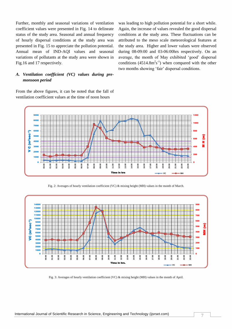
Fig. 3: Averages of hourly ventilation coefficient (VC) & mixing height (MH) values in the month of April.
0
200
400
600
800
1000
1200
0
1000
2000
3000
4000
5000
6000
7000
8000
9000
00:0
0
01:0
0
02:0
0
03:0
0
04:0
0
05:0
0
06:0
0
07:0
0
08:0
0
09:0
0
10:0
0
11:0
0
12:0
0
13:0
0
14:0
0
15:0
0
16:0
0
17:0
0
18:0
0
19:0
0
20:0
0
21:0
0
22:0
0
23:0
0
M H
(m
)
V C
(m
2se
c-1)
Time in hrs VC MH
0
100
200
300
400
500
600
700
800
900
0
1000
2000
3000
4000
5000
6000
7000
8000
9000
10000
11000
12000
13000
14000
00:0
0
01:0
0
02:0
0
03:0
0
04:0
0
05:0
0
06:0
0
07:0
0
08:0
0
09:0
0
10:0
0
11:0
0
12:0
0
13:0
0
14:0
0
15:0
0
16:0
0
17:0
0
18:0
0
19:0
0
20:0
0
21:0
0
22:0
0
23:0
0
MH
(m
)
VC
(m
2se
c-1)
Time in hrs.
VC MH

International Journal of Scientific Research in Science, Engineering and Technology (ijsrset.com)
8
Fig. 4: Averages of hourly ventilation coefficient (VC) & mixing height (MH) values in the month of May
Fig. 5: Averages of hourly ventilation coefficient (VC) & mixing height (MH) values in the month of June.
Fig. 6: Averages of hourly ventilation coefficient (VC) & mixing height (MH) values in the month of July.
0
100
200
300
400
500
600
700
800
900
0
1000
2000
3000
4000
5000
6000
7000
8000
9000
10000
11000
12000
13000
00:0
0
01:0
0
02:0
0
03:0
0
04:0
0
05:0
0
06:0
0
07:0
0
08:0
0
09:0
0
10:0
0
11:0
0
12:0
0
13:0
0
14:0
0
15:0
0
16:0
0
17:0
0
18:0
0
19:0
0
20:0
0
21:0
0
22:0
0
23:0
0
MH
(m
)
VC
(m
2se
c-1)
Time in hrs.
VC MH
0
100
200
300
400
500
600
700
800
0
1000
2000
3000
4000
5000
6000
7000
8000
9000
10000
11000
12000
13000
14000
15000
00:0
0
01:0
0
02:0
0
03:0
0
04:0
0
05:0
0
06:0
0
07:0
0
08:0
0
09:0
0
10:0
0
11:0
0
12:0
0
13:0
0
14:0
0
15:0
0
16:0
0
17:0
0
18:0
0
19:0
0
20:0
0
21:0
0
22:0
0
23:0
0
MH
(m
)
VC
(m
2se
c-1)
Time in hrs. VC MH
0
100
200
300
400
500
600
700
800
900
0
1000
2000
3000
4000
5000
6000
7000
8000
9000
10000
11000
12000
13000
14000
15000
16000
00:0
0
01:0
0
02:0
0
03:0
0
04:0
0
05:0
0
06:0
0
07:0
0
08:0
0
09:0
0
10:0
0
11:0
0
12:0
0
13:0
0
14:0
0
15:0
0
16:0
0
17:0
0
18:0
0
19:0
0
20:0
0
21:0
0
22:0
0
23:0
0
MH
(m
)
VC
(m
2se
c-1)
Time in hrs. VC MH

International Journal of Scientific Research in Science, Engineering and Technology (ijsrset.com)
9
Fig. 7: Averages of hourly ventilation coefficient (VC) & mixing height (MH) values in the month of August.
B. Ventilation coefficient (VC) values during
monsoon period
On an average a maximum of 11241m2s
-1 and a
minimum of 1074m2s
-1 VC values were observed during
11:00 and 00:00hrs
respectively. Further, this period is influenced by the
prevailing south-west monsoon and synoptic winds in
dispersal of pollutants. The fall and raise of values in the
month of July can be interpreted as a feature of arid
conditions (Fig. 6).
Fig. 8: Averages of hourly ventilation coefficient (VC) & mixing height (MH) values in the month of September
Fig. 9: Averages of hourly ventilation coefficient (VC) & mixing height (MH) values in the month of October.
0
100
200
300
400
500
600
700
0
1000
2000
3000
4000
5000
6000
7000
8000
9000
10000
00:0
0
01:0
0
02:0
0
03:0
0
04:0
0
05:0
0
06:0
0
07:0
0
08:0
0
09:0
0
10:0
0
11:0
0
12:0
0
13:0
0
14:0
0
15:0
0
16:0
0
17:0
0
18:0
0
19:0
0
20:0
0
21:0
0
22:0
0
23:0
0
MH
(m
)
VC
(m
2se
c-1)
Time in hrs. VC MH
0
100
200
300
400
500
600
700
800
900
0
1000
2000
3000
4000
5000
6000
7000
8000
9000
10000
11000
12000
13000
00:0
0
01:0
0
02:0
0
03:0
0
04:0
0
05:0
0
06:0
0
07:0
0
08:0
0
09:0
0
10:0
0
11:0
0
12:0
0
13:0
0
14:0
0
15:0
0
16:0
0
17:0
0
18:0
0
19:0
0
20:0
0
21:0
0
22:0
0
23:0
0
MH
(m
)
VC
(m
2se
c-1)
Time in hrs. VC MH
0
200
400
600
800
1000
1200
1400
0
1000
2000
3000
4000
5000
6000
7000
8000
9000
10000
11000
12000
13000
14000
15000
16000
17000
18000
19000
20000
21000
22000
23000
24000
00:0
0
01:0
0
02:0
0
03:0
0
04:0
0
05:0
0
06:0
0
07:0
0
08:0
0
09:0
0
10:0
0
11:0
0
12:0
0
13:0
0
14:0
0
15:0
0
16:0
0
17:0
0
18:0
0
19:0
0
20:0
0
21:0
0
22:0
0
23:0
0
MH
(m
)
VC
(m
2se
c-1)
Time in hrs. VC MH

10
Fig. 10: Averages of hourly ventilation coefficient (VC) & mixing height (MH) values in the month of November.
C. Ventilation coefficient (VC) values during
post-monsoon period
Even though this season exhibited higher values
(4651.1m2s
-1), ‘Fair’ dispersal conditions
prevailed in the month of September (3425m2s
-1).
Interestingly, the maximum 22572m2s
-1 and the
minimum 84m2s
-1 values of the entire study are
observed in the month of October. This might be
attributed to abrupt meteorological features of
the coastal area.
Fig. 11: Averages of hourly ventilation coefficient (VC) & mixing height (MH) values in the month of December.
0
200
400
600
800
1000
1200
1400
0
1000
2000
3000
4000
5000
6000
7000
8000
9000
10000
11000
12000
13000
14000
15000
16000
17000
18000
19000
20000
21000
00:0
0
01:0
0
02:0
0
03:0
0
04:0
0
05:0
0
06:0
0
07:0
0
08:0
0
09:0
0
10:0
0
11:0
0
12:0
0
13:0
0
14:0
0
15:0
0
16:0
0
17:0
0
18:0
0
19:0
0
20:0
0
21:0
0
22:0
0
23:0
0
MH
(m
)
VC
(m
2se
c-1)
Time in hrs. VC MH
0
200
400
600
800
1000
1200
0
1000
2000
3000
4000
5000
6000
7000
8000
9000
10000
11000
12000
13000
14000
15000
16000
17000
18000
19000
20000
21000
00:0
0
01:0
0
02:0
0
03:0
0
04:0
0
05:0
0
06:0
0
07:0
0
08:0
0
09:0
0
10:0
0
11:0
0
12:0
0
13:0
0
14:0
0
15:0
0
16:0
0
17:0
0
18:0
0
19:0
0
20:0
0
21:0
0
22:0
0
23:0
0
MH
(m
)
VC
(m
2se
c-1)
Time in hrs. VC MH

11
Fig. 12: Averages of hourly ventilation coefficient (VC) & mixing height (MH) values in the month of January.
Fig. 13: Averages of hourly ventilation coefficient (VC) & mixing height (MH) values in the month of February
D. Ventilation coefficient (VC) values during
winter period
From the above figures, ‘Poor” dispersal
conditions were observed during 19:00 to
08:00hrs throughout the season indicated the
inversion and calm conditions at the study area.
On an average, these winter months showed
‘good” dispersal conditions during noon hours
when compared with the monsoon and pre-
monsoon seasons. Even though, January month
showed higher value of ventilation coefficient
than the pre-monsoon months but the duration of
‘good’ dispersal conditions is less for the month
of January.
E. Assimilative capacity of the study area
It increases slowly from late morning hours and
reaches peak levels in noon hours and again
decreases from late evenings to night hours
reaching very low in late night and early morning
hours. Similar observations were made at Kochi of
India [10]. The diurnal variations of ventilation
coefficients revealed the low mixing heights and
low wind condition during night and early
morning hours. The low ventilation coefficient
values during night and early morning and ground
based inversions together lead to ‘poor’
assimilative capacity. From the data remarkable
dispersal conditions were observed during the day
from a total period of about 8 to 11 hours with
short and longer spells in winter and pre-monsoon
months respectively. According to which the
0
100
200
300
400
500
600
700
800
900
1000
1100
1200
0
1000
2000
3000
4000
5000
6000
7000
8000
9000
10000
11000
12000
13000
14000
15000
16000
17000
18000
19000
20000
21000
00:0
0
01:0
0
02:0
0
03:0
0
04:0
0
05:0
0
06:0
0
07:0
0
08:0
0
09:0
0
10:0
0
11:0
0
12:0
0
13:0
0
14:0
0
15:0
0
16:0
0
17:0
0
18:0
0
19:0
0
20:0
0
21:0
0
22:0
0
23:0
0
MH
(m
)
VC
(m
2se
c-1)
Time in hrs. VC MH
0
100
200
300
400
500
600
700
800
900
1000
0
1000
2000
3000
4000
5000
6000
7000
8000
9000
10000
00:0
0
01:0
0
02:0
0
03:0
0
04:0
0
05:0
0
06:0
0
07:0
0
08:0
0
09:0
0
10:0
0
11:0
0
12:0
0
13:0
0
14:0
0
15:0
0
16:0
0
17:0
0
18:0
0
19:0
0
20:0
0
21:0
0
22:0
0
23:0
0
MH
(m
)
VC
(m
2se
c-1)
Time in hrs. VC MH
12
period from 09:00 – 17:00 hrs is potentially safe
for the dispersion of the pollutants.
1) Criteria for the pollution potential: From the
figures 2 to 13, it is evident that the
meteorological scenario of the study area
satisfies the criteria for the pollution potential
laid by the US National Meteorological Centre
and Atmospheric Environment Services,
Canada, except morning hours mixing heights
of <500m throughout the year. This implies
restricted vertical dispersion in late night and
early morning hours. But, the possibilities of
stagnating conditions at the study area are very
less because of the prevailing horizontal
dispersion due to the land breeze circulation in
addition to the synoptic wind direction
towards the coast especially in the months of
March to August. Further, the marginal values
of afternoon ventilation coefficient in the
months of April and May are lead to high
pollution potential for a short while in spite of
high wind speeds. This can be attributed to the
lower values of mixing heights due to the
ground based inversions. Similar observations
were made by [3] Rama Krishna et al., (2004).
The maximum values of afternoon (22572m2s
-
1) and morning (1909m
2s
-1) ventilation
coefficients were observed in the months of
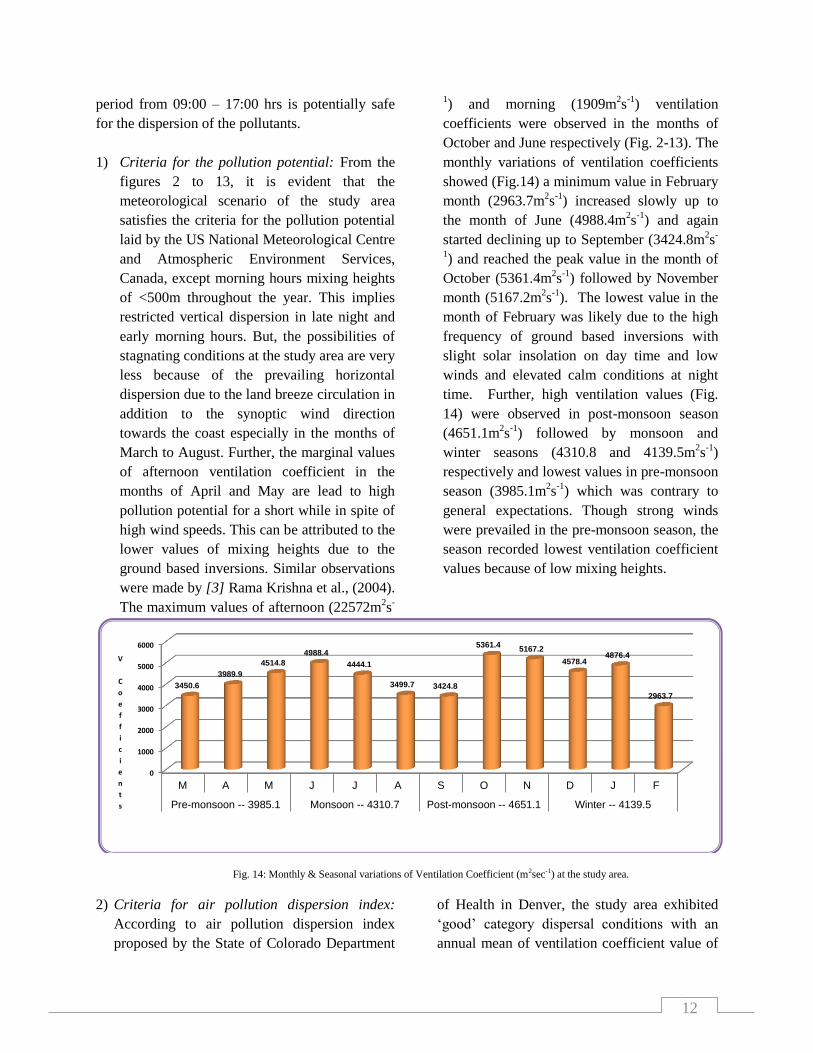
October and June respectively (Fig. 2-13). The
monthly variations of ventilation coefficients
showed (Fig.14) a minimum value in February
month (2963.7m2s
-1) increased slowly up to
the month of June (4988.4m2s
-1) and again
started declining up to September (3424.8m2s
-
1) and reached the peak value in the month of
October (5361.4m2s
-1) followed by November
month (5167.2m2s
-1). The lowest value in the
month of February was likely due to the high
frequency of ground based inversions with
slight solar insolation on day time and low
winds and elevated calm conditions at night
time. Further, high ventilation values (Fig.
14) were observed in post-monsoon season
(4651.1m2s
-1) followed by monsoon and
winter seasons (4310.8 and 4139.5m2s
-1)
respectively and lowest values in pre-monsoon
season (3985.1m2s
-1) which was contrary to
general expectations. Though strong winds
were prevailed in the pre-monsoon season, the
season recorded lowest ventilation coefficient
values because of low mixing heights.
Fig. 14: Monthly & Seasonal variations of Ventilation Coefficient (m2sec-1) at the study area.
2) Criteria for air pollution dispersion index:
According to air pollution dispersion index
proposed by the State of Colorado Department
of Health in Denver, the study area exhibited
‘good’ category dispersal conditions with an
annual mean of ventilation coefficient value of
0
1000
2000
3000
4000
5000
6000
M A M J J A S O N D J F
Pre-monsoon -- 3985.1 Monsoon -- 4310.7 Post-monsoon -- 4651.1 Winter -- 4139.5
3450.6
3989.9
4514.8
4988.4
4444.1
3499.7 3424.8
5361.4 5167.2
4578.4 4876.4
2963.7
V
C
o
e
f
f
i
c
i
e
n
t
s

13
4271.6m2s
-1 and except pre-monsoon season
(‘fair’), rest of the seasons were categorized as
‘good’ dispersal conditions (Fig. 14). But the
seasonal frequency of occurrence of hourly
dispersal/ventilation conditions was showing
different trends (Fig. 15). The maximum ‘poor’
dispersal conditions were observed in post-
monsoon and winter seasons (61.1%) followed
by monsoon season (48.6%) and a minimum of
34.7% was observed in pre-monsoon season.
‘Good’ (23.6%) and ‘fair’ (20.9%) conditions
were dominated in the pre-monsoon season
compared to other seasons (Fig. 15). ‘Poor’
dispersal conditions are very less in the month
of May (16.7%) when compared with the other
months. The extreme conditions of ‘excellent’
and ‘poor’ (Fig. 15) categorization at the study
area (except in pre-monsoon season) were
corroborated the changes of abrupt coastal
meteorological features at the study area.
Fig. 15: Seasonal and annual frequency of hourly dispersal conditions at the study area.
F. Comparison of ambient air quality (IND-AQI)
indices with ventilation coefficient based air
pollution dispersion index
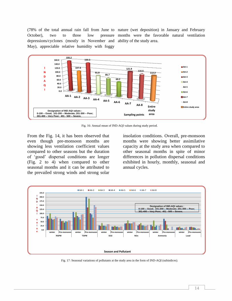
Even though, the study area exhibited annual
frequency of 51.4% ‘Poor' dispersal conditions but
it has been observed that ambient air quality on the
basis of IND-AQI scale category, the study area has
fallen under ‘moderate’ category with the annual
mean value of 112.2 (Fig. 16). The results revealed
that the seasonal mean of air quality index values
were varied from 60.2 to 143.3 and 82.8 to 226.5 in
winter and pre-monsoon seasons respectively. This
can be well compared with the ventilation
coefficient values of winter (4139.5m2s
-1) and pre-
monsoon (3985.1m2s
-1) of the present study.
Further, gaseous pollutants and RSPM were found
to be higher in winter season whereas TSPM is high
in pre-monsoon season (Fig.17). According to
present study, this can be attributed to the ground
based inversions in winter and strong winds and
low mixing heights in pre-monsoon season. The
ambient air quality at the study area was ‘moderate’
according to IND-AQI (Fig. 16) whereas the
dispersal conditions at the study area were ‘poor’
according to the air pollution dispersion index (Fig.
15). This anomaly might be due to the
topographical and the meteorological parameters of
the study area which ultimately leading to better
diffusion of pollutants. In addition to the sea/land
breeze regimes of coastal area, favorable wind
directions towards coast (most of the time from
WSW followed by W and SW), two spells of rain
fall during the southwest and northeast monsoons
0.0
10.0
20.0
30.0
40.0
50.0
60.0
70.0
Pre monsoonMonsoon
Post monsoonWinter
Annual
34
.7
48
.6
61
.1
61
.1
51
.4
20
.9
13
.9
2.8
4.2
10
.5
23
.6
8.3
6.9
5.6
11
.1
20
.8
29
.2
29
.2
29
.2
27
.1
P
e
r
c
e
n
t
a
g
e
(
%)
POOR
FAIR
GOOD
EXCELLENT
14
(78% of the total annual rain fall from June to
October), two to three low pressure
depressions/cyclones (mostly in November and
May), appreciable relative humidity with foggy
nature (wet deposition) in January and February
months were the favorable natural ventilation
ability of the study area.
Fig. 16: Annual mean of IND-AQI values during study period.
From the Fig. 14, it has been observed that
even though pre-monsoon months are
showing less ventilation coefficient values
compared to other seasons but the duration
of ‘good’ dispersal conditions are longer
(Fig. 2 to 4) when compared to other
seasonal months and it can be attributed to
the prevailed strong winds and strong solar
insolation conditions. Overall, pre-monsoon
months were showing better assimilative
capacity at the study area when compared to
other seasonal months in spite of minor
differences in pollution dispersal conditions
exhibited in hourly, monthly, seasonal and
annual cycles.
Fig. 17: Seasonal variations of pollutants at the study area in the form of IND-AQI (subindices).
0.0
20.0
40.0
60.0
80.0
100.0
120.0
140.0
160.0
AA-1 AA-2 AA-3 AA-4 AA-5 AA-6 AA-7 AA-8Entirestudyarea
155.2
107.6
150.3
91.8 85.7
69.2
121.8 116.6
112.2
I
N
D
A
Q
I
Sampling points
AA-1
AA-2
AA-3
AA-4
AA-5
AA-6
AA-7
AA-8
Entire study area
Designation of IND-AQI values : 0-100 -- Good; 101-200 -- Moderate; 201-300 -- Poor; 301-400 -- Very Poor; 401 - 500 -- Severe.
0.0
25.0
50.0
75.0
100.0
125.0
150.0
175.0
200.0
225.0
winter Pre-monsoon winter Pre-monsoon winter Pre-monsoon winter Pre-monsoon winter Pre-monsoon winter Pre-monsoon
RSPM TSPM SO2 NOx Ammonia Lead
I
N
D
-
A
Q
I
v
a
l
u
e
Season and Pollutant
AA-1 AA-2 AA-3 AA-4 AA-5 AA-6 AA-7 AA-8
Designation of IND-AQI values : 0-100 -- Good; 101-200 -- Moderate; 201-300 -- Poor; 301-400 -- Very Poor; 401 - 500 -- Severe.

International Journal of Scientific Research in Science, Engineering and Technology (ijsrset.com)
15
IV. CONCLUSION AND RECOMMENDATIONS
From the above study, it can be concluded that the
assimilative capacity of air environment of the
study area was good with natural ventilation ability
and without any stagnation of pollutants except
during early morning hours. It is recommended to
initiate necessary steps/strategies to prevent the
release and exposure of emissions during risk hours.
V. REFERENCES
[1] Prashant Gargava. 1996. Industrial Emissions in a
Coastal region of India: Prediction of Impact on Air
Environment. Environment International. 27(3), 361-
367.
[2] Pramila Goyal., Anand, S., and B.S. Gera. 2006.
Assimilative capacity and pollutant dispersion studies
for Gangtok city. Atmospheric Environment. 40, 1671-
1682. Doi:10.1016/j.atmosenv.2005.10.057.
[3] Rama Krishna, T.V.B.P.S., M.K. Reddy., R.C. Reddy
and R.N. Singh. 2004. Assimilative capacity and
dispersion of pollutants due to industrial sources in
Visakhapatnam bowl area. Atmospheric Environment.
38, 6775-6787.
[4] NEERI, 2003. Ambient air survey and air quality
management plan for Visakhapatnam bowl area.
National Environmental Engineering Research
Institute. Nagpur. India.
[5] Padmanabha Murthy, B. 2004. Environmental
Meteorology. I.K. International Pvt. Ltd., New Delhi.
[6] Edward Gross. 1970. The National Air Pollution
Potential Forecast Program. Technical Note: 70-9.
Environmental Technical Applications Center.
Washington. D.C. pp.12-13.
[7] Stalkpole, J.D., 1967. The Air Pollution Potential
Forecast Programme. ESSa Tech., Memo. WBTM-
NMC 43. [8] Deniz Derya Genc., Canan Yesilyurt., Banu Bayar and
Gurdal tuncel. 2005. Effects Of Meteorology On
Ankara Air Quality. Proceedings of the Third
International Symposium on Air Quality Management
at Urban, Regional and Global Scales. 26-30 September
2005, Istanbul – Turkey.
[9] Eagleman, J.R. 1991. Air pollution meteorlogy.
Kansas: Trimedia.
[10] Goyal, S.K. and C.V. Chalapati Rao. 2006. Air
assimilatie capacity-based environment friendly siting
of new industries - a case study of Kochi region, India.
Elsevier Ltd., doi:10.1016/j.jenvman.2006.06.020.