Discrete Volume‐Element Method for Network …cse.ucdenver.edu/~cscialtman/CVData/S_1993_C.pdf ·...

D I S C R E T E V O L U M E - E L E M E N T M E T H O D FOR N E T W O R K W A T E R - Q U A L I T Y M O D E L S

By Lewis A. Rossman, ~ Member, ASCE, Paul F. Boulos, 2 Associate Member, ASCE, and Tom Airman ~

ABSTRACT: An explicit dynamic water-quality modeling algorithm is developed for tracking dissolved substances in water-distribution networks. The algorithm is based on a mass-balance relation within pipes that considers both advective transport and reaction kinetics. Complete mixing of material is assumed at pipe junctions and storage tanks. The algorithm automatically selects a pipe-segmentation scheme and computational time step that satisfies conservation of mass and seeks to min- imize numerical dispersion. In contrast to previous water-quality models, there is no need to first find unique flow paths through the network. The resulting method is both robust and efficient, and can be readily applied to all types of network configurations and dynamic hydraulic conditions. The applicability of the method is demonstrated using an example pipe-distribution network. Enhancement of distribution-system water-quality management is a principal benefit of the methodology.

INTRODUCTION

There is currently an increasing concern on the part of water utilities and regulatory agencies regarding potential water-quality problems in drinking- water-distribution systems, Whereas considerable effort has been invested on finished water as it leaves the treatment plant, the problem of water- quality variability within the distribution system has received considerably less attention. This situation is unfortunate, since the quality of treated water (even after disinfection) may deteriorate through complex physical, chemical, and biological transformations that occur during its travel through the distribution system. Examples of such transformations include supply sources going on and off line, contamination via cross connections, system component failure, mixing of waters from sources of dissimilar quality, loss of disinfectant residual in storage facilities with long residence times, bac- terial regrowth and other microbial activities, increase in turbidity, disso- lution of lead, corrosion of pipes, and the formation of disinfection by- products, some of which are suspected carcinogens. Examples of the latter are halogenated and brominated compounds, the most publicized of which are the trihalomethanes.

Recent and pending changes in the U.S. Environmental Protection Agency (USEPA) drinking-water regulations under the Safe Drinking Water Act (SDWA) establish maximum contaminant levels (MCL) or action levels for a number of critical water-quality parameters associated with adverse health

~Chf., Engrg. and Cost Section, Drinking Water Res. Div., U.S. Envir. Protection Agency, Cincinnati, OH 45268.

2Sr. Engr., Dept. of Computer Aided Engrg., Montgomery-Watson, Pasadena, CA 91101.

3Asst. Prof., Dept. of Computer Sci. and Engrg., Univ. of Colorado, Denver, CO 80217.

Note. Discussion open until February 1, 1994. To extend the closing date one month, a written request must be filed with the ASCE Manager of Journals. The manuscript for this paper was submitted for review and possible publication on August 6, 1992. This paper is part of the Journal of Water Resources Planning and Management, Vol. 119, No. 5, September/October, 1993. �9 ISSN 0733-9496/ 93/0005-0505/$1.00 + $. 15 per page. Paper No. 4558.

505

J. Water Resour. Plann. Manage. 1993.119:505-517.

Dow

nloa

ded

from

asc

elib

rary

.org

by

Aur

aria

Lib

r-E

ss 0

4882

7825

on

05/2

1/15

. Cop

yrig

ht A

SCE

. For

per

sona

l use

onl

y; a

ll ri

ghts

res

erve

d.

effects. These regulations promulgate monitoring requirements as well as MCLs and will apply primarily to public water-supply systems of which 201,242 water systems in the continental U.S. meet this definition (Clark eta]. 1991). The current standard for trihalomethanes, the treatment-tech- nique regulations for dissolved lead and copper, the anticipated disinfection/ disinfection by-products rule, and the requirement for maintaining a chlorine residual under the Surface Water Treatment Rule (SWTR) are examples of these regulations. Exceeding MCLs or action levels requires corrective actions to be taken by water utilities. The corrective actions may include the implementation of specified treatment techniques, replacement of lead service lines, looping of dead-end mains, more frequent exercising of storage tanks, and others.

Although not presently required, the effective use of mathematical water- quality models would offer a number of benefits to the waterworks industry. Such models would have possible applications in predicting water-quality- degradation problems, calibrating system hydraulics, designing water-quality-sampling programs, optimizing the disinfection processes, evaluating the water-quality aspects of distribution-network and storage-reservoir improve- ment projects, and assessing alternative operational and control strategies for maintaining and improving water quality in distribution systems. The economic implications of the use of water-quality mathematical models are also obvious. Potential cost savings could be realized by using models to aid in optimally locating booster disinfection stations, thereby reducing the total consumption of disinfectant and, inter alia, the total disinfectant cost. Furthermore, such models could be used to plan the design of new systems or the repair and rehabilitation of existing systems prior to construction, thereby avoiding costly mistakes. This brief enumeration of possible applications, although not intended as a complete listing, does indicate the wide scope and usefulness of water-quality models.

Computer-based mathematical models are emerging as an effective means of evaluating water-quality changes in water-distribution systems (Grayman and Clark 1990, 1991). The various algorithms developed have used both steady-state and dynamic model formulations. Steady-state models determine the movement of constituents along with their travel paths and travel times throughout the distribution system under a given set of operating and loading conditions. A set of linear algebraic equations is used to describe mass conservation of the constituents at the network nodes. The nodal concentrations may be obtained using an iterative solution of the constituent nodal equations (Chun and Selznick 1985; Murphy 1985; Wood and Orms- bee 1989), sparse matrix routines (Males et al. 1985; Boulos et al. 1992), an explicit marching-out solution scheme (Clark et al. 1988a), or an explicit graph-theoretical single-step substitution process (Boulos et al. 1991; Boulos and Altman 1991). Dynamic models track the movement and transformation of constituents under time-varying conditions as the demands and other factors within the distribution-system change. The other factors include changes in storage tank levels, valve settings, storage tanks and pumps going on or off line, and rapid demand changes (fire demands). The substance- advection process is simulated numerically using the Lagrangian transport model (Liou and Kroon 1987) or the marching-out solution scheme (Clark et al. 1986, 1988b; Grayman et al. 1988; Itoh et al. 1990). Both numerical advection schemes have some similarities; however, the marching-out methodology is more easily applied to complex networks in addition to lending itself to better physical interpretation. These algorithms are predicated on

506


Dow

nloa

ded

from

asc

elib

rary

.org

by

Aur

aria

Lib

r-E

ss 0

4882

7825

on

05/2

1/15

. Cop

yrig

ht A

SCE

. For

per

sona

l use

onl

y; a

ll ri

ghts

res

erve

d.

the assumptions of one-dimensional motion, single or consecutive steady- state (extended period simulation) network flow hydraulics, complete nodal mixing, ideal plug flow with negligible dispersion, and single constituent with one or more feed sources. Typically, contaminants are treated as conservative (nonreactive and nondegradable) or as simple first-order kinetic characteristic functions. An excellent review of the various approaches was provided by Grayman and Clark (1990, 1991). However, there still remains a need for a more efficient and direct approach.

This paper presents an explicit time-driven water-quality-modeling algorithm for tracking transient concentrations of substances in pipe networks. The method is explicit in the sense that the calculation of concentrations at a given time can be directly obtained from the previously known concentration front. The substance transport phenomenon is simulated directly within the modeling process, wherein substance mass is allocated to discrete volume elements within each pipe, and within each time step, reactions occur within each element, mass is transported between elements, and mass and flow volumes are mixed together at downstream nodes. Because of the sequence in which these steps are carried out, there is no need to first identify unique flow paths of water through the network. That is, topological sorting of the network is not required.

The proposed algorithm is referred to herein as the discrete volume- element method (DVEM). A one-dimensional transport model with instantaneous complete cross-sectional mixing is assumed. Longitudinal dispersion is neglected. The algorithm is predicated on a mass-balance equation that accounts for both advective transport and reaction kinetics. Input to the model consists of a topological description of the network, a description of how hydraulic conditions in the network change over time, a reaction- rate expression for the constituent of concern, an initial distribution of the constituent throughout the network, and a description of constituent concentrations entering the network through external source flows over time. The model output produces a time history of constituent concentration at each node of the network. The solution algorithm is both robust and efficient, and can be readily applied to all types of network configurations, including natural channels, canal systems, and storm sewers. The accuracy and efficiency of the method are demonstrated using an example water- distribution network.

METHODOLOGY

Network Definition A distribution network comprises a finite number of oriented, one-di-

mensional links (pipes or channels) interconnected by nodes in some specified branched or looped configuration. Links may contain pumps (or any hydraulic component whose differential head versus flow characteristic is known, e.g., turbine and heat exchanger) and fittings, such as bends, meters, and valves, where the dissipation of concentrated energy occurs. Each link is of defined length, geometry, roughness, and material. The endpoints of each link are junction or fixed grade nodes. A junction node is a point of intersecting links and it can also be a point of external consumption where flow can enter or exit the network. A fixed grade node is a point of known energy grade such as a connection to a well, a treatment plant, a reservoir, an elevated storage facility, or a constant pressure region.

507


Dow

nloa

ded

from

asc

elib

rary

.org

by

Aur

aria

Lib

r-E

ss 0

4882

7825

on

05/2

1/15

. Cop

yrig

ht A

SCE

. For

per

sona

l use

onl

y; a

ll ri

ghts

res

erve

d.

NETWORK-FLOW PROBLEM

The transport of dissolved substances in a distribution network is closely linked to the magnitude and direction of water flow throughout the network over time. For dilute mixtures, substance-concentration levels will not affect a system's hydraulic state. One can therefore determine ahead of time how network flows will vary as external conditions change, and use these flows as inputs to a model that tracks the fate of dissolved substances. Changes in water-consumption rates, valve settings, storage tank levels, and pump operation will cause flows to change in magnitude and possibly direction. Transient flow solutions for looped, pressurized pipe networks can be found by extended period simulation (Rao et al. 1977; Bhave 1988). This involves solving a sequence of steady-state-flow problems, using methods as de- scribed in Jeppson (1981) and Osiadacz (1987), over a series of discrete time steps, where external conditions change at each time step. If greater accuracy is required, methods based on rigid water-column theory for slow transients (Onizuka 1986; Wood et al. 1989), or on elastic-water-column theory for rapid transients (Bosserman 1978; Boulos et al. 1989) can be applied. For branched, open-channel networks, transient flow conditions can be determined from numerical solutions to the shallow water-wave equations or their approximations [see Keefer and Jobson (1978), for example]. In either case, a sequence of hydraulic states for the network between fixed hydraulic time steps can be found to serve as inputs to a water-quality model.

CONSTITUENT TRANSPORT PROBLEM

Analytical Formulation During a hydraulic time step, all flow and velocity patterns remain con-

stant. Within this step, the concentration within link i, Ci(x, t), at any point x (in the positive flow direction) and time t is given by solutions to the mass- conservation differential equation

_ _ aC~(x , t) oCi(x , t) ~- U i - R[Ci (x , t ) ] = 0 . . . . . . . . . . . . . . . . . . . . . . . . (1) Ot Ox

where ui = mean flow velocity of the water; and R[C~(x, t)] -- a reaction- rate expression. For example, the reaction-rate expression most commonly used is a first-order rate function of the form

R(C,) = cr . . . . . . . . . . . . . . . . . . . . . . . . . . . . . . . . . . . . . . . . . . . . . . . . ( 2 )

where oL denotes a coefficient of concentration decay (negative) or growth (positive) rate. This coefficient is zero for conservative substances. The closed-form solution to (1) may then be written as

X C , ( x , t + "0 = C , ( x - u, ,~, Oe~'~; v , ~ <- - . . . . . . . . . . . . . . . . . . . . . ( 3 )

Ui

which implies that any distribution of substance concentration within link i at time t is advected a distance uF in time interval T under an exponential kinetic concentration change. The time interval T is referred to as the water- quality time step. We present this closed-form solution for example purposes only. Our DVEM approach is capable of handling more-complicated reaction schemes that do not have closed-form solutions.

Concentrations at the link endpoints are determined from mass conservation of the constituent itself. Complete and instantaneous nodal mixing

508


Dow

nloa

ded

from

asc

elib

rary

.org

by

Aur

aria

Lib

r-E

ss 0

4882

7825

on

05/2

1/15

. Cop

yrig

ht A

SCE

. For

per

sona

l use

onl

y; a

ll ri

ghts

res

erve

d.

is assumed. The boundary condition at a junction node k (with a negligible detention time) for each outgoing link i may be expressed as

13k

QjCj(Lj, t)

c,(o, t ) = c~(t) J ~ = ~ . . . . . . . . . . . . . . . . . . . . . . . . . . . . . (4)

j~.{k}

where C~ denotes the constituent concentration at junction node k; {k} = set of incoming links at junction node k; ~k = cardina]ity of {k}; Qi = volumetric flow rate in link j; and Lj = its length. The boundary condition at a variable-level storage tank with an incoming link i may be expressed a s

1 Cr(t + ~) - Vy( t ) + Qi~ [Ci(Li, t)Q~7 + V~(t)Cy(t)] . . . . . . . . . . . . . (5)

while an outgoing link j carries the fully mixed tank concentration, i.e.

Cj(0, t + r) = Cr(t ) . . . . . . . . . . . . . . . . . . . . . . . . . . . . . . . . . . . . . . . . . (6)

where CT and VT = fully mixed concentration and volume of the tank, respectively. Eq. (6) also applies to all fixed grade nodes with constant water volume. It is possible to relax the assumption of complete mixing within tanks if some other mixing model applies, such as a multicompartment mixing model (Grayman et al. 1991).

Because the concentration profile along any of the network links is a function of upstream concentrations, the analytical solution to this problem becomes intractable for all but the simplest network arrangements. As a result, a robust and efficient, yet numerically explicit, method is developed.

Numerical Scheme The discrete volume-element method (DVEM) is predicated on a fun-

damental plug flow substance mass balance that accounts for advective transport and kinetic reaction processes, wherein substance mass is assigned to discrete volume elements within each link, reactions occur within each element, substance mass is advected from one element to the next, and mass and flow volumes are mixed together at the network nodes.

Each link in the network is divided into a number of equal sized elements spaced evenly along the link axis. Let vi denote the volume of the elements in link i and m# the mass within each element. Over a water-quality time step 7, mass is advected between adjacent elements while also undergoing a kinetic reaction change. To ensure that water is not transported beyond its downstream boundary node, a link's volume element must be chosen to be less than or equal to QiT, and �9 cannot be greater than the shortest travel time through any of the network links associated with a particular hydraulic event. That is

n i = . . . . . . . . . . . . . . . . . . . . . . . . . . . . . . . . . . . . . . . . . . . . . . . . ( 8 )

509


Dow

nloa

ded

from

asc

elib

rary

.org

by

Aur

aria

Lib

r-E

ss 0

4882

7825

on

05/2

1/15

. Cop

yrig

ht A

SCE

. For

per

sona

l use

onl

y; a

ll ri

ghts

res

erve

d.

v, v, = - - . . . . . . . . . . . . . . . . . . . . . . . . . . . . . . . . . . . . . . . . . . . . . . . . . . . . (9)

ni

where Vi = total volume of link i (length of link multiplied by its cross- sectional area); ~li = number of volume elements in link i; and the floor function La/designates the largest integer less than or equal to a.

When all of the network links have been partitioned into volume elements and the initial mass distribution computed, the propagation of mass through the network over each water-quality time step proceeds in four phases: a kinetic reaction step, in which the mass in each volume element undergoes a kinetic concentration change; a nodal mixing step, in which mass and volume are mixed together at nodes; an advective step, in which mass is moved between adjacent volume elements; and an allocation step, in which nodal mass is attached to the first (head) volume element of all outgoing links. These steps are illustrated in Fig. 1 and are summarized in the following.

Step 1: React the mass within each volume element over the water-quality time interval "r to arrive at new mass rn~ k. For a first-order kinetic reaction

rn; ~ = m ~ e ~ ; i = 1 . . . . , L and k = 1 . . . . . "qi . . . . . . . . . . . . (10)

where L = number of links. Step 2: Transport mass and flow volume from the last (tail) element of

each link into its connecting node and compute a new nodal concentration, i.e.

M]= s m~ TM

iE{ j }

6]

"17/ = ~ ei.r ie{j}

. . . . . . . . . . . . . . . . . . . . . . . . . . . . . . . . . . . . . . . . . . . . . ( 1 1 )

. . . . . . . . . . . . . . . . . . . . . . . . . . . . . . . . . . . . . . . . . . . . . . ( 1 2 )

Original Mass

After Reaction

Transport Into Node

Transport Along Link

Transport Out of Node

FIG. 1. Mass-Transport Steps within Link

510


Dow

nloa

ded

from

asc

elib

rary

.org

by

Aur

aria

Lib

r-E

ss 0

4882

7825

on

05/2

1/15

. Cop

yrig

ht A

SCE

. For

per

sona

l use

onl

y; a

ll ri

ghts

res

erve

d.

Cj -- Mj . . . . . . . . . . . . . . . . . . . . . . . . . . . . . . . . . . . . . . . . . . . . . . . . . . . (13) Vj

where Mj = mass entering node j; m~ ~i = reacted mass in the tail volume element of link i; Vj = total volume entering node j; and Cj = concentration at node j.

Step 3: Shift mass from volume element k to k + 1 of each link, i.e.

m~ k+l = m~k; i = 1 , . . . , N a n d k = 1 . . . . . ~1i - 1 . . . . . . . . (14)

Step 4: Move mass out of each node into the first volume element of all outgoing links, i.e.

m ; ' = C j Q s ' r . . . . . . . . . . . . . . . . . . . . . . . . . . . . . . . . . . . . . . . . . . . . . . (15)

where link i has flow out of node j. The computer program to implement this scheme proceeds as follows.

One pass is made through the collection of network links, reacting substance mass within each volume element and transferring the resulting mass to the next downstream element. For the last element in the link, the mass and corresponding flow volume are accumulated at the node connected to the element. Then a pass is made through each node of the network, using the accumulated masses and flow volumes to compute nodal concentrations. Finally, a second pass is made through the network links, moving mass out of the head node of each link into its first volume element.

This sequence is repeated for each water-quality time step T until the next hydraulic event takes place. At the very last time step, �9 may have to be reduced so that the total elapsed time will just equal the hydraulic time step associated with the particular event. In this case, the mass advected from one volume element to another is adjusted by the ratio of T'/~, where ~' is the reduced water-quality time step. Calculations are terminated when all hydraulic events have been considered. Observe that the sequencing of these steps precludes the need to determine a priori a water-quality time step, link-segmentation scheme, or unique set of flow paths through the network.

The D V E M link-segmentation scheme can be modified to accommodate two extreme cases. Very short pipes with high velocities might cause ~ to assume a very small value, thus leading to excessive computation times. In practice, this can be avoided by specifying a minimum allowable water- quality time step Xmi.. Pipes with smaller travel times will experience a delay in mass transport through them, causing some loss of accuracy in the solutions obtained. Nonpipe components in the system, such as pumps or valves, can be assumed to have instantaneous transport of mass across them without any sacrifice in accuracy. A second extreme occurs for very long pipes with slow velocities. This can result in a very large number of segments in the pipe and again slow down the computations or cause computer memory to be exceeded. In this case a maximum number of segments, -q . . . . can be imposed. Pipes requiring more than this number of segments will cause mass to be transported faster than it actually should.

Constituent Mass Distribution In our numerical scheme, the constituent mass distribution needs to be

represented along the network links at the start of the simulation and at the start of each hydraulic event when the sizes of the elements may change due to changes in velocity and/or flow direction. At the start of the simulation, constituent concentrations at the network nodes are provided as

511


Dow

nloa

ded

from

asc

elib

rary

.org

by

Aur

aria

Lib

r-E

ss 0

4882

7825

on

05/2

1/15

. Cop

yrig

ht A

SCE

. For

per

sona

l use

onl

y; a

ll ri

ghts

res

erve

d.

initial conditions. Observed concentrations or concentrations obtained from a steady-state model may be used (Grayman et al. 1988). After a link is segmented into volume elements for the first hydraulic time step, the edge element masses are determined using a linear interpolation of the concentrations at the two distinct end nodes as follows:

mk i = COy, + (k - 1)(C~ i - - C~ (~q,-- 1) , k = 1 , . . . , ~qi

and i = 1 , . . . , E . . . . . . . . . . . . . . . . . . . . . . . . . . . . . . . . . . . . . . . . . . (16)

where C O and C?i = concentrations at the head and tail ends of the link i, respectively. For links with a single element (~li = 1)

m ) - (C~ + C~)v~ (17) . . . . . . . . . . . . . . . . . . . . . . . . . . . . . . . . . . . . . . . . . .

The occurrence of a new hydraulic event induces a change in the link segmentation. As a result, the constituent mass distribution within each link needs to be redefined. This can be done by overlaying the old segmentation and its mass distribution over the new one. Two cases are possible. First, the new segmentation possesses fewer elements than the old one. In this case, mass and volume from each old element are directly transferred to a new element until the new element volume is full. The next new element is then considered. When it only takes a portion of the old element volume to fill a new element, a proportional amount of the old element is transferred to the new element. The remainder goes to the next new element. Second, the new segmentation comprises more elements. In this case, a volume equal to the new element and to each successive new element is transferred from an old element, with a proport ional amount of mass, until the old

From More to Fewer Segments

From Fewer to More Segments

FIG. 2. Redistribution of Mass within Link

512


Dow

nloa

ded

from

asc

elib

rary

.org

by

Aur

aria

Lib

r-E

ss 0

4882

7825

on

05/2

1/15

. Cop

yrig

ht A

SCE

. For

per

sona

l use

onl

y; a

ll ri

ghts

res

erve

d.

@

@

63.1 m3/sec

3/sec

Symbols

[ - ~ ~ = 50,5 m3/sec ([.._~[_._] Junction Node Link

O Fixed Grade Node

FIG. 3. Example Distribution Network

TABLE 1. Link Characteristics

Rough- Link Head Tail Length Diameter ness Flow Velocity

number node node (m) (mm) coefficien! (m3/s) (m/s) (1) (2) (3) (4) (5) (6) (7) (8)

1 A 1 610 203 120 59.1 1.82 2 1 2 732 152 120 6.35 0.348 3 C 2 305 203 120 62.0 1.91 4 3 2 1,220 152 120 7.44 0.409 5 3 1 366 152 120 10.3 0.564 6 B 3 671 203 120 68.3 2.10

TABLE 2. Junction-Node Characteristics

Junction Elevation Demand Grade Pressure number (m) (m3/s) (m) (kPa)

(1) (2) (3) (4) (5)

1 24.4 63,1 70.9 455 2 36.6 75.8 70.0 327 3 25.9 50.5 72.0 451

element is depleted. Fig. 2 i l lustrates the two cases of redis t r ibut ing constituent mass within a link at the start of a new hydraulic event. Observe that when the direct ion of flow in a link changes be tween hydraulic events, the distr ibution of mass within that link is explicit ly computed in reverse order. That is, the mass f rom the l ink 's first old e lement is t ransferred to the last new e lement first, and so on. These redistr ibui tons of mass can be made one link at a t ime; there is no need to keep two comple te link segmentat ions for the ent ire ne twork in memory at the same time.

513


Dow

nloa

ded

from

asc

elib

rary

.org

by

Aur

aria

Lib

r-E

ss 0

4882

7825

on

05/2

1/15

. Cop

yrig

ht A

SCE

. For

per

sona

l use

onl

y; a

ll ri

ghts

res

erve

d.

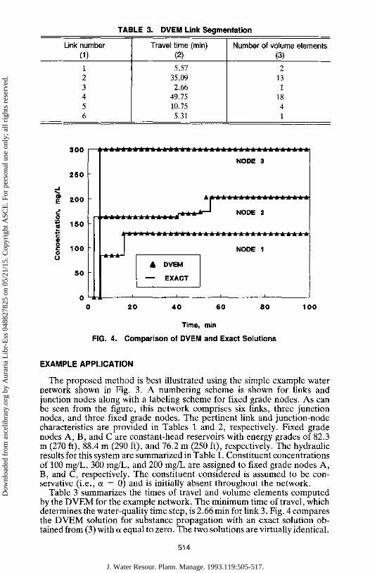
TABLE 3. DVEM Link Segmentat ion

Link number Travel time (min) Number of volume elements (1) (2) (3)

5.57 35.09 2.66

49.75 10.75 5.31

2 13 1

18 4 1

, . I ?. E

0

t

0 0

0

3 0 0

2 5 0

2 0 0

1 5 0

1 0 0

5 0

NODE 3

- r - �9 " " ~ NODE 2

. . . . . . . . . . . . . . . . . . . . . . . . . . . .~ .ik . t ,L .L "r

. . . / NODE 1

m m 0 I I I

0 2 0 6 0 8 0 1 0 0

�9 DVEM

EXACT

I

4 0

Time, rain

FIG. 4. Compar ison of DVEM and Exact Solutions

E X A M P L E A P P L I C A T I O N

The proposed method is best illustrated using the simple example water network shown in Fig. 3. A numbering scheme is shown for links and junction nodes along with a labeling scheme for fixed grade nodes. As can be seen from the figure, this network comprises six links, three junction nodes, and three fixed grade nodes. The pertinent link and junction-node characteristics are provided in Tables 1 and 2, respectively. Fixed grade nodes A, B, and C are constant-head reservoirs with energy grades of 82.3 m (270 fl), 88.4 m (290 ft), and 76.2 m (250 fl), respectively. The hydraulic results for this system are summarized in Table 1. Constituent concentrations of 100 rag/L, 300 rag/L, and 200 mg/L are assigned to fixed grade nodes A, B, and C, respectively. The constituent considered is assumed to be conservative (i.e., ot = 0) and is initially absent throughout the network.

Table 3 summarizes the times of travel and volume elements computed by the DVEM for the example network. The minimum time of travel, which determines the water-quality time step, is 2.66 rain for link 3. Fig. 4 compares the DVEM solution for substance propagation with an exact solution obtained from (3) with c~ equal to zero. The two solutions are virtually identical.

514


Dow

nloa

ded

from

asc

elib

rary

.org

by

Aur

aria

Lib

r-E

ss 0

4882

7825

on

05/2

1/15

. Cop

yrig

ht A

SCE

. For

per

sona

l use

onl

y; a

ll ri

ghts

res

erve

d.

CONCLUSIONS

An explicit dynamic water-quality modeling algorithm has been pre- sented. It possesses a number of advantages over the current state-of-the- art methods, including automatic selection of pipe segmentation and computational time step, decreased memory and computational requirements, and elimination of the need for topological sorting.

The proposed method allows for efficient simulation of the spatial and temporal distribution of substances in water networks. Because of an increasing concern regarding potential water-quality problems in pipe-distribution networks, the method promises to have broad practical applications. The message is clear. Water-quality assessment, monitoring, and control in distribution systems have become key issues in practically every hydraulic engineering endeavor.

The DVEM provides a simple and flexible, yet very effective, tool for enhancing engineering insight into the dynamics of water-quality variations and complex processes that take place in pipe-distribution systems. The method is general and can be readily applied to piping systems conveying fluid other than water as a commodity.

Because the DVEM is predicated directly on system hydraulics, increased importance should be attached to defining realistic hydraulic models with particular emphases on correct system skeletonization, calibration and hydraulic event characteristics, along with a proper definition of constituent kinetic characteristics. Poorly defined models may result in poor prediction of quality parameters and thus defeat the whole purpose of the water-quality- modeling-process. In any case, since all mass-balance relationships are sat- isfied, the proposed method will always yield mathematically consistent water-quality parameter solutions.

ACKNOWLEDGMENT

This material is based upon work partially funded by the U.S. Environ- mental Protection Agency and the American Water Works Research Foun- dation. It has not been subject to the agency's review and therefore does not necessarily reflect the views of the agency, and no official endorsement should be inferred. The support received is gratefully acknowledged.

APPENDIXI. REFERENCES

Bhave, P. R. (1988). "Extended period simulation of water systems--direct solution." J. Envir. Engrg., ASCE, 114(5), 1146-1159.

Bosserman, B. E. (1978). "Computer analysis of hydraulic transients in a complex piping system." J. Am. Water Works Assoc., 70, 371-376.

Boulos, P. F., and Altman, T. (1991). "Improved algorithms for modeling water quality in complex pipe distribution systems." Computer Sci. and Engrg. Tech. Rep. 9-1991, University of Colorado, Denver, Colo.

Boulos, P. F., Wood, D. J., and Funk, J. E. (1989). "A comparison of numerical and exact solutions for pressure surge analysis." Proc., 6th Int. Conf. on Pressure Surges, A. R. D. Thorley, ed., BHRA, Cambridge, England, 149-159.

Boulos, P. F., Altman, T., and Sadhal, K. (1992). "Computer modeling of water quality in large multiple source networks." J. Appl. Math. Modeling, 16(8), 439- 445.

Boulos, P. F., Altman, T., and Vasconcelos, J. J. (1991). "Explicit graph-theoretic algorithms for mixing problems in multiple-source networks." Computer Sci. and Engrg. Tech. Rep. 4-1991, University of Colorado, Denver, Colo.

515


Dow

nloa

ded

from

asc

elib

rary

.org

by

Aur

aria

Lib

r-E

ss 0

4882

7825

on

05/2

1/15

. Cop

yrig

ht A

SCE

. For

per

sona

l use

onl

y; a

ll ri

ghts

res

erve

d.

(;hun, D. G., and Selznick, H. L. (1985). "Computer modeling of distribution system water quality." Computer applications in water resources, ASCE, New York, N.Y.

Clark, R. M., Grayman, W. M., Males, R. M., and Coyle, J. M. (1986). "Predicting water quality in distribution systems." Proc., Distribution System Syrup., AWYqA, Minneapolis, Minn.

Clark, R. M., Grayman, W. M., and Males, R. M. (1988a). "Contaminant propagation in distribution systems." J. Envir. Engrg., ASCE, 114(4), 929-943.

Clark, R. M., Grayman, W. M., Males, R. M., and Coyle, J. M. (1988b). "Modeling contaminant propagation in drinking water distribution systems." AQUA, 3, 137- 151.

Clark, R. M., Grayman, W. M., and Goodrich, J. A. (1991). "Water quality modeling: its regulatory implications." Proc., A WWARFIEPA Conf. on Water Quality Modeling in Distribution Systems, Cincinnati, Ohio.

Grayman, W. M., Clark, R. M., and Males, R. M. (1988), "Modeling distribution system water quality: dynamic approach." J. Water Resour. Plng. and Mgmt., ASCE, 114(3), 295-312.

Grayman, W. M., and Clark, R. M. (1990). "An overview of water quality modeling in a distribution system." Proc., 1990 A W W A Annu. Conf., Cincinnati, Ohio.

Grayman, W. M., and Clark, R. M. (1991). "Water quality modeling in distribution systems." Syrup. on Dynamics of Water Quality in Distribution Systems, A WWA Annu. Conf., Philadelphia, Pa.

Grayman, W. M., Clark, R. M., and Goodrich, J. A. (1991). "The effects of operation, design, and location of storage tanks on the water quality in a distribution system." Proe. , A WWARF/EPA Conf. on Water Quality Modeling in Distribution Systems, Cincinnati, Ohio.

ltoh, H., Kurotani, K., Kubota, M., and Tsuzura, M. (1990). "Dynamic analysis concerning water quality in distribution networks and advanced control for chlorine injection." Proc., IAWPR Conf., Kyoto, Japan.

Jeppson, R. W. (1981). Analysis of flow in pipe networks. Ann Arbor Science, Ann Arbor, Mich.

Keefer, T. N., and Jobson, H. E. (1978). "River transport modeling for unsteady flows." J. Hydr. Div., ASCE, 104(5), 635-647.

Liou, C. P., and Kroon, J. R. (1987). "Modeling the propagation of waterborne substances in distribution networks." J. Am. Water Works Assoc., 79(11), 54-58.

Males, R. M., Clark, R. M., Wehrman, P. J., and Gates, W. E. (1985). "Algorithm for mixing problems in water systems." J. Hydr. Engrg., ASCE, 111(2), 206-219.

Murphy, S. B. (1985). "Modeling chlorine concentrations in municipal water systems," MS. thesis, Montana State University, Bozeman, Mont.

Onizuka, K. (1986). "System dynamics approach to pipe network analysis." J. Hydr. Engrg., ASCE 112(8), 728-749.

Osiadacz, A. J. (1987). Simulation and analysis of gas networks. E&F Spon Ltd., London, England.

Rao, H. S., and Bree, D. W. (1977). "Extended period simulation of water systems-- part A." J. Hydr. Div., ASCE, 103(2), 97-108.

Wood, D. J., and Ormsbee, L. E. (1989). "Supply identification for water distribution systems." J. Am. Water Works Assoc., 81(7), 74-80.

Wood, D. J., Funk, J. E., and Boulos, P. F. (1989). "Pipe network transients-- distributed and lumped parameter modeling." Proc., 6th Int. Conf. on Pressure Surges, A. R. D. Thorley, ed., BURA, Cambridge, England, 131-142.

A P P E N D I X II. N O T A T I O N

The following symbols are used in this paper:

C = concentration (ML-3); N = number of links in network;

{k} = set of incoming links at node; L = link length (L);

516


Dow

nloa

ded

from

asc

elib

rary

.org

by

Aur

aria

Lib

r-E

ss 0

4882

7825

on

05/2

1/15

. Cop

yrig

ht A

SCE

. For

per

sona

l use

onl

y; a

ll ri

ghts

res

erve

d.

M = total mass en te r ing n o d e (M); m k = mass in e l e m e n t k (M); Q = vo lumet r ic flow rate (L3T-1) ; R = reac t ion rate ( M L - 3 T - 1 ) ;

t = t ime (T); u = flow veloci ty ( L T - 1 ) ; V = total v o l u m e of flow en te r ing node (L3);

Vr = t ank v o l u m e (L3); x = dis tance (L);

= f i rs t -order reac t ion rate cons tan t ( T - l ) ; 13k = cardinal i ty of set {k}; r I = n u m b e r of v o l u m e e l emen t s in l ink; v = vo lume of e l e m e n t (L3); and -r = t ime in terva l (T).

Subscr ip ts i, j = l inks;

k = j unc t i on node ; and T = tank.

517


Dow

nloa

ded

from

asc

elib

rary

.org

by

Aur

aria

Lib

r-E

ss 0

4882

7825

on

05/2

1/15

. Cop

yrig

ht A

SCE

. For

per

sona

l use

onl

y; a

ll ri

ghts

res

erve

d.

Discrete Volume‐Element Method for Network …cse.ucdenver.edu/~cscialtman/CVData/S_1993_C.pdf ·...

Documents

Transcript of Discrete Volume‐Element Method for Network …cse.ucdenver.edu/~cscialtman/CVData/S_1993_C.pdf ·...