Discrete Principal Component Analysis?

Wray Buntine1 and Aleks Jakulin2

1 Complex Systems Computation Group (CoSCo),Helsinki Institute for Information Technology (HIIT)

P.O. Box 9800, FIN-02015 HUT, Finland.Wray.Buntine@hiit.fi

2 Department of Knowledge TechnologiesJozef Stefan Institute

Jamova 39, 1000 Ljubljana, Sloveniajakulin@gmail.com

Abstract. This article presents a unified theory for analysis of com-ponents in discrete data, and compares the methods with techniquessuch as independent component analysis (ICA), non-negative matrixfactorisation (NMF) and latent Dirichlet allocation (LDA). The mainfamilies of algorithms discussed are mean field, Gibbs sampling, andRao-Blackwellised Gibbs sampling. Applications are presented for votingrecords from the United States Senate for 2003, and the use of compo-nents in subsequent classification.

1 Introduction

Principal component analysis (PCA), latent semantic indexing (LSI), and inde-pendent component analysis (ICA, see [19]) are key methods in the statisticalengineering toolbox. They have a long history, are used in many different ways,and under different names. They were primarily developed in the engineeringcommunity where the notion of a filter is common, and maximum likelihoodmethods less so. They are usually applied to measurements and real valueddata, and used for feature extraction or data summarization.

Relatively recently the statistical computing community has become aware ofseemingly similar approaches for discrete data that appears under many names:grade of membership (GOM) [31], probabilistic latent semantic indexing (PLSI)[17], non-negative matrix factorisation (NMF) [23], genotype inference using ad-mixtures [29], latent Dirichlet allocation (LDA) [5], multinomial PCA (MPCA)[6], multiple aspect modelling [26], and Gamma-Poisson models (GaP) [9]. Werefer to these methods jointly as Discrete PCA (DPCA), and this article providesa unifying model for them. Note also, that it is possible these methods existedin reduced form in other statistical fields perhaps decades earlier.

These methods are applied in the social sciences, demographics and med-ical informatics, genotype inference, text and image analysis, and information

? Draft paper for the PASCAL Bohinj workshop. Cite as HIIT Technical Report, July2005.

retrieval. By far the largest body of applied work in this area (using citationindexes) is in genotype inference due to the Structure program [29]. A grow-ing body of work is in text classification and topic modelling (see [16, 8]), andlanguage modelling in information retrieval (see [1, 7, 9]).

Here we present in Section 3 a unified theory for analysis of components in dis-crete data, and compare the methods with related techniques. The main familiesof algorithms discussed are mean field, Gibbs sampling, and Rao-BlackwellisedGibbs sampling in Section 5. Applications are presented in Section 6 for votingrecords from the United States Senate for 2003, and the use of components insubsequent classification.

2 Views of DPCA

One interpretation of the DPCA methods is that they are a way of approximatinglarge sparse discrete matrices. Suppose we have a 500, 000 documents made upof 1, 500, 000 different words. A document such as a page out of Dr. Zeuss’s The

Cat in The Hat, is first given as a sequence of words.

So, as fast as I could, I went after my net. And I said, “With my net Ican bet them I bet, I bet, with my net, I can get those Things yet!”

It can be put in the bag of words representation, where word order is lost, as alist of words and their counts in brackets:

so (1) as (2) fast (1) I (7) could (1) went (1) after (1) my (3) net (3) and(1) said (1) with (2) can (2) bet (3) them (1) get (1) those (1) things (1)yet (1) .

This sparse vector can be represented as a vector in full word space with 1, 499, 981zeroes and the counts above making the non-zero entries in the appropriateplaces. Given a matrix made up of rows of such vectors of non-negative integersdominated by zeros, it is called here a large sparse discrete matrix.

Bag of words is a basic representation in information retrieval [2]. The al-ternative is sequence of words. In DPCA, either representation can be used andthe models act the same, up to any word order effects introduced by incrementalalgorithms. This detail is made precise in subsequent sections.

In this section, we argue from various perspectives that large sparse discretedata is not well suited to standard PCA, which is implicitly Gaussian, or ICAmethods, which are justified using continuous data.

2.1 DPCA as Approximation

In the PCA method, one seeks to approximate a large matrix by a productof smaller matrices, by eliminating the lower-order eigenvectors, the least con-tributing components in the least squares sense. This is represented in Figure 1.If there are I documents, J words and K components, then the matrix on the

(a)

docu

ments

words

(b)

words

docu

ments

components

Fig. 1. The Matrix View: matrix product (b) approximates sparse discrete matrix (a)

left has I ∗ J entries and the two matrices on the right have (I + J) ∗K entries.This represents a simplification when K � I, J . We can view DPCA methodsas seeking the same goal in the case where the matrices are sparse and discrete.

When applying PCA to large sparse discrete matrices, interpretation becomesdifficult. Negative values appear in the component matrices, so they cannot beinterpreted as “typical documents” in any usual sense. This applies to many otherkinds of sparse discrete data: low intensity images (such as astronomical images)and verb-noun data used in language models introduced by [27], for instance.DPCA, then, places constraints on the approximating matrices in Figure 1(b)so that they are also non-negative.

Also, there are fundamentally two different kinds of large sample approximat-ing distributions that dominate discrete statistics: the Poisson and the Gaussian.For instance, a large sample binomial is approximated as a Poisson when theprobability is small and as a Gaussian otherwise [30]. Thus in image analysisbased on analogue to digital converters, where data is counts, Gaussian errorscan sometimes be assumed, but the Poisson should be used if counts are small.DPCA then avoids Gaussian modelling of the data.

2.2 Independent Components

Independent component analysis (ICA) was also developed as an alternativeto PCA. Hyvanen and Oja [20] argue that PCA methods merely decorrelatedata, finding uncorrelated components. ICA then was developed as a way ofrepresenting multivariate data with truly independent components. The basicformulation is that a K-dimensional data vector w is a linear function of K in-dependent components represented as aK-dimensional hidden vector l, w = Θl

for square matrix Θ. For some univariate density function g(), the independentcomponents are distributed as p(l) =

∏k g(lk). This implies

p(w |Θ) =∏

k

g ((Θw)k)1

det(Θ)

The Fast ICA algorithm [20] can be interpreted as a maximum likelihood ap-proach based on this probability formula. In the sparse discrete case, however,

this formulation breaks down for the simple reason that w is mostly zeros: theequation can only hold if l and Θ are discrete as well and thus the gradient-based algorithms for ICA cannot be justified. To get around this in practice,when applying ICA to documents [4], word counts are sometimes first turnedinto TF-IDF scores [2].

To arrive at a formulation more suited to discrete data, we can relax theequality in ICA (i.e., w = Θl) to be an expectation:

Expp(w|l) (w) = Θl .

We still have independent components, but a more general relationship thenexists with the data. Correspondence between ICA and DPCA has been reportedin [7, 9]. Note with this expectation relationship, the dimension of l can now beless than the dimension of w, and thus Θ would be a rectangular matrix.

For p(w |Θ) in the so-called exponential family distributions [15], the ex-pected value of w is referred to as the dual parameter, and it is usually theparameter we know best. For the Bernoulli with probability p, the dual parame-ter is p, for the Poisson with rate λ, the dual parameter is λ, and for the Gaussianwith mean µ, the dual parameter is the mean. Our formulation, then, can be alsobe interpreted as letting w be exponential family with dual parameter given by(Θl). Our formulation then generalises PCA in the same way that linear models[25] generalises linear regression3.

Note, an alternative has also been presented [13] where w has an exponentialfamily distribution with natural parameters given by (Θl). For the Bernoulli withprobability p, the natural parameter is log p/(1 − p), for the Poisson with rateλ, the natural parameter is logλ and for the Gaussian with mean µ, the naturalparameter is the mean. This formulation generalises PCA in the same way thatgeneralised linear models [25] generalises linear regression.

3 The Basic Model

A good introduction to these models from a number of viewpoints is by [5, 9, 7].Here we present a general model and show its relationship to previous work. Thenotation of words, bags and documents will be used throughout, even thoughother kinds of data representations also apply. In machine learning terminology,a word is a feature, a bag is a data vector, and a document is a sample. Noticethat the bag collects the words in the document and loses their ordering. The bagis represented as a data vector w. It is now J-dimensional, and the hidden vectorl called the components is K-dimensional, where K < J . The term component

is used here instead of, for instance, topic. The parameter matrix Θ is J ×K.

3.1 Bags or Sequences of Words?

For a document d represented as a sequence of words, if w = bag(d) is its baggedform, the bag of words, represented as a vector of counts, then for any modelM

3 Though it is an artifact of statistical methods in general that linear models are bestdefined as generalised linear models with a linear link function.

that consistently handles both kinds of data

p(w |M) =(∑wj)!∏

j wj !p(d |M) . (1)

Note that some likelihood based methods such as maximum likelihood, someBayesian methods, and some other fitting methods (for instance, a cross valida-tion technique) use the likelihood as a functional. They take values or derivativesbut otherwise do not further interact with the likelihood. The combinatoric firstterm on the right hand side of Equation (1) can be dropped here safely becauseit does not affect the fitting of the parameters for M. Thus for these methods,it is irrelevant whether the data is treated as a bag or as a sequence. This is ageneral property of multinomial data.

Some advanced fitting methods such as Gibbs sampling do not treat thelikelihood as a functional. They introduce hidden variables that changes thelikelihood, and they may update parts of a document in turn. For these, orderingaffects can be incurred by bagging a document, since updates for different partsof the data will now be done in a different order. But the combinatoric firstdata dependent term in Equation (1) will still be ignored and the algorithmsare effectively the same up to the ordering affects. Thus, while we consider bag

of words in this article, all the theory equally applies to the sequence of words

representation. Implementation can easily address both cases with little change

to the algorithms, just to the data handling routines.

3.2 General DPCA

The general formulation introduced in Section 2.2 is an unsupervised version ofa linear model, and it applies to the bag of words w (the sequence of wordsversion replaces w with d) as

w ∼ PDD(Θl,α1) such that Expp(w|l) (w) = Θl (2)

l ∼ PDC(α2) ,

where PDD(·, ·) is a discrete vector valued probability distribution, PDC(·) is acontinuous vector valued probability density function that may introduce con-straints on the domain of l such as non-negativity. The hyper-parameter vectorsα1 and α2 might also be in use. In the simplest case these two distributions area product of univariate distributions, so we might have lk ∼ PDc(αk) for each kas in Section 2.2.

Various cases of DPCA can now be represented in terms of this format, asgiven in Table 1. The discrete distribution is the multivariate form of a binomialwhere an index j ∈ {0, 1, ..., J − 1} is selected according to a J-dimensionalprobability vector. A multinomial with total count L is the bagged version of Ldiscretes. In the table, non-spec indicates that this aspect of the model was leftunspecified. Note that NMF used a cost function formulation, and thus avoideddefining likelihood models. PLSI used a weighted likelihood formulation thattreated hidden variables without defining a distribution for them.

Table 1. DPCA Example Models

Name Bagged PDD PDC Constraints

NMF [23] yes non-spec non-spec lk ≥ 0PLSI [17] no discrete non-spec lk ≥ 0,

∑k

lk = 1LDA [5] no discrete Dirichlet lk ≥ 0,

∑k

lk = 1MPCA [6] yes multinomial Dirichlet lk ≥ 0,

∑k

lk = 1GaP [9] yes Poisson gamma lk ≥ 0

The formulation of Equation (2) is also called an admixture in the statisticalliterature [29]. Let θk be the k-th row of Θ. The parameters for the distributionof w are formed by making a weighted sum of the parameters represented bythe K vectors θk. This is in contrast with a mixture model [15] which is formedby making a weighted sum of the probability distributions PDD(θk,α1).

3.3 The Gamma-Poisson Model

The general Gamma-Poisson form of DPCA, introduced as GaP [9] is now con-sidered in more detail:

– Document data is supplied in the form of word counts. The word count foreach word type is wj . Let L be the total count, so L =

∑j wj .

– The document also has hidden component variables lk that indicate theamount of the component in the document. In the general case, the lk areindependent and gamma distributed

lk ∼ Gamma(αk , βk) for k = 1, . . . ,K.

The βk affects scaling of the components4, while αk changes the shape ofthe distribution.

– Initially the K-dimensional hyper-parameter vectors α and β will be treatedas constants, and their estimation will be considered later.

– There is a general model matrix Θ of size J×K with entries θj,k that controlsthe partition of features amongst each component. This is normalised alongrows (

∑j .θj,k = 1).

– The data is now Poisson distributed, for each j

wj ∼ Poisson((Θl)j) .

The hidden or latent variables here are the vector l. The model parameters arethe gamma hyper-parameters β and α, and the matrix Θ. The full likelihoodfor each document then becomes:

∏

k

βαk

k lαk−1k e−βklk

Γ (αk)

∏

j

(∑

k lkθj,k)wj e−(∑

klkθj,k)

wj !(3)

4 Note conventions for the gamma vary. Sometimes a parameter 1/βk is used. Ourconvention is revealed in Equation (3).

To obtain a full posterior for the problem, these terms are multiplied across alldocuments, and a Dirichlet prior for Θ added in.

3.4 The Dirichlet-Multinomial Model

The Dirichlet-multinomial form of DPCA was introduced as MPCA. In this case,the normalised hidden variables m are used, and the total word count L is notmodelled.

m ∼ DirichletK(α) , w ∼ Multinomial(Θm, L)

The full likelihood for each document then becomes:

CLwΓ

(∑

k

αk

)∏

k

mαk−1k

Γ (αk)

∏

j

(∑

k

lkθj,k

)wj

(4)

where CLw is L choose w. LDA has the multinomial replaced by a discrete, and

thus the choose term drops, as per Section 3.1. PLSI is related to LDA butlacks a prior distribution on m. It does not model these hidden variables usingprobability theory, but instead using a weighted likelihood method [17].

4 Aspects of the Model

Before starting analysis and presenting algorithms, this section discusses someuseful aspects of the DPCA model family.

4.1 Correspondence

While it was argued in Section 3.4 that LDA and MPCA are essentially the samemodel, up to ordering effects5 it is also the case that these methods have a closerelationship to GaP.

Consider the Gamma-Poisson model. A set of Poisson variables can alwaysbe converted into a total Poisson and a multinomial over the set [30]. The set ofPoisson distributions on wj then is equivalent to:

L ∼ Poisson

(∑

k

lk

), w ∼ Multinomial

(1∑k lk

Θl, L

).

Moreover, if the β hyper-parameter is a constant vector, then mk = lk/∑

k lk isdistributed as a Dirichlet, DirichletK(α), and

∑k lk is distributed independently

as a gamma Γ (∑

k αk, β). The second distribution above can then be representedas

w ∼ Multinomial (Θm, L) .

Note also, that marginalising out∑

k lk convolves a Poisson and a gamma distri-bution to produce a Poisson-Gamma distribution for L [3]. Thus, we have proventhe following.

5 Note that the algorithm for MPCA borrowed the techniques of LDA directly.

Lemma 1. Given a Gamma-Poisson model of Section 3.3 where the β hyper-

parameter is a constant vector with all entries the same, β, the model is equiva-

lent to a Dirichlet-multinomial model of Section 3.4 where mk = lk/∑

k lk, and

in addition

L ∼ Poisson-Gamma

(∑

k

αk, β, 1

)

The implication is that if α is treated as known, and not estimated from thedata, then L is aposteriori independent of m and Θ. In this context, when theβ hyper-parameter is a constant vector, LDA, MPCA and GaP are equivalentmodels ignoring representational issues. If α is estimated from the data in GaP,then the presence of the data L will influence α, and thus the other estimatessuch as of Θ. In this case, LDA and MPCA will no longer be effectively equivalentto GaP. Note, Canny recommends fixing α and estimating β from the data [9].

To complete the set of correspondences, note that in Section 5.1 it is proventhat NMF corresponds to a maximum likelihood version of GaP, and thus it alsocorresponds to a maximum likelihood version of LDA, MPCA, and PLSI. Torelationship is made by normalising the matrices that result.

4.2 A Multivariate Version

Another variation of the methods is to allow grouping of the count data. Wordscan be grouped into separate variable sets. These groups might be “title words,”“body words,” and “topics” in web page analysis or “nouns,” “verbs” and “ad-jectives” in text analysis. The groups can be treated with separate discrete dis-tributions, as below. The J possible word types in a document are partitionedinto G groups B1, . . . , BG. The total word counts for each group g is denotedLg =

∑j∈Bg

wj . If the vector w is split up into G vectors wg = {wj : j ∈ Bg},

and the matrix Θ is now normalised by group in each row, so∑

j∈Bgθj,k = 1,

then a multivariate version of MPCA is created so that for each group g,

wg ∼ Multinomial

({∑

k

mkθj,k : j ∈ Bg

}, Lg

).

Fitting and modelling methods for this variation are related to LDA or MPCA,and will not be considered in more detail here. This has the advantage thatdifferent kinds of words have their own multinomial and the distribution of dif-ferent kinds is ignored. This version is demonstrated subsequently on US Senatevoting records, where each multinomial is now a single vote.

4.3 Component Assignments for Words

In standard mixture models, each document in a collection is assigned to one(hidden) component. In the DPCA family of models, each word in each docu-ment is assigned to one (hidden) component. To see this, we introduce anotherhidden vector which represents the component assignments for different words.

As in Section 3.1, this can be done using a bag of components or a sequence ofcomponents representation, and no effective change occurs in the basic models,or in the algorithms so derived. What this does is expand out the term Θl intoparts, treating it as if it is the result of marginalising out some hidden variable.Here we just treat the two cases of Gamma-Poisson and Dirichlet-multinomial.

We introduce a K-dimensional discrete hidden vector c whose total countis L, the same as the word count. This records the component for each wordin a bag of components representation. Thus ck gives the number of words inthe document appearing in the k-th component. Its posterior mean makes anexcellent diagnostic and interpretable result. A document from the sports newsmight have 50 “football” words, 10 “German” words, 20 “sports fan” words and20 “general vocabulary” words. So an estimate or expected value for v·,k is thusused to give the amount of a component in a document, and forms the basis ofany posterior analysis and hand inspection of the results.

With the new hidden vector, the distributions underlying the Gamma-Poissonmodel become:

lk ∼ Gamma(αk , βk) (5)

ck ∼ Poisson (lk)

wj =∑

k

vj,k where vj,k ∼ Multinomial (θk, ck) .

The joint likelihood thus becomes, after some rearrangement

∏

k

βαk

k lck+αk−1k e−(βk+1)lk

Γ (αk)

∏

j,k

θvj,k

j,k

vj,k!. (6)

Note that l can be marginalised out, yielding

∏

k

Γ (ck + αk)

Γ (αk)

βαk

k

(βk + 1)ck+αk

∏

j,k

θvj,k

j,k

vj,k!(7)

and the posterior mean of lk given c is (ck + αk)/(1 + βk). Thus each ck ∼Poisson-Gamma(αk, βk, 1). For the Dirichlet-multinomial model, a similar re-construction applies:

m ∼ DirichletK(α) (8)

ck ∼ Multinomial (m, L)

wj =∑

k

vj,k where vj,k ∼ Multinomial (θk, ck) .

The joint likelihood thus becomes, after some rearrangement

L!Γ

(∑

k

αk

)∏

k

mck+αk−1k

Γ (αk)

∏

j,k

θvj,k

j,k

vj,k !. (9)

Again, m can be marginalised out yielding

L!Γ (∑

k αk)

Γ (L+∑

k αk)

∏

k

Γ (ck + αk)

Γ (αk)

∏

j,k

θvj,k

j,k

vj,k !. (10)

Note, in both the Gamma-Poisson and Dirichlet-multinomial models each countwj is the sum of counts in the individual components, wj =

∑k vj,k . The sparse

matrix vj,k of size J ×K is thus a hidden variable, with row totals wj given inthe data and column totals ck.

4.4 Historical Notes

The first clear enunciation of the large-scale model in its Poisson form comes from[23], and in its multinomial form from [17] and [29]. The first clear expressionof the problem as a hidden variable problem is given by [29], although no doubtearlier versions appear in statistical journals under other names, and perhapsin reduced dimensions (e.g., K = 3). The application of Gibbs is due to [29],and of the mean field method is due to [5], the newer fast Gibbs version to [16].The mean field method was a significant introduction because of its speed. Therelationship between LDA and PLSI and that NMF was a Poisson version ofLDA was first pointed out by [6]. The connections to ICA come from [7] and[9]. The general Gamma-Poisson formulation, perhaps the final generalisation tothis line of work, is in [9].

5 Algorithms

Neither of the likelihoods yield to standard EM analysis. For instance, in thelikelihood Equation (6) and (9), the hidden variables l/m and v/c are coupled,which is not compatible with the standard EM theory. Most authors point outthat EM-like analysis applies and use EM terminology, and indeed this is thebasis of the mean field approach for this problem. For the exponential family,mean field algorithms correspond to an extension of the EM algorithm [6]. EMand maximum likelihood algorithms can be used if one is willing to include thehidden variables in the optimization criterion, as done for instance with theK-means algorithm.

Algorithms for this problem follow some general approaches in the statisticalcomputing community:

– Straight maximum likelihood such as by [23], sometimes expressed as aKullback-Leibler divergence,

– annealed maximum likelihood by [17], best viewed in terms of its clusteringprecursor such as by [18],

– Gibbs sampling on v, l/m and Θ in turn using a full probability distributionby [29], or Gibbs sampling on v alone (or equivalently, component assign-ments for words in the sequence of words representation) after marginalisingout l/m and Θ by [16],

– mean field methods by [5], and

– expectation propagation (like so-called cavity methods) by [26].

The maximum likelihood algorithms are not considered here. Their use is al-ways discouraged when a large number of hidden variables exist, and they aremostly simplifications of the algorithms here,. Expectation propagation does notscale, thus it is not considered subsequently either. While other algorithms typ-ically require O(L) or O(K) hidden variables stored per document, expectationpropagation requires O(KL).

To complete the specification of the problem, a prior is needed for Θ. ADirichlet prior can be used for each k-th component of Θ with J prior parametersγj , so θk ∼ DirichletJ (γ).

5.1 Mean Field

The mean field method was first applied to the sequential variant of the Dirichlet-multinomial version of the problem by [5]. In the mean field approach, generallya factored posterior approximation q() is developed for the hidden variables l

(or m) and v, and it works well if it takes the same functional form as theprior probabilities for the hidden variables. The functional form of the approx-imation can be derived by inspection of the recursive functional forms (see [6]Equation (4)):

q(l)←→1

Zl

exp(Eq(v) {log p (l,v,w |Θ,α,β,K)}

)(11)

q(v) ←→1

Zv

exp(Eq(l) {log p (l,v,w |Θ,α,β,K)}

),

where the Zl and Zr are normalising constants.

An important computation used during convergence in this approach is alower bound on the individual document log probabilities, log p (w |Θ,α,β,K).This comes naturally out of the mean field algorithm (see [6] Equation (6)).Using the approximation q() defined by the above distributions, the bound isgiven by

Expq() (log p (l,v,w |Θ,α,β,K)) + I(q()) . (12)

The mean field algorithm applies to the Gamma-Poisson version and the Dirichlet-multinomial version.

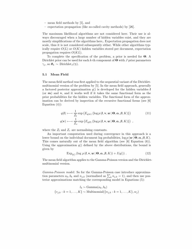
Gamma-Poisson model: So for the Gamma-Poisson case introduce approxima-tion parameters ak, bk and nj,k (normalised as

∑k nj,k = 1), and then use pos-

terior approximations matching the corresponding model in Equations (5):

lk ∼ Gamma(ak, bk)

{vj,k : k = 1, . . . ,K} ∼ Multinomial({nj,k : k = 1, . . . ,K}, wj)

for each document. Matching the likelihood these two form with Equation (6),according to the rules of Equations (11), yields the re-write rules for these newparameters:

nj,k =1

Zj

θj,k exp(log lk

), (13)

ak = αk +∑

j

wjnj,k ,

bk = 1 + βk ,

where log lk ≡ Explk | ak .bk(log lk) = Ψ0(ak)− log bk ,

Zj ≡∑

k

θj,k exp(log lk

).

Here, Ψ0() is the digamma function. These equations form the first step of eachmajor cycle, and are performed on each document.

The second step is to re-estimate the original model parameters Θ using theposterior approximation by maximising the expectation according to q(l,v) ofthe log of the full posterior probability Expq() (log p (l,v,w,Θ, |α,β,K)). Thisincorporates Equation (6) for each document, and a Dirichlet prior term forΘ. Denote the intermediate variables n for the i-th document by adding a (i)subscript, as nj,k,(i), and likewise for wj,(i). All these log probability formulasyield linear terms in θj,k, thus one gets

θj,k ∝∑

i

wj,(i)nj,k,(i) + γj . (14)

The lower bound on the log probability of Equation (12), after some simplifica-tion and use of the rewrites of Equation (13), becomes

log1∏

j wj !+∑

k

((αk − ak) log lk − log

Γ (αk)bak

k

Γ (ak)βαk

k

)+∑

j

wj logZj . (15)

The mean field algorithm for Gamma-Poisson version is given in Figure 2.

Dirichlet-multinomial model: For the Dirichlet-multinomial case, the mean fieldalgorithm takes a related form. The approximate posterior is given by:

m ∼ Dirichlet(a)

{vj,k : k = 1, . . . ,K} ∼ multinomial({nj,k : k = 1, . . . ,K}, wj)

This yields the same style update equations as Equations (13) except that βk = 1

nj,k =1

Zj

θj,k exp(logmk

), (16)

ak = αk +∑

j

wjnj,k ,

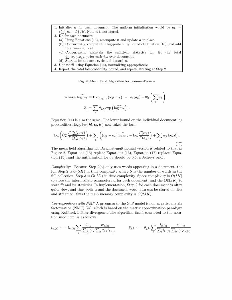
1. Initialise a for each document. The uniform initialisation would be ak =(∑k

αk + L)

/K. Note n is not stored.2. Do for each document:

(a) Using Equations (13), recompute n and update a in place.(b) Concurrently, compute the log-probability bound of Equation (15), and add

to a running total.(c) Concurrently, maintain the sufficient statistics for Θ, the total∑

iwj,(i)nj,k,(i) for each j, k over documents.

(d) Store a for the next cycle and discard n.3. Update Θ using Equation (14), normalising appropriately.4. Report the total log-probability bound, and repeat, starting at Step 2.

Fig. 2. Mean Field Algorithm for Gamma-Poisson

where logmk ≡ Expmk |a(log mk) = Ψ0(ak)− Ψ0

(∑

k

ak

),

Zj ≡∑

k

θj,k exp(logmk

).

Equation (14) is also the same. The lower bound on the individual document logprobabilities, log p (w |Θ,α,K) now takes the form

log

(CL

w

Γ (∑

k αk)

Γ (∑

k ak)

)+∑

k

((αk − ak) logmk − log

Γ (αk)

Γ (ak)

)+∑

j

wj logZj .

(17)The mean field algorithm for Dirichlet-multinomial version is related to that inFigure 2. Equations (16) replace Equations (13), Equation (17) replaces Equa-tion (15), and the initialisation for ak should be 0.5, a Jeffreys prior.

Complexity: Because Step 2(a) only uses words appearing in a document, thefull Step 2 is O(SK) in time complexity where S is the number of words in thefull collection. Step 3 is O(JK) in time complexity. Space complexity is O(IK)to store the intermediate parameters a for each document, and the O(2JK) tostore Θ and its statistics. In implementation, Step 2 for each document is oftenquite slow, and thus both a and the document word data can be stored on diskand streamed, thus the main memory complexity is O(2JK).

Correspondence with NMF A precursor to the GaP model is non-negative matrixfactorisation (NMF) [24], which is based on the matrix approximation paradigmusing Kullback-Leibler divergence. The algorithm itself, converted to the nota-tion used here, is as follows

lk,(i) ←− lk,(i)

∑

j

θj,k∑j θj,k

wj,(i)∑k θj,klk,(i)

θj,k ←− θj,k

∑

i

lk,(i)∑i lk,(i)

wj,(i)∑k θj,klk,(i)

Notice that the solution is indeterminate up to a factor ψk. Multiple lk,(i) by ψk

and divide θj,k by ψk and the solution still holds. Thus, without loss of generality,let θj,k be normalised on j, so that

∑j θj,k = 1.

Lemma 2. Take a solution to the NMF equations, and divide θj,k by a factor

ψk =∑

j θj,k, and multiply lk,(i) by the same factor. This is equivalent to a

solution for the following rewrite rules

lk,(i) ←− lk,(i)

∑

j

θj,k

wj,(i)∑k θj,klk,(i)

θj,k ∝ θj,k

∑

i

lk,(i)

wj,(i)∑k θj,klk,(i)

where θj,k is kept normalised on j.

Proof. First prove the forward direction. Take the scaled solution to NMF. TheNMF equation for lk,(i) is equivalent to the equation for lk,(i) in the lemma. Takethe NMF equation for θj,k and separately normalise both sides. The

∑i lk,(i) term

drops out and one is left with the equation for θj,k in the lemma. Now prove thebackward direction. It is sufficient to show that the NMF equations hold for thesolution to the rewrite rules in the lemma, since θj,k is already normalised. TheNMF equation for lk,(i) clearly holds. Assuming the rewrite rules in the lemmahold, then

θj,k =

θj,k

∑i lk,(i)

wj,(i)∑k

θj,klk,(i)∑j θj,k

∑i lk,(i)

wj,(i)∑k

θj,klk,(i)

=

θj,k

∑i lk,(i)

wj,(i)∑k

θj,klk,(i)∑i lk,(i)

∑j θj,k

wj,(i)∑k

θj,klk,(i)

(reorder sum)

=θj,k

∑i lk,(i)

wj,(i)∑k

θj,klk,(i)∑i lk,(i)

(apply first rewrite rule)

Thus the second equation for NMF holds.

The importance of this lemma is in realising that the introduced set of equationsare the maximum likelihood version of the mean-field algorithm for the Gamma-Poisson model. That is, NMF where Θ is returned normalised is a maximumw.r.t. Θ and l for the Gamma-Poisson likelihood p(w |Θ, l,α = 0,β = 0,K).This can be seen by inspection of the equations at the beginning of this sec-tion. Note, including a hidden variable such as l in the likelihood is not correctmaximum likelihood, and for clustering yields the K-means algorithm.

5.2 Gibbs Sampling

There are two styles of Gibbs sampling that apply.

Direct Gibbs sampling: The basic Prichard’s style Gibbs sampling works offEquation (6) or Equation (9) together with a Dirichlet prior for rows of Θ.The hidden variables can easily seen to be conditionally distributed in theseequations according to standard probability distributions, in a manner allowingdirect application of Gibbs sampling methods. The direct Gibbs algorithm forboth versions is given in Figure 3. This Gibbs scheme then re-estimates each

1. For each document, retrieve the last c from store, then(a) Sample the hidden component variables:

i. In the Gamma-Poisson case, lk ∼ Gamma(ck+αk, 1+βk) independently.ii. In the Dirichlet-multinomial case, l ∼ Dirichlet({ck + αk : k}).

(b) For each word j in the document with positive count wj , the componentcounts vector, from Equation (5) and Equation (8),

{vj,k : k = 1, . . . , K} ∼ Multinomial

({lkθj,k∑k

lkθj,k

: k

}, wj

).

Alternatively, if the sequence-of-components version is to be used, the compo-nent for each word can be sampled in turn using the corresponding Bernoullidistribution.

(c) Concurrently, record the log-probabilityi. In the Gamma-Poisson case, p (w | l,Θ, α, β, K).ii. In the Dirichlet-multinomial case, p (w |m, L,Θ, α, β, K).

These represent a reasonable estimate of the likelihood p (w |Θ, α, β, K).(d) Concurrently, maintain the sufficient statistics for Θ, the total∑

iwj,(i)nj,k,(i) for each j, k over documents.

(e) Store c for the next cycle and discard v.2. Using a Dirichlet prior for rows of Θ, and having accumulated all the counts v

for each document in sufficient statistics for Θ, then its posterior has rows thatare Dirichlet. Sample.

3. Report the total log-probability, and report.

Fig. 3. One Major Cycle of Gibbs Algorithm for DPCA

of the variables in turn. In implementation, this turns out to correspond to themean field algorithms, excepting that sampling is done instead of maximisationor expectation.

Rao-Blackwellised Gibbs sampling: The Griffiths-Steyvers’ style Gibbs samplingis a Rao-Blackwellisation (see [11]) of direct Gibbs sampling. It takes the likeli-hood versions of Equations (7) and (10) multiplied up for each document togetherwith a prior on Θ, and marginalises out Θ. As before, denote the hidden vari-ables v for the i-th document by adding an (i) subscript, as vj,k,(i). Then theGamma-Poisson posterior for documents i ∈ 1, . . . , I , with Θ and l marginalised,

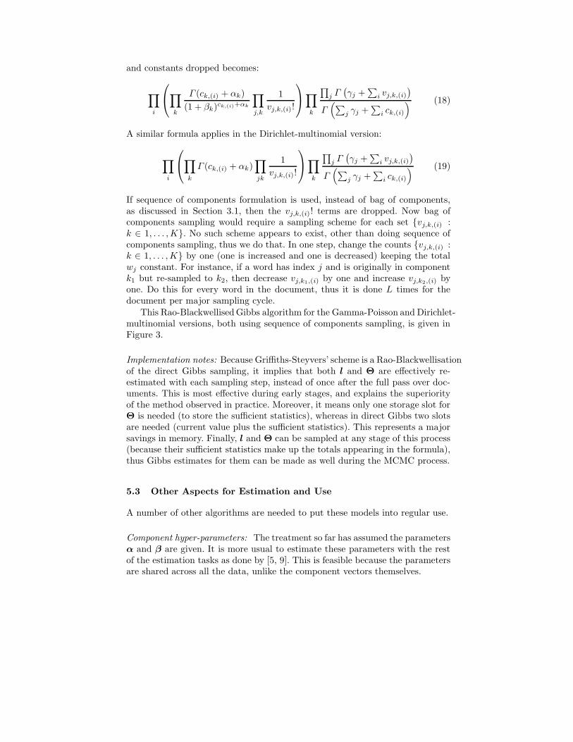
and constants dropped becomes:

∏

i

∏

k

Γ (ck,(i) + αk)

(1 + βk)ck,(i)+αk

∏

j,k

1

vj,k,(i)!

∏

k

∏j Γ(γj +

∑i vj,k,(i)

)

Γ(∑

j γj +∑

i ck,(i)

) (18)

A similar formula applies in the Dirichlet-multinomial version:

∏

i

∏

k

Γ (ck,(i) + αk)∏

jk

1

vj,k,(i)!

∏

k

∏j Γ(γj +

∑i vj,k,(i)

)

Γ(∑

j γj +∑

i ck,(i)

) (19)

If sequence of components formulation is used, instead of bag of components,as discussed in Section 3.1, then the vj,k,(i)! terms are dropped. Now bag ofcomponents sampling would require a sampling scheme for each set {vj,k,(i) :k ∈ 1, . . . ,K}. No such scheme appears to exist, other than doing sequence ofcomponents sampling, thus we do that. In one step, change the counts {vj,k,(i) :k ∈ 1, . . . ,K} by one (one is increased and one is decreased) keeping the totalwj constant. For instance, if a word has index j and is originally in componentk1 but re-sampled to k2, then decrease vj,k1,(i) by one and increase vj,k2,(i) byone. Do this for every word in the document, thus it is done L times for thedocument per major sampling cycle.

This Rao-Blackwellised Gibbs algorithm for the Gamma-Poisson and Dirichlet-multinomial versions, both using sequence of components sampling, is given inFigure 3.

Implementation notes: Because Griffiths-Steyvers’ scheme is a Rao-Blackwellisationof the direct Gibbs sampling, it implies that both l and Θ are effectively re-estimated with each sampling step, instead of once after the full pass over doc-uments. This is most effective during early stages, and explains the superiorityof the method observed in practice. Moreover, it means only one storage slot forΘ is needed (to store the sufficient statistics), whereas in direct Gibbs two slotsare needed (current value plus the sufficient statistics). This represents a majorsavings in memory. Finally, l and Θ can be sampled at any stage of this process(because their sufficient statistics make up the totals appearing in the formula),thus Gibbs estimates for them can be made as well during the MCMC process.

5.3 Other Aspects for Estimation and Use

A number of other algorithms are needed to put these models into regular use.

Component hyper-parameters: The treatment so far has assumed the parametersα and β are given. It is more usual to estimate these parameters with the restof the estimation tasks as done by [5, 9]. This is feasible because the parametersare shared across all the data, unlike the component vectors themselves.

1. Maintain the sufficient statistics for Θ, given by∑

ivj,k,(i) for each j and k, and

the individual component assignment for each word in each document.2. For each document i, retrieve the component assignments for each word then

(a) Recompute statistics for l(i) given by ck,(i) =∑

jvj,k,(i) for each k from the

individual component assignment for each word.(b) For each word in the document:

i. Re-sample the component assignment for the word according to Equa-tion (18) or (19) with the vj,k,(i)! terms dropped. If v′

j,k,(i) is the wordcounts without this word, and c′k,(i) the corresponding component totals,then this simplifies dramatically (e.g., Γ (x + 1)/Γ (x) = x).A. For the Gamma-Poisson, sample the component proportionally to

c′k,(i) + αk

1 + βk

γj +∑

iv′

j,k,(i)∑jγj +

∑ic′k,(i)

B. For the Dirichlet-multinomial, sample the component proportionallyto

(c′k,(i) + αk)γj +

∑iv′

j,k,(i)∑jγj +

∑ic′k,(i)

ii. Concurrently, record the log-probability p (w | c,Θ, α, β, K). It repre-sents a reasonable estimate of the likelihood p (w |Θ, α, β, K).

iii. Concurrently, update the statistics for l/m and Θ.

Fig. 4. One Major Cycle of Rao-Blackwellised Gibbs Algorithm for DPCA

Estimating the number of components K: A simple scheme exists within im-portance sampling in Gibbs to estimate the evidence term for a DPCA model,proposed by [7], first proposed in the general sampling context by [10]. Onewould like to find the value of K with the highest posterior probability (or, forinstance, cross validation score). In popular terms, this could be used to findthe “right” number of components, though in practice and theory such a thingmight not exist.

Use on new data: A typical use of the model requires performing inference relatedto a particular document. Suppose, for instance, one wished to estimate how wella snippet of text, a query, matches a document. Our document’s components aresummarised by the hidden variables m (or l). If the new query is representedby q, then p(q|m,Θ,K) is the matching quantity one would like ideally. Sincem is unknown, we must average over it. Various methods have been proposed[26, 7].

Alternative components: Hierarchical components have been suggested [7] asa way of organising an otherwise large flat component space. For instance,the Wikipedia with over half a million documents can easily support the dis-covery of several hundred components. Dirichlet processes have been devel-oped as an alternative to the K-dimensional component priors in the Dirichlet-

multinomial/discrete model [32], although in implementation the effect is to useK-dimensional Dirichlets for a large K and delete low performing components.

6 Applications

This section briefly discusses a two applications of the methods.

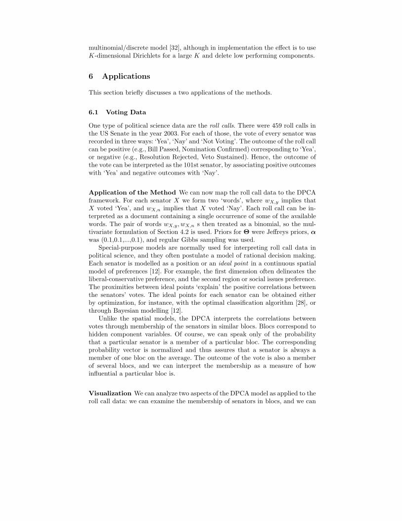
6.1 Voting Data

One type of political science data are the roll calls. There were 459 roll calls inthe US Senate in the year 2003. For each of those, the vote of every senator wasrecorded in three ways: ‘Yea’, ‘Nay’ and ‘Not Voting’. The outcome of the roll callcan be positive (e.g., Bill Passed, Nomination Confirmed) corresponding to ‘Yea’,or negative (e.g., Resolution Rejected, Veto Sustained). Hence, the outcome ofthe vote can be interpreted as the 101st senator, by associating positive outcomeswith ‘Yea’ and negative outcomes with ‘Nay’.

Application of the Method We can now map the roll call data to the DPCAframework. For each senator X we form two ‘words’, where wX,y implies thatX voted ‘Yea’, and wX,n implies that X voted ‘Nay’. Each roll call can be in-terpreted as a document containing a single occurrence of some of the availablewords. The pair of words wX,y, wX,n s then treated as a binomial, so the mul-tivariate formulation of Section 4.2 is used. Priors for Θ were Jeffreys priors, α

was (0.1,0.1,...,0.1), and regular Gibbs sampling was used.Special-purpose models are normally used for interpreting roll call data in

political science, and they often postulate a model of rational decision making.Each senator is modelled as a position or an ideal point in a continuous spatialmodel of preferences [12]. For example, the first dimension often delineates theliberal-conservative preference, and the second region or social issues preference.The proximities between ideal points ‘explain’ the positive correlations betweenthe senators’ votes. The ideal points for each senator can be obtained eitherby optimization, for instance, with the optimal classification algorithm [28], orthrough Bayesian modelling [12].

Unlike the spatial models, the DPCA interprets the correlations betweenvotes through membership of the senators in similar blocs. Blocs correspond tohidden component variables. Of course, we can speak only of the probabilitythat a particular senator is a member of a particular bloc. The correspondingprobability vector is normalized and thus assures that a senator is always amember of one bloc on the average. The outcome of the vote is also a memberof several blocs, and we can interpret the membership as a measure of howinfluential a particular bloc is.

Visualization We can analyze two aspects of the DPCA model as applied to theroll call data: we can examine the membership of senators in blocs, and we can

examine the actions of blocs for individual issues. The approach to visualizationis very similar, as we are visualizing a set of probability vectors. We can use thegray scale to mirror the probabilities ranging from 0 (white) to 1 (black).

As yet, we have not mentioned the choice of K - the number of blocs. Al-though the number of blocs can be a nuisance variable, such a model is distinctlymore difficult to show than one for a fixed K. We obtain the following negativelogarithms to the base 2 of the model’s likelihood forK = 4, 5, 6, 7, 10: 9448.6406,9245.8770, 9283.1475, 9277.0723, 9346.6973. We see that K = 5 is overwhelm-ingly selected over all others, with K = 4 being far worse. This means that withour model, we best describe the roll call votes with the existence of five blocs.Fewer blocs do not capture the nuances as well, while more blocs would not yieldreliable probability estimates given such an amount of data. Still, those modelsare too valid to some extent. It is just that for a single visualization we pick thebest individual one of them.

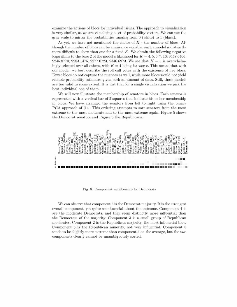
We will now illustrate the membership of senators in blocs. Each senator isrepresented with a vertical bar of 5 squares that indicate his or her membershipin blocs. We have arranged the senators from left to right using the binaryPCA approach of [14]. This ordering attempts to sort senators from the mostextreme to the most moderate and to the most extreme again. Figure 5 showsthe Democrat senators and Figure 6 the Republicans.

Box

er (D

−CA

)H

arki

n (D

−IA

)Sa

rban

es (D

−MD

)L

evin

(D−M

I)L

eahy

(D−V

T)

Ree

d (D

−RI)

Lau

tenb

erg

(D−N

J)C

linto

n (D

−NY

)D

urbi

n (D

−IL

)K

enne

dy (D

−MA

)M

ikul

ski (

D−M

D)

Cor

zine

(D−N

J)St

aben

ow (D

−MI)

Ker

ry (D

−MA

)Sc

hum

er (D

−NY

)E

dwar

ds (D

−NC

)M

urra

y (D

−WA

)G

raha

m (D

−FL

)A

kaka

(D−H

I)R

ocke

felle

r (D

−WV

)C

antw

ell (

D−W

A)

Dod

d (D

−CT

)R

eid

(D−N

V)

Byr

d (D

−WV

)D

asch

le (D

−SD

)K

ohl (

D−W

I)L

iebe

rman

(D−C

T)

John

son

(D−S

D)

Fein

gold

(D−W

I)In

ouye

(D−H

I)D

ayto

n (D

−MN

)B

inga

man

(D−N

M)

Wyd

en (D

−OR

)D

orga

n (D

−ND

)Fe

inst

ein

(D−C

A)

Nel

son

(D−F

L)

Bid

en (D

−DE

)H

ollin

gs (D

−SC

)C

onra

d (D

−ND

)Pr

yor (

D−A

R)

Jeff

ords

(I−V

T)

Bay

h (D

−IN

)C

arpe

r (D

−DE

)L

inco

ln (D

−AR

)L

andr

ieu

(D−L

A)

Bau

cus

(D−M

T)

Bre

aux

(D−L

A)

Nel

son

(D−N

E)

Out

com

eM

iller

(D−G

A)

Dem

ocra

ts

12345

Fig. 5. Component membership for Democrats

We can observe that component 5 is the Democrat majority. It is the strongestoverall component, yet quite uninfluential about the outcome. Component 4 isare the moderate Democrats, and they seem distinctly more influential thanthe Democrats of the majority. Component 3 is a small group of Republicanmoderates. Component 2 is the Republican majority, the most influential bloc.Component 5 is the Republican minority, not very influential. Component 5tends to be slightly more extreme than component 4 on the average, but the twocomponents clearly cannot be unambiguously sorted.

Cha

fee

(R−R

I)Sn

owe

(R−M

E)

Col

lins

(R−M

E)

Out

com

eM

cCai

n (R

−AZ

)Sp

ecte

r (R

−PA

)C

ampb

ell (

R−C

O)

Gre

gg (R

−NH

)Sm

ith (R

−OR

)D

eWin

e (R

−OH

)M

urko

wsk

i (R

−AK

)V

oino

vich

(R−O

H)

Hut

chis

on (R

−TX

)C

olem

an (R

−MN

)Fi

tzge

rald

(R−I

L)

Ens

ign

(R−N

V)

Stev

ens

(R−A

K)

War

ner (

R−V

A)

Lug

ar (R

−IN

)Su

nunu

(R−N

H)

Gra

ham

(R−S

C)

Hag

el (R

−NE

)B

row

nbac

k (R

−KS)

Shel

by (R

−AL

)R

ober

ts (R

−KS)

Dom

enic

i (R

−NM

)B

ond

(R−M

O)

Tal

ent (

R−M

O)

Gra

ssle

y (R

−IA

)D

ole

(R−N

C)

Sant

orum

(R−P

A)

Hat

ch (R

−UT

)B

enne

tt (R

−UT

)L

ott (

R−M

S)A

llen

(R−V

A)

Cha

mbl

iss

(R−G

A)

Bur

ns (R

−MT

)Fr

ist (

R−T

N)

Inho

fe (R

−OK

)C

ochr

an (R

−MS)

Alla

rd (R

−CO

)A

lexa

nder

(R−T

N)

McC

onne

ll (R

−KY

)Se

ssio

ns (R

−AL

)B

unni

ng (R

−KY

)C

orny

n (R

−TX

)C

rapo

(R−I

D)

Kyl

(R−A

Z)

Cra

ig (R

−ID

)E

nzi (

R−W

Y)

Nic

kles

(R−O

K)

Tho

mas

(R−W

Y)

Rep

ublic

ans

12345

Fig. 6. Component membership for Republicans

7 Classification Experiments

We tested the use of MPCA in its role as a feature construction tool, a commonuse for PCA and ICA, and as a classification tool. For this, we used the 20 news-groups collection described previously as well as the Reuters-21578 collection6.We employed the SVMlight V5.0 [22] classifier with default settings. For classi-fication, we added the class as a distinct multinomial (cf. Section 4.2) for thetraining data and left it empty for the test data, and then predicted the classvalue. Note that for performance and accuracy, SVM is the clear winner: as thestate of the art optimized discrimination-based system this is to be expected. Itis interesting to see how MPCA compares.

Each component can be seen as generating a number of words in each doc-ument. This number of component-generated words plays the same role in clas-sification as does the number of lexemes in the document in ordinary classifica-tion. In both cases, we employed the TF-IDF transformed word and component-generated word counts as feature values. Since SVM works with sparse datamatrices, we assumed that a component is not present in a document if thenumber of words that would a component have generated is less than 0.01. Thecomponents alone do not yield a classification performance that would be com-petitive with SVM, as the label has no distinguished role in the fitting. However,we may add these component-words in the default bag of words, hoping that theconjunctions of words inherent to each component will help improve the classi-fication performance.

For the Reuters collection, we used the ModApte split. For each of the 6 mostfrequent categories, we performed binary classification. Further results are dis-closed in Table 27. No major change was observed by adding 50 components tothe original set of words. By performing classification on components alone, theresults were inferior, even with a large number of components. In fact, with 300

6 The Reuters-21578, Distribution 1.0 test collection is available from David D. Lewis’professional home page, currently: http://www.research.att.com/∼lewis

7 The numbers are percentages, and ‘P/R’ indicates precision/recall.

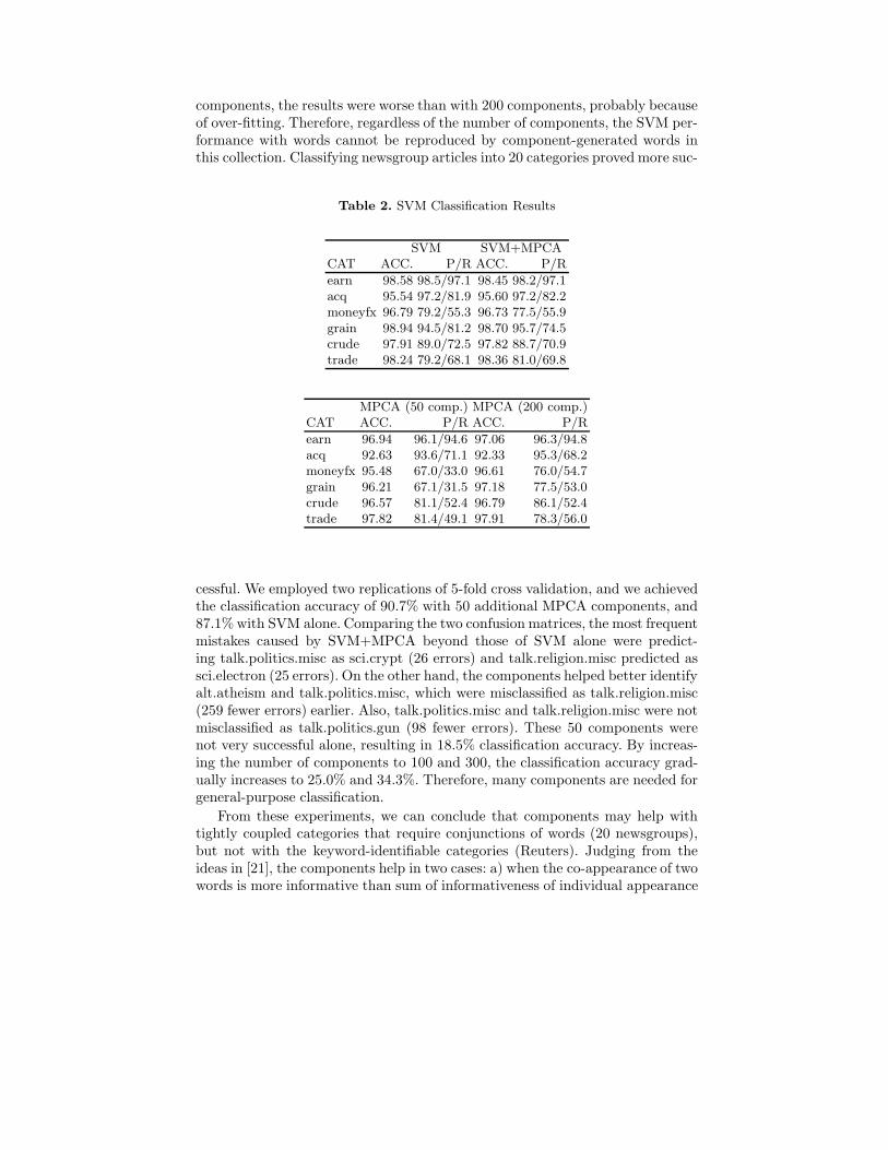
components, the results were worse than with 200 components, probably becauseof over-fitting. Therefore, regardless of the number of components, the SVM per-formance with words cannot be reproduced by component-generated words inthis collection. Classifying newsgroup articles into 20 categories proved more suc-

Table 2. SVM Classification Results

SVM SVM+MPCACAT ACC. P/R ACC. P/R

earn 98.58 98.5/97.1 98.45 98.2/97.1acq 95.54 97.2/81.9 95.60 97.2/82.2moneyfx 96.79 79.2/55.3 96.73 77.5/55.9grain 98.94 94.5/81.2 98.70 95.7/74.5crude 97.91 89.0/72.5 97.82 88.7/70.9trade 98.24 79.2/68.1 98.36 81.0/69.8

MPCA (50 comp.) MPCA (200 comp.)CAT ACC. P/R ACC. P/R

earn 96.94 96.1/94.6 97.06 96.3/94.8acq 92.63 93.6/71.1 92.33 95.3/68.2moneyfx 95.48 67.0/33.0 96.61 76.0/54.7grain 96.21 67.1/31.5 97.18 77.5/53.0crude 96.57 81.1/52.4 96.79 86.1/52.4trade 97.82 81.4/49.1 97.91 78.3/56.0

cessful. We employed two replications of 5-fold cross validation, and we achievedthe classification accuracy of 90.7% with 50 additional MPCA components, and87.1% with SVM alone. Comparing the two confusion matrices, the most frequentmistakes caused by SVM+MPCA beyond those of SVM alone were predict-ing talk.politics.misc as sci.crypt (26 errors) and talk.religion.misc predicted assci.electron (25 errors). On the other hand, the components helped better identifyalt.atheism and talk.politics.misc, which were misclassified as talk.religion.misc(259 fewer errors) earlier. Also, talk.politics.misc and talk.religion.misc were notmisclassified as talk.politics.gun (98 fewer errors). These 50 components werenot very successful alone, resulting in 18.5% classification accuracy. By increas-ing the number of components to 100 and 300, the classification accuracy grad-ually increases to 25.0% and 34.3%. Therefore, many components are needed forgeneral-purpose classification.

From these experiments, we can conclude that components may help withtightly coupled categories that require conjunctions of words (20 newsgroups),but not with the keyword-identifiable categories (Reuters). Judging from theideas in [21], the components help in two cases: a) when the co-appearance of twowords is more informative than sum of informativeness of individual appearance

of either word, and b) when the appearance of one word implies the appearanceof another word, which does not always appear in the document.

8 Conclusion

In this article, we have presented a unifying framework for various approachesto discrete component analysis, presenting them as a model closely related toICA. We have shown the relationships between existing approaches here suchas NMF, PLSI, LDA, MPCA and GaP, and presented the different algorithmsavailable for two general cases, Gamma-Poisson and Dirichlet-multinomial. Forinstance NMF corresponds to a maximum likelihood solution for LDA. Thesemethods share many similarities with both PCA and ICA, and are thus useful ina range of feature engineering tasks in machine learning and pattern recognition.

Acknowledgments

The first author’s work was supported by the Academy of Finland under thePROSE Project, by Finnish Technology Development Center (TEKES) underthe Search-Ina-Box Project, and by the EU 6th Framework Programme in theIST Priority under the ALVIS project. The results and experiments reported areonly made possible by the extensive document processing environment and set oftest collections at the COSCO group, and particularly the information retrievalsoftware Ydin of Sami Perttu. The second author wishes to thank his advisorIvan Bratko. The Mpca software used in the experiments was co-developed bya number of authors, reported at the code website8.

References

[1] L. Azzopardi, M. Girolami, and K. van Risjbergen. Investigating the relationshipbetween language model perplexity and IR precision-recall measures. In SIGIR

’03: Proceedings of the 26th annual international ACM SIGIR conference on Re-

search and development in informaion retrieval, pages 369–370, 2003.[2] R. Baeza-Yates and B. Ribeiro-Neto. Modern Information Retrieval. Addison

Wesley, 1999.[3] J.M. Bernardo and A.F.M. Smith. Bayesian Theory. John Wiley, Chichester,

1994.[4] E. Bingham, A. Kaban, and M. Girolami. Topic identification in dynamical text

by complexity pursuit. Neural Process. Lett., 17(1):69–83, 2003.[5] D.M. Blei, A.Y. Ng, and M.I. Jordan. Latent Dirichlet allocation. Journal of

Machine Learning Research, 3:993–1022, 2003.[6] W. Buntine. Variational extensions to EM and multinomial PCA. In ECML 2002,

2002.[7] W. Buntine and A. Jakulin. Applying discrete PCA in data analysis. In UAI-2004,

Banff, Canada, 2004.

8 http://cosco.hiit.fi/search/MPCA

[8] W.L. Buntine, S. Perttu, and V. Tuulos. Using discrete PCA on web pages. InWorkshop on Statistical Approaches to Web Mining, SAWM’04, 2004. At ECML2004.

[9] J. Canny. GaP: a factor model for discrete data. In SIGIR 2004, pages 122–129,2004.

[10] B.P. Carlin and S. Chib. Bayesian model choice via MCMC. Journal of the Royal

Statistical Society B, 57:473–484, 1995.[11] G. Casella and C.P. Robert. Rao-Blackewellization of sampling schemes.

Biometrika, 83(1):81–94, 1996.[12] J. D. Clinton, S. Jackman, and D. Rivers. The statistical analysis of roll call

voting: A unified approach. American Political Science Review, 98(2):355–370,2004.

[13] M. Collins, S. Dasgupta, and R.E. Schapire. A generalization of principal compo-nent analysis to the exponential family. In NIPS*13, 2001.

[14] J. de Leeuw. Principal component analysis of binary data: Applications to roll-call-analysis. Technical Report 364, UCLA Department of Statistics, 2003.

[15] A. Gelman, J.B. Carlin, H.S. Stern, and D.B. Rubin. Bayesian Data Analysis.Chapman & Hall, 1995.

[16] T.L. Griffiths and M. Steyvers. Finding scientific topics. PNAS Colloquium, 2004.[17] T. Hofmann. Probabilistic latent semantic indexing. In Research and Development

in Information Retrieval, pages 50–57, 1999.[18] T. Hofmann and J.M. Buhmann. Pairwise data clustering by deterministic anneal-

ing. IEEE Transactions on Pattern Analysis and Machine Intelligence, 19(1):1–14,1997.

[19] A. Hyvarinen, J. Karhunen, and E. Oja. Independent Component Analysis. JohnWiley & Sons, 2001.

[20] A. Hyvarinen and E. Oja. Independent component analysis: algorithms and ap-plications. Neural Netw., 13(4-5):411–430, 2000.

[21] A. Jakulin and I. Bratko. Analyzing attribute dependencies. In N. Lavrac,D. Gamberger, H. Blockeel, and L. Todorovski, editors, PKDD 2003, volume 2838of LNAI, pages 229–240. Springer-Verlag, September 2003.

[22] T. Joachims. Making large-scale SVM learning practical. In B. Scholkopf,C. Burges, and A. Smola, editors, Advances in Kernel Methods - Support Vec-

tor Learning. MIT Press, 1999.[23] D. Lee and H. Seung. Learning the parts of objects by non-negative matrix

factorization. Nature, 401:788–791, 1999.[24] D.D. Lee and H.S. Seung. Algorithms for non-negative matrix factorization. In

NIPS*12, pages 556–562, 2000.[25] P. McCullagh and J.A. Nelder. Generalized Linear Models. Chapman and Hall,

London, second edition, 1989.[26] T. Minka and J. Lafferty. Expectation-propagation for the generative aspect

model. In UAI-2002, Edmonton, 2002.[27] F. Pereira, N. Tishby, and L. Lee. Distributional clustering of English words. In

Proceedings of ACL-93, June 1993.[28] K.T. Poole. Non-parametric unfolding of binary choice data. Political Analysis,

8(3):211–232, 2000.[29] J.K. Pritchard, M. Stephens, and P.J. Donnelly. Inference of population structure

using multilocus genotype data. Genetics, 155:945–959, 2000.[30] S.M. Ross. Introduction to Probability Models. Academic Press, fourth edition,

1989.

[31] M.A. Woodbury and K.G. Manton. A new procedure for analysis of medicalclassification. Methods Inf Med, 21:210–220, 1982.

[32] K. Yu, S. Yu, and V. Tresp. Dirichlet enhanced latent semantic analysis. In L.K.Saul, Y. Weiss, and L. Bottou, editors, Proc. of the 10th International Workshop

on Artificial Intelligence and Statistics, 2005.