Discrete Cellular Lattice Assemblycba.mit.edu/docs/theses/15.09.Carney.pdf · Discrete Cellular...

Discrete Cellular Lattice Assembly

by

Matthew Eli Carney

B.S.M.E., CalPoly San Luis Obispo (2004)M.S.M.E., University of California Berkeley (2008)

Submitted to the Program in Media Arts and Sciences, School ofArchitecture and Planning,

in partial fulfillment of the requirements for the degree of

Master of Science

at the

MASSACHUSETTS INSTITUTE OF TECHNOLOGY

September 2015

c÷ Massachusetts Institute of Technology 2015. All rights reserved.

Author . . . . . . . . . . . . . . . . . . . . . . . . . . . . . . . . . . . . . . . . . . . . . . . . . . . . . . . . . . . . . . . . .Program in Media Arts and Sciences

August 7, 2015

Certified by. . . . . . . . . . . . . . . . . . . . . . . . . . . . . . . . . . . . . . . . . . . . . . . . . . . . . . . . . . . . .Neil Gershenfeld

Professor of Media Arts and SciencesThesis Supervisor

Accepted by . . . . . . . . . . . . . . . . . . . . . . . . . . . . . . . . . . . . . . . . . . . . . . . . . . . . . . . . . . . .Prof. Pattie Maes

Academic Head, Program in Media Arts and Sciences


by

Matthew Eli Carney

Submitted to the Program in Media Arts and Sciences, School of Architecture andPlanning,

on August 7, 2015, in partial fulfillment of therequirements for the degree of

Master of Science

Abstract

Robotic assembly of discrete cellular lattices at super-hertz (>1Hz) assembly rates isshown to be possible by integrating the design of a modular robotic assembler with thespecified lattice topology such that the lattice can itself be removed from the incrementalassembly process. Limits to assembly rates are ultimately dependent on allowable error,system stiffness, and damping characteristics. Vibrations due to cyclical motions of theend-effector, locomotion system, and the dynamic response of an incrementally varyinglattice must settle to acceptable ranges to enable engagement between end-effectors,discrete elements, and their affixing features to adjacent cells. For given system dynamics,longer settling times enables greater energy dissipation, and less error. With a greaterallowable error at the interface, a shorter assembly cycle period can be attained. Passivealignment features designed into the robot end-effectors, locomotion systems, and thediscrete lattice elements reduce the precision requirements of the assembly process byopening up the acceptable error range, thereby, enabling higher assembly cycle-rates.An experiment was performed to evaluate how an assembler locally referencing a latticeperformed in comparison to a globally referenced assembler. The two assemblers wereof similar kinematic form: both gantry-type CNC machines: a ShopBot and a custombuilt relative robotic assembler. The results showed superior performance by the globalcoordinate frame system. An error budget analysis of the two systems showed that thelocally referenced, lattice based system had a larger more variable structural loop than theglobal coordinate frame ShopBot. The control experiment, demonstrated 0.1Hz assemblyrates, while first order approximations predict a maximum 4Hz cycle for the specifiedinterface geometry. Results show that in order to successfully assemble discrete cellularlattices at super-hertz rates the robot must itself become the local, instantaneous globalcoordinate frame such that the structural loop is absolutely minimized, while stiffness ismaximized; at the instantaneous moment of assembly the structural loop of the robotmust reference only itself.

Thesis Supervisor: Neil GershenfeldTitle: Professor of Media Arts and Sciences

3


This master thesis has been approved by the following committeemembers.

Neil Gershenfeld . . . . . . . . . . . . . . . . . . . . . . . . . . . . . . . . . . . . . . . . . . . . . . . . . . . . . . . .Chairman, Thesis Committee

Professor of Media Arts and Sciences

Sangbae Kim . . . . . . . . . . . . . . . . . . . . . . . . . . . . . . . . . . . . . . . . . . . . . . . . . . . . . . . . . . .Member, Thesis Committee

Associate Professor of Mechanical Engineering

Brian L. Wardle . . . . . . . . . . . . . . . . . . . . . . . . . . . . . . . . . . . . . . . . . . . . . . . . . . . . . . . .Member, Thesis Committee

Professor of Aeronautics and Astronautics

Acknowledgments

I would like to thank all of my colleagues at The Center for Bits and Atoms. Without

the support of everyone it would not be possible to make cool things happen. I would

also like to thank the folks in the Program in Media Arts and Sciences for their support

to help make cool things happen.

Figure 0-1: The late night crew: Sam Calisch, Will Langford, Ben Jenett, AmandaGhassaei.

7

Contents

1 Introduction 17

2 Robotic Assembler Systems 21

2.1 Automated Assembly . . . . . . . . . . . . . . . . . . . . . . . . . . . . . 21

2.1.1 Common Robot Classifications . . . . . . . . . . . . . . . . . . . 21

2.1.2 Task Specific Assemblers . . . . . . . . . . . . . . . . . . . . . . . 23

2.2 Modular Robotic Systems: Coordinated Assembly of Lattice Structures . 23

2.2.1 Brick Construction . . . . . . . . . . . . . . . . . . . . . . . . . . 25

2.2.2 Active Modules with Passive Truss Elements . . . . . . . . . . . . 26

2.2.3 Relative Robotic Lattice Assembly . . . . . . . . . . . . . . . . . 26

2.3 Global vs. Local . . . . . . . . . . . . . . . . . . . . . . . . . . . . . . . 27

3 Discrete Cellular Lattices 29

3.1 Cellular Lattice Rigidity . . . . . . . . . . . . . . . . . . . . . . . . . . . 30

3.1.1 Kinematic Constraints . . . . . . . . . . . . . . . . . . . . . . . . 32

3.1.2 Modified Maxwell Criteria of Rigid Frameworks . . . . . . . . . . 33

3.1.3 Stiffness of Beams . . . . . . . . . . . . . . . . . . . . . . . . . . . 35

3.1.4 Euler Beam Buckling . . . . . . . . . . . . . . . . . . . . . . . . . 36

3.1.5 Multiphase Cellular Distribution . . . . . . . . . . . . . . . . . . 37

3.2 Stochastic Cellular Lattices . . . . . . . . . . . . . . . . . . . . . . . . . 40

3.3 Non-stochastic Cellular Lattices . . . . . . . . . . . . . . . . . . . . . . . 41

3.3.1 Hierarchical Structures . . . . . . . . . . . . . . . . . . . . . . . . 42

3.3.2 Kagome Structures . . . . . . . . . . . . . . . . . . . . . . . . . . 43

3.4 Discrete Non-Stochastic Cellular Lattices . . . . . . . . . . . . . . . . . . 45

4 Sources of Error 49

4.1 Static Errors . . . . . . . . . . . . . . . . . . . . . . . . . . . . . . . . . . 51

9

4.1.1 Tolerance Analysis . . . . . . . . . . . . . . . . . . . . . . . . . . 51

4.1.2 Total Error Budget Analysis . . . . . . . . . . . . . . . . . . . . . 52

4.1.3 Elastic Averaging . . . . . . . . . . . . . . . . . . . . . . . . . . . 55

4.2 Dynamic Error and Rate Limits . . . . . . . . . . . . . . . . . . . . . . . 57

4.2.1 Servo Loop Time and Stiffness . . . . . . . . . . . . . . . . . . . . 58

4.2.2 Allowable Error and Frequency . . . . . . . . . . . . . . . . . . . 59

4.2.3 Power . . . . . . . . . . . . . . . . . . . . . . . . . . . . . . . . . 63

4.2.4 Control System . . . . . . . . . . . . . . . . . . . . . . . . . . . . 64

5 Comparable High-rate Machines 67

5.1 Qualitative Timing Analysis . . . . . . . . . . . . . . . . . . . . . . . . . 67

5.2 Comparison Machines . . . . . . . . . . . . . . . . . . . . . . . . . . . . 70

6 Implementation 75

6.1 Geometries: Elements and their Interfaces . . . . . . . . . . . . . . . . . 75

6.1.1 Building Blocks . . . . . . . . . . . . . . . . . . . . . . . . . . . . 77

6.1.2 Interfaces . . . . . . . . . . . . . . . . . . . . . . . . . . . . . . . 79

6.2 Geometries: Lattice Topologies . . . . . . . . . . . . . . . . . . . . . . . 82

6.2.1 Face Connected Octahedra . . . . . . . . . . . . . . . . . . . . . . 82

6.2.2 Vertex Connected Octahedra - Cuboct . . . . . . . . . . . . . . . 85

6.2.3 Edge Connected Octahedra . . . . . . . . . . . . . . . . . . . . . 88

6.2.4 Kelvin . . . . . . . . . . . . . . . . . . . . . . . . . . . . . . . . . 88

6.3 Robots: Designs toward dB Scaling . . . . . . . . . . . . . . . . . . . . . 89

6.3.1 Gantry-based . . . . . . . . . . . . . . . . . . . . . . . . . . . . . 90

6.3.2 Mandrel-based . . . . . . . . . . . . . . . . . . . . . . . . . . . . 94

6.3.3 Dynamic Aperture . . . . . . . . . . . . . . . . . . . . . . . . . . 95

6.3.4 Fully Passive . . . . . . . . . . . . . . . . . . . . . . . . . . . . . 98

6.3.5 Hybrid Passive Dynamic . . . . . . . . . . . . . . . . . . . . . . . 99

6.3.6 Tri-helix Locomotion Integrated . . . . . . . . . . . . . . . . . . . 100

7 Conclusions: Future Directions 105

10

List of Figures

0-1 The late night crew: Sam Calisch, Will Langford, Ben Jenett, Amanda

Ghassaei. . . . . . . . . . . . . . . . . . . . . . . . . . . . . . . . . . . . 7

1-1 A robotic assembler of discrete cellular solids, built as a test-case to eval-

uate gantry-based assembly platforms. . . . . . . . . . . . . . . . . . . . 18

2-1 Classification of Automation, clockwise: factory automation [1], humanoids,

robotic fabrication [2], self-assembly [3]. . . . . . . . . . . . . . . . . . . . 22

2-2 Task specific assemblers, counter-clockwise: space truss assembly [4], mod-

ular robotic truss assembly [5], modular robotic [6], automation cell [7],

filament winding [8]. . . . . . . . . . . . . . . . . . . . . . . . . . . . . . 23

2-3 TERMES, modular brick laying robot. . . . . . . . . . . . . . . . . . . . 25

2-4 Shady-3D reconfiguring assembler robot. . . . . . . . . . . . . . . . . . . 26

2-5 AMAS relative assembler robot. . . . . . . . . . . . . . . . . . . . . . . . 27

3-1 Celluar lattices. The left-most image is a stochastic cellular lattice metal

foam [9]. The right-most image is a non-stochastic discrete cellular lattice

designed and built by the author. . . . . . . . . . . . . . . . . . . . . . . 30

3-2 (a) a mechanism; (b) a structure. . . . . . . . . . . . . . . . . . . . . . . 31

3-3 (a) two translations constrained, one rotation free; (b) exactly constrained

two translations and one rotation. . . . . . . . . . . . . . . . . . . . . . . 33

3-4 Perspective sketches of assemblies to illustrate statical and kinematical

determinacy and indeterminacy. . . . . . . . . . . . . . . . . . . . . . . . 34

3-5 (a) Applied bending load; (b) applied axial load; (c) axial load sufficient

to induce buckling. . . . . . . . . . . . . . . . . . . . . . . . . . . . . . . 36

3-6 Cubic octahedron shown as vertex connected octahedra solid phase, tiled

with truncated cubic void phase. . . . . . . . . . . . . . . . . . . . . . . 38

3-7 Cubic octahedron mechanism . . . . . . . . . . . . . . . . . . . . . . . . 40

11

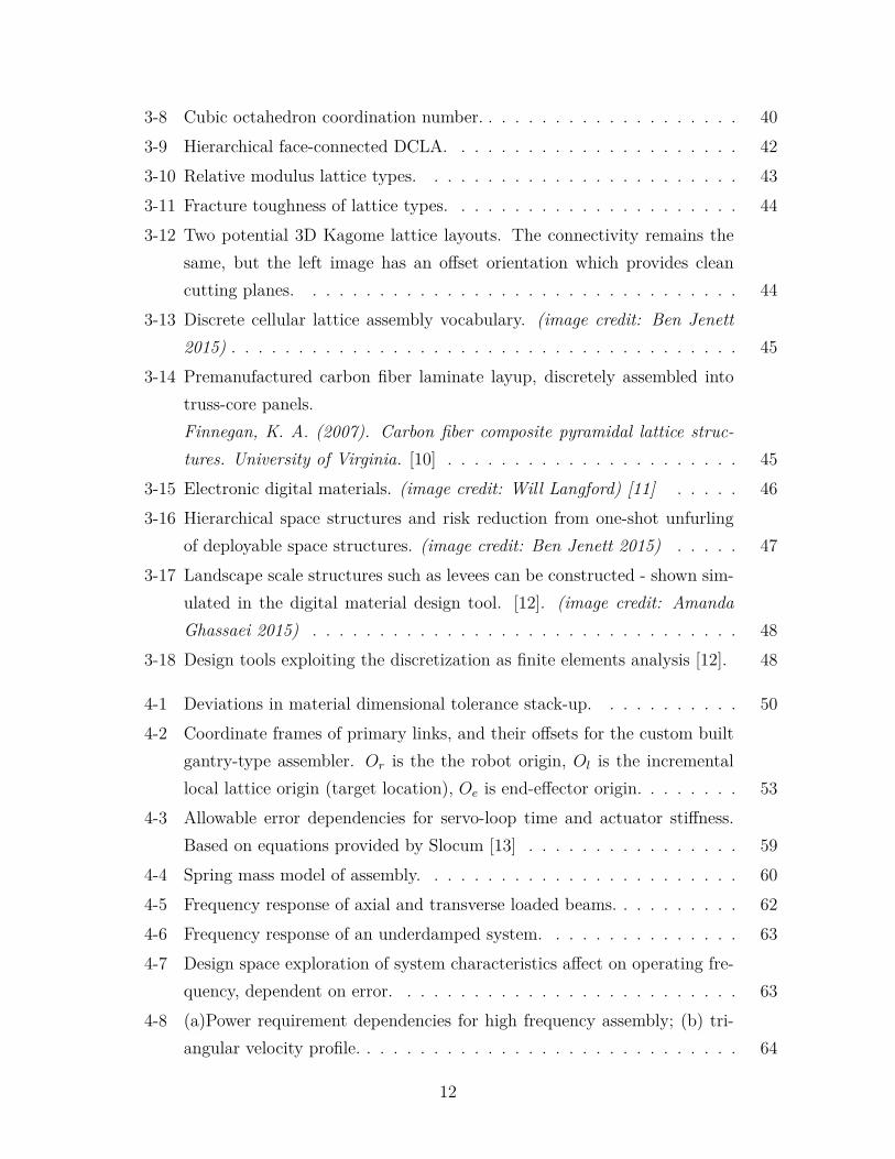
3-8 Cubic octahedron coordination number. . . . . . . . . . . . . . . . . . . . 40

3-9 Hierarchical face-connected DCLA. . . . . . . . . . . . . . . . . . . . . . 42

3-10 Relative modulus lattice types. . . . . . . . . . . . . . . . . . . . . . . . 43

3-11 Fracture toughness of lattice types. . . . . . . . . . . . . . . . . . . . . . 44

3-12 Two potential 3D Kagome lattice layouts. The connectivity remains the

same, but the left image has an offset orientation which provides clean

cutting planes. . . . . . . . . . . . . . . . . . . . . . . . . . . . . . . . . 44

3-13 Discrete cellular lattice assembly vocabulary. (image credit: Ben Jenett

2015) . . . . . . . . . . . . . . . . . . . . . . . . . . . . . . . . . . . . . . 45

3-14 Premanufactured carbon fiber laminate layup, discretely assembled into

truss-core panels.

Finnegan, K. A. (2007). Carbon fiber composite pyramidal lattice struc-

tures. University of Virginia. [10] . . . . . . . . . . . . . . . . . . . . . . 45

3-15 Electronic digital materials. (image credit: Will Langford) [11] . . . . . 46

3-16 Hierarchical space structures and risk reduction from one-shot unfurling

of deployable space structures. (image credit: Ben Jenett 2015) . . . . . 47

3-17 Landscape scale structures such as levees can be constructed - shown sim-

ulated in the digital material design tool. [12]. (image credit: Amanda

Ghassaei 2015) . . . . . . . . . . . . . . . . . . . . . . . . . . . . . . . . 48

3-18 Design tools exploiting the discretization as finite elements analysis [12]. 48

4-1 Deviations in material dimensional tolerance stack-up. . . . . . . . . . . 50

4-2 Coordinate frames of primary links, and their offsets for the custom built

gantry-type assembler. �r is the the robot origin, �l is the incremental

local lattice origin (target location), �e is end-effector origin. . . . . . . . 53

4-3 Allowable error dependencies for servo-loop time and actuator stiffness.

Based on equations provided by Slocum [13] . . . . . . . . . . . . . . . . 59

4-4 Spring mass model of assembly. . . . . . . . . . . . . . . . . . . . . . . . 60

4-5 Frequency response of axial and transverse loaded beams. . . . . . . . . . 62

4-6 Frequency response of an underdamped system. . . . . . . . . . . . . . . 63

4-7 Design space exploration of system characteristics affect on operating fre-

quency, dependent on error. . . . . . . . . . . . . . . . . . . . . . . . . . 63

4-8 (a)Power requirement dependencies for high frequency assembly; (b) tri-

angular velocity profile. . . . . . . . . . . . . . . . . . . . . . . . . . . . . 64

12

5-1 One-Bit Bot, the first interpretation of a relative robotic assembler. . . . 68

5-2 High-speed industrial sewing machine. Note the large crankshaft rotation

driving the needle, cast-iron frame, and the amber cooling oil tube. . . . 71

5-3 High speed bottling machinery. The KHS Innofill filling and capping ma-

chines are the fastest in the industry reaching up to 80,000 bottles per

hour (22Hz). Residence time is increased by passing bottles around a

large circumference. [14, 1] . . . . . . . . . . . . . . . . . . . . . . . . . . 71

5-4 Mass ratio of chassis frame to moving component of comparison machines. 73

6-1 Construction from pure distance and angle constraints. . . . . . . . . . . 78

6-2 Node-to-node connections possible with (a)vertex-connected and (b)face-

connected lattice topologies. In (b) an interface geometry attempts at

passive kinematic alignment: intracellular interface is ball and cone, while

intercellular are tapered faces; both rely on a shear pin for tensile load.

(Dimensions are 100mm node-to-node in both frames.) . . . . . . . . . . 79

6-3 An alignment feature that has Þ polar periodic symmetry, allows more

than a millimeter of deviation in all degrees of freedom and self-energizes

in compression (grid size is 1cm). The broad face, and interlocking nature

of the joint enable moment coupling across the interface. . . . . . . . . . 79

6-4 Joint constraints. . . . . . . . . . . . . . . . . . . . . . . . . . . . . . . . 80

6-5 On the left is a standard issue three-groove kinematic coupling [15]."For

good stability in a three-groove kinematic coupling, the normals to the

planes containing the contact force vectors should bisect the angles be-

tween the balls."[16] . . . . . . . . . . . . . . . . . . . . . . . . . . . . . . 81

6-6 (a) flat elements (PF1) with alignment features; (b) interlocking joint with

additional complexity (OH5). . . . . . . . . . . . . . . . . . . . . . . . . 81

6-7 Kinematic constraints of stacked octahedra. . . . . . . . . . . . . . . . . 84

6-8 Close-up view of node interface for the octa-stack configuration. . . . . . 84

6-9 Face-connected octahedra as a volumetric lattice. . . . . . . . . . . . . . 85

6-10 Mechanical testing of the octa-stack. . . . . . . . . . . . . . . . . . . . . 85

6-11 Cubic-octahedron, or vertex connected octahedra: (a) x-shape element

design with shearpin; (b) square-element with clipped pins; (c) triangle-

element with interlocking fingers. . . . . . . . . . . . . . . . . . . . . . . 87

6-12 Edge connected octahedra with kinematic constraints colored (image credit:

Ben Jenett) . . . . . . . . . . . . . . . . . . . . . . . . . . . . . . . . . . 88

13

6-13 Kelvin Lattice, standard discrete - left, and with reduced degrees of free-

dom, right. (node-to-node spacing is 100mm) . . . . . . . . . . . . . . . 88

6-14 The gantry-based relative robotic assembler (designed and built in March

2015). Also shown with error budget coordinate transformations in figure

4-2. . . . . . . . . . . . . . . . . . . . . . . . . . . . . . . . . . . . . . . . 90

6-15 Maximum frequency of operation with an axially loaded aluminum beam

as an end-effector. . . . . . . . . . . . . . . . . . . . . . . . . . . . . . . . 93

6-16 Global positioning gantry-type assembler. . . . . . . . . . . . . . . . . . . 95

6-17 Mandrel-based assembler . . . . . . . . . . . . . . . . . . . . . . . . . . . 96

6-18 Rack and pinion, dynamic aperature . . . . . . . . . . . . . . . . . . . . 97

6-19 Gear tooth profile . . . . . . . . . . . . . . . . . . . . . . . . . . . . . . . 97

6-20 The geometry of the assembly mandrel passively aligns elements during

placement. Code-name: Zipper . . . . . . . . . . . . . . . . . . . . . . . 98

6-21 A passive mandrel assembler. . . . . . . . . . . . . . . . . . . . . . . . . 99

6-22 A fully integrated locomotion, and placing system where both part place-

ment, and traversal occur simultaneously. Code-name: Leapfrog . . . . . 101

6-23 A prototype of the robot arm mounted single-stage integrated octahedral

turret assembler(a collaboration between Matt Carney and Sebastian Nowak).103

14

List of Tables

5.1 Individual element placement timing estimates for six discrete elements

placed to form a cubic cell. . . . . . . . . . . . . . . . . . . . . . . . . . . 69

5.2 Timing comparison of machines with equivalent motions to assembler robots. 72

6.1 Timing estimates for both placing three elements of a cell, and simultane-

ously traversing to the next cell with a passive loading mandrel. . . . . . 100

6.2 Timing estimates for both placing three elements of a cell, and simultane-

ously traversing to the next cell. . . . . . . . . . . . . . . . . . . . . . . . 102

15

Chapter 1

Introduction

In order for robotic assemblers of discrete cellular lattices (RADCL) to reach super-

hertz (>1Hz) assembly rates the system must operate with a local, instantaneous, global

coordinate frame. Assembly happens without reference to the lattice, at all. The settling

time for allowable error is the greatest limit to assembly rates. To reduce this error

contribution the system must be maximally rigid, with minimal structural loop. There is

no room for the lattice to contribute error, and so it must not. The robot incrementally

ratchets along the lattice, placing cells relative to its own internal coordinate frame.

Robotic assemblers whose kinematic design is directly informed by a lattice topol-

ogy exploit tuning of kinematic and inertial mechanisms for high frequency assembly

and locomotion. Heterogeneous modular robotic systems, or relative robotic assembly of

non-stochastic discrete cellular lattices, provide a primary contrast to traditional man-

ufacturing in that the factory is turned inside out: the object being created is itself

the framework for the factory; the periodic lattice acts as both the desired construction

objective as well as the foundation of locomotion. It is also not self-assembly robotics,

rather wherein self-assembly systems the robot is both the assembler and the structure,

here, the focus is high performance lattice structures assembled by task-specific modular

robots. The complexity of assembly remains within the robot, allowing the lattice to

construct a material that is simple, light weight, and manufacturable at scale.

Large-scale assembly of arbitrarily sized periodic lattice structures lends itself to au-

tomated assembly. This, more so than other manufacturing processes; the environment

of the lattice is highly structured, enabling the automation to be equivalently structured.

Where a traditional industrial robot arm provides a range of functionality, its arrange-

ment of degrees of freedom and inertial characteristics generally serialize the operational

17

capabilities of the system. Kinematic tuning can allow parallelization of assembly se-

quences while minimizing vibrational modes, thereby increasing robustness, and capacity

for higher velocity construction routines. Both the robot, and the structure are defined

with respect to one another, making each one a necessary, and contributing component

to a heterogeneous modular robotic assembly system. Relative robotic assembly enables

unbounded, repairable and reconfigurable construction, along with the computationally

tuned material performance of non-stochastic discrete cellular materials. Discrete cel-

Figure 1-1: A robotic assembler of discrete cellular solids, built as a test-case to evaluategantry-based assembly platforms.

lular lattices are a way of designing, and manufacturing with: ultralight, high stiffness

material regimes [17], reuse and reconfigurability of materials [18], tuned functional per-

formance [11], reduced simulation complexity [19], error correction [20], and automated

assembly. Rather than building large, monolithic, single-use components, the material is

discretized into simple, repeating, functional bits. A discrete set of base elements, with a

discrete set of allowable positions, and orientations are integrated to form non-stochastic

cellular lattices with bulk material properties. In this way, the performance of a material

can be maximized by incrementally assembling high-performance sub-elements. The next

element placed only after the prior, provides in situ error checking and correction. The

order of magnitude difference in wavelength between discrete element, and expressed

cellular solid material properties provides 1√

Nsurface precision. The reconfigurability

maximizes the sustainability post life of the product as it is simply deconstructed, and

reconstructed. Finally, periodicity of structure reduces system uncertainty enabling par-

18

allelization of locomotion, and assembly operations.

The premise for cellular solids operation in the ultralight regime will be explained

along with how the design elements necessary to generate reconfigurable discrete cel-

lular lattices were identified through analysis and experimentation. The discretization

allows reconfigurability of materials yet the interface between individual elements sets

constraints on load paths, as well as the kinematics of assembly automation. The de-

sign of the interface is directly related to the connectivity, and structural performance

of the material. It is also dependent on the total static, and dynamic error budget of

the assembly process; the accumulation of mechanical error from the lattice, through the

assembler machine components, to the interface of the next adjoining element of the lat-

tice, and the dynamic vibration of lattice, and assembler all combine to define minimum

clearance, and ultimately allowable interface designs. These constraints affect the mass,

the stiffness of the system, and ultimately the achievable assembly rates.

By tightly integrating the design of the assembly robot along with that of the dis-

cretized lattice RADCL can be optimized. As is common in robotics, the mutual inter-

dependencies of the subjects must be applied to satisfy the desired goal. The breadth

of this subject requires an introduction to the current state of this emerging field, which

then enables an integration of those concepts into simulated, and built models.

To set the scope, similar heterogeneous reconfiguring modular robotic systems are

introduced. Then, the reader is taken on a dive into cellular materials, with the intention

that they surface with an appreciation for the benefits, and applications for non-stochastic

discrete cellular lattices. The effects of error are so crucial to understanding the demands

of the interface design - which ultimately define dynamic assembly rates - that methods of

tolerance, kinematic constraint, error budget analysis, and vibrations are presented, and

applied, along with a brief section discussing how elastic-averaging enables local error to

become global precision. The learnings from the background chapters are then applied

toward mechanical design experiments performed on lattice topologies, and their associ-

ated inter, and intracellular interfaces. Rather than present all of the work I performed

in this area, I provide a selection of the discovered pivotal design elements, then discuss

them through application, and simulation. 1

To test the above defined dependencies of discrete lattice assembly I built a custom,

relative robotic assembler to test against an off-the-shelf, traditional, linear kinematic,

gantry-type CNC machine. The question asked was: does an assembler that locally

1All work performed was scaled to the same cell dimension, that being the length of an edge of acube encompassing an octahedron: that is 100�� measured across opposing nodes on an octahedron.

19

references a lattice place with more or less precision than a globally referenced assembler?

The experiment consisted of picking up an octahedron voxel from one location, and then

placing it into a target location within an edge-connected octahedral lattice. The two

machines had the same kinematic configuration consisting of linear actuators for x, y,

and z axes. The dependent variable being that the custom built assembler system was

mounted directly on the lattice by way of an incremental relative motion system which

included leg, and foot actuators. The results of the experiment showed, that due to

the increase in uncertainty from the dimensional variability accumulated from the lattice

elements, a local assembler must actually be a locally global assembler.

The conclusion is that the relative robotic assembly process must minimize the struc-

tural loop. The global assembler was more successful in the experiment because the

tolerance stack only ever included its own, tightly controlled, and non-variable, hard-

ware. In order for a robotic assembler that moves relative to the lattice to assemble

locally, the assembler must minimize its structural loop; the assembler must place parts

only relative to itself, without dependency on non-adjacent lattice elements. At each in-

cremental step the assembler must consider that location its instantaneous global origin,

and place adjacent elements with reference to only this instantaneous coordinate frame.

In this way, static dimensional uncertainty is reduced, allowing more room to manage the

positional variability from dynamic conditions, increasing potential assembly rates. The

final chapters utilize this information, and make recommendations of designs for future

relative robotic assemblers to be built and tested.

20

Chapter 2

Robotic Assembler Systems

The use of manipulators for assembly tasks requires that precision with which

parts are positioined with respect to one another be quite high. Current ins-

dustrial robots are often not accurate enough for these tasks, and building

robots that are may not make sense. Manipulators of greater precision can

be achieved only at the expense of size, weight, and cost. The ability to

measure and control contact forces generated at the hand, however, offers

a possible alternative for extending the effective precision of a manipulator.

Since relative measurements are used, absolute errors in the position of the

manipulator and manipulated objects are not as important as they would be

in a purely position controlled system. Since small variations in relative po-

sition generate large contact forces when parts of moderate sitffness interact,

knowledge and control of these forces can lead to a remendous increase in

effecive positional accuracy.

Craig, J. J. (1989). Introduction to robotics : mechanics and control. Read-

ing, Mass. : Addison-Wesley, c1989. [21]

2.1 Automated Assembly

2.1.1 Common Robot Classifications

Robotic automation is used to perform tasks that are either unsafe for humans, or rep-

etitious and require the dexterity of enough degrees of freedoms that it is not feasible

to build a factory-style automation system. Common views of robots are the traditional

six axis industrial robot arm, humanoid or self-assembling modular robots. The exam-

21

ples in figure 2-1 from top right, clockwise show traditional factory automation in a

beer bottling system. The next shows a 6-axis industrial robotic arm, coupled with an

additional 7th rotary axis - this robot is performing advanced computational architec-

tural fabrication, it is machining custom panels for a computationally designed pavilion.

Humanoid robots often have seven degrees of freedom to mimic human range of mo-

tion. Humanoids are designed to operate in unstructured environments, safely, alongside

humans. Self-reconfiguring Modular Robots are combinations of 1-axis modules. The

reconfigurability has been partially driven by a desire to operate in unstructured envi-

ronments where adaptation is necessary. These often move quite slow, and are neither

good at being a robot nor a structure, but are highly adaptable.

All but one of the systems described are generalist, that is their design is such that

they have a multitude of degrees of freedom to enable a variety of applications. This

makes them adaptable for varying tasks, but the serial-link configuration also brings with

it the additional mass of potentially unnecessary degrees of freedom. This additional mass

can limit rates of motion (due to power or vibration limits), as well as limit dexterity in

tight spaces. Task specific assemblers can exploit task specific kinematics.

Figure 2-1: Classification of Automation, clockwise: factory automation [1], humanoids,robotic fabrication [2], self-assembly [3].

22

2.1.2 Task Specific Assemblers

Figure 2-2: Task specific assemblers, counter-clockwise: space truss assembly [4], modularrobotic truss assembly [5], modular robotic [6], automation cell [7], filament winding [8].

Driving for more efficient fabrication modular reconfiguring robotic systems have

been utilized to perform the specific task of assembling arbitrarily sized truss structures.

Trusses are sparse, load bearing systems that are fundamentally, a set of distance and

angle constraints. The system on the right is spiderbot, a space-based, in situ robotic

3D printer of large apperature trusses. Below it is a self contained filament winder for

extruding composite trusses. Beside that is another type of statically mounted truss

extruder that builds with distances and angles. The systems on the left crawl along the

structure and assemble a truss out of discrete elements. In each case the assembly com-

ponents have specific features to aid assembly. These features include passive alignment,

fixturing and even locomotion mechanisms.

2.2 Modular Robotic Systems: Coordinated Assem-

bly of Lattice Structures

One of the grand-challenges of robotics is the design and coordination of multiple robot

systems to cooperatively solve tasks [22] - scalability through parallelization is the fun-

23

damental inspiration. A taxonomy of this new field is still subjective, and best identified

by task goals rather than control architecture. Roughly, system architectures can be

discretized into low-instance coordinated tasks, centralized computation with task dis-

tribution, and decentralized algorithmic coordination – swarms.

Self-assembly, and re-configurable robots have been used interchangeably to describe

both robots that themselves re-configure into new shapes (programmable matter [23]),

and those which are able to compose, and decompose structures. This research focuses

on reconfiguring robots, that is robots acting on lattice structures, but not (generally)

being an integral part of the lattice. In this way the structural performance of the

lattice can be maximized without massive embedded complexity. Similarly, the robotic

assembler can be optimized to assembly tasks specific to the lattice topology, without

the complexity of also being the lattice. The adaptability of structures is highly desirable

for space-based construction where mass can be optimized for final in-space use rather

than launch loading resilience – that is structural elements are packaged for launch and

assembled in-space. Further, localized failures may be compensated or repaired with

reconfigurable systems. Reconfigurability also allows the building of temporary scaffold

structures to allow relatively simple, one-unit-step robots to assemble complex geometries

such as overhangs or pillars [24]. Further, in some instances, the robot may behave as

both the assembler and the structure [25], and be optimized to live, and interact only

within the lattice structure [26]. Optimization between hardware, and path planning is

tightly coupled due to computation, communication, topology, and physical limitations.

Control strategies of swarm systems are generally based on a principle of stigmergy:

In such algorithms, local patterns of matter that result from past construction

provide the exclusive cues necessary to direct and coordinate the building ac-

tivities of the swarm. Therefore, any coherent architecture naturally induces

coordination, which may then be seen as a by-product of the architecture;

more over coordination severely constrains in turn the spaces of possible co-

herent architectures. [27]

Further, a range of control strategies based on stigmergy algorithms may include such

ideas of granular convection, gradients [28], etc. Most of these strategies end up being

relatively similar in the fact that the agents have limited or no knowledge of overall

mission goals but instead stochastically investigate, and assemble based on simple rules.

While, this strategy does allow the construction of structured environments, it is done

without specificity. If detailed custom configuration is necessary then a fully generalized

24

control approach must make use of more centralized control. Strategies range from high

bandwidth communication from fully centralized computation to beacon elements that

manipulate locally generalized construction.

The following is a short survey of the current state of multi-robot coordination for

solving the task of assembly of discrete, cubic, lattice type structures.

2.2.1 Brick Construction

The Self-organizing Systems Research Group at Harvard University has developed a brick

laying robot bioinspired by termite construction techniques, TERMES. "The hardware

comprises a mobile robot and specialized passive blocks; the robot is able to manipulate

blocks to build desired structures, and can maneuver on these structures as well as in

unstructured environments" [24]. The brick morphology of the structure is similar to an

unstructured environment, such as a flat floor or gravel covered field. The bricks contain

kinematic locating features to allow higher placement precision than the robot is, in itself,

capable of providing. Similarly the bricks contain geometry to provide stepping features,

locating, and communication features that provide information to the assembler robot.

Control methodology is based on stigmergy with the modification that agents may be

turned into beacons. This means agents, in general, follow simple rules, however, they

can be locally manipulated to change their path by local beacon information. While the

agents may traverse on unstructured environments, they are gravity based, and as such

are constrained to assemble in ordered fashion. Temporary scaffold structures can be

built to allow complex features such as pillars, and overhangs.

Figure 2-3: TERMES, bio-inspired construction robots.Petersen, K. H., Nagpal, R., & Werfel, J. K. (2011). Termes: An autonomous roboticsystem for three-dimensional collective construction. In Robotics: Science and SystemsConference VII. MIT Press. [24].

25

2.2.2 Active Modules with Passive Truss Elements

A modular robotic system designed to not only build truss structures but to behave as

active elements of the structure; Shady-3D is a three degree of freedom modular robot

that is specified to live within the truss environment it constructs. Reconfigurability of

the structure is a primary element of the design, such that a robotic system "decomposes a

given structure into constituent building blocks and reassembles the same building blocks

into a target structure...[this] approach uses truss structures rather than modular cubic

units, allowing lighter structures and more flexibility in reconfiguration” [29]. Multiple

assembler robots may gang themselves to increase their effective degrees of freedom for

specific tasks. This research is a collaboration between the labs of Hod Lipson at Creative

Machines at Cornell and Daniela Rus at the Distributed Robotics Lab at MIT. Several

iterations of the robots and control algorithms have focused on topological optimization

of the structures. Coordinated assembly, and activation of the structure is optimized

through a quadratic competitive ratio for both static and dynamic graph methods [30].

Figure 2-4: Shady-3D, assembler robot for reconfigurable truss lattice structures.Terada, Y., & Murata, S. (2008). Automatic Modular Assembly System and its Dis-tributed Control. The International Journal of Robotics Research, 27(3-4), 445–462.[30].

2.2.3 Relative Robotic Lattice Assembly

The Automatic Modular Assembly System (AMAS) is a heterogenous modular robotic

construction system. The robotic assemblers are active making motions based on a

finite set of required motions. The building blocks are passive cubic lattice elements,

though they contain mechanisms for mechanical latching, power and communications

transmission. The assemblers locate locally, relative to the structural elements of the

lattice:

The assembler robot can walk on the modules by using connectors on their

26

hands and carrying a module with its hand (L-shaped part). As any modular

structure made up of these modules can be described on a cubic grid, a finite

set of motion patterns is sufficient to build any shape. We took advantage of

this to minimize the configuration of the assembler robot. Only four degrees

of freedom are enough for locomotion and adding a new module on any surface

of another. [31]

Figure 2-5: AMAS assembler robot.Terada, Y., & Murata, S. (2006). Modular stucture assembly using blackboard path plan-ning systems. In International Symposium on Automation and Robotics in Construction(pp. 852–857). [26]

The control strategy is gradient based; a gradient between supply chain and growth

front is communicated to the assemblers to direct their motion. “The desired shape of

the panel is given a priori to both the robot and the structure modules. The modules

can tell whether they are at the growth front, or inside of the shape, and whether their

neighbor point is occupied” [31].

2.3 Global vs. Local

Each of the above modular robotic systems utilize local reference frames for positioning

and locomotion. The premise being the ability to build structures without bound. That

is, by making incremental motions across the structure - assuming an effective method of

material distribution - the scale of structure to be constructed is effectively unbounded.

Repair, and reconfiguration of these structures is also possible with modular robots,

as specific components can be reconfigured in situ, without dissassembly of monolithic

components in a factory. Each of the above robotic systems operate at a scale on the

order of the discrete cell size, or smaller. Each cell provides some alignment features that

27

provide a local position reference. The robot places components only onto the adjacent

cell, and so the precision required is based on the structural loop between only adjacent

cells. This provides a placing accuracy directly related to the precision of two cells.

When it comes to discrete lattice assembly, the assumption is that this local reference

potentially provides higher locational precision than a global scale assembler; the error

stack includes only two adjacent cells, where as global assembly includes the root sum

square of all deviations between the global reference, and the end-effector. That is an

end-effector, whose location is referenced to a single global origin, traversing across a vast

array of cells to a target location may not find the target location in its exact, specified

spot, due to the accumulation of error of each of the discrete cells. There are two possible

options, then to solve this: elastic averaging, and relative placement.

It is possible to have error reduction better than linear when operating locally by

exploiting elastic averaging (see §4.1.3). A modular robotic assembler that spans across

�p parts can express a local precision that is 1√Np

. For a magnitude increase in averaged

accuracy it would require a span across 100 parts - perhaps unrealistic. An error reduction

of one half is potentially possible with four points of contact. It should therefore be

possible to utilize the concepts from modular robotic assemblers of discrete lattices to

design an assembler that has higher positioning accuracy, enabling faster cycle rates (see

§4.2), by utilizing a locomotion system spanning multiples cells.

Alternatively, a further reduction in error can be achieved if the lattice is actually

not part of the structural loop of assembly. If, instead the robot has alignment features

that enable placement only with reference to its own hardware, then the static and

dynamic error contribution from the lattice can be completely removed; the robot latches

onto a lattice cell, and then makes a placement maneuver into the adjacent cell by

mechanically referencing its own hardware. In this way the global origin of the robot

moves incrementally with the robot; at each step its instantaneous local position is its

global reference frame.

28

Chapter 3

Discrete Cellular Lattices

Here we are concerned with lattice or cellular materials. Like the trusses

and frames of the engineer, these are made up of a connected array of struts

or plates, and like the crystal lattice, they are characterized by a typical

cell with certain symmetry elements; some, but not all, have translational

symmetry...At one level, they can be analysed using classical methods of

mechanics, just as any space frame is analysed. But at another we must think

of the lattice not only as a set of connected struts, but as a ‘material’ in its

own right, with its own set of effective properties, allowing direct comparison

with those of fully dense, monolithic materials.

Ashby, M. F. (2006). The properties of foams and lattices. Philosophical

Transactions. Series A, Mathematical, Physical, and Engineering Sciences,

364(1838), p16. [32]

Cellular lattices, low density materials whose properties are defined by the bend-

ing or stretching of load carrying, highly connected, and sparsely distributed structures

with periodic, and translational symmetries [33] [34] exhibit isotropic, anisotropic, or

quasi-isotropic behavior determined by the connectivity of their strut node network [32].

Stretch dominated axial stresses or coupled bending moments are primary material be-

havior indicators that can be identified by the connectivity at nodes and the multiphase

distribution of rigid and mechanism cells throughout the material [35, 36]. "For the lat-

tice to behave as a material, the wavelength of any loading is also much longer than

that of the lattice elements. In contrast, the lattice behaves as a ‘structure’ when it

contains a relatively small number of lattice elements, and the length scale of the loading

is comparable to that of the lattice elements" [37].

29

Primary engineering interest of the cellular lattice is the property of sparse density.

Two distinctly different material behaviors exist within this ultralight regime: energy

absorption, and stiffness [38]. Each property, unique in its cellular structure, application,

and traditionally, in its manufacturing process. Historically engineered uses of cellular

solids have relied on stochastic, bending dominated cellular structures such as honeycomb

and foams, but modern manufacturing techniques enable tuned stretch dominated non-

stochastic lattices that demonstrate an order of magnitude increase in structural efficiency

over bend dominated lattices [35, 39].

This research is primarily concerned with maximizing stiffness and strength of struc-

tures and developing means to assemble lattices from discrete cellular components. The

following is a brief explanation of how the rigidity of a lattice framework is examined and

what underlying scaling variables exist. Then I introduce the variables of importance to

discrete cellular assembly, and how they are effected by the lattice and following chapters

will explain how they effect assembly scalability.

Figure 3-1: Celluar lattices. The left-most image is a stochastic cellular lattice metalfoam [9]. The right-most image is a non-stochastic discrete cellular lattice designed andbuilt by the author.

3.1 Cellular Lattice Rigidity

Analysis of the behavior of cellular lattices requires both a micro and a macro description.

The cellular material has useful engineering mechanical properties that can be treated

as a bulk material with elastic modulus, yield strength, and mass, among other things.

These properties however, are dependent on the aggregate behavior of the cellular lattice

that makes up its microstructure. The most defining attribute of the lattice is how loads

are transmitted through the connecting material that forms the cells, how they connect

to one another, and the distribution of cell types throughout the lattice. The nodes that

are at the interface between load paths can be either exactly, over, or, under constrained.

30

If they are under constrained then an applied load to the lattice, such a compression or

shear will cause the nodes to migrate and the connecting members to bend. If the nodes

are exactly, or over constrained by the load bearing members then those same members

will experience only axial, and no bending loads. This is significant because it results in

an order of magnitude difference in stiffness. Perhaps the best description was given by

Deshpande et al. in the following quote and accompanying figure 3-2:

(a) (b)

joint

strut

F

F F

F

Figure 3-2: (a) a mechanism; (b) a structure. [35]

An open-cell foam can be treated as a connected set of pin-jointed struts

by the following argument. Consider the pin-jointed frames shown in Fig.

1. The frame in Fig. 1(a) is a mechanism. When loaded, the struts rotate

about the joints and the frame collapses; it has neither stiffness nor strength.

The triangulated frame shown in Fig. 1(b) is a structure: when loaded the

struts support axial loads, tensile in some, compressive in others. Thus, the

deformation is stretching-dominated and the frame collapses by stretching of

the struts. Imagine now that the joints of both frames are frozen to prevent

free rotation of the struts. On loading the first frame, the struts can no longer

rotate. The applied load induces bending moments at the frozen joints, and

these cause the struts to bend. This is the situation in most foam structures.

However, freezing the joints of the triangulated structure has virtually no

effect on the macroscopic stiffness or strength; although the struts bend, the

frame is still stretching-dominated and the collapse load is dictated mainly

by the axial strength of the struts.

Deshpande, V. S., Ashby, M. F., & Fleck, N. a. (2001). Foam topology:

bending versus stretching dominated architectures. Acta Materialia, 49(6),

1035.

31

Understanding, now, that the lattice may be treated as a pin-jointed framework of

struts, the traditional next step is to then evaluate the Maxwell rigidity criteria, and

the coordination number for the repeating cell type. Both of these methods evaluate the

kinematic constraint of lattice nodes, yet, the numerical simplifications of geometrical

constraint disregards the mixture of multiphase closed polyhedra (i.e. rigid octahedron

mixed with flexible truncated cubic forms) that necessarily makeup a space filling lattice,

and also help define the operating behavior of cellular materials. The following section

will briefly introduce kinematic constraints which apply both to the understanding of

cellular lattice microstructure, rigid frameworks, as well as later will be directly applied

to discrete cellular lattices.

3.1.1 Kinematic Constraints

An object can move freely in space unless constrained to not move in certain directions by

some fixing force. A 2D object has three kinematic degrees of freedom two translational

and one rotational: �, �, �z. A 3D object has six kinematic degrees of freedom three

translational and three rotational: �, �, �, �x, �y, �z. Structures make use of secondary

rigid bodies to enforce the constraints to limit each of the degrees of freedom. Exact

constraint design, or kinematic constraint design is a design methodology that aims to

constrain each of the required degrees of freedom and only those required, such that

additional internal stresses are not applied to the structure, and that robust, repeatable

precision location of parts is possible [40].

The methodology is straightforward. Each constraint should be effective as a strut

with pins on each end, and acts along a line of action, applying tension or compression

forces and no other. Only translation perpendicular to each line of action is possible. At

the point of intersection of two lines of action there is a rotational degree of freedom,

known as an instantaneous center of rotation. As the point of intersection approaches

the limit of infinity the lines approach parallel and the rotation can be approximated

as a translation. The instantaneous center of rotation is only valid at the instant of

evaluation as it can migrate based on the orientation of the constraint members and their

intersections. In this way, all degrees of freedom can be considered rotations. For each

unwanted degree of freedom a constraint is needed to satisfy the equations of equilibrium.

Further, to form a rigid body framework "each constraint line needs to have a "good size"

moment arm about the instant center of rotation defined by the intersection of the other

two constraint lines" [40].

32

The figure 3-3 shows an under constrained and exactly constrained body. The in-

stantaneous center of rotation is at the intersection of each constraint line, colored light

blue. In frame (a) it is apparent that �, and � are effectively constrained, yet there still

exists a rotational pivot at this arbitrary location on the body shown in blue. The body

is able to rotate about this point, and this point does move based on the orientation of

the body. This system is a four bar linkage. Frame (b) shows a third constraint has

been established that intersects with the x-axis constraint, creating a secondary instant

center of rotation. This new line of action is some "good size" distance from the origi-

nal instant center of (a) and generates a moment that restricts the rotational degree of

freedom that had existed. In this way this framework is now rigid, and each degree of

freedom is exactly accounted for, it is an exact constraint design. If however, an addi-

tional strut were attached to the body in (b) and it had any, even infinitesimal variation

as is always the case in real systems, then all of the members would then be forced into

conditions of self stress as they strain to accommodate the new, over constraint. Any

infinitesimal extension in a strut due to an over constrained structure induces internal

stresses throughout the structure, and is generally considered an undesirable feature in

the mechanical design of structures. The following section shows how Maxwell utilized

these concepts of constraint to apply towards the construction of rigid frames, and how

his framework has since been utilized to predicit the behavior of cellular solids.

Figure 3-3: (a) two translations constrained, one rotation free; (b) exactly constrainedtwo translations and one rotation.

3.1.2 Modified Maxwell Criteria of Rigid Frameworks

Maxwell [41] defined the necessary conditions for a pin-jointed frame of struts to be rigid

statically, and, kinematically determinate in the form a stability criteria. His method-

ology later evolved into exact kinematic constraint as described above [42]. Maxwell

established his rule to define the rigidity of frames, as at the time he was developing

33

precision instrumentation for laboratory equipment, rather than infinite frameworks of

lattices. Nonetheless, it has been shown that a cellular framework can be evaluated as

a system of struts, and pin joints [35]. The rules were updated to include information

regarding not only if the frame was rigid, but if it is bending, or stretch dominated when

the pins are effectively frozen in the nodes of a cellular lattice. The three dimensional

criteria modified to examine the frame stability in terms of mechanisms and self-stress is

given in the following by Pellegrino and Calladine [43]:

� = � ⊗ 3� + 6 = � ⊗ � (3.1)

where, � is number of non-collinear struts, � is number of joints, � is value of self-stress,

� is number of mechanisms. A visualization of what self stress and mechanisms mean

in a framework is seen in figure 3-4.

Figure 3-4: “Perspective sketches of assemblies to illustrate statical and kinematicaldeterminacy and indeterminacy. (a) The three foundation joints lie at the comers of asquare. (b) One bar has now been removed, and the assembly has a mode of inextensionaldisplacement in which the central node moves towards the reader. (c) The fourth barmakes the assembly statically indeterminate. (d.1) A third bar added to (b) makes theassembly both statically and kinematically indeterminate; but only small displacementsof the inextensional mechanism are possible. (d.2) As (d. l), except that the threefoundation joints are colinear, and free motion of the inextensional mechanism, as in (b),is possible.”Pellegrino, S., & Calladine, C. R. (1986). Matrix analysis of statically and kinematicallyindeterminate frameworks. International Journal of Solids and Structures, 22(4), 410.

It should be noted, though, that a similar method of evaluating the behavior of cell

loading conditions that commonly leads to misinterpretation of the Maxwell Criteria is

34

that of coordination or connectivity number, Z, that is the average number of struts

connected to a node. This criteria is used as an explanation for how rigidity can be

defined for an infinite lattice. From coordination number the conditions for rigidity are

Z = 4 for 2D, and Z = 6 for 3D structures[43]. What is commonly forgotten, however, is

that Maxwell’s rule specifically states only non-collinear struts may be evaluated due to

redundancy and the kinematic indeterminance of the equilibrium equations due to strut

collinearity. Figure 3-7 shows a symmetrically sectioned cubic octahedron, showing how

it is in fact a mechanism.

The more accurate Pellegrino and Calladine equation helps us understand the loading

conditions of a cellular lattice. When � < 0, the frame is a mechanism and bending

dominated. When � >= 0, the structure becomes kinematically determinate, and strut

loading conditions are dominantly axial - the frame is stretch-dominated [43].

3.1.3 Stiffness of Beams

The literature has examined through empirical evaluation as well as linear algebraic anal-

ysis that stretch dominated frameworks are an order of magnitude stiffer than bending

dominated, and what conditions must be present in order for a lattice to exhibit such be-

havior. However, one additional factor to explicitly state to help understand the scaling

differences is an examination of the stiffness of a simple beam in each of these loading

conditions: axial, and transverse bending (see figure 4-4).

The distinction between stretch and bending dominated behavior can be further un-

derstood by comparing the stiffness of a solid round beam in axial versus bending load

conditions (figure 3-5). The mechanics for this can be found in most mechanics of mate-

rials or mechanical design references[44, 45]:

�a =��

�(3.2)

�b =3��

�3(3.3)

Where, for a round slender member, � << �, and inserting

� =Þ�2

4

� =Þ�3

64

35

back into the stiffness equations

�a =��

�=

Þ�

4

⎠

�2

�

⎜

(3.4)

�b =3��

�3=

3Þ�

64

⎠

�2

�

⎜21

�(3.5)

it can be seen that axial stiffness is related to a beam slenderness ratio d2

Lby an order

of magnitude scaling �(d2

L) = �(1). The bending stiffness of the same beam is then a

two order of magnitude �(2) scaling of this slenderness ratio, and additionally, inversely

proportional to the length of the beam.

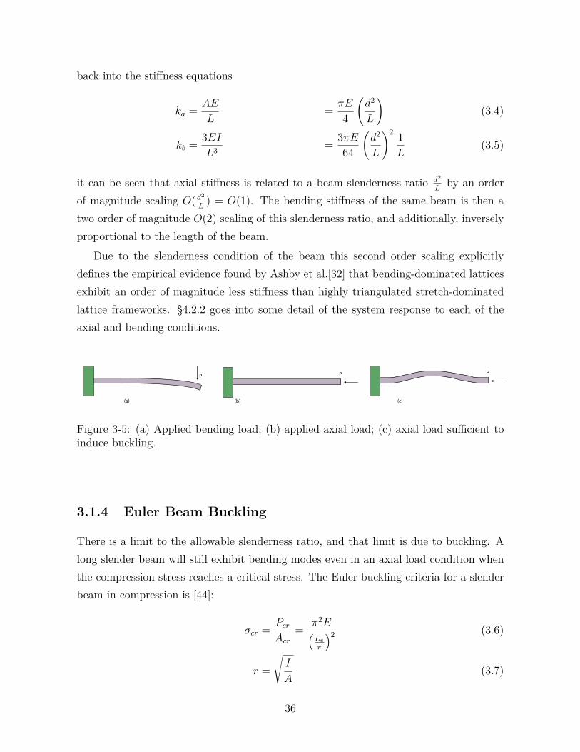
Due to the slenderness condition of the beam this second order scaling explicitly

defines the empirical evidence found by Ashby et al.[32] that bending-dominated lattices

exhibit an order of magnitude less stiffness than highly triangulated stretch-dominated

lattice frameworks. §4.2.2 goes into some detail of the system response to each of the

axial and bending conditions.

P

(a) (b) (c)

PP

Figure 3-5: (a) Applied bending load; (b) applied axial load; (c) axial load sufficient toinduce buckling.

3.1.4 Euler Beam Buckling

There is a limit to the allowable slenderness ratio, and that limit is due to buckling. A

long slender beam will still exhibit bending modes even in an axial load condition when

the compression stress reaches a critical stress. The Euler buckling criteria for a slender

beam in compression is [44]:

àcr =�cr

�cr

=Þ2�⎞

Le

r

︁2(3.6)

� =

︃

�

�(3.7)

36

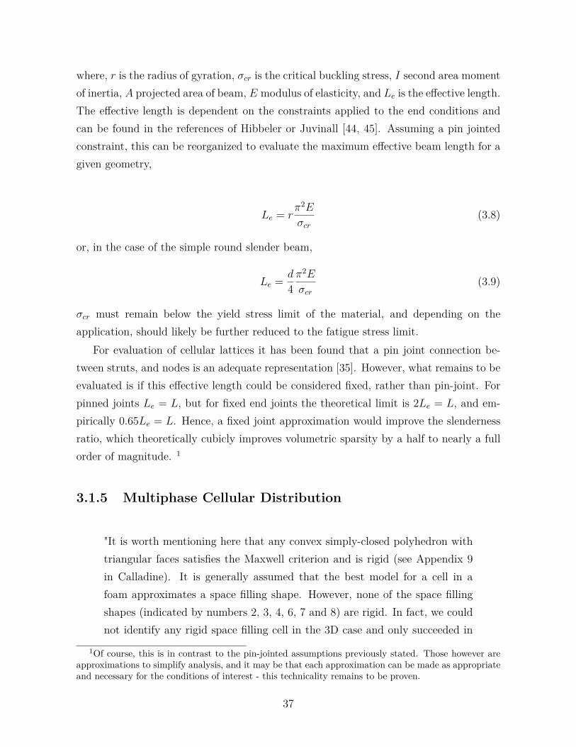
where, � is the radius of gyration, àcr is the critical buckling stress, � second area moment

of inertia, � projected area of beam, � modulus of elasticity, and �e is the effective length.

The effective length is dependent on the constraints applied to the end conditions and

can be found in the references of Hibbeler or Juvinall [44, 45]. Assuming a pin jointed

constraint, this can be reorganized to evaluate the maximum effective beam length for a

given geometry,

�e = �Þ2�

àcr

(3.8)

or, in the case of the simple round slender beam,

�e =�

4

Þ2�

àcr

(3.9)

àcr must remain below the yield stress limit of the material, and depending on the

application, should likely be further reduced to the fatigue stress limit.

For evaluation of cellular lattices it has been found that a pin joint connection be-

tween struts, and nodes is an adequate representation [35]. However, what remains to be

evaluated is if this effective length could be considered fixed, rather than pin-joint. For

pinned joints �e = �, but for fixed end joints the theoretical limit is 2�e = �, and em-

pirically 0.65�e = �. Hence, a fixed joint approximation would improve the slenderness

ratio, which theoretically cubicly improves volumetric sparsity by a half to nearly a full

order of magnitude. 1

3.1.5 Multiphase Cellular Distribution

"It is worth mentioning here that any convex simply-closed polyhedron with

triangular faces satisfies the Maxwell criterion and is rigid (see Appendix 9

in Calladine). It is generally assumed that the best model for a cell in a

foam approximates a space filling shape. However, none of the space filling

shapes (indicated by numbers 2, 3, 4, 6, 7 and 8) are rigid. In fact, we could

not identify any rigid space filling cell in the 3D case and only succeeded in

1Of course, this is in contrast to the pin-jointed assumptions previously stated. Those however areapproximations to simplify analysis, and it may be that each approximation can be made as appropriateand necessary for the conditions of interest - this technicality remains to be proven.

37

synthesising rigid periodic 3D frameworks from combinations of rigid cells

(e.g. the tetrahedron and octahedron in combination fill space to form" [32]

Figure 3-6: Cubic octahedron shown as vertex connected octahedra solid phase, tiledwith truncated cubic void phase.

What Ashby is referring to is that while triangulated polyhedra do satisfy the Maxwell

criterion, there are only two shapes that self fill space, rigidly. In fact the only known

regular polyhedra to fill space are the cube, tetrahedra, and octahedra [46]. This means,

since foams do fill space with closed polyhedra forms, there results a mixture or multi-

phase configuration of different polyhedra shapes that fill the volume. The multi-phase

arrangement may then be composed of statically rigid, fully constrained polyhedra, and

polyhedra of varying mechanism.

The effective elastic moduli of such multi-phase materials are approximated by the

strain energy bounds of the Hashin-Shtrikman variational principles of mixtures. Shown

below is the simplification for a two phase mixture [36].

�e

�=

�ã

�(1 ⊗ ã) + �(3.10)

�e

�=

�ã

(� + 2�)(1 ⊗ ã) + �(3.11)

where, ã is a solid volume fraction, 1 ⊗ ã void phase volume fraction, � bulk modulus,

�e effective bulk modulus, � shear modulus, �e effective shear modulus [36, 47].

As the void phase volume fraction approaches zero the cellular material behaves as

its stretch-dominated rigid polyhedra dictates. However, for mixed phase cellular lattices

there exists a derating of rigidity due to the mixture of rigid and mechanism frameworks.

38

This derating effect can make a solid phase rigid cellular lattice and make it minimal

rigid [35].

Some examples of this shown in figure 3-6 are the cubic octahedron tiling system

that includes node connected octahedra (rigid), mixed with truncated cubes (mecha-

nism void). The octahedron is a fully triangulated six joint, twelve strut, structure; it

is exactly constrained with zero self-stress, zero mechanisms, and demonstrates stretch-

dominated behaviour. The octahedron can be assembled in different density configura-

tions: vertex-connected, edge-connected and face connected. Each configuration nesting

with a different type of volume filling space: a truncated cube, tetrahedron and tetra-

hedral dipyramid. However, as a mixture of rigid, closed polyhedra is not necessarily

rigid.

In this example the octahedra are rigid, and in planar tension/compression the lat-

tice remains so. However, the truncated cubic void phase volume fraction expresses three

degree of freedom mechanisms (rotations about each axis). In planar shear, the vertex

connected octahedra solid phase has a single constraint that lies along the plane perpen-

dicular to the shear, while the void phase has a mechanism, such that the shear response

of the cubic octahedra (the cuboct) comes from a pure bending load condition on the

strut members of they are frozen in their joints. Another way to look at this mechanism

to reference figure 3-7 where Pellegrino and Calladine demonstrate how a cross sectioned

cubic octahedron can seemingly satisfy the Maxwell criteria yet be statically and kine-

matically indeterminate. Finally, it is also apparent from figure 3-8 where it is clear that

the node connectivity only constrains translational modes, while rotational modes are

free. From this analysis we see a vertex connected, cubic octahedron has been shown to

be a minimum density, maximum axially stiff lattice yet identified [17], but may only

be axially stiff; it is quasitropic, axial loading is stretch dominated, shear is bending

dominated.

That said, according to Deshpande et al. a rigid boundary condition can be considered

part of the volume fraction, and will play a part in overall system stiffness. For instance,

a rigid boundary can assert distance constraints on the boundary nodes, restricting the

expression of a structural mechanism that would otherwise exist. This example surface

rigidity constraint, however, becomes inconsequential as the volume increases such that

the fraction of the rigid boundary condition phase becomes insignificant, and the void

phase volume fraction approaches a significant contribution to the total solid volume. The

system then approaches a minimal stiffness condition for the specified loading conditions

39

[35].

Figure 3-7: "(a)A ring assembly [or cross sectioned cubic octahedron] which satisfiesMaxwell’s rule, but (b) is statically and kinematically indeterminate with a free mecha-nism of inextensional displacement."Pellegrino, S., & Calladine, C. R. (1986). Matrix analysis of statically and kinematicallyindeterminate frameworks. International Journal of Solids and Structures, 22(4), 410.

Figure 3-8: Although an octahedron is statically and kinematically constrained, whenstacked vertex to vertex there remain three degrees of freedom about the vertex. Acommon accounting error is to double count the collinear struts coming from the node.Here it would appear that this configuration has a coordination number of Z=8, but infact it is Z=4. The node or vertex is constrained in 2D, but there remain three rotationaldegrees of freedom about it.

3.2 Stochastic Cellular Lattices

Stochastic cellular lattices may exist in open or closed cell forms. These cellular lattices

occur in nature in the form of honeycomb, bones, woods, etc., and have been synthesized

in the lab, and factory from polymers, ceramics, and metals [38]. Their performance is

generally characterized by energy absorption, space filling capabilities, anf high surface to

volume ratios. The low density space filling property has been of particular interest to the

aerospace industry for its ability to stiffen composite panels by providing buckling support

40

to thin wall composite designs, allowing higher second area moment of inertia structural

geometries [48]. The macroscopic strength of such materials is based on the microscopic

lattice connectivity, which in the case of cellular foams is bending dominated. Due to the

reduced stiffness of bend loading (see 3.1.3) compared to axial tension, the linear elastic

stiffness characteristics of open and closed cell foams scale with relative density �̄2 and �̄3,

respectively [33]. When applied towards stiffening applications stochastic cellular solids

provide non-optimal elastic modulus, and density scaling properties [48]. The limitation

to stochastically assembled lattices in ultralight stiff material regimes is the existence of

non-homogenous cellular distributions of voids; cellular topology variation compromises

structural efficiency by creating undesired multiphase lattice structures. Finally, because

"a low-connectivity lattice, typified by a foam, with a relative density of 0.1 (meaning that

the solid cell walls occupy 10% of the volume) is less stiff by a factor of 10 than a stretch-

dominated, triangulated lattice of the same relative density," [32] the engineer in search

of an optimal, ultralight, stiff, and strong structural framework looks to non-stochastic,

or ordered, cellular lattices.

3.3 Non-stochastic Cellular Lattices

Non-stochastic stretch-dominated cellular lattices can be designed to operate with a linear

relationship between stiffness and relative density, allowing the already stated (section

3.1.3) magnitude increase in stiffness to mass over traditional foam materials [32, 35,

37]. By combining rigid, and semi-rigid (rigid as defined by Maxwell, a statically and

kinematically determinate framework, where semi-rigid is kinematically indeterminate

and therefore can express a mechanism) space filling forms the overall characteristics

of the materials can be tuned to specific performance. Combinations of space filling

tetrahedra, octahedra, and other non-rigid, under-constrained frameworks enable tuning

of stiffness and degrees of freedom, allowing controlled anisotropic behaviors enabling

energy absorption or morphing structures. It has been conjectured that, because these

non-stochastic structurse can be made to be kinematically determinate, manipulation

of these structures by replacing some strut members with actuators may even result

in materials that perform controlled mechanical behaviors [49]. A great deal of work

has been published regarding the use of 2.5D lattices as the core of structural panels of

composites or metals [50, 51]. Continuous processes have also been utilized with fiber

wrapped structures [52]. Additive manufacturing processes have allowed the construction

41

of 3D lattices in combinations of polymer or polymer core, metal coated structures. Of

great interest further is the construction of multi-scale hierarchical structures that follow

the same construction rules at multiple scales [53] to further maximize material sparsity,

and at the nano level, exploit material nonlinearities. Hierarchy has been applied at nano

[54], micro [55] and macro [53] scales.

3.3.1 Hierarchical Structures

Figure 3-9: Hierarchical structure built from the OT6 discrete cellular lattice elements.Length scales from 5cm to 1m by building columns of face-connected octahedra termi-nated with tetrahedra. This is the same geometry as Rayneau-Kirkhope et al. [55] exceptfabricated with reconfigurable discrete cellular lattices. Far right is a notional image ofspace-scale structures (parts/image credit: Matt Carney/Benjamin Jenett 2015).

Second order hierarchical structures have been shown to exhibit an additional order of

magnitude increase in stiffness to mass over first order cellular lattice assemblies when op-

erated in low-load conditions - a property directly applicable to space structures that are

often stiffness limited [53]. Both Murphy and Rayneau-Kirkhope et al. show optimization

of self-similar hierarchy settling on second order configurations at both macro and micro

scales. Rayneau-Kirkhope et al. found an optimal strut member to be a column of face

connected octahedra terminating at the 2nd order nodes with tetrahedra. One potential

drawback they found, however [56], was any failures occurring at the first order lattice

affected system stability at the following hierarchical orders. This likely due to the exact

constraint of the geometry having limited redundancy. Hierarchical structures have also

been created with a continuous fiber wrap process and has similarly demonstrated local

and global buckling behavior[52]. That said, hierarchical structures can further exploit

deterministic lattice behavior such as tuned stiffness, strength and failure resilience by

combining combinations of stretch and bend dominated lattice geometries [37, 55, 56].

42

3.3.2 Kagome Structures

Figure 3-10: "Relative modulus plotted against relative density on logarithmic scales forcellular structures with alternative topologies. Bending-dominated structures lie along atrajectory of slope 2; stretch-dominated structures along a line of slope 1."Ashby, M. F. (2006). The properties of foams and lattices. Philosophical Transactions.Series A, Mathematical, Physical, and Engineering Sciences, 364(1838), 27.

When filling space with sparse structures, and with a goal to maximize isotropic stiff-

ness while filling the space one would like to find the optimal configuration of closed

polyhedra. Similarly, in order to have isotropic properties one supposes it is best to

find regular polyhedra that fill the space. Asking this question it was found that for

a 2D topology optimization "Kagomé-like cellular solids will have superior strength to

the elastic buckling loads than either triangular-like or hexagonal-like cellular solids" and

has "optimal elastic moduli in the zero-density limit" [47], in planar loading. Further,

Ashby found the Kagome structure represents the upper limit to achievable strength to

relative density, figure 3-10, [32] while Fleck et al. found it is the maximum stiffness

to relative density, and also fracture toughness for cellular lattice materials, figure 3-11

[37]. However, these analysis were performed on planar loading, without disturbance.

The connectivity of nodes is Z=3 in 3D, which leaves three rotational degrees of freedom.

Due to these degree of freedom the structure is actually a combination of bending and

stretching. Which, is how it receives high scores for overall toughness, by combining

elongation and bending loading conditions [57, 49]. The literature shows a variety of

different structures that claim to be 3D Kagome, which include variations of tessellated

43

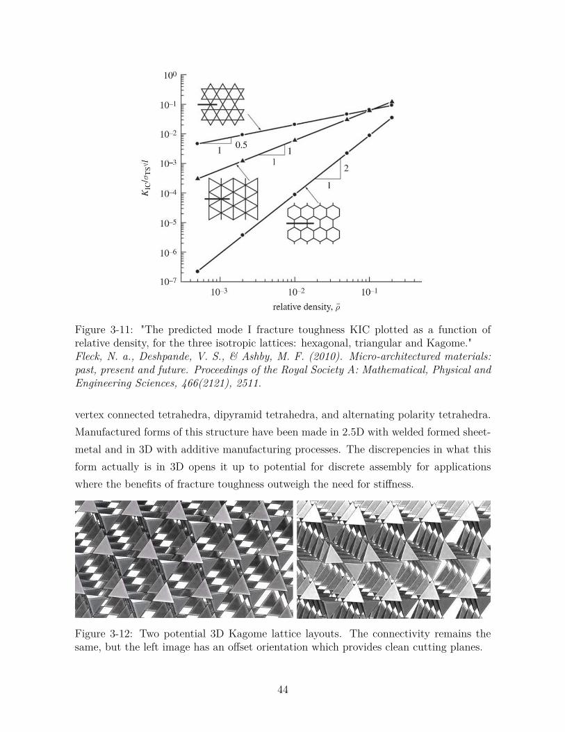
Figure 3-11: "The predicted mode I fracture toughness KIC plotted as a function ofrelative density, for the three isotropic lattices: hexagonal, triangular and Kagome."Fleck, N. a., Deshpande, V. S., & Ashby, M. F. (2010). Micro-architectured materials:past, present and future. Proceedings of the Royal Society A: Mathematical, Physical andEngineering Sciences, 466(2121), 2511.

vertex connected tetrahedra, dipyramid tetrahedra, and alternating polarity tetrahedra.

Manufactured forms of this structure have been made in 2.5D with welded formed sheet-

metal and in 3D with additive manufacturing processes. The discrepencies in what this

form actually is in 3D opens it up to potential for discrete assembly for applications

where the benefits of fracture toughness outweigh the need for stiffness.

Figure 3-12: Two potential 3D Kagome lattice layouts. The connectivity remains thesame, but the left image has an offset orientation which provides clean cutting planes.

44

3.4 Discrete Non-Stochastic Cellular Lattices

Figure 3-13: Discrete cellular lattice assembly vocabulary. (image credit: Ben Jenett2015)

Although it has been shown that for designs operating in the ultra-light regime non-

stochastic cellular lattices are a primary material choice, their scalability in application,

and sub-material options can be reliant on limited additive manufacturing processes. To

build at substantial scale, components must be batch processed, and fit together with

some discontinuous interface. This type of bulk production generates monolithic, high

value components - transportation, and handling of these can be costly, and risky. One

way to potentially address these issues is to plan on the discontinuous interface, integrate

it fully into the structure, and discretize the lattice geometry entirely into its fundamental

building blocks.

Figure 3-14: Premanufactured carbon fiber laminate layup, discretely assembled intotruss-core panels.Finnegan, K. A. (2007). Carbon fiber composite pyramidal lattice structures. Universityof Virginia. [10]

Discrete cellular lattices (digital materials) are a way of designing and manufacturing.

Rather than building large, monolithic, single-use components, the material is discretized

into simple, repeating, functional bits. The individual elements pack densely and are then

unpacked into sparse, performance structures. The discrete set of base elements, with a

discrete set of relative positions, and orientations are combined to form cellular lattices

that perform as bulk materials. Building the lattice one structural element at a time

45

with robust load bearing interfaces enables utilization of all known material, and man-

ufacturing processes, allowing for highly tuned structures [10]. While local variations

exist, bulk precision elastically averages out (§4.1.3), providing overall precision greater

than the placement of the individual blocks. This discretization provides assurance of

the structural capacity of the final bulk material by allowing the use of tightly con-

trolled manufacturing environments for the construction of each discrete element; tightly

controlled manufacturing process gives assurance of individual element performance, al-

lowing prediction and control of their failure, and therefore the ultimate failure of the

bulk structure. It also allows the combination of heterogeneous material combinations,

as well as the opportunity for reconfiguration of materials and structures for repair or

re-purpose. Local metrology is physically encoded in the geometry of mating surfaces;

the placement of each component can be controlled, checked, and recorded - error cor-

rection is in situ to manufacture. These processes are not entirely-unlike, and inspired

by ribosomal amino acid construction.

The discretization of the lattice enables combinations of heterogeneous elements that

include varying stiffness as well as embedded functionality. When enclosed-area elements

are utilized there is space reserved for housing additional features such as sensing, and

actuation. Further, electrical connectivity could be molded into the individual elements

enabling distributed power generation and health monitoring of structures. Langford

has shown that elements can themselves be made electrically functional: conductive,

semi-conductive, and non-conductive combined into discrete electronic components [11].

Figure 3-15: Electronic digital materials. (image credit: Will Langford) [11]

Automated assembly is paramount to the scalability of manufacture of high part-count

structures. A major win comes from the simplicity provided by a structured environment

for the assembly robots. The lattice, being a lattice, provides local metrology, enabling

both global and local coordinate frame assembly machines. Just as a factory is tuned to a

46

specific product line, relative robotic assemblers of discrete lattices are tuned to the lattice

geometry. Operations, and kinematics are performed in parallel, rather than serially,

increasing system stiffness and throughput. That is to say, rather than constructing a

product inside a factory, the factory will consist of swarms of highly tuned robots crawling

incrementally across the lattice, assembling and disassembly as necessary. While some

systems may still benefit most from the rigidity and control of a factory, the most severe

benefit comes to the construction of objects that do not fit within the confines of a factory.

Space-structures are limited by deployment mechanisms. The unfurling behavior requires

Figure 3-16: Hierarchical space structures and risk reduction from one-shot unfurling ofdeployable space structures. (image credit: Ben Jenett 2015)

substantial mechanical features consuming limited launch mass and volume availability,

limiting the range of their deployable reach. Additionally, space structures are designed

to withstand launch forces, conditions only ever experienced once in their operational

lifetime. These load requirements unnecessarily increase the mass of the systems - cost.

Discrete lattice elements are designed to be flat-packed for efficient transportation, and

autonomously unpacked once in space. The incremental, and error correcting nature

of the construction system enables unbounded-scale space construction with continuous,

but incremental unpacking of resupply shipments of lattice elements. Landscape scale

structures would be the next architecture to be unbounded from the factory: bridges and

levees. Both infrastructural improvements that benefit from sparse density, high stiffness,

simplified transportation and assembly. Both infrastructures also are in dire need of repair

in the United States and would benefit highly from an automated assembly system that

can operate without stop - integrating its work effort over a longer period than humans

are capable. Bridges possibly more likely to come sooner than levees however because

they benefit from a structured foundation; the pivotal technology of the robotic assembler

of discrete lattices is the highly structured environment. Assembly nucleates from a seed;

a foundation of some sort is necessary. Bridge construction would be a strong impedance

match for this technology as it provides a formulated anchor and benefits greatly from

47

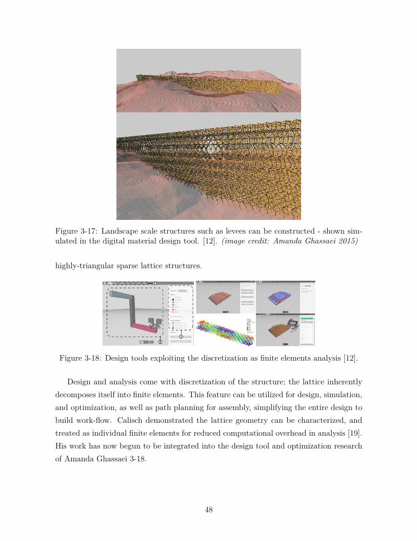
Figure 3-17: Landscape scale structures such as levees can be constructed - shown sim-ulated in the digital material design tool. [12]. (image credit: Amanda Ghassaei 2015)

highly-triangular sparse lattice structures.

Figure 3-18: Design tools exploiting the discretization as finite elements analysis [12].

Design and analysis come with discretization of the structure; the lattice inherently

decomposes itself into finite elements. This feature can be utilized for design, simulation,

and optimization, as well as path planning for assembly, simplifying the entire design to

build work-flow. Calisch demonstrated the lattice geometry can be characterized, and

treated as individual finite elements for reduced computational overhead in analysis [19].

His work has now begun to be integrated into the design tool and optimization research

of Amanda Ghassaei 3-18.

48

Chapter 4

Sources of Error

All mechanical systems have dimensional variation due to their manufacturing processes.

One part off of a press, or a CNC machine, or any other manufacturing equipment will be

slightly different from the next part, and the previous part. These are small local errors,

Ó, and a production lot of parts have statistical means, Û, and standard deviations,

à. A mechanical system, composed of a multitude of mechanical parts will have some

variation in its overall dimensional accuracy when compared to another system of the

exact same design made from parts that came off of the exact same manufacturing line.

The dimensional variation of each part in the assembly of the mechanical system adds to

the overall system variation. The act of assembling two parts also introduces uncertainty

based on: how flat the surfaces are, if dust or something larger slipped between the

mating surfaces, how tight the bolts are - if they are warping the geometry of the parts

they fasten - what the temperature in the room was when they were assembled, and

more. These are variations internal to a single mechanical assembly, which itself may be

a subassembly that gets assembled amongst other systems to combine into some more

complex machinery such as a toaster, an airplane, or a robot.

In order for sub-assemblies to properly fit within the context of their larger roles as

machine subsystems, the other parts of the machine must be designed to tolerate the

statistical variation of dimensions, and performance, of the to be inserted components

such that there is adequate room for the subassembly to fit. Yet, the fit must still

be substantially precise enough that there remains adequate accuracy in alignment for

further assemblies, and adequate holding force by the fastening system. This cascade

of sub-assemblies becomes a structural loop. There is some critical point that can be

considered the origin of this structural loop, and it is here at this point that the stack-

49

δ1

δ2

δ3

δ4

δ0

δ1

δ2

δ3

δ4

δ0

δ1

δ2

δ4

δ0

Figure 4-1: Deviations in material dimensional tolerance stack-up. The left shows howà0 must be designed and manufactured such that the combination of à1, à2, à3 still allowthe new part with dimension à4 to fit securely, but not too loose. The right image showshow the structural loop and dynamics of the assembler further contribute to the tolerancerequirements of the interface.

up of errors from this structural loop is evaluated. From this structural loop analysis

a design must be implemented that tolerates these system variations. Parts can have

varying degrees of effect on the total system error, if for example there are angular

alignment errors, abbe errors, [13] in a serially stacked system, then those small angular

defects can be amplified by their serially stacked lever arm, having significant impact

at the positional accuracy at the end of the chain. An error budget analysis can be

performed to analyze the impact of errors to identify the overall performance, or what

are adequate design consideration to be made such that desired overall performance can

be attained.

Static errors, due to manufacturing and assembly combine with dynamic errors from

operational conditions to generate uncertainty at the end effector or point of interest.

Static or quasi-static errors come from the manufacturing, and assembly variations. These

errors exist due to random variation, systematic, and hysteretic variation. They effect

the overall system accuracy, can often be managed through design, measurement, and

closed-loop feedback. Dynamic errors dictate how fast a machine may operate. The stiff-

ness of the structure, actuators, their natural frequencies, mass of moving objects, and

motor dynamics define an operational stability. In the case of a robotic assembler, the

rate at which it may operate is a balance between the time constant to stabilize within

a specified dimensional tolerance, and what is an allowable dimension the part interface

can tolerate while maintaining its desired structural performance. The more mass or the

faster the mass needs to move the larger the acceleration that must be generated by the

50

actuator. The reaction force from the actuator to the structure induces vibrations. The

amplitude of force combined with the rate of actuation must be out of range of system

natural frequencies, else large amplitude vibrations may be induced. These vibrations

lengthen settling time, and contribute to end-effector positional accuracy oscillations.

Alternatively, it is possible to design systems that attempt to reduce the effects of dy-

namic errors by operating in regimes outside of system natural frequencies, by building

stiff, damped, vibration tolerant designs.

4.1 Static Errors

4.1.1 Tolerance Analysis

All parts exhibit some fluctuation in size due to the normal distribution of variation from

manufacturing processes. When multiple parts are stacked into assemblies and are then

to fit together within another assembly their total variations must be accounted for in the

design of receiving assembly, else the fit will not be robust or even possible. This stack

of parts make up a structural loop, and their variations can be considered a tolerance

stack, visualized in figure 4-1. The total contribution to error of the series of variations

can be estimated by making use of a Root Sum Square (RSS) of the standard deviation

of the errors of each of the individual parts in the stack. In modern manufacturing

terms the preference is for six sigma design principles, where parts are designed to fit

together accommodating six standard deviations of variation, guaranteeing 99.9999998%

reliability fitting interfaces. Motorola found that this six sigma process really depends on

short term variation. That is, over long term distribution the mean might migrate ∘1.5à,

but manufacturing process should identify and fix these process defects, and as such

short term 6àST is a valid. Common practice is to design with traditional manufacturing

tolerances in mind, traditionally documented from a three sigma longterm distribution.

Design principles from a modern consumer electronics manufacturer suggest a conversion

between long term and short term distributions with a simple ∘1.5. This distribution

is generally acceptable to be used in analysis of clearance requirements, but must be

51

evaluated based on the needs of the product. [58]

à =

⎠

N︁

i=1

à2

i

⎜

1

2

(4.1)

àST = 1.5

⎠

N︁

i=1

à2

i,LT

⎜

1

2

(4.2)

In the case of discrete cellular lattice assembly there are very large numbers of individ-

ual parts that must be assembled to fit together. Statistical variations become significant

with large volumes of assembled parts. The reliability of the interfaces, as well as the

stacks of components must be designed such that robust fixturing is possible with the

dimensional distributions expected from manufacturing processes.

The number of standard deviations necessary for � number of assembled parts with

� desired product reliability is:

N√

� (4.3)

For example, a desired 99% reliability with 1000 parts requires designing interfaces to a

tolerance defined by the following standard deviation (making use of a Z-table [59]):

1000√

.99 = 0.99998995

failure rate =1 ⊗ 0.99998995

2= 6.0 × 10−6

⇒ ∘4.42à

More likely for discrete cellular lattice assembly would be volumes on the order of 106 or

more parts, thus requiring the industry standard 6à distribution analysis in order to get

close to reliable interface mating.

4.1.2 Total Error Budget Analysis

The homogeneous transformation matrix (HTM) can be used to evaluate the amplify-

ing effect of the relative translations and rotations expressed through each link of the

52

Or

Ol

Oe

Figure 4-2: Coordinate frames of primary links, and their offsets for the custom builtgantry-type assembler. �r is the the robot origin, �l is the incremental local latticeorigin (target location), �e is end-effector origin.

structure [13] 1. Each part, or subsystem has some nominal dimension, and with it some

deviation from that nominal. The more parts that interface, generally the larger the po-

tential for error stack. Additionally, the longer the lengths between interfaces the more

angular discrepancies can be amplified: this is known as Abbe Error. Figure 4-2 shows a

representation of the primary links on one half of a gantry-type relative robotic assembler2 - the coordinate frames also mirror across the xz-plane. This robot sits on a lattice as

seen in figure 6-14 that would itself have coordinate transformations between the target

lattice origin �l, through each element of the lattice, and too the origins of each individ-

ual foot. A thorough analysis, as one can imagine, becomes tedious. However, individual

link analysis is not tedious and if tracked step by step can easily be integrated into a

total system analysis through the following method:

1This same method is applied to robotic kinematics to relate end-effector position to local and globalcoordinate frames [21].

2Referred to as Batmen. The name comes from a combination of the names of the machine designerMatt Carney, and the lattice element designer Ben Jenett.

53

A system has a global coordinate frame from which workpiece, and end-effector ref-

erence (in the case of the relative robot, this coordinate frame changes with each new

target location, but can be considered incrementally-global). Each link has an origin

defined with respect to the origin of the previous link by the HTM:

︀

︀

︀

︀

︀

︀

︀

︀

�R

�R

�R

1

︀

⎥

⎥

⎥

⎥

⎥

⎥

︀

=R �N

︀

︀

︀

︀

︀

︀

︀

︀

�N

�N

�N

1

︀

⎥

⎥

⎥

⎥

⎥

⎥

︀

(4.4)

R�n =

︀

︀

︀

︀

︀

︀

︀

︀

�ix �iy �iz �x

�jx �jy �jz �y

�kx �ky �kz �z

0 0 0 �s

︀

⎥

⎥

⎥

⎥

⎥

⎥

︀

(4.5)

The upper left quadrant defines angular orientation. The upper right column performs

translations, while the �s is a scaling factor (usually left as 1). The zeros are for the

convenience of square matrix multiplication. The superscript and subscript on the � are

the reference and current origin specifiers.

�n =

︀

︀

︀

︀

︀

︀

︀

︀

�� Ó�

�� Óy

�� Óz

0 0 0 1

︀

⎥

⎥

⎥

⎥

⎥

⎥

︀

(4.6)

The error transformation matrix is of the same form but with respect to deviations, and

is added to each respective HTM. Such that, the total error at the end link with respect

to the reference coordinate frame is the product of the sequence of all links and their

errors. To size the geometry of the joint the amplified error at the reference position can

be assessed by subtracting the total error from the total transformation.

R�nerr =R �n + �n (4.7)

R�Nerr =N︁

m=1

m−1�merr =0 �1err1�2err

2�3err ≤ ≤ ≤ (4.8)

Referring back to §4.1.1 we see that every component has some deviation, and from

54

this section it is clear every component contributes to the overall uncertainty of the sys-

tem; the longer the structural loop, and the more discrete components that lie within that

loop, the more uncertainty is developed. This leads to some design considerations: the

first being that the design of the assembler should minimize the structural loop between

the target lattice location, and the end effector, second, this loop should be designed such

that structural deviations minimally affect end-effector location with respect to target

position, third the design of the discrete lattice element interfaces must accommodate

positional error.

4.1.3 Elastic Averaging

One takeaway from §4.1.2 is that not only do the discrete subcomponents of the structural

loop contribute to error at the end-effector, the discrete elements of the lattice similarly

contribute to a local incremental error stack between the lattice target origin and the

locomotion system which reflects to the robot reference frame. So a question arises, in

a cellular material with many numbers of discrete parts assembled together how can an

ever accumulating local error provide global accuracy?

Elastic averaging is a concept that exploits the large number of discrete interfaces to

statistically smooth their accumulated structure into a globally precise interface:

The principle of elastic averaging states that to accurately locate two surfaces

and support a large load, there should be a very large number of contact points

spread out over a broad region...However, this type of mechanism causes the

system to be over constrained; on the other hand, if an elastically averaged

system is properly designed, fabricated, and preloaded, the average contact

stress will be low, high points will wear themselves in with use, and errors will

be averaged out by elastic deformation. The system itself will then have a very

high load capacity and stiffness. For a worn-in elastically averaged system,

the repeatability is on the order of the accuracy of the manufacturing process

used to make the parts divided by the square root of the number of contact

points [eqtn. 4.9]. Still, because of the large number of contact points, the

chance of dirt contaminating the interface increases.(pg353) [13]

Óea =Óm︁

�p

(4.9)

55

where, Óea is elastically averaged error, Óm is manufactured error at the part, and �p is

the number of parts in contact.

An interface can be made much more accurate and stiffer than its individual con-

stituent features by forcing the features into a condition of over constraint, where the

individual features are made to bend into complimentary positions. The manufacturing

tolerances of the components will produce a set of features with some mean dimension,

characterized by standard deviations. Elastic averaging assumes that with enough ap-

plied force the features over constrain one another, causing bending, and this interference

of features, despite their deviations, accumulate to a dimensionally stable point at the

average of the dimensional distribution.

As described in §3.1.1, over constraint generates internal stress as its members strain

into a position that satisfies the additional kinematic constraints. This internal stress

increases the effective stiffness of the interface by pre-loading the beams such that they

ultimately are near the end of their maximum extension, and hence maximum reaction

force induced by these strains. This load can be determined at a first order approximation

by applying Hooke’s law, equation 3.3, and recognizing that springs in parallel are simply

summed:

�interface =N︁

i=1

�iÓi (4.10)

where, Ói is deflection at individual nodes, friction is ignored. Without this applied load

not all features may be forced to bend into an average orientation.

With respect to lattices, one consideration is the contribution of elastic averaging the

interface of boundary lattices to a skin structure. Precision comes from overconstrained

nodes, inducing bending in the struts. This initial bend may nucleate a buckling mode

in the strut structure. It is possible the angle generated by bending forms the buckling

mode and reduces the stiffness of this strut from the axial domain to the bending stiffness

domain.

Elastic averaging is global averaging, rather than local. What that means is the

cellular material can be assumed to average error on a global scale. However, individual

nodal locations still vary from node to node based on local manufacturing tolerance

errors, Ói.

When it comes to local positioning versus global positioning it is necessary to recognize

that for the relative motion system to take advantage of elastic averaging its positioning

56

and locomotion system must itself scale across �p parts. For a magnitude increase in

averaged accuracy it would require a span across 100 parts. So, a robot must scale its

locomotion system to engage with 100 parts in order for its global position to have an

order of magnitude greater precision than the individual components. Perhaps a full

magnitude accuracy improvement is not necessary. Even an error reduction in half is

potentially possible with four points of contact.

4.2 Dynamic Error and Rate Limits

Dynamic errors are often traceable and characterizable once the machine is

built, but they are the most difficult to predict and compensate for during

the design phase. In general, making the machine rigid, well damped, and

lightweight helps to make it easier for the machine to achieve high-speed

operation. [13]

There are two primary metrics to consider when discussing the scaling of assembly

rates for discrete cellular lattice assembly: allowable positional error and power require-

ments. Ultimately this is all about the natural frequency of the mechanics and controls

of the assembly system: locomotion and part placement, as well the lattice itself. The

stiffness and moving mass of the actuators affect the natural resonances of the system.

The rate at which these systems move define their power requirements. Or, said another

way, the rate at which these systems can be moved is dependent on operating frequencies

sufficiently far away from mechanical natural frequencies (to avoid resonant instabilities),

within controllable frequency ranges, and limited by allowable error, and power require-

ments. Control systems are limited by computational, and communications capacity and

have general rate limits. Further, as the lattice changes during the assembly/disassembly

process its own rigidity, and mass change, thereby affecting dynamics of the system as a

whole. It is beyond the scope of this paper to define in detail all these dependencies as

system topology is still very much in development. While these are necessary areas for

future research, much of the design space can be inferred through analysis of relational

trends.

As noted in §4.2 There are two methods we will examine. One is proposed by Alex

Slocum in [13] to identify necessary actuator stiffness based on limits to digital control,

and power to move. In order to quantify the stiffness and power requirements of an

57

actuator Slocum suggests first order approximations based on mass, travel distance and

time requirements. The second will be a comparison that helps quali-quantitatively

evaluate how the allowable error affects requirements of stiffness, power, and operating

frequency.

4.2.1 Servo Loop Time and Stiffness

Slocum suggests evaluating actuator stiffness beginning with the natural frequency of the

mechanical system, and evaluating how the force imparted by the control system causes

deflection which then determines overall allowable system operating frequency.

First, estimate the mechanical time constant from the natural frequency of the end-

effector.

ámech = 2Þ

︃

�

�(4.11)

áservo ⊘ ámech

2(4.12)

(4.13)

where, áservo must be at least two times faster than the mechanical natural frequency,

ámech, such that sample aliasing does not occur.

Next, evaluate the incremental error due to force input from the servo. The servo is

able to apply a force/torque to the actuator at a resolution dependent on its own digital

resolution. Due to noise in a system, one or two bits of resolution are generally unusable.

Even for a 16bit processor, there may be only 14 bits of usable control information. The

amount of force that is to be generated is discretized by the total increments of control,

and evaluated to find how incremental force effects system error due to the actuator

stiffness.

∆� =�max

2N︁

τmech

2τservo

(4.14)

ÓK =∆�

�(4.15)

ÓM =1

2

⎠

∆F

�

⎜

á 2

servo (4.16)

where, ÓK is the incremental error due to incremental force applied to the actuator,

and ÓM is error due to mechanical acceleration. These two values generally should be

58

equivalent and be designed to be allowed to only be half that due to the servo.

The maximum servo-loop time can alternatively be defined by the above equations,

as is the minimum allowable actuator stiffness:

áservo =

︃

2ÓM�

∆F

(4.17)

� ⊙ �maxÓ1

4

M

2N−1

4 Þ1

2 Ó5

4

K

(4.18)

Figure 4-3 shows how a decreasing actuator stiffness results logarithmically with a larger

positional error. This is to be expected, the less stiff the actuator the more vibration

will occur at the end effector. As stiffness decreases, error increases, and cycle time also

increases. Again, due to low stiffness the natural frequency of the actuator structure is

lower, as such, it requires operating the controls at again a lower cycle rate.

Figure 4-3: Allowable error dependencies for servo-loop time and actuator stiffness. Basedon equations provided by Slocum [13]

4.2.2 Allowable Error and Frequency

The goal of this analysis is to tie the stiffness, and speed of the assembly system to the

design of the discrete cellular lattice interfaces. The assumption is that this single degree

of freedom actuator is placing a part into the lattice (figure 4-4); it could as well be

59

placing a foot into position on the lattice, or merely be a model of a link within a serial

stack of actuators. The frequency at which a part can be placed is designated, ultimately,

by the design of the interface between the lattices. The more precise the positioning and

alignment of the interface requires to secure a consistent and robust interlock, the less

vibrational error can be tolerated at the end effector. The design of the interface must

account for the static error that stacks up through the system in addition to the dynamic

error that is contributed by the mechanical and control system vibrations.

To operate at high frequency the system must be sufficiently stiff such that the struc-

ture remain in phase with the demands of the controller. This means an order of mag-

nitude difference in operating and natural frequencies. To reduce the error the system

must be sufficiently damped such that oscillation energy may be drained and command

positions can be rapidly settled upon. Mass must be minimized as well to reduce the stiff-

ness requirements from the oscillating inertia. Stiffness, mass, and damping are, though,

related.

(a) (b) (c)

Figure 4-4: (a) Transverse loading of actuator beam; (b) axial loading of actuator beam;(c) simple mass, spring, damper model.

The simplified model evaluated is a mass on the end of a round cross-sectional can-

tilever beam. This system is modeled as a simple second order mass, spring, damper,

system. The stiffness of the beam is the spring. The damping ratio is assumed to be

mildly underdamped to demonstrate the error conditions3 The orientation of the loading

of the beam has significant implications, that being the order of magnitude difference in

beam stiffness as described in 3.1.3; bending is an order of magnitude less stiff than axial

loading. Figure 4-5 shows how the same beam loaded transversely and axially behaves

3Relying purely on material damping leads to severely underdamped conditions. A metal such asaluminum has a longitudinal loss factor of 0.3×10−5, and flexural loss factor 10−4, additionally, internalstructure of metal due to processing affect its loss factor, such that it cannot be considered constant [60].In reality viscous damping, coulomb friction and bolted connections would provide additional damping.

60

with varying damping ratios.

The following analysis focuses on how allowable error affects the settling time behavior

of the second order system. The dotted lines on figure 4-5 demonstrate an allowable error

bounding a target position. By specifying an allowable error, i.e. based on an acceptable

tolerance range for an interface, a settling time can be determined from the system

characteristics. This settling time can be evaluated from the time domain response of

the system. The maximum cycle rate of the system can then be estimated under the

assumption that the system must settle into position, then some dwell time is required

to apply an activation energy to secure the part into the lattice, the actuator retracts

and settles into reload position, and a new part is reloaded 4-6

�2�

��2+

�

�

��

��+

�

�(� + Ó) =

�(�)

�(4.19)

Applying the Laplace tranform to put this into a generalized transfer function form

identifies the defining natural frequency, and damping coefficients:

�(�) =æ2

n

�2 + 2Õæn� + æn

(4.20)

æn =

︃

�

�(4.21)

Õ =�

2�æn

(4.22)

Applying a step input, and working back through the time domain we can solve for the

settling time [61]: the time taken for the oscillatory behavior of the system to lose enough

energy to be bounded by a specified error bounds, Ó, around the steady-state target value.

�s =⊗1

ænÕln

Ó

�(4.23)

��s

�Ó=

⊗Ó

ænÕ=

⊗2Ó�

�(4.24)

where, � is the steady state step input value [62]. From this equation 4.23 and figure

& 4-6 we can see how a decrease in Ó results in a longer settling time, a decreased

cycle frequency. Minimizing �s with respect to Ó is inversely proportional with natural

frequency, or substituting 4.21 and 4.22 we see that there is a direct relationship to mass.

61

Figure 4-6 also lays out a timing schedule for a pick and place operation. In this

situation it is assumed that the actuator moves the end effector into position. Once

settled into position, after a period �s a dwell time allows for an activation energy to be

applied to lattice interface, presumably necessary to fixture the part into the lattice, �a.

This is followed by a command to return to reload position, assumed another �s and then

a reload dwell is initiated, �d, before restarting the cycle.

These timings were included in the evaluation of the design space, where each of the

attach and reload timings were considered 1

10the settling time - with the assumption much

lower inertia components would be involved in these steps. This settling time equation

was used as a design space exploration. Figure 4-7 provides a look at the relationships

of each of the dependencies of equation 4.23 through visualization. Apparent from the

figure 4-7 is that frequency response benefits from low mass, high stiffness, and larger

allowable error.

Figure 4-5: Comparison frequency response of axially and transversely loaded beams.Transversely loaded beam bends with a much lower stiffness than an axial load. Naturalfrequency of bending was 408 Hz, and axial was 12225 Hz for the given arbitrary conditionof a 10mm radius, 20cm length aluminum rod.

62

10−6

10−5

10−4

10−3

10−2

10−1

δs,Allowab leError

0.004

0.005

0.006

0.007

0.008

0.009

0.010

0.011

0.012

0.013

t s,SettlingTim

e

10−6

10−5

10−4

10−3

10−2

10−1

δs,Allowab leError

30

40

50

60

70

80

90

100

wT,P

lacementFrequency

Time (s)

0.00

0.02

0.04

0.06

0.08

0.10

0.12

Posi

tion

(m)

0.00

0.02

0.04

0.06

0.08

0.10

0.12

Posi

tion

(m)

Time (s)

ts

ta

ts

td

Figure 4-6: Frequency response of an underdamped system. Timings are for the followingconditions: �s settling time, �a part attachment, �d, part reload.

Figure 4-7: Design space exploration of system characteristics affect on operating fre-quency, dependent on error.

4.2.3 Power

The power required to move the actuator through a desired trajectory depends on the

necessary velocity profile. The trapezoidal velocity profile is commonly implemented as a

balance between smooth slew, complexity, power, and speed; to move between two linear

points the actuator is accelerated to a specified velocity, driven at said velocity, and then

decelerated in time to reach the target position. However, in the case of discrete cellular

lattice assembly there are many lattice voxels to fill. To understand how assembly might

scale it is helpful to look at maximum speed trajectories. The triangular velocity profile,

figure 4-8 is then a convenient model to evaluate, as it is defined by maximum acceleration

63

for as long as possible (halfway), followed by maximum deceleration:

� = distance to travel [�]

� = acceleration︂

�

�2

︂

� = time [�]

� = duty cycle

�rms = 4�︂

�

�2

︂√� [� ] (4.25)

�rms =2�

�

︂

�

�

︂

(4.26)

�avg = �rms�rms =8��2

�3

√� [� ] (4.27)

Figure 4-8 shows the cubic relationship relationship between cycle time and the linear

relationship of moving mass to power consumption.

velocity

force/current

t

Vp

Fmax

(a) (b)

Figure 4-8: (a)Power requirement dependencies for high frequency assembly; (b) trian-gular velocity profile.

4.2.4 Control System

The control strategy of the assembler includes a high-level path planner (off-board the

assembler), mid-level control (embedded host or agent controller system), and low-level

control (actuator level control). High-level control is generally performed offboard, where

processing frequency requirements are not limited by embedded system requirements.

The high-level control and path planning is in development by other researchers at The

Center for Bits and Atoms, and will incorporate design tools along with path planning.

64

The mid-level, and low-level controllers live on-board the assembler. The agent is a state-

machine; it receives commands from the path planner, references its current configuration,

then commands actuators to step through the necessary prescribed motions to traverse,

place, or remove parts across the lattice.

Where desktop CNC machines operate with stepper motors, the assembly robots

being mobile systems, require high energy density actuators. Reduction in mass reduces

vibration, and power requirements. Direct current motors (DC, BLDC)can provide this

energy density. Torque, and velocity control are also possible with DC motors, where

steppers are limited by their switching frequency and step size.

Control system bandwidth requirements depend on motor characteristics, sensor sam-

pling frequency, control loop, position loop, filtering, and system topology. A general rule

is to operate each control loop at an order of magnitude increasing frequency from output

back to input. That is, if a positional output of 10Hz is required, then the position control

should run at 100Hz, the velocity control at 500Hz, the current/torque control at 1000Hz,

processing at 10kHz, sampling at 200kHz to allow for 1/2 filtering lag. Additionally, due

to motor topology of motors there are additional limits based on phase frequency and

inductance due to pole count and current rush limits and back EMF. While these num-

bers do not sound difficult to achieve these numbers can actually become limited due

to filtering and when full duplex communications are necessary between a hierarchical

control scheme: "Typical bandwidth numbers for position loops are in the 1-20Hz range,

while current loops run in the 100-1,000Hz range. High performance systems can reach

as high as 100Hz for the position loop and 5,000Hz for the current loop" [63].

Control architectures designed around high performance motor control make use of

modern processor architectures that do not rely on interrupt based sampling, and instead

have dedicated hardware modules. 32-bit embedded processors such as the PSOC 5

from Cypress Semiconductor [64], the LPC1768 from NXP Semiconductor [65], and the

Piccolo from Texas Instruments [66] all provide dedicated hardware modules for high

frequency sampling of motion control systems. Texas Instruments provides a great deal

of proprietary motor control software to enhance tuning of motor level control profiles.

PSOC provides a proprietary graphical user interface to integrate custom FPGA-like

re-programmable universal data blocks. The LPC1768 can be programmed with the

arduino-like mbed interface, making it a lightweight prototyping platform.

65

Chapter 5

Comparable High-rate Machines

5.1 Qualitative Timing Analysis

Quantification of the effectiveness of the assembly of digital materials is dependent upon

the two most fundamental, and high rate of occurrence serial assembly procedures: part

placement, and lattice locomotion. But, what sets the maximum rates for each of these

operations? Comparison to high-speed pick and place machines, or other comparable

magazine driven machines can be made. The ready-fire-aim approach looks at comparable

machines, and mechanisms.

The One-bit-bot (figure 5-1)demonstrates the concepts of discrete relative robotics: a

part is retrieved from a magazine of components (material handling), the part is moved

into position (end effector), and placed amongst the lattice structure. The legs then

move (locomotion) to their next position, moving the entire system chassis to the next

cell. Each element of the structure is placed, one element at a time. The motion of the

end-effector as it grabs a new part, and moves to place it must stabilize or settle within

dimensional tolerance range of the joints before attachment. Similarly, during locomotion,

placement of feet initiate a reaction from the lattice as a force is applied. Reaction forces

from the motion systems induce deflection in structures as do the placement forces.

The rate of deflection induce vibration in structures. There are forced vibrations of the

continuously assembling assembler, and free vibrations that must be damped at the end

effector and at the lattice attachment point. Vibrational modes near natural frequencies

generate resonance – complimentary excited vibrations that result in large deflections

and potentially over strained systems.

Deflections due to vibration of both the end-effector and the lattice must stabilize

67

within an acceptable range before the next element may be placed. Operating the ma-

chine components in vibrational regimes far away from resonant frequencies keeps vibra-

tional deflections low. The acceptable range is defined by the uncertainty allowed by

the design of the interface between the parts. This can be addressed by either adjusting

the interface geometries of the parts and feet such that they tolerate larger dimensional

uncertainty, or waiting for the vibrational motion to stabilize. Tighter tolerances of the

machine structure generally result in a more massive system. More mass can increase

stiffness, and increase inertial damping, both good for stabilization, but also require

larger forces for motion, power for assembly, and reaction loads to the locomotion sys-

tem. Large forces require the structure to also exhibit greater stiffness. Damping can be

utilized, either actively through controls, or passively through material selection to re-

duce vibration. For a given rate of assembly there is an overall system stiffness, damping

ratio, and acceptable error at the end effector and lattice interface that ultimately define

the maximum assembly rates for a given lattice design.

Figure 5-1: One-Bit Bot, the first interpretation of a relative robotic assembler.

In order to evaluate what the timing limits of an assembler might be, a rough timing

evaluation was made of the one-bit-bot assembler strategy. Each operation was assigned

a cost of time. The system was not, yet, fully modeled so true inertial values were not

available. Instead, comparisons were made to other machines that perform similar types

of motions and time costs were evaluated based on assumptions of relative mass

Table 5.1 outlines actions that contribute to the overall time cost of assembling a

68

four sided lattice cell, based on the gantry-type one-bit bot. The typical values given

are rough, and should be considered estimates until each of the systems described are

realized, and evaluated.

Characteristic Symbol Typ. Value Unit

Element Part Placement

Retrieve element from magazine �em 100 msMove element to position �ep 200 msInsert part into lattice �ei 100 msFasten element �ef 100 msReturn to reload next from magazine �er 200 ms

Total Time per part �et 700 ms

Lattice Locomotion - Foot

Unclasping foot mechanism �fu 100 msRaise foot assembly �fr 150 msMove foot �fm 300 msClasp foot mechanism �fc 100 msTotal time to move foot �ft 800 ms

Lattice Locomotion - Body

Raise body �br 200 msMove body �bm 400 msLower body �bl 200 msTotal time to move body one lattice �bt 800 ms

Total time to build one lattice cell �ft 6800 msCell placing frequency �ft 0.15 Hz

Table 5.1: Individual element placement timing estimates for six discrete elements placedto form a cubic cell.

The overall system assembly time cost were from the following:

�e = �em + �ep + �ei + �ef + �er (5.1)

�f = �fu + �fr + �fm + �fl + �fc (5.2)

�b = �br + �bm + �bl (5.3)

�cost = �e�e + �f�f + �b (5.4)

where, �e is the number of elements being placed per lattice, and �f is the number of

foot-elements required to make a full body step across a lattice period. The element

number per lattice varies depending on the location of the current assembly with respect

with already placed lattice cells, i.e., edge conditions, or bulk volume fill.

69

A test scenario of assembling 1000 100mm lattice cells was analyzed with the initial

one-bit-bot timing values of table 5.1. The analysis assumed one row of four-sided assem-

bly followed by three-sided assembly for the remaining cells. Additionally, the z-height

change is assumed to cost a double penalty for double distance foot and body raises -

however this only contributed an additional seven seconds to the overall build. Overall

time to fill a cubic meter with 100mm lattice cubic-octahedral cells is estimated at about

170 minutes or 2.8 hours. Exploiting parallelization, six assemblers would accomplish

the build in half an hour.

5.2 Comparison Machines

To qualify the quantified timing values given in table 5.1 a comparison between some

similar types of high-speed machine operations were evaluated and shown in table 5.2.

The comparative studies, shown in the table, are based on current state-of-the-art systems

that perform punching or magazine driven motions.

The maximum machine driven mechanism identified was that of the highest speed,

straight-stitch sewing machine, stitching at a rate of 83Hz or 12 milliseconds per cycle.

The system is tightly controlled, precision machined, high speed components are soaked

in oil and components do not mate, rather the mechanisms are in constant contact with

shafts, cams and lifters, similar to an engine valve assembly. The internals of the sewing

machine are precision machined and timing and positional accuracy are critical. The

positioning of the needle of a sewing machine is similar to that of a nail-gun or a machine

gun - the mating component does not have a fixed location to interface with, rather it

punches its own mating interface into the specified target object - it is therefore only

useful as a demonstration of mechanism speeds, rather than assembling speeds.

A timing belt has the requirement where a tooth must land in a specific location on a

pulley. The maximum operating speed of a GT2 timing belt is 4500 rpm, with a 3000 hour

expected operational lifetime. The belt locates itself circumferentially around a pulley,

along grooves, with the help of some elasticity in the carrier to managed misalignment.

Axial position is only constrained by flanges attached to the pulley which track the belt

into alignment, but which also reduce efficiency; misalignment features require 15% of the

width of the belt to be effective - a relatively costly size. Self aligning and compression

locking biperiodic interface.

The most direct comparison to an assembly machine that was found was that of a

70

Figure 5-2: High-speed industrial sewing machine. Note the large crankshaft rotationdriving the needle, cast-iron frame, and the amber cooling oil tube.

Figure 5-3: High speed bottling machinery. The KHS Innofill filling and capping machinesare the fastest in the industry reaching up to 80,000 bottles per hour (22Hz). Residencetime is increased by passing bottles around a large circumference. [14, 1]

bottling machine. Two separate components, with specific indexing requirements, move

relative to one another, and then become conjoined by use of specified forces and tra-

jectories - the world’s fastest bottling machine operates at 2̃0Hz. The caps are fed from

hoppers while the bottles are moved along by a chain-like carrier that defines a dis-

tance constraint between bottles. The capping operation happens as bottles are picked

up, locked into carriages, and transported around a large circumference. This enables a

prolonged residence time in which the capping mechanism may feed, index, and apply

necessary capping trajectories and forces while keeping the bottle in a tightly controlled

position and orientation.

71

Machine Speed of Operation Time per

cycle (ms)Frequency

(Hz)

High-Speed Straight StitchSewing Machine

5500 stiches/min 12 83

Commerical High-SpeedStraight Stitch Sewing Ma-chine

1500 stiches/min 40 25

Timing Belt (max speed) 4500 rpm 13 75Nail gun 4 nails/second 250 4Standard rpm Engine @ redline(4 stroke, 4 cylinder)

6,000 rpm 160 6.3

High rpm Engine @ redline (4stroke, 8 cylinder)

10,500 rpm 91 11

High rpm Motorcycle Engine @redline (4 stroke, 4 cylinder)

18,000 rpm 53 19

M16 Rifle, automatic fire 800 rounds/min 75 13CNC Turret Press Punching 400 punches/min 150 7Bottle Capping Machine[14] 80,000 bottles/hr 5 20MIT Cheetah Robot[67] 2.3 m/s 220 4.5

Table 5.2: Timing comparison of machines with equivalent motions to assembler robots.

Assembly rates are dependent on both static and dynamic positional certainty, both

of which are mass dependent. That is, positional certainty generally comes with struc-

tural stiffness, which is affected by mass and geometry. The relative mass of the above

mentioned mechanism examples was plotted. The relative mass was defined as the ma-

chine mass compared to the end-effector mass. In the case of the sewing machine that

is considered the overall machine mass compared to that of the needle, in an engine the

mass of the valve is compared to the engine. Not all machine data was available. The

sewing machine is not plotted due to its extreme case of a 20,000:1 mass ratio. Evident

from figure 5-4 is an average relative mass ratio grouping of 1000:1 around an average

placement frequency of 10hz.

It is necessary to regard that operating at redline is not feasible for longevity of

any machine. High revolution per minute engines have been suggested as a comparable

system due to the valve assembly mechanisms. Since an engine is a 4 stroke machine

each valve is lifted 1/4 of the time during its cycle, further the fastest engine found was

that in an Ariel Atom 500 which is an 8 cylinder engine so it is necessary to reduce

cycle rates by 1/8 * 2 for an even firing order. This puts max frequency of valve rockers

slapping against camshafts at about 11Hz. Valve springs start hitting their limits at these

72

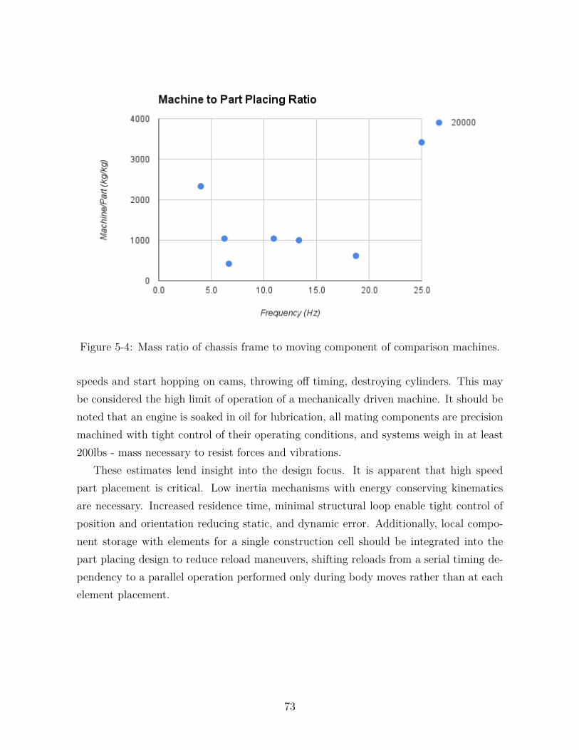
Figure 5-4: Mass ratio of chassis frame to moving component of comparison machines.

speeds and start hopping on cams, throwing off timing, destroying cylinders. This may

be considered the high limit of operation of a mechanically driven machine. It should be

noted that an engine is soaked in oil for lubrication, all mating components are precision

machined with tight control of their operating conditions, and systems weigh in at least

200lbs - mass necessary to resist forces and vibrations.

These estimates lend insight into the design focus. It is apparent that high speed

part placement is critical. Low inertia mechanisms with energy conserving kinematics

are necessary. Increased residence time, minimal structural loop enable tight control of

position and orientation reducing static, and dynamic error. Additionally, local compo-

nent storage with elements for a single construction cell should be integrated into the

part placing design to reduce reload maneuvers, shifting reloads from a serial timing de-

pendency to a parallel operation performed only during body moves rather than at each

element placement.

73

Chapter 6

Implementation

The reader has now journeyed through a handful of chapters that introduce fundamen-

tal concepts crucial to the understanding of the design challenges of building relative

robotic assemblers of discrete cellular lattices. In the following chapter I will explain

how I applied that information directly to solving the problem of attempting to build

a robot that robustly and rapidly assembles non-stochastic, discrete, periodic, cellular

lattices. A number of mechanical design experiments were performed along the way to

understand the limits to inter and intracellular joining techniques, and limitations. Lat-

tice geometries were similarly explored, as node connectivity of course defines real estate

available for load transmission and fastening. Both the interface and lattice then define

trajectory requirements for an end-effector. Finally, a controlled experiment was per-

formed to compare a global referenced versus a local referenced assembler. The results

were evaluated against a system error budget and applied to inform new design direc-

tions. Simulations of new assemblers that implement learnings from the experiments and

analysis were constructed and are promoted as future build directions.

6.1 Geometries: Elements and their Interfaces

The design of the interface between discrete cellular lattice elements is the single most

critical element to the entire construction system. Struts simply bear axial load, but

the joint must transfer load in compression, tension, shear, couple moments, while also

providing alignment features that tolerate the stack up of error from both static and

dynamic loading conditions contributed to by both the lattice, and the assembler (§4). In

a preference towards structural rigidity the joints would be permanently fixed, and fused

75

of the same material as the struts to allow a simple, continuous load path, with minimal

stress concentrators. In preference toward rapid assembly rates the nodes would passively

align themselves, at some distance, perhaps with an attraction field (magnets are used

in self-assembly modular robotics), such that the parts could essentially be ballistically

fired at high rate in the general direction of the lattice, and would non-stochastically

self-assemble into their specified location, without error.

The reality is, the solution is a balance of each of the design requirements, founded

in engineering first principles. The premise of the preceding chapters has been to layout

the foundational concepts that constrain this design problem. As with many engineering

problems the process is iterative. Each feature is interdependent with its neighbor. Until

the robot is built it is not clear how much dimensional uncertainty due to static and dy-

namic errors will need to be managed by the joint. The kinematics of the robot, cannot

be settled until a lattice is identified to be constructed with an element type that can be

secured with a joint that satisfies the requirements of load transfer, error management,

minimal post fastening requirements (pins, screws, etc.), and high packing density. Not

all of these, though, must be solved simultaneously. In reality the primary dependency

is identifying a node interface that can be placed with minimal precision, yet self-locates

with enough positional certainty for the next element to be placed in its required ad-

jacent position, transmits loads uniformly, and builds a specified lattice topology. The

necessary trajectory profiles can then be determined, enabling the kinematic design of

the assembler. From this, initial prototypes may be implemented, and from there neces-

sary additional complexity can be added. Each of these primary constraints are based

on the premises of minimal structural loop, minimal moving mass, maximum stiffness,

and passive alignment. The design space can be narrowed rapidly once the fundamental

dependencies are understood:

∙ A construction system of non-stochastic discrete cellular lattices assembly .

∙ Maximize the stiffness to density ratio of final material in the ultra-light stiffness

regime.

∙ Maximize assembly rates.

∙ Assembled from discrete, reconfigurable parts.

∙ Minimize the packed to unpacked density ratio.

∙ Manufacture with scalable manufacturing processes.

In order to maximize the stiffness in the ultra-light regime a highly triangulated lattice

was implemented [32]. The maximum stiffness to density comes from exactly constrained

76

sub-structures so that there is no added mass from redundant, indeterminate supports.

In order to maximize assembly rate elements need to passively orient into their final

positions precisely, stiff, and constrained. Similarly, as the assembler translates across

the structure it must itself passively align with the lattice, repeatably, and minimize

high-frequency motions of inertial components while keeping degrees of freedom to a

minimum.

6.1.1 Building Blocks

It was learned that the only rigid, regular, closed-cell polyhedra that fill space are the

tetrahedron, and the octahedron. To maximize stiffness for an isotropic cellular material

only rigid closed-cell polyhedra should be used to avoid multi-phase mixing of rigid

(stretch-dominated), and non-rigid (bending-dominated) cells [35]. Alternative design

configurations could be generated with multi-phase mixtures producing orthotropic or

quasi-orthotropic properties that may have greater sparsity, and higher specific stiffness

in particular loading directions. The takeaway though is that the load bearing structure

is the tetrahedron and the octahedron, and thus should be the focus of examination.1

Some questions arising around the order of operations of assembly inform decisions

about minimum construction features: if a cell is to be placed adjacent to an already

fixed cell, whose nodes retain the locational information; must their orientations be

indexed? Should the lattice be discretized all the way down to the placement of individual

nodes, and struts, or should there be some minimal functional element from which to

construct? Figure 6-1 demonstrates a construction method utilizing only distance, and

node elements. Two concepts become apparent: a large number of degrees of freedom

are necessary to assemble even the simplest single structural element - the triangle, and

it becomes unclear where the boundary exists between cells. This then scores poorly on

the assembly kinematic scale, and requires a more optimal solution.

The structural component is defined as a closed cell, regular, rigid, polyhedra voxel.

In the case of the octahedron there are twelve struts, eight faces, and six nodes. The

struts, and nodes are the load bearing components. The elements can be assembled to

form voxel cells, which are then placed into the lattice; or, the elements can be placed

independently, sequentially, or simultaneously to form the polyhedron. I realized though,

1This is an important realization as the inspiration for this research was initiated from the x-shapeelement of the cubic-octahedron specified by Cheung [17]. More specifically, the cuboct are vertexconnected octahedra formed from an X-shape design (figure 6-11) that require the placement (andinterweaving) of ten elements before managing to construct a single constrained structural element.

77

Figure 6-1: Distance, and angle constraint assembly process. Three degrees of freedomare necessary to form each closed triangular truss-face. Each truss face must then becircularly arrayed three times and mirrored about their base plane to form an octahedron;a large number of degrees of freedom are necessary to construct with individual strutelements.

that because the triangle is a minimal structure to constrain points in two-dimensional

space, and that because I want to build the structural elements directly, and rapidly,

then it must be that the optimal solution to those design constraints is prefabrication of

structural triangles, and direct placement of them into cells. In this way the assembler

may place the maximum amount of structure with minimum effort simultaneously, while

retaining high packing density with a mostly planar discrete element.

The triangle can be combined into any number of geometric cell shapes which when

repeatedly patterned, or tiled, form rigid or deformable lattice structures. A single, tri-

angular, nearly planar part type assembles to form the four faces of a tetrahedron or the

eight faces of an octahedron, or other triangulated geometries (figure 6-2). The repeated

tiling of these geometries form lattice structures whose global stiffness properties are

dependent on the relative orientation of the triangular enclosed volumes, and the con-

nectivity of struts between the nodes of the triangles. In this manner rigid or deformable

lattice structures may be constructed from a simple, yet, structural element. Then, it

becomes the job of the vertex geometry to define what specific orientations are allowable.

In this way, the triangle bears the load, while the interface at the node (vertex) embeds

functional information directly into the structure.

78

(b)(a)

Figure 6-2: Node-to-node connections possible with (a)vertex-connected and (b)face-connected lattice topologies. In (b) an interface geometry attempts at passive kinematicalignment: intracellular interface is ball and cone, while intercellular are tapered faces;both rely on a shear pin for tensile load. (Dimensions are 100mm node-to-node in bothframes.)

6.1.2 Interfaces

Figure 6-3: An alignment feature that has Þ polar periodic symmetry, allows more thana millimeter of deviation in all degrees of freedom and self-energizes in compression (gridsize is 1cm). The broad face, and interlocking nature of the joint enable moment couplingacross the interface.

The node defines the functionality of the lattice, but how are elements and cells fixed

together, and, by what means? Directly building the structural blocks leads the analysis

to consider two joint types: intracellular, and intercellular interfaces. A large variety of

instantiations of kinematic alignment features, and combination intra/intercellular inter-

faces were designed and evaluated, primarily focused around node-to-node configurations2. If bending conditions exist due to lattice geometry, the node must couple moments

2At first glance (fig. 3-8), a lattice topology of node-to-node connections appears non-optimal

79

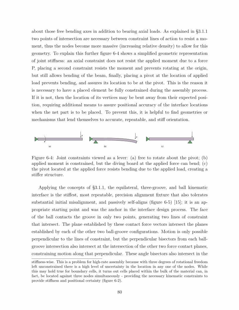
about those free bending axes in addition to bearing axial loads. As explained in §3.1.1

two points of intersection are necessary between constraint lines of action to resist a mo-

ment, thus the nodes become more massive (increasing relative density) to allow for this

geometry. To explain this further figure 6-4 shows a simplified geometric representation

of joint stiffness: an axial constraint does not resist the applied moment due to a force

P, placing a second constraint resists the moment and prevents rotating at the origin,

but still allows bending of the beam, finally, placing a pivot at the location of applied

load prevents bending, and assures its location to be at the pivot. This is the reason it

is necessary to have a placed element be fully constrained during the assembly process.

If it is not, then the location of its vertices may be bent away from their expected posi-

tion, requiring additional means to assure positional accuracy of the interface locations

when the net part is to be placed. To prevent this, it is helpful to find geometries or

mechanisms that lend themselves to accurate, repeatable, and stiff orientation.

PP

(a) (b) (c)

Figure 6-4: Joint constraints viewed as a lever: (a) free to rotate about the pivot; (b)applied moment is constrained, but the diving board at the applied force can bend; (c)the pivot located at the applied force resists bending due to the applied load, creating astiffer structure.

Applying the concepts of §3.1.1, the equilateral, three-groove, and ball kinematic

interface is the stiffest, most repeatable, precision alignment fixture that also tolerates

substantial initial misalignment, and passively self-aligns (figure 6-5) [15]; it is an ap-

propriate starting point and was the anchor in the interface design process. The face

of the ball contacts the groove in only two points, generating two lines of constraint

that intersect. The plane established by these contact force vectors intersect the planes

established by each of the other two ball-groove configurations. Motion is only possible

perpendicular to the lines of constraint, but the perpendicular bisectors from each ball-

groove intersection also intersect at the intersection of the other two force contact planes,

constraining motion along that perpendicular. These angle bisectors also intersect in the

stiffness-wise. This is a problem for high-rate assembly because with three degrees of rotational freedomleft unconstrained there is a high level of uncertainty in the location in any one of the nodes. Whilethis may hold true for boundary cells, it turns out cells placed within the bulk of the material can, infact, be located against three nodes simultaneously - providing the necessary kinematic constraints toprovide stiffness and positional certainty (figure 6-2).

80

Figure 6-5: On the left is a standard issue three-groove kinematic coupling [15]."For goodstability in a three-groove kinematic coupling, the normals to the planes containing thecontact force vectors should bisect the angles between the balls."[16]

centroid at the coupling centroid. The virtual center point established at the coupling

moments that are external to the frame actually provide a rigid moment arm that is larger

than the frame, anchored at each virtual center point. Thus, this equilateral structure is

isometrically stiff [16].3

The concepts of separated constraint line intersection turn out to apply to not only

nodal interface design, but also help to define how lattice topology affects stiffness. Kine-

matic constraint was utilized, or inspired a number of design studies, some shown below.

It was found that it was also pivotal to the development of one lattice topology in par-

ticular, helping to define not only its lattice stability, and interface design (§6.2.1), but

also was implemented by the trajectory requirements of the automated assembler that

was simulated (6.3.6).

(a) (b)

Figure 6-6: (a) flat elements (PF1) with alignment features; (b) interlocking joint withadditional complexity (OH5).

3This behavior is also seen in angular contact bearings, which when arranged in duplex demonstratehigh stiffness to moment loads due to the high contact angle (often 20-45 degrees) projecting virtualcoupling moments external the their own frame.

81

6.2 Geometries: Lattice Topologies

Overall structural performance is highly dependent on the geometry of the lattice; scala-

bility is dependent on affinity for robust attachment between individual elements; assem-

bly is dependent on the three R’s: repeatable, robust, and rapid. Simplicity is a primary

design anchor as it relates directly to packing density as well as manufacturability; it

favors parts from flat-stock that readily stack like the stock from which they are formed.

Yet, repeatable rapid assembly tends to favor greater feature complexity at the node to

manage misalignment. Each tiling geometry has specific, discrete, sets of orientation,

that define the level of constraint of assembled, and partially assembled cells, along with

the kinematic trajectory requirements for placement of the individual elements. Under

constrained elements have indeterminate free nodal locations, introducing significant un-

certainty to the assembly process. As seen in §4.2.2 error bounds cycle rates; constraint

directly affects the rapidity of assembly. Coordination number also drives nodal com-

plexity, with increasing connectivity demanding increasingly more physical real-estate at

the node, decreasing mass efficiency of the architecture.

Below is a sampling of some lattice geometries that were evaluated, followed by a

more in depth description of the lattice interface development, and how the principles

were applied.

6.2.1 Face Connected Octahedra

The face connected octahedra lattice has a coordination number of Z=6, it is an exactly

constrained topology. The even number of edges of an octahedron enable it to be formed

from just four regular triangular faces. The edges are the load bearing members of

the octahedron. So an equilateral triangular component can be created by extruding

members centered along the ideal edges of the triangle. Rather than building separate

edge elements, three edges, and respective nodes can be produced simultaneously. This

triangular element type allows the formation of the twelve edges of an octahedron with

only three or four elements, depending on the desired configuration. Both configurations

mirror triangular elements across their vertices forming octahedra from the edges of

four faces. The faces themselves may be defined as open or closed. Figure 6-2 shows

these two different lattice topologies, each constructed from four, or three face elements.

One configuration of four triangular bits allows vertex connected octahedra - the cubic

octahedron. Another configuration exists of three elements mirrored across vertices,

82

arranged into a partially formed octahedron that is then stacked face-to-face with a

neighboring octahedron. The edges from the shared face are shared to close the next

octahedron.

This shared face arrangement, and column stacking of octahedra defines a bi-directional,

cross-linked, triple helix column where each vertex is exactly constrained by six edges.

This triple helix resembles the structure of collagen with high connectivity between the

helices. The entire helix is formed from a single part type, or may also include an ad-

ditional fastening element. Multiple levels of complexity may be formed into the part

including using the central face as a location for additional functional components such

as sensors or actuators.

As it turns out, connecting regular octahedra face-to-face intersect three nodes from

each face, coordinating six non-collinear members to meet at each node. Each node

thus satisfies the modified Maxwell Criteria and is exactly constrained. Further, because

a face is shared and a π6

periodic lag exists, it is possible to borrow a set of edges

from the neighboring cell, producing octahedra with only three triangular elements, each

representing one face, and three nodes. More importantly though is that by projecting

the angle bisector normal to the mating face, a plane is formed whose normal at the

intersection point is a contact force vector that intersects the similar, and adjacent contact

force vector emanating from the other two corners of a shared triangular face. This means

an equilateral coupling tetrahedron forms external to each similarly arranged triangular

face, providing a stiff structure. Or, in other words, a triangular element can be designed

such that each of its nodes are exactly constrained and the element kinematically aligns

to its neighboring element.

The structure aligns well with the geometrical ideal with regards to stiffness, kine-

matics, as well as design for assembly. The nature of the interface is that a singly applied

nesting force orthogonal to the primary plane of the element evenly nests into the bound-

ary planes of its neighbors. A discrete interface was identified that again exploits the

polar periodicity of the octa-stack, whereby the node of the next element to be placed

loops around the previously placed nodes of two elements, locking into a fixed position.

The geometry of the interface aligns load paths to near ideal virtual nodes such that

load transmission across the joint closely retains the pin-joint assumption for stretch-

dominated behavior while maintaining a fully reversible interlock whose operation is

orthogonal to the load path (figure ??). Tapered interfaces tolerate some misalignment,

and passively orient themselves to a repeatable position. Finally, the nesting force vector

83

Figure 6-7: Kinematic constraints of the face connected octahedra lattice. (a) showscoupling triangles can form rigid coupling tetrahedra in 3d; (b) colored lines show the sixlines of constraint at each node provided by the alternating faces of stacked octahedra.

Figure 6-8: Close-up view of node interface for the octa-stack configuration.

is also the single degree of freedom necessary to assemble the part into the structure.

Single vector assembly simplifies the machinery of the robot by limiting kinematic

degrees of freedom, and potentially allows higher assembly rates by limiting unwarranted

inertially induced vibrations. With a lattice topology and a joint interface identified that

satisfy the primary design anchors the kinematics of an automated assembler that can

satisfy the interface assembly requirements can be evaluated. Due to the periodic nature

of this structure automation can be parallelized. A model of a potential robotic assembler,

technically referred to as the octahedral turret version six (OT6), and colloquially as

Leapfrog, is shown stepping through an assembly procedure in figure 6-22. Further

description of the robot is explained in §6.3.6.

84

70mm

Figure 6-9: Octahedra (blue) tile vertically face-to-face, and edge-to-edge laterally, withdipyramidal tetrahedra (magenta) filling intermediate volumes, and which again tile withthemselves on edge. Shown in rendering as well as discrete lattice.

70mm

Figure 6-10: Mechanical testing of octa-stack under position controlled loading. Themiddle image just before failure due to buckling. The right-most image is near totalfailure, half of the struts have already broken.

6.2.2 Vertex Connected Octahedra - Cuboct

The vertex connected octahedra lattice has a coordination number of Z=4. This claims it

has two rotational degrees of freedom. When the vertex-connected octahera lattice topol-

ogy is approached from both the Hashin-Shtrickman approach of multi-phase mixtures

§3.1.5, and the modified Maxwell criteria from Pellegrino §3.1.2, they both suggest this

lattice structure is not isotropically rigid, but instead should express bending dominated

behavior in shear loading conditions. The easiest way to describe the HS mixture is that

a mixture of rigid and bendable forms will perform as ratio of the relative mixture of

those volumes. This structure has also been referred to as the cubic octahedron (cuboct),

and it is that description that helps see the bending dominated nature. Figure 3-6 shows

85

the two different closed-cell polyhedra contributions to the structure. The blue are the

rigid octahedra, the magenta is the cuboct. The cuboct is clearly non-rigid by Maxwell’s

criteria, loads applied to any face cause the polyhedra to act as a mechanism and com-

press. Looking at figure 3-4 shows the top half of a cuboct structure, and again, shows

how there is mobility in the structure.

Yet, despite these three strong arguments for the cuboct to be bending dominated in

shear, I propose there is actually a condition where the structure is rigid in shear. In a

condition where top and bottom interfaces are cemented into a plane, and shear is applied,

the structure is again stiff. This can possibly be understood by two means: one by

Deshpande et al. explanation of boundary conditions as part of the multi-phase mixture

[35], and second by principal stress analysis. Normally, I would expect a shear load to

cause a four-bar linkage type of mechanism to be expressed; alternating expanding, and

contracting distances between nodes. By constraining the upper and lower boundaries,

however, such that the nodes cannot change their relational distance, and cannot move

in the y-direction the end condition struts have then reduced their degrees of freedom.

The applied shear load is then a pure shear load with zero x or y stress contributions.

This can be seen in the following equations [44]:

àn =1

2(àx + ày) +

1

2(àx ⊗ ày) cos 2� + áxy sin 2� (6.1)

àn = áxy (6.2)

where, àn is principal stress, àx,ày are x,y coordinates of stress, and áxy is shear in the

xy plane. This shows that when a material is loaded in pure shear, the principal axis of

stress is aligned along the ��/4 direction. In that case, the principal stress is then aligned

directly along the struts, providing again, pure axial loading of the struts, thus, providing

a stiff, and strong structure. So, in this loading condition, it may be that in fact, as it

was shown this lattice topology is the lightest stiffest structure in the ultralight regime

[17]. This conclusion remains funny in my mind as I can visualize how a direct forty-five

strand should take all of the stress of shear, and yet the void phase is a pure mechanism.

Perhaps the question still remains, is this loading condition something to be expected

in the wild, or is it a convenience of numerical evaluation? This topic is perhaps worth

further examination at a future date.

The element design described by Cheung was composed of x-shaped elements arranged

in-plane and orthogonal to one another, the ends of the X meeting at the midpoint of

86

the orthogonal X. The assembly strategy relied on bending and weaving parts into place

and a tight dimensional fit to restrict motion and finally fastened with an additional

shear pin. A model of this is shown in figure 6-11 (a). I immediately discounted this

assembly strategy for the following reasons: first weaving parts from multiple directions

would require dexterity, tight tolerance fitting is difficult for robots, and finally the free

ends introduce uncertainty for placement.

To manage the free end condition I investigated closed curve base elements such as

the square, and the triangle, and how they could be made to incorporate alignment

features, figure 6-11 (b), and (c) show these respectively. The square-element provides

wide face-face interfaces to allow passive alignment from the orthogonal oriented corners,

but requires a clip to tie together the embedded pins. The triangle shape of (c) was

the beginning of exploration into constructing the octahedron directly with triangular

faces, rather than laying out unneccesary periphery edges. Details of the interface are

also visible in (a) from figure 6-6, tabs help with axial alignment and the joint is fastened

by compression with a custom designed plug that is transparent in the image. Further

investigations included triangular shapes with more complex passive alignment geometry

and dual interfaces such as those in figures 6-2, 6-6.

As seen in those figures, the cell geometry does, as it turns out, lend itself to single axis

assembly with the potential for kinematic alignment features. Progress in this direction

had been detoured as at the time the face-connected, triple-helix configuration emerged

as a promising direction that tied together many facets of the design requirements. The

vertex connected structure may return for future research initiatives.

100mm 100mm(a) (b) (c)

Figure 6-11: Cubic-octahedron, or vertex connected octahedra: (a) x-shape elementdesign with shearpin; (b) square-element with clipped pins; (c) triangle-element withinterlocking fingers.

87

Figure 6-12: Edge connected octahedra with kinematic constraints colored (image credit:Ben Jenett)

6.2.3 Edge Connected Octahedra

The edge connected octahedra has Z = 6, it is exactly constrained. This configuration

allows the construction of voxels which when placed are always fully constrained. This

is a viable construction topology and was used as the basis for the first full assembler

system built, figure 6-14. The interface design relied on snap fit joints requiring 70N of

applied force to sufficiently engage. The removal of the cells again required 70N force, or

additional actuation to help open the snaps to allow disengagement (performed by grad

students with tweezers).

6.2.4 Kelvin

70mm

Figure 6-13: Kelvin Lattice, standard discrete - left, and with reduced degrees of freedom,right. (node-to-node spacing is 100mm)

The Kelvin lattice has a coordination number Z = 3. There are four non-collinear

struts entering into a node, two pairs each operating along the same plane. This leaves

three rotational degrees of freedom. Some attempts have been made to increase the

rigidity of the structure by introducing an additional strut to the element as seen in

88

figure 6-13, making it a reinforced Kelvin lattice. However, the rotational degrees of

freedom remain, regardless. The specific stiffness may be increased alongthe direction of

the newly added strut, as the element is itself now stiff, however the rotational degrees of

freedom cannot be constrained and as such the system operates in bending in all other

modes than direct compression along this specific orientation.

From the point of view of assembly this structure receives low grades for its high level

of mobility. The nodes do not naturally resist bending, so they either must be oversized to

couple the moment, else the position of the free nodes of that element are indeterminate.

For relative assembly the structure provides an even worse operating condition, because,

even in complete, closed polyhedra form it expresses many degrees of freedom; essentially

this structure acts as a trampoline for a locally referencing, relative robotic assembler.

6.3 Robots: Designs toward dB Scaling

The studies above lend insight into the design focus, and help shape a strategy to assure

robust, rapid assembly of discrete cellular lattices. The periodic nature of the lattice

provides a structured environment in which an assembler can to be tuned to operate. The

level of discretization and topology of the lattice affect the kinematic requirements of the

assembler. Based on what has already been learned it is apparent that part placement and

locomotion require minimal dwell time. Low inertia mechanisms with energy conserving,

and minimal vibration inducing kinematics are necessary. Local component storage can

reduce reload maneuvers. Further, shifting reloads from a serial timing dependency to

a parallel operation performed as part of body moves rather than as discrete events can

potentially lead to time savings. Most importantly though, it has already been shown

that joint interfaces which reduce assembly precision requirements enable higher speed

operation by way of reduced dwell to wait for settling of dynamic errors. A successful

discrete lattice assembler system integrates the design of the lattice with that of the

assembler, sharing precision and parallel mechanism across lattice and machine.

While designs had already been developed informed by the constraint and tolerance

studies, discussed in previous chapters, a controlled experiment was performed to demon-

strate the need for these specific system integrations. The following outlines what I built,

tested and sketches of what is planned to be built in order to reach super-hertz assembly

rates for digital lattice materials.

89

6.3.1 Gantry-based

70

Figure 6-14: The gantry-based relative robotic assembler (designed and built in March2015). Also shown with error budget coordinate transformations in figure 4-2.

To test the dependencies of discrete lattice assembly I built a custom, relative robotic

assembler to test against an off-the-shelf, traditional, linear kinematic, gantry-type CNC

machine (a Shopbot PRS Alpha). The question asked was: does an assembler that locally

references a lattice, place with more or less precision than a globally referenced assembler?

The experiment consisted of picking up an octahedron voxel from one location, and then

placing it into a target position within an edge-connected octahedral lattice. The two

machines had the same kinematic configuration consisting of linear actuators for x, y,

and z axes. The dependent variable being that the custom built assembler system was

mounted directly on the lattice by way of an incremental relative motion system which

included leg, and foot actuators.

A custom gantry-type of robot (figure 6-14), similar to a traditional computer numer-

ically controlled (CNC) router was built to evaluate a traditional manufacturing platform

as a means of assembly. The control machine to evaluate against was a ShopBot PRS

Alpha, a design that consists of a long x-axis with an overhead gantry y-axis, both driven

by rack and pinion actuators. The traditional machine is considered a global coordinate

frame system because all moves and actions are done with reference to a single refer-

ence frame established at some static position on the machine. The relative robot has

been considered a local coordinate frame machine because it incrementally steps along

the lattice, referencing its position from the local cells, and placing components relative

to this non-static local coordinate frame. The custom assembler consisted of a similar

90

structural loop as the traditional machine including a linear x-axis, and a linear overhead

gantry, but also include additional x, and z axes for a locomotion system. In this way,

the custom router became a robot able to take discrete steps across the lattice, and then,

in an analog fashion, place a set of cells within its local work area.

The gantry system fabrication was performed primarily by myself, and included CNC

machining, fused deposition manufacturing, lasers, wire-edm, and waterjet processes.

The chassis was machined from aluminum billet on a 3-axis CNC machining center.

The remaining aluminum components were machined on a 5-axis CNC mill or waterjet.

The lattice elements and the end effector were constructed of laser-cut acetal. The feet

(Ben Jenett) and the foot actuator mounts were FDM, and waterjet. The actuators

make use of precision linear guideways for tracking. Three varieties of actuators were

designed as separate test cases: belt drive, capstan drive, and rack-pinion. The rack

tooth-profile were precision machined on a wire-EDM (with the help of Will Langford

and Sam Calisch), and their chassis machined of delrin. The drive systems were stepper

motors on the x, y and secondary y axes. The z-axis actuators were all driven by brushed

dc gear-motors. The control system was implemented with an off-the-shelf TinyG stepper

motor controller [68]. A hack was performed to allow the TinyG to communicate with

the DC motor actuators (hacked by Sam Calish, Will Langford, Amanda Ghassaei). This

is the complete system that I designed, and built with help from my fellow labmates.

This system placed cells on a time scale on the order of 0.1Hz.

The experiment consisted of placing octahedral cells into an edge-connected lattice

topology. The cells were preformed from laser cut delrin elements. The interface of

the edge-connected octahedra cell type used in the gantry robot experiments (shown

below the gantry assembler in figure 6-14 and 6-12 were designed to include an inte-

grated flexural snap. The force required to engage the snap interface was 70N. The

manufacturing tolerance of the laser used to manufacture the elemetns holds to about

0.003” ≡ 0.05��. The interface had a gap designed to utilize the kerf of the laser process

of 0.004” ≡ 0.15�� for a total of 0.3�� allowable variation in parts placement.

Initial experiments were performed to compare the performance of the global reference

frame system to the locally referencing relative robotic assembler. In this experiment

cells were picked up from a hopper, and placed onto a static positioned lattice. The PRS

Alpha claims a positional accuracy of ∘0.002”. Evaluating the structural error loop,

including a 1.5à coefficient required a gap of 0.23��. Including the positional accuracy

of the machine brought the required interface gap of 0.279��. A second experiment was

91

performed with the relative robotic assembler of similar gantry-type design (figure 6-14).

Following the protocol of the first test, the cells, preformed from flat, laser-cut elements,

were stored locally, in a hopper type of fixture, on the machine. The assembler, this time

though, was mounted directly onto the lattice. In both tests the end-effector was used

to zero the machine origin to the target position. The task performed included picking

up, and then placing cells into a target position on the lattice.

The first tests on the global reference system (ShopBot)were successful in placing

parts. The tests performed with the relative robot did not successfully, repeatably place

parts. An error budget analysis of the two systems lends insight to the difference in

placement results. An example analysis of the total error budget of the custom relative

robot, as described in §4.1.2, due to the structural loop in figure 4-2 of one serial path

from the leading foot to a cell placement was evaluated. The calculation was performed

with the assumption of no angular misalignment and manufacturing error on the order

of 0.05�� per part - reasonable for machined components.4 In this case six coordinate

frames5 were implemented with the homogeneous transformation matrix method of calcu-

lating the total error budget (§4.1.2) of the robot chassis side, and similarly included the

contribution of the five lattices located between the target origin, and foot in question.

The error from each structure, and lattice are below. An error of 0.25�� is contributed

structurally, and a 0.15�� error is contributed from the lattice. Applying the 1.5à from

§4.1.1, this analysis leads to to a necessary joint clearance of ∘0.44��.

︀

︀

︀

︀

︀

︀

︀

︀

Ósx

Ósy

Ósz

1

︀

⎥

⎥

⎥

⎥

⎥

⎥

︀

=

︀

︀

︀

︀

︀

︀

︀

︀

0.25

0.25

0.25

1

︀

⎥

⎥

⎥

⎥

⎥

⎥

︀

,

︀

︀

︀

︀

︀

︀

︀

︀

Ólx

Óly

Ólz

1

︀

⎥

⎥

⎥

⎥

⎥

⎥

︀

=

︀

︀

︀

︀

︀

︀

︀

︀

0.15

0.15

0.15

1

︀

⎥

⎥

⎥

⎥

⎥

⎥

︀

(6.3)

àgap = às + àl = 0.4�� (6.4)

where, às is the structural error, and àl is the lattice error contribution. The individual

cell interface was designed to accommodate up to 0.3mm of variation. The global ref-

erence system with a structural loop error stack of 0.28mm did manage to place parts.

The local reference system with a structural loop error stack of 0.4mm did not manage to

place parts. The global frame system has consistent control of its structural loop, while

4The reason for a milled aluminum chassis was exactly this point. In order to have a fair comparisonbetween machines rigidity, and precision was desired, two properties currently difficult to achieve withoutmachining.

5In reality, there are a great more number of component interfaces that would need to be accounted.

92

the local system must managed the error contribution of all of the discrete elements

between its target position and its locomotion system. Further, the dynamics timing

analysis shows that if an allowable settling error of 0.1mm is allowed, and an operational

frequency matched to the MIT Cheetah robot is desired (4 Hz) then moving mass must

be limited to a mere 0.005kg.6

An interesting note from the experiment is that it was immediately apparent that the

error contribution from standing on the lattice was significant when it was attempted

to zero the robot to the origin. It was not possible to establish a mutually agreed upon

origin between teh lattice and the chassis of the robot. If an origin was chosen on the

lattice then retrieving a cell from the local hopper was not successful. If the origin was

chosen to pickup the cell from the local hopper then there was not success with fully

engaging the cell into the lattice snaps. The results of the experiment showed, that due

to the increase in uncertainty from the dimensional variability accumulated from the

lattice elements, a local assembler must actually be a locally global assembler - that is

the lattice should not be part of the structural loop during assembly.

Figure 6-15: Maximum frequency of operation with an axially loaded aluminum beamas an end-effector.

6One might question, how does the MIT Cheetah reach such high speed operation with presumablygreater mass? The answer is two fold: for one, there is great attention to reduction of mass and inertiaof the moving components, the actuators are mounted in the body and light-weight linkage mechanismsare used to keep mass low, second, exact foot placement precision is not required, rather their concernis velocity profile and foot orientation during the stance phase of locomotion [67].

93

The takeaway from this experiment is that a traditional manufacturing kinematic

assembly strategy is not adequate for automated relative lattice placement. If dynamic

error were also included in the analysis, a wider gap would be necessary, minimizing the

effectiveness of a snap interface. The design of the interface defines if successful assembly

is even possible, and then what rates may be achieved. A relative robotic assembler

requires a more integrated design approach, where kinematics, structural loop, and joint

topology are iteratively designed together; primarily the assembly process must mini-

mize the structural loop. The global assembler was more successful in the experiment

because the tolerance stack-up through the structural loop only ever included its own,

tightly controlled, and non-variable, hardware - it did not rely on the error contribution

from a multitude of discrete cells in the lattice. In order for a robotic assembler that

moves relative to the lattice to assemble locally, the assembler must minimize its struc-

tural loop; the assembler must place parts only relative to itself, without dependency

on non-adjacent lattice elements. At each incremental step the assembler must consider

that location its instantaneous origin, and place adjacent elements with reference to only

this instantaneous coordinate frame. In this way, static dimensional uncertainty is re-

duced, allowing more room to manage the positional variability from dynamic conditions,

thereby potential enabling faster assembly rates.

6.3.2 Mandrel-based

The mandrel-based assembler was a study in dimensional control during cell construc-

tion. Learning from the data in table 5.1, the performance of placing individual elements

is speed-limited due to the need to retrieve and place individual components onto a not-

yet fully constrained lattice. This system utilizes the square-shape element to construct

cuboct cells. A mandrel is a fixture that temporarily defines the location of components

during subassembly procedures, which is then removed from the final part post process-

ing. The system in figure 6-17 uses a mandrel to locally build a cell in the immediate

vicinity of the material handling system, and then place the completed cell onto the

lattice. This creates greater certainty, and stiffness during cell builds due to a short,

and high rigidity structural loop allowing a more robust, and faster assembly strategy.

Simple motion paths, and short traverse distances reduce vibrations while shortening

cycle times. Tighter control at part placement also reduces the need for joint complex-

ity, saving mass and cost. Locomotion, however, is a completely separate mechanism

from part placement. It implements the elastic averaging strategy to gain precision from

94

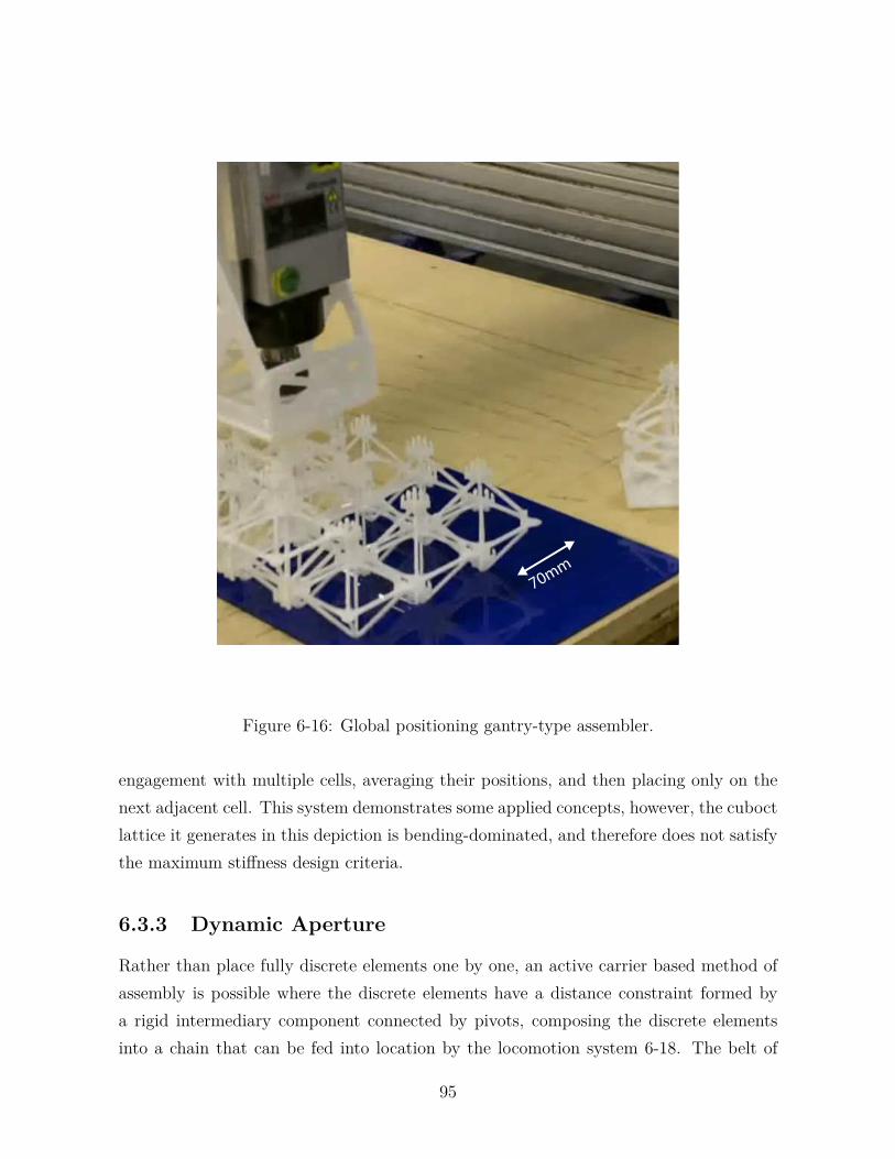
70mm

Figure 6-16: Global positioning gantry-type assembler.

engagement with multiple cells, averaging their positions, and then placing only on the

next adjacent cell. This system demonstrates some applied concepts, however, the cuboct

lattice it generates in this depiction is bending-dominated, and therefore does not satisfy

the maximum stiffness design criteria.

6.3.3 Dynamic Aperture

Rather than place fully discrete elements one by one, an active carrier based method of

assembly is possible where the discrete elements have a distance constraint formed by

a rigid intermediary component connected by pivots, composing the discrete elements

into a chain that can be fed into location by the locomotion system 6-18. The belt of

95

Figure 6-17: A mandrel based assembler. A mandrel provides a fixture for elements tobe placed onto before placement on the lattice assembly. Locomotion is then performedrelative to the structure. Code-name: Koala (cubes are 100mm edge to edge)

elements are stored either on rails, or in the figure shown folded into local hoppers, and

then they are fed into position by a rotary mandrel that creates a dynamic aperture. A

rack and pinion type of arrangement of rollers feeds the elements into the lattice, while

traversing along the lattice. The rigid elements pivot on their integrated carrier as they

roll along the rollers, similar to a chain on a sprocket. In this way both locomotion, and

part placement are integrated into the same mechanism.

The arrangement of adjacent rollers enables connecting the chains into volume en-

closing structures. Where total reconfigurability is lost in this case, due to the need for

specific lengths of carriers, speed of assembly is potentially gained. The rotary motion of

the rollers, similar to the bottling machine in §4.2, increase residence time with a no-slip

condition due to rolling (which just means the parts have no relative motion except for

with the target interface) providing a rigid, minimal structural loop with increased time to

fasten components without a reduction in linear velocity. The rotary motion also keeps

vibration low by providing a parts feeding trajectory with continuous non-interrupted

96

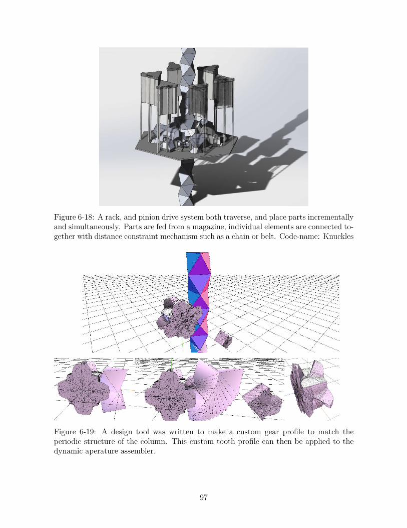
Figure 6-18: A rack, and pinion drive system both traverse, and place parts incrementallyand simultaneously. Parts are fed from a magazine, individual elements are connected to-gether with distance constraint mechanism such as a chain or belt. Code-name: Knuckles

Figure 6-19: A design tool was written to make a custom gear profile to match theperiodic structure of the column. This custom tooth profile can then be applied to thedynamic aperature assembler.

97

motions, essentially only the mass of the parts are making relative motions.

In an effort to build the rollers to truly match the part geometry a design tool was

developed, to build a custom gear profile that directly match arbitrary periodic surfaces.

Figure 6-19 shows some screen shots of the design tool operation 7. A round cylinder

is carved away by a single period of the tri-helix column (a double-stacked octahedron)

traced through an involute profile. By tuning the locomotion kinematics to the struc-

ture it is possible to minimize inertial costs, allowing lower vibration and higher speed

operations.

6.3.4 Fully Passive

Figure 6-20: The geometry of the assembly mandrel passively aligns elements duringplacement. Code-name: Zipper

A fully passive system was found 6-20 that uses a distance constraint, such as a carrier,

to time the zipping of elements into location . The geometry of the zipper provides the

necessary trajectory to fixture the joints between the elements. One degree of freedom is

necessary to traverse along the length of the column as parts are automatically fed, and

fixed into position. The joint operates in an inverse arrangement to that of the Leapfrog.

That is, the build direction is reversed and snap pins built into the structure provide

joint fixture, rather than being looped into position from the following set of cells.

A passive assembler relies on the three dimensional geometry of an assembly head,

or a mandrel, to define the path that the discrete element tracks along as it is placed

or removed from the lattice (figure 6-20). The discrete element follows along the path

7The design tool runs in HTML5 in the browser, and utilizes the javascript library Three.js.http://dma.cba.mit.edu/mechanical/jsTools/rackPinion/index.html

98

formed into the assembly head. Elements are fixed in place by the placement of the

following element. That is, the part is only fully constrained after the placement of

following adjoining parts. The trajectory necessary to mate part interfaces is iteratively

defined by the interface fixture geometry while it is itself, also, informed by the possible

trajectory (figure 6-21). Control of the timing for placement is defined by a distance

constraint between parts that are to be collinear in their placed configuration. The

distance constraint may be established by a carrier, such as a belt, cable or chain. In

this way the assembly system is similar to that of a zipper, where individual elements are

constrained by their neighbors in one direction, by a carrier in the opposite direction and

their assembly trajectory is defined by a physical track that the parts are pulled through.

The kinematics of this assembly strategy are that of a three-dimensional zipper. A single

degree of freedom is necessary to pull the zipper assembly head along the structure. This

degree of freedom may be actuated by external systems, or even the mass and inertia

of the motion of an initial seed assembly sequence, where gravity provides the constant

pulling force that drives the elements through the assembly head. The discrete elements

may be stored in a magazine, cartridge, reel or hopper type of system.

Figure 6-21: A passive mandrel type of assembly requires a distance constraint such asa belt or a chain between the components.

6.3.5 Hybrid Passive Dynamic

A likely candidate assembler design for building columns involves design features from

both the Zipper, Knuckles, and Leapfrog; the zipper assembler trades the carrier distance

constraint for a mechanical timing constraint. Discrete elements are timed, and fed into

location by the rack and pinion, while the geometry of the zipper assures trajectory

compliance. The rack and pinion also provide the single degree of freedom locomotion

mechanism. In this way the discrete elements require no carrier. The track still provides

the passive trajectory control while an active mechanism coordinates the dispersal of

99

discrete elements from their storage location and along the track. The latching may

be performed by tooth geometry, adhesion such as vacuum, magnetics, hook and loop,

adhesive bond, etc. Upon attachment of element to lattice the latch disengages. This

mechanism may also provide a locomotion system that traverses along the already formed

structure, such that the zipper is capable of self locomotion along the lattice. This system

provides a fully integrated, locomotion, material handling, and part placement strategy.

The integration of multiple systems reduce the serialized mechanism requirement to just

a couple of motions with potential timing characteristics outlined in table 6.1.



Retrieve element from magazine �em 120 msMove element to position �ep 120 msFasten element �ef 0 msTotal Time per part �et 240 msCell placing frequency �ft 4.2 Hz

Table 6.1: Timing estimates for both placing three elements of a cell, and simultaneouslytraversing to the next cell with a passive loading mandrel.

6.3.6 Tri-helix Locomotion Integrated

The tri-helix locomotion assembler, figure 6-22, integrates all of the concepts presented,

and is the definition of an incremental global coordinate frame robotic assembler. The

lattice structure this assembles is the face-connected tri-helix structure §6.2.1, which is

itself the product of the pivotal design concepts presented in the preceding chapters:

the elements kinematically align with themselves, establishing an exactly constrained,

isotropically stiff by the tetrahedral intersection of its coupling moment bisectors, flat-

packs and is manufacturable at scale. The structural loop of the system is reduced

to its core elements. The end-effector is the part placement, parts feeder, locomotion

system, and error correction mechanism. The end-effectors, or feet have features that

provide kinematic alignment with the other foot mechanisms, therefore passively locating,

and locking to each adjacent foot (each of which includes at least one or more repeating

mechanisms that latch together as they step along the lattice). The overall structural loop

for part placement, and locomotion is actually independent of the lattice structure, and

instead contained within a single set of mechanisms on-board the robot. All operations

happen internally, and in parallel rather than as separate external systems, and can be

100

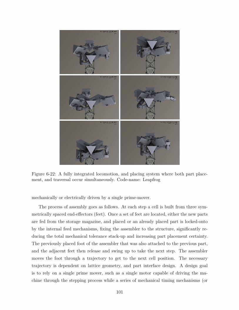
Figure 6-22: A fully integrated locomotion, and placing system where both part place-ment, and traversal occur simultaneously. Code-name: Leapfrog

mechanically or electrically driven by a single prime-mover.

The process of assembly goes as follows. At each step a cell is built from three sym-

metrically spaced end-effectors (feet). Once a set of feet are located, either the new parts

are fed from the storage magazine, and placed or an already placed part is locked-onto

by the internal feed mechanisms, fixing the assembler to the structure, significantly re-

ducing the total mechanical tolerance stack-up and increasing part placement certainty.

The previously placed foot of the assembler that was also attached to the previous part,

and the adjacent feet then release and swing up to take the next step. The assembler

moves the foot through a trajectory to get to the next cell position. The necessary

trajectory is dependent on lattice geometry, and part interface design. A design goal

is to rely on a single prime mover, such as a single motor capable of driving the ma-

chine through the stepping process while a series of mechanical timing mechanisms (or

101

electrically controlled) actuators drive the assembly, and locking chain of events.

The table 6.2 outlines design criteria specifications for placing components when sub-

systems are integrated together. Potential assembly rates of 1.5Hz may be possible with

a system of this nature. Faster operation may be possible, but the mass of the magazine

loaded with elements likely limits maximum acceptable assembly rates.



Retrieve element from magazine �em 25 msMove element to position �ep 75 msFasten element �ef 75 msTotal Time per part �et 175 ms

Lattice Locomotion - Foot

Unclasping foot mechanism �fu 100 msRaise foot assembly �fr 300 msClasp foot mechanism �fc 100 msTotal time to move foot �ft 500 msTotal time to build one lattice cell �ft 675 msCell placing frequency �ft 1.5 Hz

Table 6.2: Timing estimates for both placing three elements of a cell, and simultaneouslytraversing to the next cell.

This system is, in my mind, an accumulation of the knowledge so far developed in

this field of relative robotic assemblers of non-stochastic discrete cellular lattices. It

is a preferred direction of action going forward as it provides a data point for total

integration between lattice topology, and robotic assembler. While it does suffer from a

reciprocating, and rotating mass problem (as it currently swings a full magazine through

its locomotion trajectory), it is symmetrically balanced around the tri-helix axis, mutually

canceling induced vibrations. Development on this system is ongoing (figure 6-23), and

currently has a single cell assembly stage prototype near completion. This single-stage

system is designed to mount to a traditional robot arm (UR10 [69]) allowing the testing of

magazine, parts feeding, alignment and locking mechanism without the added complexity

of the locomotion system. In this way, individual components can be tried and switched

out with minimal risk or complexity to the system integration.

102

Figure 6-23: A prototype of the robot arm mounted single-stage integrated octahedralturret assembler(a collaboration between Matt Carney and Sebastian Nowak).

103

Chapter 7

Conclusions: Future Directions

The integration of the design of the interface between discrete elements, and robotic as-

sembler kinematics is of paramount concern to reaching high rates of assembly of robust

structural systems. The overall performance of the system comes down to the joints; how

much tolerance there is to misalignment scales assembly rates, and robustness of load

passing scales structural efficiency. Complexity at the joint costs mass, and creates: ob-

stacles for load paths, stress concentrations, and manufacturing complexity with reduced

packing density. Yet, joint complexity also reduces assembler complexity, and cycle times

by providing passive alignment features that reduce precision requirements. Addition-

ally, the structural loop of the assembler robot, and any reciprocating mass must be

minimized to reduce static, and dynamic uncertainty. The need for minimal uncertainty

in the structural loop leads to the concept of an incremental, or, instantaneous global

coordinate frame for relative assembler robots; the robot only ever places components

with respect to its own coordinate frame. The lattice cannot be part of the structural

loop, rather the robot attaches to the lattice, places a cell into its own alignment features,

then disengages, and increments to the next cell, leaving in place the just installed cell.

My research found that a gantry based relative coordinate frame assembler performed

more poorly than a similarly designed global frame system (§6.3.1). The reason is two-

fold: the relative gantry system must accommodate both its own long structural loop,

and that of the lattice, and yet does not exploit elastic-averaging (§4.1.3). The edge-to-

edge octahedral lattice interface provided minimal passive alignment features requiring

a total system precision of ⊘ ∘0.2��. The contribution to positional error from the

lattice consumed half of that allowable error. The manufacture of the assembler being

a combination of precision machined components, and imprecise fused deposition manu-

105

factured (3d printed) components limited its overall precision to an estimated 0.25mm.

While not quantified, there was additional error due to the control system, which in

the case of the assembler was operating in open-loop with stepper motors. While the

difference in machine, and allowable precision was slight, it was enough to prevent suc-

cessful assembly. Further, the dynamics of the gantry assembler would not be favorable

for high frequency assembly. Besides the speed limit of stepper motors, and the stiffness

of the machined aluminum chassis, and actuators, the substantial mass in motion would

provide significant limits to dynamic performance. Further, the motion paths required

to pick-and-place components were excessive requiring multi-degree of freedom traverses

across the full length of the chassis, costing time and/or power.

Relative robotic assemblers that incrementally traverse a lattice are not only feasible,

but, when their design is deeply integrated with lattice topology, they have the capacity

to operate at higher cycle rates than traditional serial-link configuration robotic arms, or

gantry-type configurations because of reduced mass, and traversal distances. Designing

lattices, and joints with simple kinematic trajectory requirements enable parallelization

of the assembly mechanisms while minimizing errant vibration. Co-location of element

storage with end-effectors reduce traverse distances. Geometry, such as mandrels, and

kinematic alignment features can help assert positional certainty - reducing dwell, and

settling times. The principles of elastic averaging can be utilized by locomotion systems

that span longer wavelengths than the cell geometry to increase effective local precision.

Alternatively, complete removal of the lattice structure from the incremental assembler

structural loop minimizes the error contribution from the lattice entirely.

For each of these improvements to be applied more assembly strategies must also be

evaluated, designed, built, and tested. While a few systems have been designed, and

prototyped, there are still many potential strategies for locomotion, or assembly. Rather

than a single robot assembling elements into voxels, and placing them, it may be that

voxel cells are assembled off-board, then, placed. Or, it is possible, assembly happens in

collaboration between multiple robots moving both inside, and outside of the structure.

The first next step is to gather the data point of an Instantaneous Global Coordinate

Frame (IGCF) assembler that removes the lattice from the assembly of the lattice. The

tri-helix (Leapfrog) system integrates all of the design concepts developed through the

research including the IGCF protocol. This machine is currently under development, and

should be completed to understand the implications of this concept. The learnings from

this will lead to future design efforts.

106

Future research might also further address new technologies at the interface. The

ultimate goal for reconfigurable interfaces is for a face-to-face element interface to exist

that operates as conveniently as a shared electron covalent-bond. An interface that

aligns with the assistance of a field active at some distance, can transmit tension as

well as compression, and moments, yet retains a continuous structural path would be

ideal. New material combinations that morph shape with changes in activation energy

could also potentially provide a robust reconfigurable interface. The design of struts,

and interfaces have much room for improvement. Current methods involved a brute

force design approach. Implementation of computational tools to further explore the

design-space of interfaces, and trajectories are of great interest. More detailed analysis

of buckling criteria, as well as strut material options will lead to designs with improved

cross-sectional second area moment of inertias to optimize stiffness, slenderness ratios,

limiting buckling in compression loading conditions. Finally, substantial dynamic analysis

of locomotion gaits, and system vibrations would enable the tuning of assembly systems.

RADCL would have significant societal impact on land, air, and space. Any construc-

tion process that starts with a foundation could utilize this technology by integrating the

periodically symmetric interface joints into the foundation. The RADCL systems would

begin construction directly from these foundational interfaces. Bridges are a primary

example of a system that would directly benefit from this technology. A foundation is

set, and a lattice construction of struts is built from pylon to pylon. With RADCL errors

could be corrected during the assembly process, or even later, inspection robots regularly

traversing the structure could pinpoint failures, and those sections directly deconstructed,

and repaired. This is in stark contrast to modern bridge construction techniques that

are not built for disassembly: for instance, the new construction of the eastern span of

the San Francisco Bay Bridge was found (after eleven years and $6.4 billion) to have

failed anchor bolts in the pylon that cannot be removed [70], posing safety concerns.

Other similar, but permanent construction such as that of dams, and levees could utilize

this technology to rapidly, and autonomously build more complex structurally conformal

reinforcing "re-bar" structures that would later be filled with concrete. In this case the

lattice is utilized for its best tensile properties while concrete provides the compressive

and fluid handling properties. Finally, large scale space structures such as large aperture

radio telescopes, solar arrays, or even new stations have not been realized as there has yet

been no scalable manufacturing process beyond unfurling. The RADCL system would

enable these technologies by autonomously assembling structures, incrementally increas-

107

ing their capacities as additional shipments of raw material arrive. Rather than build

deployable mechanisms that must survive launch vibration forces, shipments of discrete

elements optimized for mass, strength, and packing density would be shipped to space

flat-packed (minimally susceptibel to launch loads), and assembled into their final useful

forms by the RADCL systems.

Robotic assembly of discrete cellular lattices offers new opportunities for construction

of ultra-light stiff, and strong materials that are fully reconfigurable, and can be assembled

autonomously by relative robotic systems. There is a growing field of research around the

individual areas of non-stochastic periodic discrete cellular solids, and modular robotic

assemblers, yet the full integration of kinematic principles to drive the topology of the

discrete elements, and their autonomous assemblers has not yet been explicitly recog-

nized. The research performed here outlines the key design features necessary to realize

unbounded relative robotic assembly.

108

Bibliography

[1] KHS, “PET filler for still and carbonated beverages.”

[2] A. Menges and T. Schwinn, “Manufacturing Reciprocities,” Architectural Design,vol. 82, pp. 118–125, Mar. 2012.

[3] V. Zykov, P. Williams, N. Lassabe, and H. Lipson, “Molecubes Extended : Diversi-fying Capabilities of Open-Source Modular Robotics,” in IROS 2004, p. 12, 2004.

[4] P. J. Staritz, “Skyworker : A Robot for Assembly , Inspection and Maintenance ofLarge Scale Orbital Facilities,” in Proc of the 2001 IEEE, International Conferenceon Robotics and Automation., pp. 80–85, 2001.

[5] D. Hjelle and H. Lipson, “A Robotically Reconfigurable Truss,” in ASME/IFToMMInternational Conference on Reconfigurable Mechanisms and Robots (ReMAR), 2009.

[6] B. F. Nigl, S. Li, J. E. Blum, and H. Lipson, “Structure Reconfiguring Robots,”IEEE Robotics & Automation Magazine, no. September, pp. 60–71, 2013.

[7] K. C. Galloway, R. Jois, and M. Yim, “Factory Floor : A Robotically Reconfig-urable Construction Platform,” in IEEE International Conference on Robotics andAutomation, (Anchorage), pp. 2467–2472, 2010.

[8] R. Hoyt, “Dr. Rob Hoyt,” tech. rep., Tethers Unlimited, Inc., Bothel, WA, 2014.

[9] Wikipedia, “Aluminium foam sandwich,” Feb. 2015.

[10] K. A. Finnegan, Carbon fiber composite pyramidal lattice structures. PhD thesis,University of Virginia, 2007.

[11] W. K. Langford, Electronic Digital Materials. Master of science, MassachusettsInstitute of Technology, 2014.

[12] A. Ghassaei, “Digital Material Design Tool,” 2015.

[13] A. H. Slocum, Precision machine design. Dearborn, Michigan : Society of Manufac-turing Engineers, c1992., 1992.

[14] KHS, “Innofil Glass Capping Machine DRS-ZMS.”

109

[15] M. L. Culpepper, “Design of quasi-kinematic couplings,” Precision Engineering,vol. 28, pp. 338–357, July 2004.

[16] A. H. Slocum, “Design of three-groove kinematic couplings,” Precision Engineering,vol. 14, pp. 67–76, Apr. 1992.

[17] K. C. Cheung and N. Gershenfeld, “Reversibly assembled cellular composite mate-rials.,” Science (New York, N.Y.), vol. 341, pp. 1219–21, Sept. 2013.

[18] J. Ward, Additive Assembly of Digital Materials. PhD thesis, Massachusetts Instituteof Technology, 2010.

[19] S. E. Calisch, Physical finite elements. PhD thesis, Massachussets Institute of Tech-nology, 2014.

[20] G. A. Popescu, Digital materials for digital fabrication. PhD thesis, MassachussetsInstitute of Technology, 2007.

[21] J. J. Craig, Introduction to robotics : mechanics and control. Addison-Wesley se-ries in electrical and computer engineering. Control engineering, Reading, Mass. :Addison-Wesley, c1989., 1989.

[22] M. Yim, W.-M. Shen, B. Salemi, D. Rus, M. Moll, H. Lipson, E. Klavins, andG. S. Chirikjian, “Modular self-reconfigurable robot systems [grand challenges ofrobotics],” Robotics & Automation Magazine, IEEE, vol. 14, no. 1, pp. 43–52, 2007.

[23] K. C. Cheung, E. D. Demaine, J. R. Bachrach, and S. Griffith, “ProgrammableAssembly With Universally Foldable Strings (Moteins),” IEEE Transactions onRobotics, vol. 27, pp. 718–729, Aug. 2011.

[24] K. H. Petersen, R. Nagpal, and J. K. Werfel, “Termes: An autonomous robotic sys-tem for three-dimensional collective construction,” in Robotics: Science and SystemsConference VII, MIT Press, 2011.

[25] C. Detweiler, M. Vona, Y. Yoon, Seung-Kook Yun, and D. Rus, “Self-assemblingmobile linkages,” IEEE Robotics & Automation Magazine, vol. 14, pp. 45–55, Dec.2007.

[26] Y. Terada and S. Murata, “Modular stucture assembly using blackboard path plan-ning systems,” in International Symposium on Automation and Robotics in Con-struction, pp. 852–857, Citeseer, 2006.

[27] G. Theraulaz and E. Bonabeau, “Coordination in Distributed Building,” Science,vol. 269, pp. 686–688, Aug. 1995.

[28] K. Sugawara, N. Correll, and D. Reishus, “Object Transportation by Granular Con-vection Using Swarm Robots,” in Distributed autonomous robotic systems (M. AniHsieh and G. Chirikjian, eds.), vol. 104, pp. 135–147, Berlin, Heidelberg: SpringerBerlin Heidelberg, 2014.

110

[29] D. Lobo, H. Lipson, and D. A. Hjelle, “Reconfiguration algorithms for roboticallymanipulatable structures,” in ASME/IFToMM International Conference on Recon-figurable Mechanisms and Robots, pp. 13–22, IEEE, 2009.

[30] S.-k. Yun and D. Rus, “Optimal distributed planning for self assembly of modularmanipulators,” in 2008 IEEE/RSJ International Conference on Intelligent Robotsand Systems, pp. 1346–1352, IEEE, 2008.

[31] Y. Terada and S. Murata, “Automatic Modular Assembly System and its DistributedControl,” The International Journal of Robotics Research, vol. 27, pp. 445–462, Mar.2008.

[32] M. F. Ashby, “The properties of foams and lattices.,” Philosophical transactions.Series A, Mathematical, physical, and engineering sciences, vol. 364, pp. 15–30,Jan. 2006.

[33] R. E. M. Ashby M. F.; Medalist, “The Mechanical Properties of Cellular Solids,”Metallurgical Transactions, vol. 14, no. September, pp. 1755–1769, 1983.

[34] L. J. Gibson, “Biomechanics of cellular solids.,” Journal of biomechanics, vol. 38,pp. 377–99, Mar. 2005.

[35] V. Deshpande, M. Ashby, and N. Fleck, “Foam topology: bending versus stretchingdominated architectures,” Acta Materialia, vol. 49, pp. 1035–1040, Apr. 2001.

[36] Z. Hashin and S. Shtrikman, “A variational approach to the theory of the elasticbehaviour of multiphase materials,” Journal of the Mechanics and Physics of Solids,vol. 11, pp. 127–140, Mar. 1963.

[37] N. a. Fleck, V. S. Deshpande, and M. F. Ashby, “Micro-architectured materials: past,present and future,” Proceedings of the Royal Society A: Mathematical, Physical andEngineering Sciences, vol. 466, pp. 2495–2516, June 2010.

[38] L. J. Gibson and M. F. Ashby, Cellular solids : structure and properties. Cambridgesolid state science series, Cambridge ; New York : Cambridge University Press,1999., 1999.

[39] T. A. Schaedler, A. J. Jacobsen, A. Torrents, A. E. Sorensen, J. Lian, J. R. Greer,L. Valdevit, and W. B. Carter, “Ultralight Metallic Microlattices,” Science, vol. 334,pp. 962–965, Nov. 2011.

[40] D. L. Blanding, Exact Constraint: Machine Design Using Kinematic Principles.ASME Press, 1999.

[41] J. C. Maxwell, “On the Calculation of the Equilibrium and Stiffness of Frames,”Philosophical Magazine, vol. 4, pp. 294–299, 1864.

[42] J. C. Maxwell and W. D. Niven, “General considerations concerning Scientific Ap-paratus,” vol. 2 of Cambridge Library Collection - Physical Sciences, CambridgeUniversity Press, 1890.

111

[43] S. Pellegrino and C. Calladine, “Matrix analysis of statically and kinematically in-determinate frameworks,” International Journal of Solids and Structures, vol. 22,no. 4, pp. 409–428, 1986.

[44] R. C. Hibbeler, Statics and mechanics of materials. Upper Saddle River, N.J. :Pearson Prentice Hall, c2011., 3 ed., 2011.

[45] R. C. Juvinall and K. M. Marshek, Fundamentals of machine component design.New York : John Wiley, 1999., 3 ed., 1999.

[46] M. Senechal, “Which Tetrahedra Fill Space?,” Mathematics Magazine, vol. 54,p. 227, Nov. 1981.

[47] S. Hyun and S. Torquato, “Optimal and manufacturable two-dimensional, Kagome-like cellular solids,” Journal of Materials Research, vol. 17, no. 01, pp. 137–144,2002.

[48] A. G. Evans, J. W. Hutchinson, N. A. Fleck, M. F. Ashby, and H. N. G. Wadley,“The topological design of multifunctional cellular metals,” Progress in MaterialsScience, vol. 46, no. 3, pp. 309–327, 2001.

[49] R. G. Hutchinson, N. Wicks, A. G. Evans, N. A. Fleck, and J. W. Hutchinson,“Kagome plate structures for actuation,” International Journal of Solids and Struc-tures, vol. 40, pp. 6969–6980, Dec. 2003.

[50] N. Wicks and J. W. Hutchinson, “Optimal truss plates,” International Journal ofSolids and Structures, vol. 38, pp. 5165–5183, July 2001.

[51] H. N. G. Wadley, “Multifunctional periodic cellular metals,” Philosophical Trans-actions of the Royal Society of London A: Mathematical, Physical and EngineeringSciences, vol. 364, pp. 31–68, Jan. 2006.

[52] M. E. Rackliffe, D. W. Jensen, and W. K. Lucas, “Local and global buckling of ultra-lightweight IsoTruss R÷ structures,” Composites Science and Technology, vol. 66,pp. 283–288, Feb. 2006.

[53] T. W. Murphey and J. D. Hinkle, “Some Performance Trends in Hierarchical TrussStructures,” American Institute of Aeronautics and Astronautics, no. 1903, pp. 1–15,2003.

[54] D. Jang, L. R. Meza, F. Greer, and J. R. Greer, “Fabrication and deformationof three-dimensional hollow ceramic nanostructures.,” Nature materials, vol. 12,pp. 893–8, Oct. 2013.

[55] D. Rayneau-Kirkhope, Y. Mao, and R. Farr, “Ultralight Fractal Structures fromHollow Tubes,” Physical Review Letters, vol. 109, p. 204301, Nov. 2012.

[56] D. Rayneau-Kirkhope, Y. Mao, and R. Farr, “Imperfections in a two-dimensionalhierarchical structure,” Physical Review E, vol. 89, p. 023201, Feb. 2014.

112

[57] S. Hyun, A. Karlsson, S. Torquato, and A. Evans, “Simulated properties of Kagoméand tetragonal truss core panels,” International Journal of Solids and Structures,vol. 40, pp. 6989–6998, Dec. 2003.

[58] D. Weissburg, “Six Sigma: The Morotoral approach to mechanical design toleranc-ing: a practitioner’s guide,” tech. rep., IDEO Product Development, Sept. 2005.

[59] R. S. Witte and J. S. Witte, Statistics. Hoboken, NJ : J. Wiley & Sons, c2010.,2010.

[60] L. Cremer, M. Heckl, and B. A. T. Petersson, Structure-borne sound: structuralvibrations and sound radiation at audio frequencies. Berlin ; New York: Springer,3rd ed ed., 2005.

[61] N. S. Nise, Control systems engineering. Hoboken, NJ : John Wiley, c2004., 2004.

[62] B. Balachandran and E. B. Magrab, Vibrations. Australia ; [Clifton Park, N.Y.] :Cengage Learning, c2009., 2 ed., 2009.

[63] M. Designs, “Technology: What about Bandwidth?,” Motion Designs Inc., vol. De-sign Tre, pp. 1–5, Feb. 2010.

[64] PSOC, “PSOC 5LP: CY8C58LP Family Datasheet,” Mar. 2015.

[65] NXP, “LPC1768 Product Datasheet,” June 2014.

[66] Texas Instruments, “Piccolo Microcontrollers Datasheet: TMS320F2802xx,” Oct.2013.

[67] H.-W. Park, M. Y. Chuah, and S. Kim, “Quadruped bounding control with variableduty cycle via vertical impulse scaling,” in International Conference on IntelligentRobots and Systems (IROS 2014), pp. 3245–3252, IEEE, 2014.

[68] TinyG, “synthetos/TinyG,” 2015.

[69] U. Robots, “UR10 robots | Automate tasks up to 10 kgs| UR,” 2015.

[70] J. V. Derbeken, “Corrosion feared as water leaks into Bay Bridge’s new span,” Sept.2014.

113

Discrete Cellular Lattice Assemblycba.mit.edu/docs/theses/15.09.Carney.pdf · Discrete Cellular...

Documents

Transcript of Discrete Cellular Lattice Assemblycba.mit.edu/docs/theses/15.09.Carney.pdf · Discrete Cellular...