Discovery of Multiple-Level Association Rules from Large ...

Discovery of Multiple-Level Association Rules from Large Databases *

Jiawei Han and Yongjian Fu School of Computing Science

Simon Fraser University British Columbia, Canada V5A lS6

{han,yongjian}Qcs.sfu.ca

Abstract

Previous studies on mining association rules find rules at single concept level, however, mining association rules at multiple concept levels may lead to the discovery of more specific and concrete knowledge from data. In this study, a top-down progressive deepening method is developed for mining multiple- level association rules from large transaction databases by extension of some existing association rule mining techniques. A group of variant algorithms are proposed based on the ways of sharing intermediate results, with the relative performance tested on different kinds of data. Relaxation of the rule conditions for finding “level-crossing” association rules is also discussed in the paper.

1 Introduction

With wide applications of computers and automated data collection tools, massive amounts of transaction data have been collected and stored in databases. Dis-

*This research was supported in part by the research grant NSERC-A3723 from the Natural Sciences and Engineering Re- search Council of Canada, the research grant NCE/IRIS-HM15 from the Networks of Centres of Excellence of Canada, and a research grant from the Hughes Research Laboratories.

Pewniaaion to copy without fee all ot part of thi8 material is granted provided that the copies aTe not made or distributed for direct commercial advantage, the VLDB copyright notice and the title of the publication and its date appear, and notice is given that copying is by permission of the Very Large Data Base Endowment. To copy otherwiae, OT to republish, requires a fee and/or special permisrion from the Endowment.

Proceedings of the 21st VLDB Conference Zurich, Swizerland, 1995

covery of interesting association relationships among huge amounts of data will help marketing, decision making, and business management. Therefore, mining association rules from large data sets has been a focused topic in recent research into knowledge discovery in databases [l, 2, 3, 9, 12, 141.

Studies on mining association rules have evolved from techniques for discovery of functional dependen- cies [lo], strong rules [14], classification rules [7, 15], causal rules [ll], clustering [6], etc. to disk-based, efficient methods for mining association rules in large sets of transaction data [l, 2, 3, 121. However, previous work has been focused on mining association rules at a single concept level. There are applications which need to find associations at multiple concept levels. For example, besides finding 80% of customers that purchase milk may also purchase bread, it could be informative to also show that 75% of people buy wheat bread if they buy 2% milk. The association relationship in the latter statement is expressed at a lower concept level but often carries more specific and concrete information than that in the former. This requires progressively deepening the knowledge mining process for finding refined knowledge from data. The necessity for mining multiple level association rules or using taxonomy information at mining association rules has also been observed by other researchers, e.g., [2].

To confine the association rules discovered to be strong ones, that is, the patterns which occur relatively frequently and the rules which demonstrate relatively strong implication relationships, the concepts of minimum suppori and minimum confidence have been introduced [l, 21. Informally, the support of a pattern A in a set of transactions S is the probability that a transaction in S contains pattern A; and the confidence of A --) B in S is the probability that pattern B occurs in S if pattern A occurs in S.

420

-.-. -

For mining multiple-level association rules, concept taxonomy should be provided for generalizing primitive level concepts to high level ones. In many applications, the taxonomy information is either stored implicitly in the database, such aa “Wonder wheat bread is a wheat bread which is in turn a breab’, or computed elsewhere [7]. Thus, data items can be easily generalized to multiple concept levels. However, direct appli- cation of the existing association rule mining methods to mining multiple-level associations may lead to some undesirable results as presented below.

First, large support is more likely to exist at high concept levels, such aa milk and bread, rather than at low concept levels, such as a particular brand of milk and bread. Therefore, if one wants to find strong associations at relatively low concept levels, the minimum support threshold must be reduced substantially. However, this may lead to the generation of many uninteresting associations, such as “toy + 2% milk” be- fore the discovery of some interesting ones, such as “Dairyland 2% milk 4 Wonder wheat bread”, because the former may occur more frequently and thus have larger support than the latter.

Second, it is unlikely to find many strong association rules at a primitive concept level, such as the associations among particular bar codes, because of the tiny average support for each primitive data item in a very large item set. However, mining association rules at high concept levels may often lead to the rules corresponding to prior knowledge and expectations [9], such as “milk + bread”, or lead to some uninteresting attribute combinations, such as “toy + milk”.

In order to remove uninteresting rules generated in knowledge. mining processes, researchers have proposed some measurements to quantify the “usefulness” or “interestingness,, of a rule [13] or suggested to “put a human in the loop” and provide tools to allow human guidance [4]. Nevertheless, automatic generation of relatively focused, informative association rules will be obviously more efficient than first generating a large mixture of interesting and uninteresting rules.

These observations lead us to examining the methods for mining association rules at multiple concept levels, which may not only discover rules at different levels but also have high potential to find nontrivial, informative association rules because of its flexibility at focusing the attention to different sets of data and applying different thresholds at different levels.

In this study, issues for mining multiple-level association rules from large databases are examined, with a top-down, progressive deepening method developed by extension of some existing algorithms for mining single-level association rules. The method first finds large data items at the top-most level and then pro-

gressively deepens the mining process into their large descendants at lower concept levels. Some data structures and intermediate results generated at mining high level associations can be shared for mining lower level ones, and different sharing schemes lead to different variant algorithms. The performance identifies the conditions that certain algorithms could be best suited for certain kinds of data distributions.

The paper is organized as follows. In Section 2, the concepts related to multiple-level association rules are introduced. In Section 3, a method for mining multiple-level association rules in large data sets is studied. In Section 4, a set of variant algorithms for mining multiple-level association rules are introduced, with their relative efficiency analyzed. In Section 5, a performance study is conducted on different kinds of data distributions, which identifies the conditions for the selection of algorithms. Section 6 is a discussion on mining “level-crossing” association rules and several other issues. The study is concluded in Section 7.

2 Multiple level association rules

To study the mining of association rules from a large set of transaction data, we assume that the database contains (1) a transaction data set, 7, which consists of a set of transactions (Ti, {AP, . . . , A4}), where x is a transaction identifier, Ai E Z (for i = p, . . . , q), and Z is the set of all the data items in the item data set; and (2) the description of the item data set, D, which contains the description of each item in Z in the form of (Ai, descriptioni), where Ai E Z.

Furthermore, to facilitate the management of large sets of transaction data, our discussion adopts an extended relational model which allows an attribute value to be either a single or a set of values (i.e., in non-first-normal form). Nevertheless, the method de veloped here is applicable (with minor modifications) to other representations of data, such as a data file, a relational table, or the result of a relational expression.

Definition 2.1 A pattern, A, is one item Ai or a set of conjunctive items Ai A . . . A Ai, where Ai, . . . , Aj E 1. The support of a pattern A in a set S, a(A/S), is the number of transactions (in S) which contain A versus the total number of transactions in S. The confidence of A+ B in S, cp(A-, B/S), is the ratio of u(A A B/S) versus o(A/S), i.e., the probability that pattern B occurs in S when pattern A occurs in S.

To find relatively frequently occurring patterns and reasonably strong rule implications, a user or an expert may specify two thresholds: minimum support,

421

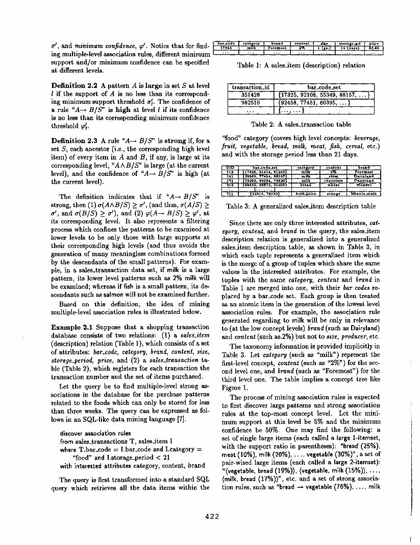
u’, and minimum confidence, cp’. Notice that for find- b?,:i? i Caz!OLry I pbrrn d cc.llteltt he 1 l tor.geqt* p,,ce OTezllO*t a* I 1 (la.) I 14 (days) 1 83.99

ing multiple-level association rules, different minimum . ’ . ’ . . . . . . . . . . . .

support and/or minimum confide&e can be specified at different levels.

Table 1: A salesitem (description) relation

Definition 2.2 A pattern A is large in set S at level 1 if the support of A is no less than its corresponding minimum support threshold CT;. The confidence of a rule “A- B/S’ is high at level I if its confidence is no less than its corresponding minimum confidence threshold (o’, .

Definition 2.3 A rule “A+ B/S” is strong if, for a set S, each ancestor (i.e., the corresponding high level item) of every item in A and B, if any, is large at its corresponding level, “A A B/S” is large (at the current level), and the confidence of “A+ B/S” is high (at the current level).

The definition indicates that if “A+ B/S’ is strong, then (1) u(AAB/S) >_ u’, (and thus, c(A/S) 2 u’, and u(B/S) 2 a’), and (2) cp(A+ B/S) 1 ‘p’, at its corresponding level. It also represents a filtering process which confines the patterns to be examined at lower levels to be only those with large supports at their corresponding high levels (and thus avoids the generation of many meaningless combinations formed by the descendants of the small patterns). For example, in a sales-transaction data set, if milk is a large pattern, its lower level patterns such as 2% milk will be examined; whereas if fish is a small pattern, its descendants such as salmon will not be examined further.

Based on this definition, the idea of mining multiple-level association rules is illustrated below.

Example 2.1 Suppose that a shopping transaction database consists of two relations: (1) a sales-item (description) relation (Table l), which consists of a set of attributes: bar-code, category, brand, content, site, storage-period, price, and (2) a sales-transaction table (Table 2), which registers for each transaction the transaction number and the set of items purchased.

Let the query be to find multiple-level strong associations in the database for the purchase patterns related to the foods which can only be stored for less than three weeks. The query can be expressed as follows in an SQL-like data mining language [7].

discover association rules from sales-transactions T, salesitem I where T.bar-code = I.bar-code and I.category =

“food” and I.storage-period < 21 with interested attributes category, content, brand

The query is first transformed into a standard SQL query which retrieves all the data items within the

transaction-id barrodeset 351428 (17325, 92108, 55349, 88157, . . .} 982510 (92458, 77451, 60395, . . . }

. . . I . . . . . . . 1

Table 2: A sales-transaction table

“food” category (covers high level concepts: beverage, fruit, vegetable, bread, milk, meat, fish, cereal, etc.) and with the storage period less than 21 days.

. . . . . , . . . . 711 ( (33314, ?9131) 1 froit-juice ( oranp 1 Minntemaid

Table 3: A generalized salesitem description table

Since there are only three interested attributes, category, content, and brand in the query, the salesitem description relation is generalized into a generalized salesitem description table, as shown in Table 3, in which each tuple rkpiesents a generalized item which is the merge of a group of tuples which share the same values in the interested attributes. For example, the tuples with the same category, content and brand in Table 1 are merged into one, with their bar codes replaced by a bar-code set. Each group is then treated as an atomic item in the generation of the lowest level association rules. For example, the association rule generated regarding to milk will be only in relevance to (at the low concept leyels) grand (such as Dairyland) and content (such as,2%) but not to size, producer, etc.

The taxonomy information is provided implicitly in Table 3. Let category (such as “milk”) represent the first-level concept, content (such as “2%,,) for the second level one, and brand (such as “Foremost”) for the third level one. The table implies a concept tree like Figure 1.

The process of mining association rules is expected to first discover large: patterns and strong association rules at the top-most concept level. Let the minimum support at this level be 5% and the minimum confidence be 50%. One may find the following: a set of single large items (each called a large 1-itemset, with the support ratio in parentheses): “bread (25%), meat (lo%), milk (20%), . . . , vegetable (30%)“, a set of pair-wised large items (each called a large 2-itemset): “(vegetable, bread (19%)), (vegetable, milk (15%)), . . . , (milk, bread (17%))“) etc. and a set of strong association rules, such as “bread ---) vegetable (76%), . . . , milk

422

Dairyland Foranost Old Mill8 Wonder

Figure 1: A taxonomy for the relevant data items

+ bread (85%)“.

At the second level, only the transactions which contain the large items at the first level are examined. Let the minimum support at this level be 2% and the minimum confidence be 40%. One may find the following large 1-itemsets: “lettuce (10%) wheat bread (15%), white bread (10%) 2% milk (10%) chicken (5%), . . . , beef (5%)“, and the following large 2- itemsets: “(2% milk, wheat bread (6%)), (lettuce, 2% milk (4%)), (chicken, beef (2.1%))“, and the strong association rules: “2% milk --) wheat bread (60%), . . . , beef -+ chicken (42%)“, etc.

The process repeats at even lower concept levels until no large patterns can be found. 0

3 A method for mining multiple-level association rules

A method for mining multiple-level association rules is introduced in this section, which uses a hierarchy- information encoded transaction table, instead of the original transaction table, in iterative data mining. This is based on the following considerations. First, a data mining query is usually in relevance to only a portion of the transaction database, such as food instead of all the items. It is beneficial to first collect the relevant set of data and then work repeatedly on the task-relevant set. Second, encoding can be performed during the collection of task-relevant data, and thus there is no extra “encoding pass” required. Third, an encoded string, which represents a position in a hierarchy, requires less bits than the corresponding object- identifier or bar-code. Moreover, encoding makes more items to be merged (or removed) due to their identical encoding, which further reduces the size of the encoded transaction table. Thus it is often beneficial to use an encoded table although our method does not ,rely on the derivation of such an encoded table because the encoding can always be performed on the fly.

To simplify our discussion, an abstract example which simulates the real life example of Example 2.1 is analyzed as follows.

Example 3.1 As stated above, the taxonomy information for each (grouped) item in Example 2.1 is en-

coded as a sequence of digits in the transaction table 7[1] (Table 4). F or example, the item ‘2% Foremost milk’ is encoded as ‘112’ in which the first digit, ‘l’, represents ‘milk’ at level-l, the second, ‘I’, for ‘2% (milk)’ at level-2, and the third, ‘2’, for the brand ‘Foremost’ at level-3. Similar to [2], repeated items (i.e., items with the same encoding) at any level will be treated as one item in one transaction.

TID 1 Items Tl I {ill, 121, 211, 221)

1 i /!Ezf&4131 Table 4: Encoded transaction table: 7[1]

The derivation of the large item sets at level 1 proceeds as follows. Let the minimum support be 4 transactions (i.e., minsup[l] = 4). (Notice since the total number of transactions is fixed, the support is expressed in an absolute value rather than a relative per- centage for simplicity). The level-l large 1-itemset table ,C[l, l] can be derived by scanning 7[1], registering support of each generalized item, such as l**, . . . ,4**, if a transaction contains such an item (i.e., the item in the transaction belongs to the generalized item l**, . ..) 4**, respectively), and filtering out those whose accumulated support count is lower than the minimum support. C[l, l] is then used to filter out (1) any item which is not large in a transaction, and (2) the transactions in 7[1] which contain only small items. This results in a filtered transaction table 7[2] of Figure 2. Moreover, since there are only two entries in f[l,l], the level-l large-2 itemset table L[1,2] may contain only 1 candidate item {l**, 2**}, which is supported by 4 transactions in 7[2].

Level-l minsup = 4 Level-l large 1-itemsets: Filtered transaction table:

Figure 2: Large item sets at level 1 and filtered transaction table: 7[2]

According to the definition of ML-association rules,

423

Level-2 minsup = 3 Level-2 large 1-itemsets: Level-2 large 3-itemsets:

( {;::i 1 t ( Level-3 minsup = 3 Level-3 large 1-itemsets:

fY3.11

Level-2 large P-itemsets: L12.21

Itemset Itemset support support {ll*, 12*} {ll*, 12*} 4 4 {ll*, 21*) {ll*, 21*) 3 El 3 I {ll*, 22*} 1 {ll*, 22*} 4 4 {12*, 22*} {12*, 22*} 3 3 {21*, 22*} {21*, 22*} 3 3

-L-l-, Itemset Support (111) 4

1 (211) 4 (221) 3

Level-3 large 2-itemsets: -L[3,2l

-1

Figure 3: Large item sets at levels 2 and 3

only the descendants of the large items at level-l (i.e., in C[l ,l]) are considered as candidates in the level-2 large 1-itemsets. Let minsup[2] = 3. The level-2 large 1-itemsets L[2,1] can be derived from the filtered transaction table 7[2] by accumulating the support count and removing those whose support is smaller than the minimum support, which results in C[2,1] of Figure 3. Similarly, the large a-item& table t[2,2] is formed by the combinations of the entries in t[2,1], together with the support derived from 7[2], filtered using the corresponding threshold. The large 3-itemset table L[2,3] is formed by the combinations of the entries in C[2,2] (which has only one possibility {ll*, 12*, 22*)), and a similar process.

Finally, C[3,1] and C[3,2] at level 3 are computed in a similar process, with the results shown in Figure 3. The computation terminates since there is no deeper level requested in the query. Note that the derivation also terminates when an empty large 1-itemset table is generated at any level. cl

The above discussion leads to the following algorithm for mining strong ML-association rules.

Algorithm 3.1 (ML-T2Ll) Find multiple-level large item sets for mining strong ML association rules in a transaction database.

Input: (1) 7[1], h a ierarchy-information-encoded and task-relevant set of transaction database, in the format of (TID, Itemset), in which each item in the Itemset contains encoded concept hierarchy information, and (2) the minimum support threshold (minsup[Q for each concept level 1.

Output: Multiple-level large item sets.

Method: A top-down, progressively deepening process which collects large item sets at different concept levels as follows.

Starting at level 1, derive for each level 1, the large h-items sets, L[I, E], for each k, and the large item set, U[l] (for all k’s), as follows (in the syntax similar to C and Pascal, which should be self-explanatory).

(1) for (I := 1; L[l, 1] # fl and 1 < max-level; I++) do {

[ii if I= 1 then {

q, 11 := get-large-litemsels(T[l], I);

(4 T[2] := ge2-fiZteredffabZe(l[l], L[l, 11); (5) 1

g else &[I, 1] := getJargeAAemsets(7[2], Q; for (k := 2; L[l, k - 1] # 0; k++) do {

ck := get-candidateset(&[~, k - 11); foreach transaction t E 7[2] do (

(10) ct := getmd&?ts(ck, t); (11) foreach candidate c E Ct do c.support++; (12) I

(13) L[l, k] := {c E Cklc.support 2 minsup[q} (14) 1 (15) LL[l] := (J, L[l, k];

(16) 1 q

Explanation of Algorithm 3.1.

According to Algorithm 3.1, the discovery of large support items at each level 1 proceeds as follows.

1. At level 1, the large 1-itemsets C[l, l] is derived from 7[1] by “get-large-15!emsets(l[l], 1)“. At any other level 1, Z[l, l] is derived from 7[2] by “gethrge_l,itemsets(7[2], I)“, and notice that when 1 > 2, only the item in L[l - 1, l] will be considered when examining 7[2] in the derivation of the large 1-itemsets t[l, 11. This is implemented by scanning the items of each transaction t in 7[1] (or 7[2]), incrementing the support count of an item i in the itemset if i’s count has not been incremented by t. After scanning the transaction table, filter out those items whose support is smaller than minsup[lj.

The filtered transaction table 7[2] is derived by “get-filtered-t-ta,ble(l[l], C[l, 11)“) which uses L[l,l] as a filter to filter out (1) any item which is not large at level 1, and (2) the transactions which contain no large items.

The large k (for k > 1) item set table at level 1 is derived in two steps:

(a) Compute the candidate set from L[l, k-l], as done in the apriori candidate generation algorithm [2], apriori-gen, i.e., it first generates a set Ck in which each item set consists of k items, derived by joining two (k - 1) items

424

in L[I, h] which share (k - 2) items, and then removes a k-itemset c from Ck if there exists a c’s (, - 1) subset which is not in C[/, B - 11.

(b) For each transaction t in 7[2], for each of t’s k-item subset c, increment c’s support count if c is in the candidate set Ck. Then collect into L[I, E] each c (together with its support) if its support is no less than minsup[lj.

4. The large itemsets at level I, fX[Zj, is the union of L[I, Ic] for all the k’s 0

After finding the large itemsets, the set of association rules for each level I can be derived from the large itemsets CL[/j baaed on the minimum confidence at this level, minconf[lj. This is performed as follows [2]. For every large itemset r, if a is a nonempty subset of r, the rule “a-+ r - u” is inserted into rule-set[lj if support(r)/support(a) > minconf[ll, where minconf[q is the minimum confidence at level 1.

Algorithm ML-T2Ll inherits several important optimization techniques developed in previous studies at finding association rules [l, 21. For example, get-candidate-set of the large k-itemsets from the known large (k - 1)-itemsets follows apriori-gen of Al- gorithm Apriori [2]. Function get-SUbSetS(Ck , t) is implemented by a hashing technique from [2]. Moreover, to accomplish the new task of mining multiple-level association rules, some interesting optimization techniques have been developed, as illustrated below.

1. Generalization is first performed on a given item description relation to derive a generalized item table in which each tuple contains a set of item identifiers (such as bar-codes) and is encoded with concept hierarchy information.

2. The transaction table 7 is transformed into 7[1] with each item in the itemset replaced by its corresponding encoded hierarchy information.

3. A filtered transaction 7[2] which filters out small items at the top level of 7[1] using the large l- itemsets L[l,l] d is erived and used in the derivation of large L-items for any L (k: > 1) at level-l and for any k (h 2 1) for level I (I > 1).

4. From level 1 to level (I + l), only large items at C[1, l] are checked against 7[2] for L[I + 1, 11.

Notice that in the processing, 7[1] needs to be scanned twice, whereas 7[2] needs to be scanned p times where p = C, Lr - 1, and )I is the maximum k such that the k-itemset table is nonempty at level I.

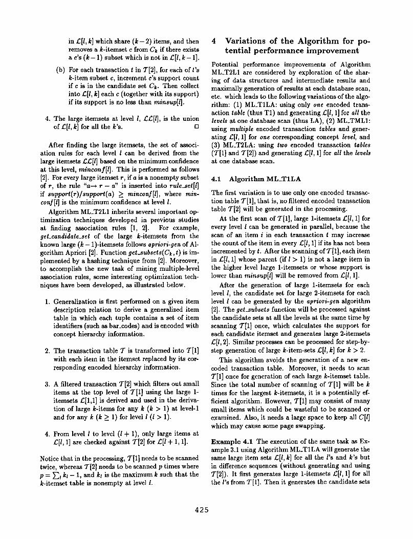
4 Variations of the Algorithm for potential performance improvement

Potential performance improvements of Algorithm ML-T2Ll are considered by exploration of the sharing of data structures and intermediate results and maximally generation of results at each database scan, etc. which leads to the following variations of the algorithm: (1) ML-TlLA: using only one encoded transaction table (thus Tl) and generating C[I, l] for all the levels at one database scan (thus LA), (2) ML-TMLl: using multiple encoded transaction tables and generating L[I, l] for one corresponding concept level, and (3) ML-TSLA: using two encoded transaction tables (7[1] and 7[2]) and g enerating C[I, l] for all the levels at one database scan.

4.1 Algorithm ML-TlLA

The first variation is to use only one encoded transaction table 7[1], that is, no filtered encoded transaction table 7[2] will be generated in the processing.

At the first scan of 7[1], large 1-itemsets ,C[i, l] for every level 1 can be generated in parallel, because the scan of an item i in each transaction t may increase the count of the item in every ,!Z[l, l] if its has not been incremented by t . After the scanning of I[ 11, each item in .C[1, l] whose parent (if I > 1) is not a large item in the higher level large 1-itemsets or whose support is lower than minsup[l] will be removed from c[l, 11.

After the generation of large 1-itemsets for each level 1, the candidate set for large 2-itemsets for each level 1 can be generated by the apriori-gen algorithm [2]. The get-subsets function will be processed against the candidate sets at all the levels at the same time by scanning 7[1] once, which calculates the support for each candidate itemset and generates large 2-itemsets L[I, 21. Similar processes can be processed for step-by- step generation of large h-item-sets L[I, k] for k > 2.

This algorithm avoids the generation of a new encoded transaction table. Moreover, it needs to scan 7[1] once for generation of each large h-itemset table. Since the total number of scanning of 7[1] will be JZ times for the largest lc-itemsets, it is a potentially efficient algorithm. However, 7[1] may consist of many small items which could be wasteful to be scanned or examined. Also, it needs a large space to keep all C[Zj which may cause some page swapping.

Example 4.1 The execution of the same task as Ex- ample 3.1 using Algorithm ML-TlLA will generate the same large item sets L[I, k] for all the l’s and k’s but in difference sequences (without generating and using 7[2]). It first generates large 1-itemsets t[l, l] for all the l’s from 7[1]. Then it generates the candidate sets

425

from L[Z, 11, and then derives large P-itemsets ,C[I, 21 by passing the candidate sets through 7[1] to obtain the support count and filter those smaller than minsup[l]. This process repeats to find k-itemsets for larger k until all the large k-item&s have been derived. 0

4.2 Algorithm ML-TMLl

The second variation is to generate multiple encoded transaction tables 7[1], 7[2], . . . ,7[[maz_l+l], where max_l is the maximal level number to be examined in the processing.

Similar to Algorithm ML-TPLl, the first scan of 7[1] generates the large 1-itemsets L[l, l] which then serves as a filter to filter out from 7[1] any small items or transactions containing only small items. 7[2] is resulted from this filtering process and is used in the generation of large k-itemsets at level 1.

Different from Algorithm ML-TPLl, 7[2] is not repeatedly used in the processing of the lower levels. In- stead, a new table 7[1+ l] is generated at the processing of each level I, for 1 > 1. This is done by scanning 7[Zj to generate the large 1-itemsets t[l, l] which serves as a filter to filter out from 7[fl any small items or transactions containing only small items and results in 7[1+1] which will be used for the generation of large k-itemsets (for k > 1) at level 1 and table T[I + 21 at the next lower level. Notice that as an optimization, for each level 1 > 1, 7[/j and L[I, l] can be generated in parallel (i.e., at the same scan).

The algorithm derives a new filtered transaction table, 7[1+ 11, at the processing of each level 1. This, though seems costly at generating several transaction tables, may save a substantial amount of processing if only a small portion of data are large items at each level. Thus it may be a promising algorithm in this circumstance. However, it may not be so effective if only a small number of the items will be filtered out at the processing of each level.

Example 4.2 The execution of the same task as Ex- ample 3.1 using Algorithm ML-TMLl will generate the same large itemsets f[I, k] for all the I’s and k’s but in difference sequences, with the generation and help of the filtered transaction tables 7[2], . . . , I[maxJ + 11, where maxi is the maximum level explored in the algorithm. It first generates the large 1-itemsets L[l, l] for level 1. Then for each level 1 (initially 1 = l), it generates the filtered transaction table 7[I + l] and the level-(Z + 1) large 1-itemsets L[Z + 1, l] by scanning 7[/l using C[I, 11, and then generates the candidate 2-itemsets from t[l, 11, calculates the supports using 7[l+ 11, filters those with support less than minsup[q, and derives c[Z, 21. The process repeats for the derivation of L[Z, 31, . . . , L[Z, k]. 0

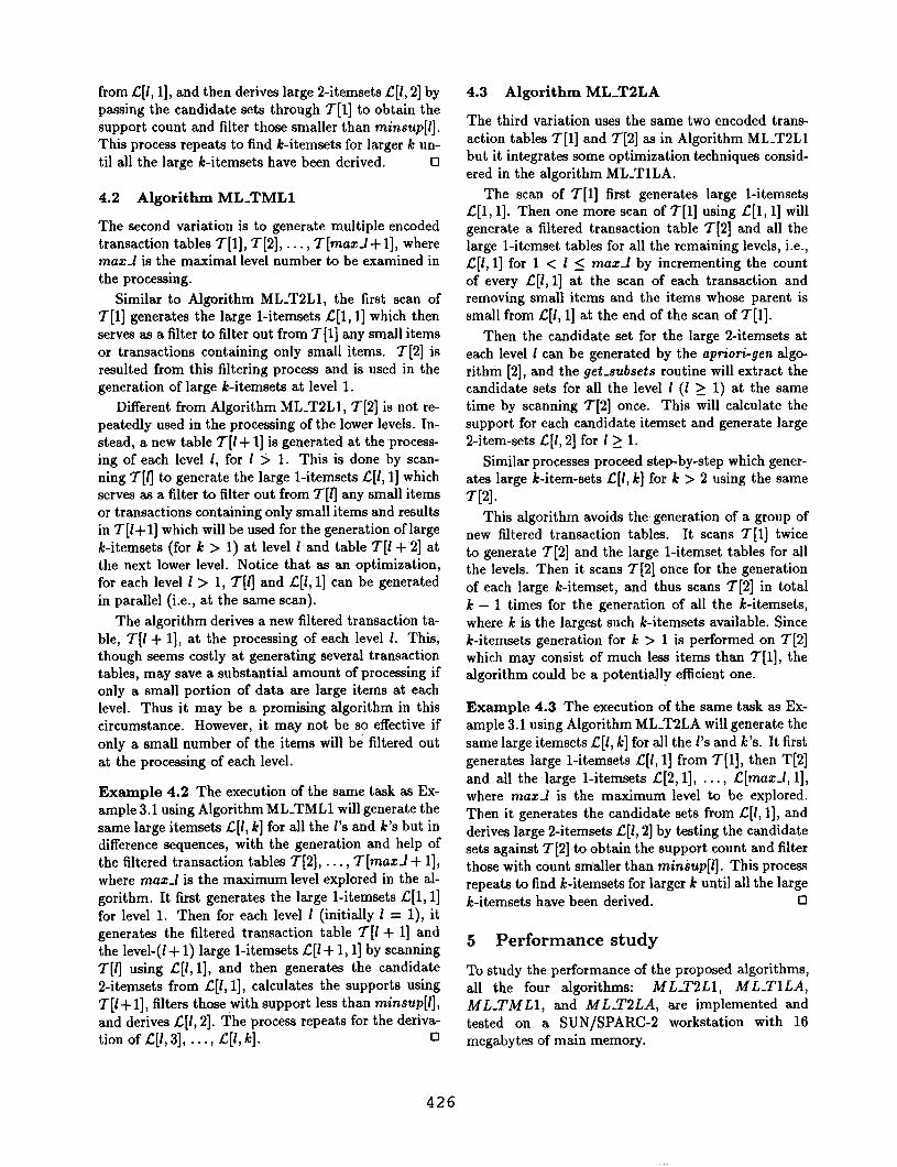
4.3 Algorithm ML-T2LA

The third variation uses the same two encoded transaction tables 7[1] and 7[2] as in Algorithm ML-T2Ll but it integrates some optimization techniques considered in the algorithm ML-TlLA.

The scan of 7[1] first generates large 1-itemsets L[l, 11. Then one more scan of 7[1] using L[l, l] will generate a filtered transaction table 7[2] and all the large 1-itemset tables for all the remaining levels, i.e., C[Z, l] for l- < I 5 maxi by incrementing the count of every ,C[l, l] at the scan of each transaction and removing small items and the items whose parent is small from L[Z, l] at the end of the scan of 7[1].

Then the candidate set for the large 2-itemsets at each level 1 can be generated by the aption’-gen algorithm [2], and the get-subsets routine will extract the candidate sets for all the level 1 (I 1 1) at the same time by scanning 7[2] once. This will calculate the support for each candidate itemset and generate large a-item-sets Lc[I, 21 for 1 3 1.

Similar processes proceed step-by-step which generates large k-item-sets t[l, k] for k > 2 using the same

WI- This algorithm avoids the, generation of a group of

new filtered transaction tables. It scans 7111 twice to generate 7[2] and the large 1-itemset tables for all the levels. Then it scans 7[2] once for the generation of each large k-itemset, and thus scans 7[2] in total k - 1 times for the generation of all the k-itemsets, where k is the largest such k-itemsets available. Since k-itemsets generation for k > 1 is performed on 7[2] which may consist of much less items than 7[1], the algorithm could be a potentially efficient one.

Example 4.3 The execution of the same task as Ex- ample 3.1 using Algorithm ML-TSLA will generate the same large itemsets ,C[1, k] for all the Z’s and k’s. It first generates large 1-itemsets L[I, l] from 7[1], then T[2] and all the large 1-itemsets C[2,1], . . . , ~[max-l, 11, where maz-l is the maximum level to be explored. Then it generates the candidate sets from L[1,1], and derives large P-itemsets Lc[I, 21 by testing the candidate sets against 7[2] to obtain the support count and filter those with count smaller than minsup[q. This process repeats to find k-itemsets for larger k until all the large k-itemsets have been derived. 0

5 Performance study

To study the performance of the proposed algorithms, all the four algorithms: ML-7’2~51, MLTlLA, ML-TMLl, and ML-TBLA, are implemented and tested on a SUN/SPARC-2 workstation with 16 megabytes of main memory.

426

The testbed consists of a set of synthetic transaction databases generated using a randomized item set generation algorithm similar to that described in [2].

The following are the basic parameters of the generated synthetic transaction databases: (1) the total number of items, I, is 1000; (2) the total number of transactions is 100,000; and (3) 2000 potentially large itemsets are generated and put into the transactions based on some distribution. Table 5 shows the database used, in which S is the average size (# of items in a potential large itemset) of these itemsets, and T is the average size (# of items in a transaction) of a transaction.

Database S T # of transactions Size(MBytes) DBl 2 5 100,000 2.7MB DB2 4 10 100.000 4.7MB

Table 5: Transaction databases

Each transaction, database is converted into an encoded transaction table, denoted as 7[1], according to the information about the generalized items in the item description (hierarchy) table. The maximal level of the concept hierarchy in the item table is set to 4. The number of the top level nodes keeps increas- ing until the total number of items reaches 1000. The fan-outs at the lower levels are selected based on the normal distribution with mean value being M2, M3, and M4 for the levels 2, 3, and 4 respectively, and a variance of 2.0. These parameters are summarized in Table 6.

Item Table #nodes at level-l M2 M3 M4 Zl 8 5 5 5

12 15 6 3 4

Table 6: Parameters settings of the item description (hierarchy) tables

The testing results presented in this section are on two synthetic transaction databases: one, TlO (DB2), has an average transaction size (# of item in a transaction) of 10; while the other, T5 (DBl), has an average transaction size of 5.

Two item tables are used in the testing: the first one, 11, has 8, 5, 5 and 5 branches at the levels 1, 2, 3, and 4 respectively; whereas the second, 12, has 15, 6, 3 and 4 branches at the corresponding levels.

Figure 4 shows the running time of the four algorithms in relevance to the number of transactions in the database. The test uses the database TlO and the item set 11, with the minimum support thresholds being (50,10,4,2), which indicates that the minimum support of level 1 is 50%, and that of levels 2,3 and 4 are respectively lo%, 4%, and 2%.

The four curves in Figure 4 show that MLTPLA has the best performance, while the ML-TlLA has the worst among the four algorithms under the current threshold setting. This can be explained as follows. Since the first threshold filters out many small 1-itemsets at level 1 which results in a much smaller filtered transaction table 7[2], but the later filter is not so strong and parallel derivation of C[I, 61 without derivation of 7[3] and 7[4] is more beneficial, thus leads ML-T2LA to be the best algorithm. On the other hand, ML-TlLA is the worst since it consults a large 7111 at every level.

UT10

24 4

20 'TlLA' -+- 'T2Ll' -E--

25k 5Ok 75k IOOk #ofVansactbns

Figure 4: Threshold (50, 10, 4, 2)

Figure 5 shows that ML-TlLA is the best whereas ML-TMLl the worst among the four algorithms under the setting: a different test database T5, the same item set II, and with the minimum support thresholds: (20,8,2,1). This is because the first threshold filters out few small 1-itemsets at level 1 which results in almost the same sized transaction table 7[2]. The generation of multiple filtered transaction tables is largely wasted, which leads the worst performance of ML_TMLl. Thus parallel derivation of C[I, k] without derivation of any filtered transaction tables applied in ML,TlLA leads to the best performance.

Figure 6 shows that MLYSLl and ML-TMLl are closely the best whereas M L-TSLA and ML-TlLA the worst under the setting: a test database TlO, an item set 12, and with the minimumsupport thresholds: (50,10,5,2). Th is is because the first threshold filters out relatively more 1-itemsets at level 1 which results in small transaction table 7[2]. Thus the generation of multiple filtered transaction tables is relatively beneficial. Meanwhile, the generation of multiple level large 1-itemsets may not save much because one may still obtain reasonably good sized itemsets in the current setting, which leads ML-T2Ll to be the best perfor-

427

HT5

25

20 ‘TlLA’ + ‘T2Ll’ -e-

15

I 1 I I 25k 5ok 75k 1OOk

# ot transactbns

Figure 5: Threshold (20, 8, 2, 1) Figure 7: Threshold (30, 15, 5, 2)

mance algorithm.

25

‘T2LA’ -x-- 20 ‘TMLl’ +

15

25k 50k 75k 1OOk # ot transactbns

Figure 6: Threshold (50, 10, 5, 2)

Figure 7 shows that ML-TMLl is the best whereas MLYlLA the worst under the setting: a test database T5, an item set 12, and with the minimum support thresholds: (30,15,5,2). This is because every threshold filters out relatively many 1-itemsets at each level which results in much smaller transaction tables at each level. Thus the generation of multiple filtered transaction tables is beneficial, which leads to ML_TMLl is the best, and then ML_TBLl, ML-TSLA and ML_TlLA in sequence.

The above four figures show two interesting fea- tures. First, the relative performance of the four algo rithms under any setting is relatively independent of the number of transactions used in the testing, which indicates that the performance is highly relevant to the threshold setting (i.e., the power of a filter at each

0

‘TllA’ + ‘T2Ll’ -a--

6

“1Ok 25k # ot tn%htbns

75k 1OOk

level). Thus based on the effectiveness of a threshold, a good algorithm can be selected to achieve good performance. Second, all the algorithms have relatively good “scale-up” behavior since the increase of the number of transactions in the database will lead to approximately the linear growth of the processing time, which is desirable in the processing of large transaction databases.

Figure 8 shows the running time of the four algorithms in relevance to the minimum support thresholds. The test uses the database TlO and the item set 12, with a sequence of threshold settings: threl, . . . , thre6. The setting of thwl is (60,15,5,2) (with the same notational convention). The remaining threshold settings are as follows: threB: (55,15,5,2), thre9: (55,10,5,2), thre4: (50,10,5,2), thred: (50,10,5, l), threk (50,5,2,1). The value-decreasing sequence of minimum support thresholds indicates that weaker filtering mechanism is applied to the later portion of the sequence.

The relative performance of the four algorithms shows the interesting trends of growth as indicated by the four curves in Figure 8. The stronger the filtering mechanism, the more 1-itemsets are filtered out at each level, and the smaller large 1-itemsets are resulted in. Thus MLYMLl, which generates a sequence of filtered transaction tables, has the lowest cost at threl, thre% and also (but marginally) threJ, but the highest cost at thre5 and thre6 (since few items are filtered out). On the contrary, ML-TlLA, which uses only one encoded transaction table but generates the large 1-itemsets for each level at the beginning has the highest cost at threl, thrd? and thre.9, but the lowest cost at threb. The other two algorithms stand in, the middle with MLY2LA performs the best at threb when the threshold is reasonable small, especially at the lower levels, and ML-T2Ll performs the best at thre4 when

428

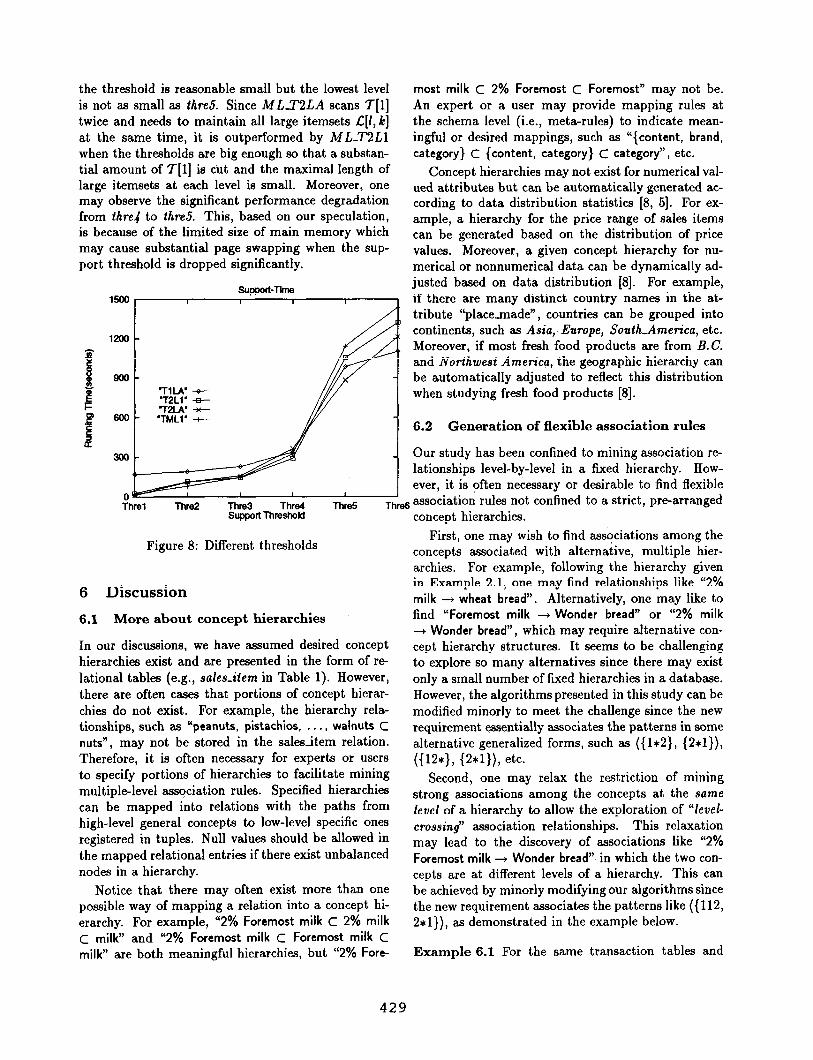
the threshold is reasonable small but the lowest level is not as small as the5 Since ML-T2LA scans 7[1] twice and needs to maintain all large itemsets L[I,)] at the same time, it is outperformed by ML_TSLl when the thresholds are big enough so that a substantial amount of 7[1] is cut and the maximal length of large itemsets at each level is small. Moreover, one may observe the significant performance degradation from thre.# to &e5. This, based on our speculation, is because of the limited size of main memory which may cause substantial page swapping when the support threshold is dropped significantly.

1500

1200

FL

P

i 600

z

300

most milk c 2% Foremost c Foremost” may not be. An expert or a user may provide mapping rules at the schema level (i.e., meta-rules) to indicate meaningful or desired mappings, such as “{content, brand, category} C {content, category} C category”, etc.

Concept hierarchies may not exist for numerical val- ued attributes but can be automatically generated according to data distribution statistics [8, 51. For example, a hierarchy for the price range of sales items can be generated based on the distribution of price values. Moreover, a given concept hierarchy for numerical or nonnumerical data can be dynamically adjusted based on data distribution [S]. For example, if there are many distinct country names in the attribute “placemade”, countries can be grouped into continents, such as Asia, Europe, South-America, etc. Moreover, if most fresh food products are from B.C. and Northwest Americg, the geographic hierarchy can be automatically adjusted to reflect this distribution when studying fresh food products [S].

6.2 Generation of flexible association rules

Our study has been confined to mining association relationships level-by-level in a fixed hierarchy. How- ever, it is often necessary or desirable to find flexible

FE fhrel Thre2 ThfB3 Thre4 Thre5 Ttrd association rules not confined to a strict, pm-arranged

supp0rtmtw0kl concept hierarchies.

Figure 8: Different thresholds

6 Discussion

6.1 More about concept hierarchies

In our discussions, we have assumed desired concept hierarchies exist and are presented in the form of relational tables (e.g., sales-item in Table 1). However, there are often cases that portions of concept hierarchies do not exist. For example, the hierarchy relationships, such as “peanuts, pistachios, . . . , walnuts C nuts”, may not be stored in the sales-item relation. Therefore, it is often necessary for experts or users to specify portions of hierarchies to facilitate mining multiple-level association rules. Specified hierarchies can be mapped into relations with the paths from high-level general concepts to low-level specific ones registered in tuples. Null values should be allowed in the mapped relational entries if there exist unbalanced nodes in a hierarchy.

Notice that there may often exist more than one possible way of mapping a relation into a concept hierarchy. For example, “2% Foremost milk C 2% milk c milk” and “2% Foremost milk C Foremost milk C milk” are both meaningful hierarchies, but “2% Fore-

First, one may wish to find associations among the concepts associated with alternative, multiple hierarchies. For example, following the hierarchy given in Example 2.1, one may find relationships like “2% milk -+ wheat bread”. Alternatively, one may like to find “Foremost milk --* Wonder bread” or “2% milk + Wonder bread”, which may require alternative concept hierarchy structures. It seems to be challenging to explore so many alternatives since there may exist only a small number of fixed hierarchies in a database. However, the algorithms presented in this study can be modified minorly to meet the challenge since the new requirement essentially associates the patterns in some alternative generalized forms, such as ({1*2}, {2*1}), ({12*), {2*1}), etc.

Second, one may relax the restriction of mining strong associations among the concepts at the same level of a hierarchy to allow the exploration of “level- crossing” association relationships. This relaxation may lead to the discovery of associations like “2% Foremost milk + Wonder bread” in which the two concepts are at different levels of a hierarchy. This can be achieved by minorly modifying our algorithms since the new requirement associates the patterns like ({ 112, 2*1}), as demonstrated in the example below.

Example 6.1 For the same transaction tables and

429

concept hierarchies given in Example 3.1, we examine the mining of strong multiple-level association rules which includes nodes at different levels in a hierarchy.

Let minimum support at each level be: minsup = 4 at level-l, and minsup = 3 at levels 2 and 3.

The derivation of the large itemsets at level 1 proceeds in the same way as in Example 3.1, which generates the same large itemsets tables Ic[l, l] and ,C[1,2] at level 1 and the same filtered transaction table 7[2], as shown in Figure 2.

The derivation of level-2 large itemsets generates the same large 1-itemsets fJ2, l] as shown in Figure 9. However, the candidate items are not confined to pair- ing only those in t[2, l] because the items in t[2, l] can be paired with those in C[l, l] as well, such as { ll*, 1~) (for potential associations like “milk - 2% milk”), or {ll*, 2~) (for potential associations like “2% milk -+ bread”). These candidate large 2-itemsets will be checked against 7[2] to find large items (for the level-mixed nodes, the minimum support at a lower level, i.e., minsup[2], can be used as a default). Such a process generates the large 2-itemsets table t[2,2] as shown in Figure 9.

Notice that the table does not include the a-item pairs formed by an item with its own ancestor such as ({ ll*, l**}, 5) since its support must be the same as its corresponding large 1-itemset in C[2,i], i.e., ({ll*}, 5), based on the set containment relationship: any transaction that contains {ll*) must contain (1~) as well.

Similarly, the level 2 large 3-itemsets C[2,3] can be computed, with the results shown in Figure 9. Also, the entries which pair with their own ancestors are not listed here since it is contained implicitly in their corresponding P-item&s. For example, ({ll*, 12*}, 4) in C[2,2] implies ({ll*, 12*, l**}, 4) in L[2,3].

Level-Z minsup = 3 Level-Z large l-item&:

~[~11 Itemset Support {ll*} 5

m

{12*} 4

Ii:*1 4 * 4

Level-2 large 2-itemset: - 21

T w,

Itemset I= {ll*, 12*} {ll*, 21*}

Level-2 large 3-itemset:

*, / i;z;;;i

support 4 3 4 3

1 3 4 3 3 4

Figure 9: Large Item Sets at Level 2

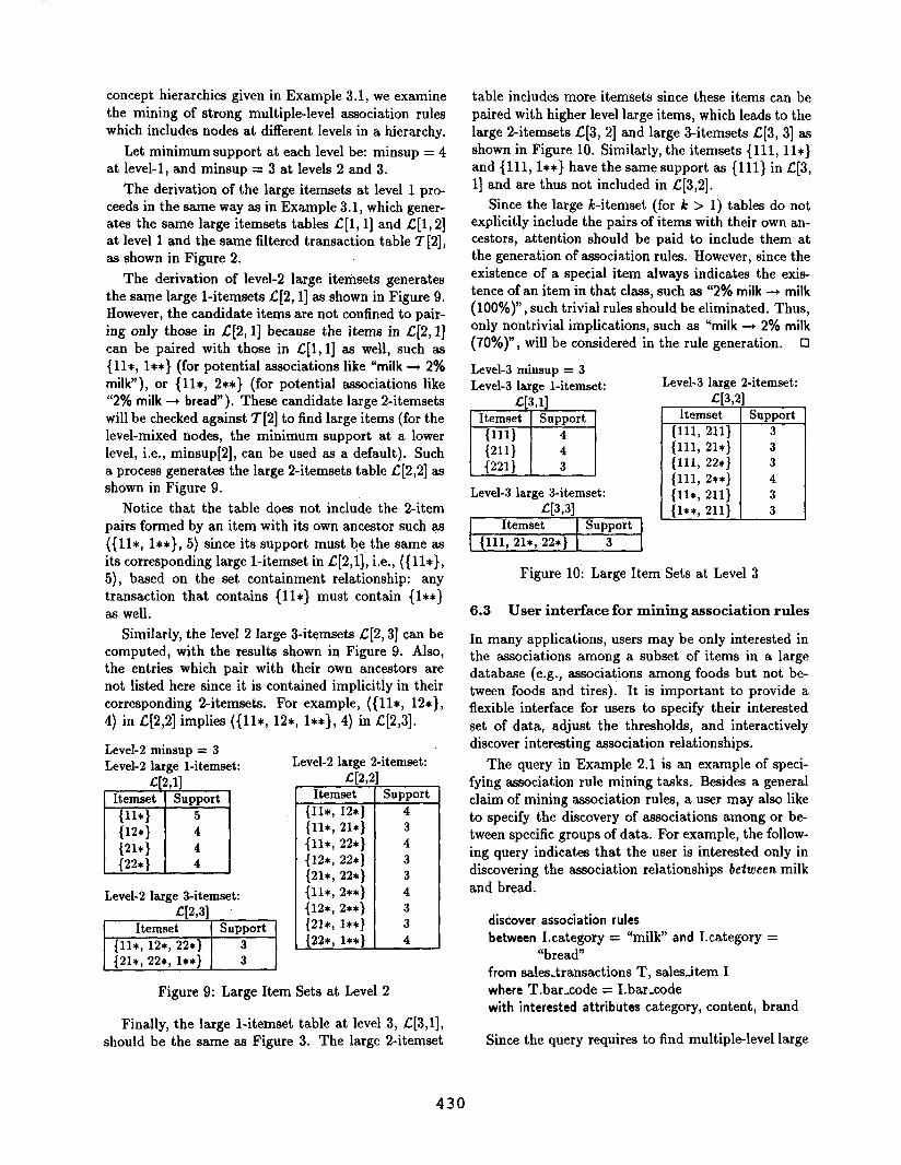
Finally, the large 1-itemset table at level 3, C[3,1], should be the same as Figure 3. The large 2-itemset

table includes more itemsets since these items can be paired with higher level large items, which leads to the large 2-itemsets C[3, 21 and large 3-itemsets t[3, 31 as shown in Figure 10. Similarly, the itemsets { 111, 1 l*} and (111, 1~) have the samesupport as (111) in ~5[3, l] and are thus not included in t[3,2].

Since the large L-itemset (for Jz > 1) tables do not explicitly include the pairs of items with their own ancestors, attention should be paid to include them at the generation of association rules. However, since the existence of a special item always indicates the exis tence of an item in that class, such as “2% milk -+ milk (loo%)“, such trivial rules should be eliminated. Thus, only nontrivial implications, such as “milk + 2% milk (70%)“) will be considered in the rule generation. 0

Level-3 minsup = 3 Level-3 lame 1-itemset: Level-3 large 2-itemset:

q3:11 c[3,21 Itemset Support Itemset Support

I (111) 4 (111, 211) 3

Ii::; 4

(111, 21*} 3

3 (111, 22*} 3 (111, 2**} 4

Level-3 large I-itemset: L[3,31 _-i-

{ll*, 211) 3

-1 {l**, 2111 3

Figure 10: Large Item Sets at Level 3

1

6.3 User interface for mining association rules

In many applications, users may be only interested in the associations among a subset of items in a large database (e.g., associations among foods but not between foods and tires). It is important to provide a flexible interface for users to specify their interested set of data, adjust the thresholds, and interactively discover interesting association relationships.

The query in Example 2.1 is an example of speci- fying association rule mining tasks. Besides a general claim of mining association rules, a user may also like to specify the discovery of associations among or between specific groups of data. For example, the following query indicates that the user is interested only in discovering the association relationships betureen milk and bread.

discover association rules between I.category = “milk” and Icategory =

“bread” from sales-transactions T, salesitem I where T.bar-code = I.bar-code with interested attributes category, content, brand

Since the query requires to find multiple-level large

430

2-itemsets only, the rule mining algorithm needs to be modified accordingly, however, it will preserve the same spirit of sharing structures and computations among multiple levels.

Graphical user interface is recommended for dynamic specification and adjustment of a mining task and for level-by-level, interactive, and progressive mining of interesting relationships. Moreover, graphical outputs, such as graphical representation of discovered rules with the corresponding levels of the concept hierarchies may substantially enhance the clarity of the presentation of multiple-level association rules.

7 Conclusions

We have extended the scope of the study of mining association rules from single level to multiple concept levels and studied methods for mining multiple-level association rules from large transaction databases. A top-down progressive deepening technique is developed for mining multiple-level association rules, which extends the existing single-level association rule mining algorithms and explores techniques for sharing data structures and intermediate results across levels. Based on different sharing techniques, a group of algorithms, notably, ML-TSLl, ML-TlLA, ML-TMLl and ML-TPLA, have been developed. Our performance study shows that different algorithms may have the best performance for different distributions of data.

Related issues, including concept hierarchy han- dling, methods for mining flexible multiple-level association rules, and adaptation to difference mining requests are also discussed in the paper. Our study shows that mining multiple-level association rules from databases has wide applications, and efficient algorithms can be developed for discovery of interesting and strong such rules in large databases.

Extension of methods for mining single-level knowledge rules to multiple-level ones poses many new issues for further investigation. For example, with the recent developments on mining single-level sequential patterns [3] and metaquery guided data mining [16], mining multiple-level sequential patterns and metaquery guided mining of multiple-level association rules are two interesting topics for future study.

References

[l] R. AgrawaI, T. Imielinski, and A. Swami. Mining association rules between sets of items in large databases. In Proc. 1993 ACM-SIGMOD Int. Conf. Management of Data, pp. 207-216, Washington, D.C., May 1993.

[2] R. AgrawaI and R. Srikant. Fast algorithms for mining association rules. In Proc. 1994 Int. Conf. Very Large Data Bases, pp. 487-499, Santiago, Chile, Sept. 1994.

PI

PI

[51

PI

P31

PI

PO1

Pll

WI

P31

P41

P51

[161

R. AgrawaI and R. Srikant. Mining sequential patterns. In Proc. 1995 Int. Conf. Data Engineering, Taipei, Taiwan, March 1995.

A. Borgida and R. J. Brachman. Loading data into description reasoners. In Proc. 1993 ACM-SIGMOD Int. Conf. Management of Data, pp. 217-226, Wash- ington, D.C., May 1993.

W. W. Chu and K. Chiang. Abstraction of high level concepts from numerical values in databases. In AAAI’94 Workshop on Knowledge Discovery in Databases, pp. 133-144, Seattle, WA, July 1994.

D. Fisher. Improving inference through conceptual clustering. In Proc. 1987 AAAI Conf., pp. 461-465, Seattle, Washington, July 1987.

J. Han, Y. Cai, and N. Cercone. Data-driven discovery of quantitative rules in relational databases. IEEE Tmns. Knowledge and Data Engineering, 5:29- 40, 1993.

J. Han and Y. Fu. Dynamic generation and refine- ment of concept hierarchies for knowledge discovery in databases. In AAAI’94 Workshop on Knowledge Dis- covery in Databases, pp. 157-168, Seattle, WA, July 1994.

M. Klemettinen, H. ManniIa, P. Ronkainen, H. Toivo- nen, and A. I. Verkamo. Finding interesting rules from large sets of discovered association rules. In Proc. Srd Int’l Conf. on Information and Knowledge Man- agement, pp. 401-408, Gaithersburg, Maryland, Nov. 1994.

H. ManniIa and K-J. Raiha. Dependency inference. In Proc. 1987 Int. Conf. Very Large Data Bases, pp. 155-158, Brighton, England, Sept. 1987.

R. S. MichaIski and G. Tecuci. Machine Learning, A Multistrategy Approach, Vol. 4. Morgan Kaufmann, 1994.

J.S. Park, M.S. Chen, and P.S. Yu. An effective hash- based algorithm for mining association rules. In Proc. 1995 ACM-SIGMOD Int. Conf. Management of Data, San Jose, CA, May 1995.

G. Piatesky-Shapiro and C. J. Matheus. The interestingness of deviations. In AAAI’94 Workshop on Knowledge Discovery in Databases, pp. 25-36, Seat- tle, WA, July 1994.

G. Piatetsky-Shapiro. Discovery, analysis, and presentation of strong rules. In G. Piatetsky-Shapiro and W. J. Frawley, editors, Knowledge Discovery in Databases, pp. 229-238. AAAI/MIT Press, 1991.

J. R. Quinlan. C4.5: Progmms for Machine Learning. Morgan Kaufmann, 1992.

W. Shen, K. Ong, B. Mitbander, and C. Zaniolo. Metaqueries for data mining. In U.M. Fayyad, G. Piatetsky-Shapiro, P. Smyth, and R. Uthurusamy, editors, Advances in Knowledge Discovery and Data Mining. AAAI/MIT Press, 1995.

431

Discovery of Multiple-Level Association Rules from Large ...

Documents

Transcript of Discovery of Multiple-Level Association Rules from Large ...