rapid modeling and discovery of priority dispatching rules

Journal of Scheduling 9: 7–34, 2006.© 2006 Springer Science + Business Media, Inc. Manufactured in The United States

RAPID MODELING AND DISCOVERY OF PRIORITYDISPATCHING RULES: AN AUTONOMOUS LEARNING

APPROACH

CHRISTOPHER D. GEIGER1, REHA UZSOY2 AND HALDUN AYTUG3

1Department of Industrial Engineering and Management Systems, University of Central Florida, 4000 Central Florida Blvd,Orlando, FL 32816, USA

2Laboratory for Extended Enterprises at Purdue, School of Industrial Engineering, 1287 Grissom Hall, Purdue University,West Lafayette, IN 47907, USA

3Department of Decision and Information Sciences, Warrington College of Business, University of Florida, P.O. Box 117169,Gainesville, FL 32611, USA

ABSTRACT

Priority-dispatching rules have been studied for many decades, and they form the backbone of much industrial schedulingpractice. Developing new dispatching rules for a given environment, however, is usually a tedious process involvingimplementing different rules in a simulation model of the facility under study and evaluating the rule through extensivesimulation experiments. In this research, an innovative approach is presented, which is capable of automatically discoveringeffective dispatching rules. This is a significant step beyond current applications of artificial intelligence to productionscheduling, which are mainly based on learning to select a given rule from among a number of candidates rather thanidentifying new and potentially more effective rules. The proposed approach is evaluated in a variety of single machineenvironments, and discovers rules that are competitive with those in the literature, which are the results of decades ofresearch.

KEY WORDS: priority dispatching rules, single machine, rule discovery, genetic programming

1. INTRODUCTION

In recent years, developments in scheduling methodologies (in research and in practice) as well as technolog-ical advances in computing have led to the emergence of more effective scheduling methods for shop floorcontrol. However, the ability to develop and test customized scheduling procedures in a given industrial envi-ronment continues to pose significant challenges. The most common approach to this, in both academia andindustry, is to implement the proposed scheduling procedure using some high-level programming languageto integrate this procedure with a discrete-event simulation model of the production system under consider-ation, and then to examine the performance of the proposed scheduling procedure in a series of simulationexperiments. Customizing the scheduling procedure, thus, requires significant coding effort and repetition ofthe simulation runs. Many commercial computer simulation and scheduling packages (e.g., Aho, Sethi, andUllman, 1986; Johnson, 1954; Pritsker, O’Reilly, and LaVal, 1997) provide a library of standard rules fromwhich to choose. However, evaluating customized scheduling rules tends to remain a complex task, requiringthe user to write their own source code and seek ways to interface it with the commercial product. Hence,a procedure that could at least partially automate the development and evaluation of successful schedulingpolicies for a given environment would be extremely useful, especially if this were possible for a class ofscheduling polices that are useful in a wide variety of industrial environments. Priority-dispatching rules aresuch a class of scheduling policies that have been developed and analyzed for many years, are widely usedin industry, and are known to perform reasonably well in a wide range of environments. The popularity ofthe rules is derived from relative ease of implementation within practical settings, minimal computational

Corresponding to: Christopher D. Geiger. E-mail: [email protected]

8 CHRISTOPHER D. GEIGER ET AL.

and informational requirements, and intuitive nature, which makes it easy to explain operation tousers.

We present here a system to automatically learn effective priority-dispatching rules for a given environment,which, even for a limited class of rules is a major step beyond the current scheduling methodologies that existtoday. While we make no claim to discover a general rule that performs best in many different environmentsunder many different operating conditions, it is usually possible to discover the best rule from a particularclass of rules for a specific industrial environment. The proposed system, which we have named SCRUPLES(SCheduling RUle Discovery and Parallel LEarning System), combines an evolutionary learning mechanismwith a simulation model of the industrial facility of interest, automating the process of examining differentrules and using the simulation to evaluate their performance. This tool would greatly ease the task of thosetrying to construct and manually evaluate rules in different problem environments, both in academia and inindustry. To demonstrate the viability of the concept, we evaluate the performance of the dispatching rulesdiscovered by SCRUPLES against proven dispatching rules from the literature for a variety of single-machinescheduling problems. SCRUPLES learns effective dispatching rules that are quite competitive to those pre-viously developed for a series of production environments. Review of the scheduling literature shows that nowork exists where priority-dispatching rules are discovered through search. The system presented here is a sig-nificant step beyond the current applications of machine learning and heuristic search to machine-schedulingproblems.

In the next section, background on priority-dispatching rules is given. Section 3 presents the basis of thescheduling learning approach, which integrates a learning model and a simulation model. The learning modeluses an evolutionary algorithm as its reasoning mechanism. An extensive computational study is conductedwithin the single-machine environment to assess the robustness of the autonomous dispatching rule discoveryapproach. The details of the study, including the experimental design, are given in Section 4. A summary ofthe results of the study are presented in Section 5. Section 6 discusses the upward scalability of the proposedlearning system. Conclusions and future research are given in Sections 7 and 8, respectively.

2. PRIORITY-DISPATCHING RULES

Dispatching rules have been studied extensively in the literature (Bhaskaran and Pinedo, 1992; Blackstone,Phillips, and Hogg, 1982; Haupt, 1989; Panwalkar and Iskander, 1977). These popular heuristic schedulingrules have been developed and analyzed for years and are known to perform reasonably well in many instances(Pinedo, 2002). Their popularity can be attributed to their relative ease of implementation in practical settingsand their minimal computational effort and information requirements.

In their purest form, dispatching rules examine all jobs awaiting processing at a given machine ateach point in time t that machine becomes available. They compute a priority index Zi (t) for each job,using a function of attributes of the jobs present at the current machine and its immediate surround-ings. The job with the best index value is scheduled next at the machine. Most dispatching rules, how-ever, are myopic in nature in that they only consider local and current conditions. In more advancedforms (e.g., Morton and Pentico 1993; Norman and Bean, 1999), this class of rules may involve morecomplex operations such as predicting the arrival times of jobs from previous stations and limited, lo-cal optimization of the schedule at the current machine. Interesting results are presented in Gere (1966)where heuristics are combined with simple priority-dispatching rules to enhance rule performance. Theirresults show that, although priority-dispatching rules alone exhibit reasonable performance, strengthen-ing those rules with heuristics that consider future status of the shop can result in enhanced systemperformance.

The only general conclusion from years of research on dispatching rules is that no rule performs consistentlybetter than all other rules under a variety of shop configurations, operating conditions and performanceobjectives. The fundamental reason underlying this is the fact that the rules have all been developed to addressa specific class of system configurations relative to a particular set of performance criteria, and generally donot perform well in another environment or for other criteria.

RAPID MODELING AND DISCOVERY OF PRIORITY DISPATCHING RULES 9

We have selected dispatching rules as the focus of our efforts in this paper because this class of schedulingpolicies is widely used and understood in industry. It has been extensively studied in academia and, hence,the issues involved in evaluating and improving new dispatching rules in a given shop environment are wellunderstood despite being quite tedious. The current practice usually involves developing a number of candi-date rules, implementing these in a discrete-event simulation model of the system under consideration, andcomparing their performance using simulation experiments. Generally, examination of the simulation resultswill suggest changes to the rules, which will then require coding to implement them and repetition of at least asubset of the simulation experiments. This process can be tedious because of the amount of coding involved,and may also result in some promising rules not being considered due to the largely manual nature of theprocess. The SCRUPLES system described in this paper is an attempt to at least partially automate thisprocess.

3. RULE DISCOVERY SYSTEMS

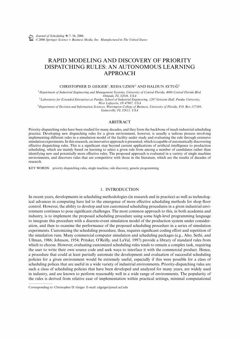
A number of different approaches have been developed under the name of rule discovery systems including rule-based classifier systems that construct “if-then” production rules through induction (Holland, 1986; Hollandand Reitman, 1978). Olafsson (2003) uses decision-tree induction and data-mining principles to generatescheduling rules within the production environment. These rule-discovery systems attempt to model theprocess of discovering new concepts through direct search of the space of concepts defined by symbolicdescriptions of those concepts. The architecture of SCRUPLES embodies that of the basic learning systemmodel (Russell and Norvig, 1995), which consists of two primary components—a reasoning mechanism anda performance evaluator, represents the problem domain, as shown in Figure 1. The reasoning mechanismis the adaptive component that implements the strategy by which new solutions are created and the solutionspace is searched.

Our system starts with a candidate set of rules that are either randomly or heuristically generated. Theserules are passed to the problem domain where the quality of each rule is assessed using one or more quan-titative measures of performance. In our system, this function is performed by a discrete-event simulationmodel that describes the production environment in which the rules are evaluated. The logic of the reasoningmechanism is independent of the mechanics of the evaluation procedure and requires only the numericaloutput measures from the performance evaluator to modify the solutions in the next generation. The valuesof the performance measures for all candidate rules are passed to the reasoning mechanism, where the next setof rules is constructed from the current high-performing rules using evolutionary search operators. This nextset of rules is then passed to the problem domain so that the performance of the new rules can be evaluated.This cycle is repeated until an acceptable level of rule performance is achieved.

Figure 1. Conceptual model of the proposed scheduling rule learning system.


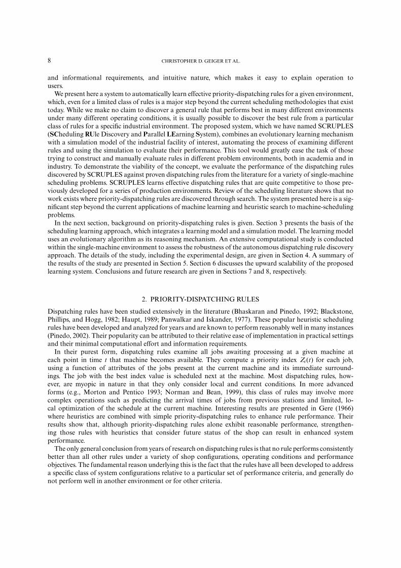
Figure 2. Four-stage cycle of evolutionary-based algorithms.

3.1. The discovery mechanism—An evolutionary-based search approach

The specific mechanism we use to explore the space of possible dispatching rules is evolutionary search.Evolutionary algorithms (EAs) are search procedures that attempt to emulate this natural phenomenon inartificial systems as a method to solve optimization problems. They maintain a population of encoded solutionstructures representing potential behavior of the system. This population of solutions is a sample of points inthe solution search space, allowing EAs to simultaneously allocate search effort to many regions of the searchspace in parallel.

The general procedure of an EA can be viewed conceptually as a four-stage cycle, as shown in Figure 2. Thealgorithm begins in Stage 1 with an initial population of solution structures that are created either randomly orheuristically. Again, the structures in this set represent a sampling of points in the space of potential solutionsto the given optimization problem. This is a fundamental difference between EAs and other search proceduressuch as blind search, hill climbing, simulated annealing or tabu search, which make incremental changes to asingle-solution structure in the search space (Reeves, 1993). Each solution in the set is then decoded in Stage 2so that its performance (fitness) can be evaluated. At Stage 3, a selection mechanism uses these fitness valuesto choose a subset of structures for reproduction at Stage 4, generating a new set of candidate structures. Overa number of cycles, the population as a whole contains those individuals who perform the best (i.e., are themost fit) in their environment. See Back and Schwefel (1993) for an overview of the different varieties of theseevolutionary-based algorithms. A genetic algorithm (GA), which is the best known and most widely used ofevolutionary heuristic search algorithms, is used in this research.

The power and relative success of GAs as the primary solution discovery heuristic in autonomous learn-ing systems has led to their application to production scheduling, often with valuable results (Davis, 1991;De Jong, 1988; Goldberg, 1989). Research on GAs in scheduling shows that they have been successfullyused to discover permutations of sets of jobs and resources (e.g., Bagchi, 1991; Cheng, 1999; Della, 1995;Dimopoulos and Zalzala, 1999; Mattfeld, 1996; Norman and Bean, 1999; Storer, Wu, and Park, 1992).Norman and Bean (1997) successfully apply the random key solution representation in order to generatefeasible job sequences within the job shop scheduling environment. Storer, Wu, and Vaccari (1992) presenta unique approach that uses local search procedures to search both the problem space and the heuristicspace to build job sequences. They use a simple hill-climbing procedure to illustrate the proposed method.They go on to discuss how the approach is amenable to GAs. Genetic algorithms have also been usedto select the best rule from a list of scheduling rules (e.g., Chiu and Yih, 1995; Lee, 1997; Pierreval andMebarki, 1997; Piramuthu, Raman, and Shaw, 1994; Shaw, Park, and Raman, 1992). GAs have also suc-cessfully learned executable computer programs (e.g., Banzhaf et al., 1998; De Jong, 1987; Koza, 1992). Thisarea of research is a promising new field of evolutionary heuristic search that transfers the genetic searchparadigm to the space of computer programs. It is this idea of learning computer programs that we drawupon for the discovery of effective dispatching rules. Specifically, we use the ideas of genetic programming(GP), an extension of the GA search paradigm and explores the space of computer programs, which are


represented as rooted trees. Each tree is composed of functions and terminal primitives relevant to a par-ticular problem domain, and can be of varying length. The set of available primitives is defined a priori.The search space is made up of all of the varied-length trees that can be constructed using the primitiveset.

Previous research on GP indicates its applicability to many different real-world applications, where theproblem domain can be interpreted as a program discovery problem (Koza, 1992). Genetic programminguses the optimization techniques of genetic algorithms to evolve computer programs, mimicking humanprogrammers constructing programs by progressively re-writing them. We apply the idea of automaticallylearning programs to the discovery of effective dispatching rules, basically by viewing each dispatchingrule as a program. In the next section, we define the learning environment as well as how solutions, i.e.,dispatching rules, that are discovered by the search procedure are encoded into the tree-based representa-tion. Dimopoulos and Zalzala (1999) use GP to build sequencing policies that combine known sequenc-ing rules (e.g., EDD, SPT, MON). They do not, however, use fundamental attributes to construct thesepolicies.

The choice of primitives is a crucial component of an effective GP algorithm. These primitives are the basicconstructs available to the GP that are assembled at the start of the search and are modified during its progress.GPs use this predefined set of primitives to discover possible solutions to the problem at hand. The set ofprimitives is grouped into two subsets: a set of relational and conditional functions, F, and a set of terminals, T.The set of terminals is usually problem-specific variables or numeric constants. The set of all possible solutionsdiscovered using the GP is the set of all possible solutions that can be represented using C, where C = F ∪T. Inchoosing the primitive set, a primary tradeoff involves the expressivity of the primitives versus the size of thesearch space. The expressivity of the primitive set is a measure of what fraction of all possible solutions can begenerated by combining the primitives in all possible manners, which is clearly a major factor in how general aprogram can be discovered. Hence, the size of the search space usually grows exponentially as a function of thenumber of primitives. On the other hand, a limited set of primitives generates a smaller search space, making thesearch more efficient but impossible to reach a good solution if that solution cannot be constructed using theprimitive set.

To illustrate this tradeoff, consider the concept of job slack, defined as si = di − pi − t, where, for job i, di

is its due date, pi is its processing time on the machine and t is the current time. Consider a primitive set thatincludes si but does not include its subcomponents di , pi and t. Then, the search is forced to build rules usingsi and it is unable to discover new relationships among its subcomponents. On the other hand, if si is notincluded in the primitive set but di , pi and t are, the GP will have the freedom to discover rules based on si aswell as other rules that can successfully solve the problem. However, because of the two extra primitives, thesearch may require additional effort to discover the rule that expresses job slack using the three more atomicattributes.

For many problems of interest, including scheduling problems, the complexity of an algorithm which willproduce the correct solution is not known a priori. GP has a key advantage over GAs in that it has the abilityto discover structures of varying lengths. This feature often makes genetic programming a preferred choiceover other discovery heuristics that use solution representation structures of fixed size, such as conventionalGAs and artificial neural networks.

3.2. Dispatching rule encoding

Recall that a dispatching rule is a logical expression that examines all jobs awaiting processing at a givenmachine at each time t that machine is available and computes, for each job i, a priority index Zi (t) usinga function of attributes of the entities in the current environment. The entities include not only the jobsthemselves but also the machines in the system and the system itself. The job with the best index value isprocessed next. Hence, the basic constructs of dispatching rules are the job, machine and system attributesused to compute the priority indices and the set of relational and conditional operators for combining them.Thus, the underlying solution representation we use consists of two components—a set of functions and


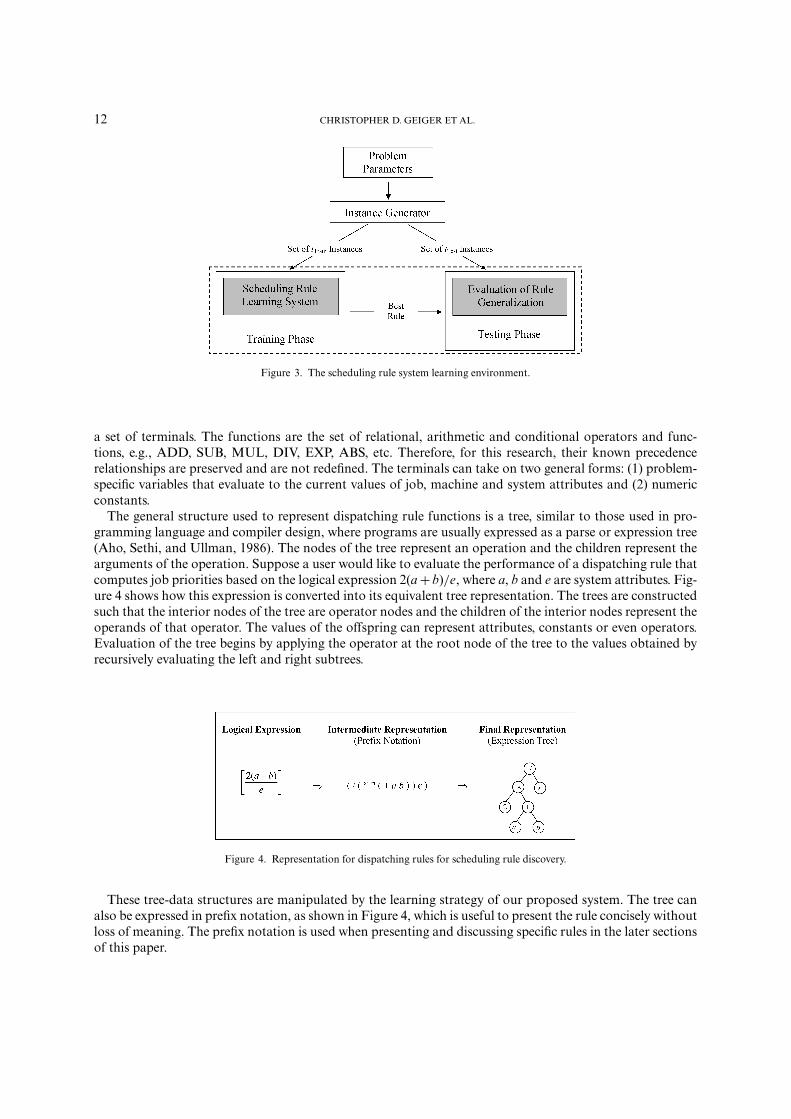
Figure 3. The scheduling rule system learning environment.

a set of terminals. The functions are the set of relational, arithmetic and conditional operators and func-tions, e.g., ADD, SUB, MUL, DIV, EXP, ABS, etc. Therefore, for this research, their known precedencerelationships are preserved and are not redefined. The terminals can take on two general forms: (1) problem-specific variables that evaluate to the current values of job, machine and system attributes and (2) numericconstants.

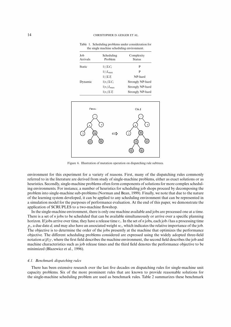
The general structure used to represent dispatching rule functions is a tree, similar to those used in pro-gramming language and compiler design, where programs are usually expressed as a parse or expression tree(Aho, Sethi, and Ullman, 1986). The nodes of the tree represent an operation and the children represent thearguments of the operation. Suppose a user would like to evaluate the performance of a dispatching rule thatcomputes job priorities based on the logical expression 2(a + b)/e, where a, b and e are system attributes. Fig-ure 4 shows how this expression is converted into its equivalent tree representation. The trees are constructedsuch that the interior nodes of the tree are operator nodes and the children of the interior nodes represent theoperands of that operator. The values of the offspring can represent attributes, constants or even operators.Evaluation of the tree begins by applying the operator at the root node of the tree to the values obtained byrecursively evaluating the left and right subtrees.

Figure 4. Representation for dispatching rules for scheduling rule discovery.

These tree-data structures are manipulated by the learning strategy of our proposed system. The tree canalso be expressed in prefix notation, as shown in Figure 4, which is useful to present the rule concisely withoutloss of meaning. The prefix notation is used when presenting and discussing specific rules in the later sectionsof this paper.


3.3. Scheduling rule search operators

3.3.1. CrossoverThe learning system utilizes an operation similar to the crossover operation of the conventional genetic

algorithm to create new solutions. Crossover begins by choosing two trees from the current population ofrules using the selection mechanism shown in Figure 5. Once each “parent” has been identified, a subtree ineach parent rule is selected at random. The randomly chosen subtrees are those with shaded nodes shown inthe figure. These subtrees are then swapped, creating two more individual trees (“children”). These child rulespossess information from each parent rule and provide new points in the dispatching rule search space forfurther testing. Note that by swapping subtrees during crossover as described here, we ensure that syntacticallyvalid offspring are produced.

Figure 5. Illustration of crossover operation on dispatching rule subtrees.

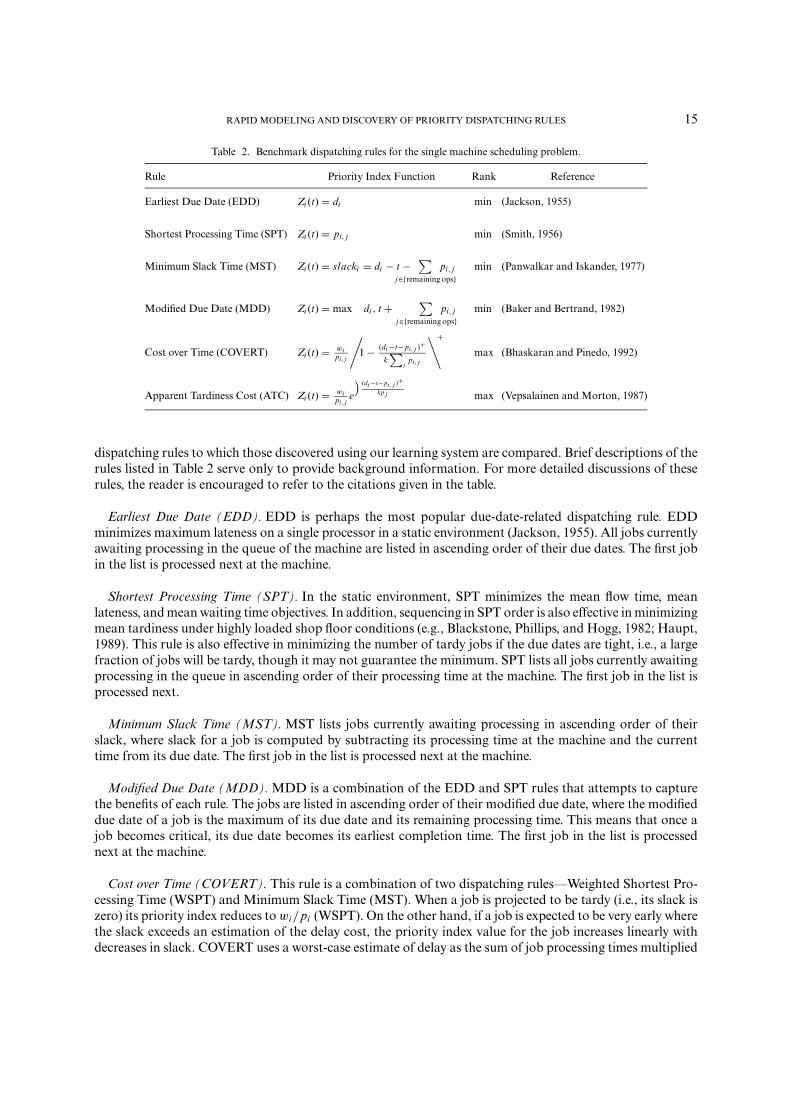
3.3.2. MutationThe mutation operation involves randomly selecting a subtree within a parent rule that has been selected for

reproduction and replacing it with a randomly generated subtree. The generated subtree is created by randomlyselecting primitives from the combined set of primitives C. Figure 6 illustrates this operation. The shadednodes represent the subtree that undergoes mutation. Similar to the genetic algorithm, mutation is considereda secondary operation in this work. Its purpose is to allow exploration of the search space by reintroducingdiversity into the population that may have been lost so that the search process does not converge to alocal optimum. The mutation operation as described here also ensures that syntacticallyvalid offspring areproduced.

4. EVALUATION OF PERFORMANCE OF THE SCHEDULING RULELEARNING SYSTEM

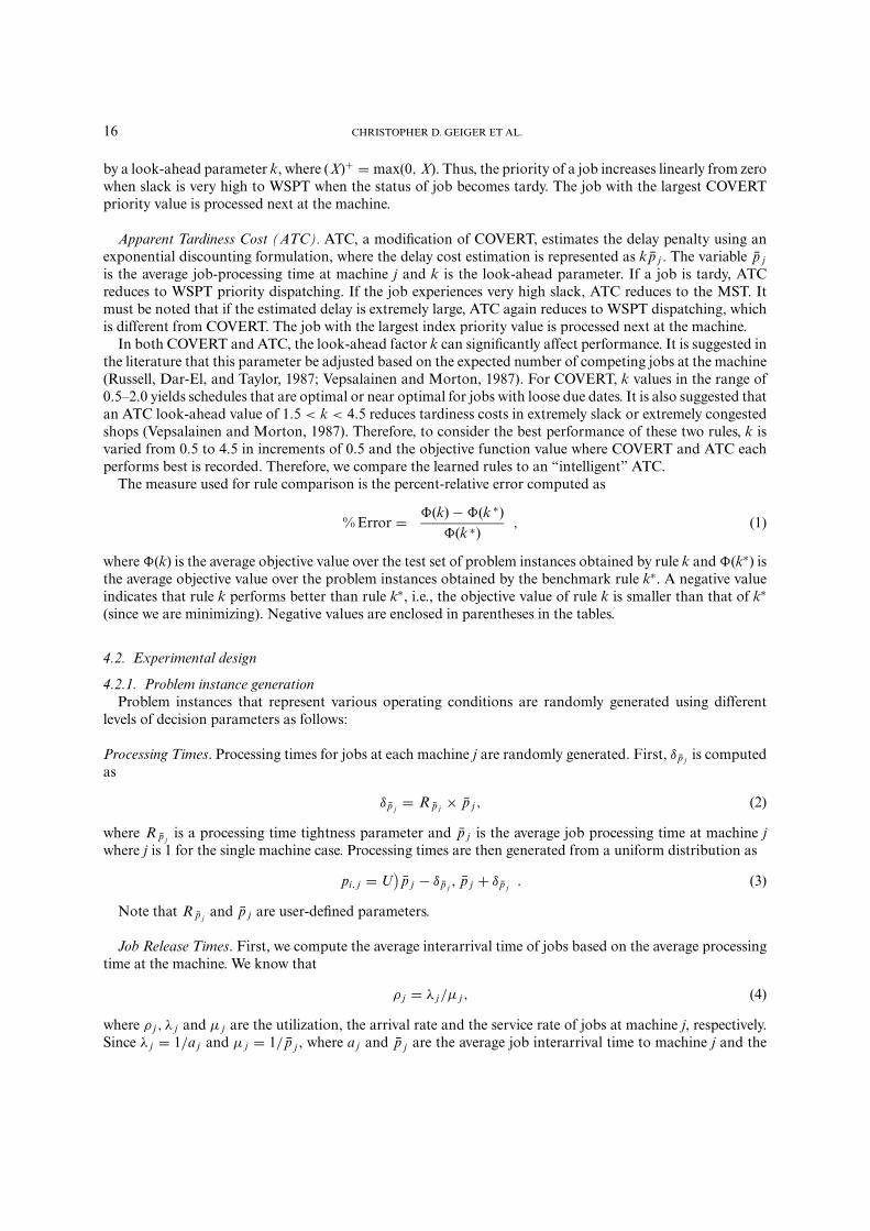
We now examine the learning system by applying it to a set of single machine scheduling problems of varyingdegrees of tractability. Table 1 lists the six scheduling problems addressed in this analysis. In this work, ageneral approach is presented that can be used in both static and dynamic scheduling environments. In staticscheduling problems, all jobs to be scheduled are available simultaneously at the start of the planning horizon.Dynamic scheduling problems involve jobs arriving over time during the planning horizon. Static problemsare considered because some of them are often solvable exactly in polynomial time, using dispatching rules.Dynamic problems often represent a more difficult scheduling environment. We choose the single-machine


Table 1. Scheduling problems under consideration forthe single machine scheduling environment.

Job Scheduling ComplexityArrivals Problem Status

Static 1| |�Ci P

1| |Lmax P

1| |�Ti NP-hard

Dynamic 1|ri |�Ci Strongly NP-hard

1|ri |Lmax Strongly NP-hard

1|ri |�Ti Strongly NP-hard

Figure 6. Illustration of mutation operation on dispatching rule subtrees.

environment for this experiment for a variety of reasons. First, many of the dispatching rules commonlyreferred to in the literature are derived from study of single-machine problems, either as exact solutions or asheuristics. Secondly, single-machine problems often form components of solutions for more complex schedul-ing environments. For instance, a number of heuristics for scheduling job shops proceed by decomposing theproblem into single-machine sub-problems (Norman and Bean, 1999). Finally, we note that due to the natureof the learning system developed, it can be applied to any scheduling environment that can be represented ina simulation model for the purposes of performance evaluation. At the end of this paper, we demonstrate theapplication of SCRUPLES to a two-machine flowshop.

In the single-machine environment, there is only one machine available and jobs are processed one at a time.There is a set of n jobs to be scheduled that can be available simultaneously or arrive over a specific planninghorizon. If jobs arrive over time, they have a release time ri . In the set of n jobs, each job i has a processing timepi , a due date di and may also have an associated weight wi , which indicates the relative importance of the job.The objective is to determine the order of the jobs presently at the machine that optimizes the performanceobjective. The different scheduling problems considered are expressed using the widely adopted three-fieldnotation α|β|γ , where the first field describes the machine environment, the second field describes the job andmachine characteristics such as job release times and the third field denotes the performance objective to beminimized (Blazewicz et al., 1996).

4.1. Benchmark dispatching rules

There has been extensive research over the last five decades on dispatching rules for single-machine unitcapacity problems. Six of the more prominent rules that are known to provide reasonable solutions forthe single-machine scheduling problem are used as benchmark rules. Table 2 summarizes these benchmark


Table 2. Benchmark dispatching rules for the single machine scheduling problem.

Rule Priority Index Function Rank Reference

Earliest Due Date (EDD) Zi (t) = di min (Jackson, 1955)

Shortest Processing Time (SPT) Zi (t) = pi, j min (Smith, 1956)

Minimum Slack Time (MST) Zi (t) = slacki = di − t −∑

j∈{remaining ops}pi, j min (Panwalkar and Iskander, 1977)

Modified Due Date (MDD) Zi (t) = max di , t +∑

j∈{remaining ops}pi, j min (Baker and Bertrand, 1982)

Cost over Time (COVERT) Zi (t) = wipi, j

/1 − (di −t−pi, j )+

k∑

ipi, j

∖+max (Bhaskaran and Pinedo, 1992)

Apparent Tardiness Cost (ATC) Zi (t) = wipi, j

e

)(di −t−pi, j )+

kp j max (Vepsalainen and Morton, 1987)

dispatching rules to which those discovered using our learning system are compared. Brief descriptions of therules listed in Table 2 serve only to provide background information. For more detailed discussions of theserules, the reader is encouraged to refer to the citations given in the table.

Earliest Due Date (EDD). EDD is perhaps the most popular due-date-related dispatching rule. EDDminimizes maximum lateness on a single processor in a static environment (Jackson, 1955). All jobs currentlyawaiting processing in the queue of the machine are listed in ascending order of their due dates. The first jobin the list is processed next at the machine.

Shortest Processing Time (SPT). In the static environment, SPT minimizes the mean flow time, meanlateness, and mean waiting time objectives. In addition, sequencing in SPT order is also effective in minimizingmean tardiness under highly loaded shop floor conditions (e.g., Blackstone, Phillips, and Hogg, 1982; Haupt,1989). This rule is also effective in minimizing the number of tardy jobs if the due dates are tight, i.e., a largefraction of jobs will be tardy, though it may not guarantee the minimum. SPT lists all jobs currently awaitingprocessing in the queue in ascending order of their processing time at the machine. The first job in the list isprocessed next.

Minimum Slack Time (MST). MST lists jobs currently awaiting processing in ascending order of theirslack, where slack for a job is computed by subtracting its processing time at the machine and the currenttime from its due date. The first job in the list is processed next at the machine.

Modified Due Date (MDD). MDD is a combination of the EDD and SPT rules that attempts to capturethe benefits of each rule. The jobs are listed in ascending order of their modified due date, where the modifieddue date of a job is the maximum of its due date and its remaining processing time. This means that once ajob becomes critical, its due date becomes its earliest completion time. The first job in the list is processednext at the machine.

Cost over Time (COVERT). This rule is a combination of two dispatching rules—Weighted Shortest Pro-cessing Time (WSPT) and Minimum Slack Time (MST). When a job is projected to be tardy (i.e., its slack iszero) its priority index reduces to wi/pi (WSPT). On the other hand, if a job is expected to be very early wherethe slack exceeds an estimation of the delay cost, the priority index value for the job increases linearly withdecreases in slack. COVERT uses a worst-case estimate of delay as the sum of job processing times multiplied


by a look-ahead parameter k, where (X)+ = max(0, X). Thus, the priority of a job increases linearly from zerowhen slack is very high to WSPT when the status of job becomes tardy. The job with the largest COVERTpriority value is processed next at the machine.

Apparent Tardiness Cost (ATC). ATC, a modification of COVERT, estimates the delay penalty using anexponential discounting formulation, where the delay cost estimation is represented as kp j . The variable p j

is the average job-processing time at machine j and k is the look-ahead parameter. If a job is tardy, ATCreduces to WSPT priority dispatching. If the job experiences very high slack, ATC reduces to the MST. Itmust be noted that if the estimated delay is extremely large, ATC again reduces to WSPT dispatching, whichis different from COVERT. The job with the largest index priority value is processed next at the machine.

In both COVERT and ATC, the look-ahead factor k can significantly affect performance. It is suggested inthe literature that this parameter be adjusted based on the expected number of competing jobs at the machine(Russell, Dar-El, and Taylor, 1987; Vepsalainen and Morton, 1987). For COVERT, k values in the range of0.5–2.0 yields schedules that are optimal or near optimal for jobs with loose due dates. It is also suggested thatan ATC look-ahead value of 1.5 < k < 4.5 reduces tardiness costs in extremely slack or extremely congestedshops (Vepsalainen and Morton, 1987). Therefore, to consider the best performance of these two rules, k isvaried from 0.5 to 4.5 in increments of 0.5 and the objective function value where COVERT and ATC eachperforms best is recorded. Therefore, we compare the learned rules to an “intelligent” ATC.

The measure used for rule comparison is the percent-relative error computed as

% Error = �(k) − �(k ∗)�(k ∗)

, (1)

where �(k) is the average objective value over the test set of problem instances obtained by rule k and �(k∗) isthe average objective value over the problem instances obtained by the benchmark rule k∗. A negative valueindicates that rule k performs better than rule k∗, i.e., the objective value of rule k is smaller than that of k∗

(since we are minimizing). Negative values are enclosed in parentheses in the tables.

4.2. Experimental design

4.2.1. Problem instance generationProblem instances that represent various operating conditions are randomly generated using different

levels of decision parameters as follows:

Processing Times. Processing times for jobs at each machine j are randomly generated. First, δ p j is computedas

δ p j= R p j × p j , (2)

where R p jis a processing time tightness parameter and p j is the average job processing time at machine j

where j is 1 for the single machine case. Processing times are then generated from a uniform distribution as

pi, j = U)

p j − δ p j, p j + δ p j

. (3)

Note that R p jand p j are user-defined parameters.

Job Release Times. First, we compute the average interarrival time of jobs based on the average processingtime at the machine. We know that

ρ j = λ j/µ j , (4)

where ρ j , λ j and µ j are the utilization, the arrival rate and the service rate of jobs at machine j, respectively.Since λ j = 1/a j and µ j = 1/ p j , where a j and p j are the average job interarrival time to machine j and the


average job processing time at machine j, respectively, then

a j = p j/ρ j . (5)

Considering the desired level of variability of the job interarrival time and the desired level of machineutilization, job release times are then assigned using an approach similar to that used for generating processingtimes. First, δa j is computed as

δa j = Ra j × a j , (6)

where Ra j is a job interarrival time tightness parameter and a j is the average interarrival time for machine j,respectively. Release times are generated from a uniform distribution using the two equations

ri = U)a j − δa j , a j + δa j (7)

ri = ri−1 + U(a j − δa j , a j + δa j ) for i = 2, . . . , n. (8)

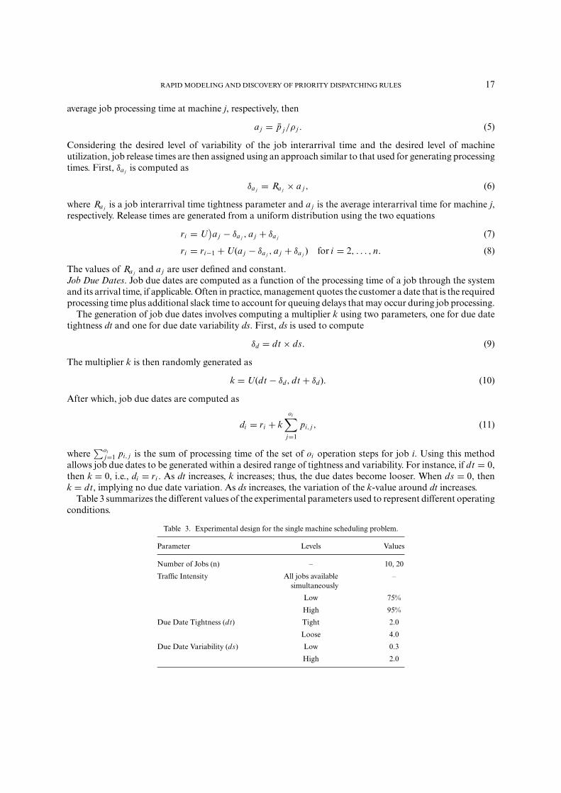
The values of Ra j and a j are user defined and constant.Job Due Dates. Job due dates are computed as a function of the processing time of a job through the systemand its arrival time, if applicable. Often in practice, management quotes the customer a date that is the requiredprocessing time plus additional slack time to account for queuing delays that may occur during job processing.

The generation of job due dates involves computing a multiplier k using two parameters, one for due datetightness dt and one for due date variability ds. First, ds is used to compute

δd = dt × ds. (9)

The multiplier k is then randomly generated as

k = U(dt − δd , dt + δd ). (10)

After which, job due dates are computed as

di = ri + koi∑

j=1

pi, j , (11)

where∑oi

j=1 pi, j is the sum of processing time of the set of oi operation steps for job i. Using this methodallows job due dates to be generated within a desired range of tightness and variability. For instance, if dt = 0,then k = 0, i.e., di = ri . As dt increases, k increases; thus, the due dates become looser. When ds = 0, thenk = dt, implying no due date variation. As ds increases, the variation of the k-value around dt increases.

Table 3 summarizes the different values of the experimental parameters used to represent different operatingconditions.

Table 3. Experimental design for the single machine scheduling problem.

Parameter Levels Values

Number of Jobs (n) – 10, 20

Traffic Intensity All jobs available –simultaneously

Low 75%

High 95%

Due Date Tightness (dt) Tight 2.0

Loose 4.0

Due Date Variability (ds) Low 0.3

High 2.0


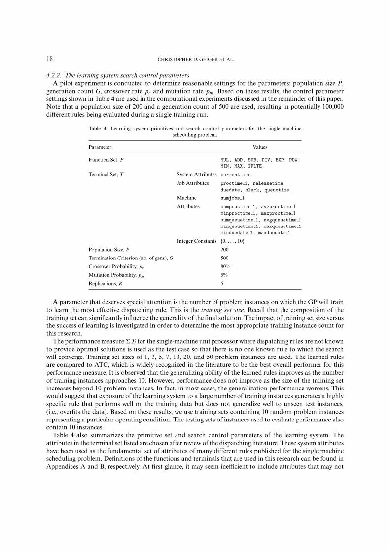
4.2.2. The learning system search control parametersA pilot experiment is conducted to determine reasonable settings for the parameters: population size P,

generation count G, crossover rate pc and mutation rate pm. Based on these results, the control parametersettings shown in Table 4 are used in the computational experiments discussed in the remainder of this paper.Note that a population size of 200 and a generation count of 500 are used, resulting in potentially 100,000different rules being evaluated during a single training run.

Table 4. Learning system primitives and search control parameters for the single machinescheduling problem.

Parameter Values

Function Set, F MUL, ADD, SUB, DIV, EXP, POW,MIN, MAX, IFLTE

Terminal Set, T System Attributes currenttime

Job Attributes proctime 1, releasetimeduedate, slack, queuetime

Machine sumjobs 1

Attributes sumproctime 1, avgproctime 1minproctime 1, maxproctime 1sumqueuetime 1, avgqueuetime 1minqueuetime 1, maxqueuetime 1minduedate 1, maxduedate 1

Integer Constants {0, . . . , 10}Population Size, P 200

Termination Criterion (no. of gens), G 500

Crossover Probability, pc 80%

Mutation Probability, pm 5%

Replications, R 5

A parameter that deserves special attention is the number of problem instances on which the GP will trainto learn the most effective dispatching rule. This is the training set size. Recall that the composition of thetraining set can significantly influence the generality of the final solution. The impact of training set size versusthe success of learning is investigated in order to determine the most appropriate training instance count forthis research.

The performance measure �Ti for the single-machine unit processor where dispatching rules are not knownto provide optimal solutions is used as the test case so that there is no one known rule to which the searchwill converge. Training set sizes of 1, 3, 5, 7, 10, 20, and 50 problem instances are used. The learned rulesare compared to ATC, which is widely recognized in the literature to be the best overall performer for thisperformance measure. It is observed that the generalizing ability of the learned rules improves as the numberof training instances approaches 10. However, performance does not improve as the size of the training setincreases beyond 10 problem instances. In fact, in most cases, the generalization performance worsens. Thiswould suggest that exposure of the learning system to a large number of training instances generates a highlyspecific rule that performs well on the training data but does not generalize well to unseen test instances,(i.e., overfits the data). Based on these results, we use training sets containing 10 random problem instancesrepresenting a particular operating condition. The testing sets of instances used to evaluate performance alsocontain 10 instances.

Table 4 also summarizes the primitive set and search control parameters of the learning system. Theattributes in the terminal set listed are chosen after review of the dispatching literature. These system attributeshave been used as the fundamental set of attributes of many different rules published for the single machinescheduling problem. Definitions of the functions and terminals that are used in this research can be found inAppendices A and B, respectively. At first glance, it may seem inefficient to include attributes that may not


be relevant to a particular objective function. For instance, including job processing time when attempting todiscover rules for the 1‖Lmax problem may seem ill-advised, since we know that the EDD rule is optimal for thisproblem and this does not consider processing times at all. However, by making the entire list of attributesavailable to the system for the six scheduling problems, our hope is that new and interesting relationshipsamong attributes will emerge, which may not be obvious. The system also ought to be smart enough todisregard irrelevant attributes.

We run the learning system for five replications. For each replication, the search is run from a differentinitial population of points in the search space. We use this multi-start search approach to develop insightinto the inherent variability of the learning procedure due to its randomized nature.

5. EXPERIMENTAL RESULTS

In discussing the performance of all dispatching rules under the different operating scenarios, we use thetriple <n, dt, ds> to represent a scenario. For example, <10, 2.0, 0.3> represents the production scenariowhere there are 10 jobs to be scheduled with tight due dates and low due date variability. We insert “∗” if thespecific parameter in the representation is not relevant to the discussion. For example, <∗, 2.0,∗> representall instances with tight due date conditions, regardless of the variation of due dates and the number of jobsto be scheduled.

5.1. Minimizing �Ci

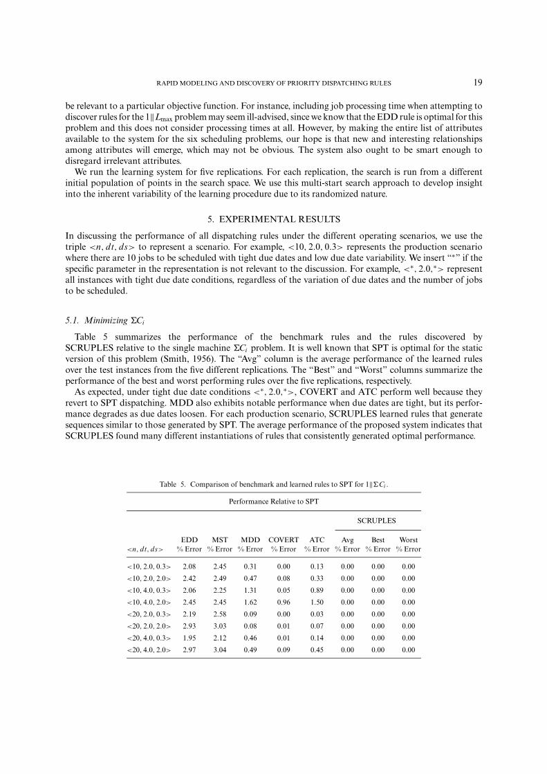
Table 5 summarizes the performance of the benchmark rules and the rules discovered bySCRUPLES relative to the single machine �Ci problem. It is well known that SPT is optimal for the staticversion of this problem (Smith, 1956). The “Avg” column is the average performance of the learned rulesover the test instances from the five different replications. The “Best” and “Worst” columns summarize theperformance of the best and worst performing rules over the five replications, respectively.

As expected, under tight due date conditions <∗, 2.0,∗>, COVERT and ATC perform well because theyrevert to SPT dispatching. MDD also exhibits notable performance when due dates are tight, but its perfor-mance degrades as due dates loosen. For each production scenario, SCRUPLES learned rules that generatesequences similar to those generated by SPT. The average performance of the proposed system indicates thatSCRUPLES found many different instantiations of rules that consistently generated optimal performance.

Table 5. Comparison of benchmark and learned rules to SPT for 1‖�Ci .

Performance Relative to SPT

SCRUPLES

EDD MST MDD COVERT ATC Avg Best Worst<n, dt, ds> % Error % Error % Error % Error % Error % Error % Error % Error

<10, 2.0, 0.3> 2.08 2.45 0.31 0.00 0.13 0.00 0.00 0.00

<10, 2.0, 2.0> 2.42 2.49 0.47 0.08 0.33 0.00 0.00 0.00

<10, 4.0, 0.3> 2.06 2.25 1.31 0.05 0.89 0.00 0.00 0.00

<10, 4.0, 2.0> 2.45 2.45 1.62 0.96 1.50 0.00 0.00 0.00

<20, 2.0, 0.3> 2.19 2.58 0.09 0.00 0.03 0.00 0.00 0.00

<20, 2.0, 2.0> 2.93 3.03 0.08 0.01 0.07 0.00 0.00 0.00

<20, 4.0, 0.3> 1.95 2.12 0.46 0.01 0.14 0.00 0.00 0.00

<20, 4.0, 2.0> 2.97 3.04 0.49 0.09 0.45 0.00 0.00 0.00


As mentioned earlier, the specific rules are not as important as the relationships among the assembledattributes that emerge. However, the learning system often assembles relevant and irrelevant primitives andsub-expressions to construct the different rules. We define irrelevant primitives and sub-expressions as thosethat do not directly affect the priority value of the learned rule when removed from the rule. In other words,the removal of the primitives and sub-expressions do not change the original sequencing of the jobs. Giventhis occurrence, there is a need to simplify the rules to make them more intelligible so that the relationshipsamong the attributes are identifiable.

Examining the learned rules shows that sequencing the jobs in increasing order of their processing timeat the machine generates the best performance. Many of the rules have proctime 1 embedded within them.In other instances, the discovered rules contain constants that assume the same value across all jobs beingprioritized at the machine. Therefore, these constants can be removed from the priority index function.When these constants are removed from the discovered dispatching rules, the result is sequencing in SPTorder. For example, the SCRUPLES approach discovers the following priority index function for the scenario<10, 4.0, 0.3> in replication 4:

(ADD proctime 1 (MAX (NEG sumjobs 1) sumqueuetime 1)).

Closer examination reveals that the sub-expression

(MAX (NEG sumjobs 1) sumqueuetime 1)

computes to the same value for all jobs being prioritized. Therefore, this expression is equivalent to

(ADD proctime 1 constant),

which is equivalent to SPT. This indicates the need for further research to try to prevent this from occurringwithout biasing or limiting the ability of the system to discover new rules.

Similar to the static version, all rules, including those that are learned, are compared to SPT for the dynamiccase. This rule has repeatedly been shown to yield high-quality solutions (Chang, Sueyoshi, and Sullivan, 1996)and has been proven to be asymptotically optimal. Tables 6 and 7, which summarize rule performance formachine utilizations of 75 and 95%, respectively, show that SPT demonstrates superior performance to allother rules. In addition, the performance of all other benchmark rules degrades slightly as the machineutilization increases. However, the rules learned using SCRUPLES remain competitive with SPT over allscenarios even as machine utilization increases.

Table 6. Comparison of benchmark and learned rules to SPT for 1|ri |�Ci when machine uti-lization is 75%.


SCRUPLES


<10, 2.0, 0.3> 0.45 0.70 0.12 0.01 0.02 0.00 0.00 0.00

<10, 2.0, 2.0> 0.37 0.54 0.06 0.03 0.03 0.00 0.00 0.00

<10, 4.0, 0.3> 0.02 0.02 0.02 0.00 0.02 0.00 0.00 0.00

<10, 4.0, 2.0> 0.10 0.10 0.10 0.04 0.00 0.00 0.00 0.00

<20, 2.0, 0.3> 0.45 0.52 0.05 0.00 0.01 0.01 0.00 0.04

<20, 2.0, 2.0> 0.64 0.64 0.46 0.07 0.16 0.09 0.01 0.27

<20, 4.0, 0.3> 0.09 0.12 0.09 0.04 0.05 0.01 0.00 0.02

<20, 4.0, 2.0> 0.36 0.36 0.33 0.19 0.22 0.00 0.00 0.00


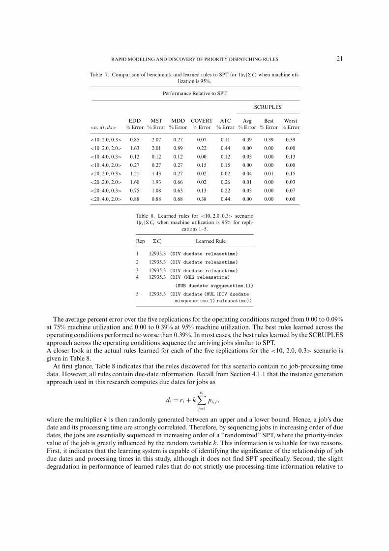
Table 7. Comparison of benchmark and learned rules to SPT for 1|ri |�Ci when machine uti-lization is 95%.


SCRUPLES


<10, 2.0, 0.3> 0.85 2.07 0.27 0.07 0.11 0.39 0.39 0.39

<10, 2.0, 2.0> 1.63 2.01 0.89 0.22 0.44 0.00 0.00 0.00

<10, 4.0, 0.3> 0.12 0.12 0.12 0.00 0.12 0.03 0.00 0.13

<10, 4.0, 2.0> 0.27 0.27 0.27 0.15 0.15 0.00 0.00 0.00

<20, 2.0, 0.3> 1.21 1.43 0.27 0.02 0.02 0.04 0.01 0.15

<20, 2.0, 2.0> 1.60 1.93 0.66 0.02 0.26 0.01 0.00 0.03

<20, 4.0, 0.3> 0.75 1.08 0.63 0.13 0.22 0.03 0.00 0.07

<20, 4.0, 2.0> 0.88 0.88 0.68 0.38 0.44 0.00 0.00 0.00

Table 8. Learned rules for <10, 2.0, 0.3> scenario1|ri |�Ci when machine utilization is 95% for repli-

cations 1–5.

Rep �Ci Learned Rule

1 12935.3 (DIV duedate releasetime)

2 12935.3 (DIV duedate releasetime)

3 12935.3 (DIV duedate releasetime)4 12935.3 (DIV (NEG releasetime)

(SUB duedate avgqueuetime 1))

5 12935.3 (DIV duedate (MUL (DIV duedateminqueuetime 1) releasetime))

The average percent error over the five replications for the operating conditions ranged from 0.00 to 0.09%at 75% machine utilization and 0.00 to 0.39% at 95% machine utilization. The best rules learned across theoperating conditions performed no worse than 0.39%. In most cases, the best rules learned by the SCRUPLESapproach across the operating conditions sequence the arriving jobs similar to SPT.A closer look at the actual rules learned for each of the five replications for the <10, 2.0, 0.3> scenario isgiven in Table 8.

At first glance, Table 8 indicates that the rules discovered for this scenario contain no job-processing timedata. However, all rules contain due-date information. Recall from Section 4.1.1 that the instance generationapproach used in this research computes due dates for jobs as

di = ri + koi∑

j=1

pi, j ,

where the multiplier k is then randomly generated between an upper and a lower bound. Hence, a job’s duedate and its processing time are strongly correlated. Therefore, by sequencing jobs in increasing order of duedates, the jobs are essentially sequenced in increasing order of a “randomized” SPT, where the priority-indexvalue of the job is greatly influenced by the random variable k. This information is valuable for two reasons.First, it indicates that the learning system is capable of identifying the significance of the relationship of jobdue dates and processing times in this study, although it does not find SPT specifically. Second, the slightdegradation in performance of learned rules that do not strictly use processing-time information relative to


SPT gives an indication of the importance of this information for the flow-time based performance objective�Ci .

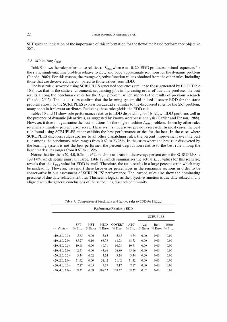
5.2. Minimizing Lmax

Table 9 shows the rule performance relative to Lmax when n = 10, 20. EDD produces optimal sequences forthe static single-machine problem relative to Lmax and good approximate solutions for the dynamic problem(Pinedo, 2002). For this reason, the average objective function values obtained from the other rules, includingthose that are discovered, are compared to those values from EDD.

The best rule discovered using SCRUPLES generated sequences similar to those generated by EDD. Table10 shows that in the static environment, sequencing jobs in increasing order of due date produces the bestresults among the benchmark rules for the Lmax problem, which supports the results of previous research(Pinedo, 2002). The actual rules confirm that the learning system did indeed discover EDD for the staticproblem shown by the SCRUPLES expression duedate. Similar to the discovered rules for the �Ci problem,many contain irrelevant attributes. Reducing these rules yields the EDD rule.

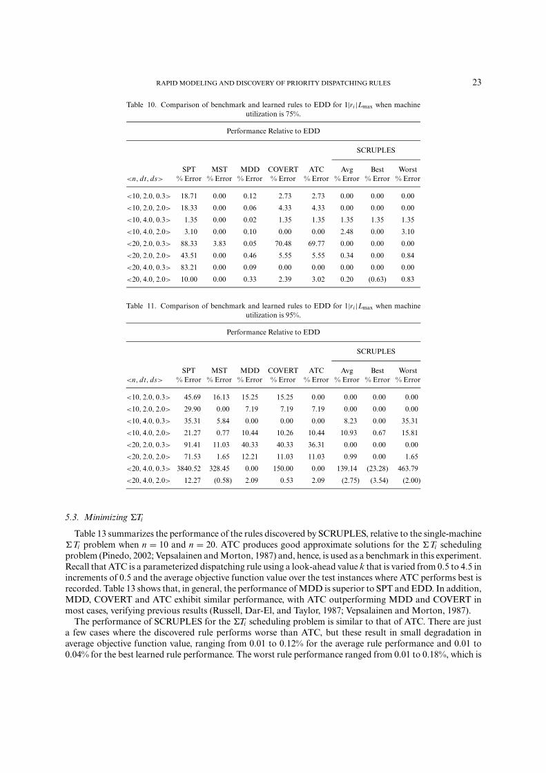
Tables 10 and 11 show rule performance relative to EDD dispatching for 1|ri |Lmax. EDD performs well inthe presence of dynamic job arrivals, as suggested by known worst-case analysis (Carlier and Pinson, 1988).However, it does not guarantee the best solutions for the single-machine Lmax problem, shown by other rulesreceiving a negative percent error score. These results underscore previous research. In most cases, the bestrule found using SCRUPLES either exhibits the best performance or ties for the best. In the cases whereSCRUPLES discovers rules superior to all other dispatching rules, the percent improvement over the bestrule among the benchmark rules ranges from 0.63 to 23.28%. In the cases where the best rule discovered bythe learning system is not the best performer, the percent degradation relative to the best rule among thebenchmark rules ranges from 0.67 to 1.35%.

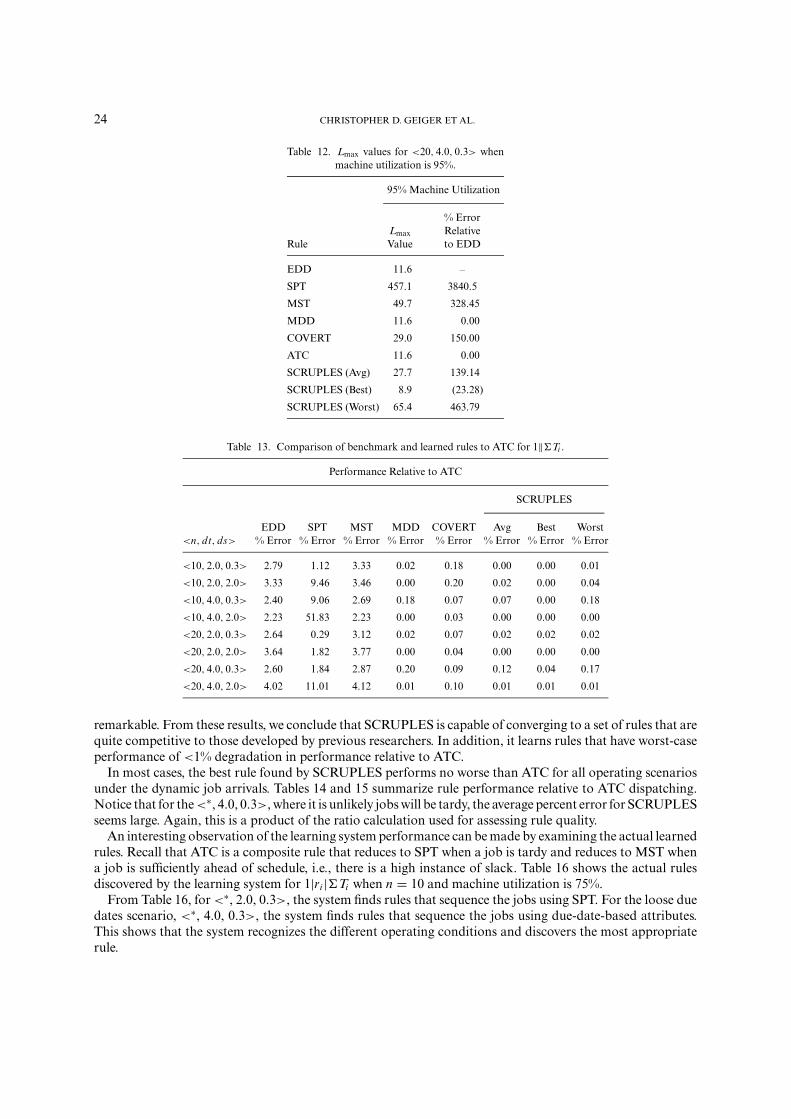
Notice that for the <20, 4.0, 0.3> at 95% machine utilization, the average percent error for SCRUPLES is139.14%, which seems unusually large. Table 12, which summarizes the actual Lmax values for this scenario,reveals that the Lmax value for EDD is small. Therefore, the ratio results in a large percent error, which maybe misleading. However, we report these large error percentages in the remaining sections in order to beconservative in our assessment of SCRUPLES’ performance. The learned rules also show the dominatingpresence of due date-related attributes. This seems logical, as the objective function is due-date-related and isaligned with the general conclusions of the scheduling research community.

Table 9. Comparison of benchmark and learned rules to EDD for 1‖Lmax.

Performance Relative to EDD

SCRUPLES

SPT MST MDD COVERT ATC Avg Best Worst<n, dt, ds> % Error % Error % Error % Error % Error % Error % Error % Error

<10, 2.0, 0.3> 5.65 0.06 5.65 5.65 4.74 0.00 0.00 0.00

<10, 2.0, 2.0> 85.27 0.16 68.73 68.73 68.73 0.00 0.00 0.00

<10, 4.0, 0.3> 19.68 0.00 10.71 10.78 10.71 0.00 0.00 0.00

<10, 4.0, 2.0> 142.51 0.00 43.66 56.89 43.66 0.00 0.00 0.00

<20, 2.0, 0.3> 3.34 0.02 3.34 3.34 3.34 0.00 0.00 0.00

<20, 2.0, 2.0> 31.42 0.00 31.42 31.42 31.42 0.00 0.00 0.00

<20, 4.0, 0.3> 7.17 0.05 7.17 7.17 7.17 0.00 0.00 0.00

<20, 4.0, 2.0> 108.22 0.09 108.22 108.22 108.22 0.02 0.00 0.09


Table 10. Comparison of benchmark and learned rules to EDD for 1|ri |Lmax when machineutilization is 75%.


SCRUPLES


<10, 2.0, 0.3> 18.71 0.00 0.12 2.73 2.73 0.00 0.00 0.00

<10, 2.0, 2.0> 18.33 0.00 0.06 4.33 4.33 0.00 0.00 0.00

<10, 4.0, 0.3> 1.35 0.00 0.02 1.35 1.35 1.35 1.35 1.35

<10, 4.0, 2.0> 3.10 0.00 0.10 0.00 0.00 2.48 0.00 3.10

<20, 2.0, 0.3> 88.33 3.83 0.05 70.48 69.77 0.00 0.00 0.00

<20, 2.0, 2.0> 43.51 0.00 0.46 5.55 5.55 0.34 0.00 0.84

<20, 4.0, 0.3> 83.21 0.00 0.09 0.00 0.00 0.00 0.00 0.00

<20, 4.0, 2.0> 10.00 0.00 0.33 2.39 3.02 0.20 (0.63) 0.83

Table 11. Comparison of benchmark and learned rules to EDD for 1|ri |Lmax when machineutilization is 95%.


SCRUPLES


<10, 2.0, 0.3> 45.69 16.13 15.25 15.25 0.00 0.00 0.00 0.00

<10, 2.0, 2.0> 29.90 0.00 7.19 7.19 7.19 0.00 0.00 0.00

<10, 4.0, 0.3> 35.31 5.84 0.00 0.00 0.00 8.23 0.00 35.31

<10, 4.0, 2.0> 21.27 0.77 10.44 10.26 10.44 10.93 0.67 15.81

<20, 2.0, 0.3> 91.41 11.03 40.33 40.33 36.31 0.00 0.00 0.00

<20, 2.0, 2.0> 71.53 1.65 12.21 11.03 11.03 0.99 0.00 1.65

<20, 4.0, 0.3> 3840.52 328.45 0.00 150.00 0.00 139.14 (23.28) 463.79

<20, 4.0, 2.0> 12.27 (0.58) 2.09 0.53 2.09 (2.75) (3.54) (2.00)

5.3. Minimizing �Ti

Table 13 summarizes the performance of the rules discovered by SCRUPLES, relative to the single-machine�Ti problem when n = 10 and n = 20. ATC produces good approximate solutions for the �Ti schedulingproblem (Pinedo, 2002; Vepsalainen and Morton, 1987) and, hence, is used as a benchmark in this experiment.Recall that ATC is a parameterized dispatching rule using a look-ahead value k that is varied from 0.5 to 4.5 inincrements of 0.5 and the average objective function value over the test instances where ATC performs best isrecorded. Table 13 shows that, in general, the performance of MDD is superior to SPT and EDD. In addition,MDD, COVERT and ATC exhibit similar performance, with ATC outperforming MDD and COVERT inmost cases, verifying previous results (Russell, Dar-El, and Taylor, 1987; Vepsalainen and Morton, 1987).

The performance of SCRUPLES for the �Ti scheduling problem is similar to that of ATC. There are justa few cases where the discovered rule performs worse than ATC, but these result in small degradation inaverage objective function value, ranging from 0.01 to 0.12% for the average rule performance and 0.01 to0.04% for the best learned rule performance. The worst rule performance ranged from 0.01 to 0.18%, which is


Table 12. Lmax values for <20, 4.0, 0.3> whenmachine utilization is 95%.

95% Machine Utilization

% ErrorLmax Relative

Rule Value to EDD

EDD 11.6 –

SPT 457.1 3840.5

MST 49.7 328.45

MDD 11.6 0.00

COVERT 29.0 150.00

ATC 11.6 0.00

SCRUPLES (Avg) 27.7 139.14

SCRUPLES (Best) 8.9 (23.28)

SCRUPLES (Worst) 65.4 463.79

Table 13. Comparison of benchmark and learned rules to ATC for 1‖�Ti .

Performance Relative to ATC

SCRUPLES

EDD SPT MST MDD COVERT Avg Best Worst<n, dt, ds> % Error % Error % Error % Error % Error % Error % Error % Error

<10, 2.0, 0.3> 2.79 1.12 3.33 0.02 0.18 0.00 0.00 0.01

<10, 2.0, 2.0> 3.33 9.46 3.46 0.00 0.20 0.02 0.00 0.04

<10, 4.0, 0.3> 2.40 9.06 2.69 0.18 0.07 0.07 0.00 0.18

<10, 4.0, 2.0> 2.23 51.83 2.23 0.00 0.03 0.00 0.00 0.00

<20, 2.0, 0.3> 2.64 0.29 3.12 0.02 0.07 0.02 0.02 0.02

<20, 2.0, 2.0> 3.64 1.82 3.77 0.00 0.04 0.00 0.00 0.00

<20, 4.0, 0.3> 2.60 1.84 2.87 0.20 0.09 0.12 0.04 0.17

<20, 4.0, 2.0> 4.02 11.01 4.12 0.01 0.10 0.01 0.01 0.01

remarkable. From these results, we conclude that SCRUPLES is capable of converging to a set of rules that arequite competitive to those developed by previous researchers. In addition, it learns rules that have worst-caseperformance of <1% degradation in performance relative to ATC.

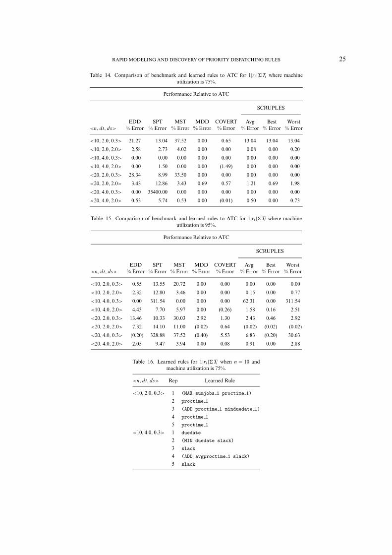
In most cases, the best rule found by SCRUPLES performs no worse than ATC for all operating scenariosunder the dynamic job arrivals. Tables 14 and 15 summarize rule performance relative to ATC dispatching.Notice that for the <∗, 4.0, 0.3>, where it is unlikely jobs will be tardy, the average percent error for SCRUPLESseems large. Again, this is a product of the ratio calculation used for assessing rule quality.

An interesting observation of the learning system performance can be made by examining the actual learnedrules. Recall that ATC is a composite rule that reduces to SPT when a job is tardy and reduces to MST whena job is sufficiently ahead of schedule, i.e., there is a high instance of slack. Table 16 shows the actual rulesdiscovered by the learning system for 1|ri |�Ti when n = 10 and machine utilization is 75%.

From Table 16, for <∗, 2.0, 0.3>, the system finds rules that sequence the jobs using SPT. For the loose duedates scenario, <∗, 4.0, 0.3>, the system finds rules that sequence the jobs using due-date-based attributes.This shows that the system recognizes the different operating conditions and discovers the most appropriaterule.


Table 14. Comparison of benchmark and learned rules to ATC for 1|ri |�Ti where machineutilization is 75%.


SCRUPLES


<10, 2.0, 0.3> 21.27 13.04 37.52 0.00 0.65 13.04 13.04 13.04

<10, 2.0, 2.0> 2.58 2.73 4.02 0.00 0.00 0.08 0.00 0.20

<10, 4.0, 0.3> 0.00 0.00 0.00 0.00 0.00 0.00 0.00 0.00

<10, 4.0, 2.0> 0.00 1.50 0.00 0.00 (1.49) 0.00 0.00 0.00

<20, 2.0, 0.3> 28.34 8.99 33.50 0.00 0.00 0.00 0.00 0.00

<20, 2.0, 2.0> 3.43 12.86 3.43 0.69 0.57 1.21 0.69 1.98

<20, 4.0, 0.3> 0.00 35400.00 0.00 0.00 0.00 0.00 0.00 0.00

<20, 4.0, 2.0> 0.53 5.74 0.53 0.00 (0.01) 0.50 0.00 0.73

Table 15. Comparison of benchmark and learned rules to ATC for 1|ri |�Ti where machineutilization is 95%.


SCRUPLES


<10, 2.0, 0.3> 0.55 13.55 20.72 0.00 0.00 0.00 0.00 0.00

<10, 2.0, 2.0> 2.32 12.80 3.46 0.00 0.00 0.15 0.00 0.77

<10, 4.0, 0.3> 0.00 311.54 0.00 0.00 0.00 62.31 0.00 311.54

<10, 4.0, 2.0> 4.43 7.70 5.97 0.00 (0.26) 1.58 0.16 2.51

<20, 2.0, 0.3> 13.46 10.33 30.03 2.92 1.30 2.43 0.46 2.92

<20, 2.0, 2.0> 7.32 14.10 11.00 (0.02) 0.64 (0.02) (0.02) (0.02)

<20, 4.0, 0.3> (0.20) 328.88 37.52 (0.40) 5.53 6.83 (0.20) 30.63

<20, 4.0, 2.0> 2.05 9.47 3.94 0.00 0.08 0.91 0.00 2.88

Table 16. Learned rules for 1|ri |�Ti when n = 10 andmachine utilization is 75%.

<n, dt, ds> Rep Learned Rule

<10, 2.0, 0.3> 1 (MAX sumjobs 1 proctime 1)

2 proctime 1

3 (ADD proctime 1 minduedate 1)

4 proctime 1

5 proctime 1

<10, 4.0, 0.3> 1 duedate

2 (MIN duedate slack)

3 slack

4 (ADD avgproctime 1 slack)

5 slack


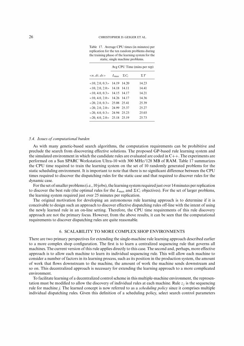
Table 17. Average CPU times (in minutes) perreplication for the ten random problems duringthe training phase of the learning system for the

static, single machine problems.

Avg CPU Time (mins per rep)

<n, dt, ds> Lmax �Ci �T

<10, 2.0, 0.3> 14.19 14.20 14.23

<10, 2.0, 2.0> 14.18 14.11 14.41

<10, 4.0, 0.3> 14.15 14.17 14.21

<10, 4.0, 2.0> 14.26 14.17 14.36

<20, 2.0, 0.3> 25.08 25.41 25.39

<20, 2.0, 2.0> 24.99 25.37 25.27

<20, 4.0, 0.3> 24.94 25.23 25.03

<20, 4.0, 2.0> 25.18 25.19 25.73

5.4. Issues of computational burden

As with many genetic-based search algorithms, the computation requirements can be prohibitive andpreclude the search from discovering effective solutions. The proposed GP-based rule learning system andthe simulated environment in which the candidate rules are evaluated are coded in C++. The experiments areperformed on a Sun SPARC Workstation Ultra-10 with 300 MHz/128 MB of RAM. Table 17 summarizesthe CPU time required to train the learning system on the set of 10 randomly generated problems for thestatic scheduling environment. It is important to note that there is no significant difference between the CPUtimes required to discover the dispatching rules for the static case and that required to discover rules for thedynamic case.

For the set of smaller problems (i.e., 10 jobs), the learning system required just over 14 minutes per replicationto discover the best rule (the optimal rules for the Lmax and �Ci objectives). For the set of larger problems,the learning system required just over 25 minutes per replication.

The original motivation for developing an autonomous rule learning approach is to determine if it isconceivable to design such an approach to discover effective dispatching rules off-line with the intent of usingthe newly learned rule in an on-line setting. Therefore, the CPU time requirements of this rule discoveryapproach are not the primary focus. However, from the above results, it can be seen that the computationalrequirements to discover dispatching rules are quite reasonable.

6. SCALABILITY TO MORE COMPLEX SHOP ENVIRONMENTS

There are two primary perspectives for extending the single-machine rule learning approach described earlierto a more complex shop configuration. The first is to learn a centralized sequencing rule that governs allmachines. The current version of this rule applies directly to this case. The second and, perhaps, more effectiveapproach is to allow each machine to learn its individual sequencing rule. This will allow each machine toconsider a number of factors in its learning process, such as its position in the production system, the amountof work that flows downstream to the machine, the amount of work the machine sends downstream andso on. This decentralized approach is necessary for extending the learning approach to a more complicatedenvironment.

To facilitate learning of a decentralized control scheme in this multiple-machine environment, the represen-tation must be modified to allow the discovery of individual rules at each machine. Rule z j is the sequencingrule for machine j. The learned concept is now referred to as a scheduling policy since it comprises multipleindividual dispatching rules. Given this definition of a scheduling policy, select search control parameters


need to be modified, including the population of scheduling policies and the search operators crossover andmutation.

6.1. Redefinition of a population

The redefinition of a population begins with each machine j possessing a set Zj of s candidate rules. Inother words,

Zj = ]z1

j , . . . , zsj

⌋, (12)

where Z kj is a sequencing rule k in the set of s rules at machine j. Therefore, we define population P as all

instances of rule combinations across the m machines where the population size is sm.

6.2. Modification of search operators

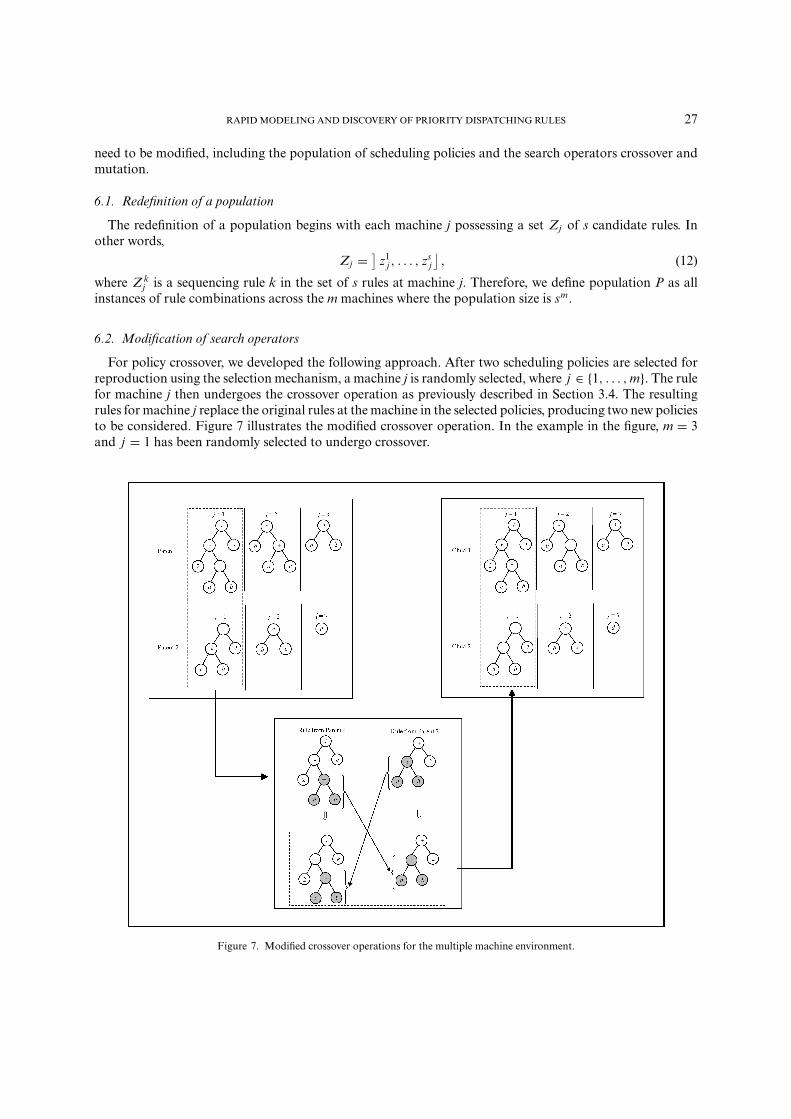
For policy crossover, we developed the following approach. After two scheduling policies are selected forreproduction using the selection mechanism, a machine j is randomly selected, where j ∈ {1, . . . , m}. The rulefor machine j then undergoes the crossover operation as previously described in Section 3.4. The resultingrules for machine j replace the original rules at the machine in the selected policies, producing two new policiesto be considered. Figure 7 illustrates the modified crossover operation. In the example in the figure, m = 3and j = 1 has been randomly selected to undergo crossover.

Figure 7. Modified crossover operations for the multiple machine environment.


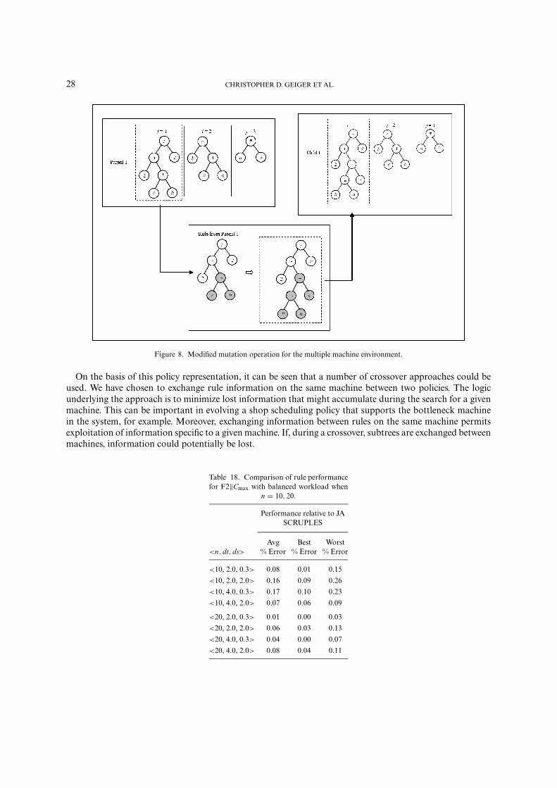
Figure 8. Modified mutation operation for the multiple machine environment.

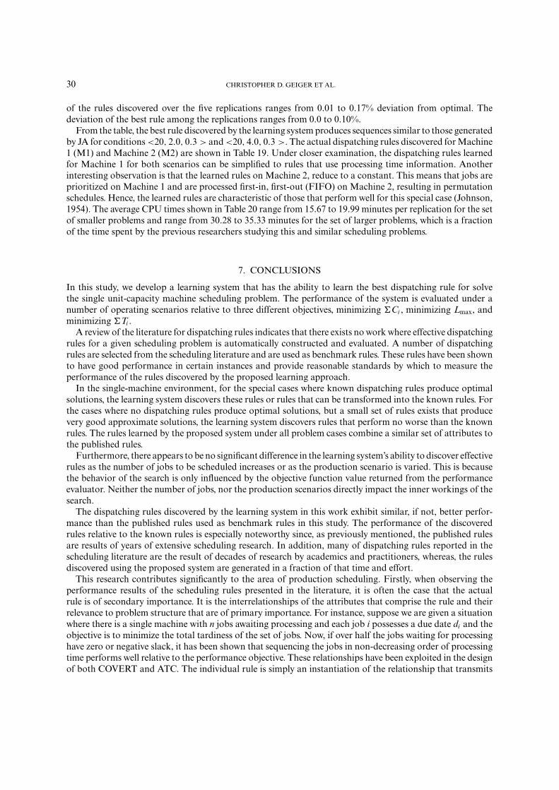
On the basis of this policy representation, it can be seen that a number of crossover approaches could beused. We have chosen to exchange rule information on the same machine between two policies. The logicunderlying the approach is to minimize lost information that might accumulate during the search for a givenmachine. This can be important in evolving a shop scheduling policy that supports the bottleneck machinein the system, for example. Moreover, exchanging information between rules on the same machine permitsexploitation of information specific to a given machine. If, during a crossover, subtrees are exchanged betweenmachines, information could potentially be lost.

Table 18. Comparison of rule performancefor F2‖Cmax with balanced workload when

n = 10, 20.

Performance relative to JASCRUPLES

Avg Best Worst<n, dt, ds> % Error % Error % Error

<10, 2.0, 0.3> 0.08 0.01 0.15

<10, 2.0, 2.0> 0.16 0.09 0.26

<10, 4.0, 0.3> 0.17 0.10 0.23

<10, 4.0, 2.0> 0.07 0.06 0.09

<20, 2.0, 0.3> 0.01 0.00 0.03

<20, 2.0, 2.0> 0.06 0.03 0.13

<20, 4.0, 0.3> 0.04 0.00 0.07

<20, 4.0, 2.0> 0.08 0.04 0.11


As in the crossover operation, for policy mutation, a scheduling policy is selected for reproduction. Then,a machine j ∈ {1, . . . , m} is randomly selected. The rule for machine j then undergoes the mutation opera-tion described in Section 3.4. Figure 8 illustrates the modified mutation operation that is performed on thescheduling policy representation where m = 3 and j = 1 has been randomly selected to undergo mutation.

6.3. An illustration—A balanced two-machine flowshop

The performance of the learning system is analyzed by examining a balanced two-machine flowshop, wherethe average job-processing times on both machines are equal. Examination of the performance of our learningapproach is restricted to a static environment where minimizing makespan (Cmax) is the objective. Johnson(1954) developed a polynomial time algorithm that solves the static two-machine flowshop scheduling problemminimizing makespan (F2||Cmax) optimally. Johnson’s Algorithm (JA) is used as the benchmark rule for thisproblem. Additionally, a set of terminals, similar to those for Machine 1 in Appendix B, are made availableto the learning system for Machine 2.

6.4. Discussion of results for the static, balanced two-machine flowshop

The best-learned policies are quite competitive with JA, in many cases generating similar job sequences.Table 18 summarizes the performance of the learned rules relative to JA and F2||Cmax. The average performance

Table 19. Actual learned policies for F2‖Cmax for <20, 2.0, 0.3 > and <20, 4.0, 0.3 >.

Learned Policy

<n, dt, ds> Machine 1 Rule Machine 2 Rule

<20, 2.0, 0.3> (ADD (EXP (SUB minproctime 1 (POW (EXP (POW(SUB proctime 2 avgqueuetime 1sumqueuetime 1))) proctime 1) avgqueuetime 1)) queuetime)

<20, 4.0, 0.3> (ADD (NEG proctime 2) (MAX (IFLTE minproctime all (EXPmaxduedate 2 (MAX currenttime 10) avgproctime 2remproctime))) sumproctime 2)

Table 20. Average CPU times(in minutes) per replication forthe ten random problems dur-ing the training phase of thelearning system for the static,balanced two-machine flowshop

problem minimizing Cmax.

Avg CPU Time<n, dt, ds> (mins per rep)

<10,2.0,0.3> 15.67

<10, 2.0, 2.0> 17.31

<10,4.0, 0.3> 16.80

<10, 4.0,2.0> 19.99

<20, 2.0, 0.3> 35.33

<20, 2.0, 2.0> 30.28

<20, 4.0, 0.3> 32.68

<20, 4.0, 2.0> 34.18


of the rules discovered over the five replications ranges from 0.01 to 0.17% deviation from optimal. Thedeviation of the best rule among the replications ranges from 0.0 to 0.10%.

From the table, the best rule discovered by the learning system produces sequences similar to those generatedby JA for conditions <20, 2.0, 0.3 > and <20, 4.0, 0.3 >. The actual dispatching rules discovered for Machine1 (M1) and Machine 2 (M2) are shown in Table 19. Under closer examination, the dispatching rules learnedfor Machine 1 for both scenarios can be simplified to rules that use processing time information. Anotherinteresting observation is that the learned rules on Machine 2, reduce to a constant. This means that jobs areprioritized on Machine 1 and are processed first-in, first-out (FIFO) on Machine 2, resulting in permutationschedules. Hence, the learned rules are characteristic of those that perform well for this special case (Johnson,1954). The average CPU times shown in Table 20 range from 15.67 to 19.99 minutes per replication for the setof smaller problems and range from 30.28 to 35.33 minutes for the set of larger problems, which is a fractionof the time spent by the previous researchers studying this and similar scheduling problems.

7. CONCLUSIONS

In this study, we develop a learning system that has the ability to learn the best dispatching rule for solvethe single unit-capacity machine scheduling problem. The performance of the system is evaluated under anumber of operating scenarios relative to three different objectives, minimizing �Ci , minimizing Lmax, andminimizing �Ti .

A review of the literature for dispatching rules indicates that there exists no work where effective dispatchingrules for a given scheduling problem is automatically constructed and evaluated. A number of dispatchingrules are selected from the scheduling literature and are used as benchmark rules. These rules have been shownto have good performance in certain instances and provide reasonable standards by which to measure theperformance of the rules discovered by the proposed learning approach.

In the single-machine environment, for the special cases where known dispatching rules produce optimalsolutions, the learning system discovers these rules or rules that can be transformed into the known rules. Forthe cases where no dispatching rules produce optimal solutions, but a small set of rules exists that producevery good approximate solutions, the learning system discovers rules that perform no worse than the knownrules. The rules learned by the proposed system under all problem cases combine a similar set of attributes tothe published rules.

Furthermore, there appears to be no significant difference in the learning system’s ability to discover effectiverules as the number of jobs to be scheduled increases or as the production scenario is varied. This is becausethe behavior of the search is only influenced by the objective function value returned from the performanceevaluator. Neither the number of jobs, nor the production scenarios directly impact the inner workings of thesearch.

The dispatching rules discovered by the learning system in this work exhibit similar, if not, better perfor-mance than the published rules used as benchmark rules in this study. The performance of the discoveredrules relative to the known rules is especially noteworthy since, as previously mentioned, the published rulesare results of years of extensive scheduling research. In addition, many of dispatching rules reported in thescheduling literature are the result of decades of research by academics and practitioners, whereas, the rulesdiscovered using the proposed system are generated in a fraction of that time and effort.

This research contributes significantly to the area of production scheduling. Firstly, when observing theperformance results of the scheduling rules presented in the literature, it is often the case that the actualrule is of secondary importance. It is the interrelationships of the attributes that comprise the rule and theirrelevance to problem structure that are of primary importance. For instance, suppose we are given a situationwhere there is a single machine with n jobs awaiting processing and each job i possesses a due date di and theobjective is to minimize the total tardiness of the set of jobs. Now, if over half the jobs waiting for processinghave zero or negative slack, it has been shown that sequencing the jobs in non-decreasing order of processingtime performs well relative to the performance objective. These relationships have been exploited in the designof both COVERT and ATC. The individual rule is simply an instantiation of the relationship that transmits


the relationship to the problem environment. This is a simple example; however, it illustrates that, by knowingthe interrelationships among a set of system attributes (in this case, job slack, job processing time and theperformance objective total tardiness), a user is equipped to design an effective scheduling rule if they considermeaningful relationships among the set of system attributes.

Secondly, the development of a learning algorithm that constructs scheduling rules will be a valuableassistant to practitioners as well as provide useful insights to researchers. The method of rule discoverywe use here will identify a rule that performs best under the shop conditions of interest. This resultingscheduling rule may resemble an existing rule in the scheduling literature or may result in a new rule not yetdiscovered.

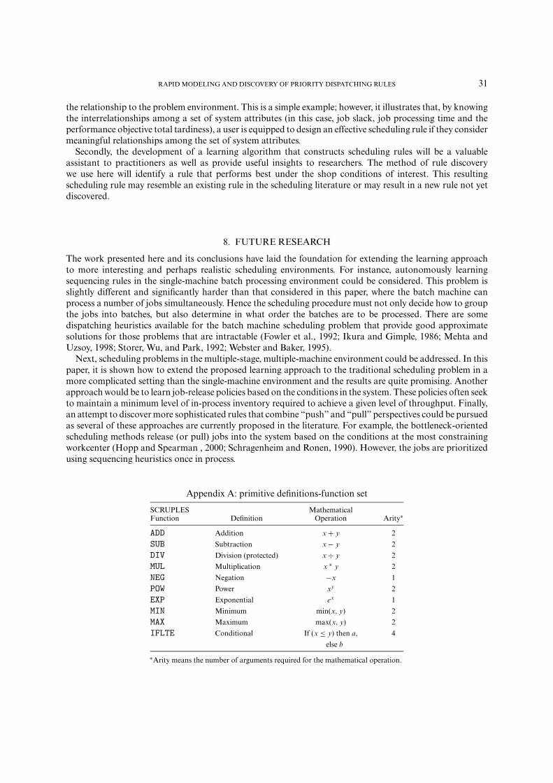
8. FUTURE RESEARCH

The work presented here and its conclusions have laid the foundation for extending the learning approachto more interesting and perhaps realistic scheduling environments. For instance, autonomously learningsequencing rules in the single-machine batch processing environment could be considered. This problem isslightly different and significantly harder than that considered in this paper, where the batch machine canprocess a number of jobs simultaneously. Hence the scheduling procedure must not only decide how to groupthe jobs into batches, but also determine in what order the batches are to be processed. There are somedispatching heuristics available for the batch machine scheduling problem that provide good approximatesolutions for those problems that are intractable (Fowler et al., 1992; Ikura and Gimple, 1986; Mehta andUzsoy, 1998; Storer, Wu, and Park, 1992; Webster and Baker, 1995).

Next, scheduling problems in the multiple-stage, multiple-machine environment could be addressed. In thispaper, it is shown how to extend the proposed learning approach to the traditional scheduling problem in amore complicated setting than the single-machine environment and the results are quite promising. Anotherapproach would be to learn job-release policies based on the conditions in the system. These policies often seekto maintain a minimum level of in-process inventory required to achieve a given level of throughput. Finally,an attempt to discover more sophisticated rules that combine “push” and “pull” perspectives could be pursuedas several of these approaches are currently proposed in the literature. For example, the bottleneck-orientedscheduling methods release (or pull) jobs into the system based on the conditions at the most constrainingworkcenter (Hopp and Spearman , 2000; Schragenheim and Ronen, 1990). However, the jobs are prioritizedusing sequencing heuristics once in process.

Appendix A: primitive definitions-function set

SCRUPLES MathematicalFunction Definition Operation Arity∗

ADD Addition x + y 2

SUB Subtraction x − y 2

DIV Division (protected) x ÷ y 2

MUL Multiplication x ∗ y 2

NEG Negation −x 1

POW Power xy 2

EXP Exponential ex 1

MIN Minimum min(x, y) 2

MAX Maximum max(x, y) 2

IFLTE Conditional If (x ≤ y) then a, 4

else b

∗Arity means the number of arguments required for the mathematical operation.


Appendix B: Primitive Definitions—Terminal Set

Attribute SCRUPLESType Terminal Definition

System currenttime Current timeMachine sumjobs 1 Total number of jobs in queue at Machine 1

sumproctime 1 Total job processing time at Machine 1avgproctime 1 Average job processing time at Machine 1minproctime 1 Minimum job processing time at Machine 1maxproctime 1 Maximum job processing time at Machine 1sumqueuetime 1 Total job queue time at Machine 1avgqueuetime 1 Average job queue time at Machine 1minqueuetime 1 Minimum job queue time at Machine 1maxqueuetime 1 Maximum job queue time at Machine 1minduedate 1 Minimum job due date at Machine 1maxduedate 1 Maximum job due date at Machine 1

Job releasetime Job release time to the shopproctime 1 Job processing time at Machine 1remproctime Job remaining processing timeduedate Job due datequeuetime Job queue timeslack Job slack

General {0,. . . ,10} Integer constants

ACKNOWLEDGMENTS

The authors would like to thank Karl G. Kempf of Intel Corporation for the idea on which this research isbased. The authors would also like to thank the anonymous reviewer of this paper for their thoroughnessand constructive suggestions. This research was supported by the Naval Research Laboratory and the PurdueResearch Foundation.

REFERENCES

Aho, A. V., R. Sethi, and J. D. Ullman, Compilers: Principles, Techniques and Tools, Addison-Wesley Publishing Company, Reading, MA(1986).

AutoSimulations, Inc., AutoSched AP User’s Manual (1998).Avramidis, A. N., K. J. Healy, and R. Uzsoy, “Control of a batch-processing machine: A computational approach,” International Journal

of Production Research, 36, 3167–3181 (1998).Back, T. and H.-P. Schwefel, “An overview of evolutionary algorithms for parameter optimization,” Evolutionary Computation, 1, 1–23

(1993).Back, T. and H.-P. Schwefel, “Evolutionary computation: An overview,” Proceedings of the IEEE Conference on Evolutionary Computation,

20–29 (1996).Back, T., F. Hoffmeister, and H.-P. Schwefel, “A survey of evolution strategies,” in Belew, R. K. (ed.), Proceedings of the Fourth International

Conference on Genetic Algorithms, Morgan Kaufman, San Mateo, CA, 1991.Bagchi, T. P., Multiobjective Scheduling by Genetic Algorithms, Kluwer Academic Publishers, Boston, MA (1991).Baker, K. R. and J. W. M. Bertrand, “A dynamic priority rule for scheduling against due dates,” Journal of Operations Management, 3,

37–42 (1982).Banzhaf, W., P. Nordin, R. E. Keller, and F. D. Francone, Genetic Programming: An Introduction on the Automatic Evolution of Computer

Programs and Its Applications, Morgan Kaufman, San Francisco, CA, 1998.Bhaskaran, K. and M. Pinedo, Dispatching, in Salvendy, G. (ed.), Handbook of Industrial Engineering, John Wiley and Sons, New York,

NY, 1992 pp. 2184–2198.Blackstone, J. H., D. T. Phillips, and G. L. Hogg, “A state-of-the-art survey of dispatching rules for manufacturing job shop operations,”

International Journal of Production Research, 20, 27–45 (1982).Blazewicz, J., K. H. Ecker, E. Pesch, G. Schmidt, and J. Weglarz, Scheduling Computer and Manufacturing Processes, Springer-Verlag,

Heidelberg, Germany, 1996.Carlier, J. and E. Pinson, “An algorithm for solving the job-shop problem,” Management Science, 35, 164–176 (1988).Chang, Y.-L., T. Sueyoshi, and R. S. Sullivan, “Ranking dispatching rules by data envelopment analysis in a job shop environment,” IIE

Transactions, 28, 631–642 (1996).


Cheng, R., M. Gen, and Y. Tsujimura, “A tutorial survey of job-shop scheduling problems using genetic algorithms: Part II. Hybridgenetic search strategies,” Computers and Industrial Engineering, 39, 51–55 (1999).

Chiu, C. and Y. Yih, “A learning-based methodology for dynamic scheduling in distributed manufacturing systems,” International Journalof Production Research, 33, 3217–3232 (1995).

Cramer, N. L., “A representation for the adaptive generation of simple sequential programs,” in Grefenstette, J.J., ed., Proceedings of theFirst International Conference on Genetic Algorithms and Their Applications, 183–187, Lawrence Erlbaum Associates, Hillsdale, NJ(1985).

Davis, L., (ed.), Handbook on Genetic Algorithms, Van Nostrand Reinhold, New York, NY, 1991.De Jong, K. A., “On Using genetic algorithms to search program spaces,” in J. J. Grefenstette (ed.), Proceedings of the Second International

Conference on Genetic Algorithms and Their Applications, Lawrence Erlbaum Associates, Hillsdale, NJ, pp. 1987).De Jong, K. A., “Learning with genetic algorithms: An overview,” Machine Learning, 3, 121–138 (1988).Della Croce, F., R. Tadei, and G. Volta, “A genetic algorithm for the job shop scheduling problem,” Computers and Operations Research,

22, 15–24 (1995).Dimopoulos, C. and A. M. S. Zalzala, “Genetic programming heuristic for the one-machine total tardiness problem,” in Proceedings of

the 1999 Congress on Evolutionary Computation (CEC ’99), 1999 pp. 2207–2214.Dorndorf, U. and E. Pesch, “Evolution based learning in a job shop scheduling environment,” Computers and Operations Research, 22,

25–40 (1995).ElMaraghy, H., V. Patel, and I. Ben Abdallah, “Scheduling of manufacturing systems under dual-resource constraints using genetic

algorithms,” Journal of Manufacturing Systems, 19, 186–201 (2000).Fowler, J. W., D. T. Phillips, and G. L. Hogg, “Real-Time control of multiproduct bulk–service semiconductor manufacturing processes,”

IEEE Transactions on Semiconductor Manufacturing, 5, 158–163 (1992).Gere, Jr., W. S., “Heuristics in job shop scheduling,” Management Science, 13, 167–190 (1966).Goldberg, D. E., Genetic Algorithms in Search, Optimization, and Machine Learning, Addison-Wesley, Reading, MA,

1989.Grefenstette, J. J., “Optimization of control parameters for genetic algorithms,” IEEE Transactions on Systems, Man and Cybernetics,

16, 122–128 (1986).Haupt, R., “A survey of priority rule-based scheduling,” OR Spektrum, 11, 3–16 (1989).Holland, J. H., Adaptation in Natural and Artificial Systems, University of Michigan Press, Ann Arbor, MI, 1975.Holland, J. H., “Escaping brittleness: The possibilities of general-purpose learning algorithms applied to parallel rule–based systems,”

Machine Learning: An Artificial Intelligence Approach, 2, 48–78 (1986).Holland, J. H. and J. S. Reitman, “Cognitive systems based on adaptive algorithms,” in Waterman, D.A. and Hayes-Roth, F. (eds.),

Pattern-Directed Inference Systems, Academic Press, New York, NY, 1978, 313–329.Hopp, W. J. and M. L. Spearman, Factory Physics, 2nd Ed., McGraw-Hill, New York, NY (2000).Ikura, Y. and M. Gimple, “Scheduling algorithms for a single batch processing machine,” Operations Research Letters, 5, 61–65 (1986).Jackson, J. R., Scheduling a Production Line to Minimize Maximum Tardiness, Research Report 43, Management Science Research

Project, University of California at Los Angeles, Los Angeles, CA (1955).Johnson, S. M., “Optimal two- and three-stage production schedules with setup times included,” Naval Research Logistics Quarterly, 1,

61–68, (1954).Kelton, W. D., R. P. Sadowski, and D. A. Sadowski, Simulation with Arena, 2nd Ed., McGraw Hill, New York, NY, 2001.Khuri, S., T. Back, and J Heitkotter, “An evolutionary approach to combinatorial optimization problems,” in Proceedings of the 22nd

Annual ACM Computer Science Conference, (1994).Koza, J. R., “Hierarchical genetic algorithms operating on populations of computer programs,” in Proceedings of the 11th International

Joint Conference on Artificial Intelligence, 1, Morgan Kaufman, San Mateo, CA, 1989, pp. 768–774.Koza, J. R., Genetic Programming: On the Programming of Computers by Means of Natural Selection, MIT Press, Cambridge, MA, 1992.Lee, C.-Y., S. Piramuthu, and Y.-K. Tsai, “Job shop scheduling with a genetic algorithm and machine learning,” International Journal of

Production Research, 35, 1171–1191 (1997).Mattfeld, D. C., Evolutionary Search and the Job Shop: Investigations on Genetic Algorithms for Production Scheduling, Physica-Verlag,

Heidelberg, Germany, 1996.Mehta, S. V. and R. Uzsoy, “Minimizing total tardiness on a batch processing machine with incompatible job families,” IIE Transactions,

30, 165–178 (1998).Michalewicz, Z. and D. Fogel, How to Solve It: Modern Heuristics, Springer-Verlag, Germany, 2000.Morton, T. E. and D. W. Pentico, Heuristic Scheduling Systems, John Wiley and Sons, New York, NY, 1993.Norman, B. and J. Bean, “A genetic algorithm methodology for complex scheduling problems,” Naval Research Logistics, 46, 199–211,

(1999).Norman, B. and J. Bean, “Random keys genetic algorithm for job shop scheduling,” Engineering Design and Automation, 3,145–156,

(1997).Olafsson, S., “Data mining for production scheduling,” in Proceedings of the Industrial Engineering Research Conference (IERC’03),

CD-ROM, (2003).Ovacik, I. M. and R. M. Uzsoy, “Exploiting shop floor status information to schedule complex job shops,” Journal of Manufacturing

Systems, 13, 73–84 (1994).


Ovacik, I. M. and R. Uzsoy, Decomposition Methods for Complex Factory Scheduling Problems, Kluwer Academic Publishers, Boston,MA (1997).

Panwalkar, S. S. and W. Iskander, “A survey of scheduling rules,” Operations Research, 25, 45–61, 1977.Pierreval, H. and N. Mebarki, “dynamic selection of dispatching rules for manufacturing system scheduling,” International Journal of

Production Research, 35, 1575–1591, 1997.Pinedo, M., Scheduling: Theory, Algorithms and Systems, Prentice Hall, Englewood Cliffs, NJ (2002).Piramuthu, S., N. Raman, and M. J. Shaw, “Learning-based scheduling in a flexible manufacturing flow line,” IEEE Transactions on

Engineering Management, 41, 172–182, 1994.Pritsker, A. A. B., J. J. O’Reilly, and D. K LaVal, Simulation with Visual SLAM and Awesim, John Wiley and Sons, New York, NY, 1997.Reeves, C. R. (ed.), Modern Heuristic Techniques for Combinatorial Problems, John Wiley and Sons, New York, NY, 1993.Russell, R. S., E. M. Dar-El, and B. W. Taylor, III, “A comparative analysis of the covert job sequencing rule using various shop

performance measures,” International Journal of Production Research, 25, 1523–1540 (1987)Russell, S. J. and P. Norvig, Artificial Intelligence: A Modern Approach, Prentice Hall, Upper Saddle River, NJ(1995).Schragenheim, E. and B. Ronen, “Drum-buffer-rope shop floor control,” Production and Inventory Management, 31, 18–23 (1990).Shaw, M. J., S. Park, and N. Raman, “Intelligent scheduling with machine learning capabilities: The induction of scheduling knowledge,”

IIE Transactions, 24, 156–168 (1992).Smith, W. E., “Various optimizers for single-stage production,” Naval Research Logistics Quarterly, 3, 59–66 (1956).Storer, R. H., S. D. Wu, and I. Park, “Genetic algorithms in problem space for sequencing problems,” in Proceedings of a Joint US-German

Conference on Operations Research in Production Planning and Control, 584–597, (1992).Storer, R. H., S. D. Wu, and R. Vaccari, “New search spaces for sequencing problems with application to job shop scheduling,”

Management Science, 38, 1495–1509, (1992).Uzsoy, R., “Scheduling batch processing machines with incompatible job families,” International Journal of Production Research, 33,

2685–2708 (1995).Vepsalainen, A. P. J. and T. E. Morton, “Priority rules for job shops with weighted tardiness costs,” Management Science, 33, 1035–1047

(1987).Webster, S. and K. R. Baker, “Scheduling groups of jobs on a single machine,” Operations Research, 43, 692–703 (1995).

rapid modeling and discovery of priority dispatching rules

Documents

Transcript of rapid modeling and discovery of priority dispatching rules