DIRECTION OF ARRIVAL ESTIMATION BY ARRAY ...DIRECTION OF ARRIVAL ESTIMATION BY ARRAY INTERPOLATION...

DIRECTION OF ARRIVAL ESTIMATION BY

ARRAY INTERPOLATION IN RANDOMLY

DISTRIBUTED SENSOR ARRAYS

a thesis submitted to

the graduate school of natural and applied sciences

of

the middle east technical university

by

isin akyildiz

in partial fulfillment of the requirements

for

the degree of master of science

in

electrical and electronics engineering

december 2006

Approval of the Graduate School of Natural and Applied Sciences

Prof. Dr. Canan OZGEN

Director

I certify that this thesis satisfies all the requirements as a thesis for the degree

of Master of Science.

Prof. Dr. Ismet ERKMEN

Head of Department

This is to certify that we have read this thesis and that in our opinion it is

fully adequate, in scope and quality, as a thesis for the degree of Master of

Science.

Assoc. Prof. Dr. Engin TUNCER

Supervisor

Examining Committee Members

Prof. Dr. Kemal LEBLEBICIOGLU (METU, EEE)

Assoc. Prof. Dr. Engin TUNCER (METU, EEE)

Assoc. Prof. Dr. Gozde BOZDAGI (METU, EEE)

Asst. Prof. Dr. Afsar SARANLI (METU, EEE)

M. Sc. Aykut ARIKAN (ASELSAN)

I hearby declare that all information in this document has been

obtained and presented in accordance with academic rules and eth-

ical conduct. I also declare that, as required, I have fully cited and

referenced all material and results that are not original to this

work.

Name Lastname : Isın

AKYILDIZ

Signature :

iii

abstract

direction of arrivalestimation by array

interpolation in randomlydistributed sensor arrays

AKYILDIZ, Isın

M.Sc., Department of Electrical and Electronics Engineering

Supervisor: Assoc. Prof. Dr. Engin TUNCER

December 2006, 78 pages

In this thesis, DOA estimation using array interpolation in randomly dis-

tributed sensor arrays is considered. Array interpolation is a technique in

which a virtual array is obtained from the real array and the outputs of the

virtual array, computed from the real array using a linear transformation,

is used for direction of arrival estimation. The idea of array interpolation

technique is to make simplified and computationally less demanding high

resolution direction finding methods applicable to the general class of non-

structured arrays. In this study, two different interpolation technique is

applied for arbitrary array geometries in an attempt to extend root-MUSIC

algorithm to arbitrary array geometries. Another issue of array interpolation

related to direction finding is spatial smoothing in the presence of multipath

sources. It is shown that due to the Vandermonde structure of virtual array

manifold vector obtained from the proposed interpolation methods, it is pos-

iv

sible to use spatial smoothing algorithms for the case of multipath sources.

Keywords: Direction of Arrival Estimation, Root-MUSIC, Randomly Dis-

tributed, Array Interpolation, Spatial Smoothing

v

oz

DUZENSIZ DIZILERDE DIZIARADEGERLENDIRME ILE GELIS ACISI

TAHMINI

AKYILDIZ, Isın

Yuksek Lisans, Elektrik ve Elektronik Muhendisligi Bolumu

Tez Yoneticisi: Doc. Dr. Engin TUNCER

Aralık 2006, 78 sayfa

Duzensiz dizilerde dizi aradegerlendirme ile gelis acısı tahmini ele alınmıstır.

Dizi aradegerlendirme tekniginde, gercek dizi kullanılarak sanal dizi elde

edilir ve sanal dizinin alıcı cıktıları gelis acısı tahmini icin kullanılır. Dizi

aradegerlendirmenin ana amacı basitlestirilmis ve islemsel olarak daha az

kompleks olan yuksek cozunurluklu gelis acısı tahmin metodlarını genel duzenli

yapısı olmayan dizilere de uygulanabilir hale getirmektir. Bu calısmada

duzensiz yerlestirilmis bir alıcı dizini uzerinde aradegerlendirme yapılmıs ve

kok MUSIC algoritması kullanılarak gelis acısı tahmin performansı degerlendi-

rilmistir. Acı aradegerlendirme tekniginin diger bir avantajıda cok yonlu

enerji kaynakları durumunda uzaysal yumusatma algoritmalarının kullanıla-

bilirligidir. Sanal dizi cıktı (manifold) vektorunun ozel Vandermonde yapısı

sebebiyle uzaysal yumusatma metodlarının kullanılabilirligi uzerinde durul-

mustur.

Anahtar sozcukler: Gelis Acısı Tahmini, Duzensiz Diziler, Dizi Aradeger-

vi

lendirmesi, Kok MUSIC, uzaysal yumusatma

vii

to my family and Alper

viii

acknowledgments

I would like to express my sincere gratitude to my supervisor Doc. Dr.

Temel Engin Tuncer for his supervision, guidance and encouragement through-

out this study.

Special thanks to my beloved Alper for his help during the preparation

of the thesis and his great encouragement during this period. Also special

thanks to my friend Kaya for his great support and assistance during the

preperation of the thesis. I would like to deeply thank to my friend Zeynep,

for her drawings in the thesis.

I am forever indepted to my family who have been supporting me in every

aspect of my life.

I would like to express my appreciation to my colleagues for their valuable

support.

ix

table of contents

plagiarism . . . . . . . . . . . . . . . . . . . . . . . . . . . . . . . . . . . . . . . . . . . . . . iii

abstract . . . . . . . . . . . . . . . . . . . . . . . . . . . . . . . . . . . . . . . . . . . . . . . iv

oz . . . . . . . . . . . . . . . . . . . . . . . . . . . . . . . . . . . . . . . . . . . . . . . . . . . . . . . vi

acknowledgements . . . . . . . . . . . . . . . . . . . . . . . . . . . . . . . . . . . ix

table of contents . . . . . . . . . . . . . . . . . . . . . . . . . . . . . . . . . . . . x

chapter

1 Introduction . . . . . . . . . . . . . . . . . . . . . . . . . . . . . . . . . . . . . . . 1

2 Preliminaries . . . . . . . . . . . . . . . . . . . . . . . . . . . . . . . . . . . . . . . 9

2.1 Source . . . . . . . . . . . . . . . . . . . . . . . . . . . . . . . 9

2.2 Sensor Array . . . . . . . . . . . . . . . . . . . . . . . . . . . 10

2.3 Array Response . . . . . . . . . . . . . . . . . . . . . . . . . . 10

2.3.1 The Narrowband Assumption . . . . . . . . . . . . . . 14

2.3.2 The Array Output Model . . . . . . . . . . . . . . . . 15

2.3.3 The Array Output Model: Coherent Sources Case . . . 16

3 a special array geometry: ULA . . . . . . . . . . . . . . . . . 18

3.1 Array Manifold Vector:ULA Case . . . . . . . . . . . . . . . . 19

3.2 The root-MUSIC Algorithm . . . . . . . . . . . . . . . . . . . 22

x

3.3 Spatial Smoothing . . . . . . . . . . . . . . . . . . . . . . . . 24

3.3.1 The Spatial Smoothing Preprocessing Technique . . . . 25

4 array interpolation:virtual array concept . . . 28

4.1 Virtual Array Design For Array Interpolation . . . . . . . . . 28

4.1.1 Problem Formulation . . . . . . . . . . . . . . . . . . . 30

4.1.2 Virtual ULA . . . . . . . . . . . . . . . . . . . . . . . . 30

4.1.3 Direction Finding with Interpolated Array:Virtual ULA

method . . . . . . . . . . . . . . . . . . . . . . . . . . 31

4.1.4 Virtual Array Using Differential Geometry . . . . . . . 32

4.1.5 Arc Length Representation . . . . . . . . . . . . . . . . 33

4.1.6 Direction Finding with Interpolated Array:Virtual Ar-

ray Case . . . . . . . . . . . . . . . . . . . . . . . . . . 38

4.2 Interpolated Spatial Smoothing . . . . . . . . . . . . . . . . . 39

5 Simulation Results . . . . . . . . . . . . . . . . . . . . . . . . . . . . . . . . . 40

5.1 Uncorrelated Sources . . . . . . . . . . . . . . . . . . . . . . . 41

5.1.1 One Source . . . . . . . . . . . . . . . . . . . . . . . . 41

5.1.2 Two Sources . . . . . . . . . . . . . . . . . . . . . . . . 60

5.1.3 Three Sources . . . . . . . . . . . . . . . . . . . . . . . 62

5.2 Interpolated Spatial Smoothing . . . . . . . . . . . . . . . . . 64

5.2.1 Two Sources . . . . . . . . . . . . . . . . . . . . . . . . 64

5.2.2 Three Sources . . . . . . . . . . . . . . . . . . . . . . . 64

5.2.3 Four Sources . . . . . . . . . . . . . . . . . . . . . . . 69

5.3 Virtual Array With Less Array Elements . . . . . . . . . . . . 69

6 conclusion . . . . . . . . . . . . . . . . . . . . . . . . . . . . . . . . . . . . . . . . . . 73

references . . . . . . . . . . . . . . . . . . . . . . . . . . . . . . . . . . . . . . . . . . . . . 74

xi

list of figures

1.1 Airborne RADAR . . . . . . . . . . . . . . . . . . . . . . . . . 2

1.2 Rescue SONAR . . . . . . . . . . . . . . . . . . . . . . . . . . 3

1.3 Towed Array . . . . . . . . . . . . . . . . . . . . . . . . . . . 4

1.4 Geophone Array . . . . . . . . . . . . . . . . . . . . . . . . . . 5

2.1 m-element randomly distributed array . . . . . . . . . . . . . 11

3.1 m-element uniform linear array . . . . . . . . . . . . . . . . . 20

5.1 Real array element positions . . . . . . . . . . . . . . . . . . . 42

5.2 The interpolation sector and real array element positions . . . 43

5.3 Performances of two interpolation methods and comparison

with CRB of the original array when the source DOA angle is

changing from 0o to 180o degrees. (Interpolation sector is [0o

180o] degrees. SNR 60 dB) . . . . . . . . . . . . . . . . . . . . 44




180o] degrees. SNR 30 dB) . . . . . . . . . . . . . . . . . . . . 45




180o] degrees. SNR 10 dB) . . . . . . . . . . . . . . . . . . . . 46

5.6 The interpolation sector and real array element positions . . . 47

xii




72o] degrees. SNR 60 dB) . . . . . . . . . . . . . . . . . . . . 48




72o] degrees. SNR 30 dB) . . . . . . . . . . . . . . . . . . . . 49




72o] degrees. SNR 10 dB) . . . . . . . . . . . . . . . . . . . . 50

5.10 Number of snapshot effect. Source DOA angle is changing

from 88o to 93o degrees. (Interpolation sector is [88o 93o] de-

grees). SNR 30 dB. Number of snapshots 100 . . . . . . . . . 52

5.11 Number of snapshot effect. Source DOA angle is changing

from 88o to 93o degrees. (Interpolation sector is[88o 93o] de-

grees). SNR 30 dB. Number of snapshots 1000 . . . . . . . . . 53

5.12 Frobenius norm ratio versus interpolation sector width . . . . 54

5.13 Interpolation matrix condition number versus interpolation

sector width . . . . . . . . . . . . . . . . . . . . . . . . . . . 55

5.14 Frobenius norm ratio versus interpolation sector partition . . 56

5.15 Interpolation matrix condition number versus interpolation

sector partition . . . . . . . . . . . . . . . . . . . . . . . . . . 57

5.16 Performances of two interpolation methods compared with

CRB for one source with DOA angle 58o. (Interpolation sector

[45o 72o]). . . . . . . . . . . . . . . . . . . . . . . . . . . . . . 58

xiii


CRB for one source with DOA angle 58o. (Interpolation sector

[0o 180o]). . . . . . . . . . . . . . . . . . . . . . . . . . . . . . 59

5.18 The interpolation sector and the sources impinging on the real

array . . . . . . . . . . . . . . . . . . . . . . . . . . . . . . . 60


CRB for two equipower uncorrelated sources with DOA an-

gles 58o and 63o. (Interpolation sector [45o 72o]). . . . . . . . . 61


array . . . . . . . . . . . . . . . . . . . . . . . . . . . . . . . 62


CRB for three equipower uncorrelated sources with DOA an-

gles 58o, 63o and 70o .(Interpolation sector [45o 72o]). . . . . . 63


array . . . . . . . . . . . . . . . . . . . . . . . . . . . . . . . 65


CRB for three equipower sources with DOA angles 58o, 63o

and 70o one of which is coherent with correlation coefficient

α = 0.7391 and β = 0.3061 .(Interpolation sector [45o 72o]). . . 66


array . . . . . . . . . . . . . . . . . . . . . . . . . . . . . . . 67


CRB for three equipower sources with DOA angles 45o, 60o

and 115o two of which are coherent with correlation coefficient

α = 0.4,−0.3 and β = 0.8,−0.7 respectively .(Interpolation

sector [20o 120o]). . . . . . . . . . . . . . . . . . . . . . . . . . 68


array . . . . . . . . . . . . . . . . . . . . . . . . . . . . . . . 70

xiv


CRB for four equipower sources with DOA angles 15o,45o, 60o

and 115o three of which are coherent with correlation coeffi-

cient α = 0.4,−0.3, 0.5 and β = 0.8,−0.7,−0.6 respectively

.(Interpolation sector [0o 120o]). . . . . . . . . . . . . . . . . . 71

5.28 Interpolation quality comparison for 8 element interpolated

array and 13 element interpolated array . . . . . . . . . . . . 72

xv

chapter 1

Introduction

Array signal processing deals with the processing of information bearing

signals collected by an array of sensors operating in a physical environment

of interest in order to execute an estimation task. Identifying the location of

targets or the direction of arrival (DOA) of any signal is one of the defined

estimation tasks. In the DOA estimation problem, the data from the target,

i.e., the source of energy, which may be electromagnetic wave, acoustic wave

or seismic wave, etc, is processed in order to obtain its location or DOA

angle. The sensor array can be passive or active. In a passive system, the

sensor array has the task of listening to the environment. In this case, the

energy source is the target itself. In an active system, on the other hand, a

transmitter emits energy to the environment and the sensor array listens to

the environment for the response of the target. The sensors may have several

forms depending on the type of energy radiated from the target. They may

be antennas as in RADAR, radio communications and radio astronomy, or

hydrophones as in SONAR, or geophones as in seismology, or microphones as

in acoustics, or x-ray detectors as in medical imaging. Independent of their

type, the sensors are designed to provide an interface between the physical

environment in which the array is embedded and signal processing part of

the system. The role of the sensors in an array signal processing system is to

convert the physical energy to the electrical signals and the function of the

processor is to produce the estimates of the target parameters of interest by

using the information contained in the electrical signals. The target param-

1

Figure 1.1: Airborne RADAR

eters of interest may be the shape of the target, the DOA of the target or

the number of sources.

Array signal processing is very important in RADAR, SONAR, seismic

systems, electronic surveillance, medical diagnosis and treatment and radio

astronomy.

In RADAR, antenna array is used for both transmission and reception of

signals. Some military applications of antenna array systems include phased

array RADAR systems which are used for ballistic missile detection.

Antenna arrays are widely used in radio astronomy area. A radio astron-

omy array system is a passive array system which is used for the detection

of celestial objects and the estimation of their characteristics.

Arrays are widely used in SONAR systems. There are two types of

SONAR system which are active and passive SONAR. In active SONAR,

acoustic energy is transmitted in water and the reflections from the target

listened by the array system are processed in order to detect the target. The

theory of active SONAR has very much in common with active RADAR.

2

Figure 1.2: Rescue SONAR

Passive SONAR systems only listen to the water for the acoustic energy

caused by the active target and process the data obtained from the target

in order to locate the target. A good example for hydrophone array system

application is the towed array which is towed from the hull of a ship in order

to listen to the ocean to detect torpedoes. In Figure 1.3 such a towed array

system is shown.

There are two areas of seismology in which array signal processing plays

an important role. First one is the detection and the localization of the un-

derground explosions. The second area is the exploration seismology. In the

exploration seismology, an active source transmits energy to the subsurface

and the seismic array on the surface listens to the echoes and constructs the

image of the subsurface in which the structure and physical properties are

described.

Independent from the type of energy transmitted from the target, the

direction finding (DF) or DOA estimation problem is theoretically defined as

the estimation of the propagation direction of a wave. Due to its widespread

application and difficulty of obtaining optimum estimator, the topic has re-

3

Figure 1.3: Towed Array

ceived a significant amount of attention over the last several decades and

a large quantity of algorithms for different scenarios for a variety of array

structures have been developed.

The DOA estimation techniques can be classified into two main cate-

gories, namely the spectral-based and the parametric approach. In the spec-

tral based approach, a spectrum-like function for DOAs are formed and the

values at which the function in question gives peaks are found as the DOA

estimates. In the parametric approach, the signal waveforms are modeled

as random processes and the DOA estimates are found by minimizing some

statistical functions parameterized by the DOAs. The parametric approach

results in more accurate estimates. However, the parametric techniques are

computationally much more demanding compared to spectral-based tech-

niques. The usage of the parametric techniques is preferable for the case

when coherent sources are involved in the DOA estimation problem. The

spectral-based techniques can also be grouped under two different subclasses,

the beamforming techniques and the subspace-based techniques.

In beamforming techniques, the main idea is to steer the array and mea-

sure the output power. The points at which the output power give peaks are

4

Figure 1.4: Geophone Array

recorded as the DOA estimates. The conventional beamformer, namely the

Bartlett beamformer is introduced by Bartlett in [2] and is a general exten-

sion of the fourier-based spectral analysis. It is further developed by Capon

in [7], in order to improve resolution capability of the beamformer for two

closely spaced sources.

In subspace-based techniques, the eigen-structure of the observed data

covariance matrix is directly used in order to find the DOA estimates. The

first subspace-based algorithm is called MUSIC (Multiple Signal Classifica-

tion), and was introduced by Schmidt in [24], [25], [26] and independently by

Bienvenu and Kopp in [3] and [4]. For standard linear arrays, root-MUSIC

and ESPRIT (Estimation of Signal Parameters via Rotational Invariance) is

introduced in [1], [19] and [22], respectively. The subspace-based algorithms

have an increased resolution compared to beamforming techniques, due to

the fact that no windowing of the data is required.

The spectral-based methods are computationally less demanding than the

parametric methods. However, especially for the scenarios involving highly

5

correlated signals, the performance of spectral-based methods may be insuffi-

cient. The parametric methods yield more accurate solutions. Unfortunately,

these methods require multidimensional search to find the estimates, which

is computationally quite complex. The most well known and frequently used

parametric algorithm is the Maximum Likelihood (ML) technique [28].

Another important classification of the DOA estimation approaches can

be done depending on the array geometry which is required for the technique

used. The array with special arrangement of sensors, especially the uniform

linear array (ULA) gives the opportunity to use high resolution, computa-

tionally less demanding and simplified subspace-based techniques like root-

MUSIC, RARE, IQML, conventional and multiple invariance ESPRIT. All

this algorithms require uniform linear arrays and/or array geometries with

shift-invariances.

Another central problem in the area of the array processing related to

the DOA is the DOA estimation in the case of fully correlated plane waves

or signals. This case referred as the coherent signal case, appears in specular

multipath propagation and has been therefore gained great practical impor-

tance. A preprocessing technique called spatial smoothing for dealing with

coherent signals which allows the use of low-complexity DOA methods for

only ULA is proposed by Evans et al. and Shan et al. in [8] and in [27]

further developed by Pillai in [20].

None of the mentioned algorithms can be utilized for the case of array

geometries different than ULA. In an attempt to exploit these computation-

ally less demanding and simplified high resolution algorithms for the general

class of array geometries, the concept of array interpolation is introduced to

the literature by Friedlander in [10] and [12]. The array interpolation is a

technique in which a virtual array is obtained from the real array and the

outputs of the virtual array, computed from the real array using a linear

transformation, is used for direction of arrival estimation. The interpolated

6

array concept not only broadened the mentioned algorithms to the general

class of array geometries but also have many other advantages, like the ex-

pansion of spatial smoothing preprocessing technique to the randomly dis-

tributed array geometries. The interpolated spatial smoothing technique is

introduced to the literature by Friedlander in [11].

In this work, the DOA estimation problem in randomly distributed sensor

arrays by using two different interpolation methods is considered. The first

method is the array interpolation method with virtual ULA and introduced

by Friedlander in [10]. In the second array interpolation method a virtual

array manifold vector is used for the DOA estimation [6]. As mentioned in the

subsequent paragraph, the aim of the array interpolation is the separation to

some extent the DOA estimation problem from the physical locations of the

array elements. This is done by obtaining a virtual array from the real array

by a linear interpolation technique and the DOA estimation is done by using

outputs from the virtual array elements rather than the real array elements.

The two interpolation methods considered in this work differ in the selection

of virtual array. In the first method, the virtual array is a uniformly spaced

array, the design of which is under the control of the designer with some

restrictions. However, the virtual array is not a physical array in the second

method. It is obtained from the real array manifold vector by using arc

length approximation. The steps involved in the virtual array creation and

interpolation matrix design are considered in detail for the two interpolation

methods. The root-MUSIC algorithm is used for the DOA estimation. The

spatial preprocessing technique is used for the DOA estimation when the

sources are correlated. The interpolated spatial smoothing techniques are

introduced to the literature by Friedlander for virtual ULA in [11]. However,

in this application, the spatial smoothing preprocessing technique is applied

to a non-physical virtual array having the necessary Vandermonde structure.

The work is organized as follows. In Chapter 2, some preliminary knowl-

7

edge on wave equation is given. The array response to an external signal

field is mathematically formulated in order to obtain the stochastic model

used for the DOA estimation with the narrowband assumption on sources.

The array manifold vector concept is introduced. In Chapter 3, the array

manifold vector for ULA is obtained. The Vandermonde structure of array

manifold vector for ULA is emphasized and the formulization of the root-

MUSIC algorithm and the spatial smoothing algorithm for the correlated

sources case are given. In Chapter 4, virtual array concept is introduced.

The two interpolation methods for the interpolation matrix design are ex-

plained in detail. The interpolated root-MUSIC and the interpolated spatial

smoothing algorithms are mathematically formulized. In Chapter 5, the sim-

ulation results for the performance analysis of the interpolated root-MUSIC

with the two interpolation methods and the spatial smoothing preprocessing

are presented. Finally, in Chapter 6, the conclusion is provided.

8

chapter 2

Preliminaries

As stated in the previous chapter, in the DOA estimation problem the

data from the target may be electromagnetic wave, sound wave, or seismic

wave, etc. However, in this thesis the DOA estimation problem for acoustic

sources is investigated. In this chapter, the sound wave equation and its solu-

tion for plane waves with narrowband assumption is given and the response

of a microphone array system to this source is formulized. The array output

data model for the DOA estimation with narrowband assumption on sources

is obtained.

2.1 Source

General equation of a sound wave in three dimensional space is given as

∆2p(ξ, t) =1

c2

∂2p(ξ, t)

∂t2(2.1)

where c is the speed of sound, ξ is the three-dimensional space coordinates

and t is time variable. In the discussion, it is assumed that the sound sources

are in the far-field, i.e., they are far enough so that the solution of wave

equation gives plane waves. For this case, the solution of the wave equation

for planar real sound wave is mathematically expressed as

p(ξ) = P1ej(ω/c)ξ + P2e

−j(ω/c)ξ (2.2)

It is also assumed that the media where the sound waves propagate is homo-

geneous, i.e., the speed of plane waves is independent from the coordinates

9

of the propagation region. The incoming signal is just a complex exponential

at the fixed frequency ω.

2.2 Sensor Array

Microphone sensor arrays have arbitrary geometry and they are posi-

tioned in xy-plane as shown in Figure 2.1. The sensor positions should satisfy

the sampling theorem. This means that the array elements must be less than

a half wavelength apart. The plane wave and the sensor array are assumed

to be on the same plane. Another assumption is that all microphones are

calibrated with the known frequency response and they are isotropic, i.e.,

their response is independent of the DOA of the sources.

2.3 Array Response

The array output model is the central part of DOA estimation problem.

The array response of a microphone array to a plane wave is formulized in

this section. The array consists of isotropic sensors with the known frequency

response. The sensors in Figure 2.1 spatially sample the signal field at the

locations pn:n= 0, 1, . . . , m − 1. This yields a set of signals denoted by−→f (t,−→p )

−→f (t,−→p ) =

f(t, p0)

f(t, p1)...

f(t, pm−1)

(2.3)

Assuming that the impulse response of the nth sensor is hn(t) and nth sensor

output is yn(t), the sensor impulse response vector and the sensor output

10

Figure 2.1: m-element randomly distributed array

11

vector is given as

−→h (T ) =

h0(T )

h1(T )...

hm−1(T ))

and −→y (t) =

y0(t)

y1(t)...

ym−1(t))

(2.4)

yn(t) = hn(t) ∗ f(t− Tn) =

∫ +∞

−∞hn(t− T )f(T, pn)dT (2.5)

Taking the Fourier Transform of both sides and expressing the equation in

the Fourier domain yields

Yn(w) = Hn(w)F (w, pn) (2.6)

where the input is assumed to be a plane wave propagating in the direction

a with center (frequency f) radian frequency w and c is the speed of the

propagation in the air (or in the medium). If f(t) is the signal received at

the origin of the coordinate system (or the center of gravity of sensors), then

the signals impinging on the sensors are the delayed versions of f(t). The

vector of arriving signals can be written as

−→f (t,−→p ) =

f(t− T0)

f(t− T1)...

f(t− Tm−1)

where Tn =aT pn

cand a =

(−cos(θ)

−sin(θ)

)

(2.7)

where Tn is the time delay corresponding to the time of arrival at the nth

sensor and Tn is given as

Tn =−xncos(θ)− ynsin(θ)

cwhere pn =

(xn

yn

)(2.8)

12

Expressing sensor output equation (2.5) in Fourier Domain yields

Yn(w) = Hn(w)F (w, pn) = Hn(w)e−jwTnF (w) = Hn(w)ejw(xncos(θ)+ynsin(θ))

c F (w)

(2.9)

For a plane wave propagating in the direction a with the radian frequency w

with propagation speed c the wavenumber vector is defined as

−→k = −→a 2π

λand k = ‖−→k ‖ =

2π

λ(2.10)

Then the above equation can be written as

Yn(w) = Hn(w)ej2π(xncos(θ)+ynsin(θ))

λ F (w) (2.11)

If the sensor coordinates are given in terms of wavelength, then (2.11) can

be rewritten as

Yn(w) = Hn(w)ej2π(xncos(θ)+ynsin(θ))F (w) (2.12)

Assuming that all the sensors are identical and their frequency response at

w is the same and H(w), then the sensor output vector can be expressed as

−→Y (w) = H(w)F (w)

ej2π(x0cos(θ)+y0sin(θ))



...

ej2π(xm−1cos(θ)+ym−1sin(θ))

(2.13)

The matrix in (2.14) is called as the Array Manifold Vector

a(θ) =




...


(2.14)

13

Since it is assumed that f(t) is a plane wave propagating in the direction a

with radian frequency w with the propagation speed c, the equation in (2.13)

also holds in time domain, i.e.,

−→y (t) = H(w)f(t)




...


(2.15)

In the classical array theory the output for a plane wave propogating in

the direction a with radian frequency w with the propagation speed c, the

output at each sensor is given by (2.15) .

For obtaining the output sensor equation in time domain, the main as-

sumption is that our plane waves are propagating at single frequency. In

the next subsection, it is shown that when the waves are narrowband, then

the same equation still holds. The assumption is called as the narrowband

assumption.

2.3.1 The Narrowband Assumption

The sensor output equation is obtained for the case when the plane waves

are bandpass signals. In this case, the signal at a location pn is expressed as

f(t, pn) =√

2Re{f(t, pn)ejwct} where n = 0, 1, . . . , m− 1 (2.16)

where wc is the carrier frequency and f(t, pn) is the complex envelope. As-

suming that the complex envelope is band-limited to the region

wl ≤ 2πB/2 (2.17)

14

f(t, pn) =√

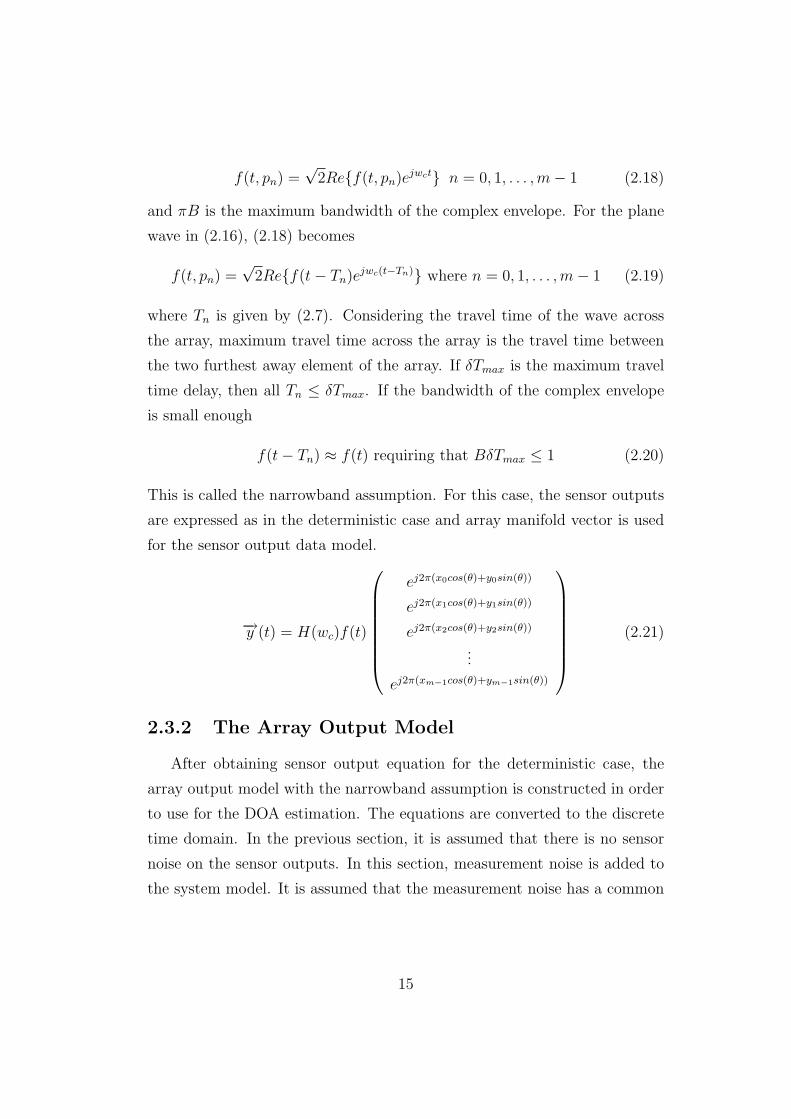
2Re{f(t, pn)ejwct} n = 0, 1, . . . , m− 1 (2.18)

and πB is the maximum bandwidth of the complex envelope. For the plane

wave in (2.16), (2.18) becomes

f(t, pn) =√

2Re{f(t− Tn)ejwc(t−Tn)} where n = 0, 1, . . . , m− 1 (2.19)

where Tn is given by (2.7). Considering the travel time of the wave across

the array, maximum travel time across the array is the travel time between

the two furthest away element of the array. If δTmax is the maximum travel

time delay, then all Tn ≤ δTmax. If the bandwidth of the complex envelope

is small enough

f(t− Tn) ≈ f(t) requiring that BδTmax ≤ 1 (2.20)

This is called the narrowband assumption. For this case, the sensor outputs

are expressed as in the deterministic case and array manifold vector is used

for the sensor output data model.

−→y (t) = H(wc)f(t)




...


(2.21)

2.3.2 The Array Output Model

After obtaining sensor output equation for the deterministic case, the

array output model with the narrowband assumption is constructed in order

to use for the DOA estimation. The equations are converted to the discrete

time domain. In the previous section, it is assumed that there is no sensor

noise on the sensor outputs. In this section, measurement noise is added to

the system model. It is assumed that the measurement noise has a common

15

variance σn2 at all sensors and uncorrelated among all the sensors. Such

noise is termed as spatially white and it is a reasonable model for a receiver

noise.

Let an array of m sensors receive n narrowband plane waves from far-field

emitters with the same center frequency fc. The signal model is

x(t) = A(θ)s(t) + n(t) (2.22)

where

A(θ) =(

a(θ1) + αa(θ2) a(θ3) . . . a(θn))T

(2.23)

s(t) is a vector containing the complex signal envelopes of n narrowband

signal sources located in the xy plane, n(t) is mX1 vector of zero mean

spatially white sensor noise of variance σn2 and the columns of the array

manifold matrix or the array steering matrix A(θ) are the array manifold

vectors or array steering vectors a(θl) corresponding to the unknown source

DOAs θ1, θ2, ., ., θn

The covariance matrix corresponding to (2.22) is given as

R = E{x(t)x(t)H} = A(θ)SAH(θ) + σn2I (2.24)

where S is the source covariance matrix.

2.3.3 The Array Output Model: Coherent Sources Case

A crucial problem in the area of the DOA is the estimation of the di-

rection of arrival in the case of fully correlated signals. This case, referred

as the coherent signal case and appears in specular multipath propagation.

Therefore it has a great practical importance. In this section, the effect of the

coherence of the sources on the array output model is explained, before pro-

ceeding to explain the solution for this paramount problem in the successive

chapters.

16

The array output model is given by (2.22). In this equation, s(t) is

a vector containing the complex signal envelopes of n narrowband signal

sources located in the xy plane, n(t) is mX1 vector of zero mean spatially

white sensor noise of variance σn2 and the columns of the array manifold

matrix or the array steering matrix A(θ) are the array manifold vectors or

array steering vectors a(θl) corresponding to the unknown source DOAs.

A(θ) =(

a(θ1) a(θ2) . . . a(θn))

(2.25)

s(t) =(

s1(t) s2(t) . . . sn(t))T

(2.26)

For simplicity,it is assumed that only two sources are coherent, i.e., s1(t) and

s2(t), so that s2(t) is a scaled and delayed version of s1(t). The coherence of

sources can be mathematically expressed as

s2(t) = αs1(t) (2.27)

where α = βe(jφ)

Substituting (2.26) to (2.27),

s(t) =(

(1 + α)s1(t) s3(t) . . . sn(t))T

(2.28)

is obtained. s(t) is reduced to (n− 1)X1 matrix and A(θ) is also reduced to

(n− 1)Xm matrix, i.e.,

A(θ) =(

a(θ1) + αa(θ2) a(θ3) . . . a(θn))T

(2.29)

S = E{s(t)s(t)H}, the covariance matrix of the modified signals, is a

(n− 1)X(n− 1) nonsingular matrix and A(θ) is a matrix with full column

rank. On the contrary, in the non-modified form it is singular with rank

n−1. Due to this singularity the high resolution eigen-structure based DOA

estimation algorithms can’t be used with the signal covariance matrix. The

spatial smoothing preprocessing to solve this problem is mentioned in section

2.3 for ULA and is discussed for the general non-structured arrays by array

interpolation in the successive chapters.

17

chapter 3

a special array geometry:

ULA

Uniform Linear Arrays take a very large part of the DOA estimation prob-

lem. Considering any problem encountered in DOA estimation, the starting

point of the researchers is always well structured array geometries, especially

ULA. Looking at the literature; many computationally less demanding and

simplified high resolution techniques were developed like root-MUSIC, RARE

etc. for the ULA. The most critical problem, signal coherence, is also solved

for the ULA case in an attempt to use eigen-structure based DOA estima-

tion algorithms. Looking at all of the work done on ULA, the question of

what makes ULA so special readily arises in a researcher’s mind. None of

the mentioned algorithms can be exploited for the case of array geometries

different than ULA.

In an attempt to exploit these computationally less demanding and sim-

plified high resolution algorithms for the general class of array geometries, the

concept of array interpolation is introduced to the literature by Friedlander

in [10]. Array interpolation is a technique in which a virtual array is obtained

from the real array and the outputs of the virtual array, computed from the

real array using a linear transformation, are used for DOA estimation. The

interpolated array concept not only extended the eigen-structure based al-

gorithms to the general class of array geometries but also have many other

advantages, like the expansion of spatial smoothing preprocessing technique

18

to the randomly distributed array geometries.

In this chapter, array output data model for ULA is obtained and the

mathematical formulization of root-MUSIC and spatial smoothing algorithm

is given in order to emphasize the properties of ULA which make it possible

to use these algorithms.

3.1 Array Manifold Vector:ULA Case

In chapter 2, the array output model for a m element sensor array is

obtained and is given by (2.22).

In the model, the only term affected by sensor positions is array manifold

vector, i.e., if there is a difference for the ULA case, this is the array manifold

vector structure which makes this difference.

The linear array of interest is shown in Figure 3.1. There are m elements

located on the x-axis with uniform spacing equal to d in terms of wavelength

of the plane wave impinging on the sensor array. The origin of the coordi-

nate is taken as the center of gravity of the sensor positions. The choice of

centering only leads to a phase difference on the array manifold vector.

pn =

(xn

yn

)where xn = (n− m− 1

2) and yn = 0 sensors on the x axis

(3.1)

Substituting the position vector (2.22) to the array manifold equation (2.14)

a(θ) =

ej2π(− (m−1)2

)dcos(θ)

ej2π(1− (m−1)2

)dcos(θ)

ej2π(2− (m−1)2

)dcos(θ)

...

ej2π((m−1)

2)dcos(θ)

(3.2)

Taking e−j2π((m−1)

2)dcos(θ) pharantesis

19

Figure 3.1: m-element uniform linear array

20

a(θ) = e−j2π((m−1)

2)dcos(θ)

1

ej2πdcos(θ)

ej2π2dcos(θ)

...

ej2π(m−1)dcos(θ)

(3.3)

by substituting

ψ = g(θ) = 2πdcos(θ) then a(θ) = e−j((m−1)

2)ψ

1

ejφ

ej2φ

...

ej(m−1)φ

(3.4)

This form emphasizes The Vandermonde structure.

A(θ) =(

a(θ1) a(θ2) . . . a(θn−1))

(3.5)

and it is known

R = E{x(t)x(t)H} = A(θ)SAH(θ) + σn2I (3.6)

S, signal covariance matrix is diagonal( implies nonsingularity) when the

signals s(t) =(

s1(t) s2(t) . . . sn(t))T

are uncorrelated, nondiagonal

and nonsingular when the signals are partiallycorrelated, and nondiagonal

and singular when some signals are fully correlated.

Assuming that the spacing d between the sensors is less than half a wave-

length it follows that the columns of the matrix A are all different and due to

the Vandermonde structure, linearly independent. Thus, if S is nonsingular,

then the rank of R is n. If

λ1 ≥ λ2 ≥ λ3.... ≥ λn (3.7)

21

with corresponding eigenvectors

v1, v1, v2 . . . , vn (3.8)

All of this rank properties imply two important properties, which are the

basics of subspace based algorithms.

1-) the minimal eigenvalue of R is equal to σ2 with multiplicity (m− n)

λn+1 = λn+2 = λn+3.... = λm = σ2 (3.9)

2-) the eigenvectors corresponding to the minimal eigenvalue are orthog-

onal to the columns of the A matrix, i.e. the direction vectors of the signals.

{vn+1, vn+2, vn+3 . . . , vm}⊥{a(θ1), a(θ2), a(θ2) . . . , a(θm)} (3.10)

the subspace spanned by the eigenvectors corresponding to the smallest eigen-

value is referred as the ”noise” subspace and its orthogonal complement,

spanned by the direction vectors is referred as the signal subspace. The

high resolution eigenstructure techniques are based on the exploitation of

properties (3.9) and (3.10)

3.2 The root-MUSIC Algorithm

In this section, the formulization of the root-MUSIC is shortly given for

ULA.

For a standard linear array manifold, a standart polynomial representa-

tion can be used. Array manifold vector is written as

ψ = g(θ) = 2πdcos(θ) then a(θ) = e−j((m−1)

2)ψ

(1 ejψ ej2ψ . . . ej(m−1)ψ

)T

(3.11)

by putting in the array manifold vector z = ejψ

a(z) = z−m−1

2

(1 z z2 . . . zm−1

)T

(3.12)

22

Signal subspace and noise subspace are respectively defined as US and UN

US , [ v1 | v2 | . . . vn ] and UN , [ vn+1 | vn+2 | . . . vm ] (3.13)

as defined before vi is ith eigenvector of R. The noise subspace is orthogonal

to the direction vectors. Expressing the projection of noise subspace onto

the space spanned by direction vectors

QMU(z) = aT (1/z)UNUHN a(z) = aT (1/z)(1− USUH

S )a(z) (3.14)

QMU(z) = q−m+1z−m+1 + · · ·+ 0 · · ·+ qm−1z

m−1 (3.15)

has a conjugate symmetry property that is q−m = q∗−m. This polynomial has

2(m − 1) roots, but roots come in conjugate symmetric pairs. Only one of

the conjugate pair is chosen.

If the eigendecomposition corresponds to the true spectral matrix, then

the exact MUSIC spectrum is obtained by evaluating QMU(z) on the unit

circle. Since z = ejψ is in the array manifold vector in place of g(θ) . These

roots correspond to the locations of the n signals in the ψ domain. Denoting

the roots by zi for i = 1, 2, . . . , n then

ψi = arg(zi) for i = 1, 2, . . . , n (3.16)

The n DOA estimates of the root-MUSIC algorithm are found by a simple

inverse function operation

ψ = g(θ) = 2πdcos(θ) (3.17)

The values of the g(θi) giving ψi are the DOA estimates. Mathematically

θi = g−1(ψi) for i = 1, 2, . . . , n (3.18)

θi = acos(ψi

2πd) for i = 1, 2, . . . , n (3.19)

23

In section 3.1 it is mentioned from the properties (3.9) and (3.10) which

makes it possible to use the high resolution eigenstructure based algorithms.

Another important property is about the function from which DOA estimates

of root-MUSIC are found by a function inversion.

θi = g−1(ψi) for i = 1, 2, . . . , n (3.20)

Actually invertibility of this function g(θ) is a key to success of the root-

MUSIC algorithm. Actually any array which has an array manifold vector

having Vandermonde structure with a g(θ) which is a mapping

g(θ) : [0 π] −→ [0 π] and invertible (3.21)

with specified properties can be used to find DOA estimates with root-

MUSIC. Second question which readily arises from this discussion is, if there

is another real physical array structure which results in a g(θ) having men-

tioned properties. There is no real array positions having the necessary

Vandermonde structure, however it is possible to use a virtual array having

the necessary Vandermonde structure.

3.3 Spatial Smoothing

Eigenstructure-based techniques are known to be high resolution and

asymptotically unbiased estimates even in the case that the sources are par-

tially correlated. However when the sources are coherent, i.e. fully correlated

these methods encounter difficulties. In section 3.1 the properties (3.9) and

(3.10) are mentioned in detail which makes it possible to use the high reso-

lution eigenstructure based algorithms . In this chapter, spatial smoothing

preprocessing is reviewed. Assume for simplicity that only two sources are

coherent s1(t) and s2(t). The coherence of sources can be mathematically

expressed as

s2(t) = αs1(t) (3.22)

24

For coherence, i.e., fully correlated case α = βe(jφ)

For this case writing (2.28) again

s(t) =(

(1 + α)s1(t) s3(t) . . . sn(t))T

(3.23)

where s(t) is reduced ton−1X1 matrix and A(θ) is also reduced to n−1Xm

matrix

A(θ) =(

a(θ1) + αa(θ2) a(θ3) . . . a(θn))T

(3.24)

Now S = E{s(t)s(t)H}, the covariance matrix of the modified signals is a

(n − 1)X(n − 1) nonsingular matrix and A is of full column rank. But in

the nonmodified form it is singular with rank n − 1. Again looking at the

properties 1) and 2) for this case

1) the minimal eigenvalue of R is equal to σ2 with multiplicity (m−(n−1))

2) the eigenvectors corresponding to the minimal eigenvalue are orthogo-

nal to the columns of the A matrix, i.e. the direction vectors of the signals.

But the columns of A in 2.28 is not linearly independent.

Since the signal subspace is spanned by n−1 direction vectors the number

of detected signals will be n − 1. In general if q out of the n signals are

coherent the eigenstructure based method will detect n − q signals giving

DOA estimates of noncoherent sources. Spatial smoothing preprocessing

technique is introduced by Evans et al, which deals with the nonsingularity

of the covariance of the signals. The preprocessing technique is given to

restore the nonsingularity of the signal covariance.

3.3.1 The Spatial Smoothing Preprocessing Technique

A linear uniformly spaced array with m elements, with element spacing

d in terms of wavelength is divided into overlapping subarrays of size m0.

m0 should be greater then the number of sources. From equation (1.22), the

kth k = 0, 1 , . . . , K where K = m + 1−m0 subarray output datamodel is

25

written as

xk(t) = A(θ)Dk−1s(t) + nk(t) (3.25)

Where D symbolizes the nXn diagonal matrix and Dk stands for the kth

power of the D matrix .

D = diag{ejg(θ1), ejg(θ2) ejg(θ3) . . . ejg(θn)} (3.26)

xk(t) = A(θ)Dk−1s(t) + nk(t) (3.27)

The data covariance matrix of the kth subarray equation is given by

Rk = E{xk(t)xk(t)H} = ADk−1SDk−1AH + σn

2I (3.28)

Then the spatially smoothed data covariance matrix is defined by

Rs =1

K

K∑

k=1

Rk (3.29)

It is proven in reference [16], if the number of subarrays is greater than the

number of coherent sources than the smoothed covariance matrix is nonsin-

gular. Rs has the same form as Rs, so it can be successfully used with eigen-

structure based methods. This technique is called forward spatial smoothing.

Another technique which gives better results is given by Pillai in [20] called

backward-forward smoothing. Where Dbk symbolizes the nXn diagonal ma-

trix

Dbk = diag{e−j(m0+k−2)g(θ1), ej(m0+k−2)g(θ2) ej(m0+k−2)g(θ3) . . . ej(m0+k−2)g(θn)}

(3.30)

Rbk = ADb

kS∗Db

k

HAH + σn

2I (3.31)

The backward smoothed data covariance matrix is calculated by

Rb =1

K

K∑

k=1

Rk (3.32)

26

Forward-Backward smoothed data covariance matrix is obtained by averag-

ing Forward and Backward smoothed covariance data matrix, i.e.,

Rbf =1

2(Rb + Rs) (3.33)

In [20] Pillai proved that if there are n sources to be resolved, then inde-

pendent of the number of coherent sources q n/2 subarray of length m0 =

m + 1− n/2. The proof details are in [20].

27

chapter 4

array interpolation:virtual

array concept

In chapter 3, the formulization of root-MUSIC algorithm which is one

of the eigenstructure based algorithms and spatial smoothing preprocessing

technique for ULA’s is given. The most restrictive aspect of high resolution

eigenstructure based algorithms and spatial smoothing techniques is that

they both require an ULA. Array interpolation is a subject which gives

the opportunity to use these techniques for a general class of non-structured

arrays. Array interpolation is a technique in which a virtual array is obtained

from the real array and the outputs of the virtual array, computed from the

real array using a linear transformation, is used for DOA estimation. In this

chapter the concept of array interpolation is investigated. Two important

array interpolation techniques, introduced to the litrature by Friedlander in

[11] and Markus Buhren in [6] is explained. The differences of these two

methods are given in detail in subsequent sections.

4.1 Virtual Array Design For Array Interpo-

lation

In array interpolation, the main idea is to find an interpolation matrix

B which will linearly transform the real array manifold onto a preliminary

specified virtual array manifold over a given angular sector of the xy-plane.

28

In this section the design of interpolated array, i.e., virtual array is explained.

The mathematical formulation of the two different array interpolation meth-

ods respectively introduced by Friedlander in [11] and Markus Buhren in [6]

is given. This two methods differ in the method of choosing the virtual array

manifold. In friedlander’s method the virtual array is a physical virtual array

which is a uniformly spaced linear array, i.e., in Friedlander’s interpolation

scheme [11] the original array is tried to be approximated by an ULA by plac-

ing the virtual array elements as close as the real array elements. However,

in Markus Buhren [6] interpolation method the virtual array is not a phys-

ical virtual array. It has only the virtual array manifold vector having the

necessary Vandermonde structure to use root-MUSIC and spatial smoothing

preprocessing techniques.

In section 3.1, it is mentioned from the properties (3.9) and (3.10) which

makes it possible to use the high resolution eigenstructure-based algorithms.

Another important property is about the function from which DOA estimates

of root-MUSIC are found by a function inversion.

θi = g−1(ψi) for i = 1, 2, . . . , n (4.1)

The invertibility of this function g(θ) is a key to success of the root-MUSIC

algorithm. Any array which has an array manifold vector having Vander-

monde structure with a g(θ) which is a mapping


with specified properties and can be used to find DOA estimates with root-

MUSIC. There is no other real array than ULA which results in such a g(θ).

However Markus Buhren [6] introduces a method called virtual array design

via differential geometries to find a virtual array manifold vector having the

form and optimally matching the directional properties of the virtual array.

ψ = g(θ) then a(θ) = e−j((m−1)

2)ψ

(1 ejψ ej2ψ . . . ej(m−1)ψ

)T

(4.3)

29

4.1.1 Problem Formulation

Let an array of m randomly distributed sensors in the xy-plane with

coordinates pn = (xn yn)T receive n narrowband plane waves from far-field

emitters with the same center frequencyfc from directions θ1, θ2 . . . , θn

respectively.

The output data model and array manifold vector equations are given in

(2.22) and (3.5).

4.1.2 Virtual ULA

In this method the real array manifold is approximated by a virtual ULA

manifold. The most critical aspect of virtual ULA design is the positioning of

virtual ULA elements. The choise of the origin of virtual ULA and the sensor

spacings d0 of virtual ULA determine the design of virtual ULA. The optimal

positioning of the virtual ULA elements is an open question. As a rule of

thumb the virtual ULA element positions are choosen as close as possible to

the real array elements. The total aperture is adjusted to be approximately

the same as the real array aperture. After choosing virtual array elements,

the following step-by-step description given in [11] is followed in order to find

interpolation matrix.

1-)The first step is choosing the field of view of the array. The field of view

of the array named Θ is choosen as [0o 180o] or more narrower. The field

of view will be divided into L sectors namely subsectors Θl. For example, if

the field of view is [0o 180o] it can be divided into L = 6 sector, each 30o.

The lth sector is defined by [θ(1)l θ

(2)l ]

2-)Next each sector is segmented into smaller parts in order to use in the

design phase of the array interpolation matrix.

Θl =(

θ(1)l θ

(1)l + ∆θ θ

(1)l + 2∆θ . . . θ

(2)l

)(4.4)

30

3-)Continue by computing array sterring vector of the original array in

each subsector using Θl’s

Al =(

a(θ(1)l ) a(θ

(1)l + ∆θ) a(θ

(1)l + 2∆θ) . . . a(θ

(2)l )

)T

(4.5)

4-)Since the decision of element locations of the virtual ULA is done,

virtual ULA manifold at the subsector θl Θl’s can be calculated

Al =(

a(θ(1)l ) a(θ

(1)l + ∆θ) a(θ

(1)l + 2∆θ) . . . a(θ

(2)l )

)T

(4.6)

In other words Al is the response of the real array to signals from di-

rections Θl, where Al is the response of the virtual ULA to signals from

directions Θl.

5-)The basic assumption is that the array manifold of the virtual array is

obtained by linear interpolation of the real array manifold in each sector Θl.

That is, there exists a constant B matrix in each defined subsector named

Bl satisfying the equation

BlAl ≈ Al (4.7)

This is an approximate equality. The computation of Bl matrix is done

by a least-squares optimization. The frobenius norm of the BlAl − tildeAl

is found and optimized in the lest squares sense. Without giving the details

of mathematical formulation in this thesis, the solution of this optimization

problem is given by

Bl = AlAHl (AlA

Hl )

−1(4.8)

The calculations of interpolation matrices in each sector is done only once in

the design phase θl for l = 0, 1, 2, . . . L.

4.1.3 Direction Finding with Interpolated Array:Virtual

ULA method

In the algorihm application, the incoming data vectors are left-multiplied

by the interpolation matrix, i.e., Bx(t) = x(t). So the covariance matrix

31

of the signals from the virtual array can be calculated from the covariance

matrix of the real array as

R = BRBH (4.9)

from (4.10) follows that

R = BA(θ)SAHBH(θ) + σn2BIBH = ASAH + σn

2I (4.10)

The covariance matrix R corresponds to the array manifold A of a uniformly

spaced linear array. Therefore, the root-MUSIC algorithm can be applied to

the covariance matrix R. The application of the root-MUSIC algorithm is

explained in section 3.2. The virtual array manifold vector has a form

ψ = g(θ) = 2πdocos(θ) then a(θ) = e−j((m−1)

2)ψ

(1 ejψ ej2ψ . . . ej(m−1)ψ

)T

(4.11)

where do is the virtual array element spacing. The roots of the equation are

found

ψi = arg(zi) for i = 1, 2, . . . , n (4.12)

and

θi = acos(ψi

2πdo

) for i = 1, 2, . . . , n (4.13)

B matrix only for one subsector, DOA estimates, i.e., θis which are outside

the interpolation sector are omitted.

4.1.4 Virtual Array Using Differential Geometry

In this method the real array manifold is approximated by a virtual array

manifold which has the necessary Vandermonde structure amenable to spatial

smoothing and eigenstructure based direction of arrival estimation methods.

In this section, the arc length representation of the array manifold vector

is introduced. Then, it is explained how the arc length concept is used for

32

the development of a virtual array manifold vector having the Vandermonde

structure.

4.1.5 Arc Length Representation

For an array of m randomly distributed sensors in the xy-plane with

coordinates pn = (xn yn)T the output data model and array manifold vector

equations are given in (2.22) and (2.14). Writing the array manifold vector

a(θ) =




...


(4.14)

a(θ) is a complex vector. Supposing that the sensor positions aren’t changing,

then this complex steering vector represents a parametric curve equation

parameterized by θ in the n dimensional complex space. Actually it is really

hard to have an imagination of this curve, since the dimension n can be large.

As θ changes from θ0 to (θ0 + δθ), it is moved from a point from another

point on the curve represented by the steering vector in the n dimensional

space. The arc length of the curve (the length of curve as it is moved from θ0

to θ1 ) from θ0 to θ1 is found by integrating the length of the rate of change

of the steering vector. Expressing mathematically, if a(θ) = da(θ)dθ

then the

arclength s(θ) as the length of the curve from 0 to θ is found

s(θ) =

∫ θ

0

√a(v)H a(v)dv =

∫ θ

0

‖a(v)‖dv (4.15)

s(θ) = ‖a(v)‖ has a physical meaning considering the array structure.

This expression will give idea about how well the array can seperate two

closely spaced sources impinging on the array. The array gives more accurate

33

DOA estimates for sources impinging on the array from directions θ for which

s(θ) is relatively large and accuracy is low for sources from directions θ for

which s(θ) is relatively small.

The mathematical expression for s(θ) = ‖a(v)‖ is obtained for a ran-

domly distributed array. For a general idea for the meaning of arc length, it

is calculated for ULA and UCA (Uniform Circular Array) case.

a(θ) =




...


(4.16)

then I is mXm unity matrix

c = diag{

j2π(−x0sin(θ) + y0cos(θ))

j2π(−x1sin(θ) + y1cos(θ))

j2π(−x2sin(θ) + y2cos(θ))...

j2π(−xm−1sin(θ) + ym−1cos(θ))

} (4.17)

a(θ) = ca(θ) (4.18)

s(θ) = 2π

√√√√m−1∑i=0

(−xisin(θ) + yicos(θ))2 (4.19)

The resulting norm of the derivative s(θ) can easily be calculated for a

ULA placed on x axis with array element spacing d in terms of wavelength.

xi = id and yi = 0

s(θ) = 2π

√√√√m−1∑i=0

(idsin(θ))2 = 2πdµ|sin(θ)| where µ =

√√√√m−1∑i=0

i2 (4.20)

34

When θ = π/2, s(θ) takes its maximum value, when θ = 0 or π, then s(θ)

takes its minimum value. This is one way of justification for the well known

fact that the accuracy of DOA estimation is best in the main direction of an

ULA. The arc length os ULA can be calculated as

s(θ) = 2πdµ(1− cos(θ)) for θ ∈ [0 π] (4.21)

As it is seen for ULA the rate varies in a sinusoidal manner. Calculating for

UCA with radius r in terms of wavelength. xi = rcos(2πm

i) and yi = rsin(2πm

i)

then

s(θ) = 2πr

√√√√m−1∑i=0

(sin(2π

mi− θ))2 = 2πr

√m

2(4.22)

s(θ) = 2πr

√m

2θ for θ ∈ [0 π] (4.23)

When the array is UCA the rate of change of the array sterring vector is

constant.

After giving the meaning and the formulation to find the arc length of

array steering vector, the main intention is to find a virtual array manifold

that has a Vandermonde structure also having the same directional behav-

ior as the original array. An array manifold vector having the necessary

Vandermonde structure can be constructed by finding g(θ) such that

a(θ) =(

1 ejg(θ) ej2g(θ) . . . ej(m−1)g(θ))T

(4.24)

where m is the number of virtual array elements. The necessary conditions

on a valid g(θ) is given on (3.21). The original array’s directional behavior

can be preserved by equating the virtual array’s norm of change of rate and

the real arrays norm of change of rate. That is

˙s(θ) = s(θ) (4.25)

35

With the same mathematical formulation as above norm of the change of

rate of a(θ) can be calculated as

˙s(θ) =

√√√√m−1∑i=0

g(θ)2 = µ|g(θ)| where µ =

√√√√m−1∑i=0

i2 (4.26)

µ|g(θ)| = s(θ) (4.27)

It is known that in order to use g(θ) in the root-MUSIC algorithm, a g(θ)

function should be found which is a mapping


Invertibility implies, g(θ) should be monotonically increasing or monotoni-

cally decreasing, i.e.,

g(θ) > 0 or < 0 for θ ∈ [0 π] (4.29)

There is a freedom to choose g(θ) > 0 then the above equation turns out

g(θ) =s(θ)

µ=‖a(θ)‖

µ(4.30)

and

g(θ) =s(θ)

µ=‖a(θ)‖

µ(4.31)

g(θ) =

∫ θ

0

‖a(v)‖µ

dv (4.32)

This function satisfies s(θ) = ˙s(θ), meaning the directional behaviors of

original real array is preserved. g(θ) is found by integrating a norm func-

tion. A norm function takes always positive or zero values. That’s why the

function g(θ) is a monotonically increasing function, implying invertibility.

It is differentiable. Smoothness is a necessary condition for differentiability,

so g(θ) is a smooth function.

36

A general procedure to find virtual array manifold can be given as follows:

1-)The first step is choosing the field of view of the array. The field of view

of the array named Θ could be choosen as [0o 180o] or more narrower.The

field of view will be divided into L sectors namely subsectors Θl. For example,

if the field of view is [0o 180o] it can be divided into L = 6 sector, each 30o.

The lth sector is defined by [θ(1)l θ

(2)l ]

2-)Next each sector is segmented into smaller parts in order to use in the

design phase of the array interpolation matrix.

Θl =(

θ(1)l θ

(1)l + ∆θ θ

(1)l + 2∆θ . . . θ

(2)l

)(4.33)

3-)Continue by computing array sterring vector of the original array in

each subsector using Θl’s

Al =(

a(θ(1)l ) a(θ

(1)l + ∆θ) a(θ

(1)l + 2∆θ) . . . a(θ

(2)l )

)T

(4.34)

4-) g(θ) of the virtual array is calculated by discrete integration of the

real array manifold rate of change norm. Thus, Al for each subsector Θl is

calculated.

Al =(

a(θ(1)l ) a(θ

(1)l + ∆θ) a(θ

(1)l + 2∆θ) . . . a(θ

(2)l )

)T

(4.35)

5-)As in the ULA case, an interpolation matrix Bl satisfying the equation

BlAl ≈ Al (4.36)

is found. As in the virtual ULA case, this is an approximate equality. The

computation of Bl matrix is done by a least-squares optimization. The frobe-

nius norm of the BlAl − Al is taken and optimized in the lest squares sense.

Without giving the details of mathematical formulation in the thesis, the

solution of this optimization problem is given by

Bl = AlAHl (AlA

Hl )

−1(4.37)

37

These calculations are done for all subsector θl for l = 0, 1, 2, . . . , L. This

calculation of high computational effort has to be done only once in the

design phase.

4.1.6 Direction Finding with Interpolated Array:Virtual

Array Case

The root-MUSIC algorithm can be applied to the covariance matrix R.

So,the array manifold vector have the necessary Vandermonde structure .The

application of the root-MUSIC algorithm is the same in section 3.2. DOA’s

of the sources can be found by denoting the roots by zi for i = 1, 2, .... , n

then

ψi = arg(zi) for i = 1, 2, .... , n (4.38)

The n DOA estimates of the root-MUSIC algorithm are found by a simple

inverse function operation. Again the DOA estimates are valid which fall

in the interpolation sector. The values of the g(θi) giving ψi are the DOA

estimates. Mathematically

θi = g−1(ψi) for i = 1, 2, . . . , n (4.39)

While this function can be easily calculated analytically, the inverse cannot

be easily calculated by finding a functional representation as in the ULA case.

Thus, representing the function by second order or third order splines is a

reasonable approach. The interpolation error for finding the reverse function

directly will be in direction of arrival estimation error. However, this is a

deterministic error. If small intervals are choosen for spline interpolation then

this error is negligible compared to the stochastic error in DOA estimation.

38

4.2 Interpolated Spatial Smoothing

The spatial preprocessing technique is amenable to all arrays having the

necessary Vandermonde structure. The array manifold vector of the vir-

tual array have the necessary Vandermonde structure. This means spatial

smoothing technique can be readily used. The discussion is given for the

general case in section 2.3.1 for an array manifold vector having necessary

Vandermonde structure.

39

chapter 5

Simulation Results

In this section, the results of the several simulated experiments with dif-

ferent scenarios are presented. The simulated experiments are performed for

one, two ,three and four sources. In the first part of the simulations, the

sources are uncorrelated and the simulations are performed in order to ex-

plore the performances of the two interpolation methods. The parameters

affecting the interpolation quality are discussed. In the second part of the

simulations, the sources are correlated and the simulations are performed in

order to explore the performance of the interpolated spatial smoothing algo-

rithm applied with the two interpolation methods. In all of the simulations,

the performances are evaluated in the sense of root mean squared error and

they are compared with the stochastic Cramer-Rao lower bound (CRB) [13]

calculated theoretically for the original array.

For the simulations, an arbitrary array geometry of N=13 sensors de-

picted in Figure 5.1 is used. By applying the two interpolation methods to

the real array geometry two different interpolation matrices are obtained.

Interpolated root-MUSIC algorithm is used for the DOA estimation. It is

assumed that 1000 snapshots are available for processing and 500 simulation

runs are performed per point. For the interpolated spatial smoothing per-

formance analysis correlated sources are generated with different correlation

coefficients.

40

5.1 Uncorrelated Sources

In this section, the results of the simulations are presented for the per-

formance evaluation of the two interpolation methods in the sense of root

mean squared error by using the interpolated root-MUSIC algorithm. The

simulations are performed for one, two and three sources. The parameters

affecting the interpolation quality are explored.

5.1.1 One Source

In the simulations, one source is created and its DOA angle is swept

from 0o to 180o. Firstly, the interpolation sector is taken as [0o 180o]. The

interpolation sector and the positions of the array elements are seen in Figure

5.2. RMSE versus source DOA angle is plotted for the three SNR levels. In

Figure 5.5 RMSE versus source DOA angle is seen for 10 dB. The SNR level

is changed to 30 dB and the RMSE versus source DOA angle is plotted.

The result is seen in Figure 5.4. In order to explore the bias caused by the

interpolation error, the SNR level is changed to 60 dB and the RMSE versus

source DOA angle is plotted. The result is seen in Figure 5.3.

In order to see the sector width effect on the interpolation error the in-

terpolation sector is taken as [45o 72o]. The interpolation sector and the

positions of the array elements are seen in Figure 5.6. The same simulations

are performed with one source whose DOA angle is swept from 0o to 180o

and RMSE versus source DOA angle for the three different SNR levels. In

Figure 5.9 the plot for 10 dB is seen. In Figure 5.8 the plot for 30 dB is seen

and In figure 5.7 the plot for 60 dB is seen.

From the simulations, it is concluded that as the interpolation sector

gets narrower RMSE decreases. This is due to the fact that for the broad

interpolation sector the estimates are highly biased, i.e. the quality of the

interpolation is low. For broad interpolation case, estimation error is primar-

41

−4 −3 −2 −1 0 1 2 3 4−0.4

−0.3

−0.2

−0.1

0

0.1

0.2

0.3

0.4Real Array Sensor Positions

Figure 5.1: Real array element positions

42

1

2

3

4

30

210

60

240

90

270

120

300

150

330

180 0

Sector BoundarySensor Position

Figure 5.2: The interpolation sector and real array element positions

43

0 20 40 60 80 100 120 140 160 18010

−6

10−5

10−4

10−3

10−2

10−1

100

101

102

103

DOA (Degrees)

RM

SE

(D

egre

es)

SNR 60dB

Virtual ArrayVirtual ULACRB

Figure 5.3: Performances of two interpolation methods and comparison with

CRB of the original array when the source DOA angle is changing from 0o

to 180o degrees. (Interpolation sector is [0o 180o] degrees. SNR 60 dB)

44

0 20 40 60 80 100 120 140 160 18010

−5

10−4

10−3

10−2

10−1

100

101

102

103

DOA (Degrees)

RM

SE

(D

egre

es)

SNR 30dB





45

0 20 40 60 80 100 120 140 160 18010

−4

10−3

10−2

10−1

100

101

102

103

DOA (Degrees)

RM

SE

(D

egre

es)

SNR 10dB





46

1

2

3

4

30

210

60

240

90

270

120

300

150

330

180 0

Sector BoundarySensor Position

Figure 5.6: The interpolation sector and real array element positions

47

0 20 40 60 80 100 120 140 160 18010

−6

10−5

10−4

10−3

10−2

10−1

100

101

102

103

DOA (Degrees)

RM

SE

(D

egre

es)

SNR 60dB





48

0 20 40 60 80 100 120 140 160 18010

−5

10−4

10−3

10−2

10−1

100

101

102

103

DOA (Degrees)

RM

SE

(D

egre

es)

SNR 30dB





49

0 20 40 60 80 100 120 140 160 18010

−4

10−3

10−2

10−1

100

101

102

103

DOA (Degrees)

RM

SE

(D

egre

es)

SNR 10dB





50

ily caused by interpolation errors, SNR effect is small. However, for narrow

interpolation sector the primary cause of the estimation error is SNR. The

stochastic CRB is a meaningful measure when interpolation sector is suffi-

ciently narrow, so that the quality of the interpolation is high.

Another important criterion for the RMSE to be close to the stochastic

CRB is the number of snapshots. It should be large enough. In Figures 5.10

and 5.11 the number of snapshots available is 100 and 1000 respectively and

the interpolation sector is taken as [88o 93o]. The interpolation sector and

the positions of the array elements are seen in Figure 5.16. It is obvious that

as the number of snapshots increase the RMSE gets closer to the CRB. ”It

is known that CRB provides a good measure of actual performance under

small error conditions. Under large error conditions, i.e. low SNR or small

number of snapshots the CRB values are overly optimistic.” [11].

In [12], it is stated that the accuracy of the interpolator is determined

by the frobenius norm BlAl − Al ratio to the norm of Al. If the ratio of

the error norm to the array manifold vector norm is small enough and the

interpolator design can be accepted. In Figure 5.12 the frobenius norm ratio

versus interpolation sector plot is seen.

The interpolation matrix should be well conditioned in order that the

design is acceptable. In Figure 5.13 condition number versus interpolation

sector plot is seen. By looking at the condition number versus interpolation

sector width plot, the designer can choose the minimum sector width for

which the condition number is acceptable before starting to design the in-

terpolator. It should be noted that as the interpolation sector gets narrower

the frobenius ratio rapidly decreases. However, the interpolation matrix be-

comes nonsingular. There is a tradeoff between the condition number of the

interpolation matrix and the frobenius norm ratio.

Some simulations are done in order to see the effect of interpolation sec-

tor partition on the interpolation quality. The interpolation sector width is

51

89 89.5 90 90.5 91 91.5 92

10−4

10−3

DOA (Degrees)

RM

SE

(D

egre

es)

SNR 30dB


Figure 5.10: Number of snapshot effect. Source DOA angle is changing from

88o to 93o degrees. (Interpolation sector is [88o 93o] degrees). SNR 30 dB.

Number of snapshots 100

52

87.5 88 88.5 89 89.5 90 90.5 91 91.5 9210

−5

10−4

10−3

10−2

DOA (Degrees)

RM

SE

(D

egre

es)

SNR 30dB


Figure 5.11: Number of snapshot effect. Source DOA angle is changing from

88o to 93o degrees. (Interpolation sector is[88o 93o] degrees). SNR 30 dB.

Number of snapshots 1000

53

0 20 40 60 80 100 120 140 160 18010

−4

10−3

10−2

10−1

100

SECTOR WIDTH (Degrees)

Inte

rpol

atio

n Q

ualit

y F

robe

nuou

s N

orm

Virtual ArrayVirtual ULA

Figure 5.12: Frobenius norm ratio versus interpolation sector width

54

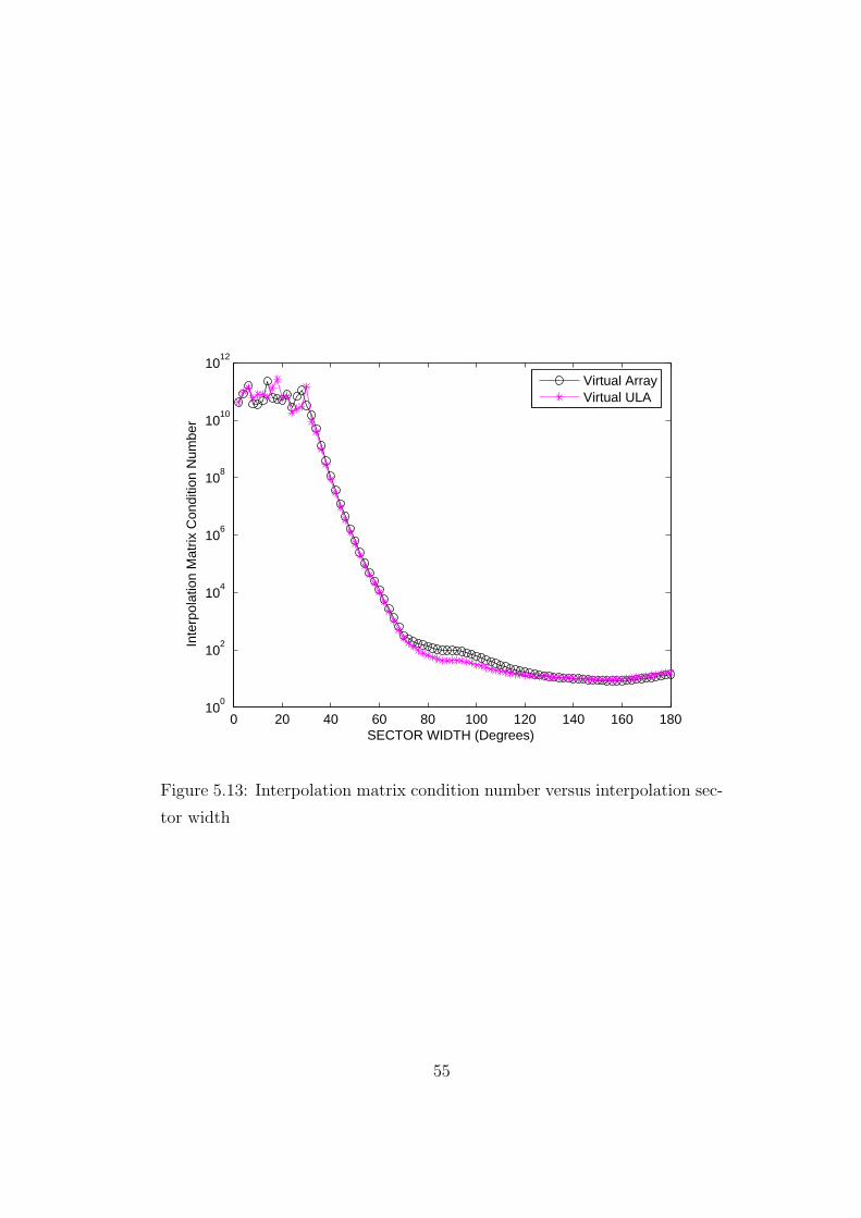
0 20 40 60 80 100 120 140 160 18010

0

102

104

106

108

1010

1012


Inte

rpol

atio

n M

atrix

Con

ditio

n N

umbe

r


Figure 5.13: Interpolation matrix condition number versus interpolation sec-

tor width

55

0 500 1000 1500 2000 2500 300010

−3

10−2

10−1

SECTOR PARTITION (Degrees)

Inte

rpol

atio

n Q

ualit

y F

robe

nuou

s N

orm


Figure 5.14: Frobenius norm ratio versus interpolation sector partition

56

0 500 1000 1500 2000 2500 300010

1

102

103

104

SECTOR PARTITION (Degrees)

Inte

rpol

atio

n M

atrix

Con

ditio

n N

umbe

r


Figure 5.15: Interpolation matrix condition number versus interpolation sec-

tor partition

choosen as 80o and the sector partition is changed from 15 to 3000. In Figure

5.14 the sector partition versus interpolation matrix condition number plot

is seen. It is concluded from the Figure that as the sector partition gets

larger, the condition number decreases. However, after some value the effect

is not very obvious. In Figure 5.15 the sector partition versus frobenius norm

ratio plot is seen. As the sector partition gets larger, the frobenius ratio de-

creases. However, after some value the effect is not very obvious. There is an

optimum sector partition value considering both the condition number and

frobenius norm. The designer can choose the optimum sector partition value

by plotting these Figures, before starting the interpolator design.

57

0 5 10 15 20 25 30 35 4010

−5

10−4

10−3

10−2

10−1

100

SNR (dB)

RM

SE

(D

egre

es)


Figure 5.16: Performances of two interpolation methods compared with CRB

for one source with DOA angle 58o. (Interpolation sector [45o 72o]).

One source at fixed DOA angle is created at 58o. SNR level is changed

from 0 dB to 40 dB. The interpolation sector for this simulation is chosen as

[45o 72o]. The DOA estimation RMSE versus SNR is plotted and compared

with the stochastic CRB for the two interpolation methods. . The result is

seen in Figure 5.16. As it is seen from the Figure the performances of two

interpolation methods are the same. In Figure 5.17 the same performance

curve is obtained for the interpolation sector [0o 180o]. The interpolation

sector effect is obvious.

58

0 5 10 15 20 25 30 35 4010

−5

10−4

10−3

10−2

10−1

100

101

102

SNR (dB)

RM

SE

(D

egre

es)



for one source with DOA angle 58o. (Interpolation sector [0o 180o]).

59

1

2

3

4

30

210

60

240

90

270

120

300

150

330

180 0

Sector BoundarySource DirectionSensor Position

58

63

Figure 5.18: The interpolation sector and the sources impinging on the real

array

5.1.2 Two Sources

Two equipower sources are created at fixed DOA angles 58o and 63o.

SNR level is changed from 0 dB to 40 dB. The interpolation sector for this

simulation is chosen as [45o 72o]. The interpolation sector and the sources

impinging on the array elements are seen in Figure 5.18. The DOA estimation

RMSE versus SNR is plotted and compared with the stochastic CRB for the

two interpolation methods.

In Figure 5.19 DOA estimation RMSE for the two interpolation methods

versus SNR compared with stochastic CRB is shown.

60

0 5 10 15 20 25 30 35 4010

−5

10−4

10−3

10−2

10−1

100

SNR (dB)

RM

SE

(D

egre

es)

Virtual Array

Virtual ULA

CRB


for two equipower uncorrelated sources with DOA angles 58o and 63o. (In-

terpolation sector [45o 72o]).

61

1

2

3

4

30

210

60

240

90

270

120

300

150

330

180 0

Sector BoundarySource DirectionSensor Position 58

6370


array

5.1.3 Three Sources

Three equipower sources are created at fixed DOA angles 58o, 63o and

70o. SNR level is changed from 0 dB to 40 dB. The interpolation sector

for this simulation is chosen as [45o 72o]. The interpolation sector and the

sources impinging on the array elements are seen in Figure 5.20. The DOA

estimation RMSE versus SNR is plotted and compared with the stochastic

CRB for the two interpolation methods.



62

0 5 10 15 20 25 30 35 4010

−5

10−4

10−3

10−2

10−1

100

SNR (dB)

RM

SE

(D

egre

es)



for three equipower uncorrelated sources with DOA angles 58o, 63o and 70o

.(Interpolation sector [45o 72o]).

63

5.2 Interpolated Spatial Smoothing

In this section the results of the simulations for the correlated sources

are presented. The simulations are performed in order to explore the perfor-

mance of the interpolated spatial smoothing algorithm applied with the two

interpolation methods. In all of the simulations, the performances are eval-

uated in the sense of root mean squared error and they are compared with

the stochastic Cramer-Rao lower bound (CRB) [13] calculated theoretically

for the original array. The experiments are performed for two, three and four

sources.

5.2.1 Two Sources

Two equipower sources are created at fixed DOA angles 58o and 63o. The

sources are correlated with correlation coefficient α = 0.7391 and β = 0.3061.

SNR level is changed from 0 dB to 40 dB. The interpolation sector for this

simulation is chosen as [45o 72o]. The interpolation sector and the sources

impinging on the array elements are seen in figure 5.22. The DOA estimation

RMSE versus SNR is plotted and compared with the stochastic CRB for the

two interpolation methods.



5.2.2 Three Sources

Three equipower sources are created at fixed DOA angles 45o, 60o and

115o and two of them are correlated with correlation coefficient α = 0.4,−0.3

and β = 0.8,−0.7. SNR level is changed from 0 dB to 40 dB. The interpo-

lation sector for this simulation is chosen as [20o 120o]. The interpolation

sector and the sources impinging on the array elements are seen in Figure

64

1

2

3

4

30

210

60

240

90

270

120

300

150

330

180 0


58

63


array

65

0 5 10 15 20 25 30 35 4010

−5

10−4

10−3

10−2

10−1

100

101

SNR (dB)

RM

SE

(D

egre

es)



for three equipower sources with DOA angles 58o, 63o and 70o one of which

is coherent with correlation coefficient α = 0.7391 and β = 0.3061 .(Interpo-

lation sector [45o 72o]).

66

1

2

3

4

30

210

60

240

90

270

120

300

150

330

180 0


45

60115


array

5.24. The DOA estimation RMSE versus SNR is plotted and compared with

the stochastic CRB for the two interpolation methods.


versus SNR compared with stochastic CRB is shown. For this case since the

interpolation sector is taken broad for low SNR values the RMSE is very high

compared to the stochastic CRB.

67

0 5 10 15 20 25 30 35 4010

−5

10−4

10−3

10−2

10−1

100

101

SNR (dB)

RM

SE

(D

egre

es)



for three equipower sources with DOA angles 45o, 60o and 115o two of which

are coherent with correlation coefficient α = 0.4,−0.3 and β = 0.8,−0.7

respectively .(Interpolation sector [20o 120o]).

68

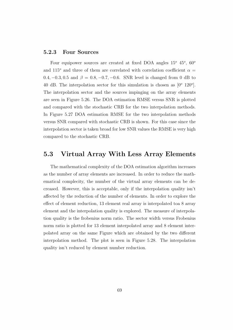
5.2.3 Four Sources

Four equipower sources are created at fixed DOA angles 15o 45o, 60o

and 115o and three of them are correlated with correlation coefficient α =

0.4,−0.3, 0.5 and β = 0.8,−0.7,−0.6. SNR level is changed from 0 dB to

40 dB. The interpolation sector for this simulation is chosen as [0o 120o].

The interpolation sector and the sources impinging on the array elements

are seen in Figure 5.26. The DOA estimation RMSE versus SNR is plotted

and compared with the stochastic CRB for the two interpolation methods.


versus SNR compared with stochastic CRB is shown. For this case since the

interpolation sector is taken broad for low SNR values the RMSE is very high

compared to the stochastic CRB.

5.3 Virtual Array With Less Array Elements

The mathematical complexity of the DOA estimation algorithm increases

as the number of array elements are increased. In order to reduce the math-

ematical complecity, the number of the virtual array elements can be de-

creased. However, this is acceptable, only if the interpolation quality isn’t

affected by the reduction of the number of elements. In order to explore the

effect of element reduction, 13 element real array is interpolated toa 8 array

element and the interpolation quality is explored. The measure of interpola-

tion quality is the frobenius norm ratio. The sector width versus Frobenius

norm ratio is plotted for 13 element interpolated array and 8 element inter-

polated array on the same Figure which are obtained by the two different

interpolation method. The plot is seen in Figure 5.28. The interpolation

quality isn’t reduced by element number reduction.

69

1

2

3

4

30

210

60

240

90

270

120

300

150

330

180 0


15

45

60115


array

70

0 5 10 15 20 25 30 35 4010

−5

10−4

10−3

10−2

10−1

100

101

102

SNR (dB)

RM

SE

(D

egre

es)



for four equipower sources with DOA angles 15o,45o, 60o and 115o three of

which are coherent with correlation coefficient α = 0.4,−0.3, 0.5 and β =

0.8,−0.7,−0.6 respectively .(Interpolation sector [0o 120o]).

71

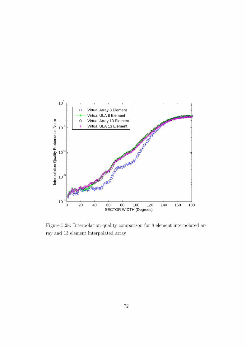
0 20 40 60 80 100 120 140 160 18010

−4

10−3

10−2

10−1

100


Inte

rpol

atio

n Q

ualit

y F

robe

nuou

s N

orm

Virtual Array 8 ElementVirtual ULA 8 ElementVirtual Array 13 ElementVirtual ULA 13 Element

Figure 5.28: Interpolation quality comparison for 8 element interpolated ar-

ray and 13 element interpolated array

72

chapter 6

conclusion

In this thesis, DOA estimation with interpolated array using root-MUSIC

algorithm for arbitrary array geometries has been examined. Two different

methods for designing interpolated array have been implemented. The two

methods differ in the selection of the virtual array. For arbitrary array ge-

ometry, two interpolation matrices are obtained within a sector using the

mentioned methods. The accuracies of the interpolators are investigated in

terms of the ratio of the frobenius norm of the interpolation error to the

frobenius norm of the array manifold matrix within the sector. It is observed

that both the two methods give almost the same interpolation quality and

the interpolation quality increases as the sector width decreases, however the

condition number of the interpolation matrix gets larger. The sector width

partition is another important thing that affects the interpolation error. As

the sector width partition gets larger the interpolation quality increases, how-

ever after at some value it is seen that it doesn’t result in any increase in

the interpolation quality. The simulation experiment for the interpolated

root-MUSIC using the two interpolation methods has seemed to result in

very similar results. They both give close values to the MUSIC algorithm

applied to real array geometry if the interpolator is designed properly. In

the virtual ULA method the design of the virtual array is under the con-

trol of the designer. The placement of virtual array elements is done by the

designer and generally the virtual elements are placed as close as possible

to the real elements. Another approach is to place array elements to the

73

perpendicular axis to the interested sector. However, the placement of this

type doesn’t result in an increase in the interpolator quality for arbitrary ar-

ray geometries which are almost linear. In the second interpolation method,

the designer can’t choose the virtual array elements, because the result of

virtual array method is not a physical array. It is a virtual array manifold

vector having the same differential behavior as the real array manifold vector

within the selected sector. Spatial smoothing algorithm is implemented and

the performance evaluation is done by using the two interpolation methods.

Spatial smoothing preprocessing performance was evaluated in an early work

by Friedlander [11] using virtual ULA. However, in this work spatial smooth-

ing is applied to a non-real virtual array having the necessary Vandermonde

structure and the same performance as in the virtual ULA case is obtained

in the simulations.

74

references

[1] A.J.Barabell“Improving the resolution performance of eigenstructure

based direction finding algorithms. ” Proc. ICASSP , pages 336-339,

Boston, MA, 1983

[2] M.S.Barlett, “Smoothing periodograms from time series with continuous

spectra ” Nature, 161:686-687,1948.

[3] G.Bienvenu and L.Kopp“Adaptivity to background noise spatial coher-

ence for high resolution passive methods. ” Proc. ICASSP, vol.1, pp.307-

310, Denver, Colorado, April 1980.

[4] G.Bienvenu and L.Kopp“Optimality of high resolution array processing

using the eigensystem approach. ” IEEE Trans. Acoustic, Speech, Signal

Processing, vol.ASSP-31, pp. 1234-1248, October 1983

[5] J.F.Bohme,“Estimation of spectral Parameters of correlated signals in

wavefields ” Signal Processing . vol.11, pp.329-337, 1986.

[6] M.Buhren, M.Pesavento and J.F.Bo hme“Virtual array design for array

interpolation using differential geometry” Proc.ICASSP’04

[7] J.Capon, “High resolution Frequency-Wavenumber Spectrum Analysis

” Proc. IEEE, 57(8):2408-1418,Aug. 1969.

[8] J.E.Evans, J.R.Johnson, and D.F.Sun “Application of advanced signal

processing techniques to angle of arrival estimation in ATC navigation

and surveillance system ” M.I.T Lincoln Lab, Lexington, MA, Rep. 582,

1982.

75

[9] B.Friedlander and A.J.Weiss, “Direction finding Using interpolated ar-

rays ” Report SPT-89-001-NE, Signal Processing Technology, February

1990.

[10] B.Friedlander, “Direction finding with an interpolated array ” in Proc.

ICASSP 90, Albuquerque, NM, pp.2951-2954 December 1990.

[11] Friedlander, B., Weiss, A.J., “Direction finding using spatial smoothing

with interpolated arrays ” IEEE Trans. on Aerospace and Electronic

Systems

[12] B.Friedlander“The root-MUSIC algorithm for direction finding with in-

terpolated arrays ” Signal Processing. vol.30, pp.15-29,1993 .

[13] A.B.Gershman and J.F.Bohme “A note on most favorable array ge-

ometries for DOA estimation and array interpolation . ” IEEE Signal

Processing Letters, vol.4 No.8, August 1997

[14] Gershman, A.B., Stoica, P., Pesavento, M. and Larsson, E.G., “Stochas-

tic Cramer-Rao bound for direction estimation in unknown noise fields,”

Radar, Sonar and Navigation, IEE Proceedings, vol.149, no.1, pp.2–8,

February 2002.

[15] P.Hyberg, M.Jansson and B.Ottersten“Array mapping:optimal trans-

formation matrix design” Proc.ICASSP’02, Orlando, Florida, pp.2905-

2908, May 2002 .

[16] T.J.Shan, T.Kailath and M.Wax “On spatial smoothing direction of

arrival estimation of coherent signals. ” IEEE Trans. on ASSP. ,

ASSP33(4) pages 806-811, August 1985

[17] A.Manikas,N.H.Dowlut“The use of differential geometry in array signal

processing ” Kybernetes vol.27, no.3, pp.251-163,1998 .

76

[18] Hyberg, P., Jansson, M., Ottersten, B., “Array Interpolation and DOA

MSE Reduction ” IEEE Trans. on Signal Processing, pp.4464 - 4471,

Vol. 53, No.12, Dec. 2005.

[19] A.Paulraj and T.Kailath“A subspace rotation approach to signal pa-

rameter estimation. ” Proc. IEEE , pages 1044-1045, July 1986

[20] S.U.Pillai, and B.H.Kwon“Forward/backward spatial smoothing tech-

niques for coherent signal identification ” IEEE Trans. Acoust., Speech,

Signal Processing, vol.37 ,no.1,pp.8-15, Jan. 1989.

[21] B.D.Rao and K.V.S.Hari, “Performance Analysis of Root-MUSIC ”

IEEE Trans. Acoustics Speech and Signal Processing, December 1989.

[22] R.Roy and T.Kailath “ESPRIT-Estimation of signal parameters via ro-

tational invariance techniques. ” IEEE Trans. on ASSP. , ASSP37(7)

pages 984-995, July 1989

[23] Scharf, L.L. and McWhorter, L.T., “Geometry of the Cramer-Rao

bound,”Statistical Signal and Array Processing, 1992. Conference Pro-

ceedings., IEEE Sixth SP Workshop on, pp.5–8, 7–9 October 1992

[24] R.O.Schmidt“Multiple emitter location and signal parameter estima-

tion. ” Proc. RADC Spectrum Estimation Workshop, Griffiths AFB,

Rome, New York, pp.243-258, 1979

[25] R.O.Schmidt Multiple emitter location and signal parameter estimation.

PhD Dissetatation, Stanford University, Stanford, California, 1981

[26] R.O.Schmidt“New mathematical tools in direction finding and spectral

analysis. ” Proc. SPIE 27th Ann. Symp., San Diego, California, August

1983.

77

[27] T.J.Shan, M.Wax, and T.Kailath “On spatial smoothing of estimation

of coherent signals ” IEEE Trans. Acoust., Speech, Signal Processing,

vol. ASSP-33,pp.806-811, Aug. 1985.

[28] Stoica, P. and Nehorai Arye, “MUSIC, maximum likelihood, and

Cramer-Rao bound,” Acoustics, Speech, and Signal Processing [see also

IEEE Transactions on Signal Processing], IEEE Transactions on, vol.37,

no.5, pp.720–741, May 1989.

[29] Stoica, P., Nehorai, A., “MUSIC, maximum likelihood, and Cramer-

Rao bound: further results and comparisons,” Acoustics, Speech, and

Signal Processing [see also IEEE Transactions on Signal Processing],

IEEE Transactions on, vol.38, no.12, pp.2140–2150, December 1990.

[30] Stoica, P., Jian Li, “Study of the Cramer-Rao bound as the numbers

of observations and unknown parameters increase,” Signal Processing

Letters, IEEE vol.3, no.11, pp.299–300, November 1996.

[31] Stoica, P., Larsson, E.G., Gershman, A.B. “The stochastic CRB for ar-

ray processing: a textbook derivation ” IEEE Signal Processing Letters,

pp.148-150, Vol. 8, Issue 5, May 2001

[32] Stoica, P. and Moses R., “Spectral Analysis of Signals.”Prentice-Hall,

Upper Saddle River, NJ, 2005.

[33] T.K. Yasar, “Improvements in DOA Estimation By Array Interpolation

in Non-Uniform Linear Arrays.”Thesis Work, METU, August 2006.

[34] Weiss, A.J. and Friedlander, B., “On the Cramer-Rao Bound for Direc-

tion Finding of Correlated Signals,”Signal Processing, IEEE Transac-

tions on [see also Acoustics, Speech, and Signal Processing, IEEE Trans-

actions on] vol.41, no.1, pp.495–, Jan 1993.

78

DIRECTION OF ARRIVAL ESTIMATION BY ARRAY ...DIRECTION OF ARRIVAL ESTIMATION BY ARRAY INTERPOLATION...

Documents

Transcript of DIRECTION OF ARRIVAL ESTIMATION BY ARRAY ...DIRECTION OF ARRIVAL ESTIMATION BY ARRAY INTERPOLATION...