Direct simulation of two-dimensional turbulent flow over a ...

INTERNATIONAL JOURNAL FOR NUMERICAL METHODS IN FLUIDSInt. J. Numer. Meth. Fluids 2007; 55:985–1018Published online 24 April 2007 in Wiley InterScience (www.interscience.wiley.com). DOI: 10.1002/fld.1503

Direct simulation of two-dimensional turbulent flowover a surface-mounted obstacle

V. P. Fragos1, S. P. Psychoudaki1 and N. A. Malamataris2,∗,†

1Department of Hydraulics, Soil Sciences and Agricultural Engineering, Aristotle University of Thessaloniki,GR-54124 Thessaloniki, Greece

2Department of Mechanical Engineering, Technological and Educational Institute of W. Macedonia,GR-50100 Kila, Greece

SUMMARY

Two-dimensional turbulent flow over a surface-mounted obstacle is studied as a numerical experimentthat takes place in a wind tunnel. The transient Navier–Stokes equations are solved directly with Galerkinfinite elements. The Reynolds number defined with respect to the height of the wind tunnel is 12 518.Instantaneous streamline patterns are shown that give a complete picture of the flow phenomena. Energyand enstrophy spectra yield the dual cascade of two-dimensional turbulence and the −1 power law decayof enstrophy. Mean values of velocities and root mean square fluctuations are compared with the avail-able experimental results. Other statistical characteristics of turbulence such as Eulerian autocorrelationcoefficients, longitudinal and lateral coefficients are also computed. Finally, oscillation diagrams ofcomputed velocity fluctuations yield the chaotic behaviour of turbulence. Copyright q 2007 John Wiley& Sons, Ltd.

Received 30 October 2006; Revised 3 March 2007; Accepted 11 March 2007

KEY WORDS: two-dimensional turbulence; energy and enstrophy spectra; calculation of autocorrelationand cross-correlation functions; Galerkin finite elements; chaos

1. INTRODUCTION

Turbulent flow over a surface-mounted obstacle is a fundamental problem in fluid mechanicshaving a wide range of applications in all domains of engineering science, as recently reviewed byFragos et al. [1], Larichkin and Yakovenko [2], Lohasz et al. [3]. Although the flow has receiveda lot of attention from the engineering community, it is still an open-ended problem partly due toits complicated geometry and partly due to the unresolved issues of turbulence.

∗Correspondence to: N. A. Malamataris, Department of Mechanical Engineering, Technological and EducationalInstitute of W. Macedonia, GR-50100 Kila, Greece.

†E-mail: nikolaos [email protected], [email protected]

Contract/grant sponsor: Office of the Hellenic Foundation for Research

Copyright q 2007 John Wiley & Sons, Ltd.

986 V. P. FRAGOS, S. P. PSYCHOUDAKI AND N. A. MALAMATARIS

The term surface-mounted obstacle is also ambigously used in the literature. By this term, someauthors mean a cubic or a prismatically shaped obstacle, where the fluid flows over the top andaround the sides. This is clearly a three-dimensional flow that takes place in the three-dimensionalspace. A recent solution to this problem using adaptive stabilized Galerkin finite elements withduality has been given by Hoffman and Johnson [4]. Other authors examine the flow over a cubicor a prismatically shaped obstacle having a width that extends up to the walls of a wind tunnel,where the obstacle is placed. This case is a two-dimensional flow, that takes place in the two-dimensional space, where any three-dimensional effect is generated from the existence of walls orfrom turbulence. This flow situation is the subject of this work.

For this particular flow, there is some recent experimental work in the turbulent regime conductedby Acharya et al. [5] and Larichkin and Yakovenko [2] for obstacles with rectangular cross-sectionof aspect ratio 1:1. There are also attempts to study this flow computationally by Acharya et al. [5],Hwang et al. [6] who used k–� models with a finite difference method and Lohasz et al. [3] whoapproached the problem with large eddy simulation and a finite volume method. In this work,the two-dimensional flow over a surface-mounted obstacle is studied computationally solving theunsteady Navier–Stokes equations in primitive variable formulation with standard Galerkin finiteelements. The experimental set-up and the process parameters of the study of Acharya et al. [5]are taken for comparison with the numerical results of this work.

Very recently, John and Liakos [7] studied the flow over a surface-mounted obstacle in thelaminar flow regime. They solved the transient Navier–Stokes equations directly focusing on theevolution of the reattachment points of the recirculating vortices, which develop downstream ofthe obstacle as a function of the slip coefficient. Psychoudaki et al. [8] made a complete studyof this flow using the same parameters as in the present work focusing on the first stages of itsdevelopment. They calculated the positions of separation and reattachment of vortices, the valueof shear stress and the growth of the boundary layer from the initiation of the flow up to theinception of turbulence.

Unlike other approaches in computational fluid mechanics, the finite element code of this workhas been verified by Fragos et al. [1] in the laminar flow regime with available experimental data.The results of that study have been used by John [9] and Oden and Prudhomme [10] for theevaluation of their numerical schemes. The ability of the code to correctly predict this flow atmoderate Reynolds numbers (order of 100) led the authors to use the following strategy in thestudy of two-dimensional turbulence: direct computation of turbulent flow may be simply viewedas the execution of an available laminar flow code at a higher Reynolds number by adding thetime derivative to the governing equations.

So far, two-dimensional turbulent flows have been primarily computed for bounded flows usingthe streamline vorticity formulation of the Navier–Stokes equations, as discussed in many reviewsincluding Kraichnan [11] and Nazarenko and Laval [12]. The primary interest of these works wasto predict the inverse energy cascade and the forward enstrophy cascade, which have been studiedtheoretically by Batchelor [13] and Kraichnan [11], who extended the work of Kolmogoroff intwo dimensions.

In the direct numerical simulation of three-dimensional flows, the Navier–Stokes equations aresolved in primitive variable formulation. As thoroughly discussed in many reviews of this subjectincluding Friedrich et al. [14], Moin and Mahesh [15] and Hunt et al. [16], all aspects of turbulencemay be studied with this method like cross-correlations, energy spectra, instantaneous versus meanfeatures of the flow along with computational issues like proper choice of initial conditions, inflowand outflow boundary conditions.

Copyright q 2007 John Wiley & Sons, Ltd. Int. J. Numer. Meth. Fluids 2007; 55:985–1018DOI: 10.1002/fld

DIRECT SIMULATION OF TWO-DIMENSIONAL TURBULENT FLOW 987

In this work, the issues of both two-dimensional turbulence and direct numerical simulation ofturbulent flows are addressed in the study of two-dimensional turbulent flow over a surface-mountedobstacle with square cross-section.

In the following, the governing equations are presented along with the computational domain andthe parameters of the flow. The issues of initial condition and inflow as well as outflow boundarycondition are examined next, followed by the finite element formulation and the computationaldetails. The results of this work are subsequently discussed and finally conclusions are drawn.

2. GOVERNING EQUATIONS AND FLOW PARAMETERS

The computational domain for the turbulent flow over a surface-mounted obstacle is shown inFigure 1. A Newtonian fluid of constant viscosity and density approaches with uniform u-velocitya wind tunnel of rectangular cross-section. At the entrance of the tunnel, the fluid is deceleratedalong the wall due to the no-slip boundary condition. The fluid continues its motion through thetunnel and hits the surface-mounted obstacle, which has a square cross-section. The flow separatesforming recirculation zones both upstream and downstream of the obstacle. The fluid leaves thecomputational domain after a certain distance downstream.

For a two-dimensional isothermal turbulent flow of an incompressible Newtonian fluid, thedimensionless Navier–Stokes equations are:

∇ ·u= 0 (1)

�u�t

+ u · ∇u= −∇ p + 1

Re∇{∇u + (∇u)T} (2)

u=0 v=0

8.6h

XY

0

u=0 v=0

u=0 v=0

u=Uo v=0

free boundary condition

wind tunnel exit

45h 1h 14h 3h

1h

wind tunnel entrance

Figure 1. Computational domain of the two-dimensional turbulent flow over a surface-mounted obstaclewith a square cross-section, placed in a wind tunnel.



The governing equations are given here in their primitive variable formulation. For two-dimensional turbulence, it is more common to use the streamline vorticity formulation. For thisflow, though, this formulation is not suitable, due to the singularity at the corners of the obstacle.The magnitude of vorticity goes to infinity there, as shear stress is infinite [17], which causesdivergence of any discretization scheme to be applied.

Equations (1) and (2) represent conservation of mass and momentum, respectively. Equation (2)is written in its stress divergence form [18, p. 362]. This choice is better suited for finite elements,because it leads to weak formulations in a more straightforward way than its simpler Lagrangianform.

The governing equations have been rendered dimensionless, by choosing the uniform approach-ing velocity of the fluid U0 as the characteristic velocity and the height of the obstacle h as thecharacteristic length. The reference time tr is then the ratio h/U0. In the governing equations,u= (u, v) is the velocity vector of the fluid with u and v its components in the x and y direction,respectively, t is the time, p is the pressure and Re=U0h/� is the Reynolds number with respectto the height of the obstacle, with � the kinematic viscosity of the fluid. The pressure p has beennon-dimensionalized with term �U 2

0 , with � being the density of the fluid. The time t has beennon-dimensionalized with reference time tr.

The dimensions of the computational domain and the Reynolds number were chosen to matchthe parameters of the laboratory experiment conducted by Acharya et al. [5]. In keeping withtheir conditions, the height of the obstacle is h = 6.35mm, the height of the tunnel is H = 9.6hand the approaching velocity of the fluid is U0 = 3.225m/s. Air was chosen as a working fluidwith a kinematic viscosity � = 1.57 · 10−5 m2/s and a density � = 1.2 kg/m3. These values of theprocess parameters yield a Reynolds number of 1304. It should be noted that the flow is in thefully turbulent regime, because the Reynolds number is 12 518 if it is computed using the heightof the tunnel H as a characteristic length. All the other dimensions of the computational domainare depicted in Figure 1 as functions of the height of the obstacle h.

In order to solve the problem, appropriate boundary and initial conditions must be chosen, whichare discussed in the next section.

3. BOUNDARY AND INITIAL CONDITIONS

The boundary conditions for this flow are depicted in Figure 1 and given in the equations below:

at the entrance:u =U0 (3)

v = 0 (4)

top and bottom boundaries, upstream the wind tunnel:u =U0 (5)

v = 0 (6)

top and bottom walls of the wind tunnel:u = 0 (7)

v = 0 (8)



along the walls of obstacle:u = 0 (9)

v = 0 (10)

at the outflow: free boundary condition

Equations (3) and (4) impose a uniform undisturbed velocity profile that defines the flow rateentering the wind tunnel. By choosing this boundary condition at the inlet, we avoid the introductionof any turbulent fluctuations numerically. In this way, the numerical experiment resembles theactual laboratory experiment regarding the initiation of turbulence, where the inlet velocity profileupstream of the wind tunnel is free of any disturbance, as it enters the test section. In this study, theonly source of turbulence is the disturbance of the fluid flow due to the presence of the obstacle.

This set-up of inlet boundary conditions is widely used in transient direct numerical simulationsof laminar flows [18, 19]. However, this concept is usually combined with white noise or inflowfluctuations when the flow is turbulent, in order to initiate turbulence in the calculation. In thiswork, we avoid any artificial initiation of turbulence by numerical means, which is also going tobe pointed out in the discussion of initial conditions that follows. Hoffman and Johnson [4, p. 10]also used this strategy (Equations (3) and (4)) in the flow past a square cylinder.

Equations (5) and (6) are tow tank boundary conditions. Equations (7)–(10) are no-slip boundaryconditions along the solid walls of the computational domain.

Special care must be taken at the outflow of the domain for turbulent flows, as thoroughlydiscussed by Friedrich et al. [14], Moin and Mahesh [15] and Le et al. [20], due to the fact thatvortical structures that are generated must travel downstream and leave the computational domainwithout any disturbance of the interior flow. This demand for suitable outflow boundary conditionsextends to other flow situations as well like compressible flows, as reviewed by Colonius [21],or laminar flows in unbounded domains, as discussed by Malamataris [22], Malamataris andPanastasiou [23], Panastasiou et al. [24], Sani and Gresho [25]. In general, the issue of the properboundary condition at the outflow of a computational domain is an open-ended problem for anytype of flow, since the magnitudes of the dependent variables are unknown a priori.

Common practice in the direct numerical simulation community is the use of convective bound-ary conditions at the outflow. This is in accordance with a Sommerfeld-type radiation boundarycondition that has already been used by Orlanski [26] in computations of atmospheric flows, wherethe computational domain is by definition unbounded. A different approach has been chosen byMalamataris [22] and Malamataris and Panastasiou [23] who used the free boundary condition, inorder to solve laminar free surface flows with convective waves that pass through the artificial out-flow. In the work of Papanastasiou et al. [24], it has also been shown that this boundary conditionperforms well in separated flows, where the recirculation region is cut at the outflow.

One may arrive at a similar condition called transparent outflow boundary condition by using aspecial Galerkin finite element method based on a variational formulation of the Navier–Stokes,as discussed by Ranacher [19, p. 12]. The transparent outflow boundary condition has beensuccessfully used by Hoffman and Johnson [4] in their study of three-dimensional turbulent flowsusing adaptive stabilized Galerkin finite elements.

The concept of the free boundary condition is used for this flow problem at the outflow of thecomputational domain (see Figure 1). However, it is beyond the scope of this work to go intothe details of the implementation of this idea or into its mathematical insight, which has beenaccomplished by Sani and Gresho [25], Heinrich and Vionnet [27], Griffiths [28] and Renardy [29].



Zienkiewicz and Taylor [30, vol. 3, p. 81] also suggest its use in their discussion about outflowboundary conditions in unbounded flows. It is impossible to express the free boundary conditionanalytically at this step, as is the case with traditional essential or natural boundary conditions,because this concept is derived from the weak form of the weighted Navier–Stokes residuals. First,the finite element method must be presented, in order to briefly outline its inclusion in the finalformulation of the equations to be solved and this is done in the next section.

Another major issue in the direct numerical simulation of turbulence is the choice of theproper initial condition, due to the high value of the Reynolds number. This issue is of generalinterest to the community of computational fluid mechanics, like the case of outflow boundaryconditions, because convergence may be impossible if the initial guess is far from the solution,even at steady-state problems of laminar flows with moderate Reynolds number (order of 100).However, the computational cost is low for steady-state problems and convergence to the desiredReynolds number is achieved with the incremental Reynolds number solution: a solution with alower Reynolds number is used as a first guess to a higher value of Reynolds and so on until thefinal solution.

This method is impossible in the direct simulation of turbulent flow. It is common practice togenerate random fluctuations superimposed on a computed or measured mean velocity field andlet the flow go until it reaches its final turbulent state, as discussed by Friedrich et al. [14]. Inaddition, this practice is enhanced either by imposing an inlet velocity profile in accordance withexperimental data [4, p. 12] or by using instantaneous results of large eddy simulation of channelflow [31, p. 927]. Although this procedure is effective and computationally economical, it hasthe disadvantage of introducing artificial physics in the computation. Even if turbulent flows getindependent of their initial conditions, there is a lack of elegance in this method.

A different approach has been taken in this work. The steady-state solution of laminar flowat Re= 1 was chosen as the initial condition. This numerical solution has been validated withlaboratory experimental data, in the work by Fragos et al. [1]. The streamlines for this flow areshown in Figure 2. By executing the computer program, the flow develops from its initial laminarstate to fully developed turbulence. Hence, this approach has the advantage that the transition fromlaminar to turbulent flow is also computed in addition to the study of turbulence, as is shown

Figure 2. Streamlines of the laminar flow over a surface-mounted obstacle at Reynolds number 1 withrespect to the obstacle height, chosen as the initial condition for this work. Details of the solution for this

flow are given in the work of Fragos et al. [1].



in Figures 4–7. In this way, the numerical experiment is in accordance with the experience ofexperimentalists who study flow phenomena at high Reynolds numbers by gradually adjusting theflow rate to the desired level. Additionally, any artificialities introduced numerically are avoided. Inthis way, the numerical experiment is closer to the real world. After all, turbulence may originatefrom instabilities of laminar flows, as discussed by Hunt et al. [16].

4. FINITE ELEMENT FORMULATION AND COMPUTATIONAL DETAILS

The computational mesh used in this work is shown in Figure 3. It consists of rectangular finiteelements of different sizes with nine nodes in each of them. Standard Galerkin finite elements[18, 30, 32] are used in this work to solve the governing equations along with the appropriate initialand boundary conditions. Velocities and pressure are approximated with quadratic �i and linear�i basis functions in each element as:

u =9∑

i=1ui�

i , v =9∑

i=1vi�

i , p=4∑

i=1pi�

i

Figure 3. (a) Computational mesh used in this work and (b) details of meshtessellation around the obstacle.



These approximations are inserted into Equations (1) and (2), which are weighted integrallywith basis functions �i and �i , respectively, in order to obtain the following continuity, Ri

C, andmomentum, Ri

M, residuals:

RiC =

∫V

∇ · u�i dV (11)

RiM =

∫V

[�u�t

+ u · ∇u − ∇ ·(

−pI + 1

Re{∇u + (∇u)T}

)]�i dV (12)

By applying the divergence theorem, in order to decrease the order of differentiation and projectpossible natural (Neumann type) boundary conditions, Equation (12) reduces to:

RiM =

∫V

[(�u�t

+ u · ∇u)

�i +(

−pI + 1

Re{∇u + (∇u)T}

)· ∇�i

]dV

−∫Sn ·

[−p I + 1

Re{∇u + (∇u)T}

]�i dS (13)

Since essential (Dirichlet type) boundary conditions for u and v are applied to all boundariesof the domain except for the outflow, Equation (13) is going to be replaced by Equations (3)–(10).The integral over the volume of Equation (13) along with Equation (11) are evaluated at all theinterior nodes of the computational domain. At the exit of the domain, the surface integral ofEquation (13) is added to all exit nodes, which is the application of the free boundary condition[22, 24].

In this way, the solution of the outflow is given by the governing equations without imposingany arbitrary boundary condition, which distorts the physics of the flow there and may propagateinto the interior of the domain. In order to examine the error that is introduced in the code atthe outflow, it is common practice to run the computer code at domains with shorter lengths andcheck how velocity and pressure fields change. This study has been done in this work and resultsexamining how the accuracy of the solution is affected by the outflow boundary condition aregoing to be discussed in the next section.

Equations (11) and (13) represent an algebraic system of nonlinear equations, which is solvedwith a Newton–Raphson iterative scheme. The convergence criterion imposed on the Newton–Raphson iteration was 10−6 for velocities and 5·10−4 for pressure. Gauß elimination is used forthe inversion of the Jacobian matrix, which is formed by differentiating the residuals Ri

C andRiM with respect to the nodal unknowns ui , vi and pi . In Table I, the coordinates of the mesh

are given at every point of the computational domain. The finite element program was written inFORTRAN 77. Time integration was performed with the backward Euler method. At each timestep, three iterations were necessary for code convergence. It should be noted that the convectiveterms of the Navier–Stokes equations are dominant for this flow. However, stabilization of theseterms was unnecessary, because the mesh used was irregular and denser at locations around theobstacle where stabilization issues may be of importance. After all, our experience with standardGalerkin finite elements shows that any sort of numerical instabilities may be cured by refiningthe mesh.

All results presented in the next section are independent of time step and mesh resolution. Inorder to determine this independence of results due to discretization, the code was run with a



Table I. Data of computational mesh of Figure 3.

Number of elements 14 645Number of nodes 59 299Number of unknowns 133 603CPU time per iteration 3minComputer used Pentium (R) 4 CPU 2.66GHz 1.00GB RAMLocation of obstacle 14�x�15Height of obstacle 0�y�1Time step 0.01

x-coordinate−3.0,−2,−1,−0.5,−0.25,−0.125,0.0,0.125,0.25,0.5,0.75,1,1.25,1.5,1.75,2,2.25,2.5,2.75,3,3.5,4,4.5,5,5.5,6,6.5,7,7.5,8,8.5,9,9.510,10.5,11,11.5,12,12.2,12.4,12.6,12.8,13,13.1,13.2,13.3,13.4,13.45,13.5,13.55,13.6,13.65,13.7,13.75,13.8,13.85,13.90,13.95,13.96,13.97,13.98,13.99,14,14.01,14.02,14.03,14.04,14.05,14.10,14.15,14.20,14.25,14.30,14.35,14.40,14.45,14.50,14.55,14.60,14.65,14.70,14.75,14.8,14.85,14.90,14.95,14.96,14.97,14.98,14.99,15,15.01,15.02,15.03,15.04,15.05,15.1,15.15,15.2,15.25,15.3,15.35,15.4,15.45,15.5,15.6,15.7,15.8,15.9,16,16.1,16.2,16.3,16.4,16.5,16.6,16.7,16.8,16.9,17,17.1,17.2,17.3,17.4,17.5,17.6,17.7,17.8,17.9,18,18.1,18.2,18.3,18.4,18.5,18.6,18.7,18.8,18.9,19,19.1,19.2,19.3,19.4,19.5,19.6,19.7,19.8,19.9,20,20.1,20.2,20.3,20.4,20.5,20.6,20.7,20.8,20.9,21,21.1,21.2,21.3,21.4,21.5,21.6,21.7,21.8,21.9,22,22.1,22.2,22.3,22.4,22.5,22.6,22.7,22.8,22.9,23,23.1,23.2,23.3,23.4,23.5,23.6,23.7,23.8,23.9,24,24.1,24.2,24.3,24.4,24.5,24.6,24.7,24.8,24.9,25.0,25.1,25.2,25.3,25.4,25.5,25.6,25.7,25.8,25.9,26,26.1,26.2,26.3,26.4,26.5,26.6,26.7,26.8,26.9,27,27.1,27.2,27.3,27.4,27.5,27.6,27.7,27.8,27.9,28,28.1,28.2,28.3,28.4,28.5,28.6,28.7,28.8,28.9,29,29.1,29.2,29.3,29.4,29.5,29.6,29.7,29.8,29.9,30,31,32,33,34,35,36,37,38,39,40,41,42,43,44,45,46,47,48,49,50,51,52,53,54,55,56,57,58,59,60.

y-coordinate0,0.01,0.035,0.06,0.085,0.11,0.14,0.2,0.3,0.35,0.40,0.45,0.50,0.55,0.60,0.65,0.70,0.75,0.8,0.85,0.9,0.95,0.97,0.98,0.99,1,1.005,1.01,1.02,1.03,1.04,1.05,1.06,1.1,1.25,1.5,1.75,2,2.33,2.67,3,4,5,6,7,8,8.5,8.75,9,9.1,9.2,9.3,9.4,9.5,9.55,9.6.



denser mesh by doubling the number of elements in the x and y direction and with a finer timestep by reducing the time step given in Table I to half. The output was compared to the resultsobtained for the time and space discretization given in Table I. Regarding the accuracy of the meshdiscretization, the results are shown in the next section following the discussion of the influenceof the outflow boundary conditions.

It should be noted that the Kolmogoroff scale, which is of the order of 0.1mm, is approximatelysatisfied in the vicinity of the obstacle. However, as pointed out by Moin and Mahesh [15], accurateresults in turbulent flows may be obtained with mesh resolutions which have length scales of theorder of magnitude of Kolmogoroff’s scales. From a computational point of view, it is irrelevantif theoretical length scales are resolved, as long as the results are independent of the discretizationerror of the numerical scheme. After all, it may be possible that even mesh resolutions withscales smaller than Kolmogoroff’s produce mesh-dependent results, depending on the type of flowunder consideration. The ultimate judgement though for the accuracy of computational resultsis the comparison with the available laboratory experimental measurements and the test whetheruniversal turbulent characteristics are validated, which is discussed in the next section.

5. RESULTS AND DISCUSSION

In the following discussion, mean values of the flow variables are computed in the standardway as

u = 1

T

∫ t0+T

t0u dt

with t0 = 150, T = 350 and u the instantaneous value of the flow variable. The transition period forthis flow is 140 dimensionless time units (see Figures 4–7 and 12–15). Additionally, data taken fora period of 350 dimensionless time units are enough, in order for the mean values of the flow toobtain statistically stationary values. At every time step of the calculation, the solution was stored,so that 35 000 numerical data points were available for the analysis of the results. Simpson’s rulehas been used for the evaluation of the above-mentioned integral. The fluctuations u′ are calculatedthen as

u′ = u − u

The instantaneous values u of the flow variables have been obtained from the direct computationof the governing equations with the boundary and initial conditions given in the previous sections.Instantaneous properties, mean values and fluctuations of the flow field are discussed next andtheir interactions are elucidated.

5.1. Instantaneous streamlines of the flow

Instantaneous streamlines are shown at selected time steps in Figures 4–7. In the beginning of theflow, the recirculation region increases downstream of the obstacle, until it becomes big enoughand breaks into two parts. One part is attached to the downstream side of the obstacle and theother part is a vortical structure that travels downstream. As time advances, this phenomenon ofgrowth of the recirculation region until it breaks into two parts continues incessantly, since theflow rate is constant at the inlet.



Figure 4. Computed streamlines that describe the development of turbulent flow in the first 50 time units.

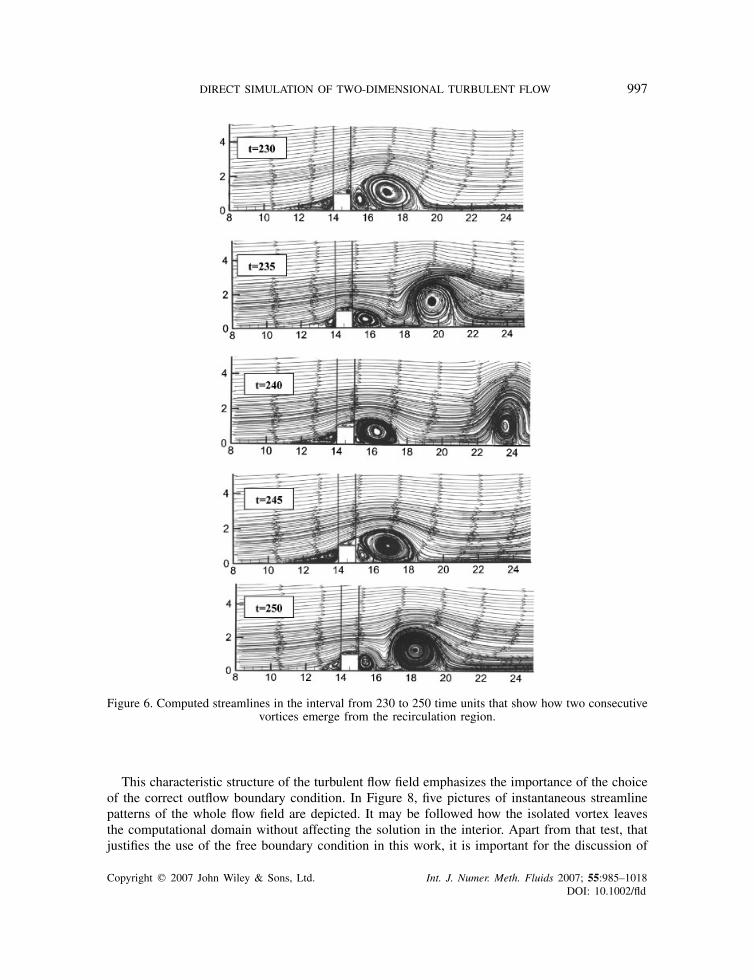
The transition period for this flow is depicted in Figures 4 and 5 up to time t = 140. During thistime, the regular, laminar, initial flow configuration is transformed to a fully developed turbulentflow. In Figure 6, shorter time intervals of the streamline patterns are shown, so that the readercan follow how two consecutive vortices break from the recirculation region downstream of theobstacle and continue travelling. The time needed for one vortex to be generated is between 15and 20 dimensionless time units. The exact time is going to be calculated later in the discussion ofthe oscillograms of the fluctuations. Additional streamline patterns are shown up to the last timestep of our calculation for this flow in Figure 7.



Figure 5. Computed streamlines in the interval from 80 to 200 time units that show the endof the transition from laminar to turbulent flow and the beginning of the generation of the

isolated vortices, that travel downstream.

The travelling of the isolated vortices downstream is reminiscent of the von Karman vortexstreet as also pointed out by John and Liakos [7], who studied this phenomenon at laminar flowconditions. Due to the constant production of these isolated vortices, a series of four can beobserved in the downstream distance of the computational domain, as shown in Figure 8. It shouldbe noted though, that in the case of the flow around a cylinder these vortical structures appear if theflow field is calculated with the velocity of the mean flow. In our study, the vortices appear in theinstantaneous snapshots of the streamlines in Figures 4–8, due to the fact that they are producedon the surface of the wall and they move downstream carried by the flow.



Figure 6. Computed streamlines in the interval from 230 to 250 time units that show how two consecutivevortices emerge from the recirculation region.

This characteristic structure of the turbulent flow field emphasizes the importance of the choiceof the correct outflow boundary condition. In Figure 8, five pictures of instantaneous streamlinepatterns of the whole flow field are depicted. It may be followed how the isolated vortex leavesthe computational domain without affecting the solution in the interior. Apart from that test, thatjustifies the use of the free boundary condition in this work, it is important for the discussion of



Figure 7. Computed streamlines in the interval from 255 to 500 time units that show the periodic natureof the constant generation of isolated vortices and the consecutive growth of the recirculation region until

it breaks again and becomes smaller and grows and so on.

the results that follow to know in detail if and how much the velocity profiles are distorted in thevicinity of the outflow.

For this purpose, the computer code was run with a computational domain 10 units of lengthshorter than the regular domain given in Figure 1. This procedure is the standard way to inves-tigate whether an outflow boundary condition works well, as thoroughly discussed by Sani andGresho [25]. The results are shown in Figure 9. The regular domain is termed long domain in thatfigure, in order to distinguish it from the shorter domain. The profiles of u- and v-velocity of theseruns at positions x = 40, 45, 50 of the short domain are compared to the corresponding profilesobtained from the long domain at the same x-coordinate. There is some discrepancy of 10% in the



Figure 8. Computed streamlines in the interval from 316 to 324 time units that show how an isolatedvortex leaves the computational domain without any distortion of the flow phenomena in the interior.

u- and v-profiles at the exit of the short domain (x = 50), which diminishes to 5% for the profilesat x = 45. Finally, at 10 units of length upstream of the outflow of the short domain (x = 40), theresults for the profiles of both velocity components are practically identical. This result means thatat least at 10 units of length upstream of the regular domain (at x = 50 in Figure 3), the analysisof instantaneous magnitudes of the velocity and its fluctuations are completely unaffected by anyunavoidable inaccuracies caused due to the artificial outflow boundary.

It should be noted that the flow phenomena are very intense in the computational domain upto the exit, although the contrary may have been expected as the distance from the downstreamside of the obstacle increases. This persistent existence of vortices downstream of the obstacle is



0

1

2

3

4

5

6

7

8

9

-0.2 0.2 0.6 1 1.4

u

x=40

0

1

2

3

4

5

6

7

8

9

-0.2 0.2 0.6 1 1.4

u

x=45

0

1

2

3

4

5

6

7

8

9

-0.2 0.2 0.6 1 1.4 1.8

u

x=50

0

1

2

3

4

5

6

7

8

9

-0.6 -0.4 -0.2 0 0.2V

y

x=40

0

1

2

3

4

5

6

7

8

9

-0.6 -0.4 -0.2 0 0.2 0.4 0.6V

y

x=45

0

1

2

3

4

5

6

7

8

9

-0.6 -0.4 -0.2 0 0.2 0.4 0.6V

y

y y y

long

short

x=50

longshort

Figure 9. Comparison of u- and v-velocity components at three different locations between thelong (60 units of length) and the short (50 units of length) domain that sheds more light to the

performance of the free boundary condition at the outflow of the computational domain.



x=15

0

1

2

3

4

5

6

7

8

9

-0.2 0.4 1 1.6u

x=20

0

1

2

3

4

5

6

7

8

9

-0.2 0.4 1 1.6u

yy

x=30

0

1

2

3

4

5

6

7

8

9

-0.2 0.4 1 1.6u

y

x=40

0

1

2

3

4

5

6

7

8

9

-0.2 0.4 1 1.6u

y

x=50

0

1

2

3

4

5

6

7

8

9

-0.2 0.4 1 1.6u

y

regular

dense

Figure 10. Study of mesh independence. The mesh used in this work is termed regular mesh(see Table I). Dense mesh is the discretization by doubling the elements in both the x- and

y-directions of the regular mesh.

analogous to the well-known fact that the von Karman vortex street continues undisturbed even at70 diameters downstream the cylinder, as observed by Taneda [33].

From a computational point of view, the outflow should be chosen at a distance where theintensity of the fluctuations and vortical structures diminishes. However, this is not the case forthis flow, due to the continuous production of vortices and the nature of turbulence. Other conceptsfor outflow boundary conditions should be developed for such cases. It is interesting that the freeoutflow boundary condition performs well for such a flow situation, since this concept has beendeveloped for laminar flow problems and used successfully in other applications [1, 34, 35], wherethe flow was far from turbulence.

The results of the study of the mesh independency of the numerical solution are shown inFigure 10. Regular mesh is termed the tessellation of the domain given in Table I. Dense meshis termed the discretization of the domain by doubling the finite elements of the regular meshin both x- and y-direction. The results for both mesh tessellations are indistinguishable up tox = 20, that is five units of length downstream of the obstacle. At position x = 30, there is somediscrepancy in the region 0.5<y<3. The results are again almost indistinguishable at the otherx-positions in the figure. The locations shown in Figure 10, have been chosen, because the analysisof the statistical characteristics of turbulence is going to be made at the same x-coordinates aty = 5 (Figures 12–18). The comparison of the numerical results with the available experimentaldata is done at locations x�22.1 (Figures 21–25). That is, in the analysis that follows, all ournumerical results are mesh independent. It should be noted that the results of the v and p profilesare analogous to the u profiles shown in Figure 10. The numerical results are also independentof the time step chosen. The discussion of this study is omitted, since, in all cases, the profilesare similar to the profiles at x�20 of Figure 10. We avoided comparing mesh independence bylooking at averaged profiles, since averaging damps the instantaneous picks in the magnitudes ofvelocities, as is going to be shown in the following discussion of the mean streamlines of the flow.



Figure 11. (a) Computed streamlines with the mean values of the velocity components in the wholedomain and (b) details of the vortical structures in the vicinity of the obstacle that show how the physics

of the flow are completely smoothened if mean properties are considered.

5.2. Mean streamlines of the flow

It is common practice in turbulent research to present results by computing mean values of theflow variables. The streamline pattern of the mean flow field is shown in Figure 11. By comparingthis figure with any instantaneous flow field given in Figures 4–8, it is clearly shown that thereis a striking difference in the physics. All isolated vortices are completely absorbed in Figure 11and the recirculation region is smoothened. There is no indication of the intense flow phenomenain the immediate region downstream of the obstacle that cause growth and separation of vortices.

This discrepancy between instantaneous and mean streamline patterns justifies the study ofturbulence by means of a direct computation of the Navier–Stokes equations, since flow phenomenamay be completely distorted if only mean values of the flow variables are calculated. Certainly, thework of Reynolds, Prandtl and other exceptional engineers, mathematicians and physicists in fluidmechanics has been very influential from late 19th century up to this date, so that any analysis ofturbulent calculations even now should refer to some standards, that they established. However,the direct computation of turbulent flows gives—besides laboratory experiments—a deeper insightinto the physics of flow phenomena than any other theoretical or computational effort, which isbased on the analysis of mean values or statistical properties.

5.3. Velocity fluctuations

Oscillograms of u- and v-velocity fluctuations are shown in Figures 12–15 at various locationsof the flow domain. In all these figures, the y-coordinate was kept constant at y = 5 and thex-coordinate was varied from 20 to 50. At point (x = 20, y = 5), which is relatively close to the



Figure 12. Oscillations of the fluctuations of both velocity components at point (x = 20, y = 5) of thecomputational domain. The signals seem to be almost periodic after the transition period from the initial

laminar flow condition to fully developed turbulence.

obstacle (5 units of length downstream of the trailing edge), the fluctuations are completely regularafter a certain transition period of 75 units of time. This regularity in the signal is due to theconstant generation of vortices downstream of the obstacle, as shown in Figures 4–8. The onlysource of turbulence here is the disturbance of the flow due to the presence of the obstacle. Itis expected that turbulence is still undeveloped in the immediate vicinity of the obstacle. Thecomputed result should be an almost periodical oscillogram of the fluctuations for both velocitycomponents, as is actually shown in Figure 12. The period of oscillation is 16.7 dimensionlesstime units. This value corresponds to the time taken for one vortex to break from the recirculationregion, which has already been approximately estimated in the discussion of Figure 6.

Further downstream at point (x = 30, y = 5) in Figure 13, the oscillograms of the fluctuationsare almost as regular as in the previous picture, although there is a certain randomness in theminima and maxima of the signal especially for the fluctuation of the v-component of the velocity.



Figure 13. Oscillations of the fluctuations of both velocity components at point (x = 30, y = 5)of the computational domain. The signals exhibit a weak randomness in the maxima and the

minima after the transition period.

Another difference with Figure 12 is that the transition period lasts about 100 units of time, sinceit takes more time for the initial disturbance to reach this point.

In Figures 14 and 15 at points (x = 40, y = 5) and (x = 50, y = 5), respectively, the situationis completely different. The flow develops turbulent characteristics in a much more pronouncedfashion. The result is a randomness in the oscillograms of the velocity fluctuations superimposedon the periodicity due to the steady generation of vortices. This randomness is exhibited in theacanonical variation of the minima and the maxima of the amplitude of the oscillations. The periodof the oscillation is undisturbed, though, as it should be, due to the periodic nature of the flow atthis Reynolds number. Additionally, randomness is also observed within each period of oscillation,where the pattern of the fluctuations is different and acanonical as well. This difference in thepattern may not be obvious at a first glance, due to the dominant periodical nature of the signal.However, the randomness in the pattern exists and gives the message that turbulence develops as



Figure 14. Oscillations of the fluctuations of both velocity components at point (x = 40, y = 5) ofthe computational domain. The signals exhibit a stronger randomness in the maxima and the minima

as the flow continues downstream.

the flow is distanced from the obstacle. Especially Figure 15 is reminiscent of the signals takenby many experimentalists over the last 80 years and shown in standard books of turbulence [36,p. 499; 37, p. 28; 38, p. 12], in order to invoke the intuition of the reader about the complicatednature of turbulent flow and justify the attitude of many workers in the field towards a statisticalanalysis of turbulence.

In this work, it is shown that deterministic spatiotemporal chaos is predicted by directly solvingthe Navier–Stokes equations. To the best of our knowledge, this kind of oscillograms is shownfor the first time from a computational analysis. So far, even in books dealing with chaos, chaoticbehaviour has been limited to the subject of solving equations, where the dependent variablesare only a function of time (e.g. [39]). It should be also noted that this behaviour of velocityfluctuations at the points shown in Figures 12–15 is representative of any other point in the flowdomain with coordinates (x, y0), where y0 is kept at a constant value.



Figure 15. Oscillations of the fluctuations of both velocity components at point(x = 50, y = 5) of the computational domain. The signals exhibit a total randomness which

is a fundamental characteristic of turbulence.

5.4. Energy and enstrophy spectra

It is customary in turbulent research to study the energy and enstrophy spectra of the instantaneousvalues of velocities and vorticity. Especially, the energy spectrum has been the subject of extensiveexperimental investigation and has led to an empirical law that has been verified by the deeplyinfluential work of Kolmogoroff, as thoroughly discussed by Frisch [37]. Batchelor [13] andKraichnan [11] extended these ideas to two-dimensional turbulence. They found that the energyspectrum follows both the − 5

3 power law of three-dimensional turbulence (called inverse energycascade in the terminology of two-dimensional turbulence) and the −3 power law, which has beenattributed to a forward enstrophy cascade. Additionally, they studied the enstrophy cascade andpredicted a −1 power law for the dependency of enstrophy with respect to the frequency of thespectrum.

The energy spectra are shown in Figures 16 and 17. They have been calculated at the samepoints as the oscillograms of the velocity fluctuations in Figures 12–15 using a specially developed



Figure 16. Energy spectra of the kinetic energy of the u-velocity component at four different locations ofthe computational domain. The calculations have been performed with the commercial program Labview.

The dual cascade of two-dimensional turbulence is validated.

computer code based on LabView, the commercial data processing computer software providedby the National Instruments Corporation. A common characteristic of all the graphs in thesefigures is the spike at 30Hz, which is attributed to the periodical nature of the generation ofvortices downstream of the obstacle. This frequency corresponds to the period of oscillations inFigures 12–15, which is 16.7 dimensionless time units. The reference time h/U0 is 1.96ms, sothat the period of oscillations obtains the value 32.88ms. Finally, the inverse of the period is30.4 Hz, which is the frequency of the spike. This agreement between the observations of theinstantaneous streamline patterns, the computation of the oscillograms of the velocity fluctuationsand the spectral analysis of these signals provides an additional argument for the reliability of thenumerical results of this work.

In Figure 16, the energy spectrum of the u-velocity at point (x = 20, y = 5) has strong depen-dencies on both the − 5

3 and the −3 power law of the frequency. As the flow continues downstream,the − 5

3 power law appears in a much wider frequency range than the −3 power law especiallyat point (x = 40, y = 5). In Figure 17, the energy spectrum of the v-velocity component at point



Figure 17. Energy spectra of the kinetic energy of the v-velocity component at four different locations ofthe computational domain. The calculations have been performed with the commercial program Labview.

The dual cascade of two-dimensional turbulence is validated.

(x = 20, y = 5) shows a clear −3 dependency on frequency of almost two orders of magnitudewhile the − 5

3 dependency is limited to the region from 30 to 100Hz. As the flow continuesdownstream, the dependency of the energy spectrum on frequency is equally divided in both the− 5

3 and the −3 power law. In any case, the dual cascade of two-dimensional turbulence is clearlydemonstrated in all the results of Figures 16 and 17, even though the velocity fluctuations showthat turbulence is less pronounced up to point (x = 30, y = 5).

The enstrophy spectra for this flow are shown in Figure 18 at the same points as the energyspectra. The enstrophy was calculated as one half of the square of vorticity. At point (x = 20, y = 5),the −1 power law in the decay of enstrophy extends more than one order of magnitude. Up to point(x = 40, y = 5), this decay is gradually limited to a narrower region. Further downstream, the −1power law covers again one order of magnitude in the frequency range at point (x = 50, y = 5).The agreement of the results of the spectral analysis of this work with theoretical results of two-dimensional turbulence confirms the accuracy of the numerical predictions. The slopes − 5

3 and −3are included in Figures 16–18, so that the reader may estimate how far or close is the frequencydependence of the kinetic energy from these well-known laws.



Figure 18. Enstrophy spectra at four different locations of the computational domain. The calculationshave been performed with the commercial program Labview. The decay of enstrophy with the −1 power

law validates the direct enstrophy cascade of two-dimensional turbulence.

5.5. Statistical properties of the flow

Correlation functions are useful tools in studying the spatial structure of turbulence from a statisticalpoint of view. Three correlation functions are calculated in this work with the following definitions:

R(�) = 1

T

∫ t0+Tt0

u′(t)u′(t + �) dt

u′2(t), Ru(y)= 1

T

∫ t0+Tt0

u′(x, y0)u′(x, y0 + y) dt

u′2(x, y0)

Rv(y)= 1

T

∫ t0+Tt0

v′(x, y0)v′(x, y0 + y) dt

v′2(x, y0)



-0.4

-0.2

0.0

0.2

0.4

0.6

0.8

1.0

1.2

0 20 40 60 80 100 120 140

R(

)

Figure 19. The Eulerian autocorrelation function at point (x = 50, y = 5) calculated from the computedfluctuations of the u-velocity component.

-0.8

-0.6

-0.4

-0.2

0.0

0.2

0.4

0.6

0.8

1.0

1.2

1.4

4 4.5 5 5.5 6 6.5 7 7.5 8 8.5 9 9.5

y-coordinate

Rv(x.y)

Ru(x.y)

Rv(x.y)Ru(x.y)

x=50

Figure 20. The longitudinal Ru(y) and lateral Rv(y) cross-correlation functions calculated from thecomputed fluctuations of the u- and v-velocity components, respectively, with fixed point (x = 50, y0 = 4)and variation along the y-coordinate of the computational domain up to the upper wall of the wind tunnel.

R(�) is the Eulerian autocorrelation function that relates the fluctuation of the u-velocity compo-nent at a certain point of the flow domain to the fluctuation of the same velocity component at thesame point at a later time. Ru(y) is the longitudinal correlation function that relates the fluctuationof the u-velocity component at a certain point of the flow field and time to the fluctuation of thesame velocity component at a different point in the y direction of the flow field at the same time.Rv(y) is the lateral correlation function that relates the fluctuation of the v-velocity component inthe corresponding way as Ru(y). The values of t0 and T have been given in the beginning of thissection. All three integrals have been calculated with Simpson’s rule.



0

1

2

3

4

5

6

7

8

9

-0.2 0.3 0.8 1.3

x=13.6

0

1

2

3

4

5

6

7

8

9

0 0.5 1 1.5

x=14.5

0

1

2

3

4

5

6

7

8

9

-0.2 0.4 1 1.6

x=15.0

0

1

2

3

4

5

6

7

8

9

-0.4 0.2 0.8 1.4

yyy

y y

yyy y

x=15.4

0

1

2

3

4

5

6

7

8

9

-0.4 0.2 0.8 1.4

x=15.6

0

1

2

3

4

5

6

7

8

9

-0.8 -0.1 0.6 1.3

x=17.2

0

1

2

3

4

5

6

7

8

9

-0.4 0.1 0.6 1.1

x=18.8

0

1

2

3

4

5

6

7

8

9

0 0.5 1 1.5

x=20.4

0

1

2

3

4

5

6

7

8

9

0 0.5 1 1.5

Acharya et al

this work

x=22.1

u uu u

u u uu u

Figure 21. Comparison of calculated mean u-velocity profiles versus laboratory data obtained byAcharya et al. (1994) at various locations of the computational domain.

The autocorrelation function R(�) at point (x = 50, y = 5) is shown in Figure 19. The dimen-sionless time difference � goes up to 150 time units. R(�) has been evaluated at each time stepyielding 15 000 points for the calculation of the curve in Figure 19. The autocorrelation functionstarts at 1, diminishes gradually, obtains negative values and finally tends to zero. This is a typicallymeasured curve indicative of the randomness of the signal, which has already been observed inFigure 15.

The longitudinal and lateral correlation functions at point (x=50, y0=4) are shown in Figure 20.The variation in the y-coordinate goes up to the upper wall of the wind tunnel of the computationaldomain (see Figure 1). Both correlation functions start from 1 and gradually diminish. The functionRu(y) obtains appreciable negative values like R(�) and finally both cross-correlations becomezero at the wall due to the no-slip boundary condition there. In the literature [36, p. 579; 40, p. 556],it is stated that the analysis depicted in Figure 20 is rarely done experimentally, because many



0

1

2

3

4

5

6

7

8

9

-0.1 0.1 0.3 0.5

x=13.6

0

1

2

3

4

5

6

7

8

9

-0.1 0.1 0.3 0.5

x=14.5

0

1

2

3

4

5

6

7

8

9

-0.1 0.1 0.3 0.5

x=15.0

0

1

2

3

4

5

6

7

8

9

-0.1 0.1 0.3 0.5

x=15.4

0

1

2

3

4

5

6

7

8

9

-0.1 0.1 0.3 0.5

x=15.6

0

1

2

3

4

5

6

7

8

9

-0.3 0 0.3 0.6

y

x=17.2

0

1

2

3

4

5

6

7

8

9

-0.3 0 0.3 0.6

y

x=18.8

0

1

2

3

4

5

6

7

8

9

-0.3 0 0.3 0.6

yx=20.4

0

1

2

3

4

5

6

7

8

9

-0.2 0 0.2 0.4

y

y y y y y

Acharya et al

this work

x=22.1

vvv v v

v v v v

Figure 22. Comparison of calculated mean v-velocity profiles versus laboratory data obtained byAcharya et al. (1994) at various locations of the computational domain.

measurements are required. However, in the direct computation of turbulent flows this analysis isas straightforward as the calculation of autocorrelation functions, since at every time step of thecomputation all values of the flow variables in the flow field are obtained, stored and postprocessedas desired.

Although, all three correlation functions are unable to contribute to the understanding of thephysics of turbulence, they provide an accurate test for the quality of the computational results.These functions simply examine whether events that take place spatially or temporally away froma fixed point in space or time correlate in an increasingly fading fashion, as it should actually befor a random process, according to common sense. The computational results of this work satisfythis requirement of statistical analysis and verify the chaotic behaviour of the oscillograms of thevelocity fluctuations shown in Figures 12–15.

The results of the statistical analysis along with the spectra are consistent with the chaoticnature of the oscillograms in Figures 12–15, which proves, that the tessellation of the domainis adequate for this flow. Certainly, by studying this flow at even higher Reynolds numbers, the



0123456789

-0.1 0.1 0.3 0.5

yx=13.6

01

23

456

78

9

-0.1 0.1 0.3 0.5

y

x=14.5

0

1

2

3

4

5

6

7

8

9

0 0.2 0.4 0.6

y*

x=15.0

0

1

2

3

4

5

6

7

8

9

0 0.2 0.4 0.6

y

x=15.4

0

1

2

3

4

5

6

7

8

9

0 0.3 0.6

y

x=15.6

0

1

2

3

4

5

6

7

8

9

0 0.3 0.6 0.9

y

x=17.2

0

1

23

4

5

6

78

9

0.0 0.2 0.4 0.6

y

x=18.8

0

1

2

3

4

5

6

7

8

9

0 0.2 0.4 0.6

yx=20.4

0

1

2

3

4

5

6

7

8

9

0 0.2 0.4 0.6

y

Acharya et al

this work

x=22.1

2'u2'u

2'u2'u2'u

2'u2'u

2'u2'u

Figure 23. Comparison of calculated root mean square u-velocity profiles versus laboratory data obtainedby Acharya et al. (1994) at various locations of the computational domain.

chaotic behaviour of turbulence may be revealed in a much more profound way. However, since thecalculations in this work take more than three months to be completed with the current availablemeans of the authors and since experimental results are missing at higher Reynolds numbers, thisanalysis is going to be the subject of a future paper.

5.6. Comparison with the laboratory experimental data

The mean profiles of the u- and v-velocity components as well as the root mean squareprofiles of the fluctuations of velocity along with the Reynolds stress term u′v′ are shown inFigures 21–25. The corresponding laboratory data taken by Acharya et al. [5] are shown in thesame figures.

The agreement of the computational results is very good with the experimental data in Figure 21up to position x = 17.2 of the flow domain. Further downstream, there is some discrepancy in the



0

1

2

3

4

5

6

7

8

9

0 0.1 0.2 0.3

yx=13.6

0

1

2

3

4

5

6

7

8

9

0 0.1 0.2 0.3

y

x=14.5

0

1

2

3

4

5

6

7

8

9

0 0.1 0.2 0.3y

x=15.0

0

1

2

3

4

5

6

7

8

9

0 0.2 0.4 0.6

y

y y y y

x=15.4

0

1

2

3

4

5

6

7

8

9

0 0.2 0.4 0.6

y

x=15.6

0

1

2

3

4

5

6

7

8

9

0 0.2 0.4 0.6

x=17.2

0

1

2

3

4

5

6

7

8

9

0 0.2 0.4 0.6

x=18.8

0

1

2

3

4

5

6

7

8

9

0 0.2 0.4 0.6

x=20.4

0

1

2

3

4

5

6

7

8

9

0 0.2 0.4 0.6

Acharya et al

this work

x=22.1

2'v

2'v

2'v2'

v2'

v

2'v2'v 2'v

2'v

Figure 24. Comparison of calculated root mean square v-velocity profiles versus laboratory data obtainedby Acharya et al. (1994) at various locations of the computational domain.

recirculation region. The quality of agreement in the v velocity profile varies depending on theposition of the flow, as shown in Figure 22. The comparison is good at positions over the obstacleand downstream at x = 20.4. Although the discrepancy is more than 10% in the rest of the profiles,especially at x = 15.4, the trend is the same in both studies.

The comparison of the calculated root mean square terms u′2 and v′2 in Figures 23 and 24 withthe experimental results shows an even bigger deviation at positions downstream of the obstacle,although the agreement is relatively good at positions x = 14.5 and 15. However, the trend betweennumerical and experimental results is the same, as in Figure 22. Finally, the comparison of theReynolds stresses is depicted in Figure 25. Downstream of the obstacle, the discrepancy between



0

1

2

3

4

5

6

7

8

9

-10 -5 0 5 10

yx=13.6

0

1

2

3

4

5

6

7

8

9

-12 -7 -2 3 8

y

x=14.5

0

1

2

3

4

5

6

7

8

9

-20 20 40y

x=15.0

0

1

2

3

4

5

6

7

8

9

-20 40 100 160

y

x=15.4

0

1

2

3

4

5

6

7

8

9

-20 40 100 160

y

x=15.6

0

1

2

3

4

5

6

7

8

9

-20 60 140 220

y

x=17.2

0

1

2

3

4

5

6

7

8

9

-50 0 50 100

y

x=18.8

0

1

2

3

4

5

6

7

8

9

-70 -40 -10 20 50

y

x=20.4

0

1

2

3

4

5

6

7

8

9

-30 0 30 60 90

y Acharya et al

this work

x=22.1

u v 1000−''u v 1000− ''

u v 1000− ''u v 1000− ''

u v 1000−

''u v 1000− ''

u v 1000− ''u v 1000− ''

u v 1000− ''u v 1000−

0

Figure 25. Comparison of calculated Reynolds stress term u′v′ versus laboratory data obtained byAcharya et al. (1994) at various locations of the computational domain.

numerical and experimental results is of the same order of magnitude as with the rms values.Again, the trend is the same in the profiles of both works.

This disagreement between numerical and experimental results may be attributed to the com-plications encountered in measuring the fluctuations in the recirculation region, considering alsothe small size of the actual experimental set-up. After all, this work examines many issues ofturbulence and reproduces fundamental and universal characteristics of at least equal importanceas the findings of the laboratory experiments. Additionally, any three-dimensional effects in theactual laboratory experiment are absent in our study of two-dimensional turbulence. This fact mayalso explain the strong wiggles in Figures 23–25 of the numerical results as opposed to the smoothprofiles in the experiments, since the third dimension absorbs some strength of the fluctuations ofa two-dimensional numerical experiment.



6. CONCLUSIONS

In this work, the two-dimensional turbulent flow over a surface-mounted obstacle has been studiednumerically with the aim of computing fundamental turbulent characteristics. The computationaldomain has been designed as close as a laboratory experiment, that may be performed in awind tunnel. The Navier–Stokes equations have been solved directly with standard Galerkin finiteelements at a Reynolds number of 12 518 with respect to the height of the wind tunnel. Thecomputer code yields the instantaneous values of velocities and pressure at every time step ofthe calculation. In this way, it is permitted to follow the flow phenomena as they evolve fromthe transition period to fully developed turbulence.

The study of instantaneous streamline patterns of the flow field reveals a continuous generationof vortices that emerge from the breakup of the recirculation region downstream the obstacle. Thestreamline patterns computed from mean values of the velocities show a smooth flow that dumpsthe intensity of the actual physics. Oscillograms of the velocity fluctuations confirm the periodicnature of the flow and exhibit the chaotic behaviour of turbulence. The analysis of energy spectrayield the double cascade, which is a characteristic of two-dimensional turbulent flow. The decay ofenstrophy with respect to the frequency of the spectrum follows the −1 power law. The computationof the autocorrelation function along with the longitudinal and lateral correlation functions yieldsthe expected result that events far from a fixed point in space or time correlate in a fading fashion.This statistical analysis of the velocity fluctuations verifies the chaotic nature of the flow andconfirms the randomness in the patterns of the computed oscillograms. Finally, the comparisonof the numerical results with available laboratory experimental data shows qualitatively the sametrend in the profiles of both mean velocity profiles as well as root mean square fluctuations andReynolds stresses, while, quantitatively, the agreement varies depending on the position where themeasurements were taken. This study can be extended to three dimensions in a straightforwardway.

Apart from the originality of the results of this work, there are some fundamental computationalissues which are treated here in a different way than the usual approach in the direct computationof turbulent flows, although some of these concepts are common practices in the direct simulationof transient laminar flows:

(a) The choice of initial condition, where a laminar flow solution is peaked, has been verifiedwith laboratory measurements. The transition to turbulence is the additional information,that has been acquired from this study, and is the topic of a different paper of the authors [8].

(b) The choice of inflow boundary condition, where the flow rate is simply imposed with anundisturbed uniform velocity profile. This inlet condition follows as a consequence of thechoice of initial condition. This way, turbulence is generated due to the presence of theobstacle as it actually happens in the real world if any disturbance from noise is excluded.

(c) The choice of outflow boundary condition, where the free boundary condition has beenused in a turbulent flow along with the weighted residual formulation of the Navier–Stokesequations. It has been shown, how the vortical structures leave the computational domainwithout any distortion of the flow in the interior.

It should be noted that choices (a) and (c) are treated for the first time in a direct computationof turbulent flow.

Finally, the finite element method used in this study is seldom chosen in the analysis of turbulentflows, although the numerical results are as reliable as those obtained from other numerical schemes.



Actually, results from finite element calculations are missing in recent review articles dealing withthe direct numerical simulation of turbulent flows in two and three dimensions.

The results of this work may be useful in two ways: on the one hand, to colleagues who areengaged in the study of chaos that emerges from two-dimensional turbulence and on the otherhand to colleagues who are engaged in the direct numerical simulation of turbulent flow and areinterested in applying the alternative approach to initial and boundary conditions proposed here.Another challenge would be the use of the primitive variable formulation of the Navier–Stokesequations in the study of flows with meteorological interest.

ACKNOWLEDGEMENTS

The computation of the energy and enstrophy spectra was a courtesy of colleague G. A. Sideridis. Financialsupport for this work has been granted by the Office of the Hellenic Foundation for Research (Program:ARCHIMEDES).

REFERENCES

1. Fragos VP, Psychoudaki SP, Malamataris NA. Computer-aided analysis of flow past a surface-mounted obstacle.International Journal for Numerical Methods in Fluids 1997; 25:495–512.

2. Larichkin VV, Yakovenko SN. Effect of boundary-layer thickness on the structure of a near-wall flow with atwo-dimensional obstacle. Journal of Applied Mechanics and Technical Physics 2003; 44:365–372.

3. Lohasz M, Rambaud P, Benocci C. LES simulation of ribbed square duct flow with FLUENT and comparisonwith PIV data. CMFF’03, The 12th International Conference on Fluid Flow Technologies, Budapest, Hungary,2003.

4. Hoffman J, Johnson C. Computability and adaptivity in CFD. In Encyclopedia of Computational Mechanics,Stein E, De Borst R, Hughes TJR (eds). Wiley: New York, 2004.

5. Acharya S, Dutta S, Myrum TA, Baker RS. Turbulent flow past a surface-mounted two-dimensional rib. Journalof Fluids Engineering (ASME) 1994; 116:238–246.

6. Hwang RR, Chow YC, Peng YF. Numerical study of turbulent flow over two-dimensional surface-mounted ribsin a channel. International Journal for Numerical Methods in Fluids 1999; 31:767–785.

7. John V, Liakos A. Time-dependent flow across a step: The slip with friction boundary condition. InternationalJournal for Numerical Methods in Fluids 2006; 50:713–731.

8. Psychoudaki SP, Fragos VP, Malamataris NA. Computational study of a separating and reattaching flow. IASMETransactions 2005; 2(7):1120–1131. ISSN: 1790–031X.

9. John V. Slip with friction and penetration with resistance boundary conditions for the Navier–Stokes equations—numerical tests and aspects of the implementation. Journal of Computational and Applied Mathematics 2002;147:287–300.

10. Oden JT, Prudhomme S. New approaches to error estimation and adaptivity for the Stokes and Oseen equations.International Journal for Numerical Methods in Fluids 1999; 31:3–15.

11. Kraichnan RH. Inertial ranges in two dimensional turbulence. Physics of Fluids 1967; 10:1417–1423.12. Nazarenko S, Laval J-P. Non-local two-dimensional turbulence and Batchelor’s regime for passive scalars. Journal

of Fluid Mechanics 2000; 408:301–321.13. Batchelor GK. Computation of the energy spectrum in homogeneous two-dimensional turbulence. Physics of

Fluids 1969; 12:233–239 (ii).14. Friedrich R, Huttl TJ, Manhart M, Wagner C. Direct numerical simulation of incompressible flows. Computers

and Fluids 2001; 30:555–579.15. Moin P, Mahesh K. Direct numerical simulation: A tool in turbulence research. Annual Review of Fluid Mechanics

1998; 30:539–578.16. Hunt JCR, Sandham ND, Vassilicos JC, Launder BE, Monkewitz PA, Hewitt GF. Developments in turbulence

research: A review based on the 1999 Programme of the Isaac Newton Institute, Cambridge. Journal of FluidMechanics 2001; 436:353–391.



17. Higdon JJL. Stokes flow in arbitrary two-dimensional domains: Shear flow over ridges and cavities. Journal ofFluid Mechanics 1985; 159:195–226.

18. Gresho PM, Sani RL. Incompressible Flow and The Finite Element Method. Wiley: New York, U.S.A., 1998.19. Ranacher R. Finite element methods for the Navier–Stokes equations. Preprint, Institute of Applied Mathematics,

University of Heidelberg, 1999.20. Le H, Moin P, Kim J. Direct numerical simulation of turbulent flow over a backward facing step. Journal of

Fluid Mechanics 1997; 330:349–374.21. Colonius T. Artificial boundary conditions for compressible flow. Annual Review of Fluid Mechanics 2004;

36:315–345.22. Malamataris NA. Computer-aided analysis of flows on moving and unbounded domains: Phase-change fronts and

liquid leveling. Ph.D. Thesis, University of Michigan, Ann Arbor, MI, U.S.A., 1991.23. Malamataris NA, Panastasiou TC. Unsteady free surface flows on truncated domains. Industrial and Engineering

Chemical Research 1991; 30:2211–2219.24. Papanastasiou TC, Malamataris N, Ellwood K. A new outflow boundary condition. International Journal for

Numerical Methods in Fluids 1992; 14:587–608.25. Sani RL, Gresho PM. Resume and remarks on the open boundary condition symposium. International Journal

for Numerical Methods in Fluids 1994; 18:983–1008.26. Orlanski I. A simple boundary condition for unbounded hyperbolic flows. Journal of Computational Physics

1976; 21:251.27. Heinrich JC, Vionnet CA. On boundary conditions for unbounded flows. Communications in Numerical Methods

in Engineering 1995; 11:179–185.28. Griffiths DF. The ‘no boundary condition’ outflow boundary condition. International Journal for Numerical

Methods in Fluids 1997; 24:393–411.29. Renardy M. Imposing ‘no’ boundary condition at the outflow: Why does it work? International Journal for

Numerical Methods in Fluids 1997; 24:413–417.30. Zienkiewicz OC, Taylor RL. The Finite Element Method (5th edn). Butterworth-Heinemann: Oxford, MA, U.S.A.,

2000.31. Kranjovic S, Davidson L. Large Eddy simulation of the flow around a bluff body. AIAA Journal 2002; 40:927–936.32. Owen DRJ, Hinton E. Finite Elements in Plasticity: Theory and Practice. Pineridge Pr. Ltd.: Swansea, U.K.,

1980.33. Taneda S. Experimental investigation of the wakes behind cylinders and plates at low Reynolds numbers. Journal

of the Physical Society of Japan 1956; 11:302–307.34. Malamataris NA, Bontozoglou V. Computer aided analysis of viscous film flow along an inclined wave film.

Journal of Computational Physics 1999; 154:372–392.35. Malamataris NA, Vlachogiannis M, Bontozoglou V. Solitary waves on inclined films: Flow structure and binary

interactions. Physics of Fluids 2002; 14:1082–1094.36. Schlichting H. Grenzschicht-Theorie. Braun: Karlsruhe, 1982.37. Frisch U. Turbulence: The Legacy of A. N. Kolmoforov. Cambridge University Press: Cambridge, U.K., 1995.38. Hinze JO. Turbulence. McGraw-Hill Book Company Inc.: New York, U.S.A., 1955.39. Moon FC. Chaotic and Fractal Dynamics. Wiley: New York, 1992.40. Sherman FS. Viscous Flow. McGraw-Hill Book Co.: New York, U.S.A., 1990.


Direct simulation of two-dimensional turbulent flow over a ...

Documents

Transcript of Direct simulation of two-dimensional turbulent flow over a ...