Direct kinematic analysis of a family of 4-DOF parallel manipulators

DIRECT KINEMATIC ANALYSIS OF A FAMILY OF 4-DOF PARALLELMANIPULATORS WITH A PASSIVE CONSTRAINING LEG

Soheil Zarkandi, Hamid R. Mohammadi DanialiFaculty of Mechanical Engineering, Babol University of Technology, P.O. Box 484, Babol, Iran

E-mail: [email protected]; [email protected]

Received February 2011, Accepted October 2011

No. 11-CSME-17, E.I.C. Accession 3257

ABSTRACT

This paper presents direct kinematic analysis of a family of 3R1T parallel manipulators, whileR and T denote the rotational and translational degrees of freedom respectively. Themanipulators consist of two rigid bodies, a movable platform and a fixed (base) connected toeach other by four active legs and one constraining passive leg. First, the direct positionkinematics of the manipulators is analyzed. For a general manipulator of this class, this analysisresults in a univariate polynomial of degree 30 along with a set of other univariate polynomialsof degree 16 and 4 respectively. However, for a special architecture of the manipulators, it isshown that the direct position kinematics leads to a minimal univariate polynomial of degree12. A numerical example is also included to confirm the results. Moreover, direct velocity anddirect kinematic singularities of the manipulators are analyzed using Jacobian matrices.

Keywords: parallel manipulators; direct kinematics; Jacobian matrices; velocity analysis;singularity analysis.

ANALYSE CINEMATIQUE DIRECTE D’UNE FAMILLE DE MANIPULATEURSPARALLELES A 4-DDL AVEC UN MEMBRE PASSIF CONTRAIGNANT

RESUME

Cet article presente une analyse cinematique directe d’une famille de manipulateursparalleles, 3R1T, R et T etant respectivement de degre de liberte rotationnel et translationnel.Le manipulateur consiste en deux corps rigides, d’une plateforme mobile et d’une base fixeconnectes par quatre membres actifs et un membre passif contraignant. Pour commencer, lacinematique directe des manipulateurs est analysee. Pour un manipulateur general de cetteclasse, le resultat de l’analyse est un polynome en une seule variable de degre 30, avec unensemble d’autres polynomes en une seule variable, de degres 16 et 4. Toutefois, pour unearchitecture speciale des manipulateurs, il est demontre que la cinematique directe conduit a unpolynome minimal en une variable, de degre 12. Un exemple numerique est aussi inclus pourconfirmer les resultats. De plus, les singularites des manipulateurs sont analysees a l’aide desmatrices jacobiennes.

Mots-cles : Manipulateurs paralleles; cinematique directe; matrices jacobiennes; analyse devitesses; analyse des singularites.

Transactions of the Canadian Society for Mechanical Engineering, Vol. 35, No. 3, 2011 437

1. INTRODUCTION

A parallel manipulator is a mechanism composed of a moving platform connected to afixed one by means of at least two limbs. Parallel manipulators have received more and moreattention over the last two decades. This popularity is a result of the fact that the parallelmanipulators have more advantages in comparison to serial manipulators in many aspects, suchas stiffness in mechanical structure, high position accuracy, and high load carrying capacity.However, they have some drawbacks such as limited workspace and complex forward positionkinematics problems. The most studied type of parallel manipulator is without doubt the so-called general Gough–Stewart platform, a fully parallel manipulator introduced by Gough as auniversal tire-testing machine [1] and proposed as a flight simulator by Stewart [2]. On the otherhand, it must be noted that in many industrial applications, such as some assembly operations,parallel manipulators with fewer degrees of freedom than six can be successfully used instead ofthe general Gough–Stewart platform, such as the famous DELTA and the Orthoglide parallelrobots with pure translational motions [3–5], 4-DOF parallel manipulators with parallel activelimbs [6–8, 12–15] and also spherical manipulators with pure rotational motions [9, 10].

One major area of application of parallel manipulators is flight and motion simulation. Forthis type of application, rotational freedoms play a major role, while translations are of lesserimportance [11]. However, one translational freedom, the heave, is of great significance in flightsimulation [11]. Hence, some researchers proposed a subset of platform freedoms for thepurposes of flight simulation, namely, manipulators with three rotational and only onetranslation DOFs (3R1T parallel manipulators); see for instance [12–15].

The purpose of this paper is to study the direct kinematics of a family of 3R1T parallelmanipulators having four active legs and one passive leg.

2. TOPOLOGY GENERATION

Many different approaches have been proposed for topology generation of parallel kinematicstructures, such as methods based on displacement group theory [16], methods based on screwtheory [17–18], vector approach [19] and the approach that is based on the addition of a passiveleg [20].

The method of addition of a passive leg, which is applied in this paper, considers that themoving platform motion is constrained by a passive leg connected to it. In fact, the passive leg iscarefully chosen in such a way that the number of degrees of freedom and type of availablemotions for the end-effector correspond to the desired ones.

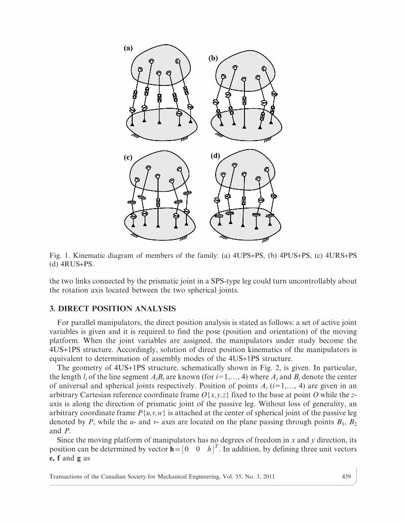
In our case, we selected a passive leg composed of two joints: a prismatic (P) joint and aspherical (S) one. As a consequence, the moving platform has four degrees of freedom and isconstrained to perform three rotations and one translation. If we apply four active legs and if itis assumed that each active leg has only two links and three joints then sum of degrees offreedom of the three joints is equal to six. By employing different joints in each leg, we can useprismatic (P), revolute (R), universal (U) and spherical (S) joints. Then, a family of parallelmanipulators (Fig. 1) is formed by the following architectures: 4UPS+PS, 4PUS+PS, 4URS+PSand 4RUS+PS. An underlined letter is an active joint which states the presence of an actuator.One can observe that all actuators are at or near the base. To decrease the reaction forces in thepassive prismatic joint, this joint can be replaced by a cylindrical one. Moreover, for mostkinematicians, substitution of universal joints for spherical ones is a common practice. Howeverfrom a technical point of view, this practice can produce undesirable situations. For example,


the two links connected by the prismatic joint in a SPS-type leg could turn uncontrollably aboutthe rotation axis located between the two spherical joints.

3. DIRECT POSITION ANALYSIS

For parallel manipulators, the direct position analysis is stated as follows: a set of active jointvariables is given and it is required to find the pose (position and orientation) of the movingplatform. When the joint variables are assigned, the manipulators under study become the4US+1PS structure. Accordingly, solution of direct position kinematics of the manipulators isequivalent to determination of assembly modes of the 4US+1PS structure.

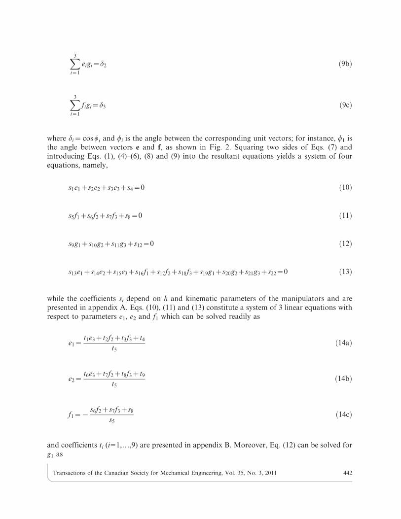
The geometry of 4US+1PS structure, schematically shown in Fig. 2, is given. In particular,the length li of the line segment AiBi are known (for i51,…, 4) where Ai and Bi denote the centerof universal and spherical joints respectively. Position of points Ai (i51,…, 4) are given in anarbitrary Cartesian reference coordinate frame O{x,y,z} fixed to the base at point O while the z-

axis is along the direction of prismatic joint of the passive leg. Without loss of generality, anarbitrary coordinate frame P{u,v,w} is attached at the center of spherical joint of the passive legdenoted by P, while the u- and v- axes are located on the plane passing through points B1, B2

and P.

Since the moving platform of manipulators has no degrees of freedom in x and y direction, itsposition can be determined by vector h~ 0 0 h½ �T . In addition, by defining three unit vectorse, f and g as

Fig. 1. Kinematic diagram of members of the family: (a) 4UPS+PS, (b) 4PUS+PS, (c) 4URS+PS(d) 4RUS+PS.


e~ e1 e2 e3½ �T~PB1��!PB1j j��! ð1aÞ

f~ f1 f2 f3½ �T~PB2��!PB2j j��! ð1bÞ

g~ g1 g2 g3½ �T~PB3��!PB3j j��! ð1cÞ

the orientation of moving platform can be obtained by a unit vector r as

r~ r1 r2 r3½ �T~e|f

e|fj j ð2Þ

while r is a unite vector along the w-axis and the sign ‘‘6’’ denotes the cross product betweenvectors. So the pose of moving platform (and the closure of the 4US+1PS structure) can beuniquely parameterized by seven parameters h, ei and fi (i51, 2, 3).

The closure equations for the structure are

aizlili~hzbi, i~1, . . . 4, ð3Þ

in which li is a unit vector representing the direction of vector AiBi��!

. Moreover, ai is the positionvector of the point Ai in the reference coordinate frame and is denoted as

Fig. 2. The 4US+1PS structure.


ai~OAi��!

~ ai1 ai2 ai3½ �T , i~1, . . . 4, ð4Þ

Taking into account Eqs. (1), vectors bi can be written accordingly as

b1~b1e ð5aÞ

b2~b2f ð5bÞ

b3~b3g ð5cÞ

where bi~PBi (for i51, 2, 3). Moreover, vector b4 can be defined as the linear combination ofthree other vectors b1, b2 and b3, as follows

b4~z1b1zz2b2zz3b3 ð6Þ

in which zi (i51, 2, 3) are three constant coefficients. Rearranging Eq. (3) yields

ai{h{bi~{lili, i~1, . . . 4, ð7Þ

Please note that the vectors e, f and g are unit vectors; thus

X3

i~1

e2i ~1 ð8aÞ

X3

i~1

f 2i ~1 ð8bÞ

X3

i~1

g2i ~1 ð8cÞ

and

X3

i~1

eifi~d1 ð9aÞ


X3

i~1

eigi~d2 ð9bÞ

X3

i~1

figi~d3 ð9cÞ

where di~ cos wi and wi is the angle between the corresponding unit vectors; for instance, w1 isthe angle between vectors e and f, as shown in Fig. 2. Squaring two sides of Eqs. (7) andintroducing Eqs. (1), (4)–(6), (8) and (9) into the resultant equations yields a system of fourequations, namely,

s1e1zs2e2zs3e3zs4~0 ð10Þ

s5f1zs6f2zs7f3zs8~0 ð11Þ

s9g1zs10g2zs11g3zs12~0 ð12Þ

s13e1zs14e2zs15e3zs16f1zs17f2zs18f3zs19g1zs20g2zs21g3zs22~0 ð13Þ

while the coefficients si depend on h and kinematic parameters of the manipulators and arepresented in appendix A. Eqs. (10), (11) and (13) constitute a system of 3 linear equations withrespect to parameters e1, e2 and f1 which can be solved readily as

e1~t1e3zt2f2zt3f3zt4

t5ð14aÞ

e2~t6e3zt7f2zt8f3zt9

t5ð14bÞ

f1~{s6f2zs7f3zs8

s5ð14cÞ

and coefficients ti (i51,…,9) are presented in appendix B. Moreover, Eq. (12) can be solved forg1 as


g1~{s10g2zs11g3zs12

s9ð15Þ

Now, introducing the above values of parameters e1, e2, f1 and g1 into Eqs. (8) and (9) leads to

u1e23zu2f 2

2 zu3f 23 zu4e3f2zu5e3f3zu6f2f3zu7e3zu8f2zu9f3zu10~0 ð16aÞ

u11f 22 zu12f 2

3 zu13f2f3zu14f2zu15f3zu16~0 ð16bÞ

u17f 22 zu18f 2

3 zu19e3f2zu20e3f3zu21f2f3zu22e3zu23f2zu24f3zu25~0 ð16cÞ

u26e3zu27f2zu28f3zu29~0 ð16dÞ

u30f2zu31f3zu32~0 ð16eÞ

and

G1g22zG2g2zG3~0 ð17Þ

where coefficients ui and Gi are presented in appendix C. Considering the values of coefficientssi, ti, ui and Gi, one can see that Eqs. (16) (17) are, in fact, a system of six nonlinear equations insix parameters h, e3, f2, f3, g2 and g3.

Variables f2 and f3 can be obtained from Eqs. (16d) and (16e), in terms of e3, as follows

f2~v1e3zv2

v3ð18Þ

f3~v4e3zv5

v3ð19Þ

while coefficients vi (i51,…, 5) are listed in appendix D. Substituting the values of parameters f2

and f3 from Eqs. (18) and (19) into Eqs. (16a) – (16c) and rearranging the resultant equationsyields a system of three nonlinear equations as

w1e23zw2e3zw3~0 ð20Þ




and coefficients wi (i51,…, 9) are presented in appendix D. Taking (20)6w42(21)6w1 and(20)6w72(22)6w1 respectively and rearranging the resultant equations leads to

m1e3zm2~0 ð23Þ

m3e3zm4~0 ð24Þ

where coefficients mi (i51,…, 4) are also listed in appendix D. Obtaining the parameter e3 fromEqs. (23) results in

e3~{m2

m1ð25Þ

Taking into account the values of parameters wi and mi, if Eq. (25) is introduced into Eqs.(20) and (24) then the following system of equations is obtained

H1g42zH2g3

2zH3g22zH4g2zH5~0 ð26Þ

H6g22zH7g2zH8~0 ð27Þ

where coefficients Hi (i51,…, 8) are polynomials of at most degree four in g3. Now, Eqs. (17),(26) and (27) constitute a system of three nonlinear equations with respect to parameters g2, g3

and h.

Parameter g2 can be eliminated from Eqs. (17) and (26) and form Eqs. (17) and (27) usingSylvester dialytic elimination method [21], see appendices E and F. The resultant equations arerespectively:

X16

i~0

Migi3~0 ð28Þ

and

X4

i~0

Nigi3~0 ð29Þ

where coefficients Mi and Ni are polynomials of at most degree four in h. Finally, variable g3

can be eliminated from Eqs.(28) and (29) again by Sylvester dialytic elimination method. Thisleads to a thirty -order polynomial in the unknown h as follows


X30

i~0

Rihi~0 ð30Þ

where Ri depends only on kinematic parameters of the manipulators. The detailed expressionsfor Ri are not given here because they are too large to serve any useful purpose. What isimportant to point out here is that the above equation admits at most thirty six solutions for h

while some of them may be complex.

Once h is found, the value(s) of g3 can be calculated from Eqs. (28) and (29) by setting thegreatest common divisor of these equations to be zero, In addition, the unique value of theother variables of vectors e, f, g and r can be calculated from Eqs. (1), (25), (18), (19), (14) and(15). Please note that only the solutions are admissible for which Eqs. (8) and (9) are satisfied.

With regard to the polynomials of Eqs. (28–30), one can conclude that there may bemore than 30 assembly configurations for a general member of this family of 3R1T parallelmanipulators. However, the following section will show that these polynomials will besummarized to a minimal univariate polynomial of degree 12 for a special architecture of themanipulators of this class.

4. A SPECIAL ARCHITECTURE OF THE MANIPULATORS

Consider a case in which vectors PB1��!

and PB2��!

are collinear with vectors PB3��!

and PB4��!

respectively, so the moving platform becomes planar. Moreover, it is assumed that actuators areuniformly and symmetrically distributed around the passive leg and the first actuator is locatedon the xz-plane. Thus, in this case, we have

g~{e ð31aÞ

z1~z3~0 ð31bÞ

a12~a21~a32~a41~0 ð31cÞ

With the above conditions, the coefficients si i[ {2, 5, 10, 13, 14, 15, 16, 19, 20, 21} becomezero in Eqs. (10–13). Therefore, these equations will change to

s1e1zs3e3zs4~0 ð32aÞ

s6f2zs7f3zs8~0 ð32bÞ

s9e1zs11e3{s12~0 ð32cÞ


s17f2zs18f3zs22~0 ð32dÞ

Equations (32) constitute two systems of linear equations with respect to parameters (e1, e3)and (f2, f3) respectively which can be solved as

e1~p1

p3, e3~

p2

p3, ð33aÞ

f2~p4

p6, f3~

p5

p6, ð33bÞ

where coefficients pi (i51,…, 6) are listed in appendix G. Introducing Eqs. (33) into Eqs. (8a),(8b) and (9a) results in

q1e22zq2~0 ð34aÞ

q3f 21 zq4~0 ð34bÞ

q5e2zq6f1zq7~0 ð34cÞ

and coefficients qi (i51,…, 7) are listed in appendix H. Now, Eqs. (34) constitute a system ofthree nonlinear equations in three unknowns e2, f1 and h. Introducing Eqs. (34b) and (34c) intoEq. (34a) yields a linear polynomial in f1 as follows

2q1q3q6q7f1{q1q4q26zq1q3q2

7zq2q25q3~0 ð35Þ

therefore

f1~q8

q9ð36Þ

where

q8~q1q4q26{q1q3q2

7{q2q25q3

q9~2q1q3q6q7

Now, the above value of f1 is substituted into Eq. (34b) which gives

q3q28zq4q2

9~0 ð37Þ


Expanding Eq. (37) leads to a twelfth-degree polynomial in h as

X12

i~0

Rihi~0 ð38Þ

The degree of above polynomial is much less then the degree of polynomial of Eq. (30), whichis due to the special architecture of the manipulators. In the next example, it is shown that theabove polynomial is minimal.

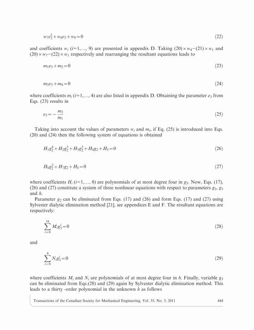
4.1. Numerical ExampleIn this example, the above presented method is applied to analyze the direct position

kinematics of a 4RUS+1PS parallel manipulator meeting conditions (31). The schematic modelof the manipulator is shown in Fig. 3.

For this manipulator, it is assumed that spherical joints of the active legs are located on acircle. Thus

b1~b2~b3~b ð39Þ

where b is the radius of the moving platform circle. Moreover, it is assumed that the revoluteactuators are on a circle too. Therefore, vectors ai can be computed from the followingrelations.

a1~ azd1 cos h1 0 d1 sin h1½ �T , a2~ 0 azd2 cos h2 d2 sin h2½ �T

a3~ {azd3 cos h3 0 d3 sin h3½ �T , a4~ 0 {azd4 cos h3 d4 sin h4½ �Tð40Þ

where di is equal to CiAi and a is the radius of base circle. hi is the rotation angle of the i-threvolute actuator with respect to xy plane and is considered positive when counterclockwise.Now the direct position kinematics of the manipulator is solved with the followings values:

a548 cm, b540 cm, d15d25d35d4555 cm, l1590 cm, l2585 cm, l35105 cm, l45105 cm,w1575u, h15h2565u, h35h45115u.

Fig. 3. The schematic model of a 4RUS+1PS parallel manipulator.


After calculating the parameters qi and introducing them into Eq. (37), the coefficients Ri arecalculated that are listed in Table 1. Now solving Eq. (38) yields twelve real solutions for h. Foreach value of h, the unique value of parameters ei, fi and consequently ri (i51, 2, 3) are obtainedfrom Eqs. (33), (36), (34c) and (2). This leads to twelve real solutions for the direct positionkinematics of the 4RUS+1PS manipulator that are presented in Table 2. Therefore, theunivariate polynomial of Eq. (38) is minimal. The graphical representation of the solutions isalso presented in Fig. 4. These solutions are correspondent to assembly modes of themanipulator.

In the next sections, direct velocity and direct kinematic singularities of the manipulatorsunder study are analyzed. First, direct Jacobian matrix of the manipulators is obtained.However, for the sake of brevity, one of the manipulators of this family, the 4-RUS+1PS, isselected for this aim.

5. DIRECT JACOBIAN MATRIX

Differentiating both sides of Eq. (3) with respect to time yields

_aaizlivi|li~vzv|bi ð41Þ

in which v~½ vx vy vz �T and v~½vx vy vz �T represent the three-dimensional linear andangular velocity of the moving platform, respectively. Moreover, vi represents the three-dimensional angular velocity of link AiBi (Fig. 5). For the 4-RUS+1PS parallel manipulator, thevector _aai can be written as

_aai~(ni|di) _hhi ð42Þ

where ni represents a unit vector along the axis of i-th revolute actuator, _hhi denotes the rate ofthis actuator and di is equal to vector CiAi

��!(Fig. 5). Introducing Eq. (42) into Eq. (41) results in

(ni|di) _hhizlivi|li~vzv|bi ð43Þ

The passive variables vi can be eliminated by dot multiplying both sides of Eq. (43) with li,which gives

Table 1. Coefficients Ri (i50,…, 12) obtained for the case study.

Coefficient value Coefficient value

R12 3.86878 R5 28555.456361010

R11 –2314.109686 R4 –42260.457661011

R10 564524.4070 R3 91230.872661010

R9 –70571452.93 R2 25120.621061013

R8 4476345931 R1 –42925.920861013

R7 –91065.429926106 R0 –47748.941161013

R6 –47019.077606108


(ni|di):li _hhi~v:liz(v|bi):li ð44Þ

where ‘‘?’’ denotes the dot product between vectors. Making use of formulae a:b~b:a anda:(b|c)~b:(c|a)~c:(a|b), Eq. (44) can be rewritten as

(ni|di):li _hhi~li:vz(bi|li):v ð45Þ

Let:x~ vT vT� �T

and _hh~ _hh1_hh2

_hh3_hh4

� �Tbe the vectors of the moving platform

velocities and the actuated joint rates, respectively. Then, Eq. (45) can be written in the matrixform as

Jq_hh~Jx

:x ð46Þ

where

Jq~

(n1|d1):l1 0 0 0

0 (n2|d2):l2 0 0

0 0 (n3|d3):l3 0

0 0 0 (n4|d4):l4

26664

37775

4|4

ð47Þ

Jx~

lT1 (b1|l1)T

lT2 (b2|l2)T

lT3 (b3|l3)T

lT4 (b4|l4)T

26664

37775

4|6

ð48Þ

Table 2. Solutions for the direct position kinematics of the manipulator.

No. h (cm) (r1, r2, r3)

1 80.2703 (–0.02781, –0.64099, 0.76704)2 87.7983 (0.43036, –0.56197, 0.70638)3 97.0392 (–0.50257, 0.26763, 0.82207)4 100.4495 (0.44669, 0.28676, –0.84749)5 106.5328 (–0.37533, –0.28944, –0.88054)6 137.5899 (0.04949, 0.30219, 0.95196)7 19.420 (0.73964, 0.26230, 0.61978)8 2.660 (0.50257, –0.26762, 0.82207)9 11.890 (–0.43036, 0.56197, 0.70638)10 –0.770 (–0.44669, –0.28676, –0.84749)11 –6.8399 (0.37533, 0.28944, –0.88054)12 –37.8899 (–0.04949, –0.30219, 0.95196)


Fig. 4. Twelve solutions of the direct kinematics problem corresponding to assembly modes of the4RUS+1PS manipulator.


are the inverse and direct Jacobian matrices of the 4-RUS+1PS manipulator respectively. If wedefine ti~bi|li, (i51,…, 4) then matrix Jx can be written in compact form as follows

Jx~

lT1 tT1

lT2 tT2

lT3 tT3

lT4 tT4

26664

37775

4|6

ð49Þ

Applying the above procedure for other manipulators under study, one can conclude thatEq. (49) presents the direct Jacobian matrix of all of these manipulators. However,the inverse Jacobian matrices are different and depend on the types of the legs of themanipulators.

6. DIRECT VELOCITY ANALYSIS

The objective of direct velocity analysis is to determine the velocity of the moving platformfrom a given set of velocities of the actuators in a given pose.

It is obvious that, due to the constraining passive leg of the presented manipulators, we havevx~vy~0; so the vector of moving platform velocity will be:

:x~½ 0 0 vz vx vy vz �T ð50Þ

which can be written in compact form as

:xc~½ vz vx vy vz �T ð51Þ

Considering the above discussion, one can see that arrays of the first and second columns ofJx does not effect on the instantaneous kinematics of the manipulator, so these arrays can be

Fig. 5. Sketch of a typical leg of the 4-RUS+1PS parallel manipulator.


eliminated and a new 464 direct Jacobian matrix is obtained as follows

Jc~

l1z tT1

l2z tT2

l3z tT3

l4z tT4

26664

37775

4|4

ð52Þ

where liz is the z component of vector li. When Jc is invertible, Eq. (46) can be written as

:xc~J{1

c Jq_hh ð53Þ

Equation (53) represents the direct velocity analysis of the parallel manipulators under study.

7. DIRECT KINEMATIC SINGULARITIES

A parallel manipulator gains extra degree(s) of freedom at direct kinematic singularities, evenif all actuators are locked, and becomes difficult to control at such configurations. So theseconfigurations should be found and avoided during the design and control stages of themanipulator. Numerous researchers have investigated singularity problems of parallelmanipulators; see for instance [22–24]. In this section, direct kinematic singularities of theproposed 4-DOF parallel manipulators are identified based on rank deficiency of the directJacobian matrix Jc presented in Eq. (52). Since the matrix Jc is a square matrix, the directkinematic singularities of the manipulators occur when det (Jc)50. Regarding Eq. (52), sevencases can be identified for the direct kinematic singularities.

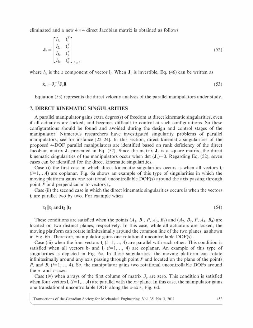
Case (i) the first case in which direct kinematic singularities occurs is when all vectors ti

(i51,…4) are coplanar. Fig. 6a shows an example of this type of singularities in which themoving platform gains one rotational uncontrollable DOF(s) around the axis passing throughpoint P and perpendicular to vectors ti.

Case (ii) the second case in which the direct kinematic singularities occurs is when the vectorsti are parallel two by two. For example when

t1jjt3 and t2jjt4 ð54Þ

These conditions are satisfied when the points (A1, B1, P, A3, B3) and (A2, B2, P, A4, B4) arelocated on two distinct planes, respectively. In this case, while all actuators are locked, themoving platform can rotate infinitesimally around the common line of the two planes, as shownin Fig. 6b. Therefore, manipulator gains one rotational uncontrollable DOF(s).

Case (iii) when the four vectors ti (i51,…, 4) are parallel with each other. This condition issatisfied when all vectors bi and li (i51,…, 4) are coplanar. An example of this type ofsingularities is depicted in Fig. 6c. In these singularities, the moving platform can rotateinfinitesimally around any axis passing through point P and located on the plane of the pointsP, and Bi (i51,…, 4). So, the manipulator gains two rotational uncontrollable DOFs aroundthe u- and v- axes.

Case (iv) when arrays of the first column of matrix Jc are zero. This condition is satisfiedwhen four vectors li (i51,…,4) are parallel with the xy plane. In this case, the manipulator gainsone translational uncontrollable DOF along the z-axis, Fig. 6d.


Case (v) when the arrays of one of the other columns (rather than the first column) of matrixJc are zero. This case is an special instance of case (i) in which vectors ti (i51,…,4) are coplanarand linearly dependent.

Case (vi) when the arrays of two columns (rather than the first column) of matrix Jc are zero.This case is an special instance of case (iii) in which vectors ti (i51,…,4) are parallel and linearlydependent.

Case (vii) when four vectors ti (i51,…, 4) are zero, i.e., when vectors bi and li are collinearwith each other for i51,…, 4, as shown in Fig. 6e. In this case, the moving platform can rotateinfinitesimally around any axis passing through point P, so the manipulator obtains threerotational uncontrollable DOFs around the u-, v- and w- axes.

8. CONCLUSION

A new family of 4-DOF 3R1T parallel manipulators with a passive constraining leg waspresented which can be used for flight simulation. The paper describes topology generation

Fig. 6. Five cases of direct kinematic singularities of the manipulators: (a) when vectors ti arecoplanar, (b) when vectors ti are parallel two by two, (c) when vectors ti are parallel with each other,(d) when vectors li (i51,…,4) are parallel with the xy plane and (e) when vectors ti are zero.


process and shows four alternative structures depending on the forms of actuation. Usingthree unit vectors, the echelon form direct position analysis of the manipulators wasperformed. The analysis provides a univariate polynomial of degree 30 together with a set oftwo other univariate polynomials. A special case was also reported in which it is shown thatthe number and degrees of these polynomials seriously depend on architectures and they canreduce to a univariate polynomial of degree 12 for a special architecture of the manipulators.A numerical example was also included to show that the latter polynomial is minimal. Next,direct velocity of the manipulators was analyzed using Jacobian matrices. Finally, directkinematic singularities were identified based on rank deficiently of the direct Jacobianmatrix.

REFERENCES

1. Gough, V.E. and Whitehall, S.G., ‘‘Universal tyre test machine,’’ 9th International Technical

Congress, FISITA, pp. 117–137, 1962.

2. Stewart, D.A., ‘‘Platform with six degrees of freedom,’’ Proceedings of the Institute of

Mechanical Engineering, Vol. 180, No. 5, pp. 371–386, 1965.

3. Clavel, R., ‘‘DELTA, A fast robot with parallel geometry,’’ Proceedings of 18th international

symposium on industrial robots, Lausanne, pp. 91–100, 1988.

4. Di Gregorio, R. and Parenti-Castelli, V., ‘‘A translational 3-DOF parallel manipulator,’’ In:

Lenarcic, J., Husty, M.L. editors. Advances in robot kinematics:analysis and control, Dordrecht:

Kluwer Academic Publishers, pp. 49–58, 1998.

5. Chablat, D. and Wenger, P., ‘‘Architecture optimization of a 3-DOF translational parallel

mechanism for machining applications, the Orthoglide,’’ IEEE Transactions on Robotics and

Automation, Vol. 19, No. 3, pp. 403–410, 2003.

6. Gallardo-Alvarado, J., Rico-Martınez, J.M., Alici, G.. ‘‘Kinematics and singularity analyses of

a 4-dof parallel manipulator using screw theory,’’ Mechanism and Machine Theory, Vol. 41, No.

9, pp. 1048–1061, 2006.

7. Bing, L. and Xiaojun, Y., Ying, H., ‘‘Kinematics analysis of a novel parallel platform with

passive constraint chain,’’ International Journal of Design Engineering, Vol. 1, No. 3, pp. 316–

332, 2009.

8. Chen, W.J., ‘‘A novel 4-dof parallel manipulator and its kinematic modeling,’’ IEEE

International Conference on Robotics and Automation, Seoul, May, pp. 3350–3355, 2001.

9. Gosselin, C.M. and Angeles, J., ‘‘The optimum kinematic design of a spherical three-degree-of-

freedom parallel manipulator,’’ ASME Journal of mechanisms, transmissions and automation in

design, Vol. 111, No. 2, pp. 202–207, 1989.

10. Huang, T., Gosselin, C.M., Whitehouse, D.J., Chetwynd, D.G., ‘‘Analytical approach for

optimal design of a type of spherical parallel manipulator using dexterous performance indices,’’

Proceedings of the Institute of Mechanical Engineering, Part C: J. Mechanical Engineering

Science, Vol. 217, pp. 447–455, 2003.

11. Pouliot, N., Gosselin, C.M., Nahon, M., ‘‘Motion simulation capabilities of three-degree-of-

freedom flight simulators,’’ AIAA Journal of Aircraft, Vol. 35, No. 1, 9–17, 1998.

12. Koevermans, W.P. et al., ‘‘Design and performance of the four d.o.f. motion system of the NLR

research flight simulator,’’ In AGARD Conference Proceeding, No 198, Flight Simulation, La

Haye, pp. 17–1/17–11, 1975.

13. Zlatanov, D. and Gosselin, C.M., ‘‘A family of new parallel architectures with four degrees offreedom,’’ EJCK, 1 (1), paper 6, 2002.


14. Zoppi, M., Zlatanov, D., Gosselin, C.M., ‘‘Analytical kinematics models and special geometries

of a class of 4-DOF parallel mechanisms,’’ IEEE Transactions on Robotics, Vol. 21, No. 6,

pp. 1046–1055, 2005.

15. Kong, X. and Gosselin, C. M., ‘‘Type synthesis of 4-DOF SP-equivalent parallel manipulators:

A virtual chain approach,’’ Mechanism and Machine Theory, Vol. 41, No. 11, pp. 1306–1319,

2006.

16. Herve, J. M., ‘‘Analyse structurelle des mecanismes par groupe des deplacements,’’ Mechanism

and Machine Theory, Vol. 13, pp. 437–450, 1978.

17. Fang, Y. and Tsai, L.-W., ‘‘Structure synthesis of a class of 4-DoF and 5-DoF parallel

manipulators with identical limb structures,’’ The International Journal of Robotics Research,

Vol. 21, No. 9, pp. 799–810, 2002.

18. Kong, X. and Gosselin, C.M., ‘‘Type synthesis of Three-degree-of-freedom spherical parallel

manipulators,’’ The International Journal of Robotics Research, Vol. 23, No. 3, pp. 237–245,

2004.

19. Carricato, M. and Parenti-Castelli, V., ‘‘A family of 3-DOF translational parallel

Manipulators,’’ ASME Journal of Mechanical Design, Vol. 125, No. 2, pp. 302–307, 2003.

20. Brogardh, T., ‘‘PKM Research - Important Issues, as seen from a Product Development

Perspective at ABB Robotics,’’ In Proceedings of the WORKSHOP on ‘‘Fundamental Issues and

Future Research Directions for Parallel Mechanisms and Manipulators’’ October 3–4, Quebec,

Canada, pp. 68–82, 2002.

21. Salmon, D. D., G., Lessons introductory to the modern higher algebra, third edition, Adamant

Media Corporation, 2002.

22. Gosselin, C. M. and Angeles, J., ‘‘Singularity analysis of closed-loop kinematic chains,’’ IEEE

Transactions on Robotics and Automation, Vol. 6, No. 3, pp. 281–90, 1990.

23. Zlatanov, D., Fenton, R.G., Benhabib, B., ‘‘Singularity Analysis of Mechanisms and Robots

Via a Velocity-Equation Model of The Instantaneous Kinematics,’’ Proceedings of IEEE

international conference on robotics and automation, San Diego, USA,Vol. 2, pp. 986 –991, 1994.

24. Zhao, J-S, Feng, Z-J, Zhou, K., Dong, J-X, ‘‘Analysis of the singularity of spatial parallel

manipulator with terminal constraints,’’ Mechanism and Machine Theory, Vol. 40, No. 3, pp. 275

–284, 2005.

APPENDIX A

Coefficients si are defined as

s1~{2a11b1, s2~{2a12b1, s3~(2h{2a13)b1, s4~b21za2

12za211za2

13{2ha13{l21zh2

s5~{2a21b2, s6~{2a22b2, s7~(2h{2a23)b2, s8~b22za2

22za221za2

23{2ha23{l22zh2,

s9~{2a31b3, s10~{2a32b3, s11~(2h{2a33)b3, s12~b23{2ha33za2

32za231za2

33{l23zh2,

s13~{2z1a41b1

s15~2z1b1h{2z1b1a43, s16~{2z2a41b2, s17~{2z2a42b2

s18~2z2b2h{2z2a43b2, s19~{2z3a41b3, s20~{2z3a42b3, s21~2z3b3h{2z3a43b3

s22~h2{l24za2

41za242{2ha43za2

43zz21b2

1zz22b2

2zz23b2

3z

2b1b3z1z3d2z2b2b3z2z3d3z2b1b2z1z2d1


APPENDIX B

Coefficients ti are

t1~{s2s15s5s9zs3s5s9s14, t2~s2s16s9s6{s2s17s5s9, t3~s2s16s9s7{s2s18s5s9

t4~({s2s20s5s9zs2s19s5s10)g2z(s2s19s5s11{s2s21s5s9)g3z

s4s5s9s14zs2s16s9s8{s2s22s5s9zs2s19s5s12

t5~s5s9(s13s2{s14s1), t6~{s13s5s9s3zs15s1s5s9, t7~s17s1s5s9{s16s1s9s6

t8~{s16s1s9s7zs18s1s5s9

t9~({s19s1s5s10zs20s1s5s9)g2z(s21s1s5s9{s19s1s5s11)g3z

s22s1s5s9{s13s5s9s4{s16s1s9s8{s19s1s5s12

APPENDIX C

Coefficients ui and Gi are as follows

u1~t26zt2

5zt21, u2~t2

7zt22, u3~t2

3zt28, u4~2t1t2z2t6t7, u5~2t6t8z2t1t3

u6~2t7t8z2t2t3, u7~2t6t9z2t1t4, u8~2t7t9z2t2t4, u9~2t8t9z2t3t4,

u10~{t25zt2

9zt24, u11~s2

5zs26, u12~s2

7zs25,u13~2s6s7, u14~2s6s8

u15~2s7s8, u16~{s25zs2

8, u17~{t2s6zs5t7, u18~{t3s7, u19~s5t6{t1s6

u20~{t1s7zt5s5, u21~s5t8{t2s7{t3s6, u22~{t1s8

u23~{t4s6{t2s8zs5t9, u24~{t3s8{t4s7, u25~{t4s8{d1t5s5

u26~({t1s10zs9t6)g2z(t5s9{t1s11)g3{t1s12, u27~({t2s10zs9t7)g2{t2s11g3{t2s12


u28~(s9t8{t3s10)g2{t3s11g3{t3s12, u29~({t4s10zs9t9)g2{t4s11g3{d2t5s9{t4s12

u30~(s6s10zs9s5)g2zs6s11g3zs6s12, u31~s7s10g2z(s7s11zs9s5)g3zs7s12

u32~s8s10g2zs8s11g3{d3s9s5zs8s12

G1~s29zs2

10, G2~2(s10s12zs10s11g3), G3~(s211zs2

9)g23z2s11s12g3{s2

9zs212

APPENDIX D

Coefficients vi, wi and mi are as follows

v1~{u26u31, v2~u28u32{u29u31, v3~{u30u28zu31u27, v4~u30u26, v5~u30u29{u32u27

w1~u5v3v4zu1v23zu3v2

4zu2v21zu6v1v4zu4v3v1

w2~u6v2v4z2u3v4v5z2u2v1v2zu4v3v2zu5v3v5zu6v1v5zu9v3v4zu7v23zu8v3v1

w3~u8v3v2zu6v2v5zu3v25zu2v2

2zu10v23zu9v3v5

w4~u11v21zu12v2

4zu13v1v4

w5~2u12v4v5zu14v3v1zu13v1v5zu13v2v4z2u11v1v2zu15v3v4


2zu14v3v2zu12v25zu13v2v5

w7~u17v21zu18v2

4zu19v3v1zu20v3v4zu21v1v4

w8~2u18v4v5z2u17v1v2zu19v3v2zu21v2v4zu20v3v5zu21v1v5zu24v3v4zu22v23zu23v3v1



2zu23v3v2zu25v23zu24v3v5

m1~w2w4{w1w5, m2~w3w4{w1w6, m3~w2w7{w1w8, m4~w3w7{w1w9

APPENDIX E

The term g42 can be eliminated from Eqs. (17) and (26) through multiplying them by H1g2

2 andG1 respectively. Subtraction of the obtained expressions results in

(G1H2{G2H1)g32z(G1H3{G3H1)g2

2zG1H4g2zG1H5~0 ðE1Þ

The procedure is repeated by multiplying Eqs. (17) and (26) in (H1g2zH2)g22 and G1g2zG2

respectively. Subtraction of the obtained equations yields

(G1H3{G3H1)g32z(G1H4zG2H3{G3H2)g2

2z(G1H5zG2H4)g2zG2H5~0 ðE2Þ

In addition, multiplying Eq. (17) by g2 results in

G1g32zG2g2

2zG3g2~0 ðE3Þ

Eqs. (E1) 2(E3) and (17) can be written in a matrix form as

K1

g32

g22

g

1

26664

37775~

0

0

0

0

26664

37775 ðE4Þ

where

K1~

G1H2{G2H1 G1H3{G3H1 G1H4 G1H5

G1H3{G3H1 G1H4zG2H3{G3H2 G1H5zG2H4 G2H5

G1 G2 G3 0

0 G1 G2 G3

26664

37775

Eq. (E4) is valid if and only if det(K1)50. Equating determinant of K1 to zero leads to apolynomial of degree 16 as Eq. (28).


APPENDIX F

Taking (17)6H62(27)6G1 and (17)6H82(27)6G3 respectively and rewriting the resultantequations in matrix form, we have

K2

g2

1

� �~

0

0

� �ðF1Þ

where

K2~G2H6{G1H7 G3H6{G1H8

G1H8{G3H6 G2H8{G3H7

� �

Again, Eq. (F1) is valid if and only if det(K2)50. Thus

(G2H6{G1H7)(G2H8{G3H7)z(G3H6{G1H8)2~0 ðF2Þ

Now, taking into account the values of parameters Hi and Gi, Eq. (F2) can be written as Eq.(29).

APPENDIX G

Coefficients pi are as follows

p1~s3s12zs4s11, p2~{s4s9{s1s12, p3~s3s9{s1s11,

p4~s7s22{s8s18, p5~s8s17{s6s22, p6~s6s18{s7s17

APPENDIX H

Coefficients qi are

q1~p23, q2~p2

1zp22{p2

3, q3~p26, q4~p2

4zp25{p2

6, q5~p3p4, q6~p1p6, q7~p2p5{p33p6


Direct kinematic analysis of a family of 4-DOF parallel manipulators

Documents

Transcript of Direct kinematic analysis of a family of 4-DOF parallel manipulators