Dipòsit Digital de Documents de la UAB...the Forest Sciences Centre of Catalonia, the University of...
327
Transcript of Dipòsit Digital de Documents de la UAB...the Forest Sciences Centre of Catalonia, the University of...

2013, Cover drawing by Helena Marcer i Espunya
A contribution to the use, modelling and
organization of data in biodiversity conservation
A PhD dissertation presented by
Arnald Marcer i Batlle
with the acceptance of the dissertation’ s supervisors:
Dr. Joan Pino Dr. Xavier Pons
CREAF, UAB UAB
CREAF, Universitat Autonoma de Barcelona
Cerdanyola del Valles
March 2013


Ai festa, petapigona!
Dedicated to Helena, Anna and my parents


Contents
Contents v
List of Figures ix
List of Tables xi
List of Acronyms xiii
Acknowledgements 3
1 Introduction 5
1.1 Setting the problem . . . . . . . . . . . . . . . . . . . . . . . . . . . . . . . 5
1.2 Biodiversity data . . . . . . . . . . . . . . . . . . . . . . . . . . . . . . . . 8
1.3 Mapping for biodiversity conservation . . . . . . . . . . . . . . . . . . . . . 14
1.4 Species distribution modelling . . . . . . . . . . . . . . . . . . . . . . . . . 18
1.5 Biodiversity Conservation Information Systems . . . . . . . . . . . . . . . 32
1.6 Dissertation structure . . . . . . . . . . . . . . . . . . . . . . . . . . . . . . 38
2 Modelling distributions for rare species conservation 41
2.1 Abstract . . . . . . . . . . . . . . . . . . . . . . . . . . . . . . . . . . . . . 42
2.2 Introduction . . . . . . . . . . . . . . . . . . . . . . . . . . . . . . . . . . . 43
2.3 Methods . . . . . . . . . . . . . . . . . . . . . . . . . . . . . . . . . . . . . 45
2.4 Results . . . . . . . . . . . . . . . . . . . . . . . . . . . . . . . . . . . . . . 53
2.5 Discussion . . . . . . . . . . . . . . . . . . . . . . . . . . . . . . . . . . . . 57
v

vi CONTENTS
2.6 Conclusions . . . . . . . . . . . . . . . . . . . . . . . . . . . . . . . . . . . 61
2.7 Acknowledgements . . . . . . . . . . . . . . . . . . . . . . . . . . . . . . . 62
3 Modelling IAS distributions from biodiversity atlases 63
3.1 Abstract . . . . . . . . . . . . . . . . . . . . . . . . . . . . . . . . . . . . . 64
3.2 Introduction . . . . . . . . . . . . . . . . . . . . . . . . . . . . . . . . . . . 65
3.3 Methods . . . . . . . . . . . . . . . . . . . . . . . . . . . . . . . . . . . . . 67
3.4 Results . . . . . . . . . . . . . . . . . . . . . . . . . . . . . . . . . . . . . . 76
3.5 Discussion . . . . . . . . . . . . . . . . . . . . . . . . . . . . . . . . . . . . 80
3.6 Conclusions . . . . . . . . . . . . . . . . . . . . . . . . . . . . . . . . . . . 82
3.7 Acknowledgements . . . . . . . . . . . . . . . . . . . . . . . . . . . . . . . 83
4 Protected Areas’ Information System 85
4.1 Abstract . . . . . . . . . . . . . . . . . . . . . . . . . . . . . . . . . . . . . 86
4.2 Introduction . . . . . . . . . . . . . . . . . . . . . . . . . . . . . . . . . . . 87
4.3 Legal context . . . . . . . . . . . . . . . . . . . . . . . . . . . . . . . . . . 91
4.4 System design and implementation . . . . . . . . . . . . . . . . . . . . . . 92
4.5 Discussion . . . . . . . . . . . . . . . . . . . . . . . . . . . . . . . . . . . . 101
4.6 Conclusions . . . . . . . . . . . . . . . . . . . . . . . . . . . . . . . . . . . 105
4.7 Acknowledgements . . . . . . . . . . . . . . . . . . . . . . . . . . . . . . . 106
5 General discussion and conclusions 107
5.1 General discussion . . . . . . . . . . . . . . . . . . . . . . . . . . . . . . . 107
5.2 Conclusions . . . . . . . . . . . . . . . . . . . . . . . . . . . . . . . . . . . 119
5.3 Further research . . . . . . . . . . . . . . . . . . . . . . . . . . . . . . . . . 122
References 123
Appendix A Distribution model maps of SCI 159
Appendix B Protected range maps of SCI 167
Appendix C Protected range sizes of SCI 175

CONTENTS vii
Appendix D Occurrence maps of IAS 305


List of Figures
1.1 Dimensions of biodiversity data . . . . . . . . . . . . . . . . . . . . . . . . . . 11
1.2 Myers' biodiversity hotspots . . . . . . . . . . . . . . . . . . . . . . . . . . . . 16
1.3 Ailanthus altissima world distribution . . . . . . . . . . . . . . . . . . . . . . 17
1.4 World Database on Protected Areas . . . . . . . . . . . . . . . . . . . . . . . . 17
1.5 Species Distribution Modelling methods . . . . . . . . . . . . . . . . . . . . . 23
2.1 SCI modelling study area . . . . . . . . . . . . . . . . . . . . . . . . . . . . . 46
2.2 SCI range maps . . . . . . . . . . . . . . . . . . . . . . . . . . . . . . . . . . . 56
2.3 SCI range maps . . . . . . . . . . . . . . . . . . . . . . . . . . . . . . . . . . . 57
3.1 IAS study area . . . . . . . . . . . . . . . . . . . . . . . . . . . . . . . . . . . 67
3.2 IAS modelling work ow methodology . . . . . . . . . . . . . . . . . . . . . . . 72
3.3 IAS maps of best models . . . . . . . . . . . . . . . . . . . . . . . . . . . . . . 78
3.4 IAS bad model examples . . . . . . . . . . . . . . . . . . . . . . . . . . . . . . 80
4.1 Natura 2000 designation process . . . . . . . . . . . . . . . . . . . . . . . . . . 92
4.2 General architecture of the protected areas' information system . . . . . . . . 94
4.3 Protected areas' system main model classes . . . . . . . . . . . . . . . . . . . 96
4.4 Protected Areas' Information System screenshots . . . . . . . . . . . . . . . . 99
4.5 Flow diagram for declaration of protected area . . . . . . . . . . . . . . . . . . 101
A.1 Distribution model of Asplenium majoricum Litard. . . . . . . . . . . . . . . . 160
A.2 Distribution model of Carduncellus dianius (Webb) G. L�opez . . . . . . . . . . 161
ix
x LIST OF FIGURES
A.3 Distribution model of Diplotaxis ibicensis (Pau) G�omez Campo . . . . . . . . 162
A.4 Distribution model of Euphorbia squamigera Loisel. . . . . . . . . . . . . . . . 163
A.5 Distribution model of Helianthemum caput-felis Boiss. . . . . . . . . . . . . . 164
A.6 Distribution model of Medicago citrina (Font Quer) Greuter . . . . . . . . . . 165
A.7 Distribution model of Silene hifacensis Rouy ex Willk. . . . . . . . . . . . . . 166
B.1 Asplenium majoricum protected range . . . . . . . . . . . . . . . . . . . . . . 168
B.2 Carduncellus dianius protected range . . . . . . . . . . . . . . . . . . . . . . . 169
B.3 Diplotaxis ibicensis protected range . . . . . . . . . . . . . . . . . . . . . . . . 170
B.4 Euphorbia squamigera protected range . . . . . . . . . . . . . . . . . . . . . . 171
B.5 Helianthemum caput-felis protected range . . . . . . . . . . . . . . . . . . . . 172
B.6 Medicago citrina protected range . . . . . . . . . . . . . . . . . . . . . . . . . 173
B.7 Silene hifacensis protected range . . . . . . . . . . . . . . . . . . . . . . . . . 174
D.1 Occurrences of Agave americana . . . . . . . . . . . . . . . . . . . . . . . . . 306
D.2 Occurrences of Ailanthus altissima . . . . . . . . . . . . . . . . . . . . . . . . 306
D.3 Occurrences of Conyza canadensis . . . . . . . . . . . . . . . . . . . . . . . . . 307
D.4 Occurrences of Datura stramonium . . . . . . . . . . . . . . . . . . . . . . . . 307
D.5 Occurrences of Oenothera biennis . . . . . . . . . . . . . . . . . . . . . . . . . 308
D.6 Occurrences of Opuntia ficus-indica . . . . . . . . . . . . . . . . . . . . . . . . 308
D.7 Occurrences of Oxalis pes-caprae . . . . . . . . . . . . . . . . . . . . . . . . . 309
D.8 Occurrences of Robinia pseudoacacia . . . . . . . . . . . . . . . . . . . . . . . 309
D.9 Occurrences of Xanthium spinosum . . . . . . . . . . . . . . . . . . . . . . . . 310
D.10 Occurrences of Amaranthus albus . . . . . . . . . . . . . . . . . . . . . . . . . 310
List of Tables
1.1 Threshold-dependent accuracy measures . . . . . . . . . . . . . . . . . . . . . 27
2.1 SCI occurrences . . . . . . . . . . . . . . . . . . . . . . . . . . . . . . . . . . . 47
2.2 SCI modelling environmental predictors . . . . . . . . . . . . . . . . . . . . . 49
2.3 SCI �nally chosen models . . . . . . . . . . . . . . . . . . . . . . . . . . . . . 54
2.4 SCI estimated ranges . . . . . . . . . . . . . . . . . . . . . . . . . . . . . . . . 55
2.5 SCI conservation status and protection . . . . . . . . . . . . . . . . . . . . . . 58
3.1 List of selected IAS for modelling . . . . . . . . . . . . . . . . . . . . . . . . . 69
3.2 IAS modelling predictors . . . . . . . . . . . . . . . . . . . . . . . . . . . . . . 71
3.3 IAS �nally accepted models . . . . . . . . . . . . . . . . . . . . . . . . . . . . 74
3.4 Summary of �nally accepted IAS models . . . . . . . . . . . . . . . . . . . . . 79
C.1 Asplenium majoricum PSA protection by Natura 2000 . . . . . . . . . . . . . 178
C.2 Asplenium majoricum EOO and AOO protection by Natura 2000 . . . . . . . 197
C.3 Asplenium majoricum PSA protection by North African protected areas . . . 200
C.4 Carduncellus dianius PSA protection by Natura 2000 . . . . . . . . . . . . . . 201
C.5 Carduncellus dianius EOO and AOO protection by Natura 2000 . . . . . . . . 211
C.6 Carduncellus dianius PSA protection by North African protected areas . . . . 212
C.7 Diplotaxis ibicensis PSA protection by Natura 2000 . . . . . . . . . . . . . . . 213
C.8 Diplotaxis ibicensis EOO and AOO protection by Natura 2000 . . . . . . . . . 221
C.9 Diplotaxis ibicensis PSA protection by North African protected areas . . . . . 224
xi

xii LIST OF TABLES
C.10 Euphoriba squamigera PSA protection by Natura 2000 . . . . . . . . . . . . . 225
C.11 Euphorbia squamigera EOO and AOO protection by Natura 2000 . . . . . . . 258
C.12 Euphorbia squamigera PSA protection by North African protected areas . . . 266
C.13 Euphorbia squamigera EOO and AOO protection by North African protected
areas . . . . . . . . . . . . . . . . . . . . . . . . . . . . . . . . . . . . . . . . . 271
C.14 Helianthemum caput-felis PSA protection by Natura 2000 . . . . . . . . . . . 274
C.15 Helianthemum caput-felis EOO and AOO protection by Natura 2000 . . . . . 288
C.16 Helianthemum caput-felis PSA protection by North African protected areas . . 291
C.17 Helianthemum caput-felis EOO and AOO protection by North African protected
areas . . . . . . . . . . . . . . . . . . . . . . . . . . . . . . . . . . . . . . . . . 293
C.18 Medicago citrina PSA protection by Natura 2000 . . . . . . . . . . . . . . . . 294
C.19 Medicago citrina EOO and AOO protection by Natura 2000 . . . . . . . . . . 297
C.20 Silene hifacensis PSA protection by Natura 2000 . . . . . . . . . . . . . . . . 298
C.21 Silene hifacensis EOO and AOO protection by Natura 2000 . . . . . . . . . . 302
C.22 Silene hifacensis PSA protection by North African protected areas . . . . . . . 303
List of Abbreviations
AJAX Asynchronous Javascript and XML
ANN Arti�cial Neural Networks
AUC Area Under the Curve
AOO Area of Occupancy
BAM Biotic, Abiotic and Movements diagram
BDBC Biodiversity Data Bank of Catalonia
BRT Boosted Regression Trees
BHL Biodiversity Heritage Library
CAPAD Collaborative Australian Protected Areas Database
CART Classi�cation and Regression Trees
CDDA European Common Database on Designated Areas
CSV Comma-Separated Values
DAISIE Delivering Alien Invasive Species Inventories for Europe (EU funded project)
DCAC Digital Climatic Atlas of Catalonia
ENFA Ecological Niche Factor Analysis
EOO Extent of Occurrence
EOL Encyclopedia of Life
EPSG European Petroleum Survey Group
ETRS89 European Terrestrial Reference System 1989
xiii
xiv LIST OF ABBREVIATIONS
FishNet Global Network of Ichtyology Collections
GADM Global ADMinistrative areas database
GAM Generalised Additive Models
GARP Genetic Algorithm for Rule-Set Production
GBIF Global Biodiversity Information Facility
GIS Geographical Information System
GLM Generalised Linear Models
GML Geography Markup Language
HerpNet Global Network of Herpetological Collections
IAS Invasive Alien Species
ICREA Instituci�o Catalana de Recerca i Estudis Avan�cats (Catalan Institution for Re-
search and Advanced Studies)
ICT Information and Communication Technologies
INSPIRE Infrastructure for Spatial Information in Europe
IUCN International Union for the Conservation of Nature
LAEA Lambert Azimuthal Equal Area
ManIS Mammal Networked Information System
MARS Multivariate Adaptive Regression Splines
MaxEnt Maximum Entropy
MPA Minimum Predicted Area
MTP Minimum Training Presence
OGC Open Geospatial Consortium
PAD-US Protected Areas Database of the United States
PSA Potentially Suitable Areas
ROC Receiver Operating Characteristic
SAC Spatial AutoCorrelation (in statistics modelling)

1
SAC Special Areas of Conservation (in European Legislation)
SCI Species of Conservation Interest (in Chapter 2)
SCI Sites of Community Importance (in European legislation)
SDM Species Distribution Modelling
SIPAN Sistema d'Informaci�o sobre el Patrimoni Natural de Catalunya (Natural Heritage
Information System of Catalonia)
SPA Special Protection Areas
SQL Structured Query Language
SVM Support Vector Machines
TOL Tree of Life
UNEP United Nations Environment Programme
UTM-ED50 Universal Transverse Mercator, European Datum 1950
VertNet Global Network of Vertebrate Species
WCMC World Conservation Monitoring Center
WDPA World Database on Protected Areas
WGS World Geodetic System
XML Extensible Markup Language
WMS Web Map Service

Acknowledgements
In the past 17 years I have been fortunate enough to work at an excellent, lively researchcentre that has provided a nurturing environment. I am grateful to the centre, personi�edin its three directors: Jaume Terrades, Ferran Rod�a and Javier Retana. Jaume o�eredme the opportunity to join CREAF, Ferran gave me his support and new responsibilitiesand Javi provided the institutional context in which this dissertation has been possible.Xavier Pons gave me the professional opportunity to work at CREAF in his dynamic andexcellent team at a crucial moment in my career.
I am very grateful to Joan Pino and Xavier Pons for accepting to supervise mydissertation and wisely guiding me along this process. Joan, thank you for your continuedwords of support during this process. Anna Espunya has revised the manuscript with akeen but loving eye for the details of academic writing.
Agust�� Escobar and V��ctor Garcia deserve a very special mention. Combining a PhDwith work would not have been possible without the dedication and brightfulness youalways put on our projects. Anna Grau has also been a �ne addition in the last months ofthis dissertation. It is a pleasure to work with you all.
Special thanks to all my friends, colleagues and collaborators, at CREAF and Grumets,the Catalan public environmental administration, the Natural History Museum of Barcelona,the Forest Sciences Centre of Catalonia, the University of Barcelona and the Do~nanaBiological Station with which it is a pleasure to work.
CREAF is a nice place to work at because of its people. I will not name you sinceforgetting anyone would be unjusti�ed. Thank you all for your day-to-day companionshipand friendliness.
Special thanks to my colleague and friend Jordi Vayreda with whom I shared longo�ce hours and the experience of carrying out a PhD. He always has words of support.And to Joanjo, a good friend who is also engaged on his own PhD endeavour. All mysupport.
Thanks to all my friends, those from whom time has physically separated me and thosewith whom I am still lucky enough to share experiences. It is a pleasure to share bicyclerides, crazy football polls, hiking, dinners and delightful get-togethers with all of you.
[Gracies a tots els meus amics, als que el temps me n’ha separat fısicament i als ambqui tinc la sort de compartir experiencies. Es un plaer compartir anades en bici, porres
3
4 LIST OF ABBREVIATIONS
boges de futbol, caminades, sopars i trobades amb tots vosaltres.]
And �nally, I thank my family for all their love and encouragement: my parents,without whom I wouldn't be here; Anna, my wife, for her unconditional support, a�ectionand love; and our daughter Helena, who �lls our life with joy and tremendous fun.
[I finalment, Voldria agrair a la meva famılia per tot el seu amor i suport: als meuspares, sense els quals jo no hauria arribat aquı; l’Anna, la meva dona, pel seu recolzament,afecte i amor incondicionals; i la nostra filla Helena, que omple la nostra vida de joia igran divertiment.]
This dissertation has partly been possible thanks to the support of project CONSOLIDER-
MONTES (CSD2008-00040) of the Ministerio de Ciencia e Innovaci�on of the Spanish
government and of the General Directorate of the Environment and Housing Department
of the Autonomous Government of Catalonia. I wish to thank also Llu��s Brotons, Arthur
Chapman, Robert Guralnick, Jane Elith and other anonymous reviewers for their comments
which very much helped in improving di�erent chapters.

Chapter 1
Introduction
Biological diversity must be treated more
seriously as a global resource, to be in-
dexed, used, and above all, preserved.
Three circumstances conspire to give this
matter an unprecedented urgency. First,
exploding human populations are degrad-
ing the environment at an accelerated rate,
especially in tropical countries. Second, science is discovering
new uses for biological diversity in ways that can relieve both hu-
man suffering and environmental destruction. Third, much of the
diversity is being irreversibly lost through extinction caused by
the destruction of natural habitats, again especially in the tropics.
Overall, we are locked into a race. We must hurry to acquire the
knowledge on which a wise policy of conservation and development
can be based for centuries to come.
E.O. Wilson, 1988
1.1 Setting the problem
If we are to preserve our threatened biodiversity we need to hurry to acquire the
knowledge on which a wise policy of conservation and development can be based for
5

6 CHAPTER 1. INTRODUCTION
centuries to come (Wilson, 1988). To succeed in such an endeavour, we �rst need data
and analytical tools to gain such knowledge and second, we need to be able to convey this
knowledge to the research and conservation management communities so that it can be
put to good use.
The knowledge of species' distributions is fundamental in conservation practice. Ideally,
in order to model the distribution of a given species, we would need a large, �ne-resolution,
unbiased set of presences and absences. In reality, we are often limited to sets of species'
occurrence data which are scarce, presence-only, biased, not extensive and at coarse
resolutions (Newbold, 2010; Niamir et al., 2011). Although the size of species occurrence
data as a whole can be huge (GBIF, 2013a), this is not so at the level of individual taxons
or species, and numerous references in the scienti�c literature point at that problem,
e.g. Guisan et al. (2006a); Pearson et al. (2007); Platts et al. (2010). Yet, The need for
information on the distribution of single species is of central importance to conserving
biodiversity (Robertson et al., 2010).
Our main asset to deal with this data conundrum is the wide range of analytical tools
we have at our disposal. Recent advances in statistics, computer science and information
technologies have allowed the emergence of the �eld of biodiversity informatics (Schnase
et al., 2003; Peterson et al., 2010) and its application to conservation planning and
management (Sober�on and Peterson, 2004). This can be used to tackle ”the unprecedented
urgency with which biodiversity needs to be indexed, used, and above all, preserved” ( Wilson
(1988), p.3). The increasing digital availability of biodiversity occurrence data (Yesson et al.,
2007; Anderson, 2012) and protected area boundaries (IUCN-UNEP, 2013) combined with
novel methods in species distribution modelling (Franklin, 2009; Peterson et al., 2011) can
greatly enhance the analysis of biodiversity conservation and help devise e�ective actions
aimed at its preservation and, hopefully, succeed in the true protection of our world's
natural heritage. A wide range of species distribution modelling methodologies are aimed
at dealing with the wide range of data situations, from presence-only to presence-absence
data (Franklin, 2009; Peterson et al., 2011). Yet, the challenge is enormous.

1.1. SETTING THE PROBLEM 7
Aim
This dissertation aims at making a contribution on methods for dealing with con-
straints in biodiversity data, speci�cally species occurrences, for producing maps useful
in conservation management and plannning using species distribution modelling as a
tool. It concentrates on the modelling of species of conservation interest and of alien
invasive species since they embody two complementary objectives: preserving values and
avoiding threats. The speci�c examples have been chosen because of the di�erent particular
modelling di�culties they pose: a) narrowly-distributed endemics with scarce but high
quality data and b) scarce, biased, �ne-resolution data of unknown quality but which have
an abundant, reliable, coarse-resolution data counterpart. This latter example deals also
with the equilibrium assumption problem inherent to modelling the distribution of invasive
species (V�aclav��k and Meentemeyer, 2012).
A design and implementation of an information system on protected areas which
bridges the analysis of spatial patterns of biodiversity, i.e. species distributions, with
its protection is also provided. Protected areas play a crucial role in the preservation of
biodiversity (Rodrigues et al., 2004b,a) and their coverage area is considered a surrogate
indicator of its protection (Chape et al., 2005; Jones et al., 2011). If we are to monitor
the progress of biodiversity protection over time, information systems are needed which
can deal with changes in protected area boundaries over time. This dissertation provides
a design and implementation of such an information system.
The aim of this dissertation is two-fold:
� To explore the use of scarce, problematic species occurrence data to derive information
which is useful in conservation planning and management and which can contribute
to the knowledge necessary to preserve the world's biodiversity.
� To use information systems technology as a tool to organize and convey information
on biodiversity protection which, in combination with species' distribution maps,
can help the research and conservation management communities and, ultimately,
society at large.

8 CHAPTER 1. INTRODUCTION
In this chapter I brie y frame the research in its broader scienti�c context. First, I
present the nature of biodiversity data at the species level and state the need to express
it in a spatial context. Second, I outline the role of species distribution modelling in
providing distribution or range maps. Finally, I argue for the use of information systems
for biodiversity conservation, centered on protected areas.
1.2 Biodiversity data
The term biodiversity refers to the diversity or variation in biological entities or life
itself, at all levels, from genes to biomes, as well as the ecological and evolutionary processes
that give birth to and maintain it. As the Convention on Biological Diversity (United
Nations Environmental Programmme (UNEP), 1992) de�nes it as follows: Biological
diversity means the variability among living organisms from all sources including, inter
alia, terrestrial, marine and other aquatic ecosystems and the ecological complexes of which
they are part: this includes diversity within species, between species and of ecosystems.
The focus of this dissertation is on using primary data to obtain secondary or derived data
which can be useful in the conservation of biodiversity (see Box 1). The quantity and
quality of species distributional data can profoundly in uence the quality of products that
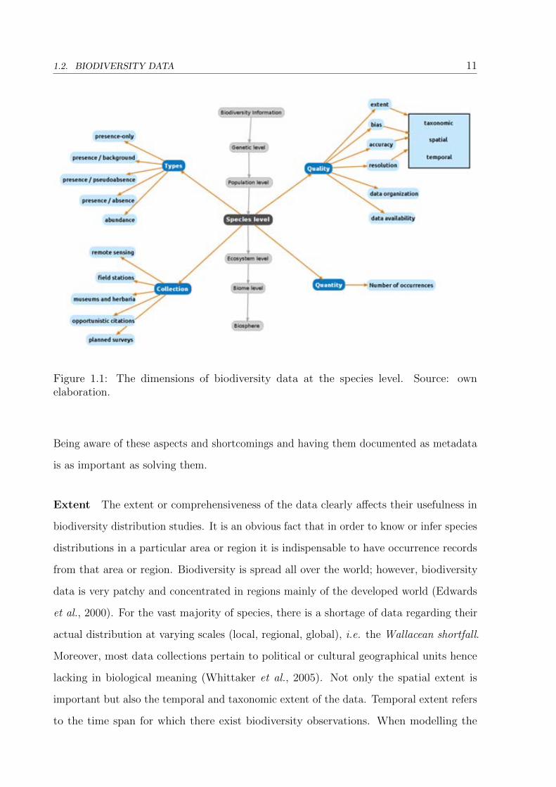
are then used to direct (or misdirect) conservation action (Robertson et al., 2010). Figure
1.1 provides a general overview of biodiversity data. Among all of their levels, from the
genes to the Biosphere, this dissertation is centered at the species data level. At this level,
I will analyse the quantity and quality dimensions of data and how the di�erent types of
data require di�erent modelling approaches. Data collection is beyond the scope of this
dissertation, it will only be mentioned indirectly.
In this section we will take a broad view of two of the dimensions of biodiversity data:
quantity and quality.
Quantity of biodiversity data. Data scarcity or data deluge
There is a wealth of data which have been recorded over the centuries in an ad hoc way
by natural historians, museums, scientists and the like in the form of museum specimens,

1.2. BIODIVERSITY DATA 9
site inventories, citations in technical and scienti�c literature, etc. (Chapman and Busby,
1994; Chapman et al., 2005). Over the last two decades these data have been translated into
digital repositories by both governmental and non-governmental organizations, investing
considerable amounts of �nancial resources (Robertson et al., 2010). These databases
represent an invaluable and still largely untapped potential asset of data for science
and conservation (Funk and Richardson, 2002; Graham et al., 2004; Suarez and Tsutsui,
2004; Guisan et al., 2006b; Franklin, 2009; Robertson et al., 2010). GBIF, the Global
Biodiversity Information Facility, which collates data from digital databases around the
world, exempli�es the size of existing data. Currently (as of 3 January 2012), it contains
over 380 million data records coming from close to 10 000 datasets and 456 publishers, of
which around 335 million are georeferenced (GBIF, 2013a).
However, despite the availability of this wealth of data as a whole, we are still far away
from what would be necessary in order to be e�ective in conserving our biodiversity. Two
terms have been coined to de�ne the knowledge shortfall in biodiversity data. First, there is
the Linnean (Raven and Wilson, 1992) shortfall which refers to the gap between the known
species and the total amount of living species (an estimated existing 8.7 million versus 1.2
million which have been described (Mora et al., 2011)). Second, there is the Wallacean
(Lomolino et al., 2004) shortfall which refers to the existing gap of information on the
spatial distribution of species, that is, from our inferred distributions to the real species
distributions. More recently, Ladle and Whittaker (2011) referred to a third shortfall as
the gap between species extinctions by anthropogenic (past, present and future) action
and real extinctions.
When dealing with data from single species or taxons the reality is that data are
usually scarce, in contrast with the above mentioned wealth of data on biodiversity as a
whole. Although methods exist for dealing with scarce data (Pearson et al., 2007; Elith
et al., 2006; Phillips et al., 2006; Bean et al., 2012; Marcer et al., 2012), the practical
advantages of a large amount of data are undeniable { not only current data but also
historical, which allow us to understand changes in distributions. The major source of
historical data comes from museum collections (Boakes et al., 2010).
10 CHAPTER 1. INTRODUCTION
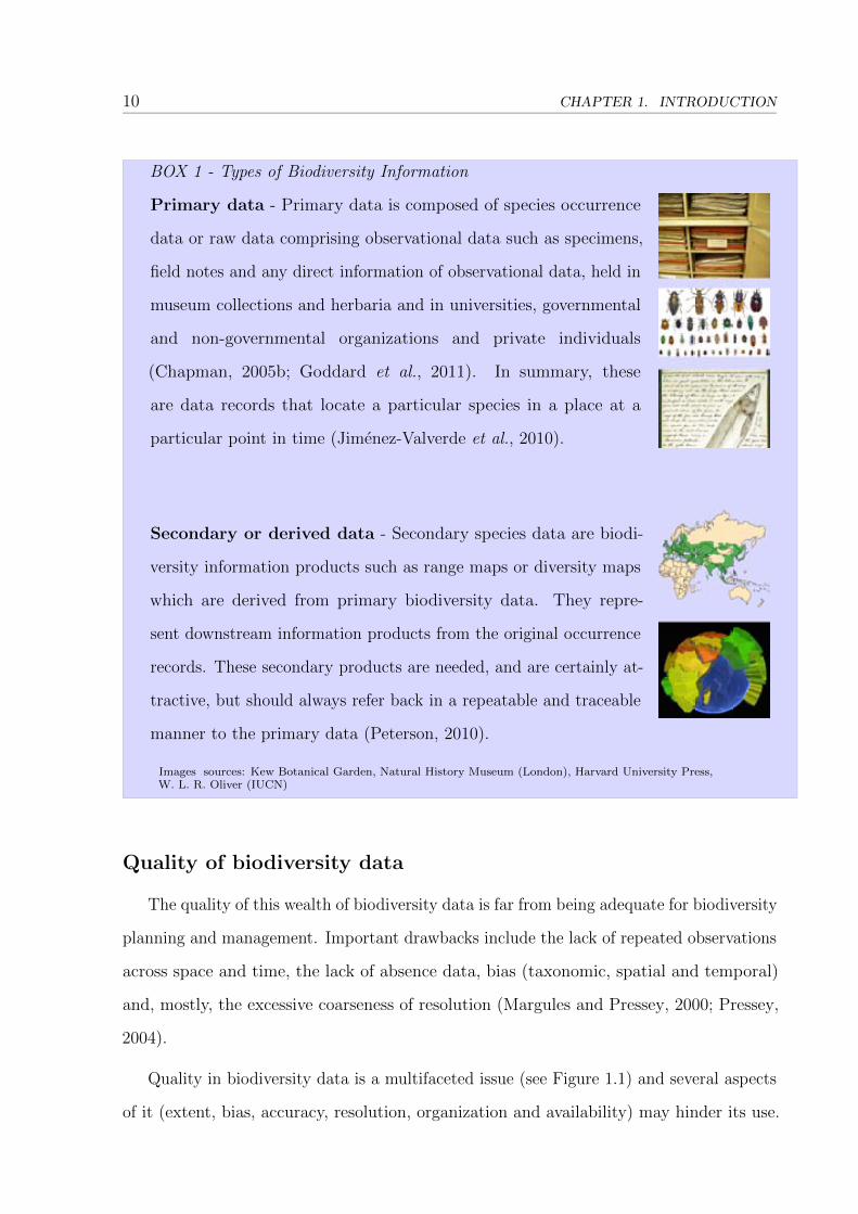
BOX 1 - Types of Biodiversity Information
Primary data - Primary data is composed of species occurrence
data or raw data comprising observational data such as specimens,
field notes and any direct information of observational data, held in
museum collections and herbaria and in universities, governmental
and non-governmental organizations and private individuals
(Chapman, 2005b; Goddard et al., 2011). In summary, these
are data records that locate a particular species in a place at a
particular point in time (Jimenez-Valverde et al., 2010).
Secondary or derived data - Secondary species data are biodi-
versity information products such as range maps or diversity maps
which are derived from primary biodiversity data. They repre-
sent downstream information products from the original occurrence
records. These secondary products are needed, and are certainly at-
tractive, but should always refer back in a repeatable and traceable
manner to the primary data (Peterson, 2010).
Images� sources: Kew Botanical Garden, Natural History Museum (London), Harvard University Press,W. L. R. Oliver (IUCN)
Quality of biodiversity data
The quality of this wealth of biodiversity data is far from being adequate for biodiversity
planning and management. Important drawbacks include the lack of repeated observations
across space and time, the lack of absence data, bias (taxonomic, spatial and temporal)
and, mostly, the excessive coarseness of resolution (Margules and Pressey, 2000; Pressey,
2004).
Quality in biodiversity data is a multifaceted issue (see Figure 1.1) and several aspects
of it (extent, bias, accuracy, resolution, organization and availability) may hinder its use.
1.2. BIODIVERSITY DATA 11
Figure 1.1: The dimensions of biodiversity data at the species level. Source: ownelaboration.
Being aware of these aspects and shortcomings and having them documented as metadata
is as important as solving them.
Extent The extent or comprehensiveness of the data clearly a�ects their usefulness in
biodiversity distribution studies. It is an obvious fact that in order to know or infer species
distributions in a particular area or region it is indispensable to have occurrence records
from that area or region. Biodiversity is spread all over the world; however, biodiversity
data is very patchy and concentrated in regions mainly of the developed world (Edwards
et al., 2000). For the vast majority of species, there is a shortage of data regarding their
actual distribution at varying scales (local, regional, global), i.e. the Wallacean shortfall.
Moreover, most data collections pertain to political or cultural geographical units hence
lacking in biological meaning (Whittaker et al., 2005). Not only the spatial extent is
important but also the temporal and taxonomic extent of the data. Temporal extent refers
to the time span for which there exist biodiversity observations. When modelling the

12 CHAPTER 1. INTRODUCTION
distribution of a given species it is important to have data that matches the temporal
span of the predictor variables used (Peterson et al., 2011). Taxonomic extent refers to
the number of taxons for which there is data; its lack known as Linnean shortfall.
Bias The quality of the data in relation to their extent is tightly bound to the
existence of bias. Bias refers to the probability with which a given site, species or time
will be sampled (Boakes et al., 2010). Biodiversity data tend to have taxonomic, spatial
and temporal bias (Boakes et al., 2010; Martin et al., 2012). This is due to the fact
that, for a given study area, most of it comes from ad hoc studies instead of planned
systematic surveys. Although data abound for parts of the world and for some speci�c
groups of species (e.g plants), in other large parts of the world and for the majority
of species, data describing distributions are very scarce (Newbold, 2010). Because the
environment is tightly coupled with geography. Spatial or geographical bias is implicitly
related to environmental bias. For species distribution modelling, the kind of bias that
a�ects predicted distributions is precisely the environmental bias rather than the spatial
bias.
Accuracy Accuracy measures the closeness of the observed value to the true value, e.g.
how close an observed x, y, z coordinate of a species observation is to the true coordinate
it occupies. This example refers to spatial accuracy, which a�ects georeferencing quality.
Even with groups such as plants and vertebrates for which a larger amount of digitised
data exists, a high-quality georeference for each specimen or citation is lacking (Anderson,
2012). Temporal accuracy is further facet of species occurrence data quality, but one which
is not usually limiting; most species distribution studies try to infer current or potential
distributions from occurrence data of a much �ner resolution than that of the expected
output map. Accuracy can also be applied at the taxonomic level and it re ects whether
species or taxons have been correctly identi�ed.
Resolution Research in biogeography, macroecology and conservation planning is often
based on the analysis of grid maps of species richness (Graham and Hijmans, 2006).
Knowing the spatial distribution of biodiversity at di�erent scales is an important issue in
1.2. BIODIVERSITY DATA 13
conserving it (Richardson and Whittaker, 2010). What is usually referred to as spatial
resolution is the size of grid cells (square being the most frequently used form). Occurrence
records can take di�erent types of georeferencing such as pairs of x,y coordinates and
toponyms. In any case, they are usually converted to grid form prior to modelling exercises,
except when they are already directly georeferenced as square grid cells (e.g. 1-by-1 km
Universal Transverse Mercator cells).
Despite the fact that the term resolution is normally associated with its spatial sense,
it needs also to be taken into account in its temporal and taxonomic sense. The former
relates to the size of the temporal interval to which a species occurrence is associated.
For example, a specimen in a natural history collection may have in its tag its year of
collection which would give us a resolution of 1 year. Poor temporal resolution is more
frequent with historical records, e.g. some old species observations can only be temporally
referenced to a century.
Taxonomic resolution is the classi�cation level at which a given individual is identi�ed,
from kingdom to levels below species (subspecies, varieties, etc.). The usual target unit
for modelling is that of species (Robertson et al., 2010). Lower resolution taxons such
as genus (e.g. Quercus sp., Bromus sp., . . . ) may be more di�cult to model due to the
diverse ecological requirements of the species they contain. Nevertheless, predicting their
distribution may be sensible in some studies (Marshall et al., 2006).
Organization Data organization is quite often not taken into account when considering
data quality, in spite of the fact that it ensures its consistency. Archiving in organized
repositories for the long-term storage of biodiversity data within a corporate infrastructure
with protocols for data entry is essential (Gioia, 2010). Ensuring a good design for the
organization of data, e.g. through the use of relational databases, is a crucial step to avoid
errors such as data duplication, orphaned keys and the like (Chapman, 2005a). Researchers
have at their disposal unprecedented computer power with which to use a plethora of
modelling techniques, old and new, which empowers them to perform sophisticated analysis.
Each software application which implements a modelling technique requires the data to
14 CHAPTER 1. INTRODUCTION
be fed in a speci�c custom-made format. Having correctly organized primary biodiversity
data has a big impact on the e�ciency with which it can be used in research, i.e. the time
needed for data preparation and curation for modelling purposes is all but negligible. The
more organized and documented through metadata the original primary data is, the easier
and better their conversion for the speci�c analysis at hand. Metadata allows for data
discovery, interpretation and appropriate use, and even automated use (Michener, 2006).
Availability Before being able to analyze and summarise biodiversity data into maps,
it is necessary to make all legacy and current data about when and where species oc-
cur available and easy to use (Guralnick and Hill, 2009). Even where formalized data
archiving is practised, this does not necessarily translate into easy access to data (Gioia,
2010). Despite remarkable progress in recent years, most biodiversity data in museum
holdings or literature remains unavailable in an adequate digital format. In the last three
decades, considerable e�ort has been put into the digitising of these data into publicly
available species distribution atlases. Such databases represent a wealth of data on species
distribution and an indispensable asset for science and conservation (Funk and Richardson,
2002; Graham et al., 2004; Suarez and Tsutsui, 2004; Franklin, 2009; Robertson et al.,
2010). Availability can also be considered a facet of quality; for data to be used it needs
to be readily available (e.g. through metadata-enabled discovery (Michener, 2006)). In
this respect, the computer revolution, database and GIS science and technology and the
Internet have become an indispensable tool in biodiversity research.
1.3 Mapping for biodiversity conservation
Conservation planning and management involve determining which areas need to be
managed for the persistence of biological diversity and natural values, a task which is
inherently spatial (Pressey et al., 2007). The range or geographic distribution of species
constitutes one of its fundamental dimensions (Anderson, 2012). Knowing the drivers that
cause changes in biodiversity and where they occur is also important for devising policies
for biodiversity conservation (Sala et al., 2000).

1.3. MAPPING FOR BIODIVERSITY CONSERVATION 15
Since we do not have detailed direct data on species distributions, reliable predictions
are necessary (Guisan et al., 2006b). We need tools to infer from incomplete data, often
scarce, where these values are located. In the case of species, intensive research and
development in recent years has produced a set of powerful inference tools for species
distribution modelling (see Figure 1.5). These are now available to exploit the wealth
of data increasingly held in easily accessible biodiversity databases for uses such as the
call for a reduction on biodiversity loss made by The Millenium Development Goals
and the Convention on Biological Diversity (United Nations Development Programme,
2009; Convention on Biological Diversity, 2010). Filling the biogeographical information
shortfalls and improving the accuracy of forecasts are challenges which lie ahead in the
�eld of conservation biogeography (Richardson and Whittaker, 2010; Ladle and Whittaker,
2011). In summary, we need maps of values, of threats and of sites to protect.
Maps of values. As it has already been stated, biodiversity refers to the variability of
life on Earth, at all its levels, from genes to ecosystems and biomes, which leads us to the
deduction that probably there should be conservation strategies in all of them. Arguably,
the most prominent discrete unit of biodiversity is that of species. Species provide us
with innumerable values and services: social, economical and spiritual. For these to be
preserved we �rst need to locate where they are distributed and what their ecological
requirements are; i.e we need maps. Given the sheer number of species on Earth, we have
to set priorities to allocate limited economic and human resources available.
Specially rich areas or hotspots (see Figure 1.2) need to be identi�ed and mapped in
order to optimally allocate these limited resources. Hotspots have exceptional concentra-
tions of endemic species which, at the same time, are under signi�cant habitat loss (Myers
et al., 2000). One of such areas is the Mediterranean basin. Current technologies and tools
can be used to perform �ne analysis of the distribution of species in hotspots susceptible
to be protected.
Maps of threats. Numerous studies exist that analyse the pressure or threats posed to
Earth's biodiversity (Sala et al., 2000; Petit et al., 2001; Gerard et al., 2010). Along with
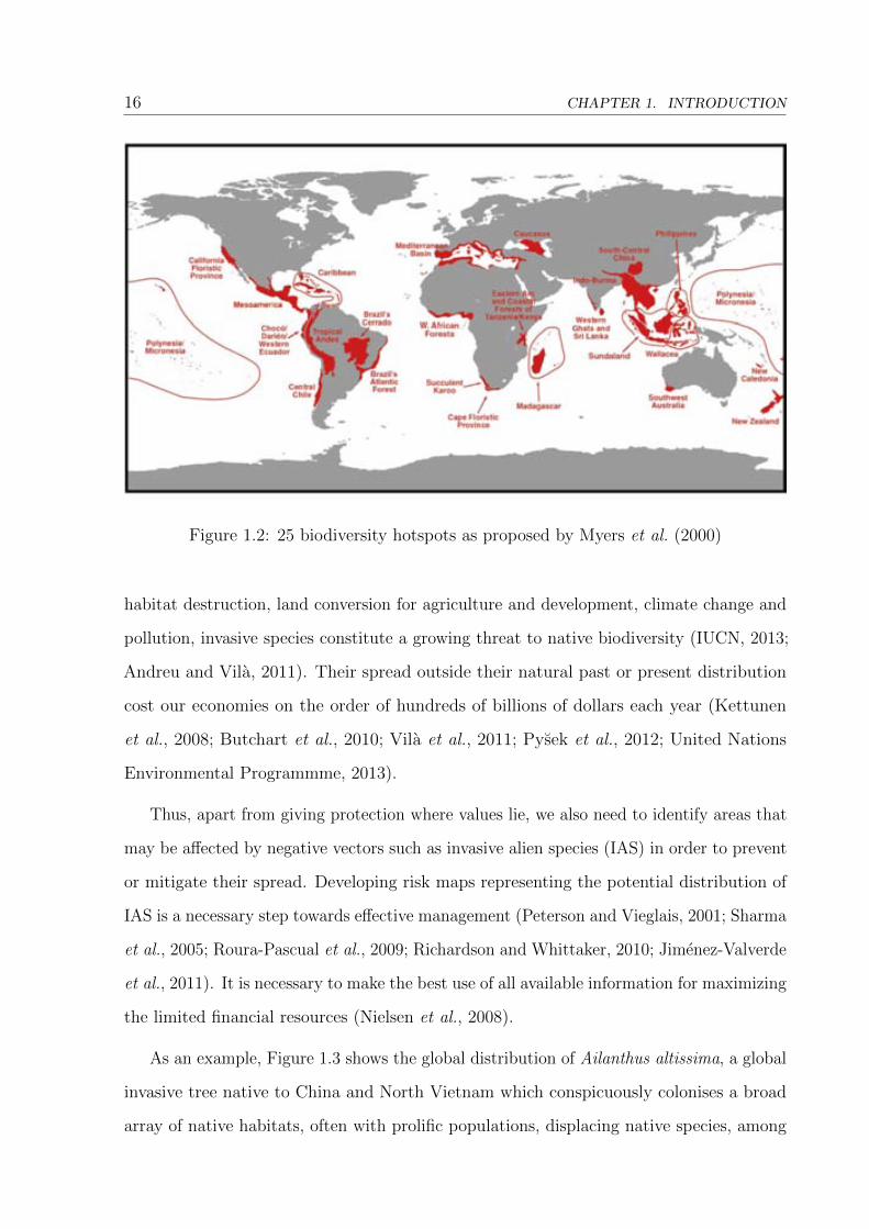
16 CHAPTER 1. INTRODUCTION
Figure 1.2: 25 biodiversity hotspots as proposed by Myers et al. (2000)
habitat destruction, land conversion for agriculture and development, climate change and
pollution, invasive species constitute a growing threat to native biodiversity (IUCN, 2013;
Andreu and Vil�a, 2011). Their spread outside their natural past or present distribution
cost our economies on the order of hundreds of billions of dollars each year (Kettunen
et al., 2008; Butchart et al., 2010; Vil�a et al., 2011; Py�sek et al., 2012; United Nations
Environmental Programmme, 2013).
Thus, apart from giving protection where values lie, we also need to identify areas that
may be a�ected by negative vectors such as invasive alien species (IAS) in order to prevent
or mitigate their spread. Developing risk maps representing the potential distribution of
IAS is a necessary step towards e�ective management (Peterson and Vieglais, 2001; Sharma
et al., 2005; Roura-Pascual et al., 2009; Richardson and Whittaker, 2010; Jim�enez-Valverde
et al., 2011). It is necessary to make the best use of all available information for maximizing
the limited �nancial resources (Nielsen et al., 2008).
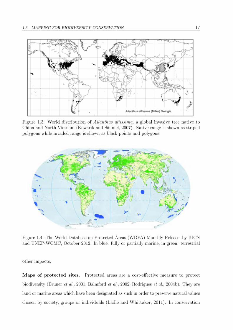
As an example, Figure 1.3 shows the global distribution of Ailanthus altissima, a global
invasive tree native to China and North Vietnam which conspicuously colonises a broad
array of native habitats, often with proli�c populations, displacing native species, among
1.3. MAPPING FOR BIODIVERSITY CONSERVATION 17
Figure 1.3: World distribution of Ailanthus altissima, a global invasive tree native toChina and North Vietnam (Kowarik and Saumel, 2007). Native range is shown as stripedpolygons while invaded range is shown as black points and polygons.
Figure 1.4: The World Database on Protected Areas (WDPA) Monthly Release, by IUCNand UNEP-WCMC, October 2012. In blue: fully or partially marine, in green: terrestrial
other impacts.
Maps of protected sites. Protected areas are a cost-effective measure to protect
biodiversity (Bruner et al., 2001; Balmford et al., 2002; Rodrigues et al., 2004b). They are
land or marine areas which have been designated as such in order to preserve natural values
chosen by society, groups or individuals (Ladle and Whittaker, 2011). In conservation

18 CHAPTER 1. INTRODUCTION
planning, boundaries of protected areas are a vital piece of information. Most protected
area boundaries have been delineated with incomplete knowledge of the distribution of
the biodiversity values they intended to protect (Rondinini et al., 2006), leaving gaps
of protection as a result. As more and more information becomes available and new
modelling tools are being developed, these gaps need to be assessed and solved (e.g.
through gap analysis (Scott et al., 1993)). To accomplish this, cartography on protected
areas' boundaries is needed. In order to assess the level of biodiversity protection we need
digital geodatabases on protected areas' boundaries (see Figure 1.4).
In summary, the combination of maps representing the values to preserve, the threats
to avoid and protected area boundaries can empower decision-makers when taking con-
servation actions. Species distribution modelling allows for the generation of distribution
maps out of occurrence data.
1.4 Species distribution modelling
Species distribution modelling (SDM) is a set of statistical tools which, by combining
observations of species occurrences and environmental data, allow us to hypothesise the
conditions under which species can survive, and thus to delimit the areas where we might
expect to �nd a species (Elith and Leathwick, 2009; Higgins et al., 2012). SDM is also
often cited under di�erent terms such as environmental niche modelling, ecological niche
modelling or habitat suitability modelling in the scienti�c literature.
SDM has experienced an explosive growth in recent years, enhanced by the increasing
general availability of occurrence data in digital databases, from sources such as natural
history collections and the scienti�c literature among others, and by new developments in
statistics and information technology (Graham et al., 2004; Phillips et al., 2006; Franklin,
2009; Elith and Leathwick, 2009; Peterson et al., 2011).
SDM can be aimed at answering two di�erent kinds of questions: a) why are species
distributed the way they are, and b) where are species distributed. In the �rst case, the
goal is to identify the environmental variables determining the distribution of the species

1.4. SPECIES DISTRIBUTION MODELLING 19
across geographical and environmental space. In the second case, the goal is to predict
where the species may be present. Each case serves di�erent purposes: in the �rst case,
understanding the ecological requirements and constraints of the species; and mapping
the species distribution, usually for conservation purposes (conservation planning, reserve
design, biodiversity assessment, etc.).
Justification for SDM. If we had direct occurrence data for every species at any
given scale and time frame, SDM would not be needed. Provided we also had extensive
environmental and biotic data, also at any given scale and time frame, we would be able
to calculate the environmental niche of any given species at any given moment in time.
However, such ideal conditions of data availability are far from being met even for any
given single species. Although in some cases data may seem abundant, they are still very
scarce for such a goal. Moreover, given the vast number of species and the limited human
and economical resources available, achieving this monumental task may never be in our
reach, at least in the foreseeable future. Given the global pressing conservation needs and
the need to understand how species respond to their environment, SDM are an invaluable
set of tools at our disposal.
SDM and data availability. In order to infer species distributions, we need data on
species presences and absences as well as data on the biotic and abiotic environments
which determine the ecology of species. With these, we can �t a function between the
response variable (presence/absence) and the set of independent variables or environmental
predictors (biotic and abiotic). With respect to the environmental predictors, while
there is a growing availability of extensive spatially-explicit data on abiotic predictors
(temperatures, precipitation, soil, etc.), extensive spatially-explicit data on biotic predictors
is rarely available. With respect to the response variable, the vast majority of data available
are only presences. Having data on species absences is the exception rather than the norm.
Moreover, when data on species absences is available, it is at least subject to discussion,
since true species absences from geographical space are very di�cult to con�rm (Anderson,
2003). Such situation about data requirements and availability has driven the development

20 CHAPTER 1. INTRODUCTION
of a plethora of modelling methods, speci�cally tailored to deal with di�erent scenarios of
data availability (see Figure 1.5). When only presence data is available several strategies
are possible (Figure 1.5): a) use only presences (BIOCLIM, HABITAT, DOMAIN, SVM),
b) create pseudoabsences by sampling the area where the species has not been cited
(GARP) and c) use only presences and compare them to the environmental background in
which they occur (MAXENT, ENFA).
Modelling without absence data
Methods that can infer species distributions from presence-only data are very much in
need since there are vast stores of such data held in natural museums and herbaria and
absence data is rarely available (Graham et al., 2004; Phillips et al., 2006). As we have
seen, several methods exist to model species distributions when there is no absence data.
Among these, the maximum entropy modelling approach (Maxent) stands out among
the best performers for this kind of data even when data are scarce (Elith et al., 2006;
Hernandez et al., 2006; Phillips and Dud��k, 2008; Wisz et al., 2008; Elith and Graham,
2009; Thorn et al., 2009; Costa et al., 2010) and bias is present (Rebelo and Jones, 2010).
Although Maxent is not a strict presence-only method like BIOCLIM or DOMAIN, it has
better discriminatory power (Peterson et al., 2011). Maxent uses presence-only data in
combination with data on environmental variation across the study area, background data
in Maxent terms.
Maximum entropy modelling Maxent is a general-purpose method for making pre-
dictions or inferences from incomplete information. It originates in the �eld of statistical
machine learning and is widely used in other knowledge �elds as diverse as astronomy,
signal processing or natural language processing (Jaynes, 1957; Phillips et al., 2004, 2006).
Recently, this modelling technique has been widely used by the species distribution mod-
elling community thanks to the fact that it has been adapted, made easily available
through a speci�cally-developed software package (with a user-friendly interface), tested
and speci�cally explained for ecologists (Phillips et al., 2004, 2006; Elith et al., 2011).
There are abundant examples of its application to many kinds of distributional studies:

1.4. SPECIES DISTRIBUTION MODELLING 21
species richness (Newbold et al., 2009), invasive species (O'Donnell et al., 2012), climate
change e�ects on species distributions (Franklin et al., 2012), endemism areas (Herzog
et al., 2012), protection quality (N�obrega and De Marco Jr, 2011) and rare species (Marino
et al., 2011) among others.
Maxent (Phillips et al., 2004, 2006; Elith et al., 2011) uses data on the environmental
background on which the species exists and tries to estimate a probability distribution
which is the most uniform or spread out and, at the same time, which satis�es the
constraints imposed by the available occurrence records and the environments in which
they occur but no more (Phillips et al., 2006). In other words, it estimates the target
distribution of the species with maximum entropy, subject to the constraint that the
expected value of each feature under this estimated distribution matches its empirical
average. This distribution agrees with only what is actually known and avoids assumptions
not supported by the data. According to its authors (Phillips et al., 2006), its main
advantages are: a) it requires only presence data and environmental information for the
study area, b) it works with both continuous and categorical data and their interactions,
c) it is deterministic and amenable to mathematical analysis, d) over-�tting is avoidable,
e) bias can be treated, f) output is continuous, which allows to set di�erent thresholds
to produce binary maps and, g) it works well with scarce data. Its main disadvantages
are: a) it is not as mature a method as other classical statistical approaches such as GLM
(Nelder and Wedderburn, 1972) or GAM (Hastie and Tibshirani, 1986), b) regularization
needs to be studied and applied to overcome over-�tting, and c) it needs speci�c software.
The software package o�ers the possibility to work on Auto features mode, which means
that Maxent decides which kind of functions to �t depending on the nature of the data it
is fed. This is a widely used operating option since Maxent has already been calibrated to
work with di�erent species pertaining to di�erent taxonomic groups, with di�erent number
of occurrence records and di�erent species prevalence (Phillips and Dud��k, 2008). The user
has the freedom to choose among di�erent �tting possibilities (linear, quadratic, product,
threshold and hinge). The hinge option approximates it to a GAM (Elith et al., 2011).
The output of Maxent are raw probabilities which sum to one across the whole studied

22 CHAPTER 1. INTRODUCTION
area and is, hence, scale dependent (Phillips and Dud��k, 2008). Since the raw format in
Maxent can be di�cult to interpret, recent versions of Maxent include a logistic output
which estimates the probability of presence or suitability of the site for the species (Phillips
and Dud��k, 2008). However, since absence data is not used, results should be interpreted
as potential relative suitabilities of each site of the study area in relation to the general
background available (Phillips et al., 2006). In order to estimate a true probability of
presence, information on absences should also be available and fed to the model (Peterson
et al., 2011).

1.4. SPECIES DISTRIBUTION MODELLING 23
Fig
ure
1.5:
Mai
nsp
ecie
sdis
trib
uti
onm
odel
ling
met
hods
by
typ
esof
dat
a.Sou
rce:
Ow
nel
abor
atio
n,
par
tial
lybas
edon
Fra
nklin
(200
9)an
dP
eter
son
etal
.(2
011)
.
24 CHAPTER 1. INTRODUCTION
Model calibration and validation
When calibrating a model it is necessary to have a clear conceptualization of the
parameters involved and the extent of that study area. In this respect, Sober�on and
Nakamura (2009) proposed the BAM diagram, a heuristic scheme useful for analyzing the
interplay between movements, abiotic and biotic environments (see Box 2).
In model calibration, parameters are adjusted so that model output validation achieves
a de�ned degree of performance, i.e. agrees with observed data. Datasets for calibration
and validation should be independent of each other. In an ideal situation, a separate
independent set of occurrence data would be held out of calibration data and would be
used to evaluate the performance of the generated model. The main goal of calibration is
to develop a model that �ts well to data but which, at the same time, does not over-�t
(Peterson et al., 2011), that is, it works well with other sets of data.
When calibrating a model, the choice of environmental predictors is an important
decision. They should be chosen based on biological reasons (Elith and Leathwick, 2009),
i.e. variables known or suspected to have an in uence on limiting the distribution of the
species being modelled at the given scale and time frame. Very often, this information
is not known before running the model itself. Actually, the modelling process itself is
often used to determine which variables a�ect species distribution. Usually, an iterative
sequence of model runs helps in deciding the best �nal set of predictors. Another issue
to take into account is the autocorrelation among predictors since it can hinder model
interpretation (Dormann et al., 2008). A possible solution is using principal component
analysis to transform the variables into a set of orthogonal uncorrelated variables. However,
when the purpose of the study is predictive only, as in this thesis, autocorrelation can
be left untreated as it does not a�ect Maxent predictive performance (Kuemmerle et al.,
2010).
1.4. SPECIES DISTRIBUTION MODELLING 25
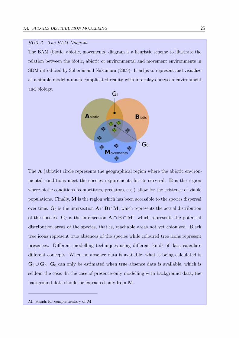
BOX 2 - The BAM Diagram
The BAM (biotic, abiotic, movements) diagram is a heuristic scheme to illustrate the
relation between the biotic, abiotic or environmental and movement environments in
SDM introduced by Soberon and Nakamura (2009). It helps to represent and visualize
as a simple model a much complicated reality with interplays between environment
and biology.
The A (abiotic) circle represents the geographical region where the abiotic environ-
mental conditions meet the species requirements for its survival. B is the region
where biotic conditions (competitors, predators, etc.) allow for the existence of viable
populations. Finally, M is the region which has been accessible to the species dispersal
over time. G0 is the intersection A∩B∩M, which represents the actual distribution
of the species. GI is the intersection A ∩B ∩Mc, which represents the potential
distribution areas of the species, that is, reachable areas not yet colonized. Black
tree icons represent true absences of the species while coloured tree icons represent
presences. Different modelling techniques using different kinds of data calculate
different concepts. When no absence data is available, what is being calculated is
G0 ∪GI . G0 can only be estimated when true absence data is available, which is
seldom the case. In the case of presence-only modelling with background data, the
background data should be extracted only from M.
Mc stands for complementary of M
26 CHAPTER 1. INTRODUCTION
With respect to occurrence data, it is often the case that no independent dataset
on which to evaluate performance is available. Under these circumstances, an accepted
approach is to randomly choose a given percentage of occurrences, not to be used during
the calibration process, and keep them apart as a test dataset. A better approximation
are cross-validation techniques, usually k -fold cross-validation (Fielding and Bell, 1997).
In k -fold cross-validation, the available dataset is divided into k groups. Then, the model
is built with k-1 groups and the kth group is used for validation. This procedure is then
repeated k times until all groups have been used for validation. A particular case of
cross-validation is the leave-one-out technique, in which, as its name indicates, groups are
composed of one single occurrence (k equals the number of occurrences). Leave-one-out
techniques are a useful option when data are very scarce (Pearson et al., 2007). Still
another option is bootstrap sampling, i.e. sampling with replacement. Cross-validation
techniques ensure that any given point is used both in calibration and in testing. Also, k
estimates of accuracy are obtained, which can then be averaged to have a �nal performance
estimate with standard deviation. Finally, a measure of �t of the model to the data is
obtained.
Performance measures The accuracy of species distribution models needs to be quan-
ti�ed in order to evaluate predictive ability. Predictive ability or performance refers to how
close the predicted distribution is to the observed data and hence to the actual distribution.
However, questions such as how credible the model is in ecological terms should also
be addressed, specially when the modelling aim is to explain the species distribution
(Franklin, 2009). Errors are inherent to modelling since models are approximations to
the real world which leave unexplained variance. Errors can arise from factors such as
model misspeci�cation (e.g. choosing an inadequate set of predictors), data errors (e.g.
introducing spatial error when georeferencing or misidentifying a species) and choice of an
inadequate modelling technique, among others.
Model outputs are in the form of continuous probability maps. If, as in most cases, the
desired outcome are binary maps (presence/absence or suitable/unsuitable areas), they
need to be converted by setting a cut-o� threshold. All sites, i.e. pixels or grid cells, with
1.4. SPECIES DISTRIBUTION MODELLING 27
a probability value below the selected threshold are assigned to 0 and the rest to 1. With
a binary map the performance of a model, how it classi�es each occurrence point, can be
evaluated. There are two types of model performance measures: a) threshold-independent,
which evaluate performance across all thresholds and, b) threshold-dependent, whose
performance evaluation is bound to a speci�c threshold.
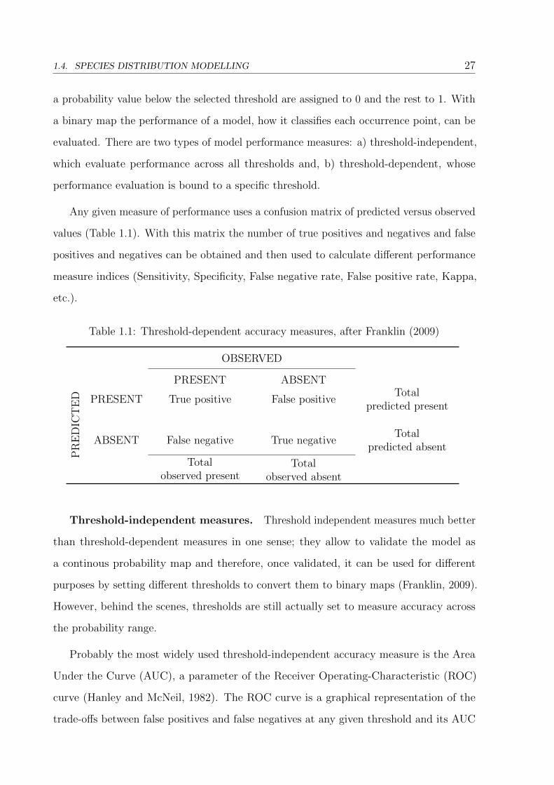
Any given measure of performance uses a confusion matrix of predicted versus observed
values (Table 1.1). With this matrix the number of true positives and negatives and false
positives and negatives can be obtained and then used to calculate di�erent performance
measure indices (Sensitivity, Speci�city, False negative rate, False positive rate, Kappa,
etc.).
Table 1.1: Threshold-dependent accuracy measures, after Franklin (2009)
OBSERVED
PRESENT ABSENT
PR
ED
ICT
ED PRESENT True positive False positive
Totalpredicted present
ABSENT False negative True negativeTotal
predicted absent
Totalobserved present
Totalobserved absent
Threshold-independent measures. Threshold independent measures much better
than threshold-dependent measures in one sense; they allow to validate the model as
a continous probability map and therefore, once validated, it can be used for di�erent
purposes by setting di�erent thresholds to convert them to binary maps (Franklin, 2009).
However, behind the scenes, thresholds are still actually set to measure accuracy across
the probability range.
Probably the most widely used threshold-independent accuracy measure is the Area
Under the Curve (AUC), a parameter of the Receiver Operating-Characteristic (ROC)
curve (Hanley and McNeil, 1982). The ROC curve is a graphical representation of the
trade-o�s between false positives and false negatives at any given threshold and its AUC
28 CHAPTER 1. INTRODUCTION
relates to the probability of ranking higher a species presence than a species absence. In
this kind of plots, an AUC of 0.5 means that the classi�er is not better than random and
above 0.5 that the classi�er is better than random. When evaluating presence-only models,
this measure can be interpreted as an indication of the discrimination between presence of
the species and background rather than presence and absence (Phillips et al., 2009). Liu
et al. (2009) lists other threshold-independent measures of accuracy which can be used in
SDM, among them the Maximum Overall Accuracy, the Maximum kappa, the Gini index
and the point biserial correlation coe�cient.
Threshold-dependent measures. In contrast with threshold-independent mea-
sures of performance, these measures refer only to a given threshold value. If di�erent
thresholds need to be used for the purpose at hand, then each generated binary map needs
to be evaluated separately. Prior to measuring accuracy a threshold must be set to convert
models to binary maps. There are many di�erent options for threshold setting and they
have been discussed by many authors (Liu et al., 2005; Jim�enez-Valverde and Lobo, 2007;
Freeman and Moisen, 2008; Nenz�en and Ara�ujo, 2011; Jim�enez-Valverde, 2012; Bean et al.,
2012). Many of the threshold options rely on having both presence and absence data,
which is not available in presence-only modelling. Without absence data these thresholds
cannot be calculated. For presence-only data, several thresholding options exist, among
them: �xed threshold like 0.5 (Li et al., 1997; Manel et al., 1999; Bailey et al., 2002),
Minimum Predicted Area (MPA) (Engler et al., 2004) and Minimum Training Presence
(MTP) (Pearson et al., 2007).
The �xed threshold option is quite an arbitrary one and could be left to cases where
a very conservative approach is needed, e.g. if 0.5 is chosen anything any better than
random will be predicted as present/suitable, or also, when a prede�ned overall predicted
area is needed. The other two thresholds are much more meaningful. MPA minimizes
omission errors and the area predicted to be suitable. Models with lower MPAs are
more parsimonius and, therefore, could be considered better (Franklin, 2009). The MTP
threshold is equivalent to the lowest estimated value at the site of any occurrence point.
This option sets the cut-o� at a point where, by de�nition, all observed occurrence records

1.4. SPECIES DISTRIBUTION MODELLING 29
will fall inside the predicted area, thus ensuring a zero omission rate. MTP is a very
appropriate option when the purpose is to de�ne suitable areas for conservation with a set
of occurrence data which is known to be free of georeferencing and identi�cation errors.
Also, MTP makes sense ecologically since it includes all sites that are at least as suitable
as those where the species has been recorded as present (Pearson et al., 2007).
Model outputs: distribution or range maps
Species distribution or range maps re ect either the species presence or its terrain-
suitability across geographical space; which is very useful information in conservation
planning and management (Robertson et al., 2010). Species richness across space is very
heterogenous (Gaston, 2000) due to the widely di�erent types of species distributions:
scattered, clustered, etc. Species distribution can be de�ned as the set of all grid elements
in a speci�c sampling period of time where the probability of �nding the species exceeds
some given threshold (Peterson et al., 2011).
Knowledge of species distributions or ranges is necessary to elaborate speci�c action
plans for their conservation and ensure their inclusion in protected areas, two important
conservation actions to ensure species survival (Cuttelod et al., 2008). Several methods
exist to generate species range maps: point occurrence data, expert-drawn maps, species
distribution models and hybrid approaches (Graham and Hijmans, 2006). Before the
availability of modern modelling techniques and extensive digital readily-available envi-
ronmental data, range maps needed to be drawn by expesrts or directly derived from
observations in grid format. Currently, SDM allow us to infer probability maps of species
presence which, in conjunction with threshold setting, can be converted into binary maps,
i.e. range maps.
The species' range area of these maps depends on the scale at which they are generated.
In general, since species can not be mapped down to the actual size of their individuals,
they must be generalized to some spatial resolution value. Modelled species range maps
can then be used to assess species conservation and protection and to generate maps of
biodiversity richness and hotspots by overlaying individual species maps, which can then

30 CHAPTER 1. INTRODUCTION
be used in biodiversity conservation planning. Also, when applied to alien invasive species,
these maps can be used to guide conservation actions speci�cally tailored to avoid species
invasions and the resulting impoverishment in native biodiversity (e.g. Thuiller et al.
(2005); Wilson et al. (2007); V�aclav��k and Meentemeyer (2012)).
Use of species range maps in conservation
Distribution or range maps derived from SDM have important direct applications
in conservation: biodiversity discovery (populations, species limits, unknown species),
conservation planning, species reintroductions, vulnerability to invasion, planning protected
areas, etc. (Peterson et al., 2011). Species geographic ranges, and their change over time
represent fundamental ecological and evolutionary characteristics of species which have
direct use in assessing and predicting extinction risk (Gaston, 2003), a fundamental concept
in conservation biology.
Species ranges and risk of extinction Range size is one of the main measures in
evaluating the risk of exinction of a given species. In particular, two measures of size are
used for such purpose, the Extent Of Occurrence (EOO) and the Area Of Occupancy
(AOO). IUCN (2001) de�nes EOO as the area contained within the shortest continuous
imaginary boundary which can be drawn to encompass all the known, inferred or projected
sites of present occurrence of a taxon, i.e. the area that lies within the outermost
geographic limits of the occurrence of a species. It is normally measured by the method of
the minimum convex polygon or convex hull of all occurrence data. AOO is de�ned as the
area within its EOO which is occupied by a taxon, excluding cases of vagrancy (IUCN,
2001). The size of the AOO is dependent on the scale, the grain size or resolution, used to
map the species. IUCN suggests to use a grid size of 2x2 km to measure it. EOO and
AOO measures are used in criteria B1 and B2 of IUCN red listing guidelines (IUCN, 2001;
IUCN Standards and Petitions Subcomittee, 2011).
Analyzing species protection Protected areas are a crucial tool in reducing the
risk of species extinction, hence in conserving the world's biodiversity (Rodrigues et al.,
2003; Chape et al., 2005; Barr et al., 2011; Butchart et al., 2012) and thus, in reducing
1.4. SPECIES DISTRIBUTION MODELLING 31
the risk of species extinction. The combination of spatially-explicit models of species
of conservation interest with existing reserve networks can be a very powerful tool in
conservation management and planning.
These types of analysis are paramount to answering a question of importance to
the conservation of biological diversity: how e�ective are protected areas at conserving
biodiversity ? (Margules and Pressey, 2000; Brooks et al., 2004; Chape et al., 2005;
Langhammer et al., 2007; Suthterland et al., 2009). This can be answered by gap analysis
(Scott et al., 1993; Rodrigues et al., 2003; Brooks et al., 2004; Dudley and Parish, 2006;
D'Amen et al., 2013).
Systematic use of gap analysis is an important tool in identifying conservation gaps,
provide conservation information for conservation managers, guide speci�c resource man-
agement activities and mitigation actions to counter the e�ect of climate change (U.S.
Geological Survey, 2013; United Nations Environment Programme, 2013). Gap analysis
is interpreted as a strategy for achieving comprehensive, representative and e�ectively
managed networks of protected areas. In gap analysis, explicit biodiversity representation
targets are spatially set and then compared to the existing network of protected areas in
order to analyze to which degree they are met. Then, priorities for expanding the protected
area network, based on the principles of irreplaceability and vulnerability, are identi�ed to
achieve the targets for all features (Langhammer et al., 2007). This information can then
be combined with spatial layers of land ownership, stewardship and management status in
order to correctly direct conservation action (Scott et al., 1993; Jennings, 2000).
Preventing IAS spread Not only identifying the intersection between conservation
targets and reserve networks is important but also the intersection of these with threats. In
this respect and as we have previously seen, IAS are one of such threats. The ever-increasing
number of alien species and the costs associated with them justi�es the development of
preventive risk management plans or strategies (Sandlund et al., 1999; Pimentel et al.,
2005; Andreu and Vil�a, 2010). These can be enhanced by the generation of risk maps of
potential IAS spread, particularly so in protected areas, if they provide one of the main

32 CHAPTER 1. INTRODUCTION
tools in biodiversity protection and safeguard native species from extinction. These risk
maps are a necessary step towards e�ective management (Jim�enez-Valverde et al., 2011;
Richardson and Whittaker, 2010) and resources should be focused where they will achieve
the greatest bene�t (van Wilgen et al., 2011).
An important point to be taken into consideration when modelling IAS is that they may
not have reached equilibrium in their new invaded environment, an important assumption
in species distribution modelling (V�aclav��k and Meentemeyer, 2009). IAS are normally not
in equilibrium but in the process of expansion in a new environment and thus, extrapolation
is needed (Kearney, 2006; V�aclav��k and Meentemeyer, 2012). However, in certain areas
where IAS have been established for an extended period of time, this equilibrium can be
assumed (Williamson et al., 2009; Gass�o et al., 2010) and SDM used safely in this respect.
1.5 Biodiversity Conservation Information Systems
Knowledge about biodiversity is paramount to its conservation; even more so if we
take into account the pressing needs set by the ever increasing risk of biodiversity loss due
to human action. In order to gain this knowledge, data at all levels is needed, both from
the research and management domains: from genes to biomes and from local conservation
actions to global ones. Two types of very speci�c and important data for conservation
management and planning are species occurrence data and protected area boundaries.
Primary data on biodiversity has been captured over the decades in an unstructured,
analog form: museum collections, scienti�c and technical literature, cartographical sheets,
etc. Data such as taxon lists, species geographical atlases or protected area boundaries
were compiled with a local, regional or national focus and each item represented at a single
scale or resolution. There are vast quantities of them which need to be collected, organised
and made accessible in order to be put to use in conservation research, management
and planning. Biodiversity and protected areas information is needed in the research
domain, and governmental organisations are required and recommended by competent
bodies to make all this information public (European Environment Agency, 2007; Moritz
1.5. BIODIVERSITY CONSERVATION INFORMATION SYSTEMS 33
et al., 2011). Currently many di�erent institutions around the world are in the process of
digitising this information. Safeguarding them through databasing with georeferences and
date stamps is critical (Boakes et al., 2010).
In the last decades, there has been a huge increase in the availability of digitised
information on biodiversity and protected areas in the form of GIS layers and geodatabases
(Newbold, 2010). However, the simple translation from analogical to digital format is
not su�cient. The relevant information they contain needs to be isolated and coded in
some sort of structured format (database, xml, etc.) to make them readable by software
agents. Georeferenced databases on the distribution of both protected areas and species is
critically important, yet neither their structure nor their content is su�cient for the task
of analyzing distributional patterns and coverage degree (Brooks et al., 2004).
Since biodiversity data are complex, sophisticated information architectures are needed
to handle them. With the advent of the digital revolution, we now have the tools
to standardise, homogenise and aggregate this information. Current information and
communication technologies o�er an unprecedented opportunity to greatly enhance the
handling, analysis and public dissemination of environmental information (Sober�on and
Peterson, 2004). Information systems are technological solutions aimed at solving the
capture, storage, analysis and retrieval of data on a given knowledge �eld. Once in an
information system, all sorts of outputs can be obtained from these data, e.g. simple
queries, automated lists and reports, web mapping tools or species distribution maps
derived from modelling tools. The combination of these needs and the current technological
revolution has led to the emergence of the new �eld of biodiversity informatics, which
deals with the application of information technologies to the management, algorithmic
exploration, analysis and interpretation of primary data regarding life, particularly at the
species level of organisation (Sober�on and Peterson, 2004).
Handling biodiversity data for research or management purposes, even if in digital
format, is a very time consuming task. Data needs to be prepared and organised for every
task at hand. In order to make the most e�cient use of researchers' and managers' time,
access and analysis of these data needs to be made as agile as possible. This requires data

34 CHAPTER 1. INTRODUCTION
in an integrated, coherent repository which obeys common standards such as common
reference systems, controlled vocabularies, coding schemes and the like. In order to make
the best use of both geographical and biological information, it must be captured in a
standardised format to allow the union and intersection of both types of information
(Reusser and Lee, 2011).
Not only homogenising and structuring the data is important but also the tools
needed to exploit this information. Conservation Information Systems must deal with
heterogeneous geographical and ecological data (alphanumerical attributes, vector and
raster maps, documents, images, etc.) and information systems should provide the means
to deal with all this kind of data in an integrated manner. It is necessary to hand
researchers and managers comprehensive tools which allow to reach all these data from
the same system, instead of via di�erent software tools (da S. Torres et al., 2006; Reusser
and Lee, 2011). The pipeline between suppliers and users needs to be cleared. We need
systems whereby data of di�erent kinds, from many sources, can be combined (Scholes
et al., 2008).
A desired scenario of would be that of a centralized gateway to data repositories
of worldwide information on species occurrences which can be queried for standardised
well-structured metadata-enhanced datasets on any given species for any given region
and time period. Modelling tools, software packages, would understand and accept some
sort of agreed format on species occurrence data as input. This would free modellers
from the tedious and time-consuming task of data compilation and preparation, freeing
them to focus only with the problem at hand, saving countless hours of data management.
This scenario has not been achieved yet. However, several initiatives are clearly going in
that direction, the most prominent one being that of the Global Biodiversity Information
Infrastructure or GBIF (GBIF, 2013a).
From the point of view of information access, uni�ed repositories of data can be
achieved by di�erent means. A �rst obvious one is to design and develop a unique, central
geodatabase containing all data coming from many di�erent sources. This requires technical
sta� which has previously homogenised and integrated the information (an example of it
1.5. BIODIVERSITY CONSERVATION INFORMATION SYSTEMS 35
would be the World Database on Protected Areas, see below). A second option would
be that of a federated or virtual database where data can be accessed through a single
data portal which retrieves information from di�erent separate databases through a web
services gateway (an example of it would be GBIF, see below). A distributed database
is comprised of loosely coupled sites, connected over a computer network and hosted in
separate computing facilities which may not even be in the same physical location. With
this option, there needs to be a compromise on basic standards between the di�erent
institutions hosting the distributed databases so that the system can function properly.
The hosting institutions may hold their data in very di�erent systems but must agree to a
given standard and web service of data interchange. In summary, the di�erent systems
must be interoperable, i.e. each system must be accessible by other systems without
signi�cant human and technical interaction (Mas�o, 2012). In this scenario, each institution
is responsible for data stewardship and curation. In order to avoid dealing with the
expensive task of collecting and organising information, a third option, far-fetched at the
moment, would be needed. This would need arti�cially intelligent systems which can
interpret unstructured and non-standardised information on their own and provide us with
digested information. Meanwhile, the development of user-friendly, robust information
systems is a must.
The need for readily available biodiversity information has been acknowledged at
all levels, from local to regional, national and global institutions (governmental, non-
governmental and international organisations) and there are innumerable initiatives (see
Box 3 for some of the most relevant) at all these scales to collate such information in
publicly available databases. Some leading international initiatives have become the leaders
in terms of setting standards and in collecting and providing species and protected areas
data: the Global Biodiversity Information Facility (GBIF) and the World Database on
Protected Areas (WDPA), respectively.
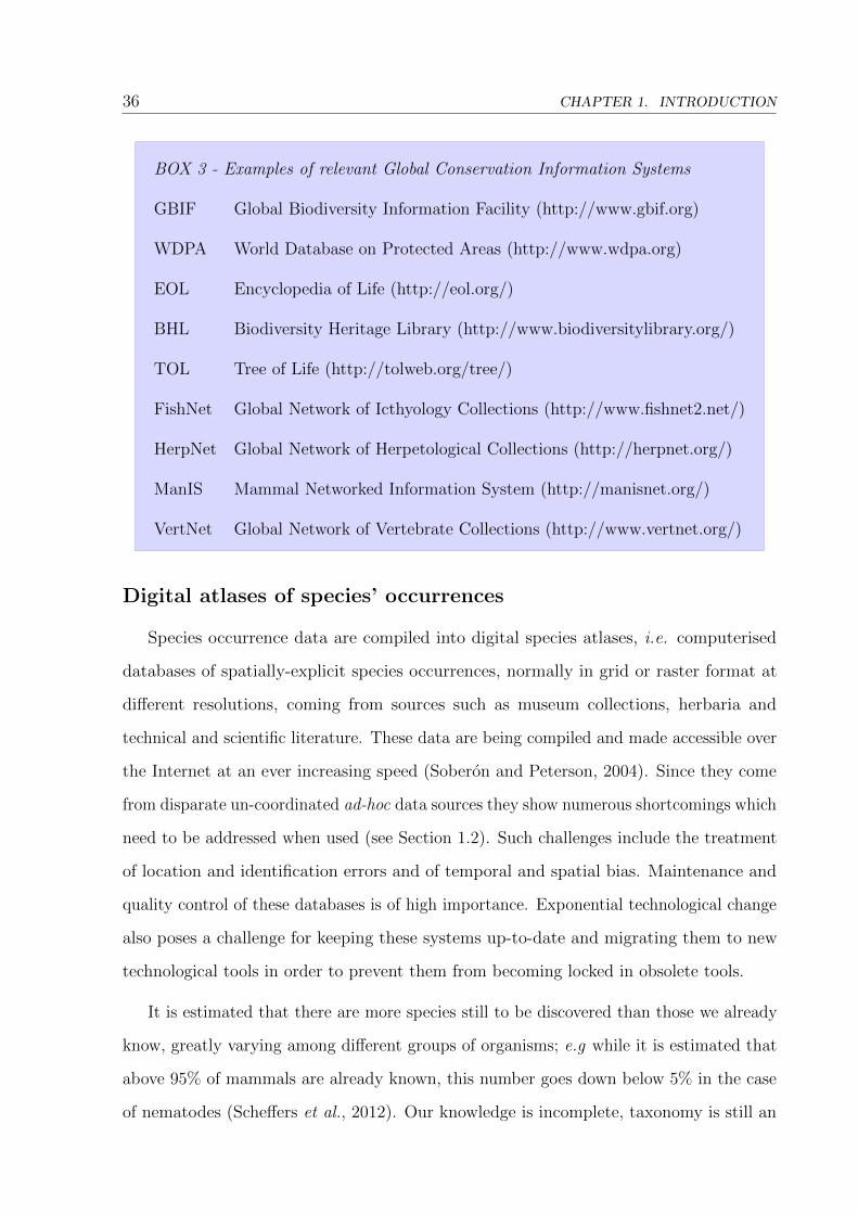
36 CHAPTER 1. INTRODUCTION
BOX 3 - Examples of relevant Global Conservation Information Systems
GBIF Global Biodiversity Information Facility (http://www.gbif.org)
WDPA World Database on Protected Areas (http://www.wdpa.org)
EOL Encyclopedia of Life (http://eol.org/)
BHL Biodiversity Heritage Library (http://www.biodiversitylibrary.org/)
TOL Tree of Life (http://tolweb.org/tree/)
FishNet Global Network of Icthyology Collections (http://www.�shnet2.net/)
HerpNet Global Network of Herpetological Collections (http://herpnet.org/)
ManIS Mammal Networked Information System (http://manisnet.org/)
VertNet Global Network of Vertebrate Collections (http://www.vertnet.org/)
Digital atlases of species’ occurrences
Species occurrence data are compiled into digital species atlases, i.e. computerised
databases of spatially-explicit species occurrences, normally in grid or raster format at
di�erent resolutions, coming from sources such as museum collections, herbaria and
technical and scienti�c literature. These data are being compiled and made accessible over
the Internet at an ever increasing speed (Sober�on and Peterson, 2004). Since they come
from disparate un-coordinated ad-hoc data sources they show numerous shortcomings which
need to be addressed when used (see Section 1.2). Such challenges include the treatment
of location and identi�cation errors and of temporal and spatial bias. Maintenance and
quality control of these databases is of high importance. Exponential technological change
also poses a challenge for keeping these systems up-to-date and migrating them to new
technological tools in order to prevent them from becoming locked in obsolete tools.
It is estimated that there are more species still to be discovered than those we already
know, greatly varying among di�erent groups of organisms; e.g while it is estimated that
above 95% of mammals are already known, this number goes down below 5% in the case
of nematodes (Sche�ers et al., 2012). Our knowledge is incomplete, taxonomy is still an
1.5. BIODIVERSITY CONSERVATION INFORMATION SYSTEMS 37
evolving endeavour and phylogenetic trees are being re�ned continuously. Without an
inventory list of the world's species, and still in the process of checking if every species
is correctly classi�ed, developing a spatially-enabled biodiversity database is a daunting
challenge, yet unavoidable given the pressing conservation needs. Whatever knowledge we
have needs to be put to use in conservation.
Among digital species atlases, GBIF stands out as the largest single gateway to species
occurrence data which is global in scope (Yesson et al., 2007).
Protected areas’ databases
The part of the present dissertation which deals with information systems concentrates
on protected areas databases. The importance of protected areas in preserving biodiversity
and serving as a surrogate indicator of biodiversity makes the organisation of information
on protected area boundaries in digital geodatabases a very important task for conservation
evaluation. Besides being usable by itself, protected area boundaries can be combined
with models of distributions of species of conservation interest to perform gap analysis
and determine where conservation e�orts should be placed (Scott et al., 1993; Rodrigues
et al., 2004b; Langhammer et al., 2007; United Nations Environmental Programme, 2008;
Jantke et al., 2011) and with models of distributions of IAS to determine the risk of
invasion (Richardson and Whittaker, 2010). Advances in data availability and in the
science of conservation planning enable us to act strategically in the face of increasing
human pressure (Rodrigues et al., 2004b). As is the case with biodiversity data, protected
area boundaries need to be homogenised and integrated into geodatabases. This will ease
its use in gap analysis and biodiversity protection assessments. In this respect, the World
Database on Protected Areas (IUCN-UNEP, 2010) is the most comprehensive dataset on
the world's terrestrial and marine protected areas. Other databases are only national or
supra-national in scope, such as the Collaborative Australian Protected Area Database
(Australian Department of the Environment, Water, Heritage and the Arts, 2008), the
Protected Areas Database of the United States(GreenInfo Network, 2008) or the European
Common Database on Designated Areas (European Environment Agency, 2009c), to cite

38 CHAPTER 1. INTRODUCTION
the largest three.
An important but often neglected aspect on the information of protected areas bound-
aries is time. Protected areas are not static legal entities over time but undergo changes in
their regulations which follow the legal and socioeconomic contexts at any given moment.
These changes may not only a�ect the existing set of regulations but also their boundaries;
i.e. they get extended, reduced, reclassi�ed, amalgamated with neighbouring sites, re-
named, etc. (Fish et al., 2005). Having structured historical information on protected-area
boundaries for all protection categories in a given territorial extent allows to monitor
protected-area coverage over time and, thus, biodiversity protection. Also, it is possible
to explore the social, economical and political factors driving changes in protected-area
coverage and thus, hopefully, discover some hidden socioeconomic processes or drivers
which govern how society decides whether to value and protect biodiversity.
1.6 Dissertation structure
This dissertation is structured as follows:
� Chapter 2 deals with the distribution modelling of rare species of conservation
interest in order to obtain maps for assessing the degree of protection and extinction
risk. Several narrowly distributed endemics of the Western Mediterranean have been
used as an example.
� Chapter 3 explores how useful species distribution modelling tools are to generate
�ne-resolution maps from existing occurrence data in biodiversity atlases or databases.
IAS are taken as an example for generating maps which can be useful as a conservation
tool to prevent and mitigate IAS spread.
� Chapter 4 provides a design and implementation of an information system on
protected areas which can handle historical changes in boundaries and help to
monitor biodiversity protection over time. This information system has already been

1.6. DISSERTATION STRUCTURE 39
developed and deployed and is being used by the Catalan governmental stewards of
this kind of information.
� Chapter 5. General discussion and conclusions.
� Appendices. Supplementary materials for the di�erent chapters


Chapter 2
Using species distribution modelling to
disentangle realized versus potential
distributions for rare species
conservation
In review in Biological Conservation
Arnald Marcer, Lluıs Saez, Roberto Molowny, Xavier Pons, Joan Pino
41

42 CHAPTER 2. MODELLING DISTRIBUTIONS FOR RARE SPECIES CONSERVATION
2.1 Abstract
Range maps provide important information in species conservation management,
specially in the case of rare species of conservation interest. For the vast majority of
cases, this information can only be estimated by means of species distribution modelling.
When absence data is unavailable, modelled distribution maps represent the spatial
variation of the degree of suitability for the species rather than their realized distribution.
Although discerning potentially suitable areas for a given species is an important asset in
conservation, it is necessary to estimate current distributions in order to preserve current
populations. This work explores the use of species distribution modelling for species of
conservation interest when their Extent of Occurrence (EOO) is well-known and there is
quality occurrence data. In this case, derived binary maps of potentially suitable areas can
be obtained and used to assess the conservation and protection status of a given species in
combination with the EOO and existing protected area networks. Seven species which are
rare and endemic to the Western Mediterranean have been used as an example. Valuable
information for conservation assessment such as potentially suitable areas, EOO, Areas of
Occupancy (AOO) and degree of protection is provided for this set of species. Also, the
existing informal view among experts that these species have range sizes much smaller
than their potentially suitable area is con�rmed. This could probably be attributed to
important currently unknown predictor variables and to historical phylogeographic factors.
Keywords
species of conservation interest, rare species, species distribution modelling, occupancy,
range maps, Western Mediterranean

2.2. INTRODUCTION 43
2.2 Introduction
A crucial aspect in the conservation of a species is the knowledge of the area it occupies.
i.e. its range map and size. This kind of information is needed when evaluating its risk
of extinction (Collar, 1996; IUCN, 2001; Rodrigues et al., 2006) and when assessing its
degree of protection (Scott et al., 1993; Rodrigues et al., 2004b,a). However, for the
vast majority of species such information is either non-existent or very poor at any given
scale (Newbold, 2010); this is known as the Wallacean shortfall (Lomolino et al., 2004).
This problem is aggravated when considering rare species, for which occurrence data
tends to be very scarce. Collecting enough data from species surveys to delineate species
ranges is an impractical and very expensive task (Niamir et al., 2011). When no planned
and systematic surveys exist, the only source of information available is presence-only
data coming from opportunistic citations of species which can be found in the technical
and scienti�c literature or in digital atlases compiled by public or private organizations
(Anderson, 2012). Estimating the distribution of species by means of modelling tools
becomes the only solution available when performing conservation assessments.
Studies abound which have successfully applied species distribution modelling tech-
niques to existing species occurrence data in order to predict spatially-explicit species
ranges even when data is scarce and presence-only (Elith et al., 2006; Pearson et al., 2007;
Phillips and Dud��k, 2008; Rebelo and Jones, 2010; Gogol-Prokurat, 2011; Razgour et al.,
2011). Species distribution modelling has been shown to be useful when modelling rare
species with narrow ranges and available quality data (Sard�a-Palomera et al., 2012). Also,
in the case of rare species, observations of occurrence normally represent a comprehensive
view of their distribution and capture a large part of it (Lomba et al., 2010).
In order to make decisions in conservation and protection of species, binary maps of
presence/absence or suitable/unsuitable areas are much more preferred by conservation
decision-makers than continuous probability models. A threshold value is needed to
convert probability maps into these binary maps (Fielding and Bell, 1997; Liu et al.,
2005; Jim�enez-Valverde and Lobo, 2007). These binary maps can then be used as species

44 CHAPTER 2. MODELLING DISTRIBUTIONS FOR RARE SPECIES CONSERVATION
distributions and to calculate their range sizes and assess their conservation status and
protection. Knowledge of species ranges is a necessary step to elaborate speci�c action
plans for their conservation and ensure their inclusion in protected areas, two important
conservation actions to ensure species survival (Cuttelod et al., 2008). Extent of Occupancy
(EOO) and Area of Occupancy (AOO) are accepted surrogate measures of species ranges
used in assessing the extinction risk of species (IUCN, 2001). These are measures which
try to re ect the species realized distribution. Yet, when no absence data is available, what
we get are distributions close to potential ranges for the species (Jim�enez-Valverde et al.,
2008; Lobo, 2008). Therefore, when using species distribution modelling techniques in
conservation assessments, these di�erences between realized versus potential distributions
need to be explicitly accounted for and explained.
Protected areas are one of the main conservation policy tools to address biodiver-
sity protection, i.e. preserve species and ecosystems from human impact (Convention
on Biological Diversity, 2010; Butchart et al., 2012). Protected area coverage is used
as a surrogate indicator or proxy of biodiversity conservation status (United Nations
Environment Programme, 2009; United Nations Development Programme, 2009; United
Nations Environment Programme, 2006; European Environment Agency, 2005; Millenium
Ecosystem Assessment, 2005; Chape et al., 2005). Normally, Protected areas are designated
to protect species based on existing current known distributions, not potentially suitable
areas. It has been found that protected area systems are highly ine�cient since they do
not always cover key species (Jackson et al., 2009). Also, knowledge of the discrepancy
between realized and potential distributions can contribute not only to assess conservation
and protection status (Attorre et al., 2012) but also to identify possible areas for the
translocation of species.
The Mediterranean Basin is a threatened biodiversity hotspot with a high human
population density (Cincotta et al., 2000; Myers et al., 2000; Underwood et al., 2009)
which drives important processes of land use change, habitat fragmentation and habitat
loss, specially in coastal areas (Vogiatzakis et al., 2005; Gerard et al., 2010). It is a region
of high conservation risk where there is an important disparity between habitat loss and

2.3. METHODS 45
protection (Hoekstra et al., 2005). It is one of the world's most diverse regions with
respect to plants (Cowling et al., 1996; M�edail and Verlaque, 1997; M�edail and Qu�ezel,
1999). Its exceptional number of endemic plants (13000 out of an estimated total of
25000), representing 4.3% of all plant species globally, make it a hyper-hot candidate for
conservation support (Mittermeier et al., 1998; Myers et al., 2000; Olson and Dinerstein,
2002) even more so when considering that over 1900 of them are threatened or extinct
(Brooks et al., 2002). Endemic species have restricted geographic ranges and are prone
to become endangered and at risk of extinction, an even higher risk when they are also
rare. Knowledge of endemic plant distributions is much needed in the Mediterranean
Basin (Kark et al., 2009). Despite the existence of an extensive protected area network,
particularly in the European side, there is little knowledge of the amount of suitable and
actual ranges of species of protection interest that fall into protected areas. In addition,
endemisms are a specially signi�cant case for which the determination of those ranges is
of outmost importance. Conservation actions should ensure that species currently listed
as threatened are su�ciently protected (Margules and Pressey, 2000; Underwood et al.,
2009).
The purpose of this paper is threefold: a) to develop a methodology for assessing
range sizes and conservation status of rare species, b) to explore the discrepancy between
realized and potential ranges when using species distribution modelling with presence-only
data and �nally, c) to estimate range sizes for seven case-study western Mediterranean
endemisms of conservation interest.
2.3 Methods
Area of study
The study area is the Western Mediterranean as de�ned by those areas of Mediter-
ranean climate inside the bounding box with the following coordinates: west=2300000 m,
south=930000 m, east=5100000 m and north=2600000 m (Lambert Azimuthal Equal Area
(LAEA))(see 2.1). We de�ned Mediterranean climate zones by a broadly drawn polygon
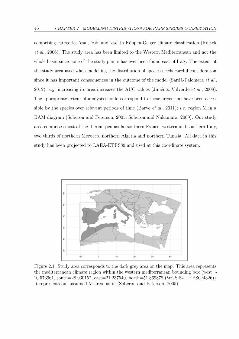
46 CHAPTER 2. MODELLING DISTRIBUTIONS FOR RARE SPECIES CONSERVATION
comprising categories 'csa', 'csb' and 'csc' in K•oppen-Geiger climate classi�cation (Kottek
et al., 2006). The study area has been limited to the Western Mediterranean and not the
whole basin since none of the study plants has ever been found east of Italy. The extent of
the study area used when modelling the distribution of species needs careful consideration
since it has important consequences in the outcome of the model (Sard�a-Palomera et al.,
2012); e.g. increasing its area increases the AUC values (Jim�enez-Valverde et al., 2008).
The appropriate extent of analysis should correspond to those areas that have been acces-
sible by the species over relevant periods of time (Barve et al., 2011); i.e. region M in a
BAM diagram (Sober�on and Peterson, 2005; Sober�on and Nakamura, 2009). Our study
area comprises most of the Iberian peninsula, southern France, western and southern Italy,
two thirds of northern Morocco, northern Algeria and northern Tunisia. All data in this
study has been projected to LAEA-ETRS89 and used at this coordinate system.
Figure 2.1: Study area corresponds to the dark grey area on the map. This area representsthe mediterranean climate region within the western mediterranean bounding box (west=-10.573961, south=28.930152, east=21.237540, north=51.369878 (WGS 84 { EPSG:4326)).It represents our assumed M area, as in (Sober�on and Peterson, 2005)
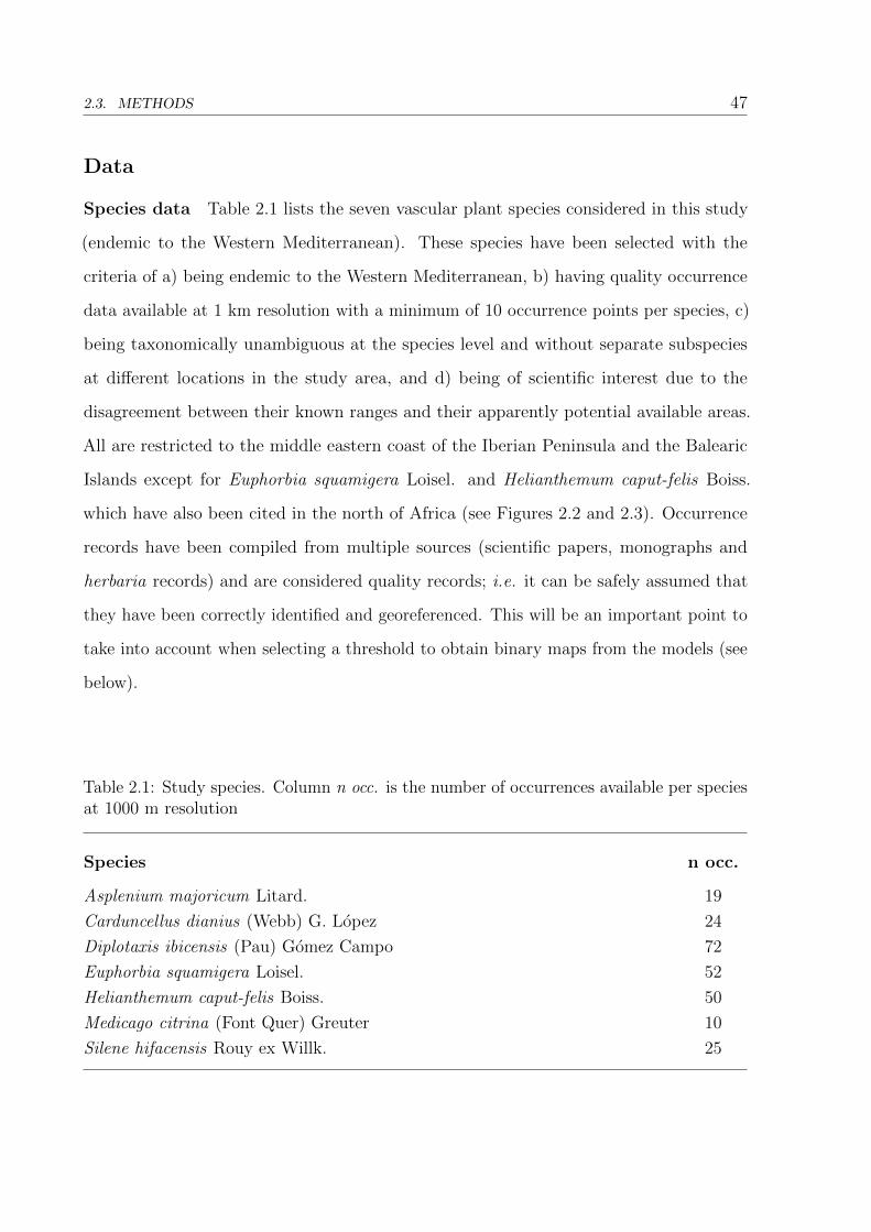
2.3. METHODS 47
Data
Species data Table 2.1 lists the seven vascular plant species considered in this study
(endemic to the Western Mediterranean). These species have been selected with the
criteria of a) being endemic to the Western Mediterranean, b) having quality occurrence
data available at 1 km resolution with a minimum of 10 occurrence points per species, c)
being taxonomically unambiguous at the species level and without separate subspecies
at di�erent locations in the study area, and d) being of scienti�c interest due to the
disagreement between their known ranges and their apparently potential available areas.
All are restricted to the middle eastern coast of the Iberian Peninsula and the Balearic
Islands except for Euphorbia squamigera Loisel. and Helianthemum caput-felis Boiss.
which have also been cited in the north of Africa (see Figures 2.2 and 2.3). Occurrence
records have been compiled from multiple sources (scienti�c papers, monographs and
herbaria records) and are considered quality records; i.e. it can be safely assumed that
they have been correctly identi�ed and georeferenced. This will be an important point to
take into account when selecting a threshold to obtain binary maps from the models (see
below).
Table 2.1: Study species. Column n occ. is the number of occurrences available per speciesat 1000 m resolution
Species n occ.
Asplenium majoricum Litard. 19
Carduncellus dianius (Webb) G. L�opez 24
Diplotaxis ibicensis (Pau) G�omez Campo 72
Euphorbia squamigera Loisel. 52
Helianthemum caput-felis Boiss. 50
Medicago citrina (Font Quer) Greuter 10
Silene hifacensis Rouy ex Willk. 25

48 CHAPTER 2. MODELLING DISTRIBUTIONS FOR RARE SPECIES CONSERVATION
Environmental predictors We used the set of 19 bioclimatic variables which represent
a combination of annual trends, seasonality and extreme conditions relevant to species
physiological tolerances (Nix, 1986). We added two more variables: distance to the
coast (these plants are clearly distributed along the coast) and soil pH (presence of these
plants seems to be clearly associated with soil pH) (see table 2). Bioclimatic variables
were obtained from the WorldClim database (Hijmans et al., 2005). pH was prepared
by completing the information provided by the European Soil Database (European Soil
Data Centre, 2012) with information provided by the Harmonized World Soil Database
(FAO/IIASA/ISRIC/ISSCAS/JRC, 2012) for the North of Africa. Distance to the coast
was computed using boundaries extracted from GADM database of Global Administrative
Areas (http://www.gadm.org). Since the aim of this study is not explanatory but predictive
and since collinearity does not seem to a�ect predictive performance when using Maxent
(Kuemmerle et al., 2010), all predictors were kept when modelling and no collinearity
analysis between predictors was done. All environmental predictors were prepared in the
ETRS89 / ETRS-LAEA coordinate system (EPSG:3035) at 1000 m resolution.
Solving resolution issues These endemic species have restricted narrow coastal ranges,
which means that some records are very close to the coastline. Due to resolution issues,
some of these records may fall in no-data pixels of the environmental set of predictors, that
is, they are 'sea-pixels' in the predictors' layers. For each predictor variable we assigned
the value of their closest neighbour to these no-data pixels or the mean value if more than
one neighbour was present. This allowed us to keep all occurrence records for modelling,
instead of having to discard valid occurrence points from already scarce data.
Species distribution modelling
Modelling approach Occurrence records for these rare endemics are presence-only
and scarce. Techniques for dealing with such conditions have been developed in the last
few years. One of such techniques is maximum entropy modelling (Maxent), which has

2.3. METHODS 49
Table 2.2: Set of environmental predictors used. All predictors were projected to ETRS89/ ETRS-LAEA (EPSG: 3035) coordinate system
Bioclimatic variables
Annual mean temperature
Minimum temperature of the coldest month
Mean temperature of the coldest year quarter
Mean temperature of the warmest year quarter
Mean temperature of the wettest year quarter
Mean temperature of the driest year quarter
Maximum temperature of the warmest month
Annual mean precipitation
Precipitation of the coldest year quarter
Precipitation of the driest month
Precipitation of the driest year quarter
Precipitation of the warmest year quarter
Precipitation of the wettest month
Precipitation of the wettest year quarter
Annual temperature range
Mean temperature diurnal range
Isothermality
Temperature seasonality
Precipitation seasonality
Mean solar radiation of the least radiated quarter
Mean solar radiation of the most radiated quarter
Soil variables
pH
Physical variables
Distance to coast
been proved valid in conservation assessment for modelling species distributions with
scarce presence-only data (Phillips et al., 2006; Elith et al., 2006; Pearson et al., 2007;
Elith et al., 2011; Rebelo and Jones, 2010). We used Maxent software (version 3.3.3k,
http://www.cs.princeton.edu/ schapire/maxent/). MaxEnt estimates the distribution of
maximum entropy constrained in such a way that expected values for predictor variables

50 CHAPTER 2. MODELLING DISTRIBUTIONS FOR RARE SPECIES CONSERVATION
match their empirical average. Its logistic output can be interpreted as the relative
environmental suitability of each pixel in relation to the background of the study area
(Phillips et al., 2006; Phillips and Dud��k, 2008). Models were run using the default set of
parameters of the software and using the whole set of environmental predictors (Table
3.2).
Dealing with spatial autocorrelation Spatial autocorrelation (SAC) needs to be
taken into account in order to avoid in ation of accuracy measures (Veloz, 2009). We used
a preventive approach to SAC avoidance by preparing several 'a priori' autocorrelation
treatments as in Marcer et al. (2012). For each species, we prepared four di�erent sets of
records corresponding to minimum euclidean distances (1500m, 3000m, 4500m, 6000m),
�ve sets corresponding to minimum environmental distances according to the Gower metric
(Gower, 1971) (0.025, 0.050, 0.75, 0.1, 0.125) and one set with all occurrence records.
Residual SAC (observed occurrence minus probability of occurrence) was then measured
as in De Marco Jr et al. (2008); Nu~nez and Medley (2011); V�aclav��k and Meentemeyer
(2012); Marcer et al. (2012) using Monte-Carlo simulation of Moran's I autocorrelation
coe�cient using package spdep in R (Bivand et al., 2011). All models with signi�cant
residual SAC were discarded (25 out of 70).
Model evaluation and selection We validated the remaining 45 models by partly
following the methodology described in Pearson et al. (2007). When the number of
occurrences was low (in our case, < 25) it was feasible to calculate the 2N possible D
statistics (as proposed by Pearson et al. (2007)). In these cases, we used the software
prepared by those authors and which they made available as supplementary information in
their work. On the other hand, for higher number of occurrences we designed an alternative
test. We split the number of occurrences, N , into M groups with the an equal number of
elements, NM
. Although this approach does not work when N is a prime number, there
was no such case. Next, we implemented a jackknife "leave- NM
-out" procedure whereby
M occurrence maps were computed with the Maxent algorithm by leaving NM
occurrence
data points out each time. We de�ned the test criterion D∗ simply as the sum of all
2.3. METHODS 51
successes, where success for each map was de�ned as the number of points that were
correctly predicted:
D∗ =M∑i=1
xi where x 2 0, ..., NM
Notice that, in this case, we abandoned the weighting strategy of Pearson et al. (2007) for
the sake of simpli�cation. All possible simulated D∗ values were calculated by assuming
that each xi could take on any value between 0 and NM
and we checked whether D∗simulated �
D∗observed. When this inequality was true we added the probability of obtaining the simulated
D∗ value as de�ned by:
P =M∏i=1
B(xi,NM, pi)
where B is the probability mass function of a binomially distributed random variable and
pi is the proportion of the study area that was predicted by the corresponding map, as in
Pearson et al. (2007). For the sake of comparison between our proposed methodology and
that of Pearson et al. (2007) we calculated the D* index and its associated probability for
one species and for all possible number of groups M, and veri�ed whether all resulting
probabilities were similar.
Of all accepted models and for each species, we chose the model with the highest
success rate when considering all test points from all cross-validation folds; i.e. number of
correctly classi�ed test points divided by the total number of test points. See Table 2.3 (we
used a threshold-dependent validation, test AUC of Maxent is only given for informative
purposes). Finally, we run again the chosen models with the whole set of occurrences to
obtain the �nal suitability map. Maps of these models can be found in Appendix A.
Geographic range
Potential range maps can be derived from species distribution models by applying
a cut-o� threshold value to determine suitable and unsuitable areas. EOO and AOO
are both valid measures of range size under IUCN criteria for the red listing of species.
EOO is "the area contained within the shortest continuous imaginary boundary which can

52 CHAPTER 2. MODELLING DISTRIBUTIONS FOR RARE SPECIES CONSERVATION
be drawn to encompass all the known, inferred or projected sites of present occurrence
of a taxon, excluding cases of vagrancy" while AOO is "the area within its 'extent of
occurrence' which is occupied by a taxon, excluding cases of vagrancy" (IUCN, 2001).
Measures of overall potential range area, EOO and AOO are given in Table 2.4.
Extent of occurrence (EOO) For each species, EOO was computed as the area
resulting from applying the convex hull method (package 'dismo' in R; Hijmans et al.
(2012)) to all available occurrence points for each species. The area occupied by clearly
unsuitable habitat (in our case, the sea) inside the hull was subtracted from the total.
This method is acknowledged by IUCN as a valid measure of the EOO (IUCN, 2001).
Threshold selection In order to calculate AOO we need binary maps which can be
obtained from continuous probability models by setting a threshold value above which the
location is considered suitable. Since our occurrence data are accurate and reliable (for
correct species identi�cation and georeferencing) we used the MTP (Minimum Training
Presence) value as threshold. MTP is the logistic threshold that results in inclusion of
all training presences. This also ensures a zero omission rate, which is a desired outcome
when trying to de�ne suitable areas for species of conservation interest with limited ranges.
Also, MTP can easily be argued ecologically since it includes all sites that are at least as
suitable as those where the species has been recorded as present (Pearson et al., 2007).
Since our aim is to calculate the suitable area for the species, the inclusion of all areas
with a probability value above MTP seems a sensible decision. We converted the chosen
models (Table 3) into binary maps by setting all values below MTP as zero and all values
equal or above MTP as one (see Appendix A and B).
Area of occupancy We used R (R Core Team, 2012) packages raster (Hijmans and
van Etten, 2012) and dismo (Hijmans et al., 2012) to calculate the total suitable area of
the species (we refer to it as PSA (Potentially Suitable Area)) and the Area of Occupancy
(AOO) de�ned as the PSA within the EOO (Extent of Occurrence). All areas were
calculated at 1000 m resolution but, for AOO, we also calculated it at 2000 m resolution in
order to follow the guidelines given by IUCN (IUCN Standards and Petitions Subcomittee,

2.4. RESULTS 53
2011) for assessing the conservation status of a species.
Assessing the protection status of species
We prepared a raster layer of protected sites by combining information from Natura 2000
boundaries (European Environment Agency, http://www.eea.europa.eu) for the European
part of our study area with information from the World Database on Protected Areas
(IUCN and UNEP, 2009) for the African part of it. The protection layer was obtained at 100
m resolution. We changed the resolution of our binary maps of suitability/unsuitability to
match the resolution of the protected areas layer. Then, we calculated the percentage of 100
m cells of PSA, EOO and AOO that were covered by protected areas as provided in Table
2.5. In the table shown, an indication of the conservation status of each species according
to criteria B1 and B2 of IUCN is given (IUCN Standards and Petitions Subcomittee,
2011).
2.4 Results
Distribution models and range maps for seven narrow-range endemic plant species of
the western Mediterranean have been provided (see Figure 2.2, Figure 2.3 and Appendix
A. For these species, the authors only have evidence of a former study on Helianthemum
caput-felis (Zaragoz�� et al., 2012) dealing only with the analysis of open source software for
AOO calculation. Table 2.3 shows the best models per species (a �gure for each model is
available in Appendix A). Except for Medicago citrina, all species needed some sort of SAC
treatment (two euclidean and four environmental) which implied losing some occurrences
for modelling (2.4). After SAC treatment, occurrence records diminished from as low
as 42% for Euphorbia squamigera to as high as 64% for Silene hifacensis. Occurrence
records available for modelling ranged from as low as 9 (Asplenium majoricum and Silene
hifacensis) up to 40 (Diplotaxis ibicensis). Success rates for classi�cation of test points
were very high, ranging from 0.889 (Asplenium majoricum and Silene hifacensis) to 0.975
(Diplotaxis ibicensis). Test AUC is provided only for informative purposes and ranges
from 0.968 to 0.999.

54 CHAPTER 2. MODELLING DISTRIBUTIONS FOR RARE SPECIES CONSERVATION
We tested how the proposed D* described above, which we applied when the number
of cases was � 25, performed when compared to the methodology in Pearson et al. (2007).
We computed D* for the Helianthemum caput-felis dataset (24 cases, see Table 3) for
M=2, 4, 6 and 8 groups. The corresponding probability p was in all cases larger than the
case where M=24, although always very small and signi�cative. That is, D* performs in
our test more conservatively than the original D in Pearson et al. (2007), although the
di�erences are always very small and negligible within the context of our study.
Table 2.3: A list of the �nally chosen models selected by having the highest success rate,alphabetically ordered. Column Test AUC is given only for informative purposes. ColumnSAC treatment indicates which of the corresponding treatments led to the �nally chosenmodel. Column Nr. occ. indicates the number of occurrences used per species. ColumnMTP is the Minimum Training Presence threshold used when generating the binary maps
Species Nr. occ. SAC treatment Success rate Test AUC MTP
Asplenium majoricum 9 gower (0.125) 0.889 0.968 0.2982
Carduncellus dianius 11 euclidean (1500 m) 0.909 0.998 0.2185
Diplotaxis ibicensis 40 gower (0.025) 0.975 0.998 0.0764
Euphorbia squamigera 30 gower (0.075) 0.933 0.882 0.2131
Helianthemum caput-felis 24 gower (0.025) 0.917 0.997 0.1543
Medicago citrina 10 none 0.900 0.999 0.5829
Silene hifacensis 9 euclidean (4500 m) 0.889 0.997 0.3799
Table 2.4 shows the PSA, EOO, AOO calculated at 1000 m resolution, AOO calculated
at 2000 m resolution and the corresponding proportions of EOO with respect to PSA and
AOO with respect to both PSA and EOO. These proportions serve as an index of how
close the species distribution is to its potential range and to its extent of occurrence. This
can be seen in Figures 2.2 and 2.3. Euphorbia squamigera appears to be the species which
uses more of its potential range (71.3%) and Carduncellus dianius is the one which is
more narrowly distributed in relation to its PSA (only 3.0% of its PSA is EOO). As for
the relation of AOO to EOO, three species (Asplenium majoricum, Carduncellus dianius
and Silene hifacensis) have a suitable area of 88% or more of their EOO, three of them
(Diplotaxis ibicensis, Helianthemum caput-felis and Medicago citrina) appear to have
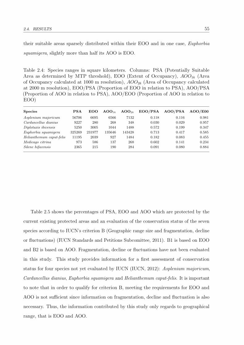
2.4. RESULTS 55
their suitable areas sparsely distributed within their EOO and in one case, Euphorbia
squamigera, slightly more than half its AOO is EOO.
Table 2.4: Species ranges in square kilometers. Columns: PSA (Potentially SuitableArea as determined by MTP threshold), EOO (Extent of Occupancy), AOO1k (Areaof Occupancy calculated at 1000 m resolution), AOO2k (Area of Occupancy calculatedat 2000 m resolution), EOO/PSA (Proportion of EOO in relation to PSA), AOO/PSA(Proportion of AOO in relation to PSA), AOO/EOO (Proportion of AOO in relation toEOO)
Species PSA EOO AOO1k AOO2k EOO/PSA AOO/PSA AOO/E00
Asplenium majoricum 56706 6695 6566 7132 0.118 0.116 0.981
Carduncellus dianius 9227 280 268 348 0.030 0.029 0.957
Diplotaxis ibicensis 5250 3005 1044 1488 0.572 0.199 0.347
Euphorbia squamigera 325269 231977 135646 143428 0.713 0.417 0.585
Helianthemum caput-felis 11195 2039 927 1484 0.182 0.083 0.455
Medicago citrina 973 586 137 268 0.602 0.141 0.234
Silene hifacensis 2365 215 190 284 0.091 0.080 0.884
Table 2.5 shows the percentages of PSA, EOO and AOO which are protected by the
current existing protected areas and an evaluation of the conservation status of the seven
species according to IUCN's criterion B (Geographic range size and fragmentation, decline
or uctuations) (IUCN Standards and Petitions Subcomittee, 2011). B1 is based on EOO
and B2 is based on AOO. Fragmentation, decline or uctuations have not been evaluated
in this study. This study provides information for a �rst assessment of conservation
status for four species not yet evaluated by IUCN (IUCN, 2012): Asplenium majoricum,
Carduncellus dianius, Euphorbia squamigera and Helianthemum caput-felis. It is important
to note that in order to qualify for criterion B, meeting the requirements for EOO and
AOO is not su�cient since information on fragmentation, decline and uctuation is also
necessary. Thus, the information contributed by this study only regards to geographical
range, that is EOO and AOO.
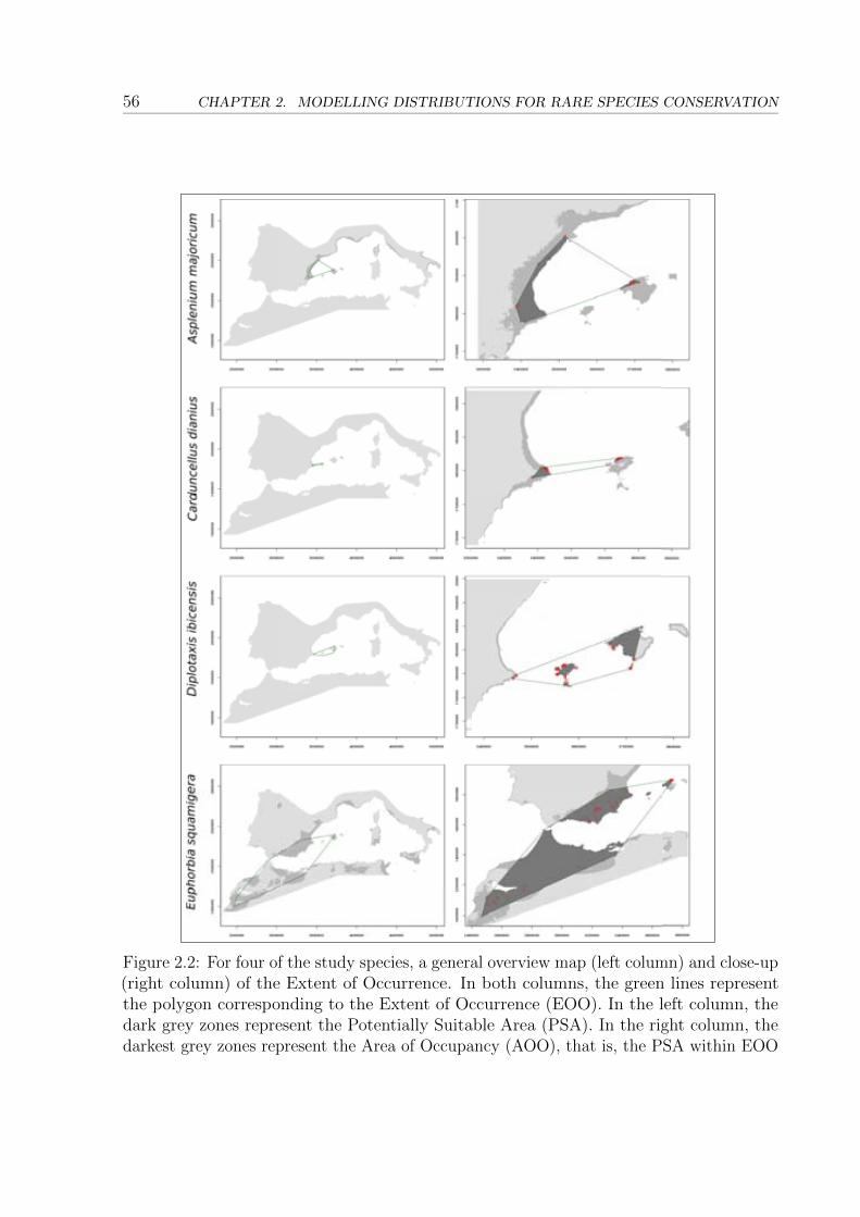
56 CHAPTER 2. MODELLING DISTRIBUTIONS FOR RARE SPECIES CONSERVATION
Figure 2.2: For four of the study species, a general overview map (left column) and close-up(right column) of the Extent of Occurrence. In both columns, the green lines representthe polygon corresponding to the Extent of Occurrence (EOO). In the left column, thedark grey zones represent the Potentially Suitable Area (PSA). In the right column, thedarkest grey zones represent the Area of Occupancy (AOO), that is, the PSA within EOO
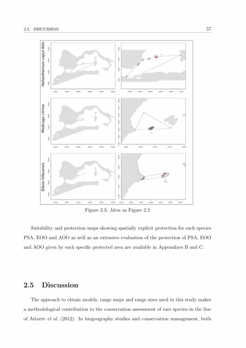
2.5. DISCUSSION 57
Figure 2.3: Idem as Figure 2.2
Suitability and protection maps showing spatially explicit protection for each species
PSA, EOO and AOO as well as an extensive evaluation of the protection of PSA, EOO
and AOO given by each specific protected area are available in Appendixes B and C.
2.5 Discussion
The approach to obtain models, range maps and range sizes used in this study makes
a methodological contribution to the conservation assessment of rare species in the line
of Attorre et al. (2012). In biogeography studies and conservation management, both

58 CHAPTER 2. MODELLING DISTRIBUTIONS FOR RARE SPECIES CONSERVATION
Table 2.5: Species conservation status and protection. Column PSAPR indicates thepercentage of PSA that is protected, column EOOPR indicates the percentage of EOOthat is protected and AOOPR the percentage of AOO that is protected. Columns IUCNB1
and IUCNB2 indicate the evaluation made by this study for each species according to therange part of criteria B1 (CR: <100 km2, EN: <5000 km2, VU: <20000 km2) and B2 (CR:<10 km2, EN: <500 km2, VU: <2000 km2) of IUCN. Column IUCNCUR indicates thecurrent IUCN assessment (IUCN, 2012). IUCN categories: CR (Critically Endangered),EN (Endangered), VU (Vulnerable), LC (Least Concern), NE (Not Evaluated))
Species PSAPR EOOPR AOOPR IUCNB1 IUCNB2 IUCNCUR
Asplenium majoricum 24.6 22.2 22.4 VU LC NE
Carduncellus dianius 22.8 17.9 17.9 EN EN NE
Diplotaxis ibicensis 23.9 18.4 22.2 EN VU LC
Euphorbia squamigera 19.9 13.0 18.9 LC LC NE
Helianthemum caput-felis 20.3 14.6 27.6 EN VU NE
Medicago citrina 27.9 15.3 24.9 EN EN CR
Silene hifacensis 27.5 22.5 22.9 EN EN EN
realized and potential distributions are of much interest { realized distributions to ensure
conservation and potential distributions as candidate areas for relocation or for discovering
unknown populations (Wilson et al., 2011; Thorn et al., 2009; Peterson et al., 2011).
It is necessary to explicitly distinguish between realized and potential distributions
when modelling species distributions since di�erent methods and data will lead to diferent
outcomes. Both presences and absences are necessary when modelling realized distributions
(Jim�enez-Valverde et al., 2008; Sober�on and Nakamura, 2009; Jim�enez-Valverde, 2012).
Absence data, specially when considering coarse grid data, is very hard to obtain and
justify since absences may be of false origin, i.e. the species is present but has not been
observed (Gu and Swihart, 2004). In our case, only presence data is available and the
outcome of our model should be considered as PSA. The studied species represent a set of
rare species of high conservation interest in a well-surveyed zone for vascular plants at
1000 m resolution. According to experts, for these species, it can be safely assumed that
their occurrence points closely approximate their extent of occurrence (EOO); i.e though
not impossible, it is unlikely that new occurrences will be found outside their current EOO.
Therefore, the PSA which falls inside the EOO can be considered a good approximation
to the AOO of the species.

2.5. DISCUSSION 59
In the case of rare species in well-surveyed areas where their EOO is well-known,
the models resulting from species distribution modelling can be interpreted in terms of
realized and potential distributions. With presence-only data, the potentially suitable
area within EOO is the best approximation we can have to a realized distribution or
AOO. Moreover, when the purpose of these modelling exercises is to generate valuable
information for conservation e�orts the selection of the MTP threshold is an adequate
one to generate binary maps of suitability/unsuitability (Pearson et al., 2007). Therefore,
in these circumstances, the knowledge gained from the modelled current and potential
distribution of the species can be used to assess the conservation of the species by generating
maps and reports of their protection status (see Supplementary Materials).
Conservation can't a�ord to wait until enough information is available for a given species
since we may end up losing the species in the process. It thus becomes necessary to make
the best informed decisions possible at any given moment. Combining expert judgement
with modelling tools can be the best solution at hand. Using this approach, we have
provided valuable conservation and protection assessment status for these seven species.
This protocol can't be considered de�nitive but it can be repeated as new occurrence data
becomes available, specially so in the unlikely case that it enlarges the current known
EOO of the species. One can envisage an information system which uses this protocol and
provides up-to-date conservation assessments for rare species where the PSA, EOO and
AOO are automatically updated.
The species in our study were also selected because they puzzled botanists due to the
fact that their EOO seems very restricted if one considers the apparently available suitable
area that they have at their disposal, i.e. Grinnellian niche. This study contributes to
con�rming and highlighting this fact as can be seen in Table 2.4. The models do show a
much wider suitable area for each of the seven species than the area they actually occupy.
Except for Asplenium majoricum whose dispersion is by anemocory, the other six species
are dispersed by barochory alone (Medicago citrina shows zoocory to a lesser degree).
For these six species, one can argue that their restricted current range compared to their
available suitable area is due to historical phylogeographical reasons as well as to their
60 CHAPTER 2. MODELLING DISTRIBUTIONS FOR RARE SPECIES CONSERVATION
form of dispersal. For Asplenium majoricum this argument does not hold and we should
point to other reasons such as the use of an excessively restricted set of predictor variables.
It may be argued that, except for Asplenium majoricum, the area where the species has
had historical access because of its movement and colonizing capacities, the M region
as in Sober�on and Peterson (2005) and Sober�on and Nakamura (2009), appears to be
their current extent of occurrence. If so, given that some authors argue that the extent of
analysis should correspond to those areas that have been accessible by the species over
relevant periods of time (Barve et al., 2011), further modelling e�orts might be made using
only their EOO or a slightly bu�ered EOO.
For the particular case of Euphorbia squamigera, our model shows a high suitability
index in the Provence zone in France, outside the estimated EOO. It is interesting to
note that the �rst description of this species was done in the area of Toulon (Loiseleur-
Deslongchamps, 1807). However, apart from this �rst citation, the plant has not been
found again, which has always made botanists doubt about it in the �rst place (this is the
reason why we have excluded this presence in our modelling occurrence data) and think
this may be a case of misidenti�cation. Our results lend support for the correctness of this
�rst citation. If it were to be con�rmed, this citation would add to the validity of the PSA
obtained from the models although the EOO and AOO would need to be recalculated.
This also reinforces the fact that these models show PSA rather than realized distributions.
The set of predictor variables used in this study, combined with the lack of absences in
our modelling technique, is not su�cient to restrict the output distribution to the realized
distribution.
Table 2.4 shows the absolute values found in this study for each species' PSA, EOO and
AOO. Interestingly, the EOO of Asplenium majoricum, which is dispersed by anemocory,
represents only about 12% of the available PSA. As stated above, this could be explained
by the lack of appropriate predictor variables in this study. On the other hand, its EOO is
almost covered by its AOO, which can be explained by its dispersal form. However, more
hidden factors seem to play an important role in its distribution since very few occurrences
are available for this area. For the remaining species, which are dispersed by barocory,

2.6. CONCLUSIONS 61
there is a wide span of values of the relation AOO/EOO, from 23.4% to 95.7%. Contrary
to the case of Asplenium majoricum one would expect these values to be low due to their
form of dispersal. Here, there are also hidden factors at play which are outside the scope
of this study, although it does not seem to be the case at present, predation may have
played its role historically.
Species distribution modelling for rare species in well-surveyed areas can provide a
good approximation to species realized and potential distributions. These distributions can
be overlaid with the network of protected areas and give valid assessments of conservation
status and protection. Table 2.5 provides an assessment of the protection given by current
protected areas to each species' PSA, EOO and AOO and valuable information for the
classi�cation of each species according to IUCN categories of threatened species (IUCN
Standards and Petitions Subcomittee, 2011). From a conservation management perspective,
the protected percentage of EOO and AOO can give an indication of how well-covered the
range of the species is by protected areas. Also, the information regarding the presence
of part of the species PSA in each protected area can be of great use should relocation
e�orts be considered for enlarging the current EOO and thus, add to the probability of
the species persistence (a comprehensive list of the protected areas that contain part of
each species PSA is given in Appendix C).
2.6 Conclusions
Species distribution modelling is a valid tool for generating valuable information for
conservation management when dealing with rare species in well-surveyed areas. The use
of well-known EOOs of species with modelled maps of suitability o�ers a way to discern
between an approximation of realized and potential distributions. This paper provides
probability models and range maps for seven rare endemic vascular plants of the western
Mediterranean for the �rst time and a �rst quantitative assessment of their realized and
potential distributional areas, their degree of protection and information useful to assess
their degree of threat.

62 CHAPTER 2. MODELLING DISTRIBUTIONS FOR RARE SPECIES CONSERVATION
Except for one case, the PSAs for the set of studied species are much larger than
their corresponding EOOs. This con�rms the previously existing expert view which was
unsupported by data that these species are much more restricted in range than the area
that appears to be suitable for them. Although not explored in this study, this is probably
due to a combination of historical phylogeographical reasons and to the absence of some
environmental or biotic predictors which could contribute to determine the species' spatial
distribution.
2.7 Acknowledgements
The authors wish to thank Llu��s Brotons for his helpful comments on an earlier
draft which helped to improve the manuscript. This study was supported by project
CONSOLIDER-MONTES (CSD2008-00040) of the Ministerio de Ciencia e Innovaci�on of
the Spanish government. Xavier Pons is recipient of an ICREA Academia Excellence in
research grant 2011-2015.
Chapter 3
Modelling invasive alien species
distributions from digital biodiversity
atlases. Methodological insights for
reconciling data at different scales
This chapter has been published in:
Arnald Marcer, Joan Pino, Xavier Pons, Llu��s Brotons
Diversity and Distributions, Volume 18, Issue 12, December 2012, Pages 1177-1189
doi:10.1111/j.1472-4642.2012.00911.x
63
64 CHAPTER 3. MODELLING IAS DISTRIBUTIONS FROM BIODIVERSITY ATLASES
3.1 Abstract
Aim There is a wealth of information on species occurrences in biodiversity data banks,
albeit presence-only, biased and scarce at the �ne resolutions. Moreover, in biodiversity
conservation �ne-resolution species maps are in need. New techniques for dealing with
this kind of data have been reported to perform well. However, when good coarser scale
data are available, are these �ne-resolution maps robust enough to also explain coarser
distributions ? We present a new methodology for testing this hypothesis and apply it to
invasive alien species (IAS).
Location Catalonia, Spain.
Methods We used species presence records from the Biodiversity data bank of Catalo-
nia to model the distribution of ten IAS which, according to some recent studies, achieve
their maximum distribution in the study area. To overcome problems inherent with the
data, we prepared di�erent correction treatments: three for dealing with bias and �ve for
autocorrelation. We used the MaxEnt algorithm to generate models at 1 km resolution
for each species and treatment. Acceptable models were upscaled to 10 km and validated
against independent 10 km occurrence data.
Results Out of a total of 150 models, 20 gave acceptable results at 1 km resolution
and 12 passed the cross-scale validation test. No apparent pattern emerged which could
serve as a guide on modelling. Only four species gave models that also explained the
distribution at the coarser scale.
Main conclusions Although some techniques may apparently deliver good distribu-
tions maps for species with scarce and biased data, they need to be taken with caution.
When good independent data at a coarser scale are available, cross-scale validation can
help producing more reliable and robust maps. When no independent data are available
for validation, however, new data gathering �eld surveys may be the only option if reliable
�ne-scale resolution maps are needed.
Keywords Invasive alien species, atlas, biodiversity databases, Catalonia, cross-scale
validation, maxent, Spain, species distribution models

3.2. INTRODUCTION 65
3.2 Introduction
For centuries, species occurrences have been recorded in an ad hoc way by natural
historians, museums, scientists and the like in the form of museum specimens, site
inventories, citations in technical and scienti�c literature, etc. (Chapman and Busby,
1994; Chapman, 2005b). In the last two to three decades, both governments and non-
governmental organizations have invested considerable �nancial resources on the digitizing
of these data into digital species distribution atlases and making them publicly available.
Ideally, they should o�er reliable, high quality data which withstands public, scienti�c and
legal scrutiny (Robertson et al., 2010). Such databases represent a wealth of information
on species distribution and an indispensable asset for science and conservation (Funk
and Richardson, 2002; Graham et al., 2004; Suarez and Tsutsui, 2004; Franklin, 2009;
Robertson et al., 2010). However, since these data usually come from opportunistic or ad
hoc sources rather than well-planned surveys, they present some important drawbacks:
they are presence-only in nature, are highly biased and may show spatial agregation
derived from sampling biases. Also, since they are laborously compiled from analog
sources, they are di�cult and costly to georeference and hence, coarser resolutions tend
to dominate (Margules and Pressey, 2000; Pressey, 2004). As a result, most data in this
kind of biodiversity databases are often too coarse for use in conservation planning and
management, where �ne grained maps (i.e. 1 km or better) are needed (McPherson et al.,
2006; Guralnick and Hill, 2009; Niamir et al., 2011).
Planned systematic surveys of species presence and abundance could provide the most
precise, accurate and unbiased information on the spatial distribution of biodiversity.
However, such surveys are expensive to conduct for large regions, even for a single species
(Robertson et al., 2010). Given the current accelerated trend in world-wide biodiversity
loss and the urge for addressing conservation problems, it becomes of utmost importance
to �nd ways and methodologies to make the best use of this already available information
(Newbold, 2010; Venette et al., 2010).
Such databases or atlases of species occurrences still represent a largely untapped

66 CHAPTER 3. MODELLING IAS DISTRIBUTIONS FROM BIODIVERSITY ATLASES
potential of information which can play an important role in conservation biogeography
(Richardson and Whittaker, 2010). Fortunately, in the last few years the community of
species distribution modelling has witnessed the appearance of new tools and methodologies
from the �elds of statistics and arti�cial intelligence which have the potential to address
the problems inherent in these data. Some of these tools have been specially tailored to
model presence-only data even when only few occurrences are available and problems such
as bias and autocorrelation are present. One of such techniques, maximum entropy, has
been judged among the best performers in distribution modelling for such kind of data
(Elith et al., 2006).
In many cases, applying these novel techniques to the scarce �ne-resolution data can
yield distribution maps with high validation scores. The question is whether we can take
advantage of coarser data, which are relatively abundant and for some regions close to
the species true distribution, to further validate these maps and �nd out their reliability.
Having models that explain data at �ne resolutions while being consistent with coarser
resolution data is important (McPherson et al., 2006; Niamir et al., 2011) as it can yield
more robust and reliable distribution maps for conservation.
The existence of databases with such information provides an opportunity to check this
hypothesis. A specially relevant piece of information for conservation which can potentially
be derived from these costly data banks are current and historical distributions of Invasive
Alien Species (IAS).
The spread of IAS, driven mainly by human activities, is increasing worldwide (Butchart
et al., 2010) and pose potential problems not only to native biodiversity but also to economic
development and human well-being (Vitousek et al., 1997; Taylor and Irwin, 2004; Pimentel
et al., 2005; Chytr�y et al., 2009; Pejchar and Mooney, 2009; Py�sek et al., 2010; Vil�a et al.,
2011). Having risk maps representing the potential distribution of IAS is a necessary step
towards e�ective management (Richardson and Whittaker, 2010; Jim�enez-Valverde et al.,
2011). Using all information in species inventories and atlases, coarse and �ne resolution
records, is essential in making the most out of limited �nancial resources (Nielsen et al.,
2008).

3.3. METHODS 67
We test whether fine-resolution maps of IAS can be obtained from existing biodiversity
databases which are robust enough to explain occurrences at different scales held in the
database and, if so, whether a general methodology can be devised. We use different bias
and autocorrelation treatments to deal with problems inherent with such data.
3.3 Methods
Area of study
Catalonia is a region of around 32000 km2 located in the northeastern part of the
Iberian Peninsula (Figure 3.1). It ranges in elevation from 0 to over 3000 m.a.s.l, from the
Mediterranean coast up to the Pyrenees. Its environmental conditions are highly variable
due to its complex location and topography. Although dominated by the mediterranean
climate it also has continental and atlantic influences. Mediterranean and Eurosiberian
biogeographic regions dominate while Subalpine and Alpine types appear in the upper zones
of the Pyrenees. There is a trend of decreasing precipitation and increasing temperature
towards the south (Ninyerola et al., 2000). It is a highly humanized territory, particularly
around the Barcelona metropolitan area. The rest of the region is dominated by forests and
agroforestry mosaics with relatively large human influence although with lower intensity.
Figure 3.1: Study area

68 CHAPTER 3. MODELLING IAS DISTRIBUTIONS FROM BIODIVERSITY ATLASES
Database. As a case study we use the Biodiversity Databank of Catalonia (BDBC,
http://biodiver.bio.ub.es/biocat/) (Font et al., 2009). Catalonia is a region with a rich
history in Botany which is re ected in the holdings of the database. For an area of around
32000 km2, the BDBC contains above 1.5 million of plant species citations from sources
such as scienti�c articles, PhD theses and local oras. Due to historical recording tradition
among botanists and to the cost of obtaining �ner georeferences, most of its data is at
a coarse resolution of 10 km. Catalonia is a well-surveyed region for vascular plants at
10 km resolution. BDBC contains also more than 180000 plant occurrence records at
1 km resolution. The geographical distribution of IAS as re ected by 10 km-resolution
occurrence records in the BDBC can be considered to approximate its true distribution for
our study area (Pino et al., 2005). Therefore, when developing models at �ner resolutions
their geographic distribution should be coherent with the distribution obtained from
mapping the coarser data.
Species data
IAS may violate the assumption made in species distribution modelling (Peterson, 2005)
that species are at equilibrium with their environment (Austin, 2002; Ara�ujo and Pearson,
2005; De Marco Jr et al., 2008); i.e. they may not realize their full range (Zimmermann
et al., 2010; V�aclav��k and Meentemeyer, 2012). According to some studies (Williamson
et al., 2009; Gass�o et al., 2010), neophytes reach their maximum range around 150 years
since their introduction in the Iberian peninsula. We used this criterion (more than 150
years since introduction) for the selection of IAS species, in addition to availability of data
at 1 km resolution. The selection resulted in the 10 species shown in Table 3.1 (see also
Appendix D). Of these, four of them are included in the list of DAISIE's one-hundred
worst invaders in Europe (DAISIE, 2011): Ailanthus altissima, Opuntia ficus-indica, Oxalis
pes-caprae and Robinia pseudoacacia.
Data independence across scales. Occurrence data at di�erent resolutions in biodi-
versity atlases may not be independent; i.e. occurrence records at coarser resolutions may
have their origin in records at �ner resolutions. In order to overcome this problem we

3.3. METHODS 69
Table 3.1: List of selected IAS for modelling
Species Abrv. 1kma 10kmb Intrc Yrsd
Agave americana L. aga 20 124 XVIth 411
Ailanthus altissima (P. Mill.) Swingle aia 43 213 1818 192
Amaranthus albus L. ama 29 194 1861 149
Conyza canadiensis (L.) Cronquist coc 73 307 1784 226
Datura stramonium L. das 31 230 XVIth 411
Oenothera biennis L. oeb 55 80 1848 162
Opuntia ficus-indica (L.) P. Mill. opf 13 102 XVIth 411
Oxalis pes-caprae L. oxp 12 41 1850 160
Robinia pseudoacacia L. rop 66 257 XVIIIth 211
Xanthium spinosum L. xas 56 252 XVIIIth 211
aNumber of 1 km occurrencesbNumber of 10 km occurrencescIntroduction datedNumber of years since introduction (conservative estimate)
only accepted 10 km squares which had at least one citation more per species than the
number of 1 km citations contained therein; i.e. there is at least one 10 km occurrence
record which is independent from 1 km data. This procedure also allowed us to use all
occurrences records at 1 km resolution.
Environmental data.
We used 19 bioclimatic variables (Nix, 1986) (Table 3.2) which represent a combination
of annual trends, seasonality and extreme conditions relevant to species physiological
tolerances. We added two more variables regarding radiation (mean radiation of the least
radiated quarter and mean radiation of the most radiated quarter) and three more variables
that may partially explain distribution of IAS (distance to main harbours, distance to
the coast and degree of anthropization) (Brooks, 2007; Vicente et al., 2010) (See Table
3.2). We calculated the bioclimatic variables using the Digital Climatic Atlas of Catalonia
(DCAC) (Ninyerola et al., 2000) which holds monthly data on temperature, precipitation
and radiation for the whole of Catalonia. We calculated the degree of anthropization using
the Land Cover Map of Catalonia (CREAF - Centre for Ecological Research and Forestry
70 CHAPTER 3. MODELLING IAS DISTRIBUTIONS FROM BIODIVERSITY ATLASES
Applications, 2009; Ib�a~nez and Burriel, 2010). Each land cover category was assigned a
value between one (least anthropization) and �ve (most anthropization) (Table 3.2). Then,
to represent the degree of anthropization we calculated a weighted average scaled between
0 and 100 for each 1 km square grid.
Since our goal is to predict species distributions rather than discerning which factors
a�ect their distribution, all predictors were used for modelling each species. Extracting
collinearity from the model was not necessary. Though it can hinder model interpretation,
it does not a�ect Maxent predictive performance (Kuemmerle et al., 2010).
Species distribution modelling
Modelling involved a �ve-step process as shown in Figure 3.2. In the �rst step, we
modelled the species distribution at the �ner resolution of 1 km following the methodology
described in Case 1 (Elith et al., 2011). These authors use di�erent alternative background
scenarios to account for bias, and cross-validation techniques to validate models developed
with presence-only data of Banksia prionotes from an atlas database. Accounting for
bias and autocorrelation is an important issue in species distribution modelling, specially
in presence-only models (Legendre, 1993; Legendre et al., 2002; Segurado et al., 2006;
Phillips et al., 2009; Newbold, 2010; Merckx et al., 2011). Since we expect �ne-grained
casually-collected data to show a number of biases, we included three bias correction
treatments and �ve spatial autocorrelation correction treatments (see below) to evaluate
the potential of these data to derive ecologically sound species distribution models.
This resulted in a total of 15 models per species. In a second step, only those models
with an AUC (area under the curve) � 0.7 not showing residual spatial autocorrelation
were selected. In a third step, these selected models were upscaled to a coarser resolution
of 10 km using a probabilistic model (see Equation 3.1). In step four, upscaled models
were validated against the independent 10 km dataset and only those with an AUC � 0.7
at 10 km resolution (AUC10k) were selected. Therefore, their originating �ne-scale models
were, among the previously selected ones, the ones which showed acceptable predictions
at both scales. Finally, in step �ve, if more than one �ne-scale model per species had
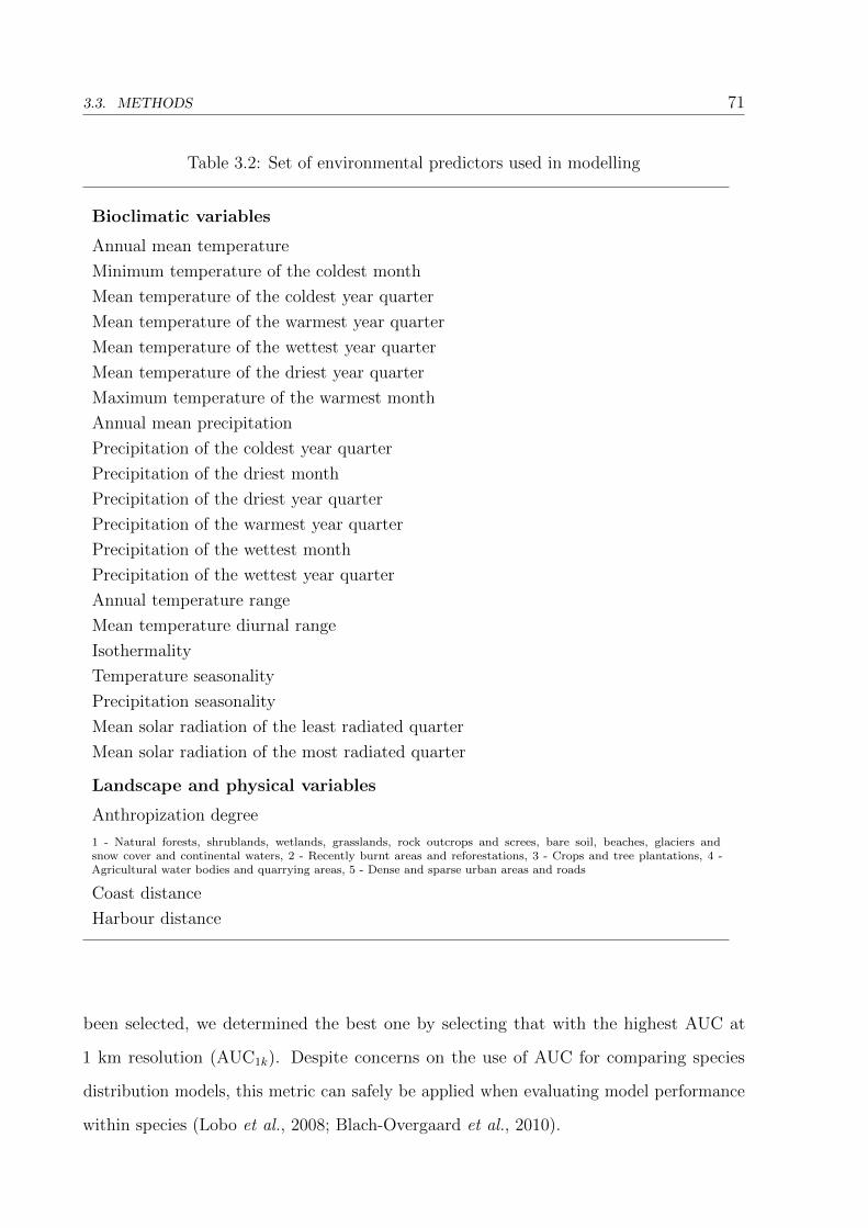
3.3. METHODS 71
Table 3.2: Set of environmental predictors used in modelling
Bioclimatic variables
Annual mean temperature
Minimum temperature of the coldest month
Mean temperature of the coldest year quarter
Mean temperature of the warmest year quarter
Mean temperature of the wettest year quarter
Mean temperature of the driest year quarter
Maximum temperature of the warmest month
Annual mean precipitation
Precipitation of the coldest year quarter
Precipitation of the driest month
Precipitation of the driest year quarter
Precipitation of the warmest year quarter
Precipitation of the wettest month
Precipitation of the wettest year quarter
Annual temperature range
Mean temperature diurnal range
Isothermality
Temperature seasonality
Precipitation seasonality
Mean solar radiation of the least radiated quarter
Mean solar radiation of the most radiated quarter
Landscape and physical variables
Anthropization degree
1 - Natural forests, shrublands, wetlands, grasslands, rock outcrops and screes, bare soil, beaches, glaciers andsnow cover and continental waters, 2 - Recently burnt areas and reforestations, 3 - Crops and tree plantations, 4 -Agricultural water bodies and quarrying areas, 5 - Dense and sparse urban areas and roads
Coast distance
Harbour distance
been selected, we determined the best one by selecting that with the highest AUC at
1 km resolution (AUC1k). Despite concerns on the use of AUC for comparing species
distribution models, this metric can safely be applied when evaluating model performance
within species (Lobo et al., 2008; Blach-Overgaard et al., 2010).

72 CHAPTER 3. MODELLING IAS DISTRIBUTIONS FROM BIODIVERSITY ATLASES
Figure 3.2: Outline for the proposed modelling workflow. Step one corresponds to themodelling of each species at 1 km resolution with three different bias treatments and fivedifferent autocorrelation treatments, which gives a total of 15 models per species. In Steptwo, we check for residual autocorrelation, calculate the AUC and select only those modelswith no residual spatial autocorrelation and with an AUC ≥0.7. In Step three, previouslyselected models are upscaled to 10 km resolution by probabilistic calculations. In Stepfour, a ROC analysis is performed using independent data at 10 km resolution. Modelswith an AUC ≥0.7 tell us which models at 1 km resolution are accepted. Finally, in Stepfive, if more than one model per species at 1 km resolution has been accepted, we definethe best model as the one which has the maximum AUC1k.

3.3. METHODS 73
Bias correction treatments Background samples should be chosen to re ect the
spatial bias and thus, to minimize the e�ects of bias in the data (Phillips et al., 2009;
Veloz, 2009; Elith et al., 2011). We prepared three di�erent background scenarios: a) the
entire study area (coded as 'whole area'), b) 1 km-squares with presence of vascular plants
citations (coded as 'vasculars1k') and c) 1-km squares with presence of IAS citations
(coded as 'invasive1k'). See Table 3.3.
Autocorrelation correction treatments Spatial autocorrelation may falsely in ate
AUC measures for species distribution models with presence-only data (Segurado et al.,
2006; Veloz, 2009) and environmental autocorrelation may have the same e�ects. There is
no established methodology for accounting for spatial autocorrelation when dealing with
presence-only data (Dormann et al., 2007). Autoregressive models are not applicable since
both presence and absence data would be needed (Allouche et al., 2008). We used an
approach a priori similar to (Segurado et al., 2006; Pearson et al., 2007) which consisted
in �ltering occurrences by setting a minimum spatial and environmental distance between
them and then checking for residual autocorrelation. We prepared �ve treatments for
modelling each species. The �rst implied including all available presences without �ltering
them. The second and third involved randomly �ltering and selecting occurrences so
that any occurrence were at least at a spatial distance of 2830 m (two 1 km squares)
and 4250 m (three 1 km squares) from each other, respectively. For the fourth and
�fth treatment we used a minimum multivariate environmental distance based on the
Gower's distance index with values 0.05 and 0.1, respectively (higher values resulted in
an excessive reduction in occurrences). Models were then checked for signi�cant residual
autocorrelation (observed occurrence minus probability of occurrence as in (De Marco
Jr et al., 2008; Nu~nez and Medley, 2011; V�aclav��k et al., 2012)) by using Monte-Carlo
simulation of Moran's I autocorrelation coe�cient using package spdep in R (Bivand et al.,
2011). Only those models with a pvalue � 0.05 were accepted (as shown in Table 3.3).
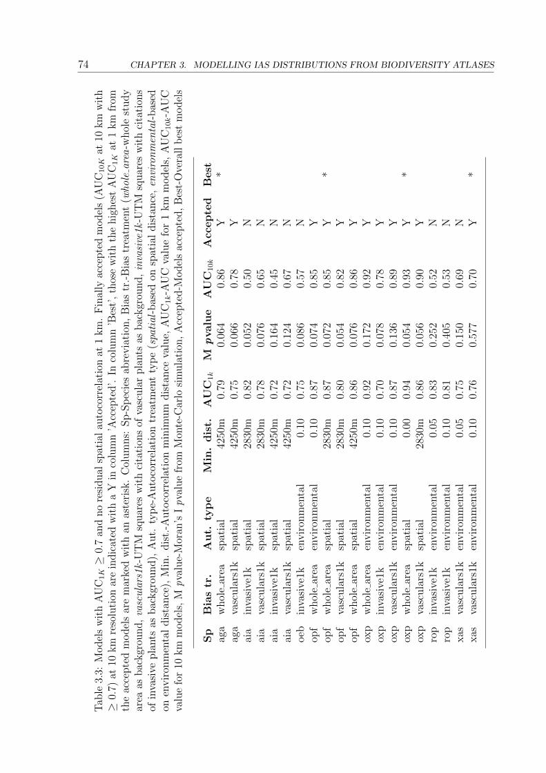
74 CHAPTER 3. MODELLING IAS DISTRIBUTIONS FROM BIODIVERSITY ATLASES
Tab
le3.
3:M
od
els
wit
hA
UC
1K�
0.7
and
no
resi
du
alsp
atia
lau
toco
rrel
atio
nat
1km
.F
inal
lyac
cep
ted
mod
els
(AU
C10K
at10
km
wit
h�
0.7)
at10
km
reso
luti
onar
ein
dic
ated
wit
ha
Yin
colu
mn
'Acc
epte
d'.
Inco
lum
n'B
est'
,th
ose
wit
hth
eh
igh
est
AU
C1K
at1
km
from
the
acce
pte
dm
odel
sar
em
arke
dw
ith
anas
teri
sk.
Col
um
ns:
Sp-S
pec
ies
abre
via
tion
,B
ias
tr.-
Bia
str
eatm
ent
(who
lear
ea-w
hol
est
ud
yar
eaas
bac
kgr
oun
d,
vasc
ula
rs1k
-UT
Msq
uar
esw
ith
cita
tion
sof
vasc
ula
rp
lants
asb
ackgr
oun
d,
inva
sive
1k-U
TM
squ
ares
wit
hci
tati
ons
ofin
vasi
vepla
nts
asbac
kgr
ound),
Aut.
typ
e-A
uto
corr
elat
ion
trea
tmen
tty
pe
(spa
tial
-bas
edon
spat
ial
dis
tan
ce,
envi
ron
men
tal-
bas
edon
envir
onm
enta
ld
ista
nce
),M
in.
dis
t.-A
uto
corr
elat
ion
min
imu
md
ista
nce
valu
e,A
UC
1k-A
UC
valu
efo
r1
km
mod
els,
AU
C10k-A
UC
valu
efo
r10
km
mod
els,
Mp
valu
e-M
oran
'sI
pva
lue
from
Mon
te-C
arlo
sim
ula
tion
,A
ccep
ted
-Mod
els
acce
pte
d,
Bes
t-O
vera
llb
est
mod
els
Sp
Bia
str
.A
ut.
typ
eM
in.
dis
t.A
UC
1k
Mp
valu
eA
UC
10k
Acc
epte
dB
est
aga
whol
ear
easp
atia
l42
50m
0.79
0.06
40.
86Y
*ag
ava
scula
rs1k
spat
ial
4250
m0.
750.
066
0.78
Yai
ain
vasi
ve1k
spat
ial
2830
m0.
820.
052
0.50
Nai
ava
scula
rs1k
spat
ial
2830
m0.
780.
076
0.65
Nai
ain
vasi
ve1k
spat
ial
4250
m0.
720.
164
0.45
Nai
ava
scula
rs1k
spat
ial
4250
m0.
720.
124
0.67
Noeb
inva
sive
1ken
vir
onm
enta
l0.
100.
750.
086
0.57
Nop
fw
hol
ear
eaen
vir
onm
enta
l0.
100.
870.
074
0.85
Yop
fw
hol
ear
easp
atia
l28
30m
0.87
0.07
20.
85Y
*op
fva
scula
rs1k
spat
ial
2830
m0.
800.
054
0.82
Yop
fw
hol
ear
easp
atia
l42
50m
0.86
0.07
60.
86Y
oxp
whol
ear
eaen
vir
onm
enta
l0.
100.
920.
172
0.92
Yox
pin
vasi
ve1k
envir
onm
enta
l0.
100.
700.
078
0.78
Yox
pva
scula
rs1k
envir
onm
enta
l0.
100.
870.
136
0.89
Yox
pw
hol
ear
easp
atia
l0.
000.
940.
054
0.93
Y*
oxp
vasc
ula
rs1k
spat
ial
2830
m0.
860.
056
0.90
Yro
pin
vasi
ve1k
envir
onm
enta
l0.
050.
830.
252
0.52
Nro
pin
vasi
ve1k
envir
onm
enta
l0.
100.
810.
405
0.53
Nxas
vasc
ula
rs1k
envir
onm
enta
l0.
050.
750.
150
0.69
Nxas
vasc
ula
rs1k
envir
onm
enta
l0.
100.
760.
577
0.70
Y*
3.3. METHODS 75
Modelling and validation at 1 km resolution. We used MaxEnt software, version
3.3.3e, (Phillips et al., 2006; Phillips and Dud��k, 2008). MaxEnt is a presence-background
modelling tool based on the maximum entropy principle. There is a wide agreement
among the species distribution modelling community in considering it the best available
tool for presence-only data, even when only a limited number of occurrence records is
available (Elith et al., 2006; Hernandez et al., 2006; Phillips and Dud��k, 2008; Wisz et al.,
2008; Elith and Graham, 2009; Thorn et al., 2009; Costa et al., 2010) and with bias
present (Rebelo and Jones, 2010). MaxEnt estimates the distribution of maximum entropy
constrained in a way that expected values for predictor variables match their empirical
average (Phillips et al., 2006). We used the logistic output of the model which indicates
the relative environmental suitability of each pixel in relation to background for the study
area (Phillips and Dud��k, 2008).
We ran the model for each species with default options using the whole set of environ-
mental predictors (Table 3.2) and following the methodology explained in Case 1 of (Elith
et al., 2011). A total of 150 models were generated, which correspond to ten species times
three bias scenarios times �ve autocorrelation correction treatments. When dealing with
data from atlas databases, randomly partitioning occurrence data into training and test
sets and using cross-validation techniques is often the only solution available to calibrate
and test a model. We used ten-fold cross-validation and then used the average of all
models as the �nal one. As a goodness-of-�t measure we used the test AUC. As it is
usually the norm in species distribution modelling we accepted only models with an AUC
� 0.7. Models with an AUC � 0.9 are considered as excellent (Swets, 1988). As mentioned
above, we only accepted models with no residual autocorrelation as tested by Moran's I
autocorrelation coe�cient.
Upscaling and cross-scale validation We assumed that habitat quality is related to
probability of presence and upscaled each accepted model at 1 km resolution (AUC1k �
0.7 and no residual spatial autocorrelation) to 10 km resolution by a basic calculation of
probabilities (Equation 3.1). We computed the probability of presence for each ith 10 km
square of the study area (P10km,i), given the predicted probability of presence for each 1

76 CHAPTER 3. MODELLING IAS DISTRIBUTIONS FROM BIODIVERSITY ATLASES
km square contained within it (p1km,j). If we subtract 1 from this probability we obtain
the probability of absence for this jth 1 km square. For a given ith 10 km square to have
an absence, all of its 100 1 km squares need also to be absences. Therefore, by multiplying
the probabilities of absence for each jth 1 km square we get the probability of absence for
the ith 10 km square. Finally, by subtracting the probability of absence for a ith 10 km
square from 1 we get its probability of presence (P10km,i).
8i, P10km,i = 1�100∏j=1
(1� p1km,j) (3.1)
We then performed a Receiver Operating Characteristic (ROC) analysis (ROCR package in
R (Sing et al., 2009)) and computed the AUC10k value for each upscaled 10 km model using
the independent data set at 10 km resolution. To ensure accurate prediction assessment,
independent test sets should be available (Loiselle et al., 2008; Veloz, 2009). Again, those
models with an AUC10k value � 0.7 were accepted. Finally, of all models accepted for
each species we selected the one with the highest AUC1k value at 1 km resolution as the
best one. In sum, we obtained a set of distribution maps which perform well at the �ner
resolution and which also predict independent records at the coarser resolution acceptably.
We think these models can be considered robust and reliable given the data available.
3.4 Results
Overall, AUC test values at 1 km resolution (AUC1K) ranged from as low as 0.37 to as
high as 0.96 (including models with residual autocorrelation) while their corresponding
upscaled models at 10 km resolution ranged from 0.45 to 0.93 (Table 3.3). Out of 150
models, 101 had an AUC1K � 0.7. Of these, only 20 showed no signi�cant residual spatial
autocorrelation (Moran's p-value from Monte-Carlo simulation � 0.05) . The 20 that
performed well at 1 km resolution are shown in Table 3.3. AUC1K test values for the
accepted 20 models ranged from 0.7 to 0.94 and correspond to seven of the ten modelled
species. The other three, Amaranthus albus, Conyza canadensis and Datura stramonium,
did not perform well when modelling at 1 km resolution. Oxalis pes-caprae had the highest
number of acceptable models at 1 km resolution but, still, the unacceptable models were
3.4. RESULTS 77
the majority, ten out of 15. The rest had between 11 and 14 unacceptable models. The
worst models, those with an AUC1k � 0.5, were four models of Amaranthus albus and one
of Datura stramonium. All of these models used the invasive1k bias treatment.
When evaluating performance at 10 km resolution 12 of these �nal 20 models had
an AUC10K � 0.7 and were considered as acceptable distribution models given the data
available. These are: Agave americana (two models), Opuntia ficus-indica (four models),
Oxalis pes-caprae (�ve models) and Xanthium spinosum (one model). Models marked
with an asterisk correspond to our best models (see Table 3.3 and Figure 3.3); i.e. those
with the maximum AUC1K value when more than one model per species was accepted.
Half of the 12 �nally accepted models required no bias treatment while the other
half performed better when a bias treatment was applied, although only one of them
showed preference for the background o�ered by IAS citation areas. With respect to
autocorrelation treatment, six performed better with some sort of spatial autocorrelation
correction, while �ve did so with environmental autocorrelation correction. One model
needed no autocorrelation correction while none seemed to prefer the environmental
correction with the shortest distance and, �nally, only one model did not need either bias
or autocorrelation treatment, which corresponded to Oxalis pes-caprae. This model also
coincides with the best one of all of them, although care should be taken when comparing
AUC values between species (Lobo et al., 2008; Blach-Overgaard et al., 2010). See Table
3.4 for a summary.
Three species, Ailanthus altissima, Oenothera biennis and Robinia pseudoacacia, did
not pass the cross-scale validation cut (see Table 3.3). They had models which were
acceptable at 1 km resolution but, once scaled, did not o�er acceptable predictive power
at 10 km. Thus, their �ner resolution models were discarded as not being robust enough:
i.e. they could not explain the independent data set at 10 km resolution. As an example,
Figure 3.4 shows two models that, while having passed the cut at 1 km resolution modelling,
show an AUC10k around 0.5 which is not better than random.
On a per species basis, Agave americana performed well under the whole area and
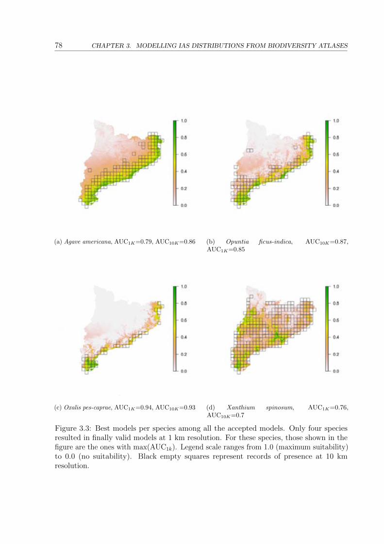
78 CHAPTER 3. MODELLING IAS DISTRIBUTIONS FROM BIODIVERSITY ATLASES
(a) Agave americana, AUC1K=0.79, AUC10K=0.86 (b) Opuntia ficus-indica, AUC10K=0.87,AUC1K=0.85
(c) Oxalis pes-caprae, AUC1K=0.94, AUC10K=0.93 (d) Xanthium spinosum, AUC1K=0.76,AUC10K=0.7
Figure 3.3: Best models per species among all the accepted models. Only four speciesresulted in �nally valid models at 1 km resolution. For these species, those shown in the�gure are the ones with max(AUC1k). Legend scale ranges from 1.0 (maximum suitability)to 0.0 (no suitability). Black empty squares represent records of presence at 10 kmresolution.

3.4. RESULTS 79
vasculars1k bias treatments and for spatial autocorrelation correction with a minimum
distance of 4250 m. Its best model was the one with the bias treatment whole area.
Opuntia ficus-indica performed well under whole area and vasculars1k bias treatments
and under both environmental and spatial occurrence �ltering, its best model being the
one with the whole area bias treatment and a spatial autocorrelation correction with
a minimum distance of 2830 m. Oxalis pes-caprae performed well under all three bias
treatments and under both spatial and environmental autocorrelation correction. Its best
model required no bias or autocorrelation treatment at all. Finally, for Xanthium spinosum
the only successful treatment was the vasculars1k bias treatment and the environmental
autocorrelation correction with a minimum distance of 0.1. Reduction in the number of
available occurrences after autocorrelation correction for the �nal four best models were:
Agave americana from 20 to 12, Opuntia ficus-indica from 13 to ten, Xanthium spinosum
from 56 to 22 and no reduction for Oxalis pes-caprae since its best model resulted in the
one without autocorrelation correction.
Table 3.4: Number of �nally accepted models per bias and autocorrelation treatment.Columns whole area, vasc1k and inv1k indicate the bias treatment scenarios for the wholestudy area, vascular plants at 1 km and IAS at 1 km, respectively. Rows correspond toautocorrelation treatments: sp 0, sp 2830 and sp 4250 correspond to minimum spatialdistances of 0 m (i.e. no treatment), 2830 m and 4250 m respectively, while env 005 andenv 01 correspond to minimum environmental distances of 0.05 and 0.1 using the Gowerdissimilarity index, respectively.
whole area vasc1k inv1k Total
sp 0 1 0 0 1sp 2830 1 2 0 3sp 4250 2 1 0 3env 005 0 0 0 0env 01 2 2 1 5Total 6 5 1 12

80 CHAPTER 3. MODELLING IAS DISTRIBUTIONS FROM BIODIVERSITY ATLASES
(a) Robinia pseudoacacia, AUC1K=0.83,AUC10K=0.52
(b) Ailanthus altissima, AUC1K=0.82,AUC10K=0.50
Figure 3.4: Examples of models that did not work. Even though these two models had ahigh AUC1K value and showed no residual autocorrelation, they had an AUC10K closeto 0.5 and are thus, not better than random. Legend scale ranges from 1.0 (maximumsuitability) to 0.0 (no suitability). Black empty squares represent records of presence at10 km resolution.
3.5 Discussion
Our results show that species distribution maps derived from presence-only records
held in biodiversity databases or atlases should be used with caution. Apparently, high
scores in predictive power from species distributions can be obtained from scarce, biased
and autocorrelated presence records using modern tools such as MaxEnt. However, our
work shows that these results can be misleading when confronted with independent data at
di�erent scales. Other authors have reached similar conclusions (Wisz et al., 2008). If the
distribution of a species was well-known at two di�erent scales, these should necessarily
be coherent with one another. In order to generate reliable �ne-resolution distribution
maps, these need to be in accordance across scales (Niamir et al., 2011). For a given
species, its real distribution map at a �ne scale should match its real distribution map at
a coarser scale once upscaled. This seems not to be the case for some species, indicating
that either the modelled distributions at �ne resolution are wrong or that the known
3.5. DISCUSSION 81
distributions at the coarser scale are, in fact, incomplete. For a well-surveyed region for
vascular plants such as our study area the latter case seems unlikely. Therefore, if one
accepts this assumption, our results suggest that distribution maps at the �ner scales are
not as good as they appear to be. If used for decision-making in conservation, they may
not accomplish the objectives for which they are meant.
Of the 20 models that performed well at 1 km resolution, only 12 were coherent with
data at 10 km resolution. Species-wise, it might seem that good �ne-scale predictive maps
could be derived from the biodiversity database for seven species. However, �ne-scale
distribution maps were in accordance with their coarser scale data for only four of them
(Table 3.3). We can thus consider the �ne-resolution maps for these four species to be
su�ciently reliable for biodiversity conservation. Coarse resolution data do not often
match the requirements of conservation planning (Ara�ujo et al., 2005) but, when this data
are assumed to re ect the distribution of the species at the coarse scale, they can be used
to make a cross-scale validation of modelled �ne-scaled distribution maps, even if high
predictive scores had been obtained. The resulting maps will be much more reliable and
robust and will help decision-makers better meet their conservation goals.
Atlas data commonly su�er from bias and autocorrelation problems (Robertson et al.,
2010). Treating both hindrances is paramount to developing robust and reliable species
distribution models (Segurado et al., 2006; Merckx et al., 2011). We tried several bias and
autocorrelation correction scenarios but did not �nd any particular pattern in our results
that can help in establishing protocols for distribution modelling. The �nal outcome of the
modelling process can only be known on a case-by-case basis. In some instances, applying
minimum spatial distances between occurrence records resulted in models without residual
spatial autocorrelation while in some other cases it was the application of a minimum
environmental distance which solved the problem. Except for a single case, Oxalis-pes
caprae, we always needed to apply some sort of occurrence �ltering in order to get rid of
residual spatial autocorrelation.
The �nal message that can be taken from this study is to be always skeptical of
�ne-resolution maps obtained when modelling species distributions from scarce and biased

82 CHAPTER 3. MODELLING IAS DISTRIBUTIONS FROM BIODIVERSITY ATLASES
data, even though they score high when measuring their predictive power. Given that
current modelling techniques and computer power allow us to run many models per species
taking into account di�erent scenarios of bias and autocorrelation correction treatments,
it is always sensible to do so and check, on a case-by-case basis, which one works best.
Having a set of independent data to validate the model seems indispensable. Cross-scale
validation, when possible, is a good solution to produce reliable and robust maps which
can then be used to make better conservation decisions.
3.6 Conclusions
Casual observations at �ne resolution in biodiversity atlases or databases have the
potential to generate continuous species distribution maps through species distribution
modelling, providing powerful tools for conservation management and planning. However,
scarcity and strong biases in the data may prevent these from being possible for many
species. Although high validation scores can be obtained when modelling this kind of
data, there is the risk that the distribution maps re ect the data distribution rather than
the true species distribution. Cross-scale validation of the data with species distribution
information at a coarser scale appears as a consistent protocol to check the validity
and robustness of �ne resolution models and thus, make them much more reliable for
decision-makers in conservation.
Fine-scale resolution maps can be derived from biodiversity atlases with problems of
data scarcity, bias and autocorrelation. However, if no independent set of data is available
to further validate them, results should be taken with precaution. When good coarser
scale data is available, cross-scale validation appears as a good choice for checking the
robustness of the data. When these options are not available, new �eld surveys may be
the only option if reliable �ne-scale maps are needed.

3.7. ACKNOWLEDGEMENTS 83
3.7 Acknowledgements
We thank Jane Elith for her insightful comments on a late version of the manuscript,
which helped to improve it, Roberto Molowny for discussion on the upscaling method,
Xavier Font for providing and giving his advice on the data and Arthur Chapman and
Robert Guralnick for their early comments and encouragement to carry out this work.
This study was supported by project CONSOLIDER-MONTES (CSD2008-00040) of the
Ministerio de Ciencia e Innovacion of the Spanish government. Xavier Pons is the recipient
of an ICREA Academia Excellence in research grant 2011-2015.

Chapter 4
Handling historical information on
protected-area systems and coverage.
An information system for the Natura
2000 European context
This chapter has been published in:
Arnald Marcer, V��ctor Garcia, Agust�� Escobar, Xavier Pons
Environmental Modelling and Software, Volume 25, Issue 8, August 2010, Pages 956-964
doi:10.1016/j.envsoft.2010.03.011
85
86 CHAPTER 4. PROTECTED AREAS’ INFORMATION SYSTEM
4.1 Abstract
Protected-area coverage is an internationally-recognized surrogate indicator for mea-
suring biodiversity conservation. To measure trends in biodiversity conservation over
time, historical records on protectedarea boundaries are needed. Protected-area systems
represent a challenge in information management for public environmental organizations.
Protected areas may be subjected to changes which must follow a mandatory multiple-step
administrative process. A wealth of information is generated which needs to be stored in
a way that eases the handling process and for future reference. We present an information
system which handles both change on protected-area boundaries over time and their related
administrative processes. It also provides distributed data maintenance functionality as
well as integrated alphanumeric, �le and cartographic information handling. We discuss
the actual implementation of the system for handling Natura 2000 sites in the Catalan and
Spanish contexts. The designed system is applicable to other European Union member
states.
Keywords protected areas, protected areas coverage, Natura 2000, historical trends,
biodiversity indicators, information systems (IS), conservation databases, protected area
boundaries
4.2. INTRODUCTION 87
4.2 Introduction
Protected areas are legal instruments specially dedicated to the protection and mainte-
nance of biological diversity (IUCN, 2010). Protected-area coverage is widely used as a
surrogate indicator, proxy, for estimating trends in the protection of biodiversity (United
Nations Environment Programme, 2009; United Nations Development Programme, 2009;
United Nations Environment Programme, 2006; European Environment Agency, 2005;
Millenium Ecosystem Assessment, 2005; Chape et al., 2005). Protected area coverage is
calculated by adding the area of each protected area in a given region as de�ned by their
boundaries.
The Convention on Biological Diversity (United Nations Environmental Programmme
(UNEP), 1992) strongly recommends that signing parties establish a system of protected
areas in order to conserve biological diversity. Spatially-enabled databases are needed
to perform gap analysis and evaluate nature protection (UNEP - WCMC, 2008; Scott
et al., 1993). Such evaluations provide important insight on where new resources should
be placed (Brooks et al., 2004; Scott et al., 1993). To analyze trends in nature protection
over time historical boundary records are needed.
Nature protection frameworks at the regional, national and international levels conform
a series of overlapping cartographic boundaries and regulations which represent not only
a major challenge for decision-making but also for information management in public
environmental organizations. These organizations need tools for querying and analyzing
this intricate and geographically-tied web of legal texts. These tools not only serve the
purpose of well-organized, accessible, comprehensive, quality and up-to-date historical
repositories of information but can also assist them in dealing with long legal processes
with con icting parties.
Current technological development in information and communication technologies
(ICT) o�ers an unprecedented opportunity to greatly enhance the handling, analysis
and public dissemination of environmental information. Governmental organizations are
required and recommended by competent bodies to make public such information (The
88 CHAPTER 4. PROTECTED AREAS’ INFORMATION SYSTEM
Council of the European Communities, 2003; World Commission on Protected Areas
(IUCN), 2005). They are responsible for providing reports and accounts of statistics on
protected areas including historical information (European Environment Agency, 2007).
The European Union nature protection policy is based upon Natura 2000, a coherent
ecological network of protected areas comprising Special Areas of Conservation(SAC)
(The Council of the European Communities, 1992) and Special Protection Areas(SPA)
(The Council of the European Communities, 1979). European Union member states are
responsible for submitting to the European Union a list of Sites of Community Importance
(SCI) for approval and declaration as SAC. After this process, protected areas may also
still preserve their former protection category. Thus, Natura 2000 represents a further level
of legal complexity. In the case of Catalonia, in a single administrative process, 73 new
protected areas have been added to the already existing list of other types of protected
areas managed by the Catalan government (Generalitat de Catalunya, 2006, 2007).
Protected areas are not static legal entities over time but undergo changes in their
regulations which follow the legal and socioeconomic contexts at any given moment. These
changes may not only a�ect the existing set of regulations but also their boundaries; i.e.,
they get extended, reduced, reclassi�ed, amalgamated with neighbouring sites, renamed,
etc. (Fish et al., 2005). To be legally valid, each of these changes must undergo a
mandatory, strict and prede�ned administrative process that involves a series of steps
starting at the initial proposal by the promoting party, e.g., the public administration, and
ending with the publication of the approved legal text in the o�cial governmental bulletin.
Each of these steps may introduce interim changes in the working set of boundaries;
some of them due to claims placed by a�ected parties, i.e., local administrations and the
public in general. An accurate handling of all this information is crucial for an e�ective
guidance of the process and for ensuring adequate treatment of this external participation.
Historical digital archives, i.e., databases, represent a fundamental tool for handling all
this information. They also provide the base from which it is possible to understand the
historical context of protected area establishment (UNEP - WCMC, 2008; United Nations
Economic Commission for Europe (UNECE), 1998) and evaluating protected area coverage

4.2. INTRODUCTION 89
over time is possible.
Handling of historical information in reference protected area databases To
our knowledge, only the World Database on Protected Areas (WDPA) holds information on
historical changes in protected areas (UNEP - WCMC, 2009; Chape et al., 2005; Fish et al.,
2005). However, the scope and aim of the WDPA is quite di�erent from the information
system we present. WDPA is a global compilation of information o�ered via a web site
in a digested way. As of February 2010, Natura 2000 sites are still not available at the
WDPA (IUCN-UNEP, 2010; UNEP - WCMC, 2009). We present an information system
which handles historical versions of protected area boundaries and assists in handling the
administrative work involved in protected area declaration, modi�cation and termination.
The Protected Areas Database of the United States of America is a collaborative
e�ort between governmental and non-pro�t organizations. Its latest downloadable version,
released April 2009, does not contain historical information and its plans only include
the date of establishment of protected areas for a later date(GreenInfo Network, 2008;
Conservation Biology Institute, 2008).
In Australia, the Collaborative Australian Protected Areas Database (CAPAD) is a
textual and spatial database compiled from information supplied by the Australian, State,
and Territory Governments and other protected area managers (Australian Department
of the Environment, Water, Heritage and the Arts, 2008). CAPAD's GIS layer contains
only the latest valid boundaries with only information on the gazettal date of the original
proclamation and the date of the most recent gazetted amendment but not a complete
historical record of changes (Australian Department of the Environment, Water, Heritage
and the Arts, 2008; Australian Department of the Environment and Heritage, 2004).
The European Common Database on Designated Areas (CDDA) o�ers information
on the nationally designated sites for the Natura 2000 ecological network (European
Environment Agency, 2009b). The CDDA database holds only information on the gazettal
date of original declaration and latest amendment but not its historical track (European
Environment Agency, 2009c). There is a recommendation that the structure be redesigned
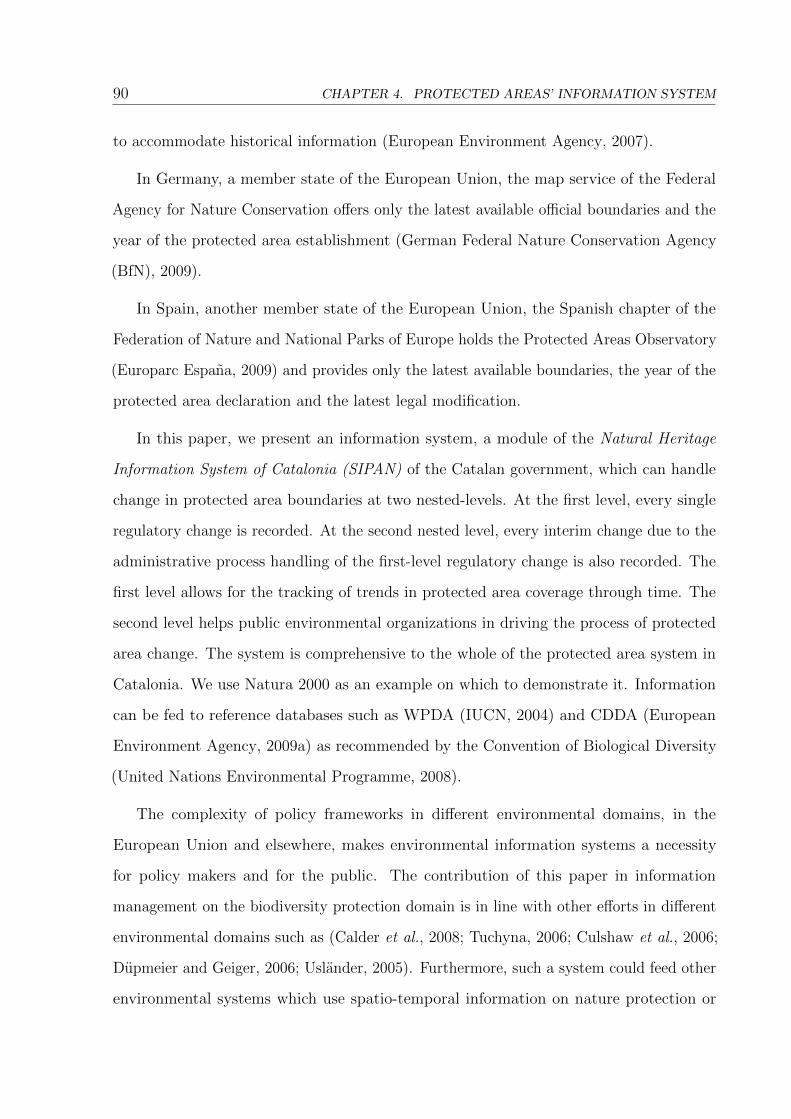
90 CHAPTER 4. PROTECTED AREAS’ INFORMATION SYSTEM
to accommodate historical information (European Environment Agency, 2007).
In Germany, a member state of the European Union, the map service of the Federal
Agency for Nature Conservation o�ers only the latest available o�cial boundaries and the
year of the protected area establishment (German Federal Nature Conservation Agency
(BfN), 2009).
In Spain, another member state of the European Union, the Spanish chapter of the
Federation of Nature and National Parks of Europe holds the Protected Areas Observatory
(Europarc Espa~na, 2009) and provides only the latest available boundaries, the year of the
protected area declaration and the latest legal modi�cation.
In this paper, we present an information system, a module of the Natural Heritage
Information System of Catalonia (SIPAN) of the Catalan government, which can handle
change in protected area boundaries at two nested-levels. At the �rst level, every single
regulatory change is recorded. At the second nested level, every interim change due to the
administrative process handling of the �rst-level regulatory change is also recorded. The
�rst level allows for the tracking of trends in protected area coverage through time. The
second level helps public environmental organizations in driving the process of protected
area change. The system is comprehensive to the whole of the protected area system in
Catalonia. We use Natura 2000 as an example on which to demonstrate it. Information
can be fed to reference databases such as WPDA (IUCN, 2004) and CDDA (European
Environment Agency, 2009a) as recommended by the Convention of Biological Diversity
(United Nations Environmental Programme, 2008).
The complexity of policy frameworks in di�erent environmental domains, in the
European Union and elsewhere, makes environmental information systems a necessity
for policy makers and for the public. The contribution of this paper in information
management on the biodiversity protection domain is in line with other e�orts in di�erent
environmental domains such as (Calder et al., 2008; Tuchyna, 2006; Culshaw et al., 2006;
D•upmeier and Geiger, 2006; Usl•ander, 2005). Furthermore, such a system could feed other
environmental systems which use spatio-temporal information on nature protection or

4.3. LEGAL CONTEXT 91
land-use for a range of environmental analyses including global change (Schaldach and
Alcamo, 2006).
4.3 Legal context
The Birds and Habitats directives constitute the basic European policy framework
for nature conservation (The Council of the European Communities, 1992, 1979, 1997).
They declare Natura 2000 as a coherent ecological network composed of Special Areas of
Conservation (SAC). SAC represent sites in need of conservation for containing habitats of
European value or parts of the distribution areas of species of European value. In the case
of Spain, several legal texts transpose these directives and establish the legal framework
by which regional governments, e.g. the government of Catalonia, are entitled to propose
and declare Natura 2000 sites (Gobierno del Estado Espa~nol, 1998, 1995, 1989).
The government of Catalonia, coordinated with the rest of regional governments by
the Spanish Government, submitted to the European Union the list of Sites of Community
Importance (Generalitat de Catalunya, 2006, 2007; Parlament de Catalunya, 2006). All
sites proposed as SCI are incorporated into the Catalan protected area network.
The administrative process, from proposal to official approval
The handling of an Administrative process, such as that of declaration of SACs, involves
a set of prede�ned steps by which an initial government proposal ends in the �nal approval
of some sort of action, e.g., the declaration of a new protected area.
The approval of Natura 2000 Special Areas of Conservation is a three-step process
(European Commission, 1997): �rst, member states make a draft proposal of a list of Sites
of Community Importance. Second, the European Commission in agreement with the
member states, establishes the list as o�cial. Third, member states designate the sites
as Special Areas of Conservation providing them with protected area status. Figure 4.1
illustrates this process for Catalonia.
Our system solves the challenge of handling all information involved in administrative
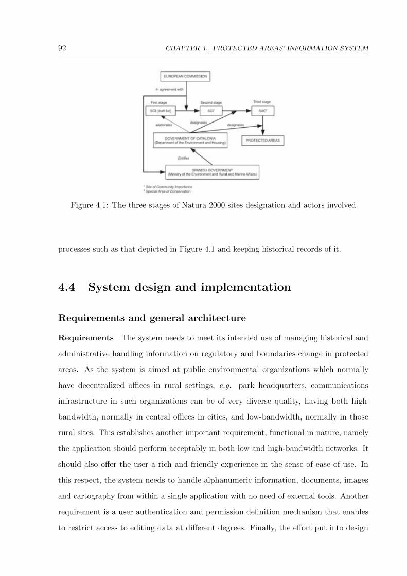
92 CHAPTER 4. PROTECTED AREAS’ INFORMATION SYSTEM
Figure 4.1: The three stages of Natura 2000 sites designation and actors involved
processes such as that depicted in Figure 4.1 and keeping historical records of it.
4.4 System design and implementation
Requirements and general architecture
Requirements The system needs to meet its intended use of managing historical and
administrative handling information on regulatory and boundaries change in protected
areas. As the system is aimed at public environmental organizations which normally
have decentralized o�ces in rural settings, e.g. park headquarters, communications
infrastructure in such organizations can be of very diverse quality, having both high-
bandwidth, normally in central o�ces in cities, and low-bandwidth, normally in those
rural sites. This establishes another important requirement, functional in nature, namely
the application should perform acceptably in both low and high-bandwidth networks. It
should also o�er the user a rich and friendly experience in the sense of ease of use. In
this respect, the system needs to handle alphanumeric information, documents, images
and cartography from within a single application with no need of external tools. Another
requirement is a user authentication and permission de�nition mechanism that enables
to restrict access to editing data at di�erent degrees. Finally, the e�ort put into design

4.4. SYSTEM DESIGN AND IMPLEMENTATION 93
and development of such an application should also be of use when developing the version
o�ered for public dissemination of information.
General architecture The system is structured in three layers as shown in Figure
4.2. The �rst layer is a rich-client desktop application which handles queries and results,
builds the business-logic objects and interacts with the user. The second layer is a server
application which translates requests sent by the client in the form of Java objects into
SQL (Structured Query Language) queries understandable by the database, converts the
result sets from the database to data arrays stored in a single instance of a Java object,
compresses the object in order to speed data transfer, and sends it back to the client.
The third layer is a data persistance unit consisting of a back-end relational database
management system.
Caching and editing functionality Data retrieved from the database are locally
stored, cached, in the user's directory, enabling the desktop application to work with
local data instead of having to go back and forth from the database. When needed,
these cached data are synchronized with the database back-end: at user request or when
entering editing mode. The user can always request the latest available information for
that particular protected area by synchronizing the local cache with the database. This
caching mechanism ensures higher responsiveness of the application and a richer user
experience both in high and low-bandwidth contexts.
The application is meant to share data editing tasks in a distributed way. In order to
prevent collisions in data editing between di�erent users, a record-blocking mechanism
enabled at the protected area level ensures that at any given moment only one user is able
to modify data on a given protected area. Once the user is done with the modi�cations on
the protected area the block is released and the area is available again for further editing.
Document and image handling The application allows to attach as many documents,
e.g. legal texts, and images to a protected area as needed. Speci�c panels allow the
handling of this type of information. Documents and images are sent by the client as
binary streams and stored as binary large objects in the database back-end. For size and

94 CHAPTER 4. PROTECTED AREAS’ INFORMATION SYSTEM
Figure 4.2: General architecture of the system. A server application mediates betweenthe client and the database. It sends data in a compressed form to the client, whichuncompresses them and keeps a local cache synchronized with the database. Data(alphanumeric, documents, images and cartography) are stored in a central databaserepository.
performance reasons, documents and images are not cached. They are retrieved from the
database on demand and not locally stored. Documents can be attached at the level of the
protected area and at the level of administrative step. This enables each administrative
step to hold its resulting legal text.
Cartography We developed a cartography browser/editor tool which is embedded at
di�erent places within the application, i.e. at the protected area level for visualizing
the latest valid boundaries and at the administrative process step. In the latter case,
it stores each version corresponding to each interim change in boundaries. The version
held at the last administrative step of the latest approved legal text contains the current
valid boundaries for the protected area. The tool relies upon existing OGC-compliant
WMS servers for o�ering background cartographic layers onto which boundaries can
be displayed and edited. The usual visualizing (pan, zoom) and editing (points, lines,
polygons) capabilities are o�ered. Also, boundaries can be imported from text �les in
MiraMon (Pons, 2004) format. In memory, boundaries are stored as objects conformant
to Open Geospatial Consortium Standards (Open Geospatial Consortium Inc, 2006). In
the database back-end they are persisted as relational data. For the same reason as with
documents and images, boundaries are not included in the local cached data but are
retrieved when needed. Since most times the user will only work with the latest valid
boundaries of a protected area, for performance reasons a redundant copy of the last valid

4.4. SYSTEM DESIGN AND IMPLEMENTATION 95
limits is stored in a compressed zip �le in the database. However, contrary to what was
done with documents and images, once at the client they are stored in the local �le system
temporarily. This makes the process of retrieving such cartographic information from the
database much faster.
Object model
Classes and interfaces The major classes of objects in our design can be seen in Figure
4.3. The Protected area class is the key target of our system; it holds all information
associated with protected areas in a tree-like structure. Each protected area object contains
the administrative process objects that a�ect it and, in turn, each administrative process
object contains the set of administrative step objects that conform its mandatory handling.
The �nal administrative step object ends with the publication of the Legal text in the
government's o�cial journal which declares, modi�es or terminates its parent protected area
object. Each step may also reference a Geometry object which represents the boundaries
set at that particular step. This results in an e�ective storage of all versions of the
boundaries along the process. The �nal approved boundaries by the Legal text are held by
the last step.
An administrative process is comprised of a speci�c set of mandatory Handling steps.
At some point, i.e. handling step, public and local administrations are allowed and
encouraged to participate. This participation may end in a list of claims to the proposal
being considered. Some of these claims may be positively considered and end up in
modi�cations of the Legal text and/or Geometry.
Since an administrative process may a�ect one or more protected areas, the list of
administrative process objects is not directly contained within the list of protected area
objects. Instead, each protected area object has a list of references that point to the
administrative process objects that a�ect it. On the other hand, each administrative step
belongs only to one administrative process, and thus, the object is contained within this
administrative process. An administrative process may a�ect a given protected area in
more than one way, e.g. it may rename it, rede�ne its boundaries, etc. The responsibility
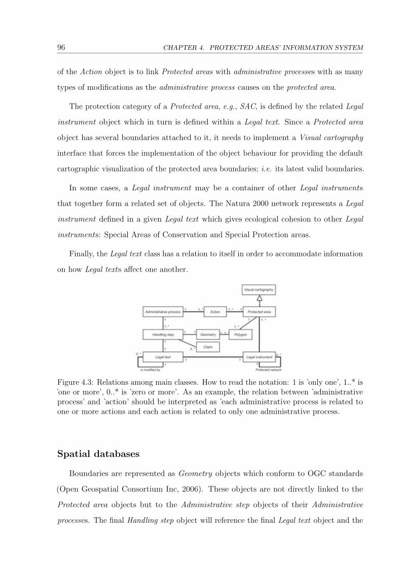
96 CHAPTER 4. PROTECTED AREAS’ INFORMATION SYSTEM
of the Action object is to link Protected areas with administrative processes with as many
types of modi�cations as the administrative process causes on the protected area.
The protection category of a Protected area, e.g., SAC, is de�ned by the related Legal
instrument object which in turn is de�ned within a Legal text. Since a Protected area
object has several boundaries attached to it, it needs to implement a Visual cartography
interface that forces the implementation of the object behaviour for providing the default
cartographic visualization of the protected area boundaries; i.e. its latest valid boundaries.
In some cases, a Legal instrument may be a container of other Legal instruments
that together form a related set of objects. The Natura 2000 network represents a Legal
instrument de�ned in a given Legal text which gives ecological cohesion to other Legal
instruments: Special Areas of Conservation and Special Protection areas.
Finally, the Legal text class has a relation to itself in order to accommodate information
on how Legal texts a�ect one another.
Figure 4.3: Relations among main classes. How to read the notation: 1 is `only one', 1..* is`one or more', 0..* is `zero or more'. As an example, the relation between `administrativeprocess' and `action' should be interpreted as `each administrative process is related toone or more actions and each action is related to only one administrative process.
Spatial databases
Boundaries are represented as Geometry objects which conform to OGC standards
(Open Geospatial Consortium Inc, 2006). These objects are not directly linked to the
Protected area objects but to the Administrative step objects of their Administrative
processes. The �nal Handling step object will reference the �nal Legal text object and the

4.4. SYSTEM DESIGN AND IMPLEMENTATION 97
Geometry object corresponding to the boundaries set by it. Therefore, a given Protected
area object has access to all Geometry objects, i.e. boundaries, that form their historical
coverage evolution. Thus, Protected area objects can be queried for all their chronologically
ordered changes that, through Legal texts, have led them from their declaration to the
latest valid boundaries (see `F' and `G' in Figure 4.4). Historical changes can thus be
traced and coverage change through time evaluated for the whole network.
Geometry objects can be accessed from the Legal text objects that de�ne them. Since
a given Legal text may declare, modify or terminate any number of protected areas, it
is necessary to label all polygons contained in their referenced Geometry objects with
the Protected area object they belong to (Figure 4.3). This can be done with a speci�c
tool in the cartography panel of the application (see `D' in Figure 4.4). With this design,
boundaries can be retrieved both from the Administrative processes that led to them and
from the protected areas they a�ect but only one single copy of each boundary is handled
and stored by the system.
Technology used
We developed the whole system around Java technology1, and used Oracle 9i2 as
the database back-end. The application has been targeted to the Java 1.5+ versions.
Background cartography is collected from available WMS-compliant servers. We also make
use of the open source libraries Java Topology Suite3 and JasperReports4. The system is
designed in such a way that it can also work with other databases such as MySQL5.
Deployment
The application is deployed via Java Web Start Technology6 which allows for authomatic
updating of client applications. This proves a convenient way to ensure that users always
have the latest available version.
1http://java.sun.com2http://www.oracle.com/index.html3http://www.vividsolutions.com/jts/jtshome.htm4http://www.vividsolutions.com/jts/jtshome.htm5http://www.mysql.com/6http://java.sun.com/javase/technologies/desktop/javawebstart/index.jsp
98 CHAPTER 4. PROTECTED AREAS’ INFORMATION SYSTEM
User interface
The client layer is an application with querying, visualizing, editing and exporting
capabilities.
User authentication and permissions To enter the system the user needs to authen-
ticate through a login panel using a user name and a password. Once authenticated, data
are loaded from the database if not already cached. Editing permission can be given
on a per-protected-area basis. This allows for distributed curatorship of protected area
information. Each protected area management team can take care of the information of
their own protected area. By default, all users have read-only access to all information.
Data entry Data are entered by means of several entry forms (see `A, B, C, D' in
Figure 4.4): one for basic protected area information, another for administrative processes
and others for thesaurus-like information, e.g., legal texts. With the protected area form,
the user enters basic information such as code, name, and protection category. In the
administrative process form, the user enters data on all administrative processes and
their handling steps. Documents and cartography can be entered within each step. Since
cartography representing the boundaries of the protected areas is de�ned in the legal
texts, both are entered at the same level in this data entry form. The last step of an
administrative process contains the cartography �nally approved by the process and each
previous step may contain drafts of the cartography that led to this �nal version. Once
the cartography, i.e., the polygonal boundaries, has been entered, each polygon is linked
to the corresponding protected area object it applies to. Thus, only a single copy of
the boundaries exist and is accessible both from the protected area object and from
the administrative process and legal text objects. From within the protected area form,
administrative processes with their associated legal texts and cartography are visible (see
`D' in 4.4), but not editable.
Query and visualization The application o�ers multiple-criteria �ltering functionality
through a speci�c panel. Once data are �ltered, all data entry, query and visualizing panels
can be set to only show the �ltered subset of elements. A tree-like display of protected

4.4. SYSTEM DESIGN AND IMPLEMENTATION 99
Figure 4.4: Partial screenshots of the user interface for entering (as explained in Figure4.5) and querying protected area data. Once data are entered all legal texts a�ectingeach protected area become visible. A time slider control (please note it in `G') in thecartography browser allows the visualization of historical cartographic boundaries
areas and administrative processes o�ers the user data browsing, editing and reporting
capabilities from within it. A navigator panel allows the user to step through all protected
areas and administrative processes and to directly go to a given one selected from a list.
Sites can also be browsed through a hierarchical tree navigator. Protected area boundaries
can be visualized individually in the protected area panel or together (using the �lter or
not) in a general cartography panel.

100 CHAPTER 4. PROTECTED AREAS’ INFORMATION SYSTEM
Reports, graphics and data export Several reporting templates are available for
producing reports of single objects (protected areas or administrative processes) and
multiple objects in an aggregated form; e.g. protected area coverage per category type and
administrative unit. Several types of graphics can be dynamically obtained by choosing
prede�ned sets of dependent and independent variables. The user can customize exports
of data to CSV (Comma Separated Values). Cartographic data can also be exported to
the MiraMon GIS format. When producing reports, graphics or exports the user may
choose whether to use the full or the �ltered dataset.
Functionality example
In this subsection, we give an overview on how to manage the process of declaration of
a new protected area with its set of boundaries and the process of adding a new set of
boundaries to an existing protected area. Figures 4.4 and 4.5 illustrate this.
Protected area declaration The necessary actions a user must take care of when
addressing the process of declaration of a new protected area can be seen in Figure 4.5.
In the case of Natura 2000 sites, the process starts by creating a new protected area
of protection type Natura 2000. Once created, the application adds it to the system's
protected area list. The second step involves adding a new administrative process to the
administrative process list ; that is, a container for the information regarding the handling
of protected area declaration information. Then, we associate it to the protected area
created before and assign a declaration action type to it. This is done by selecting the
protected area from the corresponding dropdown lists in the administrative process data
entry panel. Thus, we now have an open administrative process for handling the process
of declaration of a new Natura 2000 site. Through the real administrative process, every
single handling step taken will be added to this declaration process. In Figure 4.1, we
can see the three main stages, i.e. handling steps, which involve the declaration of a
Natura 2000 site. There may also exist other intermediate steps in between the three
main stages seen in Figure 4.1. The list of prede�ned mandatory handling steps for each
type of administrative process is entered into the system. Then, the user �lls each of
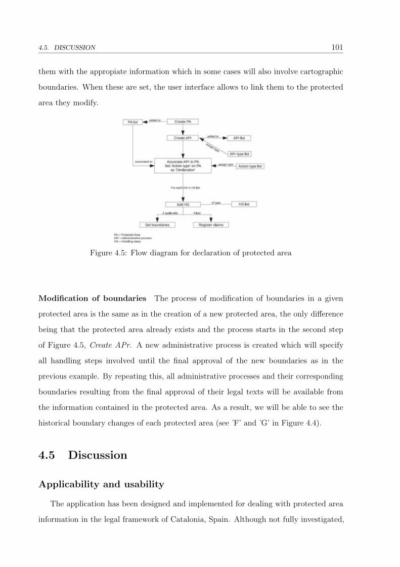
4.5. DISCUSSION 101
them with the appropiate information which in some cases will also involve cartographic
boundaries. When these are set, the user interface allows to link them to the protected
area they modify.
Figure 4.5: Flow diagram for declaration of protected area
Modification of boundaries The process of modi�cation of boundaries in a given
protected area is the same as in the creation of a new protected area, the only di�erence
being that the protected area already exists and the process starts in the second step
of Figure 4.5, Create APr. A new administrative process is created which will specify
all handling steps involved until the �nal approval of the new boundaries as in the
previous example. By repeating this, all administrative processes and their corresponding
boundaries resulting from the �nal approval of their legal texts will be available from
the information contained in the protected area. As a result, we will be able to see the
historical boundary changes of each protected area (see `F' and `G' in Figure 4.4).
4.5 Discussion
Applicability and usability
The application has been designed and implemented for dealing with protected area
information in the legal framework of Catalonia, Spain. Although not fully investigated,
102 CHAPTER 4. PROTECTED AREAS’ INFORMATION SYSTEM
the same design should apply seamlessly to the rest of regional governments in Spain since
all depend on the same Spanish and European legal frameworks. For the very same reason,
this design should also be applicable to other member states of the European Union with
minimal tuning of the application and database. The application has been implemented
with multiple-language support.
The application has been tested by entering data (alphanumeric, documents, images
and boundaries) corresponding to over 450 protected areas of di�erent protection categories
and to more than 130 administrative processes which declare, modify or terminate these
protected areas. The system has proved useful for handling and storing such diverse set
of cases, protected areas of di�erent category linked through di�erent action types to
di�erent types of administrative processes and legal texts.
One of the main bene�ts in ease of use for the �nal user is the integration of tools
for dealing with di�erent kinds of information (alphanumeric, �les and cartography) on
a single application. The user does not need to leave the application when handling the
cartographic representation of the protected areas, e.g. boundaries.
Performance issues
Environmental public administrations may have buildings located in areas with low-
bandwidth connections. Being able to browse and edit protected area information including
documents, images and cartography located in remote servers is a di�cult task. Developing
applications that deal with large volumes of data and that respond readily to user interac-
tion represents sometimes an unattainable goal without improving network infrastructures.
We have experienced that traditional web applications have proved unsatisfactory in
performance terms in low-bandwidth contexts since many client-server interactions are
needed and, as a result, application performance is severely degraded, leaving the user with
frozen and unresponsive screens. AJAX7 technologies provide performance improvements
though user interfaces are not as powerful as rich-client desktop applications. Rich-client
technologies also present performance issues if no caching mechanism is used. Resultset
7Asynchronous Javascript and XML
4.5. DISCUSSION 103
cursors from database queries slow down the application when accessed from remote clients.
The caching mechanism we developed minimizes client-server interaction and improves
application performance and responsiveness. Clients only have an initial delay when
loading data for the �rst time. Then, the application works with a local cache of this data
and synchronizes it with the database back-end when needed. Since the application has all
data either in-memory or on-disk, performance and responsiveness are greatly enhanced.
A disadvantage of this technique over web applications is that clients need to have a Java
virtual machine pre-installed, although this is partially solved as most users normally
already have it. Although web applications do not present this disadvantage, the existence
of unavoidable di�erences in behaviour of di�erent Internet browsers are also a factor that
substantially increases the development e�ort when developing web applications. However,
more development e�ort is being put into further decoupling the presentation layer and
the business layer so that it becomes possible to o�er both a web and desktop interface
working against the same business layer. A web presentation layer could be o�ered for
public consultation and a richer desktop application would be used for intensive work by
the technical sta� of the public administration.
Error control
Two types of errors can a�ect the system. The �rst type of errors originates from
the process of data entry itself; i.e. errors can be committed to the database when a
user enters data. To minimize such errors, data entry form controls use �eld validation
and lookup tables. However, expert revision of data before making it public is necessary.
Boundaries are �rst �nely digitized with a GIS software package using quality reference
cartography, mainly 1:5000 topographic maps, and then imported into the system. The
second type of errors are those derived from using di�erent cartographic datasets in di�erent
moments. Historical boundaries are de�ned using their contemporary reference cartography.
Reference cartography such as topographic maps and orthophotos is in a constant process
of revision and improvement. As reference cartography changes, protected area boundaries
must also change in order to be perfectly �tted to current o�cial cartography. This second
104 CHAPTER 4. PROTECTED AREAS’ INFORMATION SYSTEM
type of error has a much more di�cult solution. One can only try to estimate it and take
it into account when comparing protected area coverage between two datasets that used
di�erent reference cartography. Although it is beyond the scope of this paper and not
explored, we think this error may not represent important changes in overall protected area
coverage estimation. Calculated coverages and trends should di�er minimally. Another,
more costly and almost impractical solution would be to always manually update protected
area boundaries to the most recent reference cartography. However, a drawback would be
that a protected area represented on top of the reference cartography used for digitizing it
would not �t correctly and would work against other uses such as visual representation of
historical cartography.
Benefits of the system
Having structured historical information on protected area boundaries for all protection
categories in a given territorial extent provides several bene�ts. First, it allows to monitor
protected area coverage over time, i.e. a surrogate indicator of biodiversity protection.
Second, having organized and spatially-explicit historical information on protected areas
raises the possibility of performing cross-analyses with many other datasets on population,
agriculture, forestry, local planning, etc. Such analyses may allow to discover the social,
economical and political factors driving changes in protected area coverage over time
and predict future land protection scenarios. Third, such systems can become important
data providers for international e�orts at data gathering for analysing global trends in
protected area coverage such as WDPA. In addition, they can be converted into web
services, similar to other web services in di�erent environmental domains (Goodall et al.,
2008; Tuchyna, 2006), which can deliver on-demand protected area boundaries for a given
historical moment. Our system represents a superset of information held by WDPA for its
minimum and core set of attributes (UNEP - WCMC, 2010). Feeding data into WDPA
can be done by exporting information as speci�ed in WDPA Data Standards. Work is in
progress for also covering its enhanced set of attributes. Currently, there exist licensing
and/or publishing restrictions on submitting data to WDPA on Natura 2000 sites (UNEP

4.6. CONCLUSIONS 105
- WCMC, 2009), although UNEP-WCMC is working to solve them. And �nally, such type
of systems become almost mandatory for public environmental organizations in order to
make a proper custody of such information while providing advanced information services
to individual citizens, the private and the public sector.
Further work
Further work will be aimed at enriching the database with information on habitats and
species present in the protected areas and on planning and management information. With
respect to the application, we will concentrate our e�ort on improving the user experience
by further improving the application performance, i.e., making the local cache mechanism
more e�cient, and expanding the application features such as adding more custom-made
maps, reports and graphics. We are currently working on enabling the application to
import and export cartography in the OGC-standard GML format8.
Developments are currently under way to further separate the presentation and business
layers so that the client layer can be o�ered both as a rich desktop client application or
as a thin web application working against the same business logic layer. The former is
aimed at the government's administrative and technical sta� and the latter at bringing
information to the general public without the need to fully develop a separate environment.
Currently, cartographic data are stored and o�ered to the user in the UTM-ED50
reference system. We plan to convert these data from the current ED50 datum to the
new pan-European ETRS89 datum, as recommended by resolution of the European IAG
Reference Frame Sub-Commission for Europe (International Association of Geodesy, 1990)
and mandated by the Spanish regulation (Gobierno del Estado Espa~nol, 2007).
4.6 Conclusions
We have presented an information system for helping public administrations in dealing
with the complex and interwoven set of information regarding protected areas, adminis-
trative processes and legal texts. For any type of legally de�ned protection category, it
8Geography Markup Language

106 CHAPTER 4. PROTECTED AREAS’ INFORMATION SYSTEM
can handle historical information, including boundaries, on the administrative processes
involved in protected area declaration, modi�cation and termination. Thus, it can monitor
protected area coverage over time, a surrogate indicator of biodiversity protection.
Regional and national governments can also bene�t from such a system for feeding data
to reference databases such as the World Database on Protected Areas and the European
Common Database on Designated Areas.
4.7 Acknowledgements
The work reported here has been possible thanks to support from the General Direc-
torate of the Natural Environment of the Department of the Environment and Housing of
the Autonomous Government of Catalonia. Also, the authors wish to thank the anonymous
reviewers for greatly helping in improving the original paper.

Chapter 5
General discussion, conclusions
and further research
5.1 General discussion
This dissertation has two main focus points: a) how to stretch the possibilities of scarce,
problematic species occurrence data to derive information which is useful in conservation
planning and management (Chapters 2 and 3) and b) how to organise information on
biodiversity protection, i.e. protected areas' boundaries, to be combined with the former
in biodiversity conservation assessments (Chapter 4). It combines concepts and tools
from three very broad �elds: biodiversity conservation, species distribution modelling and
information systems. Such interdisciplinary research is important in order to face the
biodiversity conservation challenges society has (Krishtalka and Humphrey, 2000; Schnase
et al., 2003). We live in a rapidly changing world which threatens many of the given assets
that nature provides us (Sala et al., 2000). One of these assets is biodiversity, at all of its
levels, from genes up to whole biomes and the Biosphere. Biodiversity is essential to our
survival and well-being (Pimm et al., 1995). It is thus of paramount importance to make
the best use of the available tools we have: a large growing amount of data compiled in
biodiversity databases and new sophisticated modelling tools which can help in dealing
with several shortcomings of those data.
107

108 CHAPTER 5. GENERAL DISCUSSION AND CONCLUSIONS
Biodiversity data, however problematic, is a fundamental asset at our disposal to tackle
the problem of biodiversity conservation. Within the scope of this dissertation and in order
to explore new avenues and ways of making the best use of available species' occurrence
data I have chosen two conservation challenges as examples to work with. In Chapter 2, I
have examined how to use available species occurrence data to model SCI to assess their
conservation and protection status. In Chapter 3 we explored the other side of the coin:
to what degree can we pull occurrence data held in biodiversity databases to assess the
threat posed to native biodiversity by IAS. In the �rst case, the knowledge gained can
lead to the identi�cation of priority areas for conservation as in Cabeza et al. (2004) and,
in the second case, of areas with risk of invasion by alien species as in Jim�enez-Valverde
et al. (2011). If protected areas are our biodiversity crown jewels we need to assess their
e�ectiveness in protecting native biodiversity and the extent to which they are under
threat.
An important and often overlooked aspect of data is that of organisation and availability.
Protected areas are a very cost-e�ective means (Balmford et al., 2002) and a cornerstone
in biodiversity protection (Margules and Pressey, 2000; Rodrigues et al., 2004b). We
have chosen protected areas' boundaries as an example case of the issues involved in data
organisation and availability. Protected areas boundaries are quite a complex problem of
data organization as we have seen in Chapter 4. Tackling this kind of problem allowed us
to link primary biodiversity data exploration and modelling with biodiversity conservation.
The aim of this �nal chapter is to discuss and highlight, from a broad perspective,
the knowledge gained during the development of the work that led to this dissertation,
particularly as regards to the use of these methodologies and technologies for biodiversity
conservation. First, I will focus on the particularities of primary biodiversity data and
environmental data, their availability and usability. Second, I present my general con-
clusions about species modelling tools for range map generation. Finally, I provide an
overview of the issues that need to be addressed with when organising data on protected
areas boundaries.
5.1. GENERAL DISCUSSION 109
The need for data
Occurrence data
The quality of species occurrence data in all of their facets (see Figure 1.1 in Chapter 1),
specially bias and autocorrelation, together with data quantity, greatly determines how to
approach distribution modelling. Despite using the same algorithm, Maxent (Phillips et al.,
2006), di�erent approaches were needed due to the di�erences of data quality between the
SCI dataset used in Chapter 2 (high-quality data with relatively lower bias) and the IAS
dataset used in Chapter 3 (data of unknown quality with strong bias). Maxent has been
used for both SCI and IAS due to the favorable reviews of the algorithm for modelling
presence-only data with a limited number of occurrences (Elith et al., 2006; Hernandez
et al., 2006; Phillips and Dud��k, 2008; Wisz et al., 2008; Elith and Graham, 2009; Thorn
et al., 2009; Costa et al., 2010) and even with bias present (Phillips et al., 2009; Rebelo
and Jones, 2010).
While data used in the modelling of SCI, although scarce, were of high quality, data
used in the modelling of IAS had problems typical of ad-hoc occurrence data compiled in
digital atlas databases (Robertson et al., 2010). In the �rst case, since they are rare species
of high conservation and scienti�c interest, their degree of prospection is much higher than
that with other more common species, specially so in an already well-prospected study
area, as in (Marmion et al., 2009). Thus, it is more likely that the geographic range of
the species is better re ected by rare species occurrences than with other more common
species. These kind of data were the subject of study in Chapter 2. Also in this case, they
were compiled and checked record-by-record and it could be safely assumed that all unique
occurrence records are correctly identi�ed and georeferenced. Another quality of these data
is that they span over the whole realised range of the species; the probability of discovering
new populations beyond their current known Extent of Occurrence (EOO) is quite low
(Lloren�c S�aez, personal communication). Altogether, the level of con�dence in the quality
of these data is of a much higher degree than with the IAS dataset used in Chapter 3.
In this latter case, data were obtained from a digital database encompassing all groups

110 CHAPTER 5. GENERAL DISCUSSION AND CONCLUSIONS
of organisms and species. This database was compiled with semi-automatic digitisation
methods and, although quality checks have been made, they are not comparable to a
species-by-species and record-by-record check in the case of the SCI dataset.
Spatial autocorrelation among occurrence records is another important aspect regarding
data quality in species distribution modelling (Dormann et al., 2007). Spatial autocorrela-
tion may help in ate measures of accuracy for presence-only distribution models (Veloz,
2009) and, as a consequence, model performance may be overestimated. In order to
account for autocorrelation, a set of preventive treatments were done to both datasets, SCI
and IAS. Instead of a single model per species, multiple models were run from multiple
datasets per species; each one containing a di�erent �ltered subset of species occurrence
records (in each one, occurrence records were guaranteed to be at least at a given euclidean
or environmental euclidean distance from each other). This methodology proved e�ective
in removing residual spatial autocorrelation. Of all the models run per species, those with
residual spatial autocorrelation were discarded.
Another important aspect of data quality is that of bias or uneven sampling of the
geographical and environmental spaces (Phillips et al., 2009). Bias was treated di�erently
for the SCI and IAS datasets. In the SCI dataset case, bias was assumed to be low and
thus, of little or no impact on the �nal models. On the other hand, in the IAS dataset
case, bias was known to be high and the target-group background strategy de�ned by
Phillips et al. (2009) was applied.
These data particularities determined the modelling strategy taken in Chapters 2 and
3. Knowledge of the quality of the data greatly determines the modelling strategy, as
has been shown for both SCI and IAS cases. In Chapter 2, the con�dence on the high
quality of the occurrence data allowed for safely assuming the resulting models as fairly
acceptable and thus, ready for conservation assessment. However, in the case of IAS, in
Chapter 3, two situations concurred: problematic �ne-resolution data combined with their
coarser-resolution counterpart which was assumed to approximate the species distribution
at this coarser resolution. This lead us to use this coarser dataset as a second check for
model perfomance. A novel cross-scale validation technique was devised to further check

5.1. GENERAL DISCUSSION 111
the validity of the models against these much coarser resolution data. The study area,
Catalonia, is reasonably well prospected for vascular plants at coarse resolutions such
as 10-by-10 km (Pino et al., 2005) and, occurrences can be assumed to re ect the true
distribution of the species at this resolution. Therefore, we can argue that, once upscaled,
�ner resolution models should be in accordance with these data at a coarser scale in order
to be considered as acceptable. This cross-scale validation con�rmed our suspicion on
the con�dence of the performance measures of �ne-resolution models. It resulted in the
acknowledgement that, even if apparently valid, �ne-resolution models had to be taken
with caution since for some species they did not agree with their coarser data.
An obvious general prerequisite is that good quality data is always necessary when
modelling species distributions (Robertson et al., 2010). As has been proved, in the case
of poor or unknown-quality data, it is convenient to have a target benchmark with which
to compare them. However, when good quality data is at hand, we can be more con�dent
in the resulting models and accept them as our best approximations to species ranges.
Assumptions are inherent to species distribution modelling and, to some degree, they need
to be formulated and accepted (Wiens et al., 2009).
While biodiversity databases need to be improved in quantity and quality (Hortal
et al., 2007), in the meantime we need to deal with unknown uncertainty. Most primary
biodiversity data present problems of scarcity and quality (Robertson et al., 2010) but
this should not lead to inaction (Wiens et al., 2009). When uncertainty is known it can be
treated formally and results be given with con�dence valuations. When it is unknown we
can only try to be as rigorous as possible and make the best educated guesses possible at
the time of modelling and analysing results. Failing to do so would render all this wealth
of information useless. It is better to have information on a species distribution based on
an educated guess rather than not having any information at all. Not using models is not
an option and managers must be satis�ed with a level of certainty that is good enough to
move forward (Wiens et al., 2009). Conservation cannot a�ord waiting for perfect data to
be available. Sensible use of the data and modelling techniques can give value to existing
biodiversity data in providing good information tools for conservation; as in Bustamante

112 CHAPTER 5. GENERAL DISCUSSION AND CONCLUSIONS
and Seoane (2004).
Environmental data
Spatially exhaustive environmental data are the second source of input data for species
distribution models (Peterson et al., 2011). Their relevance for the species ecological
requirements and constraints, and their completeness are important aspects for obtaining
good distribution models (Elith and Leathwick, 2009). We need reliable, geographically
comprehensive, well-documented datasets on environmental data.
Climatic variables are important in determining the coarse distribution of species while
�ner-grained habitat structure and biotic interactions determine their �ne-scale distribution
(Grinnell, 1917; Sober�on and Nakamura, 2009). Variables relating to climate, topography
and land cover are often easily available in developed countries, while variables relating
to habitat structure and biotic interactions are very scarce (Peterson et al., 2011). An
objective of this dissertation was to explore the generation of range maps at a resolution
useful in conservation planning (1 km). Although �ner-resolution maps would allow
for planning and management decisions more attuned with existing data, both species
occurrences and environmental predictors, allowed us to reach the 1 km target.
In each case, SCI and IAS, we used the set of 19 bioclimatic variables de�ned by Nix
(1986) and widely used by the species distribution modelling community. These variables
are a combination of annual trends, seasonality and extreme conditions relevant to species
physiological tolerances. In both cases, we enriched the predictor set with other non-climatic
predictors thought to be relevant. This dissertation deals with predicting distributions
and ranges of species rather than explaining which factors or variables determine their
distribution. Although the set of environmental predictors used, both in modelling SCI
and IAS, presented collinearity issues, it was not necessary to remove collinearity since it
has been shown not to a�ect Maxent predictive performance (Kuemmerle et al., 2010).
Data availability and usability
Primary biodiversity data. For primary biodiversity data, the desired scenario of
seamless data availability and access mentioned in the Introduction (Section 1.5) has not

5.1. GENERAL DISCUSSION 113
been achieved yet. However, several initiatives are clearly going in that direction, the most
prominent one being that of the Global Biodiversity Information Infrastructure or GBIF
(GBIF, 2013a). GBIF is actively working with partners to achieve interoperability and data
integration (GBIF, 2011). GBIF achieves interoperability with data providers by accepting
data which is transferred or automatically harvested by software tools through the use
of several standards (GBIF, 2013b) and, with data consumers, by o�ering them di�erent
web services. For instance, occurrence records can be automatically retrieved through its
occurrence record data service in Darwin Core format (Biodiversity Information Standards
- TDWG, 2013; GBIF, 2013c). This way, primary biodiversity data can be harvested
from a myriad of data providers all over the world and redistributed from a centralised
data gateway using standardised web services (Wieczorek et al., 2012). Apparently then,
the technical development side of interoperability seems pretty well de�ned and solved.
However, the deployment side proceeds at a slower rate. In the case of Catalonia, for
example, GBIF assisted the data provider, the University of Barcelona, in setting up two
servers which were intended to automatically harvest the data and transfer them to GBIF.
In reality, however, these servers were only partially set up and there is still much work to
do in order for them to be completely operational (Biodiversity Data Bank of Catalonia,
personal communication). As a result, these data were not available through GBIF in an
interoperable manner but only through the web portal of the Biodiversity Data Bank of
Catalonia (Font et al., 2009).
Besides these operational problems, GBIF data still present other more important
shortcomings (partially derived from the operational ones): a) the large amount of data
that is still locked away in data providers, whether analogical documents, archives or
collections or, as we have seen, unreachable databases, b) the loss of information for certain
kinds of data such as observations from vegetation plots since the Darwin Core GBIF does
not accomodate information on the co-occurrence of taxa (Dengler et al., 2011) and, c) lack
of metadata information on the quality of the georeferences on many occurrence records,
or its inconsistency, which renders them unusable for distribution modelling. Thus, GBIF
is not a complete solution to data provision in biodiversity studies yet. The SCI dataset

114 CHAPTER 5. GENERAL DISCUSSION AND CONCLUSIONS
used in Chapter 2 and the IAS dataset used in Chapter 3 were examples of this. The
former pertained to the set of occurrence data still in analogic format (they were compiled
from analogic data sources and speci�cally digitised for this dissertation) and the latter to
the set of unreachable databases via GBIF (they were obtained directly from the data
provider on a person-to-person interaction).
Global databases like GBIF are not easy accomplishments, they require an enormous
amount of resources and international coordination among very disparate data sources.
However, if we are ever to be able to analyse biodiversity distribution and conserva-
tion globally it is imperative to compile and organise data into readily accessible and
standardised databases.
Environmental data. Contrary to data on species occurrences, there exists no global
initiative similar to that of GBIF. There is no single gateway to environmental datasets
available for the di�erent continents, countries, regions, etc. As we have seen above,
modellers need to compile and prepare environmental layers, often from di�erent data
providers, for each speci�c study, a non-trivial task consuming worthy hours of research time
(Franklin, 2009). Such an initiative would be very welcome by the research community and
by technical sta� in governmental and non-governmental organizations. Currently, these
initiatives exist at the regional, national and supranational (e.g. the INSPIRE initiative in
Europe (European Commission, 2013)) levels but without a global coordinating umbrella
organization.
As a consequence of the growth of spatial modelling techniques and remote-sensing
technologies there is an increasing availability of high-quality digital environmental spatial
layers (Peterson et al., 2011). However, this information exists in a very fragmented
way. While there are some global datasets such as WorldClim (Hijmans et al., 2005),
for many countries and regions there exist more detailed layers (e.g. Ninyerola et al.
(2010) in the case of the Iberian peninsula). In this dissertation, we faced two di�erent
situations when modelling SCI and IAS due to the di�erences in data availability for the
two study areas. In the case of SCI, the study area was the Western Mediterranean, which

5.1. GENERAL DISCUSSION 115
comprises regions of Europe and Africa. For climatic variables we used the WorldClim
dataset (Hijmans et al., 2005) which is global in scope. For the soil variable, pH, this
was not the case. Often, environmental data is only available for a given region, which
was the case for the pH variable used when modelling SCI. To encompass the whole of
our study area we had to combine data on pH from two di�erent sources: the European
Soil Data Centre (European Soil Data Centre, 2012) and the Harmonized World Soil
Database (FAO/IIASA/ISRIC/ISSCAS/JRC, 2012). In the case of IAS, our study area
was Catalonia and since all variables available for the whole of the area, no need arose to
combine di�erent datasets.
Modelling tools and maps for conservation
Species distribution modelling
Current advances in statistics, computer science and information technology along
with the Internet has made possible the emergence of all kinds of modelling algorithms
and software packages (Guisan and Zimmermann, 2000). The open source movement
has also played a major role in opening the algorithms to public scrutiny and test with
the Comprehensive R Archive Network (R Core Team, 2012) a prominent example. We
cannot a�ord to ignore this enormous wealth of resources and state-of-the art tools which
are available for planning and managing the conservation of biodiversity (Wiens et al.,
2009). These modelling tools implement a whole range of di�erent types of algorithms
based on di�erent knowledge domains, from classical regression to genetic algorithms and
machine learning (see Figure 1.5). The available options to the researcher are enormous in
scope, which makes it very di�cult, if not impossible, to master them all. Fortunately in
recent years there has emerged a growing body of literature comparing the performance of
di�erent methodologies for di�erent research purposes (e.g. Elith et al. (2006); Marmion
et al. (2008); Elith and Leathwick (2009)), a recognized shortcoming just a few years ago
(Guisan and Zimmermann, 2000).
Biodiversity conservation through species distribution modelling is an interdisciplinary
approach including mainly statisticians, biologists and computer scientists. No single

116 CHAPTER 5. GENERAL DISCUSSION AND CONCLUSIONS
researcher can master the whole span of modelling techniques and the myriad of consider-
ations that have to be taken into account. Lately, a new modelling trend has emerged:
ensemble forecasting. It consists in the parallel use of many di�erent algorithms and the
reaching of a sort of consensus on the results to give a �nal distribution model (Ara�ujo
and New, 2007). Researchers advocating its use recognize that further research needs to
be done in this respect (Grenouillet et al., 2011). In this dissertation this option has not
been chosen, partly due my reluctance to mix di�erent results from many methodologies.
If the results from the di�erent algorithms are not well sorted out, the best ones might get
diluted with the worst (Peterson et al., 2011), preventing a better result had the correct
choices been made and the most appropriate algorithm for the situation at hand been
used. We have opted for a model, Maxent (Phillips et al., 2006), known to perform well in
the data situations dealt with in this dissertation (Elith et al., 2006; Pearson et al., 2007;
Rebelo and Jones, 2010; O'Donnell et al., 2012) rather than mixing it with models known
to be poorer performers with the situation at hand, a solution recognized by Peterson et al.
(2011). Our results have also con�rmed the usefulness of Maxent as a tool for modelling
species distributions from data with problems of scarcity and bias.
Range or distribution maps for conservation assessment and planning
Range and distribution are two terms used in indistinctly much of the species distri-
bution modelling literature; only in a few papers are they used with di�erent meanings
(e.g. M�arcia Barbosa et al. (2012); Pineda and Lobo (2012)). In these cases, range maps
are used as synonyms for the species' extent of occurrence or EOO (usually drawn by
experts or automatically delineated with the convex hull method from occurrence points)
while distribution maps represent the species' area of occupancy or AOO. Species are
not uniformly spread all over their EOO but normally present internal discontinuities
(Ladle and Whittaker, 2011). Range maps tend to underestimate or simply ignore these
discontinuities (Gaston and Fuller, 2009). The species' EOO is the area that lies within
the outer boundaries of the species' occurrence while the AOO is that which is actually
occupied within the EOO (Lomolino et al., 2004; Gaston and Fuller, 2009).
Mapping the distribution of biodiversity is key to conservation action (Balvanera et al.,

5.1. GENERAL DISCUSSION 117
2001; Roura-Pascual et al., 2009). Range maps, if interpreted as EOO, do not provide
a solid basis for conservation planning (Ladle and Whittaker, 2011). However, in the
absence of better information, EOO size is an accepted measure for species extinction
risk assessment (IUCN, 2001). AOO, in contrast, does re ect the patchiness of species'
distributions determined by the heterogeneity of the available environment. Both measures,
though EOO to a lesser degree, are scale-dependent (Hartley and Kunin, 2003; Gaston
and Fuller, 2009). Fine-resolution species distribution models, e.g. 1-by-1 km, o�er a
robust measure of AOO and are cost-e�ective tools for deriving information valuable to
the conservation of rare species (Jim�enez-Alfaro et al., 2012). Nevertheless, in order to
obtain realised species' distributions for conservation assessment, absence data is needed.
With presence-only data, the outcome of the modelling process are potential distributions
(Sober�on and Nakamura, 2009). However, when species are known to be well-surveyed
in a given study area, such as the case for SCI in Chapter 2, it is possible to o�er good
approximations to AOO by combining information on species' EOO and distribution
models. Continuous probability maps of potential distributions can be turned into binary
maps of suitable/unsuitable areas by using an appropriate threshold such as the minimum
training presence value (Pearson et al., 2007).
When the species occurrence data available are known to be spread over the whole
geographical area occupied by the species, the suitable area within the EOO can be taken
as our best approximation to its realised distribution. Both types of maps, potential and
realised distributions are very useful in assessing species protection status and extinction
risk. On the other hand, IAS distribution models (Chapter 3) can be interpreted as maps
of potential threat to biodiversity, specially in protected areas. Both types of maps, values
(SCI, Chapter 2) and threats (IAS, Chapter 3) are invaluable information products for
conservation management and planning (Rodrigues et al., 2003; Roura-Pascual et al.,
2011). They can be overlaid onto maps of protection areas boundaries (Chapter 4) in
order to: a) determine gaps in the protection of species of conservation interest (as in
Ara�ujo et al. (2007)) and b) determine the risk of potential invasions (as in Edwards et al.
(2007)). Furthermore, maps of potentially suitable areas are of major interest in eventual
118 CHAPTER 5. GENERAL DISCUSSION AND CONCLUSIONS
relocation projects for the preservation of rare species, as in Fei et al. (2012). In this case,
identifying those areas within existing protected areas can be vital. The combination of
species distribution modelling and information systems, with a careful attention to data,
provide a powerful framework for conservation planning worth developing and improving
(Rodr��guez et al., 2007).
Organizing data on biodiversity protection
The most e�ective way to conserve biodiversity is to maintain native species in natural
ecosystems (Balmford, 1996). Protected areas are e�ective in the protection of biodiversity
as they counteract the disappearance of biodiversity (Rodrigues et al., 2003; Butchart
et al., 2012). Monitoring their coverage area over time will give an indication on how well
biodiversity is being protected since protected area coverage is considered a surrogate
indicator of the protection of biodiversity (Chape et al., 2005; United Nations Environment
Programme, 2009; Jones et al., 2011). Protected area coverage is one of the indicators
of environmental sustainability used by the UN Millenium Development Goals (United
Nations Development Programme, 2009) and its measurement relies on the data held in the
World Database of Protected Areas (WDPA) of UNEP's World Conservation Monitoring
Centre (WCMC). WDPA (IUCN-UNEP, 2013) is fed with data sent by national and
regional governments around the world. In order to e�ectively monitor biodiversity
protection, we need comprehensive and well-structured information on protected areas
boundaries which takes into account historical boundaries. Otherwise, the indicator cannot
be calculated and monitored over time.
The protected areas information system presented in Chapter 4 provides a model for
tracking historical changes in boundaries. After examining several relevant databases
(see Chapter 4) we found that none allowed for historical information, except for WDPA
(although not directly visible and accessible in their web portal). Historical information is
a much needed feature if WCMC is accountable for providing information on protected
area coverage over time. Regional and national databases should accomodate this kind of
information since they are the ones feeding WDPA. The system presented in Chapter 4
5.2. CONCLUSIONS 119
actually goes one step further in that it allows also the handling of the changes made in
boundaries along the legal process of approval. This kind of information, together with the
actual claims and reasons that led to them, can play an important part in future research
on the socio-economical reasons that govern the delineation of protected area boundaries.
Such research can uncover valuable information on social and economical patterns which
need to be taken into account by decision-makers in public environmental administration
bodies. A big challenge for this is the lack of sta� time dedicated by governmental bodies
into entering and curating this information.
Indedd, one of the main obstacles for the successful development and deployment
of conservation information systems is not of technical nature but managerial and or-
ganizational. Factors such as user participation, perceived usefulness, professionalism
and top management support determine the successful implementation of an information
system (Uran and Janssen, 2003; D��ez and McIntosh, 2009). The real challenge lies in
changing or adapting existing organizational work ows and personnel to the use of such
novel technologies. Even though they provide clear advantages, existing habits, personal
interrelations and, above all, lack of clear direction and strategic planning by an unstable,
always changing directive sta�, greatly hinder its e�ective use. Its widespread deployment
and use belongs more to the realm of organizational engineering rather than software
engineering.
5.2 Conclusions
This �nal section summarizes and highlights the conclusions of each Chapter.
Chapter 2
2.1 Species distribution modelling is a valid tool for generating valuable information for
conservation management when dealing with rare species in well-surveyed areas.
2.2 The use of well-known Extents of Occurrence (EOO) with maps of Potentially
Suitable Areas (PSA) o�ers a way to discern between an approximation of realised and
120 CHAPTER 5. GENERAL DISCUSSION AND CONCLUSIONS
potential distributions.
2.3 This dissertation provides probability models and range maps for seven rare endemic
vascular plants of the western Mediterranean for the �rst time and a �rst quantitative
assessment of their realised and potential distributional areas, their degree of protection
and information useful to assess the extent to which they are threatened. The estimated
protected fractions ranged from 17.9% to 27.6% for their Area of Occupancy (AOO), from
15.3% to 22.5% for their EOO and from 19.9% to 27.9% for their PSA.
2.4 Except for one case, the PSA for the set of studied species are much larger than
their corresponding AOO and EOO. This con�rms the previous expert view, which was
unsupported by data that these species are much more restricted in range than the area
that appears to be suitable for them; their EOO to PSA ratio ranges from 0.091 to 0.713
and their AOO to PSA from as low as 0.029 to as high as 0.417. Although not explored in
this dissertation, this is probably due to a combination of historical phylogeographical
factors and to the absence of several environmental or biotic predictors which could
contribute to determining the species' spatial distribution.
Chapter 3
3.1 Casual observations at �ne resolution in biodiversity atlases or databases have the
potential to generate continuous species distribution maps through species distribution
modelling, providing powerful tools for conservation management and planning. However,
it may be impossible to obtain them for many species because of scarcity and strong biases
in the data.
3.2 Although high validation scores can be obtained when modelling such data, there is
a risk that the distribution maps re ect the data distribution rather than the true species
distribution. Cross-scale validation of the data with species distribution information at
a coarser scale appears to be a consistent protocol to test the validity and robustness of
�ne-resolution models and thus to make them much more reliable for decision-makers in
conservation.
5.2. CONCLUSIONS 121
3.3 Fine-resolution maps can be derived from biodiversity atlases with data scarcity,
bias and autocorrelation. Bias, and specially autocorrelation, treatments can help to
remove residual spatial autocorrelation in models. However, if no independent set of data
is available to further validate them, results should be viewed with caution. Only four out
of ten modelled species delivered acceptable models. Their best models' Area Under the
Curve, AUC1k, ranged from 0.76 to 0.94 and their upscaled, AUC10k from 0.70 to 0.93.
3.4 When good coarser scale data are available, cross-scale validation appears to be
e�ective in assessing the robustness of the models. Otherwise, new �eld surveys may be
the only option if reliable �ne-scale maps are needed.
Chapter 4
4.1 We have presented an information system for helping public administrations in
dealing with the complex and interconnected set of information regarding protected
areas, administrative processes and legal texts. For any type of legally de�ned protection
category, it can handle historical information, including boundaries, on the administrative
processes involved in protected-area declaration, modi�cation and termination. Thus,
it can monitor protected-area coverage over time, a surrogate indicator of biodiversity
protection. Regional and national governments can also bene�t from such a system for
feeding data to reference databases such as the World Database on Protected Areas and
the European Common Database on Designated Areas.
4.1 This system is already in use as a tool for handling protected area boundaries in the
corresponding body of the Catalan administration (Generalitat de Catalunya). Currently
it holds data on 410 protected areas.

122 CHAPTER 5. GENERAL DISCUSSION AND CONCLUSIONS
5.3 Further research
Some suggestions for further research are as follows:
1. Applied and methodological research
a) Further explore, apply and extend to the Mediterranean basin, the methodolo-
gies developed in Chapters 2 and 3 to analyse: a) the protection of species of
conservation interest, b) the threat posed by alien invasive species and c) the
range size of species.
b) Mass-apply the methodology developed in Chapter 3 to all vascular plant
species present in the Biodiversity Data Bank of Catalonia in order to obtain
�ne-resolution species distribution maps and use them for deriving species
richness maps. Explore this as a new technique for evaluating the validity of
occurrence data in biodiversity databases and for directing future survey e�orts.
c) Explore new methodologies for true downscaling of occurrence data, i.e. generate
�ne resolution maps out of both coarse and �ne resolution data rather than
using coarser data only for validation.
2. Conservation Information systems
a) Design and develop an information system which automates the methodologies
developed in Chapters 2 and 3.
b) Enhance the protected areas information system (Chapter 4) with information
on the conservation plans of protected areas.
c) Integrate items 2a and 2b into a single system for conservation assessement.
References
Allouche, O., Steinitz, O., Rotem, D., Rosenfeld, A., and Kadmon, R. (2008). Incorporating
distance constraints into species distribution models. Journal of Applied Ecology, 45:599{
609.
Anderson, R. P. (2003). Real vs. artefactual absences in species distributions: tests
for Oryzomys albigularis (Rodentia: Muridae) in Venezuela. Journal of Biogeography,
30:591{605.
Anderson, R. P. (2012). Harnessing the world's biodiversity data: promise and peril in
ecological niche modeling of species distributions. Annals of the New York Academy of
Sciences, 1260(1):66{80.
Andreu, J. and Vil�a, M. (2010). Risk analysis of potential invasive plants in Spain. Journal
for Nature Conservation, 18(1):34{44.
Andreu, J. and Vil�a, M. (2011). Native plant community response to alien plant invasion
and removal. Management of Biological Invasions, 2:81{90.
Ara�ujo, M., Thuiller, W., Williams, P., and Reginster, I. (2005). Downscaling European
species atlas distributions to a �ner resolution: Implications for conservation planning.
Global Ecology and Biogeography, 14(1):17{30.
Ara�ujo, M. B., Lobo, J. M., and Moreno, J. C. (2007). The E�ectiveness of Iberian Protected
Areas in Conserving Terrestrial Biodiversity. Conservation Biology, 21(6):1423{1432.
123
124 REFERENCES
Ara�ujo, M. B. and New, M. (2007). Ensemble forecasting of species distributions. Trends
in Ecology & Evolution, 22(1):42{47.
Ara�ujo, M. B. and Pearson, R. G. (2005). Equilibrium of species distributions with climate.
Ecography, 28(5):693{695.
Attorre, F., Sanctis, M. D., Farcomeni, A., Guillet, A., Scepi, E., Vitale, M., Pella, F.,
and Fasola, M. (2012). The use of spatial ecological modelling as a tool for improving
the assessment of geographic range size of threatened species. Journal for Nature
Conservation. In press.
Austin, M. P. (2002). Spatial prediction of species distribution: an interface between
ecological theory and statistical modelling. Ecological Modelling, 157(2-3):101{118.
Australian Department of the Environment and Heritage (2004). Technical Speci�cation
for the Collaborative Australian Protected Areas Database (CAPAD). Technical report,
Australian Department of the Environment and Heritage, Canberra, Australia.
Australian Department of the Environment, Water, Heritage and the Arts (2008).
Protected area information. http://www.environment.gov.au/parks/nrs/science/
capad/index.html. Accessed on 10 January 2009.
Bailey, S.-A., Haines-Young, R., and Watkins, C. (2002). Species presence in fragmented
landscapes: modelling of species requirements at the national level. Biological Conser-
vation, 108(3):307{316.
Balmford, A. (1996). Extinction �lters and current resilience: the signi�cance of past
selection pressures for conservation biology. Trends in Ecology & Evolution, 11(5):193{
196.
Balmford, A., Bruner, A., Cooper, P., Costanza, R., Farber, S., Green, R. E., Jenkins, M.,
Je�eriss, P., Jessamy, V., Madden, J., Munro, K., Myers, N., Naeem, S., Paavola, J.,
Rayment, M., Rosendo, S., Roughgarden, J., Trumper, K., and Turner, R. K. (2002).
Economic reasons for conserving wild nature. Science, 297(5583):950{953.
REFERENCES 125
Balvanera, P., Daily, G. C., Ehrlich, P. R., Ricketts, T. H., Bailey, S.-A., Kark, S., Kremen,
C., and Pereira, H. (2001). Conserving Biodiversity and Ecosystem Services. Science,
291(5511):2047.
Barr, L. M., Pressey, R. L., Fuller, R. A., Segan, D. B., Mcdonald-Madden, E., and
Possingham, H. P. (2011). A New Way to Measure the World's Protected Area Coverage.
PLoS ONE, 6:e24707.
Barve, N., Barve, V., Jim�enez-Valverde, A., Lira-Noriega, A., Maher, S. P., Peterson,
A. T., Sober�on, J., and Villalobos, F. (2011). The crucial role of the accessible area
in ecological niche modeling and species distribution modeling. Ecological Modelling,
222(11):1810{1819.
Bean, W. T., Sta�ord, R., and Brashares, J. S. (2012). The e�ects of small sample size
and sample bias on threshold selection and accuracy assessment of species distribution
models. Ecography, 35(3):250{258.
Biodiversity Information Standards - TDWG (2013). Darwin core. http://rs.tdwg.org/
dwc/. Accessed on 20 January 2013.
Bivand, R., with contributions by Micah Altman, Anselin, L., Assun�cao, R., Berke, O.,
Bernat, A., Blanchet, G., Blankmeyer, E., Carvalho, M., Christensen, B., Chun, Y.,
Dormann, C., Dray, S., Halbersma, R., Krainski, E., Legendre, P., Lewin-Koh, N., Li, H.,
Ma, J., Millo, G., Mueller, W., Ono, H., Peres-Neto, P., Piras, G., Reder, M., Tiefelsdorf,
M., and Yu., D. (2011). spdep: Spatial dependence: weighting schemes, statistics and
models. R package version 0.5-40.
Blach-Overgaard, A., Svenning, J.-C., Drans�eld, J., Greve, M., and Balslev, H. (2010).
Determinants of palm species distributions across africa: the relative roles of climate,
non-climatic environmental factors, and spatial constraints. Ecography, 33(2):380{391.
Boakes, E. H., McGowan, P. J. K., Fuller, R. A., Chang-qing, D., Clark, N. E., O'Connor,
K., and Mace, G. M. (2010). Distorted Views of Biodiversity: Spatial and Temporal
Bias in Species Occurrence Data. PLoS Biol, 8(6):e1000385.
126 REFERENCES
Breiman, L., Friedman, J., Olshen, R., and Stone, C. (1984). Classification and Regression
Trees. Wadsworth, Belmont, CA.
Brooks, M. L. (2007). E�ects of Land Management Practices on Plant Invasions in
Wildland Areas. In Nentwig, W., Caldwell, M. M., Heldmaier, G., Jackson, R. B., Lange,
O. L., Mooney, H. A., Schulze, E.-D., and Sommer, U., editors, Biological Invasions,
volume 193 of Ecological Studies, pages 147{162. Springer Berlin Heidelberg.
Brooks, T. M., Bakarr, M. I., Boucher, T., Da Fonseca, G. A. B., Hilton-Taylor, C.,
Hoekstra, J. M., Moritz, T., Olivieri, S., Parrish, J., Pressey, R. L., Rodrigues, A. S. L.,
Sechrest, W., Statters�eld, L. I., Strahm, W., and Stuart, S. N. (2004). Coverage provided
by the global protected-area system: Is it enough? BioScience, 54(12):1081{1091.
Brooks, T. M., Mittermeier, R. A., Mittermeier, C. G., Da Fonseca, G. A. B., Rylands,
A. B., Konstant, W. R., Flick, P., Pilgrim, J., Old�eld, S., Magin, G., and Hilton-Taylor,
C. (2002). Habitat loss and extinction in the hotspots of biodiversity. Conservation
Biology, 16(4):909{923.
Bruner, A. G., Gullison, R. E., Rice, R. E., and Da Fonseca, G. A. B. (2001). E�ectiveness
of parks in protecting tropical biodiversity. Science, 291:125{128.
Busby, J. R. (1991). Nature Conservation: Cost Effective Biological Surveys and Data
Analysis, chapter BIOCLIM - a bioclimatic analysis and prediction system, pages 64{68.
CSIRO, East Melbourne, Australia.
Bustamante, J. and Seoane, J. (2004). Predicting the distribution of four species of raptors
(aves: Accipitridae) in southern spain: statistical models work better than existing maps.
Journal of Biogeography, 31:295{306.
Butchart, S., Walpole, M., Collen, B., Strien, A. V., Scharlemann, J., Almond, R., Baillie,
J., Bomhard, B., Brown, C., Bruno, J., Carpenter, K., Carr, G. M., Chanson, J.,
Chenery, A., Csirke, J., Davidson, N., Dentener, F., Foster, M., Galli, A., Galloway,
J., Genovesi, P., Gregory, R., Hockings, M., Kapos, V., Lamarque, J., Leverington, F.,
Loh, J., McGeoch, M., McRae, L., Minasyan, A., Morcillo, M., Old�eld, T., Pauly, D.,

REFERENCES 127
Quader, S., Revenga, C., Sauer, J., Skolnik, B., Spear, D., Stanwell-Smith, D., Stuart,
S., A. Symes, A., Tierney, M., Tyrrell, T., Vi�e, J., and Watson, R. (2010). Global
biodiversity: Indicators of recent declines. Science, 328(5982):1164{1168.
Butchart, S. H. M., Scharlemann, J. P. W., Evans, M. I., Quader, S., Aric�o, S., Arinaitwe,
J., Balman, M., Bennun, L. A., Bertzky, B., Besan�con, C., Boucher, T. M., Brooks,
T. M., Bur�eld, I. J., Burgess, N. D., Chan, S., Clay, R. P., Crosby, M. J., Davidson,
N. C., De Silva, N., Devenish, C., Dutson, G. C. L., D��az Fern�andez, D. F., Fishpool, L.
D. C., Fitzgerald, C., Foster, M., Heath, M. F., Hockings, M., Ho�mann, M., Knox, D.,
Larsen, F. W., Lamoreux, J. F., Loucks, C., May, I., Millett, J., Molloy, D., Morling,
P., Parr, M., Ricketts, T. H., Seddon, N., Skolnik, B., Stuart, S. N., Upgren, A., and
Woodley, S. (2012). Protecting important sites for biodiversity contributes to meeting
global conservation targets. PLoS ONE, 7(3):e32529.
Cabeza, M., Ara�ujo, M. B., Wilson, R. J., Thomas, C. D., Cowley, M. J. R., and Moilanen,
A. (2004). Combining probabilities of occurrence with spatial reserve design. Journal of
Applied Ecology., 41:252{262.
Calder, I., Garratt, J., James, P., and Nash, E. (2008). Models, myths and maps:
Development of the Exploratory Climate Land Assessment and Impact Management
(EXCLAIM) tool. Environmental Modelling & Software, 23(5):650{659.
Carpenter, G., Gillison, A., and Winter, J. (1993). DOMAIN: a exible modelling procedure
for mapping potential distributions of plants and animals. Biodiversity and Conservation,
2:667{680.
Chape, S., Harrison, J., Spalding, M., and Lysenko, I. (2005). Measuring the extent and
e�ectiveness of protected areas as an indicator for meeting global biodiversity targets.
Philosophical Transactions of the Royal Society, 360:443{455.
Chapman, A. D. (2005a). Principles of data quality. Technical report, GBIF, Toowoomba
South, Qld, Australia.

128 REFERENCES
Chapman, A. D. (2005b). Uses of primary species-occurrence data, version 1.0. Global
Biodiversity Information Facility, Copenhaguen, Denmark.
Chapman, A. D. and Busby, J. R. (1994). Mapping the Diversity of Nature, chapter Linking
plant species information to continental biodiversity, inventory, climate modeling and
environmental monitoring, pages 179{195. Chapman & Hall, London. ISBN 0 412 45510
2.
Chapman, A. D., Mu~noz, M. E., and Koch, I. (2005). Environmental information:
Placing biodiversity phenomena in an ecological and environmental context. Biodiversity
Informatics, 2:24{41.
Chytr�y, M., Py�sek, P., Wild, J., Pino, J., Maskell, L. C., and Vil�a, M. (2009). European
map of alien plant invasions based on the quantitative assessment across habitats.
Diversity and Distributions, 15(1):98{107.
Cincotta, R. P., Wisnewski, J., and Engelman, R. (2000). Human population in the
biodiversity hotspots. Nature, 404:990{992.
Collar, N. J. (1996). The reasons for red data books. Oryx, 30:121{130.
Conservation Biology Institute (2008). Technical Memo Best Practices: Conservation
Biology Institute Protected Areas Database (CBI-PAD).
Convention on Biological Diversity (2010). COP 10 Decision X/2. Strategic Plan for
Biodiversity 2011-2020. http://www.cbd.int/decision/cop/?id=12268.
Costa, G., Nogueira, C., Machado, R., and Colli, G. (2010). Sampling bias and the use of
ecological niche modeling in conservation planning: a �eld evaluation in a biodiversity
hotspot. Biodiversity and Conservation, 19(3):883{899.
Cowling, R. M., Rundel, P. W., Lamont, B. B., Arroyo, M. K., and Arianoutsou, M.
(1996). Plant diversity in mediterranean-climate regions. Trends in Ecology & Evolution,
11(9):362{366.

REFERENCES 129
CREAF - Centre for Ecological Research and Forestry Applications (2009). Land Cover
Map of Catalonia, third edition. http://www.creaf.uab.cat/mcsc/.
Culshaw, M., Nathanail, C., Leeks, G., Alker, S., Bridge, D., Du�y, T., Fowler, D.,
Packman, J., Swetnam, R., Wadsworth, R., and Wyatt, B. (2006). The role of web-
based environmental information in urban planning{the environmental information
system for planners. Science of The Total Environment, 360(1-3):233{245.
Cuttelod, A., Garc��a, N., Malak, D. A., and Temple, H. (2008). The 2008 Review of
the IUCN Red List of Threatened Species, chapter The Mediterranean: A Biodiversity
Hotspot under Threat. IUCN, Gland, Switzerland.
da S. Torres, R., Medeiros, C. B., Gon�calves, M. A., and Fox, E. A. (2006). A digital
library framework for biodiversity information systems. International Journal on Digital
Libraries, 6:3{17.
DAISIE (2011). DAISIE European Invasive Alien Species Gateway. http://www.
europe-aliens.org. Accessed on 31 January 2011.
De Marco Jr, P., Diniz-Filho, J. A. F., and Bini, L. M. (2008). Spatial analysis improves
species distribution modelling during range expansion. Biology Letters, 4(5):577{580.
Dengler, J., Jansen, F., Gl•ockler, F., Peet, R. K., De C�aceres, M., Chytr�y, M., Ewald, J.,
Oldeland, J., Lopez-Gonzalez, G., Finckh, M., Mucina, L., Rodwell, J. S., Schamin�ee, J.
H. J., and Spencer, N. (2011). The Global Index of Vegetation-Plot Databases (GIVD):
a new resource for vegetation science. Journal of Vegetation Science, 22(4):582{597.
D��ez, E. and McIntosh, B. S. (2009). A review of the factors which in uence the use and
usefulness of information systems. Environmental Modelling & Software, 24(5):588{602.
Dormann, C. F., McPherson, J. M., Ara�ujo, M. B., Bivand, R., Bolliger, J., Carl, G.,
Davies, R. G., Hirzel, A. H., Jetz, W., Kissling, W. D., K•uhn, I., Ohlem•uller, R.,
Peres-Neto, P. R., Reineking, B., Schr•oder, B., Schurr, F. M., and Wilson, R. (2007).
Methods to account for spatial autocorrelation in the analysis of species distributional
data: a review. Ecography, 30(5):609{628.
130 REFERENCES
Dormann, C. F., Purschke, O., Marqu�ez, J. R. G., Lautenbach, S., and Schr•oder, B. (2008).
Components of uncertainty in species distribution analysis: a case study of the great
grey shrike. Ecology, 89:3371{3386.
Dudley, N. and Parish, J. (2006). Closing the gap. creating ecologically representative
protected area systems: A guide to conducting the gap assessments of protected area
systems for the convention on biological diversity. In Technical Series, volume 24, pages
vi + 108. Secretariat of the Convention on Biological Diversity, Montreal.
D•upmeier, C. and Geiger, W. (2006). Theme park environment as an example of envi-
ronmental information systems for the public. Environmental Modelling & Software,
21(11):1528{1535.
D'Amen, M., Zimmermann, N. E., and Pearman, P. B. (2013). Conservation of phylogeo-
graphic lineages under climate change. Global Ecology and Biogeography, 22(1):93{104.
Edwards, J. L., Lane, M. A., and Nielsen, E. S. (2000). Interoperability of Biodiversity
Databases: Biodiversity Information on Every Desktop. Science, 289:2312{2314.
Edwards, T., Cutler, D. R., Beard, K. H., and Gibson, J. (2007). Predicting invasive
plant species occurrences in national parks: a process for prioritizing prevention. Final
Project Report No. 2007-1. Technical report, USGS Utah Cooperative Fish and Wildlife
Research Unit, Utah State University, Logan, UT 84322-5290 USA.
Elith, J. and Graham, C. H. (2009). Do they? How do they? WHY do they di�er? On
�nding reasons for di�ering performances of species distribution models. Ecography,
32(1):66{77.
Elith, J., Graham, C. H., Anderson, R. P., Dud��k, M., Ferrier, S., Guisan, A., Hijmans,
R. J., Huettmann, F., Leathwick, J. R., Lehmann, A., Li, J., Lohmann, L. G., Loiselle,
B. A., Manion, G., Moritz, C., Nakamura, M., Nakazawa, Y., Overton, J. M. M.,
Peterson, A. T., Phillips, S. J., Richardson, K., Scachetti-Pereira, R., Schapire, R. E.,
Sober�on, J., Williams, S. E., Wisz, M. S., and Zimmermann, N. E. (2006). Novel

REFERENCES 131
methods improve prediction of species' distributions from occurrence data. Ecography,
29(2):129{151.
Elith, J. and Leathwick, J. R. (2009). Species distribution models: Ecological explanation
and prediction across space and time. Annual Review of Ecology, Evolution, and
Systematics, 40:677{697.
Elith, J., Phillips, S. J., Hastie, T., Dud��k, M., Chee, Y. E., and Yates, C. J. (2011). A
statistical explanation of MaxEnt for ecologists. Diversity and Distributions, 17:43{57.
Engler, R., Guisan, A., and Rechsteiner, L. (2004). An improved approach for predicting
the distribution of rare and endangered species from occurrence and pseudo-absence
data. Journal of Applied Ecology, 41(2):263{274.
Europarc Espa~na (2009). Observatorio de los Espacios Protegidos. http://www.
redeuroparc.org/geoportal.jsp. Accessed on 10 January 2009.
European Commission (1997). European commission DG XI's nature newsletter.
European Commission (2013). INSPIRE Geoportal. Enhancing access to European spatial
data. http://inspire-geoportal.ec.europa.eu/.
European Environment Agency (2005). EEA core set of indicators. Guide. (EEA Technical
report, No 1/2005, ISSN 1725-2237). Technical report, European Environment Agency,
Luxembourg: O�ce for O�cial Publications of the European Communities.
European Environment Agency (2007). Outcome of the meeting on the European Common
Database on Designated Areas and its links to the World Database on Protected
Areas. Group of Experts for the setting up of the Emerald Network of Areas of Special
Conservation Interest. Convention on the Conservation of European Wildlife and Natural
Habitat. Meeting Outcome, Council of Europe. 18-19 October, 2007.
European Environment Agency (2009a). Common Database on Designated Areas (CDDA).
http://dataservice.eea.europa.eu/dataservice/metadetails.asp?id=1047. Ac-
cessed on 30 January 2009.
132 REFERENCES
European Environment Agency (2009b). European Nature Information System. http:
//eunis.eea.europa.eu/introduction.jsp. Accessed on 22 January 2009.
European Environment Agency (2009c). Nationally designated areas (National -
CDDA). http://www.eea.europa.eu/themes/biodiversity/document-library/
nationally-designated-areas-cdda. Accessed on 30 January 2009.
European Soil Data Centre (2012). European Soil Database, Version 2. Technical
report, Institute for Environment and Sustainability, Joint Research Centre, European
Commission.
FAO/IIASA/ISRIC/ISSCAS/JRC (2012). Harmonized World Soil Database (version 1.2).
Technical report, FAO, FAO, Rome, Italy and IIASA, Laxenburg, Austria.
Fei, S., Liang, L., Paillet, F. L., Steiner, K. C., Fang, J., Shen, Z., Wang, Z., and Hebard,
F. V. (2012). Modelling chestnut biogeography for american chestnut restoration.
Diversity and Distributions, 18(8):754{768.
Fielding, A. H. and Bell, J. F. (1997). A review of methods for the assessment of
prediction errors in conservation presence/absence models. Environmental Conservation,
24(1):38{49.
Fish, L., Fox, P., May, I., and Blyth, S. (2005). Development of the World Database
on Protected Areas. In Inc. ESRI, editor, 2005 ESRI International User Conference
Proceedings.
Font, X., de C�aceres, M., Quadrada, R., and Navarro, A. (2009). Biodiversity Data Bank
of Catalonia. http://biodiver.bio.ub.es/biocat/homepage.html. Accessed on 30
April 2009.
Franklin, J. (2009). Mapping species distributions: spatial inference and prediction.
Cambridge University Press, Cambridge, UK.
REFERENCES 133
Franklin, J., Davis, F. W., Ikegami, M., Syphard, A. D., Flint, L. E., Flint, A. L., and
Hannah, L. (2012). Modeling plant species distributions under future climates: how
�ne-scale do climate projections need to be? Global Change Biology, 19(2):473{483.
Freeman, E. A. and Moisen, G. G. (2008). A comparison of the performance of threshold
criteria for binary classi�cation in terms of predicted prevalence and kappa. Ecological
Modelling, 217(1-2):48{58.
Friedman, J. H. (1991). Multivariate Adaptive Regression Splines (with discussion). Annals
of Statistics, 19:1{141.
Funk, V. A. and Richardson, K. S. (2002). Systematic data in biodiversity studies: Use it
or lose it. Systematic Biology, 51(2):303{316.
Gass�o, N., Py�sek, P., Vil�a, M., and Williamson, M. (2010). Spreading to a limit: the
time required for a neophyte to reach its maximum range. Diversity and Distributions,
16(2):310{311.
Gaston, K. J. (2000). Global patterns in biodiversity. Nature, 405(11):220{227.
Gaston, K. J. (2003). The Structure and Dynamics of Geographic Ranges. Oxford Series
in Ecology and Evolution. Oxford University Press, Great Clarendon Street, Oxford
OX2 6DP, Paul H. Harvey and Robert M. May edition.
Gaston, K. J. and Fuller, R. A. (2009). The sizes of species' geographic ranges. Journal of
Applied Ecology, 46(1):1{9.
GBIF (2011). GBIF Strategic Plan, 2012-2016. Technical report, GBIF. ISBN: 87-92020-
18-6.
GBIF (2013a). GBIF data portal. http://data.gbif.org. Accessed on 29 January 2013.
GBIF (2013b). GBIF Tools. http://tools.gbif.org/. Accessed on 29 January.
GBIF (2013c). GBIF web services. http://www.gbif.org/informatics/
standards-and-tools/using-data/web-services. Accessed on 29 January 2013.

134 REFERENCES
Generalitat de Catalunya (2006). Acord GOV/112/2006, de 5 de setembre, pel qual es
designen zones d'especial protecci�o per a les aus (ZEPA) i s'aprova la proposta de llocs
d'import�ancia comunitaria (LIC). DOGC N�um. 4735, 6.10.2006, p.41915.
Generalitat de Catalunya (2007). Correcci�o d'errades a l'acord GOV/112/2006, de 5 de
setembre, pel que es designen zones d'especial protecci�o per a les aus (ZEPA) i s'aprova
la proposta de llocs d'import�ancia comunit�aria (LIC). DOGC N�um. 4940, 3.8.2007, p.
26450.
Gerard, F., Petit, S., Smith, G., Thomson, A., Brown, N., Manchester, S., Wadsworth, R.,
Bugar, G., Halada, L., Bez�ak, P., Boltiziar, M., De badts, E., Halabuk, A., Mojses, M.,
Petrovic, F., Gregor, M., Hazeu, G., M•ucher, C., Wachowicz, M., Huitu, H., Tuominen,
S., K•ohler, R., Olschofsky, K., Ziese, H., Kolar, J., Sustera, J., Luque, S., Pino, J.,
Pons, X., Rod�a, F., Roscher, M., and Feranec, J. (2010). Land cover change in Europe
between 1950 and 2000 determined employing aerial photography. Progress in Physical
Geography, 34(2):183{205.
German Federal Nature Conservation Agency (BfN) (2009). Protected areas. http:
//www.bfn.de/0308_gebietsschutz+M52087573ab0.html. Accessed on 2 February
2009.
Gioia, P. (2010). Managing biodiversity data within the context of climate change: towards
best practice. Austral Ecology, 35(4):392{405.
Gobierno del Estado Espa~nol (1989). Ley 4/1989, de 27 de marzo, de Conservaci�on de
los espacios naturales y de la ora y fauna silvestres. BOE, N�um. 74, 28/3/1989, pp.
8262-8269.
Gobierno del Estado Espa~nol (1995). Real Decreto 1997/1995, de 7 de diciembre, por
el que se establece medidas para contribuir a garantizar la biodiversidad mediante la
conservaci�on de los h�abitats naturales y de la fauna y ora silvestres. BOE n�um. 310,
p.37310.
REFERENCES 135
Gobierno del Estado Espa~nol (1998). Real Decreto 1193/1998 modi�cando el RD 1997/1995,
estableciendo medidas para contribuir a garantizar biodiversidad mediante la conser-
vaci�on de los h�abitats naturales y de la fauna y ora silvestres. BOE, n�um 151, p.
20966.
Gobierno del Estado Espa~nol (2007). Real Decreto 1071/2007, de 27 de julio, por el que
se regula el sistema geod�esico de referencia o�cial en Espa~na. Bolet��n O�cial del Estado.
BOE n�um. 207, pp 35986 - 35989.
Goddard, A., Wilson, N., Cryer, P., and Yamashita, G. (2011). Data hosting infrastructure
for primary biodiversity data. BMC Bioinformatics, 12:(Suppl 15):S5.
Gogol-Prokurat, M. (2011). Predicting habitat suitability for rare plants at local spatial
scales using a species distribution model. Ecological Applications, 21:33{47.
Goodall, J. L., Horsburgh, J. S., Whiteaker, T. L., Maidment, D. R., and Zaslavsky, I.
(2008). A �rst approach to web services for the national water information system.
Environmental Modelling & Software, 23(4):404{411.
Gower, J. (1971). A general coe�cient of similarity and some of its properties. Biometrics,
23:623{637.
Graham, C. H., Ferrier, S., Huettman, F., Moritz, C., and Peterson, A. T. (2004). New
developments in museum-based informatics and applications in biodiversity analysis.
Trends in Ecology & Evolution, 19(9):497{503.
Graham, C. J. and Hijmans, R. J. (2006). A comparison of methods for mapping species
ranges and species richness. Global Ecology & Biogeography, 15(6):578{587.
GreenInfo Network (2008). Protected Areas Database of the United States. http:
//www.protectedlands.net. Accessed on 10 January 2009.
Grenouillet, G., Buisson, L., Casajus, N., and Lek, S. (2011). Ensemble modelling of
species distribution: the e�ects of geographical and environmental ranges. Ecography,
34:9{17.

136 REFERENCES
Grinnell, J. (1917). The niche-relationships of the california thrasher. The Auk, 34(4):427{
433.
Gu, W. and Swihart, R. K. (2004). Absent or undetected? E�ects of non-detection of
species occurrence on wildlife-habitat models. Biological Conservation, 116(2):195{203.
Guisan, A., Broennimann, O., Engler, R., Vust, M., Yoccoz, N., Lehmann, A., and
Zimmermann, N. (2006a). Using niche-based models to improve the sampling of rare
species. Conservation Biology, 20(2):501{511.
Guisan, A., Lehmann, A., Ferrier, S., Austin, M., Aspinall, R., and Hastie, T. (2006b).
Making better biogeographical predictions of species' distributions. Journal of Applied
Ecology, 43:386{392.
Guisan, A. and Zimmermann, N. E. (2000). Predictive habitat distribution models in
ecology. Ecological Modelling, 135(2-3):147{186.
Guo, Q., Kelly, M., and Graham, C. H. (2005). Support vector machines for predicting
distribution of Sudden Oak Death in California. Ecological Modelling, 182(1):75{90.
Guralnick, R. and Hill, A. (2009). Biodiversity informatics: automated approaches for
documenting global biodiversity patterns and processes. Bioinformatics, 25(4):421{428.
Hanley, J. A. and McNeil, B. J. (1982). The meaning and use of the area under a receiver
operating characteristic (ROC) curve. Radiology, 143:29{36.
Hartley, S. and Kunin, W. E. (2003). Scale dependency of rarity, extinction risk, and
conservation priority. Conservation Biology, 17(6):1559{1570.
Hastie, T. and Tibshirani, R. (1986). Generalized Additive Models (with discussion).
Statistical Science, 1(3):297{318.
Hernandez, P. A., Graham, C. H., Master, L. L., and Albert, D. L. (2006). The e�ect of
sample size and species characteristics on performance of di�erent species distribution
modeling methods. Ecography, 29(5):773{785.

REFERENCES 137
Herzog, S. K., Maillard Z., O., Embert, D., Caballero, P., and Quiroga, D. (2012). Range
size estimates of bolivian endemic bird species revisited: the importance of environmental
data and national expert knowledge. Journal of Ornithology, 153(4):1189{1202.
Higgins, S. I., O'Hara, R. B., and R•omermann, C. (2012). A niche for biology in species
distribution models. Journal of Biogeography, 39(12):2091{2095.
Hijmans, R. J., Cameron, S. E., Parra, J. L., Jones, P. G., and Jarvis, A. (2005). Very
high resolution interpolated climate surfaces for global land areas. International Journal
of Climatology, 25:1965{1978.
Hijmans, R. J., Phillips, S., Leathwick, J., and Elith, J. (2012). dismo: Species distribution
modeling. R package version 0.7-17.
Hijmans, R. J. and van Etten, J. (2012). raster: Geographic analysis and modeling with
raster data. R package version 2.0-08.
Hirzel, A. H., Hausser, J., Chessel, D., and Perrin, N. (2002). Ecological-niche factor
analysis: How to compute habitat-suitability maps without absence data? Ecology,
83:2027{2036.
Hoekstra, J. M., Boucher, T. M., Ricketts, T. H., and Roberts, C. (2005). Confronting a
biome crisis: global disparities of habitat loss and protection. Ecology Letters, 8:23{29.
Hortal, J., Lobo, J. M., and Jim�enez-Valverde, A. (2007). Limitations of Biodiversity
Databases: Case Study on Seed-Plant Diversity in Tenerife, Canary Islands. Conservation
Biology, 21(3):853{863.
Ib�a~nez, J. J. and Burriel, J. A. (2010). Mapa de cubiertas del suelo de Catalu~na: car-
acter��sticas de la tercera edici�on y relaci�on con SIOSE. In Actas del XIV Congreso
Nacional de Tecnologıas de la Informacion Geografica., Sevilla.
International Association of Geodesy (1990). Report on the Symposium of the IAG
Subcommission for the European Reference Frame (EUREF) held in Florence 28 - 31
May 1990. Technical report, International Association of Geodesy.
138 REFERENCES
IUCN (2001). IUCN Red List Categories and Criteria: Version 3.1. Technical report,
IUCN Species Survival Commission, IUCN, Gland, Switzerland and Cambridge, UK.
IUCN (2004). Recommendations. Outputs of the World's Parks Congress 2003. Technical
report, IUCN.
IUCN (2010). World Commission on Protected Areas. www.iucn.org/wcpa/. Accessed
on 22 January 2010.
IUCN (2012). IUCN Red List of Threatened Species. Version 2012.2. http://www.
iucnredlist.org. Accessed on 13 November 2012.
IUCN (2013). Why is biodiversity in crisis ? http://iucn.org/iyb/about/
biodiversity_crisis. Accessed on 29 January 2013.
IUCN and UNEP (2009). The World Database on Protected Areas (WDPA). Technical
report, UNEP-WCMC, Cambridge, UK.
IUCN Standards and Petitions Subcomittee (2011). Guidelines for using the IUCN Red
List Categories and Criteria, Version 8.1. Technical report, Standards and Petitions
Subcommittee, IUCN.
IUCN-UNEP (2010). The World Database on Protected Areas (WDPA). http://www.
wdpa.org. Accessed on 3 February 2010.
IUCN-UNEP (2013). World Database on Protected Areas (WDPA). http://www.wdpa.
org/. Accessed on 29 January 2013.
Jackson, S. F., Walker, K., and Gaston, K. J. (2009). Relationship between distributions of
threatened plants and protected areas in Britain. Biological Conservation, 142(7):1515{
1522.
Jantke, K., Schleupner, C., and Schneider, U. (2011). Gap analysis of European wetland
species: priority regions for expanding the Natura 2000 network. Biodiversity and
Conservation, 20:581{605.

REFERENCES 139
Jaynes, E. (1957). Information theory and statistical mechanics. The Physical Review,
106:620{630.
Jennings, M. D. (2000). Gap analysis: concepts, methods, and recent results. Landscape
Ecology, 15:5{20.
Jim�enez-Valverde, A. (2012). Insights into the area under the receiver operating character-
istic curve (AUC) as a discrimination measure in species distribution modelling. Global
Ecology and Biogeography, 21:498{507.
Jim�enez-Valverde, A., Lira-Noriega, A., Peterson, A., and Sober�on, J. (2010). Marshalling
existing biodiversity data to evaluate biodiversity status and trends in planning exercises.
Ecological Research, 25:947{957.
Jim�enez-Valverde, A. and Lobo, J. M. (2007). Threshold criteria for conversion of
probability of species presence to either-or presence-absence. Acta Oecologica, 31(3):361{
369.
Jim�enez-Valverde, A., Lobo, J. M., and Hortal, J. (2008). Not as good as they seem: the
importance of concepts in species distribution modelling. Diversity and Distributions,
14:885{890.
Jim�enez-Valverde, A., Peterson, A. T., Sober�on, J., Overton, J., Arag�on, P., and Lobo, J.
(2011). Use of niche models in invasive species risk assessments. Biological Invasions,
13(12):2785{2797.
Jim�enez-Alfaro, B., Draper, D., and Nogu�es-Bravo, D. (2012). Modeling the potential
area of occupancy at �ne resolution may reduce uncertainty in species range estimates.
Biological Conservation, 147(1):190{196.
Jones, J. P. G., Collen, B., Atkinson, G., Baxter, P. W. J., Bubb, P., Illian, J. B.,
Katzner, T. E., Keane, A., Loh, J., Mcdonald-Madden, E., Nicholson, E., Pereira, H. M.,
Possingham, H. P., Pullin, A. S., Rodrigues, A. S. L., Ruiz-Gutierrez, V., Sommerville,
M., and Milner-Gulland, E. J. (2011). The why, what, and how of global biodiversity
indicators beyond the 2010 target. Conservation Biology, 25(3):450{457.

140 REFERENCES
Kark, S., Levin, N., Grantham, H. S., and Possingham, H. P. (2009). Between-country
collaboration and consideration of costs increase conservation planning e�ciency in the
Mediterranean Basin. PNAS, 106(36):15368{15373.
Kearney, M. (2006). Habitat, environment and niche: what are we modelling? Oikos,
115(1):186{191.
Kettunen, M., Genovesi, P., Gollasch, S., Pagad, S., Star�nger, U., ten Brink, P., and Shine,
C. (2008). Technical support to EU strategy on invasive species (IAS) - Assessment
of the impacts of IAS in Europe and the EU (�nal module report for the European
Commission). Technical report, Institute for European Environmental Policy (IEEP),
Brussels, Belgium.
Kottek, M., Grieser, J., Beck, C., Rudolf, B., and Rubel, F. (2006). World Map of the
K•oppen-Geiger climate classi�cation updated. Meteorologische Zeitschrift, 15:259{263.
Kowarik, I. and S•aumel, I. (2007). Biological ora of Central Europe: Ailanthus altissima
(Mill.) Swingle. Perspectives in Plant Ecology, Evolution and Systematics, 8(4):207{237.
Krishtalka, L. and Humphrey, P. S. (2000). Can natural history museums capture the
future ? BioScience, 50(7):611{617.
Kuemmerle, T., Perzanowski, K., Chaskovskyy, O., Ostapowicz, K., Halada, L., Bashta,
A.-T., Kruhlov, I., Hostert, P., Waller, D. M., and Radelo�, V. C. (2010). European
Bison habitat in the Carpathian Mountains. Biological Conservation, 143(4):908{916.
Ladle, R. J. and Whittaker, R. J., editors (2011). Conservation Biogeography. Wiley-
Blackwell.
Langhammer, P. F., Bakarr, M. I., Bennun, L. A., Brooks, T. M., Clay, R. P., Darwall,
W., Silva, N. D., Edgar, G. J., Eken, G., Fishpool, L. D., da Fonseca, G. A., Foster,
M. N., Knox, D. H., Matiku, P., Radford, E. A., Rodrigues, A. S., Salaman, P., Sechrest,
W., and Tordo�, A. W. (2007). Identification and Gap Analysis of Key Biodiversity
Areas, Targets for Comprehensive Protected Area Systems. Best Practice Protected Area
Guidelines Series No. 15. IUCN Publications Services, Gland, Switzerland.
REFERENCES 141
Legendre, P. (1993). Spatial autocorrelation: Trouble or new paradigm? Ecology,
74(6):1659{1673.
Legendre, P., Dale, M. R. T., Fortin, M.-J., Gurevitch, J., Hohn, M., and Myers, D. (2002).
The consequences of spatial structure for the design and analysis of ecological �eld
surveys. Ecography, 25(5):601{615.
Li, W., Wang, Z., Ma, Z., and Tang, H. (1997). A regression model for the spatial
distribution of red-crown crane in Yancheng Biosphere Reserve, China. Ecological
Modelling, 103(2-3):115{121.
Liu, C., Berry, P. M., Dawson, T. P., and Pearson, R. G. (2005). Selecting thresholds of
occurrence in the prediction of species distributions. Ecography, 28:385{393.
Liu, C., White, M., and Newell, G. (2009). Measuring the accuracy of species distribution
models: a review. In 18th World IMACS / MODSIM Congress, Australia.
Lobo, J. M. (2008). More complex distribution models or more representative data ?
Biodiversity Informatics, 5:14{19.
Lobo, J. M., Jim�enez-Valverde, A., and Real, R. (2008). AUC: a misleading measure of
the performance of predictive distribution models. Global Ecology and Biogeography,
17(2):145{151.
Loiseleur-Deslongchamps, J. (1807). Flora Gallica, volume 2. J.L.A. Loiseleur-
Deslongchamps, Paris.
Loiselle, B. A., Jorgensen, P. M., Consiglio, T., Jim�enez, I., Blake, J. G., Lohmann,
L. G., and Montiel, O. M. (2008). Predicting species distributions from herbarium
collections: Does climate bias in collection sampling in uence model outcomes ? Journal
of Biogeography, 35(1):105{116.
Lomba, A., Pellissier, L., Randin, C., Vicente, J., Moreira, F., Honrado, J., and Guisan, A.
(2010). Overcoming the rare species modelling paradox: A novel hierarchical framework
applied to an Iberian endemic plant. Biological Conservation, 143(11):2647{2657.

142 REFERENCES
Lomolino, M. V., Sax, D. F., and Brown, J. H., editors (2004). Foundations of Biogeography.
Chicago University Press.
Manel, S., Dias, J., Buckton, S., and Ormerod, S. (1999). Alternative methods for
predicting species distribution: an illustration with Himalayan river birds. Journal of
Applied Ecology, 36(5):734{747.
Marcer, A., Pino, J., Pons, X., and Brotons, L. (2012). Modelling invasive alien species
distributions from digital biodiversity atlases. model upscaling as a means of reconciling
data at di�erent scales. Diversity and Distributions, 18:1177{1189.
M�arcia Barbosa, A., Estrada, A., M�arquez, A. L., Purvis, A., and Orme, C. D. L. (2012).
Atlas versus range maps: robustness of chorological relationships to distribution data
types in European mammals. Journal of Biogeography, 39(8):1391{1400.
Margules, C. R. and Pressey, R. L. (2000). Systematic conservation planning. Nature,
405:243{253.
Marino, J., Bennett, M., Cossios, D., Iriarte, A., Lucherini, M., Plisco�, P., Sillero-
Zubiri, C., Villalba, L., and Walker, S. (2011). Bioclimatic constraints to Andean
cat distribution: a modelling application for rare species. Diversity and Distributions,
17(2):311{322.
Marmion, M., Luoto, M., Heikkinen, R. K., and Thuiller, W. (2008). The performance of
state-of-the-art modelling techniques depends on geographical distribution of species.
Ecological Modelling, 220(24):3512{3520.
Marmion, M., Parviainen, M., Luoto, M., Heikkinen, R. K., and Thuiller, W. (2009).
Evaluation of consensus methods in predictive species distribution modelling. Diversity
and Distributions, 15(1):59{69.
Marshall, J. C., Steward, A. L., and Harch, B. D. (2006). Taxonomic resolution and
quanti�cation of freshwater macroinvertebrate samples from an Australian dryland river:
the bene�ts and costs of using species abundance data. Hydrobiologia, 572:171{194.

REFERENCES 143
Martin, L. J., Blossey, B., and Ellis, E. (2012). Mapping where ecologists work: biases in
the global distribution of terrestrial ecological observations. Frontiers in Ecology and
the Environment, 10(4):195{201.
Mas�o, J. (2012). Internet GIS Data Models. Theoretical and applied aspects. PhD thesis,
Departament de Geogra�a, Universitat Aut�onoma de Barcelona, Bellaterra, Barcelona.
McCulloch, W. S. and Pits, W. (1943). A logical calculus of the ideas immanent in neurons
activity. Bulletin of Mathematical Biophysics, 5:115{133.
McPherson, J. M., Jetz, W., and Rogers, D. J. (2006). Using coarse-grained occurrence data
to predict species distributions at �ner spatial resolutions{possibilities and limitations.
Ecological Modelling, 192(3-4):499{522.
M�edail, F. and Qu�ezel, P. (1999). Biodiversity Hotspots in the Mediterranean Basin:
Setting Global Conservation Priorities. Conservation Biology, 13(6):1510{1513.
M�edail, F. and Verlaque, R. (1997). Ecological characteristics and rarity of endemic plants
from southeast France and Corsica: Implications for biodiversity conservation. Biological
Conservation, 80(3):269{281.
Merckx, B., Steyaert, M., Vanreusel, A., Vincx, M., and Vanaverbeke, J. (2011). Null
models reveal preferential sampling, spatial autocorrelation and over�tting in habitat
suitability modelling. Ecological Modelling, 222(3):588{597.
Michener, W. K. (2006). Meta-information concepts for ecological data management.
Ecological Informatics, 1(1):3 { 7.
Millenium Ecosystem Assessment (2005). Ecosystems and Human Well-Being: Policy
Responses. Findings of the Responses Working Group, volume 3 of Millenium Ecosystem
Assessment Series. Island Press. ISBN: 9781559632706.
Mittermeier, R. A., Myers, N., Thomsen, J. B., Da Fonseca, G. A. B., and Olivieri, S.
(1998). Biodiversity Hotspots and Major Tropical Wilderness Areas: Approaches to
Setting Conservation Priorities. Conservation Biology, 12(3):516{520.

144 REFERENCES
Mora, C., Tittensor, D. P., Adl, S., Simpson, A. G. B., and Worm, B. (2011). How many
species are there on earth and in the ocean? PLoS Biology, 9(8):e1001127.
Moritz, T., Krishnan, S., Roberts, D., Ingwersen, P., Agosti, D., Penev, L., Cockerill, M.,
and Chavan, V. (2011). Towards mainstreaming of biodiversity data publishing: recom-
mendations of the GBIF Data Publishing Framework Task Group. BMC Bioinformatics,
12(Suppl 15):S1.
Mu~noz, M. E., Giovanni, R., Siqueira, M., Sutton, T., Brewer, P., Pereira, R., Canhos,
D., and Canhos, V. (2009). openModeller: a generic approach to species' potential
distribution modelling. GeoInformatica, 15:111{135.
Myers, N., Mittermeier, R. A., Mittermeier, C. G., da Fonseca, G. A. B., and Kent, J.
(2000). Biodiversity hotspots for conservation priorities. Nature, 403:853{858.
Nelder, J. A. and Wedderburn, R. W. M. (1972). Generalized Linear Models. Journal of
the Royal Statistical Society, Series A (General), 135(3):370{384.
Nenz�en, H. and Ara�ujo, M. (2011). Choice of threshold alters projections of species range
shifts under climate change. Ecological Modelling, 222:3346{3354.
Newbold, T. (2010). Applications and limitations of museum data for conservation and
ecology, with particular attention to species distribution models. Progress in Physical
Geography, 34(1):3{22.
Newbold, T., Gilbert, F., Zalat, S., El-Gabbas, A., and Reader, T. (2009). Climate-based
models of spatial patterns of species richness in Egypt's butter y and mammal fauna.
Journal of Biogeography, 36:2085{2095.
Niamir, A., Skidmore, A. K., Toxopeus, A. G., noz, A. R. M., and Real, R. (2011). Finessing
atlas data for species distribution models. Diversity and Distributions, 17(6):1173{1185.
Nielsen, C., Hartvig, P., and Kollmann, J. (2008). Predicting the distribution of the
invasive alien Heracleum mantegazzianum at two di�erent spatial scales. Diversity and
Distributions, 14(2):307{317.
REFERENCES 145
Ninyerola, M., Pons, X., and Roure, J. M. (2000). A methodological approach of cli-
matological modelling of air temperature and precipitation through GIS techniques.
International Journal of Climatology, 20(14):1823{1841.
Ninyerola, M., Pons, X., and Roure, J. M. (2010). Digital Climatic Atlas of Catalonia.
http://www.opengis.uab.cat/acdc/english/en_presentacio.htm. Accessed on 21
July 2010.
Nix, H. (1986). Atlas of Elapid Snakes of Australia, chapter A biogeographic analysis of
Australian Elapid Snakes, pages 4{15. Number 7 in Australian Flora and Fauna Series.
Australian Government Publishing Service, Canberra.
N�obrega, C. C. and De Marco Jr, P. (2011). Unprotecting the rare species : a niche-
based gap analysis for odonates in a core Cerrado area. Diversity and Distributions,
17(3):491{505.
Nu~nez, M. A. and Medley, K. A. (2011). Pine invasions: climate predicts invasion success;
something else predicts failure. Diversity and Distributions, 17(4):703{713.
O'Donnell, J., Gallagher, R. V., Wilson, P. D., Downey, P. O., Hughes, L., and Leishman,
M. R. (2012). Invasion hotspots for non-native plants in Australia under current and
future climates. Global Change Biology, 18(2):617{629.
Olson, D. M. and Dinerstein, E. (2002). The global 200: Priority ecoregions for global
conservation. Annals of the Missouri Botanical Garden, 89:199{224.
Open Geospatial Consortium Inc (2006). OpenGIS Implementation Speci�cation for
Geographic Information. Simple feature access. Technical report, Open Geospatial
Consortium, Inc.
Parlament de Catalunya (2006). Llei 12/2006, de 27 de juliol, de mesures en mat�eria de
medi ambient i de modi�caci�o de les lleis 3/1988 i 22/2003, relatives a la protecci�o dels
animals, de la llei 12/1985, d'espais naturals, de la llei 9/1995, de l'acc�es motoritzat
al medi natural, i de la llei 4/2004, relativa al proc�es d'adequaci�o de les activitats
d'incid�encia ambiental. DOGC N�um. 4690 - 03/08/2006, P�ag. 34423.

146 REFERENCES
Pearson, R. G., Raxworthy, C. J., Nakamura, M., and Peterson, A. T. (2007). Predicting
species distributions from small numbers of occurrence records: a test case using cryptic
geckos in Madagascar. Journal of Biogeography, 34(1):102{117.
Pejchar, L. and Mooney, H. A. (2009). Invasive species, ecosystem services and human
well-being. Trends in Ecology and Evolution, 24(9):497{504.
Peterson, A., Sober�on, J., Pearson, R. G., Anderson, R. P., Mart��nez-Meyer, E., Nakamura,
M., and Ara�ujo, M. B. (2011). Ecological Niches and Geographic Distributions. Princeton
University Press.
Peterson, A. T. (2005). Predicting potential geographic distributions of invading species.
Current Science, 89(1):9.
Peterson, A. T. (2010). 2010 Forward Look Report. Technical report, Global Biodiversity
Information Facility.
Peterson, A. T., Knapp, S., Guralnick, R., Sober�on, J., and Holder, M. T. (2010). The big
questions for biodiversity informatics. Systematics and Biodiversity, 8(2):159{168.
Peterson, A. T. and Vieglais, D. A. (2001). Predicting species invasions using ecologi-
cal niche modeling: New approaches from bioinformatics attack a pressing problem.
BioScience, 51(5):363{371.
Petit, S., Firbank, L., Wyatt, B., and Howard, D. (2001). MIRABEL: Models for integrated
review and assessment of biodiversity in European landscapes. Ambio, 30(2):81{88.
cited By (since 1996) 29.
Phillips, S. J., Anderson, R. P., and Schapire, R. E. (2006). Maximum entropy modeling
of species geographic distributions. Ecological Modelling, 190(3-4):231{259.
Phillips, S. J. and Dud��k, M. (2008). Modeling of species distributions with Maxent: new
extensions and a comprehensive evaluation. Ecography, 31(2):161{175.
REFERENCES 147
Phillips, S. J., Dud��k, M., Elith, J., Graham, C. H., Lehmann, A., Leathwick, J., and Ferrier,
S. (2009). Sample selection bias and presence-only distribution models: implications for
background and pseudo-absence data. Ecological Applications, 19(1):181{197.
Phillips, S. J., Dud��k, M., and Schapire, R. E. (2004). A Maximum Entropy Approach to
Species Distribution Modeling. In Proceedings of the 21st International Conference on
Machine Learning, Ban�, Canada.
Pimentel, D., Zuniga, R., and Morrison, D. (2005). Update on the environmental and
economic costs associated with alien-invasive species in the united states. Ecological
Economics, 52(3):273{288.
Pimm, S. L., Russell, G. J., Gittleman, J. L., and Brooks, T. M. (1995). The future of
biodiversity. Science, 269:347{350.
Pineda, E. and Lobo, J. M. (2012). The performance of range maps and species distribution
models representing the geographic variation of species richness at di�erent resolutions.
Global Ecology and Biogeography, 21(9):935{944.
Pino, J., Font, X., Carb�o, J., Jov�e, M., and Pallar�es, L. (2005). Large-scale correlates of
alien plant invasion in Catalonia (NE of Spain). Biological Conservation, 122(2):339{350.
Platts, P. J., Ahrends, A., Gereau, R. E., McClean, C. J., Lovett, J. C., Marshall, A. R.,
Pellikka, P. K. E., Mulligan, M., Fanning, E., and Marchant, R. (2010). Can distribution
models help re�ne inventory-based estimates of conservation priority? A case study in the
Eastern Arc forests of Tanzania and Kenya. Diversity and Distributions, 16(4):628{642.
Pons, X. (2004). MiraMon. Geographic Information System and Remote Sensing software.
Centre de Recerca Ecol�ogica i Aplicacions Forestals, CREAF, Bellaterra.
Pressey, R. L. (2004). Conservation planning and biodiversity: Assembling the best data
for the job. Conservation Biology, 18(6):1677{1681.

148 REFERENCES
Pressey, R. L., Cabeza, M., Watts, M. E., Cowling, R. M., and Wilson, K. A. (2007).
Conservation planning in a changing world. Trends in Ecology & Evolution, 22(11):583{
592.
Py�sek, P., Jaro�s��k, V., Hulme, P. E., Pergl, J., Hejda, M., Scha�ner, U., and Vil�a, M. (2012).
A global assessment of invasive plant impacts on resident species, communities and
ecosystems: the interaction of impact measures, invading species' traits and environment.
Global Change Biology, 18(5):1725{1737.
Py�sek, P., Jaro�s��k, V., Hulme, P. E., K•uhn, I., Wild, J., Arianoutsou, M., Bacher, S., Chiron,
F., Did�ziulis, V., Franz, Genovesi, P., Gherardi, F., Hejda, M., Kark, S., Lambdon,
P. W., Desprez-Loustau, M.-L., Nentwig, W., Pergl, J., Pobolj�saj, K., Rabitsch, W.,
Roques, A., Roy, D. B., Shirley, S., Solarz, W., Vil�a, M., and Winter, M. (2010).
Disentangling the role of environmental and human pressures on biological invasions
across europe. Proceedings of the National Academy of Sciences of the United States of
America, 107(27):12157{12162.
R Core Team (2012). R: A Language and Environment for Statistical Computing. R
Foundation for Statistical Computing, Vienna, Austria. ISBN 3-900051-07-0.
Raven, P. H. and Wilson, E. O. (1992). A �fty-year plan for biodiversity surveys. Science,
258:1099{1100.
Razgour, O., Hanmer, J., and Jones, G. (2011). Using multi-scale modelling to predict
habitat suitability for species of conservation concern: The grey long-eared bat as a case
study. Biological Conservation, 144:2922{2930.
Rebelo, H. and Jones, G. (2010). Ground validation of presence-only modelling with rare
species: a case study on barbastelles Barbastella barbastellus (Chiroptera: Vespertilion-
idae). Journal of Applied Ecology, 47(2):410{420.
Reusser, D. A. and Lee, H. (2011). Evolution of natural history information in the 21st
century { developing an integrated framework for biological and geographical data.
Journal of Biogeography, 38(7):1225{1239.
REFERENCES 149
Richardson, D. M. and Whittaker, R. J. (2010). Conservation biogeography { foundations,
concepts and challenges. Diversity and Distributions, 16(3):313{320.
Robertson, M. P., Cumming, G. S., and Erasmus, B. F. N. (2010). Getting the most out
of atlas data. Diversity and Distributions, 16(3):363{375.
Rodrigues, A., Ak�cakaya, H. R., Andelman, S. J., Bakarr, M. I., Boitani, L., Brooks, T. M.,
Chanson, J. S., Fishpool, L. D., Da Fonseca, G. A. B., Gaston, K. J., Ho�mann, M.,
Marquet, P. A., Pilgrim, J. D., Pressey, R. L., Schipper, J., Sechrest, W., Stuart, S. N.,
Underhill, L. G., Waller, R. W., Watts, M. E. J., and Yan, X. (2004a). Global gap
analysis: Priority regions for expanding the global protected-area network. BioScience,
54(12):1092{1100.
Rodrigues, A., Andelman, S., Bakan, M., Boitani, L., Brooks, T., Cowling, R., Fishpool, L.,
Fonseca, G. D., Gaston, K., Ho�mann, M., Long, J., Marquet, P., Pilgrim, J., Pressey,
R., Schipper, J., Sechrest, W., Stuart, S., Underhill, L., Waller, R., Watts, M., and Yan,
X. (2004b). E�ectiveness of the global protected area network in representing species
diversity. Nature, 428(6983):640{643.
Rodrigues, A., Andelman, S. J., Bakarr, M., Boitani, L., Brooks, T., Cowling, R., Fishpool,
L., Fonseca, G., Gaston, K., Ho�man, M., Long, J., Marquet, P., Pilgrim, J., Pressey,
R., Schipper, J., Sechrest, W., Stuart, S., Underhill, L., Waller, R., Watts, M., and Xie,
Y. (2003). Global gap analysis: towards a representative network of protected areas. In
Advances in Applied Biodiversity Science 5. Conservation International, Washington
DC.
Rodrigues, A. S. L., Pilgrim, J. D., Lamoreux, J. F., Ho�mann, M., and Brooks, T. M.
(2006). The value of the IUCN Red List for conservation. Trends in Ecology & Evolution,
21(2):71{76.
Rodr��guez, J. P., Brotons, L., Bustamante, J., and Seoane, J. (2007). The application of
predictive modelling of species distribution to biodiversity conservation. Diversity and
Distributions, 13:243{251.

150 REFERENCES
Rondinini, C., Wilson, K. A., Boitani, L., Grantham, H., and Possingham, H. P. (2006).
Tradeo�s of di�erent types of species occurrence data for use in systematic conservation
planning. Ecology Letters, 9(10):1136{1145.
Roura-Pascual, N., Bas, J. M., Thuiller, W., Hui, C., Krug, R. M., and Brotons, L. (2009).
From introduction to equilibrium: reconstructing the invasive pathways of the Argentine
ant in a Mediterranean region. Global Change Biology, 15(9):2101{2115.
Roura-Pascual, N., Richardson, D., Arthur Chapman, R., Hichert, T., and Krug, R. (2011).
Managing biological invasions: charting courses to desirable futures in the cape oristic
region. Regional Environmental Change, 11:311{320.
Sala, O. E., Stuart Chapin III, F., Armesto, J. J., Berlow, E., Bloom�eld, J., Dirzo, R.,
Huber-Sanwald, E., Huenneke, L. F., Jackson, R. B., Kinzig, A., Leemans, R., Lodge,
D. M., Mooney, H. A., Oesterheld, M., Po�, N. L., Sykes, M. T., Walker, B. H., Walker,
M., and H.Wall, D. (2000). Global Biodiversity Scenarios for the Year 2100. Science,
287(5459):1770{1774.
Sandlund, O. T., Schei, P. J., and Viken, A. (1999). Invasive species and biodiversity
management. Kluwer Academic Publishers, Dordrecht, The Netherlands.
Sard�a-Palomera, F., Brotons, L., Villero, D., Sierdsema, H., Newson, S. E., and Jiguetjoun,
F. (2012). Mapping from heterogeneous biodiversity monitoring data sources. Biodiversity
and Conservation, 21(11):2927{2948.
Schaldach, R. and Alcamo, J. (2006). Coupled simulation of regional land use change and
soil carbon sequestration: A case study for the state of Hesse in Germany. Environmental
Modelling & Software, 21(10):1430{1446.
Schapire, R. (1990). The strength of weak learnability. Machine Learning, 5:197{227.
Sche�ers, B. R., Joppa, L. N., Pimm, S. L., and Laurance, W. F. (2012). What we know
and don't know about Earth's missing biodiversity. Trends in Ecology and Evolution,
27(9):501{510.

REFERENCES 151
Schnase, J. L., Cushing, J., Frame, M., Frondorf, A., Landis, E., Maier, D., and Silberschatz,
A. (2003). Information technology challenges of biodiversity and ecosystem informatics.
Information Systems, 28:339{345.
Scholes, R., Mace, G., Turner, W., Geller, G. N., J•urgens, N., Larigauderie, A., Muchoney,
D., Walther, B. A., and Mooney, H. A. (2008). Toward a Global Biodiversity Observing
System. Science, 321:1044{1045.
Scott, J. M., Davis, F., Csuti, B., Noss, R., Butter�eld, B., Groves, C., Anderson, H.,
Caicco, S., D'Erchia, F., Edwards, T. C. J., Ulliman, J., and Wright, R. G. (1993). Gap
Analysis : a Geographic Approach to Protection of Biological Diversity. Wildlife Society,
Bethesda, MD.
Segurado, P., Ara�ujo, M. B., and Kunin, W. E. (2006). Consequences of spatial autocorre-
lation for niche-based models. Journal of Applied Ecology, 43(3):433{444.
Sharma, G. P., Singh, J. S., and Raghubanshi, A. S. (2005). Plant invasions: Emerging
trends and future implications. Current Science, 88(5):726{734.
Sing, T., Sander, O., Beerenwinkel, N., and Lengauer, T. (2009). ROCR: Visualizing the
performance of scoring classifiers. R package version 1.0-4.
Sober�on, J. and Nakamura, M. (2009). Niches and distributional areas: Concepts, methods,
and assumptions. Proceedings of the National Academy of Sciences of the United States
of America, 106:19644{19650.
Sober�on, J. and Peterson, A. T. (2004). Biodiversity informatics: managing and applying
primary biodiversity data. Phil. Trans. Royal Society London, 359(359):689{698.
Sober�on, J. and Peterson, A. T. (2005). Interpretation of models of fundamental ecological
niches and species' distribution areas. Biodiversity Informatics, 2:1{10.
Stockwell, D. R. B. and Peters, D. (1999). The GARP modelling system: problems
and solutions to automated spatial prediction. International Journal of Geographical
Information Science, 13(2):143{158.

152 REFERENCES
Suarez, A. V. and Tsutsui, N. D. (2004). The value of museum collections for research
and society. BioScience, 54(1):66{74.
Suthterland, W. J., Adams, W. M., Aronson, R. B., Aveling, R., Blackburn, T. M., Broad,
S., Ceballos, G., Cot�e, I. M., Cowling, R. M., Da Fonseca, G. A. B., Dinerstein, E.,
Ferraro, P. J., Fleishman, E., Gascon, C., Hunter Jr., M., Hutton, J., Kareiva, P., Kuria,
A., Macdonald, D. W., Mackinnon, K., Madgwick, F. J., Mascia, M. B., Mcneely, J.,
Milner-Gulland, E. J., Moon, S., Morley, C. G., Nelson, S., Osborn, D., Pai, M., Parsons,
E. C. M., Peck, L. S., Possingham, H., Prior, S. V., Pullin, A. S., Rands, M. R. W.,
Ranganathan, J., Redford, K. H., Rodriguez, J. P., Symour, F., Sobel, J., Sodhi, N. S.,
Stott, A., Vance-Borland, K., and Watkinson, A. R. (2009). One hundred questions
of importance to the conservation of global biological diversity. Conservation Biology,
23(3):557{567.
Swets, J. (1988). Measuring the accuracy of diagnostic systems. Science, 240(4857):1285{
1293.
Taylor, B. W. and Irwin, R. E. (2004). Linking economic activities to the distribution of
exotic plants. Proceedings of the National Academy of Sciences of the United States of
America, 101(51):17725{17730.
The Council of the European Communities (1979). Council directive 79/409/EEC of 2 April
1979 on the conservation of wild birds. O�cial Journal of the European Communities.
Num L 103 de 25/04/1979 p. 0001{0018.
The Council of the European Communities (1992). Council Directive 92/43/EEC of 21
May 1992 on the conservation of natural habitats and of wild fauna and ora. O�cial
Journal of the European Communities. Num L 206 de 22/07/1992 p. 0007{0050.
The Council of the European Communities (1997). Council directive 97/62/ec of 27
october 1997 adapting to technical and scienti�c progress directive 92/43/eec on the
conservation of natural habitats and of wild fauna and ora. O�cial Journal.

REFERENCES 153
The Council of the European Communities (2003). Directive 2003/4/ec of the european
parliament and of the council of 28 january 2003 on public access to environmental
information and repealing council directive 90/313/eec. O�cial Journal of the European
Union.
Thorn, J. S., Nijman, V., Smith, D., and Nekaris, K. A. I. (2009). Ecological niche
modelling as a technique for assessing threats and setting conservation priorities for
Asian slow lorises (Primates: Nycticebus). Diversity and Distributions, 15(2):289{298.
Thuiller, W., Lafourcade, B., Engler, R., and Ara�ujo, M. B. (2009). BIOMOD - a platform
for ensemble forecasting of species distributions. Ecography, 32:369{373.
Thuiller, W., Richardson, D. M., Py�sek, P., Midgley, G., Hughes, G., and Rouget, M.
(2005). Niche-based modelling as a tool for predicting the risk of alien plant invasions
at a global scale. Global Change Biology, 11(12):2234{2250. cited By (since 1996) 152.
Tuchyna, M. (2006). Establishment of spatial data infrastructure within the environmental
sector in Slovak Republic. Environmental Modelling & Software, 21(11):1572{1578.
Underwood, E. C., Viers, J. H., Klausmeyer, K. R., Cox, R. L., and Shaw, M. R. (2009).
Threats and biodiversity in the mediterranean biome. Diversity and Distributions,
15(2):188{197.
UNEP - WCMC (2008). State of the world's protected areas: an annual review of global
conservation progress. Technical report, UNEP-WCMC.
UNEP - WCMC (2009). Data structure of the World Database on Protected Areas
(WDPA) Annual Release 2009, New WDPA Schema, Web-Download Version { February
2009. Technical report, UNEP-WCMC.
UNEP - WCMC (2010). Data Standards for the World Database on Protected Areas
(draft document, Beta Version 1). Technical report, UNEP-WCMC.
United Nations Development Programme (2009). Millennium Development Goals (MDGs).
http://www.undp.org/mdg/. Accessed on 22 January 2009.
154 REFERENCES
United Nations Economic Commission for Europe (UNECE) (1998). Aarhus convention -
convention on access to information, public participation in decision-making and access
to justice in environmental matters.
United Nations Environment Programme (2006). COP 8 Decision VIII/15. Curitiba, 20 - 31
March 2006. http://www.cbd.int/decisions/?m=COP-08&id=11029&lg=0. Accessed
on 12 January 2009.
United Nations Environment Programme (2009). 2010 Biodiversity Target. http://www.
cbd.int/2010-target. Accessed on 12 January 2009.
United Nations Environment Programme (2013). Programme of Work on Protected Areas.
http://www.cbd.int/protected/pow/. Accessed on 29 January 2013.
United Nations Environmental Programme (2008). Report of the conference of the parties
to the convention on biological diversity on the work of its ninth meeting. Technical
report, UNEP. UNEP/CBD/COP/9/29* 9 October 2008.
United Nations Environmental Programmme (2013). Invasive Alien Species. http:
//www.cbd.int/invasive/. Accessed 29 January 2013.
United Nations Environmental Programmme (UNEP) (1992). Convention on biological
diversity. http://www.cbd.int/.
Uran, O. and Janssen, R. (2003). Why are spatial decision support systems not used?
Some experiences from the Netherlands. Computers, Environment and Urban Systems,
27(5):511{526.
U.S. Geological Survey (2013). National Gap Analysis Program. http://gapanalysis.
usgs.gov. Accessed on 29 January 2013.
Usl•ander, T. (2005). Trends of environmental information systems in the context of the
European Water Framework Directive. Environmental Modelling & Software, 20(12):1532{
1542.

REFERENCES 155
V�aclav��k, T., Kupfer, J. A., and Meentemeyer, R. K. (2012). Accounting for multi-scale
spatial autocorrelation improves performance of invasive species distribution modelling
(iSDM). Journal of Biogeography, 39(1):42{55.
V�aclav��k, T. and Meentemeyer, R. K. (2009). Invasive species distribution modeling (iSDM):
Are absence data and dispersal constraints needed to predict actual distributions ?
Ecological Modelling, 220(23):3248{3258.
V�aclav��k, T. and Meentemeyer, R. K. (2012). Equilibrium or not? modelling potential
distribution of invasive species in di�erent stages of invasion. Diversity and Distributions,
18:73{83.
van Wilgen, B. W., Dyer, C., Ho�mann, J. H., Ivey, P., Maitre, D. C. L., Moore, J. L.,
Richardson, D. M., Rouget, M., Wannenburgh, A., and Wilson, J. R. U. (2011). National-
scale strategic approaches for managing introduced plants: insights from Australian
acacias in South Africa. Diversity and Distributions, 17:1060{1075.
Veloz, S. D. (2009). Spatially autocorrelated sampling falsely in ates measures of accuracy
for presence-only niche models. Journal of Biogeography, 36(12):2290{2299.
Venette, R. C., Kriticos, D. J., Magarey, R. D., Koch, F. H., Baker, R. H., Worner, S. P.,
Raboteaux, N. N. G., McKenney, D. W., Dobesberger, E. J., Yemshanov, D., Barro, P.
J. D., Hutchison, W. D., Fowler, G., Kalaris, T. M., and Pedlar, J. (2010). Pest risk
maps for invasive alien species: A roadmap for improvement. BioScience, 60(5):349{362.
Vicente, J., Alves, P., Randin, C., Guisan, A., and Honrado, J. (2010). What drives
invasibility ? A multi-model inference test and spatial modelling of alien plant species
richness patterns in northern Portugal. Ecography, 33(6):1081{1092.
Vil�a, M., Espinar, J. L., Hejda, M., Hulme, P. E., Jaro�s��k, V., Maron, J. L., Pergl, J.,
Scha�ner, U., Sun, Y., and Py�sek, P. (2011). Ecological impacts of invasive alien plants:
a meta-analysis of their e�ects on species, communities and ecosystems. Ecology Letters,
14(7):702{708.

156 REFERENCES
Vitousek, P. M., Mooney, H. A., Lubchenco, J., and Melillo, J. M. (1997). Human
Domination of Earth's Ecosystems. Science, 277(5325):494{499.
Vogiatzakis, I., Gri�ths, G., Cassar, L., and Morse, S. (2005). Mediterranean Coastal
Landscapes. Management Practices, Typology and Systainability. Technical report, The
University of Reading.
Walker, P. A. and Cocks, K. D. (1991). HABITAT: A procedure for modelling a disjoint
environmental envelope for a plant or animal species. Global Ecology and Biogeography
Letters, 230:1{115.
Whittaker, R. J., Ara�ujo, M. B., Jepson, P., Ladle, R. J., Watson, J. E. M., and Willis,
K. J. (2005). Conservation biogeography: assessment and prospect. Diversity and
Distributions, 11:3{23.
Wieczorek, J., Bloom, D., Guralnick, R., Blum, S., D•oring, M., Giovanni, R., Robertson, T.,
and Vieglais, D. (2012). Darwin Core: An Evolving Community-Developed Biodiversity
Data Standard. PLoS ONE, 7(1):e29715.
Wiens, J. A., Stralberg, D., Jongsomjit, D., Howell, C. A., and Snyder, M. A. (2009).
Niches, models, and climate change: Assessing the assumptions and uncertainties.
Proceedings of the National Academy of Sciences, 106(Supplement 2):19729{19736.
Williamson, M., Dehnen-Schmutz, K., K•uhn, I., Hill, M., Klotz, S., Milbau, A., Stout,
J., and Py�sek, P. (2009). The distribution of range sizes of native and alien plants in
four European countries and the e�ects of residence time. Diversity and Distributions,
15(1):158{166.
Wilson, C. D., Roberts, D., and Reid, N. (2011). Applying species distribution modelling
to identify areas of high conservation value for endangered species: A case study using
Margaritifera margaritifera (L.). Biological Conservation, 144(2):821{829.
Wilson, E., editor (1988). Biodiversity. National Academy Press, Washington D.C., USA.

REFERENCES 157
Wilson, J. R., Richardson, D. M., Rouget, M., S�erban Proche�s, Amis, M. A., Henderson,
L., and Thuiller, W. (2007). Residence time and potential range: crucial considerations
in modelling plant invasions. Diversity and Distributions, 13(1):11{22.
Wisz, M. S., Hijmans, R. J., Li, J., Peterson, A. T., Graham, C. H., Guisan, A., and
NCEAS Predicting Species Distributions Working Group (2008). E�ects of sample
size on the performance of species distribution models. Diversity and Distributions,
14(5):763{773.
World Commission on Protected Areas (IUCN) (2005). World Commission on Protected
Areas Strategic Plan 2005-2012. IUCN.
Yesson, C., Brewer, P. W., Sutton, T., Caithness, N., Pahwa, J. S., Burgess, M., Gray,
W. A., White, R. J., Jones, A. C., Bisby, F. A., and Culham, A. (2007). How global is
the global biodiversity information facility? PLoS ONE, 2(11):e1124.
Zaragoz��, B., Gim�enez, P., Navarro, J., Dong, P., and Ram�on, A. (2012). Development
of free and opensource gis software for cartographic generalisation and occupancy area
calculations. Ecological Informatics, 8:48{54.
Zimmermann, N. E., Edwards, T. C., Graham, C. H., Pearman, P. B., and Svenning, J.-C.
(2010). New trends in species distribution modelling. Ecography, 33(6):985{989.

Appendix A
Distribution model maps of Species of
Conservation Interest
159

160 APPENDIX A. DISTRIBUTION MODEL MAPS OF SCI
Fig
ure
A.1
:D
istr
ibuti
onm
odel
ofA
sple
niu
mm
ajor
icu
mL
itar
d.

161
Fig
ure
A.2
:D
istr
ibuti
onm
odel
ofC
ardu
nce
llu
sdi
aniu
s(W
ebb)
G.
L�op
ez

162 APPENDIX A. DISTRIBUTION MODEL MAPS OF SCI
Fig
ure
A.3
:D
istr
ibuti
onm
odel
ofD
iplo
taxi
sib
icen
sis
(Pau
)G
�omez
Cam
po

163
Fig
ure
A.4
:D
istr
ibuti
onm
odel
ofE
uph
orbi
asq
uam
iger
aL
oise
l.

164 APPENDIX A. DISTRIBUTION MODEL MAPS OF SCI
Fig
ure
A.5
:D
istr
ibuti
onm
odel
ofH
elia
nth
emu
mca
put-
feli
sB
oiss
.
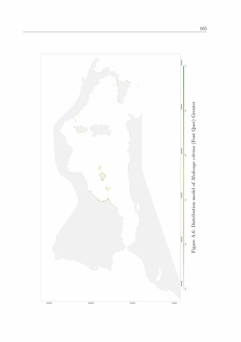
165
Fig
ure
A.6
:D
istr
ibuti
onm
odel
ofM
edic
ago
citr
ina
(Fon
tQ
uer
)G
reute
r

166 APPENDIX A. DISTRIBUTION MODEL MAPS OF SCI
Fig
ure
A.7
:D
istr
ibuti
onm
odel
ofS
ilen
ehi
face
nsi
sR
ouy
exW
illk
.

Appendix B
Protected range maps of Species of
Conservation Interest
167

168 APPENDIX B. PROTECTED RANGE MAPS OF SCI
Fig
ure
B.1
:A
sple
niu
mm
ajor
icu
mpro
tect
edra
nge
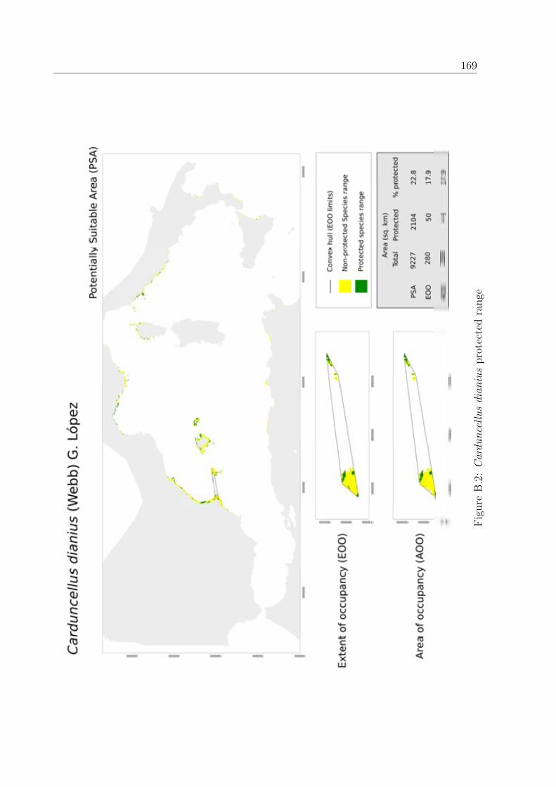
169
Fig
ure
B.2
:C
ardu
nce
llu
sdi
aniu
spro
tect
edra
nge
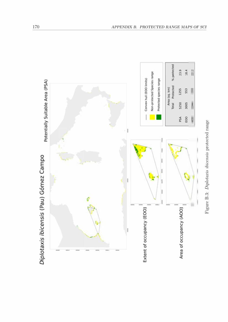
170 APPENDIX B. PROTECTED RANGE MAPS OF SCI
Fig
ure
B.3
:D
iplo
taxi
sib
icen
sis
pro
tect
edra
nge

171
Fig
ure
B.4
:E
uph
orbi
asq
uam
iger
apro
tect
edra
nge
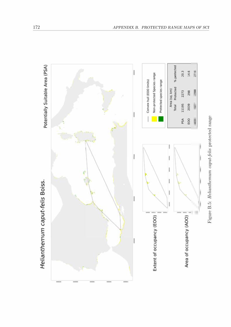
172 APPENDIX B. PROTECTED RANGE MAPS OF SCI
Fig
ure
B.5
:H
elia
nth
emu
mca
put-
feli
spro
tect
edra
nge

173
Fig
ure
B.6
:M
edic
ago
citr
ina
pro
tect
edra
nge

174 APPENDIX B. PROTECTED RANGE MAPS OF SCI
Fig
ure
B.7
:S
ilen
ehi
face
nsi
spro
tect
edra
nge

Appendix C
Protected range sizes of Species of
Conservation Interest
How to interpret these results All calculations were done at 1-km resolution. A land
mask was used in order to exclude sea pixels. In this mask, all 1-km grid cells that inter-
sected with land where considered as land, however small its intersection was. Marine-only
sites may appear in the tables since, at coastal areas, many 1-km grid cells share land and
sea (besides, in the Natura 2000 shape�le, marine sites are not individualized and many
sites are a single polygon comprising terrestrial and marine areas). Since all 1-km cells
intersecting any given protected site are considered, the 'PA cells' column in each table
shows an area in square km which is always greater than the actual site area. Results are
grouped per species and there are up to four tables per species. However, some tables may
be missing depending on the species' range maps:
Tables of Potentially Suitable Areas protection by Natura 2000 protected ar-
eas.
These tables provides the results of overlaying the Potentially Suitable
Areas (PSA), as de�ned in the article, with the Natura 2000 sites.
Columns: Code: Natura 2000 o�cial site code (�eld 'SITECODE' in
Natura 2000 shape�le), Name: Natura 2000 o�cial site name (�eld
175

176 APPENDIX C. PROTECTED RANGE SIZES OF SCI
'SITENAME' in Natura 2000 shape�le), PA cells: Number of 1 km cells
which intersect with the site polygon, PSA cells: Number of suitable 1
km cells which intersect with the site polygon, Perc. PSA: Percentage
of 'PSA cells' with respect to 'PA cells'.
Tables of Species EOO and AOO protection by Natura 2000 protected areas.
These tables provide the results of overlaying the Extent of Occurrence
(EOO) and Area of Occupancy (AOO), as de�ned in the article, with
the Natura 2000 sites.
Columns: Code: Natura 2000 o�cial site code (�eld 'SITECODE' in
Natura 2000 shape�le), Name: Natura 2000 o�cial site name (�eld
'SITENAME' in Natura 2000 shape�le), PA cells: Number of 1 km cells
which intersect with the site polygon, EOO cells: Number of 1 km cells
which intersect with the species' EOO polygon (sea excluded) and with
the site polygon, Perc. EOO: Percentage of 'EOO cells' with respect
to 'PA cells', AOO cells: Number of 1 km cells which intersect with
the species' AOO (as de�ned in the article) and with the site polygon,
Perc. AOO: Percentage of 'AOO cells' with respect to 'PA cells'.
Tables of Potentially Suitable Areas protection by North African protected
areas.
These tables provide the results of overlaying the PSA, as de�ned in the
article, with the protected areas of North Africa.
Columns: Code: Site's identi�cation code (�eld 'wdpaid') in the World
Database of Protected Areas (WDPA), Type: Protection category (�eld
'desig eng') in the WDPA, Name: Site name (�eld 'name') in the WDPA,
PA cells: Number of 1 km cells which intersect with the site polygon,
PSA cells: Number of suitable 1 km cells which intersect with the site
polygon, Perc. PSA: Percentage of 'PSA cells' with respect to 'PA cells'.
Tables of Species EOO and AOO protection by North African protected areas.
177
These tables provides the results of overlaying the EOO and AOO, as
de�ned in the article, with the protected areas of North Africa.
Columns: Code: Site's identi�cation code (�eld 'wdpaid') in the World
Database of Protected Areas (WDPA), Type: Protection category (�eld
'desig eng') in the WDPA, Name: Site name (�eld 'name') in the WDPA
PA cells: Number of 1 km cells which intersect with the site polygon,
EOO cells: Number of 1 km cells which intersect with the species'
EOO polygon (sea excluded) and with the site polygon, Perc. EOO:
Percentage of 'EOO cells' with respect to 'PA cells', AOO cells: Number
of 1 km cells which intersect with the species' AOO (as de�ned in the
article) and with the site polygon, Perc. AOO: Percentage of 'AOO
cells' with respect to 'PA cells'.
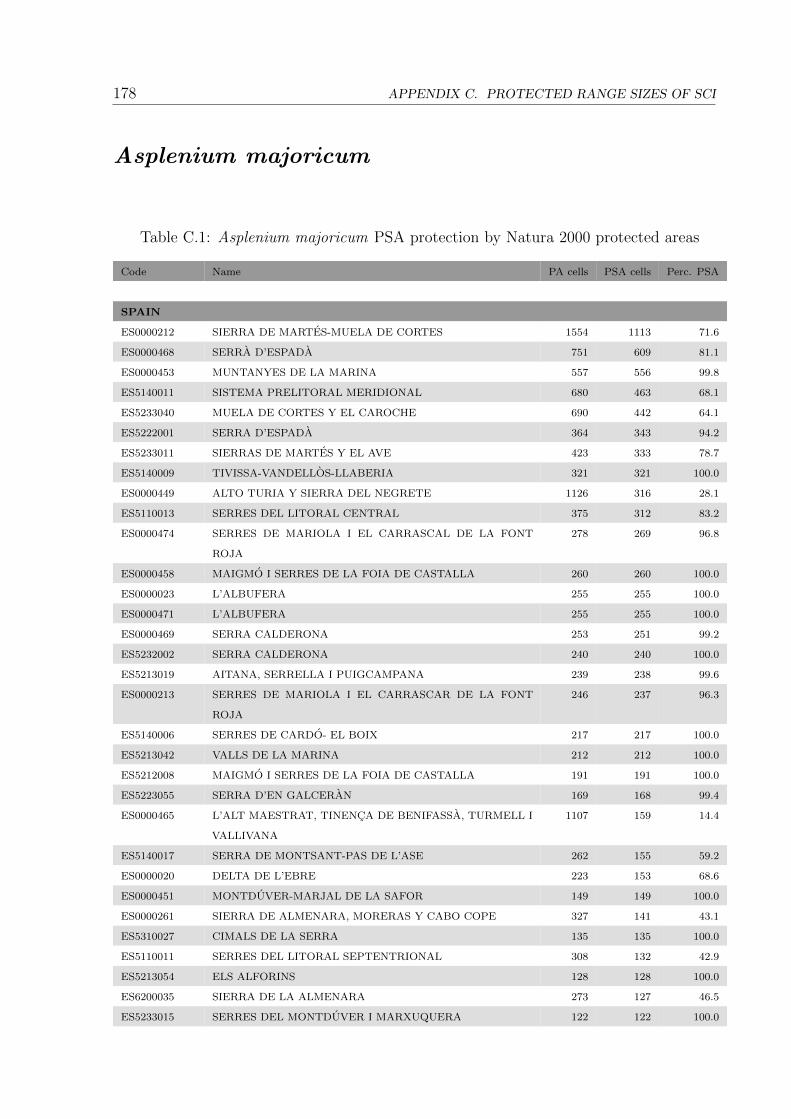
178 APPENDIX C. PROTECTED RANGE SIZES OF SCI
Asplenium majoricum
Table C.1: Asplenium majoricum PSA protection by Natura 2000 protected areas
Code Name PA cells PSA cells Perc. PSA
SPAIN
ES0000212 SIERRA DE MARTES-MUELA DE CORTES 1554 1113 71.6
ES0000468 SERRA D’ESPADA 751 609 81.1
ES0000453 MUNTANYES DE LA MARINA 557 556 99.8
ES5140011 SISTEMA PRELITORAL MERIDIONAL 680 463 68.1
ES5233040 MUELA DE CORTES Y EL CAROCHE 690 442 64.1
ES5222001 SERRA D’ESPADA 364 343 94.2
ES5233011 SIERRAS DE MARTES Y EL AVE 423 333 78.7
ES5140009 TIVISSA-VANDELLOS-LLABERIA 321 321 100.0
ES0000449 ALTO TURIA Y SIERRA DEL NEGRETE 1126 316 28.1
ES5110013 SERRES DEL LITORAL CENTRAL 375 312 83.2
ES0000474 SERRES DE MARIOLA I EL CARRASCAL DE LA FONT
ROJA
278 269 96.8
ES0000458 MAIGMO I SERRES DE LA FOIA DE CASTALLA 260 260 100.0
ES0000023 L’ALBUFERA 255 255 100.0
ES0000471 L’ALBUFERA 255 255 100.0
ES0000469 SERRA CALDERONA 253 251 99.2
ES5232002 SERRA CALDERONA 240 240 100.0
ES5213019 AITANA, SERRELLA I PUIGCAMPANA 239 238 99.6
ES0000213 SERRES DE MARIOLA I EL CARRASCAR DE LA FONT
ROJA
246 237 96.3
ES5140006 SERRES DE CARDO- EL BOIX 217 217 100.0
ES5213042 VALLS DE LA MARINA 212 212 100.0
ES5212008 MAIGMO I SERRES DE LA FOIA DE CASTALLA 191 191 100.0
ES5223055 SERRA D’EN GALCERAN 169 168 99.4
ES0000465 L’ALT MAESTRAT, TINENCA DE BENIFASSA, TURMELL I
VALLIVANA
1107 159 14.4
ES5140017 SERRA DE MONTSANT-PAS DE L’ASE 262 155 59.2
ES0000020 DELTA DE L’EBRE 223 153 68.6
ES0000451 MONTDUVER-MARJAL DE LA SAFOR 149 149 100.0
ES0000261 SIERRA DE ALMENARA, MORERAS Y CABO COPE 327 141 43.1
ES5310027 CIMALS DE LA SERRA 135 135 100.0
ES5110011 SERRES DEL LITORAL SEPTENTRIONAL 308 132 42.9
ES5213054 ELS ALFORINS 128 128 100.0
ES6200035 SIERRA DE LA ALMENARA 273 127 46.5
ES5233015 SERRES DEL MONTDUVER I MARXUQUERA 122 122 100.0
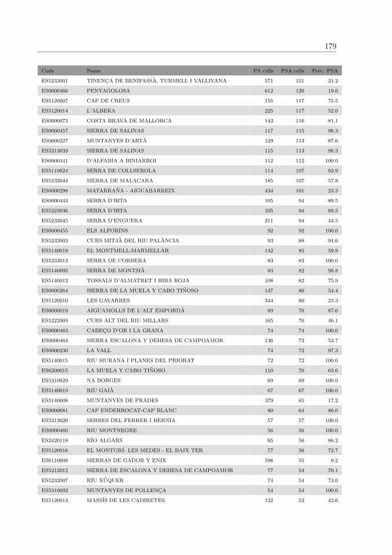
179
Code Name PA cells PSA cells Perc. PSA
ES5233001 TINENCA DE BENIFASSA, TURMELL I VALLIVANA 571 121 21.2
ES0000466 PENYAGOLOSA 612 120 19.6
ES5120007 CAP DE CREUS 155 117 75.5
ES5120014 L’ALBERA 225 117 52.0
ES0000073 COSTA BRAVA DE MALLORCA 143 116 81.1
ES0000457 SIERRA DE SALINAS 117 115 98.3
ES0000227 MUNTANYES D’ARTA 129 113 87.6
ES5213039 SIERRA DE SALINAS 115 113 98.3
ES0000441 D’ALFABIA A BINIARROI 112 112 100.0
ES5110024 SERRA DE COLLSEROLA 114 107 93.9
ES5233044 SIERRA DE MALACARA 185 107 57.8
ES0000298 MATARRANA - AIGUABARREIX 434 101 23.3
ES0000444 SERRA D’IRTA 105 94 89.5
ES5223036 SERRA D’IRTA 105 94 89.5
ES5233045 SERRA D’ENGUERA 211 94 44.5
ES0000455 ELS ALFORINS 92 92 100.0
ES5232003 CURS MITJA DEL RIU PALANCIA 93 88 94.6
ES5140018 EL MONTMELL-MARMELLAR 142 85 59.9
ES5233013 SERRA DE CORBERA 83 83 100.0
ES5140005 SERRA DE MONTSIA 83 82 98.8
ES5140012 TOSSALS D’ALMATRET I RIBA ROJA 108 82 75.9
ES0000264 SIERRA DE LA MUELA Y CABO TINOSO 147 80 54.4
ES5120010 LES GAVARRES 344 80 23.3
ES0000019 AIGUAMOLLS DE L’ALT EMPORDA 89 78 87.6
ES5222004 CURS ALT DEL RIU MILLARS 165 76 46.1
ES0000463 CABECO D’OR I LA GRANA 74 74 100.0
ES0000464 SIERRA ESCALONA Y DEHESA DE CAMPOAMOR 136 73 53.7
ES0000230 LA VALL 74 72 97.3
ES5140015 RIU SIURANA I PLANES DEL PRIORAT 72 72 100.0
ES6200015 LA MUELA Y CABO TINOSO 110 70 63.6
ES5310029 NA BORGES 69 69 100.0
ES5140019 RIU GAIA 67 67 100.0
ES5140008 MUNTANYES DE PRADES 379 65 17.2
ES0000081 CAP ENDERROCAT-CAP BLANC 80 64 80.0
ES5213020 SERRES DEL FERRER I BERNIA 57 57 100.0
ES0000460 RIU MONTNEGRE 56 56 100.0
ES2420118 RIO ALGARS 65 56 86.2
ES5120016 EL MONTGRI- LES MEDES - EL BAIX TER 77 56 72.7
ES6110008 SIERRAS DE GADOR Y ENIX 598 55 9.2
ES5212012 SIERRA DE ESCALONA Y DEHESA DE CAMPOAMOR 77 54 70.1
ES5232007 RIU XUQUER 74 54 73.0
ES5310092 MUNTANYES DE POLLENCA 54 54 100.0
ES5120013 MASSIS DE LES CADIRETES 122 52 42.6

180 APPENDIX C. PROTECTED RANGE SIZES OF SCI
Code Name PA cells PSA cells Perc. PSA
ES0000228 CAP DE SES SALINES 60 51 85.0
ES5140003 RIBERA DE L’ALGARS 51 50 98.0
ES0000231 DELS ALOCS A FORNELLS 52 49 94.2
ES5233041 SERRA DE LA SAFOR 49 49 100.0
ES0000446 DESERT DE LES PALMES 48 48 100.0
ES0000084 SES SALINES D’EIVISSA I FORMENTERA 76 47 61.8
ES5221002 DESERT DE LES PALMES 47 47 100.0
ES5233009 SIERRA DEL NEGRETE 285 47 16.5
ES0000461 SERRES DEL SUD D’ALACANT 142 46 32.4
ES5140023 SECANS DEL MONTSIA 46 46 100.0
ES5310032 CAP LLENTRISCA-SA TALAIA 50 46 92.0
ES0000059 LLACUNES DE LA MATA I TORREVIEJA. 60 45 75.0
ES5140014 MASSIS DE BONASTRE 45 45 100.0
ES5213022 SERRA DE CREVILLENT 78 45 57.7
ES0000173 SIERRA ESPUNA 223 44 19.7
ES5310113 LA VALL 46 44 95.7
ES0000083 ARXIPELAG DE CABRERA 75 42 56.0
ES0000237 DES CANUTELLS A LLUCALARI 45 42 93.3
ES0000120 SALINAS DE SANTA POLA. 44 41 93.2
ES0000239 DE BINIGAUS A CALA MITJANA 48 41 85.4
ES0000445 PLANIOLS-BENASQUES 38 38 100.0
ES0000454 MONTGO-CAP DE SANT ANTONI 40 37 92.5
ES5211007 MONTGO 40 37 92.5
ES0000038 S’ALBUFERA DE MALLORCA 39 36 92.3
ES5310008 ES GALATZO-S’ESCLOP 36 36 100.0
ES0000443 SUD DE CIUTADELLA 38 35 92.1
ES6200001 CALBLANQUE, MONTE DE LAS CENIZAS Y PENA DEL
AGUILA
52 35 67.3
ES6200009 SIERRA DE EL CARCHE 86 35 40.7
ES0000442 DE LA SERRA DE L’ESPERO AL PENYAL ALT 34 34 100.0
ES5140002 SERRA DE GODALL 34 34 100.0
ES5310079 PUIG DE NA BAUCA 34 34 100.0
ES5310105 ES AMUNTS D’EIVISSA 36 33 91.7
ES0000440 DES TEIX AL PUIG DE SES FITES 32 32 100.0
ES0000450 MARJAL I ESTANYS D’ALMENARA 32 32 100.0
ES5140010 RIBERES I ILLES DE L’EBRE 32 32 100.0
ES5223007 MARJAL D’ALMENARA 32 32 100.0
ES0000235 DE S’ALBUFERA A LA MOLA 41 31 75.6
ES0000386 CAPELL DE FERRO 30 30 100.0
ES0000238 SON BOU I BARRANC DE SA VALL 29 28 96.6
ES0000260 MAR MENOR 67 28 41.8
ES5140016 TOSSAL DE MONTAGUT 28 28 100.0
ES5310035 AREA MARINA DEL NORD DE MENORCA 34 28 82.4
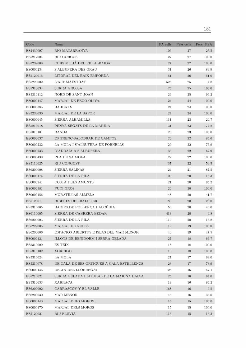
181
Code Name PA cells PSA cells Perc. PSA
ES2430097 RIO MATARRANYA 106 27 25.5
ES5212004 RIU GORGOS 27 27 100.0
ES5232008 CURS MITJA DEL RIU ALBAIDA 27 27 100.0
ES0000234 S’ALBUFERA DES GRAU 31 26 83.9
ES5120015 LITORAL DEL BAIX EMPORDA 51 26 51.0
ES5223002 L’ALT MAESTRAT 525 25 4.8
ES5310034 SERRA GROSSA 25 25 100.0
ES5310112 NORD DE SANT JOAN 26 25 96.2
ES0000147 MARJAL DE PEGO-OLIVA. 24 24 100.0
ES0000385 BARBATX 24 24 100.0
ES5233030 MARJAL DE LA SAFOR 24 24 100.0
ES0000045 SIERRA ALHAMILLA 111 23 20.7
ES5213018 PENYA-SEGATS DE LA MARINA 31 23 74.2
ES5310101 RANDA 23 23 100.0
ES0000037 ES TRENC-SALOBRAR DE CAMPOS 26 22 84.6
ES0000232 LA MOLA I S’ALBUFERA DE FORNELLS 29 22 75.9
ES0000233 D’ADDAIA A S’ALBUFERA 35 22 62.9
ES0000439 PLA DE SA MOLA 22 22 100.0
ES5110025 RIU CONGOST 37 22 59.5
ES6200008 SIERRA SALINAS 24 21 87.5
ES0000174 SIERRA DE LA PILA 109 20 18.3
ES0000241 COSTA DELS AMUNTS 21 20 95.2
ES0000381 PUIG GROS 20 20 100.0
ES0000456 MORATILLAS-ALMELA 48 20 41.7
ES5120011 RIBERES DEL BAIX TER 80 20 25.0
ES5310005 BADIES DE POLLENCA I ALCUDIA 50 20 40.0
ES6110005 SIERRA DE CABRERA-BEDAR 413 20 4.8
ES6200003 SIERRA DE LA PILA 119 20 16.8
ES5222005 MARJAL DE NULES 19 19 100.0
ES6200006 ESPACIOS ABIERTOS E ISLAS DEL MAR MENOR 40 19 47.5
ES0000121 ILLOTS DE BENIDORM I SERRA GELADA 27 18 66.7
ES5310009 ES TEIX 18 18 100.0
ES5310102 XORRIGO 18 18 100.0
ES5310024 LA MOLA 27 17 63.0
ES5310078 DE CALA DE SES ORTIGUES A CALA ESTELLENCS 23 17 73.9
ES0000146 DELTA DEL LLOBREGAT 28 16 57.1
ES5213021 SERRA GELADA I LITORAL DE LA MARINA BAIXA 25 16 64.0
ES5310033 XARRACA 19 16 84.2
ES6200002 CARRASCOY Y EL VALLE 168 16 9.5
ES6200030 MAR MENOR 45 16 35.6
ES0000148 MARJAL DELS MOROS. 15 15 100.0
ES0000470 MARJAL DELS MOROS 15 15 100.0
ES5120021 RIU FLUVIA 113 15 13.3
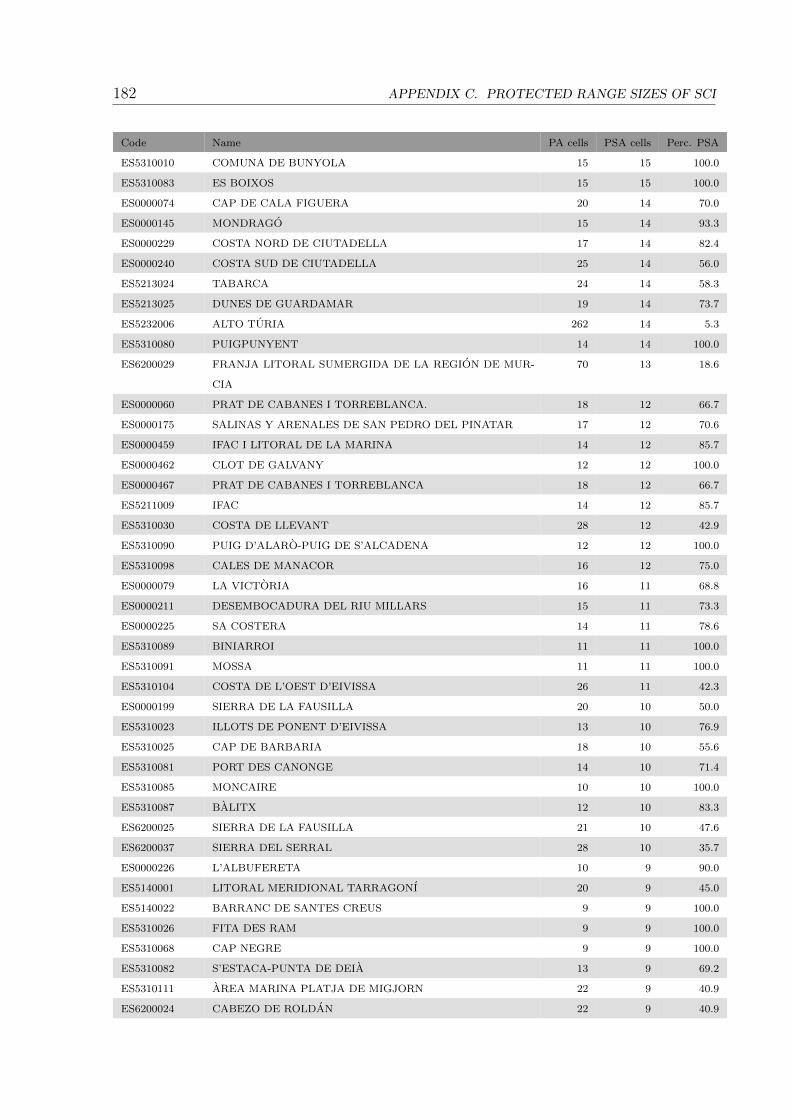
182 APPENDIX C. PROTECTED RANGE SIZES OF SCI
Code Name PA cells PSA cells Perc. PSA
ES5310010 COMUNA DE BUNYOLA 15 15 100.0
ES5310083 ES BOIXOS 15 15 100.0
ES0000074 CAP DE CALA FIGUERA 20 14 70.0
ES0000145 MONDRAGO 15 14 93.3
ES0000229 COSTA NORD DE CIUTADELLA 17 14 82.4
ES0000240 COSTA SUD DE CIUTADELLA 25 14 56.0
ES5213024 TABARCA 24 14 58.3
ES5213025 DUNES DE GUARDAMAR 19 14 73.7
ES5232006 ALTO TURIA 262 14 5.3
ES5310080 PUIGPUNYENT 14 14 100.0
ES6200029 FRANJA LITORAL SUMERGIDA DE LA REGION DE MUR-
CIA
70 13 18.6
ES0000060 PRAT DE CABANES I TORREBLANCA. 18 12 66.7
ES0000175 SALINAS Y ARENALES DE SAN PEDRO DEL PINATAR 17 12 70.6
ES0000459 IFAC I LITORAL DE LA MARINA 14 12 85.7
ES0000462 CLOT DE GALVANY 12 12 100.0
ES0000467 PRAT DE CABANES I TORREBLANCA 18 12 66.7
ES5211009 IFAC 14 12 85.7
ES5310030 COSTA DE LLEVANT 28 12 42.9
ES5310090 PUIG D’ALARO-PUIG DE S’ALCADENA 12 12 100.0
ES5310098 CALES DE MANACOR 16 12 75.0
ES0000079 LA VICTORIA 16 11 68.8
ES0000211 DESEMBOCADURA DEL RIU MILLARS 15 11 73.3
ES0000225 SA COSTERA 14 11 78.6
ES5310089 BINIARROI 11 11 100.0
ES5310091 MOSSA 11 11 100.0
ES5310104 COSTA DE L’OEST D’EIVISSA 26 11 42.3
ES0000199 SIERRA DE LA FAUSILLA 20 10 50.0
ES5310023 ILLOTS DE PONENT D’EIVISSA 13 10 76.9
ES5310025 CAP DE BARBARIA 18 10 55.6
ES5310081 PORT DES CANONGE 14 10 71.4
ES5310085 MONCAIRE 10 10 100.0
ES5310087 BALITX 12 10 83.3
ES6200025 SIERRA DE LA FAUSILLA 21 10 47.6
ES6200037 SIERRA DEL SERRAL 28 10 35.7
ES0000226 L’ALBUFERETA 10 9 90.0
ES5140001 LITORAL MERIDIONAL TARRAGONI 20 9 45.0
ES5140022 BARRANC DE SANTES CREUS 9 9 100.0
ES5310026 FITA DES RAM 9 9 100.0
ES5310068 CAP NEGRE 9 9 100.0
ES5310082 S’ESTACA-PUNTA DE DEIA 13 9 69.2
ES5310111 AREA MARINA PLATJA DE MIGJORN 22 9 40.9
ES6200024 CABEZO DE ROLDAN 22 9 40.9
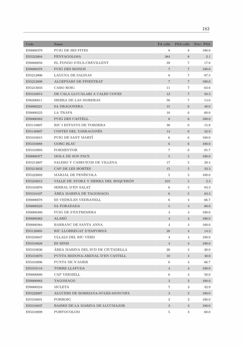
183
Code Name PA cells PSA cells Perc. PSA
ES0000379 PUIG DE SES FITES 8 8 100.0
ES5223004 PENYAGOLOSA 384 8 2.1
ES0000058 EL FONDO D’ELX-CREVILLENT 39 7 17.9
ES0000378 PUIG DES BOIXOS 7 7 100.0
ES5212006 LAGUNA DE SALINAS 8 7 87.5
ES5212009 ALGEPSARS DE FINESTRAT 7 7 100.0
ES5213033 CABO ROIG 11 7 63.6
ES5310074 DE CALA LLUCALARI A CALES COVES 12 7 58.3
ES6200011 SIERRA DE LAS MORERAS 50 7 14.0
ES0000221 SA DRAGONERA 15 6 40.0
ES0000222 LA TRAPA 10 6 60.0
ES0000383 PUIG DES CASTELL 6 6 100.0
ES5110007 RIU I ESTANYS DE TORDERA 38 6 15.8
ES5140007 COSTES DEL TARRAGONES 14 6 42.9
ES5310015 PUIG DE SANT MARTI 6 6 100.0
ES5310088 GORG BLAU 6 6 100.0
ES5310093 FORMENTOR 7 6 85.7
ES0000377 MOLA DE SON PACS 5 5 100.0
ES5212007 SALERO Y CABECICOS DE VILLENA 17 5 29.4
ES5213032 CAP DE LES HORTES 15 5 33.3
ES5222002 MARJAL DE PENISCOLA 5 5 100.0
ES5233012 VALLE DE AYORA Y SIERRA DEL BOQUERON 219 5 2.3
ES5310076 SERRAL D’EN SALAT 6 5 83.3
ES5310107 AREA MARINA DE TAGOMAGO 6 5 83.3
ES0000078 ES VEDRA-ES VEDRANELL 6 4 66.7
ES0000223 SA FORADADA 5 4 80.0
ES0000380 PUIG DE S’EXTREMERA 4 4 100.0
ES0000382 ALARO 4 4 100.0
ES0000384 BARRANC DE SANTA ANNA 4 4 100.0
ES5120005 RIU LLOBREGAT D’EMPORDA 28 4 14.3
ES5233047 ULLALS DEL RIU VERD 4 4 100.0
ES5310028 ES BINIS 4 4 100.0
ES5310036 AREA MARINA DEL SUD DE CIUTADELLA 20 4 20.0
ES5310070 PUNTA REDONA-ARENAL D’EN CASTELL 10 4 40.0
ES5310096 PUNTA DE N’AMER 6 4 66.7
ES5310118 TORRE LLAFUDA 4 4 100.0
ES0000080 CAP VERMELL 6 3 50.0
ES0000082 TAGOMAGO 3 3 100.0
ES0000224 MULETA 7 3 42.9
ES5222007 ALGUERS DE BORRIANA-NULES-MONCOFA 3 3 100.0
ES5310031 PORROIG 3 3 100.0
ES5310037 BASSES DE LA MARINA DE LLUCMAJOR 3 3 100.0
ES5310099 PORTOCOLOM 5 3 60.0

184 APPENDIX C. PROTECTED RANGE SIZES OF SCI
Code Name PA cells PSA cells Perc. PSA
ES5310109 AREA MARINA DE CALA SAONA 4 3 75.0
ES5310119 PENYES D’EGIPTE 3 3 100.0
ES5310120 ES CLOT DES GUIX 3 3 100.0
ES5310122 MAL LLOC 3 3 100.0
ES6200012 CALNEGRE 18 3 16.7
ES6200048 MEDIO MARINO 15 3 20.0
ES0000061 ILLES COLUMBRETES 4 2 50.0
ES0000214 ILLOTS DE TABARCA 12 2 16.7
ES5110020 COSTES DEL GARRAF 12 2 16.7
ES5140004 SEQUIA MAJOR 4 2 50.0
ES5223005 ALT PALANCIA 314 2 0.6
ES5310069 CALA D’ALGAIRENS 3 2 66.7
ES5310084 TORRE PICADA 5 2 40.0
ES5310086 MONNABER 2 2 100.0
ES5310106 AREA MARINA DE SES MARGALIDES 2 2 100.0
ES5310108 AREA MARINA DEL CAP MARTINET 7 2 28.6
ES5310114 BINIGAFULL 2 2 100.0
ES5310115 ES MOLINET 2 2 100.0
ES5310121 BINIGURDO 2 2 100.0
ES6110006 RAMBLAS DE GERGAL, TABERNAS Y SUR DE SIERRA AL-
HAMILLA
324 2 0.6
ES6200023 SIERRA DE LA TERCIA 73 2 2.7
ES0000307 PUERTOS DE BECEITE 189 1 0.5
ES0000447 COSTA D’ORPESA I BENICASSIM 6 1 16.7
ES2420119 ELS PORTS DE BESEIT 138 1 0.7
ES5110015 SISTEMA PRELITORAL CENTRAL 293 1 0.3
ES5140020 GRAPISSAR DE LA MASIA BLANCA 4 1 25.0
ES5212010 ARENAL DE PETRER 1 1 100.0
ES5214002 TUNEL DE CANALS 1 1 100.0
ES5214004 COVA JOLIANA 1 1 100.0
ES5222006 PLATJA DE MONCOFA 1 1 100.0
ES5223037 COSTA D’ORPESA I BENICASSIM 6 1 16.7
ES5224001 COVA OSCURA-ATZENETA DEL MAESTRAT 1 1 100.0
ES5232009 SERRA DEL CASTELL DE XATIVA 1 1 100.0
ES5233049 COVA DE LES RATES PENADES (ROTOVA) 1 1 100.0
ES5233051 COVA DE LES MERAVELLES DE LLOMBAI 1 1 100.0
ES5234001 COVA DEL SARDINER-SAGUNT 1 1 100.0
ES5234005 SIMA DE L’AGUILA-PICASSENT 1 1 100.0
ES5310040 COVA DE LES MARAVELLES 1 1 100.0
ES5310042 AVENC D’EN CORBERA 1 1 100.0
ES5310048 COVA DE SA GUITARRETA 1 1 100.0
ES5310050 COVA D’EN BESSO 1 1 100.0
ES5310055 COVA DES PIRATA 1 1 100.0

185
Code Name PA cells PSA cells Perc. PSA
ES5310056 COVA DES PONT 1 1 100.0
ES5310057 COVA DE CAL PESSO 1 1 100.0
ES5310058 COVA DE CAN SION 1 1 100.0
ES5310059 COVA DE LLENAIRE 1 1 100.0
ES5310060 COVA MORELLA 1 1 100.0
ES5310061 COVA NOVA DE SON LLUIS 1 1 100.0
ES5310062 ES BUFADOR DE SON BERENGUER 1 1 100.0
ES5310063 COVA DE CAN MILLO O DE COA NEGRINA 1 1 100.0
ES5310064 AVENC DE SON POU 1 1 100.0
ES5310072 CALETA DE BINILLAUTI 1 1 100.0
ES5310075 ARENAL DE SON SAURA 5 1 20.0
ES5310095 CAN PICAFORT 3 1 33.3
ES5310100 PUNTA DES RAS 2 1 50.0
ES5310116 BINIATRUM 1 1 100.0
ES5310117 SES PALLISSES 1 1 100.0
ES5310123 BASSA DE FORMENTERA 1 1 100.0
ES6200027 SIERRA DE ABANILLA 23 1 4.3
SPAIN TOTAL: 28261 15904 56.3
FRANCE
FR9310019 CAMARGUE 899 697 77.5
FR9301592 CAMARGUE 884 686 77.6
FR9301622 LA PLAINE ET LE MASSIF DES MAURES 450 414 92.0
FR9301595 CRAU CENTRALE - CRAU SECHE 525 376 71.6
FR9310064 CRAU 493 362 73.4
FR9101406 PETITE CAMARGUE 405 310 76.5
FR9112013 PETITE CAMARGUE LAGUNO-MARINE 208 186 89.4
FR9400577 RIVIERE ET VALLEE DU FANGO 249 142 57.0
FR9400574 PORTO/SCANDOLA/REVELLATA/CALVI/CALANCHES
DE PIANA (ZONE TERRESTRE ET MARINE)
202 135 66.8
FR9410023 GOLFE DE PORTO ET PRESQU’ILE DE SCANDOLA 181 133 73.5
FR9310069 GARRIGUES DE LANCON ET CHAINES ALENTOUR 348 132 37.9
FR9301608 MONT CAUME - MONT FARON - FORET DOMANIALE DES
MORIERES
171 130 76.0
FR9301603 CHAINE DE L’ETOILE- MASSIF DU GARLABAN 139 127 91.4
FR9112007 ETANGS DU NARBONNAIS 142 122 85.9
FR9400570 AGRIATES 151 119 78.8
FR9110080 MONTAGNE DE LA CLAPE 120 106 88.3
FR9301628 ESTEREL 124 106 85.5
FR9101453 MASSIF DE LA CLAPE 113 105 92.9
FR9301596 MARAIS DE LA VALLEE DES BAUX ET MARAIS D’ARLES 189 104 55.0
FR9112018 ETANG DE THAU ET LIDO DE SETE A AGDE 110 98 89.1
FR9312001 MARAIS ENTRE CRAU ET GRAND RHONE 110 94 85.5
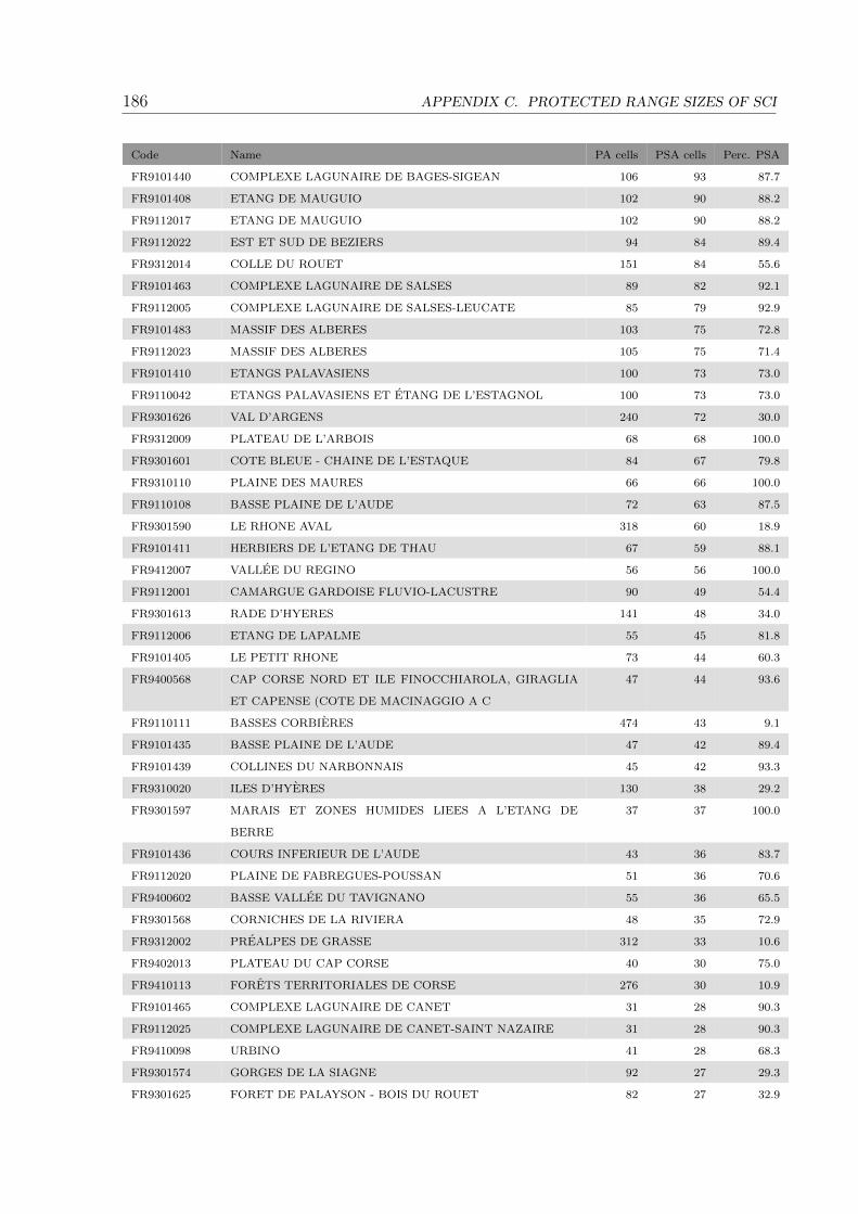
186 APPENDIX C. PROTECTED RANGE SIZES OF SCI
Code Name PA cells PSA cells Perc. PSA
FR9101440 COMPLEXE LAGUNAIRE DE BAGES-SIGEAN 106 93 87.7
FR9101408 ETANG DE MAUGUIO 102 90 88.2
FR9112017 ETANG DE MAUGUIO 102 90 88.2
FR9112022 EST ET SUD DE BEZIERS 94 84 89.4
FR9312014 COLLE DU ROUET 151 84 55.6
FR9101463 COMPLEXE LAGUNAIRE DE SALSES 89 82 92.1
FR9112005 COMPLEXE LAGUNAIRE DE SALSES-LEUCATE 85 79 92.9
FR9101483 MASSIF DES ALBERES 103 75 72.8
FR9112023 MASSIF DES ALBERES 105 75 71.4
FR9101410 ETANGS PALAVASIENS 100 73 73.0
FR9110042 ETANGS PALAVASIENS ET ETANG DE L’ESTAGNOL 100 73 73.0
FR9301626 VAL D’ARGENS 240 72 30.0
FR9312009 PLATEAU DE L’ARBOIS 68 68 100.0
FR9301601 COTE BLEUE - CHAINE DE L’ESTAQUE 84 67 79.8
FR9310110 PLAINE DES MAURES 66 66 100.0
FR9110108 BASSE PLAINE DE L’AUDE 72 63 87.5
FR9301590 LE RHONE AVAL 318 60 18.9
FR9101411 HERBIERS DE L’ETANG DE THAU 67 59 88.1
FR9412007 VALLEE DU REGINO 56 56 100.0
FR9112001 CAMARGUE GARDOISE FLUVIO-LACUSTRE 90 49 54.4
FR9301613 RADE D’HYERES 141 48 34.0
FR9112006 ETANG DE LAPALME 55 45 81.8
FR9101405 LE PETIT RHONE 73 44 60.3
FR9400568 CAP CORSE NORD ET ILE FINOCCHIAROLA, GIRAGLIA
ET CAPENSE (COTE DE MACINAGGIO A C
47 44 93.6
FR9110111 BASSES CORBIERES 474 43 9.1
FR9101435 BASSE PLAINE DE L’AUDE 47 42 89.4
FR9101439 COLLINES DU NARBONNAIS 45 42 93.3
FR9310020 ILES D’HYERES 130 38 29.2
FR9301597 MARAIS ET ZONES HUMIDES LIEES A L’ETANG DE
BERRE
37 37 100.0
FR9101436 COURS INFERIEUR DE L’AUDE 43 36 83.7
FR9112020 PLAINE DE FABREGUES-POUSSAN 51 36 70.6
FR9400602 BASSE VALLEE DU TAVIGNANO 55 36 65.5
FR9301568 CORNICHES DE LA RIVIERA 48 35 72.9
FR9312002 PREALPES DE GRASSE 312 33 10.6
FR9402013 PLATEAU DU CAP CORSE 40 30 75.0
FR9410113 FORETS TERRITORIALES DE CORSE 276 30 10.9
FR9101465 COMPLEXE LAGUNAIRE DE CANET 31 28 90.3
FR9112025 COMPLEXE LAGUNAIRE DE CANET-SAINT NAZAIRE 31 28 90.3
FR9410098 URBINO 41 28 68.3
FR9301574 GORGES DE LA SIAGNE 92 27 29.3
FR9301625 FORET DE PALAYSON - BOIS DU ROUET 82 27 32.9

187
Code Name PA cells PSA cells Perc. PSA
FR9312015 ETANGS ENTRE ISTRES ET FOS 28 26 92.9
FR9412009 PLATEAU DU CAP CORSE 32 26 81.2
FR9112008 CORBIERES ORIENTALES 311 25 8.0
FR9301571 RIVIERE ET GORGES DU LOUP 84 24 28.6
FR9410097 ILES FINOCCHIAROLA ET COTE NORD 27 24 88.9
FR9312025 BASSE VALLEE DU VAR 31 23 74.2
FR9400571 ETANG DE BIGUGLIA 37 23 62.2
FR9301567 VALLEE DU CARAI - COLLINES DE CASTILLON 73 22 30.1
FR9410101 ETANG DE BIGUGLIA 35 22 62.9
FR9412010 CAPU ROSSU , SCANDOLA, REVELLATA, CALVI 40 22 55.0
FR9101441 COMPLEXE LAGUNAIRE DE LAPALME 31 21 67.7
FR9112021 PLAINE DE VILLEVEYRAC-MONTAGNAC 74 20 27.0
FR9301627 EMBOUCHURE DE L’ARGENS 24 20 83.3
FR9101486 COURS INFERIEUR DE L’HERAULT 21 19 90.5
FR9301569 VALLONS OBSCURS DE NICE ET DE SAINT BLAISE 28 19 67.9
FR9101478 LE TECH 79 17 21.5
FR9101481 COTE ROCHEUSE DES ALBERES 28 17 60.7
FR9400603 RIVIERE DE LA SOLENZARA 65 17 26.2
FR9312008 SALINS D’HYERES ET DES PESQUIERS 21 16 76.2
FR9402017 GOLFE D’AJACCIO 66 16 24.2
FR9410096 ILES SANGUINAIRES, GOLFE D’AJACCIO 66 16 24.2
FR9402012 CAPO DI FENO 29 15 51.7
FR9402018 CAP ROSSU, SCANDOLA, POINTE DE LA REVELETTA,
CANYON DE CALVI
25 14 56.0
FR9312005 SALINES DE L’ETANG DE BERRE 11 11 100.0
FR9400580 MARAIS DEL SALE, ZONES HUMIDES PERIPHERIQUES ET
FORET LITTORALE DE PINIA
22 11 50.0
FR9101412 ETANG DU BAGNAS 13 10 76.9
FR9110034 ETANG DU BAGNAS 12 10 83.3
FR9301610 CAP SICIE - SIX FOURS 18 10 55.6
FR9101391 LE VIDOURLE 30 9 30.0
FR9400601 ALISO-OLETTA 9 9 100.0
FR9101493 EMBOUCHURE DU TECH ET GRAU DE LA MASSANE 14 8 57.1
FR9112034 CAP BEAR- CAP CERBERE 16 8 50.0
FR9400572 MUCCHIATANA 9 8 88.9
FR9400598 MASSIF DU TENDA ET FORET DE STELLA 52 8 15.4
FR9400600 CRETES DE TEGHIME-POGGIO D’OLETTA 8 8 100.0
FR9301609 LA POINTE FAUCONNIERE 11 7 63.6
FR9301624 CORNICHE VAROISE 34 7 20.6
FR9312016 FALAISES DU MONT CAUME 7 7 100.0
FR9312018 FALAISES DE VAUFREGES 7 7 100.0
FR9101442 PLATEAU DE LEUCATE 9 6 66.7
FR9301572 DOME DE BIOT 6 6 100.0

188 APPENDIX C. PROTECTED RANGE SIZES OF SCI
Code Name PA cells PSA cells Perc. PSA
FR9400599 STRETTES DE ST FLORENT 6 6 100.0
FR9112030 PLATEAU DE LEUCATE 8 5 62.5
FR9301570 PREALPES DE GRASSE 244 5 2.0
FR9402007 SITE A BOTRYCHIUM SIMPLE ET CHATAIGNERAIES DU
BOZZIO
29 5 17.2
FR9101430 PLATEAU DE ROQUEHAUTE 4 4 100.0
FR9101433 LA GRANDE MAIRE 9 4 44.4
FR9112035 COTE LANGUEDOCIENNE 44 4 9.1
FR9301605 MONTAGNE SAINTE VICTOIRE - FORET DE PEYROLLES
- MONTAGNE DES UBACS - MONTAGNE D’
370 4 1.1
FR9301998 BAIE DE LA CIOTAT 10 4 40.0
FR9400595 ILES SANGUINAIRES, PLAGE DE LAVA ET PUNTA PEL-
LUSELLA
11 4 36.4
FR9400617 DUNES DE PRUNETE-CANNICCIA 4 3 75.0
FR9400619 CAMPO DELL’ORO (AJACCIO) 3 3 100.0
FR9402005 CHATAIGNERAIES ET RUISEAUX DE CASTAGNICCIA 8 3 37.5
FR9101393 MONTAGNE DE LA MOURE ET CAUSSE D’AUMELAS 137 2 1.5
FR9101431 MARE DU PLATEAU DE VENDRES 2 2 100.0
FR9101434 LES ORPELLIERES 7 2 28.6
FR9101487 GROTTE DE LA RATAPANADE 2 2 100.0
FR9101489 VALLEE DE L’ORBIEU 262 2 0.8
FR9102001 FRICHES HUMIDES DE TORREMILLA 4 2 50.0
FR9301996 CAP FERRAT 19 2 10.5
FR9301999 COTE BLEUE MARINE 30 2 6.7
FR9312007 ILES MARSEILLAISES - CASSIDAIGNE 45 2 4.4
FR9312017 FALAISES DE NIOLON 5 2 40.0
FR9400569 CRETES DU CAP CORSE, VALLON DE SISCO 2 2 100.0
FR9400613 CAVITES A CHAUVES-SOURIS DE CASTIFAO, MURACCI-
OLE, OLMETA DI TUDA ET COGGIA-TEMUL
3 2 66.7
FR9402006 STATIONS A CHOUX INSULAIRES DE BARBAGGIO ET
POGGIO D’OLETTA
2 2 100.0
FR9402014 GRAND HERBIER DE LA COTE ORIENTALE 8 2 25.0
FR9412008 CHENAIES ET PINEDES DE CORSE 23 2 8.7
FR9101416 CARRIERES DE NOTRE-DAME DE L’AGENOUILLADE 1 1 100.0
FR9101464 CHATEAU DE SALSES 1 1 100.0
FR9102012 PROLONGEMENT EN MER DES CAP ET ETANG DE LEU-
CATE
4 1 25.0
FR9102014 BANCS SABLEUX DE L’ESPIGUETTE 16 1 6.2
FR9301573 BAIE ET CAP D’ANTIBES - ILES DE LERINS 18 1 5.6
FR9310067 MONTAGNE SAINTE VICTOIRE 201 1 0.5
FR9400582 PLATEAU DU COSCIONE ET MASSIF DE L’INCUDINE 151 1 0.7
FR9400583 FORET DE L’OSPEDALE 16 1 6.2
FR9400593 ROCCAPINA-ORTOLO 24 1 4.2

189
Code Name PA cells PSA cells Perc. PSA
FR9400616 JUNIPERAIE DE PORTO POLLO ET PLAGE DE CUPABIA 9 1 11.1
FR9400618 MARAIS ET TOURBIERES DU VALDO ET DE BAGLIETTO 8 1 12.5
FR9402011 ANCIENNES GALERIES DE MINES DE
LOZARI/BELGODERE(SITE A CHAUVES-SOURIS)
1 1 100.0
FR9410109 AIGUILLES DE BAVELLA 31 1 3.2
FRANCE TOTAL: 13887 7610 54.8
ITALY
IT6030005 COMPRENSORIO TOLFETANO-CERITE-MANZIATE 770 425 55.2
IT9110039 PROMONTORIO DEL GARGANO 874 394 45.1
IT9110008 VALLONI E STEPPE PEDEGARGANICHE 362 237 65.5
IT9310304 ALTO IONIO COSENTINO 381 205 53.8
IT9110038 PALUDI PRESSO IL GOLFO DI MANFREDONIA 205 149 72.7
IT9110005 ZONE UMIDE DELLA CAPITANATA 202 146 72.3
IT9130007 AREA DELLE GRAVINE 359 102 28.4
IT9310303 POLLINO E ORSOMARSO 1104 92 8.3
IT51A0029 BOSCHI DELLE COLLINE DI CAPALBIO 87 87 100.0
IT6040015 PARCO NAZIONALE DEL CIRCEO 151 81 53.6
IT9110009 VALLONI DI MATTINATA - MONTE SACRO 97 77 79.4
IT51A0008 MONTE D’ALMA 79 76 96.2
IT5160012 MONTE CAPANNE E PROMONTORIO DELL’ENFOLA 95 72 75.8
IT6030084 CASTEL PORZIANO (TENUTA PRESIDENZIALE) 81 71 87.7
IT5160102 ELBA ORIENTALE 83 67 80.7
IT51A0025 MONTE ARGENTARIO, ISOLOTTO DI PORTO ERCOLE E
ARGENTAROLA
84 65 77.4
IT51A0036 PIANURE DEL PARCO DELLA MAREMMA 61 61 100.0
IT51A0026 LAGUNA DI ORBETELLO 58 54 93.1
IT51A0016 MONTI DELL’UCCELLINA 65 53 81.5
IT9110012 TESTA DEL GARGANO 97 53 54.6
IT9110004 FORESTA UMBRA 255 46 18.0
ITB020014 GOLFO DI OROSEI 307 42 13.7
IT9110015 DUNA E LAGO DI LESINA - FOCE DEL FORTORE 148 41 27.7
IT8050048 COSTA TRA PUNTA TRESINO E LE RIPE ROSSE 54 39 72.2
IT1324910 MONTE ACUTO - POGGIO GRANDE - RIO TORSERO 45 35 77.8
IT6010056 SELVA DEL LAMONE E MONTI DI CASTRO 109 35 32.1
IT9150002 COSTA OTRANTO - SANTA MARIA DI LEUCA 74 35 47.3
IT6040014 FORESTA DEMANIALE DEL CIRCEO 47 33 70.2
IT9120011 VALLE OFANTO - LAGO DI CAPACIOTTI 192 32 16.7
IT1315806 MONTE NERO - MONTE BIGNONE 55 30 54.5
IT8050047 COSTA TRA MARINA DI CAMEROTA E POLICASTRO
BUSSENTINO
52 29 55.8
IT1315717 MONTE GRAMMONDO - TORRENTE BEVERA 45 28 62.2
IT9110037 LAGHI DI LESINA E VARANO 212 28 13.2
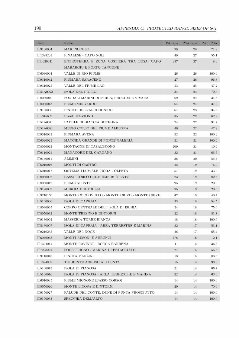
190 APPENDIX C. PROTECTED RANGE SIZES OF SCI
Code Name PA cells PSA cells Perc. PSA
IT9130004 MAR PICCOLO 39 28 71.8
IT1323201 FINALESE - CAPO NOLI 49 27 55.1
ITB020041 ENTROTERRA E ZONA COSTIERA TRA BOSA, CAPO
MARARGIU E PORTO TANGONE
337 27 8.0
IT6030004 VALLE DI RIO FIUME 26 26 100.0
IT9310042 FIUMARA SARACENO 27 26 96.3
IT9310025 VALLE DEL FIUME LAO 53 25 47.2
IT51A0023 ISOLA DEL GIGLIO 34 24 70.6
IT8030010 FONDALI MARINI DI ISCHIA, PROCIDA E VIVARA 69 24 34.8
IT8050013 FIUME MINGARDO 64 24 37.5
IT9130006 PINETE DELL’ARCO IONICO 67 23 34.3
IT1315602 PIZZO D’EVIGNO 35 22 62.9
IT51A0011 PADULE DI DIACCIA BOTRONA 24 22 91.7
IT51A0021 MEDIO CORSO DEL FIUME ALBEGNA 46 22 47.8
IT9310043 FIUMARA AVENA 22 22 100.0
IT6030025 MACCHIA GRANDE DI PONTE GALERIA 21 21 100.0
IT8050022 MONTAGNE DI CASALBUONO 209 21 10.0
IT9110025 MANACORE DEL GARGANO 32 21 65.6
IT9150011 ALIMINI 36 20 55.6
IT6010016 MONTI DI CASTRO 25 19 76.0
IT6010017 SISTEMA FLUVIALE FIORA - OLPETA 57 19 33.3
IT8050007 BASSO CORSO DEL FIUME BUSSENTO 23 19 82.6
IT8050012 FIUME ALENTO 95 19 20.0
IT9120002 MURGIA DEI TRULLI 95 19 20.0
IT9210150 MONTE COCCOVELLO - MONTE CRIVO - MONTE CRIVE 47 19 40.4
IT5160006 ISOLA DI CAPRAIA 33 18 54.5
IT8030005 CORPO CENTRALE DELL’ISOLA DI ISCHIA 24 18 75.0
IT8050032 MONTE TRESINO E DINTORNI 22 18 81.8
IT9130002 MASSERIA TORRE BIANCA 18 18 100.0
IT5160007 ISOLA DI CAPRAIA - AREA TERRESTRE E MARINA 32 17 53.1
IT9210265 VALLE DEL NOCE 26 17 65.4
IT6040043 MONTI AUSONI E AURUNCI 776 16 2.1
IT1324011 MONTE RAVINET - ROCCA BARBENA 41 15 36.6
IT7228221 FOCE TRIGNO - MARINA DI PETACCIATO 27 15 55.6
IT9110016 PINETA MARZINI 18 15 83.3
IT1324909 TORRENTE ARROSCIA E CENTA 15 14 93.3
IT5160013 ISOLA DI PIANOSA 21 14 66.7
IT5160016 ISOLA DI PIANOSA - AREA TERRESTRE E MARINA 22 14 63.6
IT6010035 FIUME MIGNONE (BASSO CORSO) 14 14 100.0
IT8050026 MONTE LICOSA E DINTORNI 20 14 70.0
IT9150027 PALUDE DEL CONTE, DUNE DI PUNTA PROSCIUTTO 14 14 100.0
IT9150033 SPECCHIA DELL’ALTO 14 14 100.0

191
Code Name PA cells PSA cells Perc. PSA
IT9220055 BOSCO PANTANO DI POLICORO E COSTA IONICA FOCE
SINNI
23 14 60.9
IT1315805 BASSA VALLE ARMEA 16 13 81.2
IT6030003 BOSCHI MESOFILI DI ALLUMIERE 13 13 100.0
IT6030047 BOSCO DI FOGLINO 13 13 100.0
IT6040010 LAGO DI FONDI 19 13 68.4
IT8030018 LAGO DI PATRIA 14 13 92.9
IT8050010 FASCE LITORANEE A DESTRA E A SINISTRA DEL FIUME
SELE
24 13 54.2
IT8050023 MONTE BULGHERIA 35 13 37.1
IT5160014 ISOLA DI MONTECRISTO 20 12 60.0
IT5160017 ISOLA DI MONTECRISTO E FORMICA DI MONTECRISTO
- AREA TERRESTRE E MARINA
20 12 60.0
IT6030044 MACCHIA DELLA SPADELLATA E FOSSO S. ANASTASIO 12 12 100.0
IT7222217 FOCE SACCIONE - BONIFICA RAMITELLI 20 12 60.0
IT9130001 TORRE COLIMENA 31 12 38.7
IT5160008 MONTE CALVI DI CAMPIGLIA 21 11 52.4
IT5160009 PROMONTORIO DI PIOMBINO E MONTE MASSONCELLO 16 11 68.8
IT51A0005 LAGO DELL’ACCESA 20 11 55.0
IT6030053 SUGHERETA DI CASTEL DI DECIMA 11 11 100.0
IT9150015 LITORALE DI GALLIPOLI E ISOLA S. ANDREA 18 11 61.1
IT9150030 BOSCO LA LIZZA E MACCHIA DEL PAGLIARONE 11 11 100.0
IT5160003 TOMBOLO DI CECINA 19 10 52.6
IT5160004 PADULE DI BOLGHERI 10 10 100.0
IT51A0010 POGGIO DI MOSCONA 15 10 66.7
IT51A0014 PINETA GRANDUCALE DELL’UCCELLINA 13 10 76.9
IT8050036 PARCO MARINO DI S. MARIA DI CASTELLABATE 21 10 47.6
IT9140002 LITORALE BRINDISINO 18 10 55.6
IT9150009 LITORALE DI UGENTO 27 10 37.0
IT1315720 FIUME ROIA 10 9 90.0
IT1324007 MONTE CIAZZE SECCHE 9 9 100.0
IT6030028 CASTEL PORZIANO (QUERCETI IGROFILI) 9 9 100.0
IT6040017 PROMONTORIO DEL CIRCEO (QUARTO FREDDO) 14 9 64.3
IT8030011 FONDALI MARINI DI PUNTA CAMPANELLA E CAPRI 69 9 13.0
IT8050011 FASCIA INTERNA DI COSTA DEGLI INFRESCHI E DELLA
MASSETA
23 9 39.1
IT9110002 VALLE FORTORE, LAGO DI OCCHITO 178 9 5.1
IT9150032 LE CESINE 19 9 47.4
IT9210155 MARINA DI CASTROCUCCO 13 9 69.2
ITB023037 COSTA E ENTROTERRA DI BOSA, SUNI E MONTRESTA 126 9 7.1
IT1315716 ROVERINO 9 8 88.9
IT51A0004 POGGIO TRE CANCELLI 8 8 100.0
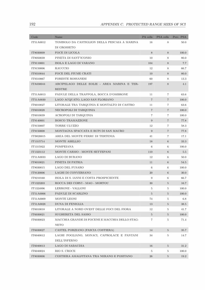
192 APPENDIX C. PROTECTED RANGE SIZES OF SCI
Code Name PA cells PSA cells Perc. PSA
IT51A0012 TOMBOLO DA CASTIGLION DELLA PESCAIA A MARINA
DI GROSSETO
16 8 50.0
IT8030009 FOCE DI LICOLA 8 8 100.0
IT8050039 PINETA DI SANT’ICONIO 10 8 80.0
IT9110001 ISOLA E LAGO DI VARANO 104 8 7.7
IT9150006 RAUCCIO 12 8 66.7
IT9310044 FOCE DEL FIUME CRATI 10 8 80.0
IT9310067 FORESTE ROSSANESI 60 8 13.3
ITA030044 ARCIPELAGO DELLE EOLIE - AREA MARINA E TER-
RESTRE
197 8 4.1
IT51A0013 PADULE DELLA TRAPPOLA, BOCCA D’OMBRONE 11 7 63.6
IT51A0030 LAGO ACQUATO, LAGO SAN FLORIANO 7 7 100.0
IT6010027 LITORALE TRA TARQUINIA E MONTALTO DI CASTRO 11 7 63.6
IT6010028 NECROPOLI DI TARQUINIA 7 7 100.0
IT6010039 ACROPOLI DI TARQUINIA 7 7 100.0
IT9140001 BOSCO TRAMAZZONE 9 7 77.8
IT9150007 TORRE ULUZZO 12 7 58.3
IT9150008 MONTAGNA SPACCATA E RUPI DI SAN MAURO 9 7 77.8
ITB020015 AREA DEL MONTE FERRU DI TERTENIA 41 7 17.1
IT1315714 MONTE ABELLIO 18 6 33.3
IT1315922 POMPEIANA 6 6 100.0
IT1323112 MONTE CARMO - MONTE SETTEPANI 110 6 5.5
IT51A0033 LAGO DI BURANO 12 6 50.0
IT8010021 PINETA DI PATRIA 11 6 54.5
IT8030015 LAGO DEL FUSARO 6 6 100.0
IT9120006 LAGHI DI CONVERSANO 20 6 30.0
IT9210160 ISOLA DI S. IANNI E COSTA PROSPICIENTE 9 6 66.7
IT1323203 ROCCA DEI CORVI - MAO - MORTOU 30 5 16.7
IT1324896 LERRONE - VALLONI 5 5 100.0
IT51A0006 PADULE DI SCARLINO 5 5 100.0
IT51A0009 MONTE LEONI 74 5 6.8
IT51A0028 DUNA DI FENIGLIA 13 5 38.5
IT6010018 LITORALE A NORD OVEST DELLE FOCI DEL FIORA 12 5 41.7
IT6030021 SUGHERETA DEL SASSO 5 5 100.0
IT6030023 MACCHIA GRANDE DI FOCENE E MACCHIA DELLO STAG-
NETO
7 5 71.4
IT6030027 CASTEL PORZIANO (FASCIA COSTIERA) 14 5 35.7
IT6040012 LAGHI FOGLIANO, MONACI, CAPROLACE E PANTANI
DELL’INFERNO
34 5 14.7
IT6040013 LAGO DI SABAUDIA 16 5 31.2
IT6040024 RIO S. CROCE 5 5 100.0
IT8030006 COSTIERA AMALFITANA TRA NERANO E POSITANO 26 5 19.2

193
Code Name PA cells PSA cells Perc. PSA
IT8030038 CORPO CENTRALE E RUPI COSTIERE OCCIDENTALI
DELL’ISOLA DI CAPRI
13 5 38.5
IT9140005 TORRE GUACETO E MACCHIA S. GIOVANNI 11 5 45.5
IT9150014 LE CESINE 14 5 35.7
IT9150031 MASSERIA ZANZARA 5 5 100.0
IT9210015 ACQUAFREDDA DI MARATEA 11 5 45.5
IT9310023 VALLE DEL FIUME ARGENTINO 68 5 7.4
IT9310052 CASONI DI SIBARI 9 5 55.6
IT1315719 TORRENTE NERVIA 5 4 80.0
IT5160010 PADULE ORTI - BOTTAGONE 4 4 100.0
IT6030006 MONTE TOSTO 4 4 100.0
IT6030026 LAGO DI TRAIANO 4 4 100.0
IT6040016 PROMONTORIO DEL CIRCEO (QUARTO CALDO) 12 4 33.3
IT6040018 DUNE DEL CIRCEO 33 4 12.1
IT8010020 PINETA DI CASTELVOLTURNO 4 4 100.0
IT8010027 FIUMI VOLTURNO E CALORE BENEVENTANO 219 4 1.8
IT8010028 FOCE VOLTURNO - VARICONI 8 4 50.0
IT8050038 PARETI ROCCIOSE DI CALA DEL CEFALO 6 4 66.7
IT9140006 BOSCO DI SANTA TERESA 4 4 100.0
IT9140009 FOCE CANALE GIANCOLA 5 4 80.0
IT9150021 BOSCO LE CHIUSE 4 4 100.0
IT9150029 BOSCO DI CERVALORA 4 4 100.0
IT9220080 COSTA IONICA FOCE AGRI 17 4 23.5
IT9220085 COSTA IONICA FOCE BASENTO 13 4 30.8
IT9220090 COSTA IONICA FOCE BRADANO 14 4 28.6
IT9350300 COSTA VIOLA 239 4 1.7
ITA030010 FIUME FIUMEDINISI, MONTE SCUDERI 89 4 4.5
ITA030029 ISOLA DI SALINA (STAGNO DI LINGUA) 20 4 20.0
ITA030043 MONTI NEBRODI 819 4 0.5
IT51A0015 DUNE COSTIERE DEL PARCO DELL’UCCELLINA 10 3 30.0
IT51A0024 ISOLA DI GIANNUTRI 10 3 30.0
IT51A0031 LAGO DI BURANO 7 3 42.9
IT51A0037 ISOLA DI GIANNUTRI - AREA TERRESTRE E MARINA 10 3 30.0
IT6010019 PIAN DEI CANGANI 4 3 75.0
IT6010026 SALINE DI TARQUINIA 6 3 50.0
IT6030016 ANTICA LAVINIUM - PRATICA DI MARE 3 3 100.0
IT6030019 MACCHIATONDA 6 3 50.0
IT6030045 LIDO DEI GIGLI 6 3 50.0
IT7222216 FOCE BIFERNO - LITORALE DI CAMPOMARINO 19 3 15.8
IT7228230 LAGO DI GUARDIALFIERA - FOCE FIUME BIFERNO 401 3 0.7
IT8010019 PINETA DELLA FOCE DEL GARIGLIANO 7 3 42.9
IT8030019 MONTE BARBARO E CRATERE DI CAMPIGLIONE 10 3 30.0
IT8030026 RUPI COSTIERE DELL’ISOLA DI ISCHIA 22 3 13.6

194 APPENDIX C. PROTECTED RANGE SIZES OF SCI
Code Name PA cells PSA cells Perc. PSA
IT8050024 MONTE CERVATI, CENTAURINO E MONTAGNE DI LAU-
RINO
330 3 0.9
IT8050040 RUPI COSTIERE DELLA COSTA DEGLI INFRESCHI E
DELLA MASSETA
15 3 20.0
IT9140003 STAGNI E SALINE DI PUNTA DELLA CONTESSA 10 3 30.0
IT9140007 BOSCO CURTIPETRIZZI 3 3 100.0
IT9140008 TORRE GUACETO 8 3 37.5
IT9150013 PALUDE DEL CAPITANO 4 3 75.0
IT9150018 BOSCO SERRA DEI CIANCI 5 3 60.0
IT9150024 TORRE INSERRAGLIO 5 3 60.0
IT9150025 TORRE VENERI 12 3 25.0
IT1325624 CAPO MELE 7 2 28.6
IT5160002 ISOLA DI GORGONA 6 2 33.3
IT5160005 BOSCHI DI BOLGHERI, BIBBONA E CASTIGLIONCELLO 54 2 3.7
IT5160015 ISOLA DI GORGONA - AREA TERRESTRE E MARINA 7 2 28.6
IT51A0007 PUNTA ALA E ISOLOTTO DELLO SPARVIERO 11 2 18.2
IT51A0032 DUNA DEL LAGO DI BURANO 7 2 28.6
IT6010040 MONTEROZZI 2 2 100.0
IT6030001 FIUME MIGNONE (MEDIO CORSO) 25 2 8.0
IT6030020 TORRE FLAVIA 3 2 66.7
IT6030046 TOR CALDARA (ZONA SOLFATARE E FOSSI) 2 2 100.0
IT6030048 LITORALE DI TORRE ASTURA 15 2 13.3
IT6030049 ZONE UMIDE A OVEST DEL FIUME ASTURA 3 2 66.7
IT6040007 MONTE LEANO 12 2 16.7
IT6040011 LAGO LUNGO 4 2 50.0
IT6040022 COSTA ROCCIOSA TRA SPERLONGA E GAETA 19 2 10.5
IT6040025 FIUME GARIGLIANO (TRATTO TERMINALE) 4 2 50.0
IT7140109 MARINA DI VASTO 4 2 50.0
IT8010018 VARICONI 6 2 33.3
IT8010029 FIUME GARIGLIANO 46 2 4.3
IT8030013 ISOLOTTO DI S. MARTINO E DINTORNI 2 2 100.0
IT8030014 LAGO D’AVERNO 4 2 50.0
IT8030020 MONTE NUOVO 4 2 50.0
IT8030022 PINETE DELL’ISOLA DI ISCHIA 3 2 66.7
IT8030024 PUNTA CAMPANELLA 10 2 20.0
IT8030034 STAZIONE DI CYPERUS POLYSTACHYUS DI ISCHIA 2 2 100.0
IT8050037 PARCO MARINO DI PUNTA DEGLI INFRESCHI 24 2 8.3
IT8050041 SCOGLIO DEL MINGARDO E SPIAGGIA DI CALA DEL CE-
FALO
5 2 40.0
IT9110030 BOSCO QUARTO - MONTE SPIGNO 105 2 1.9
IT9140004 BOSCO I LUCCI 2 2 100.0
IT9150001 BOSCO GUARINI 2 2 100.0
IT9150003 AQUATINA DI FRIGOLE 7 2 28.6
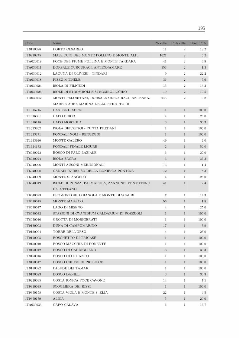
195
Code Name PA cells PSA cells Perc. PSA
IT9150028 PORTO CESAREO 11 2 18.2
IT9210275 MASSICCIO DEL MONTE POLLINO E MONTE ALPI 1021 2 0.2
ITA020018 FOCE DEL FIUME POLLINA E MONTE TARDARA 41 2 4.9
ITA030011 DORSALE CURCURACI, ANTENNAMARE 153 2 1.3
ITA030012 LAGUNA DI OLIVERI - TINDARI 9 2 22.2
ITA030018 PIZZO MICHELE 36 2 5.6
ITA030024 ISOLA DI FILICUDI 15 2 13.3
ITA030026 ISOLE DI STROMBOLI E STROMBOLICCHIO 19 2 10.5
ITA030042 MONTI PELORITANI, DORSALE CURCURACI, ANTENNA-
MARE E AREA MARINA DELLO STRETTO DI
245 2 0.8
IT1315715 CASTEL D’APPIO 1 1 100.0
IT1316001 CAPO BERTA 4 1 25.0
IT1316118 CAPO MORTOLA 3 1 33.3
IT1323202 ISOLA BERGEGGI - PUNTA PREDANI 1 1 100.0
IT1323271 FONDALI NOLI - BERGEGGI 1 1 100.0
IT1323920 MONTE GALERO 49 1 2.0
IT1324172 FONDALI FINALE LIGURE 2 1 50.0
IT6030022 BOSCO DI PALO LAZIALE 5 1 20.0
IT6030024 ISOLA SACRA 3 1 33.3
IT6040006 MONTI AUSONI MERIDIONALI 73 1 1.4
IT6040008 CANALI IN DISUSO DELLA BONIFICA PONTINA 12 1 8.3
IT6040009 MONTE S. ANGELO 4 1 25.0
IT6040019 ISOLE DI PONZA, PALMAROLA, ZANNONE, VENTOTENE
E S. STEFANO
41 1 2.4
IT6040023 PROMONTORIO GIANOLA E MONTE DI SCAURI 7 1 14.3
IT8010015 MONTE MASSICO 56 1 1.8
IT8030017 LAGO DI MISENO 4 1 25.0
IT8030032 STAZIONI DI CYANIDIUM CALDARIUM DI POZZUOLI 1 1 100.0
IT8050016 GROTTA DI MORIGERATI 1 1 100.0
IT9130003 DUNA DI CAMPOMARINO 17 1 5.9
IT9150004 TORRE DELL’ORSO 4 1 25.0
IT9150005 BOSCHETTO DI TRICASE 1 1 100.0
IT9150010 BOSCO MACCHIA DI PONENTE 1 1 100.0
IT9150012 BOSCO DI CARDIGLIANO 3 1 33.3
IT9150016 BOSCO DI OTRANTO 1 1 100.0
IT9150017 BOSCO CHIUSO DI PRESICCE 1 1 100.0
IT9150022 PALUDE DEI TAMARI 1 1 100.0
IT9150023 BOSCO DANIELI 3 1 33.3
IT9220095 COSTA IONICA FOCE CAVONE 14 1 7.1
IT9310038 SCOGLIERA DEI RIZZI 1 1 100.0
IT9350158 COSTA VIOLA E MONTE S. ELIA 22 1 4.5
IT9350179 ALICA 5 1 20.0
ITA030033 CAPO CALAVA 6 1 16.7

196 APPENDIX C. PROTECTED RANGE SIZES OF SCI
Code Name PA cells PSA cells Perc. PSA
ITB010001 ISOLA ASINARA 86 1 1.2
ITB010082 ISOLA DELL’ASINARA 91 1 1.1
ITB020012 BERCHIDA E BIDDEROSA 37 1 2.7
ITALY TOTAL: 16585 4774 28.8
PORTUGAL
PTZPE0004 RIA DE AVEIRO 425 39 9.2
PORTUGAL TOTAL: 425 39 9.2
OVERALL NATURA 2000 TOTAL: 59158 28327 47.9

197
Table C.2: Asplenium majoricum EOO and AOO protection by Natura 2000 protected
areas
Code Name PA cells EOO cells Perc. EOO AOO cells Perc. AOO
SPAIN
ES0000453MUNTANYES DE LA MARINA 557 500 89.8 499 89.6
ES0000474SERRES DE MARIOLA I EL CARRASCAL DE
LA FONT ROJA
278 273 98.2 264 95.0
ES0000023L’ALBUFERA 255 255 100.0 255 100.0
ES0000471L’ALBUFERA 255 255 100.0 255 100.0
ES0000213SERRES DE MARIOLA I EL CARRASCAR DE
LA FONT ROJA
246 244 99.2 235 95.5
ES5213042VALLS DE LA MARINA 212 212 100.0 212 100.0
ES5213019AITANA, SERRELLA I PUIGCAMPANA 239 209 87.4 208 87.0
ES0000451MONTDUVER-MARJAL DE LA SAFOR 149 149 100.0 149 100.0
ES5233015SERRES DEL MONTDUVER I MARXUQUERA 122 122 100.0 122 100.0
ES0000444SERRA D’IRTA 105 105 100.0 94 89.5
ES5223036SERRA D’IRTA 105 105 100.0 94 89.5
ES5233013SERRA DE CORBERA 83 83 100.0 83 100.0
ES5310027CIMALS DE LA SERRA 135 80 59.3 80 59.3
ES5140005SERRA DE MONTSIA 83 67 80.7 66 79.5
ES0000441D’ALFABIA A BINIARROI 112 64 57.1 64 57.1
ES0000468SERRA D’ESPADA 751 56 7.5 56 7.5
ES5233041SERRA DE LA SAFOR 49 49 100.0 49 100.0
ES0000446DESERT DE LES PALMES 48 48 100.0 48 100.0
ES5221002DESERT DE LES PALMES 47 47 100.0 47 100.0
ES5232007RIU XUQUER 74 65 87.8 47 63.5
ES0000463CABECO D’OR I LA GRANA 74 45 60.8 45 60.8
ES0000445PLANIOLS-BENASQUES 38 38 100.0 38 100.0
ES0000454MONTGO-CAP DE SANT ANTONI 40 40 100.0 37 92.5
ES5211007MONTGO 40 40 100.0 37 92.5
ES5310008ES GALATZO-S’ESCLOP 36 36 100.0 36 100.0
ES0000212SIERRA DE MARTES-MUELA DE CORTES 1554 40 2.6 35 2.3
ES0000450MARJAL I ESTANYS D’ALMENARA 32 32 100.0 32 100.0
ES5223007MARJAL D’ALMENARA 32 32 100.0 32 100.0
ES5213020SERRES DEL FERRER I BERNIA 57 30 52.6 30 52.6
ES0000440DES TEIX AL PUIG DE SES FITES 32 28 87.5 28 87.5
ES5212004RIU GORGOS 27 27 100.0 27 100.0
ES5232008CURS MITJA DEL RIU ALBAIDA 27 27 100.0 27 100.0
ES0000469SERRA CALDERONA 253 25 9.9 25 9.9
ES5140002SERRA DE GODALL 34 25 73.5 25 73.5
ES5232002SERRA CALDERONA 240 25 10.4 25 10.4
ES0000147MARJAL DE PEGO-OLIVA. 24 24 100.0 24 100.0
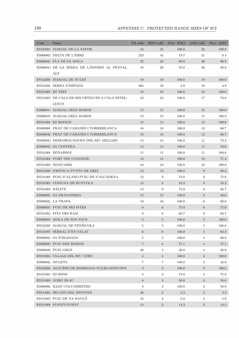
198 APPENDIX C. PROTECTED RANGE SIZES OF SCI
Code Name PA cells EOO cells Perc. EOO AOO cells Perc. AOO
ES5233030MARJAL DE LA SAFOR 24 24 100.0 24 100.0
ES0000020DELTA DE L’EBRE 223 44 19.7 21 9.4
ES0000439PLA DE SA MOLA 22 20 90.9 20 90.9
ES0000442DE LA SERRA DE L’ESPERO AL PENYAL
ALT
34 20 58.8 20 58.8
ES5222005MARJAL DE NULES 19 19 100.0 19 100.0
ES5222001SERRA D’ESPADA 364 18 4.9 18 4.9
ES5310009ES TEIX 18 18 100.0 18 100.0
ES5310078DE CALA DE SES ORTIGUES A CALA ESTEL-
LENCS
23 23 100.0 17 73.9
ES0000148MARJAL DELS MOROS. 15 15 100.0 15 100.0
ES0000470MARJAL DELS MOROS 15 15 100.0 15 100.0
ES5310083ES BOIXOS 15 15 100.0 15 100.0
ES0000060PRAT DE CABANES I TORREBLANCA. 18 18 100.0 12 66.7
ES0000467PRAT DE CABANES I TORREBLANCA 18 18 100.0 12 66.7
ES0000211DESEMBOCADURA DEL RIU MILLARS 15 15 100.0 11 73.3
ES0000225SA COSTERA 14 14 100.0 11 78.6
ES5310089BINIARROI 11 11 100.0 11 100.0
ES5310081PORT DES CANONGE 14 14 100.0 10 71.4
ES5310085MONCAIRE 10 10 100.0 10 100.0
ES5310082S’ESTACA-PUNTA DE DEIA 13 13 100.0 9 69.2
ES5310090PUIG D’ALARO-PUIG DE S’ALCADENA 12 9 75.0 9 75.0
ES5310010COMUNA DE BUNYOLA 15 8 53.3 8 53.3
ES5310087BALITX 12 9 75.0 8 66.7
ES0000221SA DRAGONERA 15 15 100.0 6 40.0
ES0000222LA TRAPA 10 10 100.0 6 60.0
ES0000379PUIG DE SES FITES 8 6 75.0 6 75.0
ES5310026FITA DES RAM 9 6 66.7 6 66.7
ES0000377MOLA DE SON PACS 5 5 100.0 5 100.0
ES5222002MARJAL DE PENISCOLA 5 5 100.0 5 100.0
ES5310076SERRAL D’EN SALAT 6 6 100.0 5 83.3
ES0000223SA FORADADA 5 5 100.0 4 80.0
ES0000378PUIG DES BOIXOS 7 4 57.1 4 57.1
ES0000381PUIG GROS 20 4 20.0 4 20.0
ES5233047ULLALS DEL RIU VERD 4 4 100.0 4 100.0
ES0000224MULETA 7 7 100.0 3 42.9
ES5222007ALGUERS DE BORRIANA-NULES-MONCOFA 3 3 100.0 3 100.0
ES5310028ES BINIS 4 3 75.0 3 75.0
ES5310088GORG BLAU 6 3 50.0 3 50.0
ES0000061ILLES COLUMBRETES 4 4 100.0 2 50.0
ES5140023SECANS DEL MONTSIA 46 2 4.3 2 4.3
ES5310079PUIG DE NA BAUCA 34 2 5.9 2 5.9
ES5310080PUIGPUNYENT 14 2 14.3 2 14.3
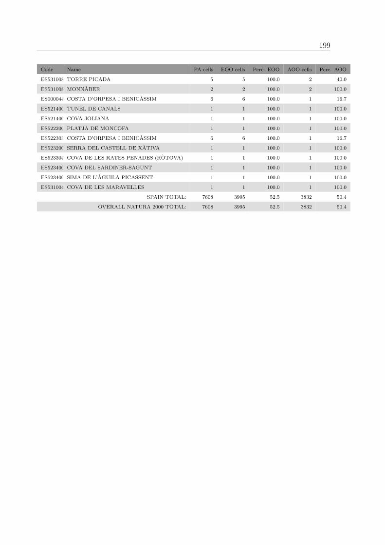
199
Code Name PA cells EOO cells Perc. EOO AOO cells Perc. AOO
ES5310084TORRE PICADA 5 5 100.0 2 40.0
ES5310086MONNABER 2 2 100.0 2 100.0
ES0000447COSTA D’ORPESA I BENICASSIM 6 6 100.0 1 16.7
ES5214002TUNEL DE CANALS 1 1 100.0 1 100.0
ES5214004COVA JOLIANA 1 1 100.0 1 100.0
ES5222006PLATJA DE MONCOFA 1 1 100.0 1 100.0
ES5223037COSTA D’ORPESA I BENICASSIM 6 6 100.0 1 16.7
ES5232009SERRA DEL CASTELL DE XATIVA 1 1 100.0 1 100.0
ES5233049COVA DE LES RATES PENADES (ROTOVA) 1 1 100.0 1 100.0
ES5234001COVA DEL SARDINER-SAGUNT 1 1 100.0 1 100.0
ES5234005SIMA DE L’AGUILA-PICASSENT 1 1 100.0 1 100.0
ES5310040COVA DE LES MARAVELLES 1 1 100.0 1 100.0
SPAIN TOTAL: 7608 3995 52.5 3832 50.4
OVERALL NATURA 2000 TOTAL: 7608 3995 52.5 3832 50.4
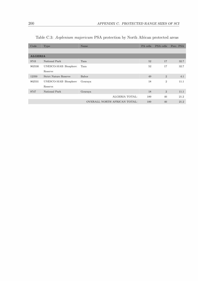
200 APPENDIX C. PROTECTED RANGE SIZES OF SCI
Table C.3: Asplenium majoricum PSA protection by North African protected areas
Code Type Name PA cells PSA cells Perc. PSA
ALGERIA
9743 National Park Taza 52 17 32.7
902530 UNESCO-MAB Biosphere
Reserve
Taza 52 17 32.7
12350 Strict Nature Reserve Babor 49 2 4.1
902531 UNESCO-MAB Biosphere
Reserve
Gouraya 18 2 11.1
9747 National Park Gouraya 18 2 11.1
ALGERIA TOTAL: 189 40 21.2
OVERALL NORTH AFRICAN TOTAL: 189 40 21.2

201
Carduncellus dianius
Table C.4: Carduncellus dianius PSA protection by Natura 2000 protected areas
Code Name PA cells PSA cells Perc. PSA
SPAIN
ES0000023 L’ALBUFERA 255 185 72.5
ES0000471 L’ALBUFERA 255 185 72.5
ES0000020 DELTA DE L’EBRE 223 145 65.0
ES0000453 MUNTANYES DE LA MARINA 557 112 20.1
ES0000227 MUNTANYES D’ARTA 129 105 81.4
ES0000073 COSTA BRAVA DE MALLORCA 143 101 70.6
ES0000451 MONTDUVER-MARJAL DE LA SAFOR 149 82 55.0
ES0000230 LA VALL 74 70 94.6
ES0000081 CAP ENDERROCAT-CAP BLANC 80 64 80.0
ES5233015 SERRES DEL MONTDUVER I MARXUQUERA 122 59 48.4
ES0000228 CAP DE SES SALINES 60 51 85.0
ES0000231 DELS ALOCS A FORNELLS 52 49 94.2
ES5213020 SERRES DEL FERRER I BERNIA 57 49 86.0
ES0000084 SES SALINES D’EIVISSA I FORMENTERA 76 47 61.8
ES5310032 CAP LLENTRISCA-SA TALAIA 50 46 92.0
ES0000444 SERRA D’IRTA 105 44 41.9
ES5223036 SERRA D’IRTA 105 44 41.9
ES5310113 LA VALL 46 44 95.7
ES0000083 ARXIPELAG DE CABRERA 75 42 56.0
ES0000237 DES CANUTELLS A LLUCALARI 45 40 88.9
ES5213042 VALLS DE LA MARINA 212 40 18.9
ES0000454 MONTGO-CAP DE SANT ANTONI 40 37 92.5
ES5211007 MONTGO 40 37 92.5
ES0000038 S’ALBUFERA DE MALLORCA 39 36 92.3
ES0000443 SUD DE CIUTADELLA 38 35 92.1
ES5233013 SERRA DE CORBERA 83 34 41.0
ES0000239 DE BINIGAUS A CALA MITJANA 48 33 68.8
ES5310105 ES AMUNTS D’EIVISSA 36 33 91.7
ES0000450 MARJAL I ESTANYS D’ALMENARA 32 32 100.0
ES5223007 MARJAL D’ALMENARA 32 32 100.0
ES0000235 DE S’ALBUFERA A LA MOLA 41 31 75.6
ES5310029 NA BORGES 69 28 40.6
ES5310035 AREA MARINA DEL NORD DE MENORCA 34 28 82.4
ES0000238 SON BOU I BARRANC DE SA VALL 29 27 93.1
ES5140005 SERRA DE MONTSIA 83 27 32.5

202 APPENDIX C. PROTECTED RANGE SIZES OF SCI
Code Name PA cells PSA cells Perc. PSA
ES0000234 S’ALBUFERA DES GRAU 31 26 83.9
ES5310008 ES GALATZO-S’ESCLOP 36 25 69.4
ES5310034 SERRA GROSSA 25 25 100.0
ES5310112 NORD DE SANT JOAN 26 25 96.2
ES0000147 MARJAL DE PEGO-OLIVA. 24 24 100.0
ES5233030 MARJAL DE LA SAFOR 24 24 100.0
ES5213018 PENYA-SEGATS DE LA MARINA 31 23 74.2
ES5213019 AITANA, SERRELLA I PUIGCAMPANA 239 23 9.6
ES0000037 ES TRENC-SALOBRAR DE CAMPOS 26 22 84.6
ES0000232 LA MOLA I S’ALBUFERA DE FORNELLS 29 22 75.9
ES0000233 D’ADDAIA A S’ALBUFERA 35 22 62.9
ES0000241 COSTA DELS AMUNTS 21 20 95.2
ES5310005 BADIES DE POLLENCA I ALCUDIA 50 20 40.0
ES5222005 MARJAL DE NULES 19 19 100.0
ES0000121 ILLOTS DE BENIDORM I SERRA GELADA 27 18 66.7
ES0000439 PLA DE SA MOLA 22 18 81.8
ES5140009 TIVISSA-VANDELLOS-LLABERIA 321 17 5.3
ES5310024 LA MOLA 27 17 63.0
ES5310078 DE CALA DE SES ORTIGUES A CALA ESTELLENCS 23 17 73.9
ES5213021 SERRA GELADA I LITORAL DE LA MARINA BAIXA 25 16 64.0
ES5310033 XARRACA 19 16 84.2
ES0000148 MARJAL DELS MOROS. 15 15 100.0
ES0000470 MARJAL DELS MOROS 15 15 100.0
ES0000074 CAP DE CALA FIGUERA 20 14 70.0
ES0000120 SALINAS DE SANTA POLA. 44 14 31.8
ES0000145 MONDRAGO 15 14 93.3
ES0000229 COSTA NORD DE CIUTADELLA 17 14 82.4
ES0000240 COSTA SUD DE CIUTADELLA 25 14 56.0
ES5232007 RIU XUQUER 74 14 18.9
ES0000386 CAPELL DE FERRO 30 13 43.3
ES0000463 CABECO D’OR I LA GRANA 74 13 17.6
ES5310079 PUIG DE NA BAUCA 34 13 38.2
ES0000060 PRAT DE CABANES I TORREBLANCA. 18 12 66.7
ES0000459 IFAC I LITORAL DE LA MARINA 14 12 85.7
ES0000467 PRAT DE CABANES I TORREBLANCA 18 12 66.7
ES5211009 IFAC 14 12 85.7
ES5310030 COSTA DE LLEVANT 28 12 42.9
ES5310098 CALES DE MANACOR 16 12 75.0
ES0000079 LA VICTORIA 16 11 68.8
ES5310104 COSTA DE L’OEST D’EIVISSA 26 11 42.3
ES0000225 SA COSTERA 14 10 71.4
ES5310023 ILLOTS DE PONENT D’EIVISSA 13 10 76.9
ES5310025 CAP DE BARBARIA 18 10 55.6

203
Code Name PA cells PSA cells Perc. PSA
ES5310081 PORT DES CANONGE 14 10 71.4
ES0000226 L’ALBUFERETA 10 9 90.0
ES5140001 LITORAL MERIDIONAL TARRAGONI 20 9 45.0
ES5310068 CAP NEGRE 9 9 100.0
ES5310082 S’ESTACA-PUNTA DE DEIA 13 9 69.2
ES5310087 BALITX 12 9 75.0
ES5310111 AREA MARINA PLATJA DE MIGJORN 22 9 40.9
ES0000446 DESERT DE LES PALMES 48 8 16.7
ES5213024 TABARCA 24 8 33.3
ES5221002 DESERT DE LES PALMES 47 8 17.0
ES0000175 SALINAS Y ARENALES DE SAN PEDRO DEL PINATAR 17 7 41.2
ES5212009 ALGEPSARS DE FINESTRAT 7 7 100.0
ES5310074 DE CALA LLUCALARI A CALES COVES 12 7 58.3
ES5310083 ES BOIXOS 15 7 46.7
ES5310092 MUNTANYES DE POLLENCA 54 7 13.0
ES0000221 SA DRAGONERA 15 6 40.0
ES0000222 LA TRAPA 10 6 60.0
ES0000260 MAR MENOR 67 6 9.0
ES0000385 BARBATX 24 6 25.0
ES0000462 CLOT DE GALVANY 12 6 50.0
ES5140022 BARRANC DE SANTES CREUS 9 6 66.7
ES5213025 DUNES DE GUARDAMAR 19 6 31.6
ES5213033 CABO ROIG 11 6 54.5
ES5310015 PUIG DE SANT MARTI 6 6 100.0
ES5310093 FORMENTOR 7 6 85.7
ES0000211 DESEMBOCADURA DEL RIU MILLARS 15 5 33.3
ES0000377 MOLA DE SON PACS 5 5 100.0
ES0000440 DES TEIX AL PUIG DE SES FITES 32 5 15.6
ES5213032 CAP DE LES HORTES 15 5 33.3
ES5222002 MARJAL DE PENISCOLA 5 5 100.0
ES5310076 SERRAL D’EN SALAT 6 5 83.3
ES5310107 AREA MARINA DE TAGOMAGO 6 5 83.3
ES0000078 ES VEDRA-ES VEDRANELL 6 4 66.7
ES0000223 SA FORADADA 5 4 80.0
ES0000384 BARRANC DE SANTA ANNA 4 4 100.0
ES5310036 AREA MARINA DEL SUD DE CIUTADELLA 20 4 20.0
ES5310070 PUNTA REDONA-ARENAL D’EN CASTELL 10 4 40.0
ES5310085 MONCAIRE 10 4 40.0
ES5310096 PUNTA DE N’AMER 6 4 66.7
ES6200030 MAR MENOR 45 4 8.9
ES0000080 CAP VERMELL 6 3 50.0
ES0000082 TAGOMAGO 3 3 100.0
ES0000224 MULETA 7 3 42.9

204 APPENDIX C. PROTECTED RANGE SIZES OF SCI
Code Name PA cells PSA cells Perc. PSA
ES0000378 PUIG DES BOIXOS 7 3 42.9
ES5222007 ALGUERS DE BORRIANA-NULES-MONCOFA 3 3 100.0
ES5310027 CIMALS DE LA SERRA 135 3 2.2
ES5310028 ES BINIS 4 3 75.0
ES5310031 PORROIG 3 3 100.0
ES5310037 BASSES DE LA MARINA DE LLUCMAJOR 3 3 100.0
ES5310099 PORTOCOLOM 5 3 60.0
ES5310109 AREA MARINA DE CALA SAONA 4 3 75.0
ES5310120 ES CLOT DES GUIX 3 3 100.0
ES0000061 ILLES COLUMBRETES 4 2 50.0
ES0000214 ILLOTS DE TABARCA 12 2 16.7
ES5212004 RIU GORGOS 27 2 7.4
ES5212012 SIERRA DE ESCALONA Y DEHESA DE CAMPOAMOR 77 2 2.6
ES5310009 ES TEIX 18 2 11.1
ES5310026 FITA DES RAM 9 2 22.2
ES5310069 CALA D’ALGAIRENS 3 2 66.7
ES5310084 TORRE PICADA 5 2 40.0
ES5310091 MOSSA 11 2 18.2
ES5310106 AREA MARINA DE SES MARGALIDES 2 2 100.0
ES5310108 AREA MARINA DEL CAP MARTINET 7 2 28.6
ES5310114 BINIGAFULL 2 2 100.0
ES5310115 ES MOLINET 2 2 100.0
ES5310118 TORRE LLAFUDA 4 2 50.0
ES5310119 PENYES D’EGIPTE 3 2 66.7
ES6200006 ESPACIOS ABIERTOS E ISLAS DEL MAR MENOR 40 2 5.0
ES6200029 FRANJA LITORAL SUMERGIDA DE LA REGION DE MUR-
CIA
70 2 2.9
ES0000059 LLACUNES DE LA MATA I TORREVIEJA. 60 1 1.7
ES0000447 COSTA D’ORPESA I BENICASSIM 6 1 16.7
ES5140004 SEQUIA MAJOR 4 1 25.0
ES5140016 TOSSAL DE MONTAGUT 28 1 3.6
ES5222006 PLATJA DE MONCOFA 1 1 100.0
ES5223037 COSTA D’ORPESA I BENICASSIM 6 1 16.7
ES5234001 COVA DEL SARDINER-SAGUNT 1 1 100.0
ES5310048 COVA DE SA GUITARRETA 1 1 100.0
ES5310050 COVA D’EN BESSO 1 1 100.0
ES5310055 COVA DES PIRATA 1 1 100.0
ES5310056 COVA DES PONT 1 1 100.0
ES5310057 COVA DE CAL PESSO 1 1 100.0
ES5310059 COVA DE LLENAIRE 1 1 100.0
ES5310072 CALETA DE BINILLAUTI 1 1 100.0
ES5310075 ARENAL DE SON SAURA 5 1 20.0
ES5310080 PUIGPUNYENT 14 1 7.1

205
Code Name PA cells PSA cells Perc. PSA
ES5310095 CAN PICAFORT 3 1 33.3
ES5310100 PUNTA DES RAS 2 1 50.0
ES5310123 BASSA DE FORMENTERA 1 1 100.0
SPAIN TOTAL: 6463 3109 48.1
FRANCE
FR9301592 CAMARGUE 884 104 11.8
FR9310019 CAMARGUE 899 104 11.6
FR9400574 PORTO/SCANDOLA/REVELLATA/CALVI/CALANCHES
DE PIANA (ZONE TERRESTRE ET MARINE)
202 101 50.0
FR9400570 AGRIATES 151 81 53.6
FR9410023 GOLFE DE PORTO ET PRESQU’ILE DE SCANDOLA 181 80 44.2
FR9101440 COMPLEXE LAGUNAIRE DE BAGES-SIGEAN 106 49 46.2
FR9112007 ETANGS DU NARBONNAIS 142 49 34.5
FR9301613 RADE D’HYERES 141 48 34.0
FR9101406 PETITE CAMARGUE 405 41 10.1
FR9310020 ILES D’HYERES 130 38 29.2
FR9301601 COTE BLEUE - CHAINE DE L’ESTAQUE 84 37 44.0
FR9112013 PETITE CAMARGUE LAGUNO-MARINE 208 35 16.8
FR9301622 LA PLAINE ET LE MASSIF DES MAURES 450 32 7.1
FR9402013 PLATEAU DU CAP CORSE 40 30 75.0
FR9101410 ETANGS PALAVASIENS 100 29 29.0
FR9110042 ETANGS PALAVASIENS ET ETANG DE L’ESTAGNOL 100 29 29.0
FR9400568 CAP CORSE NORD ET ILE FINOCCHIAROLA, GIRAGLIA
ET CAPENSE (COTE DE MACINAGGIO A C
47 26 55.3
FR9412009 PLATEAU DU CAP CORSE 32 26 81.2
FR9400571 ETANG DE BIGUGLIA 37 23 62.2
FR9410097 ILES FINOCCHIAROLA ET COTE NORD 27 22 81.5
FR9410101 ETANG DE BIGUGLIA 35 22 62.9
FR9101463 COMPLEXE LAGUNAIRE DE SALSES 89 21 23.6
FR9112005 COMPLEXE LAGUNAIRE DE SALSES-LEUCATE 85 21 24.7
FR9412010 CAPU ROSSU , SCANDOLA, REVELLATA, CALVI 40 21 52.5
FR9301590 LE RHONE AVAL 318 18 5.7
FR9301627 EMBOUCHURE DE L’ARGENS 24 17 70.8
FR9101411 HERBIERS DE L’ETANG DE THAU 67 16 23.9
FR9112018 ETANG DE THAU ET LIDO DE SETE A AGDE 110 16 14.5
FR9312008 SALINS D’HYERES ET DES PESQUIERS 21 16 76.2
FR9101408 ETANG DE MAUGUIO 102 15 14.7
FR9112017 ETANG DE MAUGUIO 102 15 14.7
FR9312015 ETANGS ENTRE ISTRES ET FOS 28 13 46.4
FR9402018 CAP ROSSU, SCANDOLA, POINTE DE LA REVELETTA,
CANYON DE CALVI
25 13 52.0
FR9301610 CAP SICIE - SIX FOURS 18 10 55.6
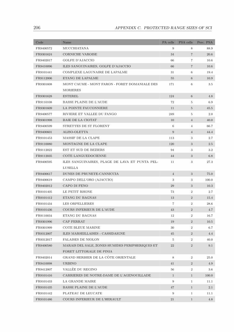
206 APPENDIX C. PROTECTED RANGE SIZES OF SCI
Code Name PA cells PSA cells Perc. PSA
FR9400572 MUCCHIATANA 9 8 88.9
FR9301624 CORNICHE VAROISE 34 7 20.6
FR9402017 GOLFE D’AJACCIO 66 7 10.6
FR9410096 ILES SANGUINAIRES, GOLFE D’AJACCIO 66 7 10.6
FR9101441 COMPLEXE LAGUNAIRE DE LAPALME 31 6 19.4
FR9112006 ETANG DE LAPALME 55 6 10.9
FR9301608 MONT CAUME - MONT FARON - FORET DOMANIALE DES
MORIERES
171 6 3.5
FR9301628 ESTEREL 124 6 4.8
FR9110108 BASSE PLAINE DE L’AUDE 72 5 6.9
FR9301609 LA POINTE FAUCONNIERE 11 5 45.5
FR9400577 RIVIERE ET VALLEE DU FANGO 249 5 2.0
FR9301998 BAIE DE LA CIOTAT 10 4 40.0
FR9400599 STRETTES DE ST FLORENT 6 4 66.7
FR9400601 ALISO-OLETTA 9 4 44.4
FR9101453 MASSIF DE LA CLAPE 113 3 2.7
FR9110080 MONTAGNE DE LA CLAPE 120 3 2.5
FR9112022 EST ET SUD DE BEZIERS 94 3 3.2
FR9112035 COTE LANGUEDOCIENNE 44 3 6.8
FR9400595 ILES SANGUINAIRES, PLAGE DE LAVA ET PUNTA PEL-
LUSELLA
11 3 27.3
FR9400617 DUNES DE PRUNETE-CANNICCIA 4 3 75.0
FR9400619 CAMPO DELL’ORO (AJACCIO) 3 3 100.0
FR9402012 CAPO DI FENO 29 3 10.3
FR9101405 LE PETIT RHONE 73 2 2.7
FR9101412 ETANG DU BAGNAS 13 2 15.4
FR9101434 LES ORPELLIERES 7 2 28.6
FR9101436 COURS INFERIEUR DE L’AUDE 43 2 4.7
FR9110034 ETANG DU BAGNAS 12 2 16.7
FR9301996 CAP FERRAT 19 2 10.5
FR9301999 COTE BLEUE MARINE 30 2 6.7
FR9312007 ILES MARSEILLAISES - CASSIDAIGNE 45 2 4.4
FR9312017 FALAISES DE NIOLON 5 2 40.0
FR9400580 MARAIS DEL SALE, ZONES HUMIDES PERIPHERIQUES ET
FORET LITTORALE DE PINIA
22 2 9.1
FR9402014 GRAND HERBIER DE LA COTE ORIENTALE 8 2 25.0
FR9410098 URBINO 41 2 4.9
FR9412007 VALLEE DU REGINO 56 2 3.6
FR9101416 CARRIERES DE NOTRE-DAME DE L’AGENOUILLADE 1 1 100.0
FR9101433 LA GRANDE MAIRE 9 1 11.1
FR9101435 BASSE PLAINE DE L’AUDE 47 1 2.1
FR9101442 PLATEAU DE LEUCATE 9 1 11.1
FR9101486 COURS INFERIEUR DE L’HERAULT 21 1 4.8
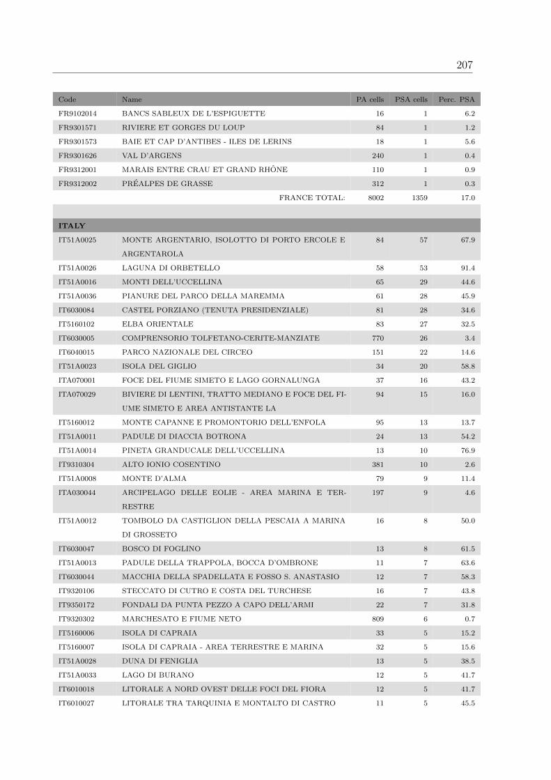
207
Code Name PA cells PSA cells Perc. PSA
FR9102014 BANCS SABLEUX DE L’ESPIGUETTE 16 1 6.2
FR9301571 RIVIERE ET GORGES DU LOUP 84 1 1.2
FR9301573 BAIE ET CAP D’ANTIBES - ILES DE LERINS 18 1 5.6
FR9301626 VAL D’ARGENS 240 1 0.4
FR9312001 MARAIS ENTRE CRAU ET GRAND RHONE 110 1 0.9
FR9312002 PREALPES DE GRASSE 312 1 0.3
FRANCE TOTAL: 8002 1359 17.0
ITALY
IT51A0025 MONTE ARGENTARIO, ISOLOTTO DI PORTO ERCOLE E
ARGENTAROLA
84 57 67.9
IT51A0026 LAGUNA DI ORBETELLO 58 53 91.4
IT51A0016 MONTI DELL’UCCELLINA 65 29 44.6
IT51A0036 PIANURE DEL PARCO DELLA MAREMMA 61 28 45.9
IT6030084 CASTEL PORZIANO (TENUTA PRESIDENZIALE) 81 28 34.6
IT5160102 ELBA ORIENTALE 83 27 32.5
IT6030005 COMPRENSORIO TOLFETANO-CERITE-MANZIATE 770 26 3.4
IT6040015 PARCO NAZIONALE DEL CIRCEO 151 22 14.6
IT51A0023 ISOLA DEL GIGLIO 34 20 58.8
ITA070001 FOCE DEL FIUME SIMETO E LAGO GORNALUNGA 37 16 43.2
ITA070029 BIVIERE DI LENTINI, TRATTO MEDIANO E FOCE DEL FI-
UME SIMETO E AREA ANTISTANTE LA
94 15 16.0
IT5160012 MONTE CAPANNE E PROMONTORIO DELL’ENFOLA 95 13 13.7
IT51A0011 PADULE DI DIACCIA BOTRONA 24 13 54.2
IT51A0014 PINETA GRANDUCALE DELL’UCCELLINA 13 10 76.9
IT9310304 ALTO IONIO COSENTINO 381 10 2.6
IT51A0008 MONTE D’ALMA 79 9 11.4
ITA030044 ARCIPELAGO DELLE EOLIE - AREA MARINA E TER-
RESTRE
197 9 4.6
IT51A0012 TOMBOLO DA CASTIGLION DELLA PESCAIA A MARINA
DI GROSSETO
16 8 50.0
IT6030047 BOSCO DI FOGLINO 13 8 61.5
IT51A0013 PADULE DELLA TRAPPOLA, BOCCA D’OMBRONE 11 7 63.6
IT6030044 MACCHIA DELLA SPADELLATA E FOSSO S. ANASTASIO 12 7 58.3
IT9320106 STECCATO DI CUTRO E COSTA DEL TURCHESE 16 7 43.8
IT9350172 FONDALI DA PUNTA PEZZO A CAPO DELL’ARMI 22 7 31.8
IT9320302 MARCHESATO E FIUME NETO 809 6 0.7
IT5160006 ISOLA DI CAPRAIA 33 5 15.2
IT5160007 ISOLA DI CAPRAIA - AREA TERRESTRE E MARINA 32 5 15.6
IT51A0028 DUNA DI FENIGLIA 13 5 38.5
IT51A0033 LAGO DI BURANO 12 5 41.7
IT6010018 LITORALE A NORD OVEST DELLE FOCI DEL FIORA 12 5 41.7
IT6010027 LITORALE TRA TARQUINIA E MONTALTO DI CASTRO 11 5 45.5

208 APPENDIX C. PROTECTED RANGE SIZES OF SCI
Code Name PA cells PSA cells Perc. PSA
IT6030023 MACCHIA GRANDE DI FOCENE E MACCHIA DELLO STAG-
NETO
7 5 71.4
IT6030027 CASTEL PORZIANO (FASCIA COSTIERA) 14 5 35.7
IT6040012 LAGHI FOGLIANO, MONACI, CAPROLACE E PANTANI
DELL’INFERNO
34 5 14.7
IT9310042 FIUMARA SARACENO 27 5 18.5
ITA030012 LAGUNA DI OLIVERI - TINDARI 9 5 55.6
IT51A0006 PADULE DI SCARLINO 5 4 80.0
IT6030026 LAGO DI TRAIANO 4 4 100.0
IT6040017 PROMONTORIO DEL CIRCEO (QUARTO FREDDO) 14 4 28.6
IT6040018 DUNE DEL CIRCEO 33 4 12.1
IT9310044 FOCE DEL FIUME CRATI 10 4 40.0
IT9350145 FIUMARA AMENDOLEA (INCLUSO ROGHUDI, CHORIO E
ROTA GRECO)
25 4 16.0
IT9350146 FIUMARA BUONAMICO 30 4 13.3
IT9350147 FIUMARA LAVERDE 19 4 21.1
IT9350160 SPIAGGIA DI BRANCALEONE 5 4 80.0
ITA030033 CAPO CALAVA 6 4 66.7
ITA070028 FONDALI DI ACICASTELLO (ISOLA LACHEA - CICLOPI) 7 4 57.1
IT51A0015 DUNE COSTIERE DEL PARCO DELL’UCCELLINA 10 3 30.0
IT51A0024 ISOLA DI GIANNUTRI 10 3 30.0
IT51A0029 BOSCHI DELLE COLLINE DI CAPALBIO 87 3 3.4
IT51A0037 ISOLA DI GIANNUTRI - AREA TERRESTRE E MARINA 10 3 30.0
IT6010019 PIAN DEI CANGANI 4 3 75.0
IT6010026 SALINE DI TARQUINIA 6 3 50.0
IT6030019 MACCHIATONDA 6 3 50.0
IT6030045 LIDO DEI GIGLI 6 3 50.0
IT6040013 LAGO DI SABAUDIA 16 3 18.8
IT9350144 CALANCHI DI PALIZZI MARINA 5 3 60.0
ITA030027 ISOLA DI VULCANO 33 3 9.1
ITA090014 SALINE DI AUGUSTA 3 3 100.0
ITA090026 FONDALI DI BRUCOLI - AGNONE 12 3 25.0
IT5160009 PROMONTORIO DI PIOMBINO E MONTE MASSONCELLO 16 2 12.5
IT5160010 PADULE ORTI - BOTTAGONE 4 2 50.0
IT51A0030 LAGO ACQUATO, LAGO SAN FLORIANO 7 2 28.6
IT51A0031 LAGO DI BURANO 7 2 28.6
IT6030004 VALLE DI RIO FIUME 26 2 7.7
IT6030020 TORRE FLAVIA 3 2 66.7
IT6030046 TOR CALDARA (ZONA SOLFATARE E FOSSI) 2 2 100.0
IT6030048 LITORALE DI TORRE ASTURA 15 2 13.3
IT6030049 ZONE UMIDE A OVEST DEL FIUME ASTURA 3 2 66.7
IT6040016 PROMONTORIO DEL CIRCEO (QUARTO CALDO) 12 2 16.7
IT6040043 MONTI AUSONI E AURUNCI 776 2 0.3

209
Code Name PA cells PSA cells Perc. PSA
IT8010021 PINETA DI PATRIA 11 2 18.2
IT8030010 FONDALI MARINI DI ISCHIA, PROCIDA E VIVARA 69 2 2.9
IT8030018 LAGO DI PATRIA 14 2 14.3
IT9150002 COSTA OTRANTO - SANTA MARIA DI LEUCA 74 2 2.7
IT9220080 COSTA IONICA FOCE AGRI 17 2 11.8
IT9310043 FIUMARA AVENA 22 2 9.1
IT9350132 FIUMARA DI MELITO 8 2 25.0
IT9350138 CALANCHI DI MARO SIMONE 4 2 50.0
IT9350142 CAPO SPARTIVENTO 4 2 50.0
IT9350148 FIUMARA DI PALIZZI 7 2 28.6
ITA010001 ISOLE DELLO STAGNONE DI MARSALA 19 2 10.5
ITA010026 FONDALI DELL’ISOLA DELLO STAGNONE DI MARSALA 16 2 12.5
ITA010028 STAGNONE DI MARSALA E SALINE DI TRAPANI - AREA
MARINA E TERRESTRE
55 2 3.6
ITA030030 ISOLA DI LIPARI 53 2 3.8
ITA030031 ISOLA BELLA, CAPO TAORMINA E CAPO S. ANDREA 2 2 100.0
ITA030040 FONDALI DI TAORMINA - ISOLA BELLA 3 2 66.7
ITA070003 LA GURNA 4 2 50.0
ITA070004 TIMPA DI ACIREALE 13 2 15.4
IT1324909 TORRENTE ARROSCIA E CENTA 15 1 6.7
IT1325624 CAPO MELE 7 1 14.3
IT51A0007 PUNTA ALA E ISOLOTTO DELLO SPARVIERO 11 1 9.1
IT51A0032 DUNA DEL LAGO DI BURANO 7 1 14.3
IT6030016 ANTICA LAVINIUM - PRATICA DI MARE 3 1 33.3
IT6030022 BOSCO DI PALO LAZIALE 5 1 20.0
IT6030024 ISOLA SACRA 3 1 33.3
IT6040019 ISOLE DI PONZA, PALMAROLA, ZANNONE, VENTOTENE
E S. STEFANO
41 1 2.4
IT6040022 COSTA ROCCIOSA TRA SPERLONGA E GAETA 19 1 5.3
IT6040023 PROMONTORIO GIANOLA E MONTE DI SCAURI 7 1 14.3
IT6040024 RIO S. CROCE 5 1 20.0
IT8010019 PINETA DELLA FOCE DEL GARIGLIANO 7 1 14.3
IT8010020 PINETA DI CASTELVOLTURNO 4 1 25.0
IT9150009 LITORALE DI UGENTO 27 1 3.7
IT9210160 ISOLA DI S. IANNI E COSTA PROSPICIENTE 9 1 11.1
IT9310052 CASONI DI SIBARI 9 1 11.1
IT9320102 DUNE DI SOVERETO 6 1 16.7
IT9330105 FOCE DEL CROCCHIO - CROPANI 4 1 25.0
IT9350141 CAPO S. GIOVANNI 2 1 50.0
IT9350171 SPIAGGIA DI PILATI 1 1 100.0
ITA010021 SALINE DI MARSALA 14 1 7.1
ITA030028 ISOLA DI SALINA (MONTE FOSSA DELLE FELCI E DEI
PORRI)
15 1 6.7

210 APPENDIX C. PROTECTED RANGE SIZES OF SCI
Code Name PA cells PSA cells Perc. PSA
ITA090013 SALINE DI PRIOLO 3 1 33.3
ITALY TOTAL: 5266 654 12.4
PORTUGAL
PTCON0018 BARRINHA DE ESMORIZ 10 3 30.0
PTZPE0004 RIA DE AVEIRO 425 2 0.5
PORTUGAL TOTAL: 435 5 1.1
OVERALL NATURA 2000 TOTAL: 20166 5127 25.4
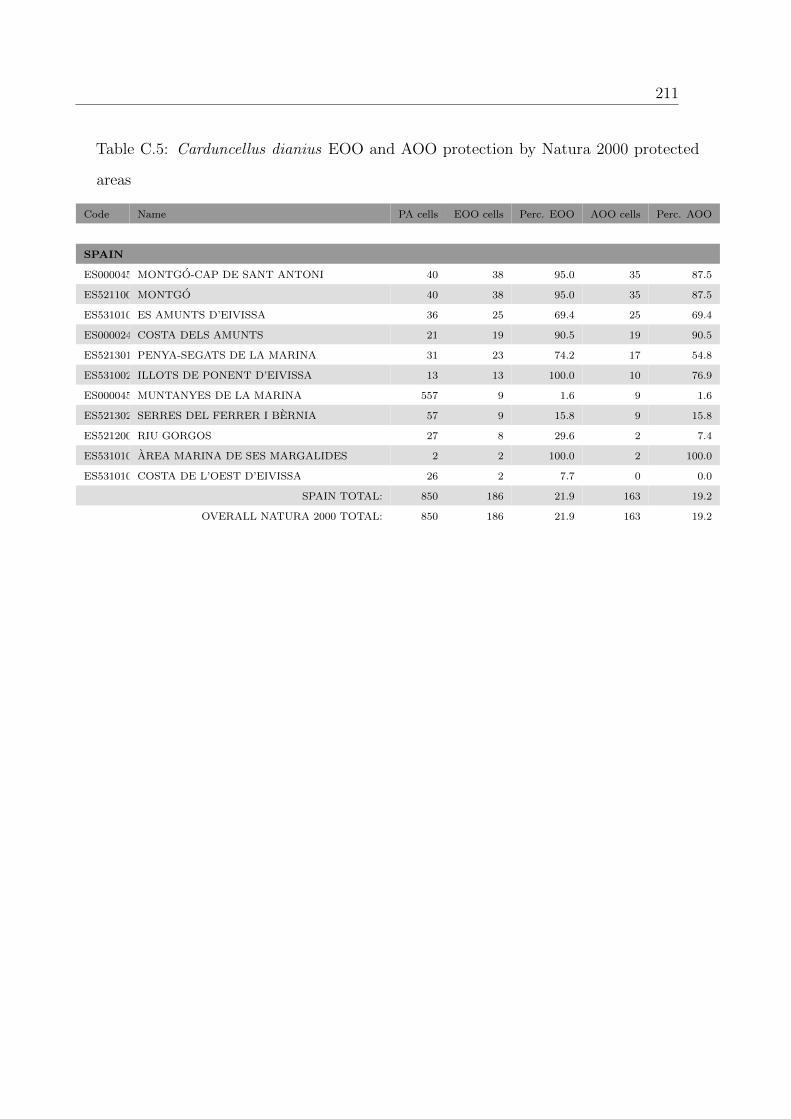
211
Table C.5: Carduncellus dianius EOO and AOO protection by Natura 2000 protected
areas
Code Name PA cells EOO cells Perc. EOO AOO cells Perc. AOO
SPAIN
ES0000454MONTGO-CAP DE SANT ANTONI 40 38 95.0 35 87.5
ES5211007MONTGO 40 38 95.0 35 87.5
ES5310105ES AMUNTS D’EIVISSA 36 25 69.4 25 69.4
ES0000241COSTA DELS AMUNTS 21 19 90.5 19 90.5
ES5213018PENYA-SEGATS DE LA MARINA 31 23 74.2 17 54.8
ES5310023ILLOTS DE PONENT D’EIVISSA 13 13 100.0 10 76.9
ES0000453MUNTANYES DE LA MARINA 557 9 1.6 9 1.6
ES5213020SERRES DEL FERRER I BERNIA 57 9 15.8 9 15.8
ES5212004RIU GORGOS 27 8 29.6 2 7.4
ES5310106AREA MARINA DE SES MARGALIDES 2 2 100.0 2 100.0
ES5310104COSTA DE L’OEST D’EIVISSA 26 2 7.7 0 0.0
SPAIN TOTAL: 850 186 21.9 163 19.2
OVERALL NATURA 2000 TOTAL: 850 186 21.9 163 19.2

212 APPENDIX C. PROTECTED RANGE SIZES OF SCI
Table C.6: Carduncellus dianius PSA protection by North African protected areas
Code Type Name PA cells PSA cells Perc. PSA
ALGERIA
26620 UNESCO-MAB Biosphere
Reserve
El Kala 897 7 0.8
9741 National Park El Kala 897 7 0.8
14909 Marine Park El Kala 897 7 0.8
902531 UNESCO-MAB Biosphere
Reserve
Gouraya 18 6 33.3
9747 National Park Gouraya 18 6 33.3
72362 National Park Tigzirt 3 3 100.0
ALGERIA TOTAL: 2730 36 1.3
TUNISIA
903084 Wetlands of International
Importance (Ramsar)
Sebkhet Kelbia 238 20 8.4
15185 Wetland Zone of National
Importance
Sebkhet Kelbia 238 20 8.4
12390 National Park Boukornine 24 2 8.3
903087 Wetlands of International
Importance (Ramsar)
Sebkhet Soliman 14 2 14.3
15194 Wetland Zone of National
Importance
Sebkha Halk el Menzel 20 1 5.0
TUNISIA TOTAL: 534 45 8.4
OVERALL NORTH AFRICAN TOTAL: 3264 81 2.5
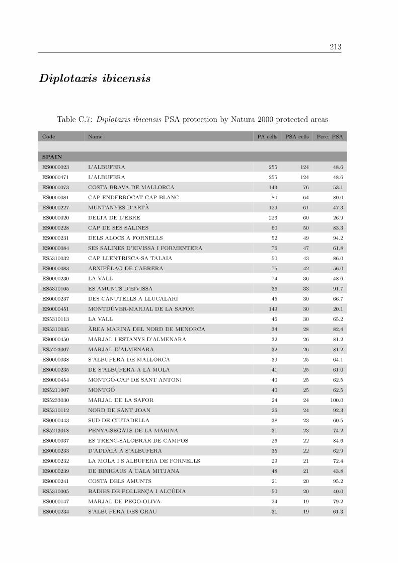
213
Diplotaxis ibicensis
Table C.7: Diplotaxis ibicensis PSA protection by Natura 2000 protected areas
Code Name PA cells PSA cells Perc. PSA
SPAIN
ES0000023 L’ALBUFERA 255 124 48.6
ES0000471 L’ALBUFERA 255 124 48.6
ES0000073 COSTA BRAVA DE MALLORCA 143 76 53.1
ES0000081 CAP ENDERROCAT-CAP BLANC 80 64 80.0
ES0000227 MUNTANYES D’ARTA 129 61 47.3
ES0000020 DELTA DE L’EBRE 223 60 26.9
ES0000228 CAP DE SES SALINES 60 50 83.3
ES0000231 DELS ALOCS A FORNELLS 52 49 94.2
ES0000084 SES SALINES D’EIVISSA I FORMENTERA 76 47 61.8
ES5310032 CAP LLENTRISCA-SA TALAIA 50 43 86.0
ES0000083 ARXIPELAG DE CABRERA 75 42 56.0
ES0000230 LA VALL 74 36 48.6
ES5310105 ES AMUNTS D’EIVISSA 36 33 91.7
ES0000237 DES CANUTELLS A LLUCALARI 45 30 66.7
ES0000451 MONTDUVER-MARJAL DE LA SAFOR 149 30 20.1
ES5310113 LA VALL 46 30 65.2
ES5310035 AREA MARINA DEL NORD DE MENORCA 34 28 82.4
ES0000450 MARJAL I ESTANYS D’ALMENARA 32 26 81.2
ES5223007 MARJAL D’ALMENARA 32 26 81.2
ES0000038 S’ALBUFERA DE MALLORCA 39 25 64.1
ES0000235 DE S’ALBUFERA A LA MOLA 41 25 61.0
ES0000454 MONTGO-CAP DE SANT ANTONI 40 25 62.5
ES5211007 MONTGO 40 25 62.5
ES5233030 MARJAL DE LA SAFOR 24 24 100.0
ES5310112 NORD DE SANT JOAN 26 24 92.3
ES0000443 SUD DE CIUTADELLA 38 23 60.5
ES5213018 PENYA-SEGATS DE LA MARINA 31 23 74.2
ES0000037 ES TRENC-SALOBRAR DE CAMPOS 26 22 84.6
ES0000233 D’ADDAIA A S’ALBUFERA 35 22 62.9
ES0000232 LA MOLA I S’ALBUFERA DE FORNELLS 29 21 72.4
ES0000239 DE BINIGAUS A CALA MITJANA 48 21 43.8
ES0000241 COSTA DELS AMUNTS 21 20 95.2
ES5310005 BADIES DE POLLENCA I ALCUDIA 50 20 40.0
ES0000147 MARJAL DE PEGO-OLIVA. 24 19 79.2
ES0000234 S’ALBUFERA DES GRAU 31 19 61.3

214 APPENDIX C. PROTECTED RANGE SIZES OF SCI
Code Name PA cells PSA cells Perc. PSA
ES0000238 SON BOU I BARRANC DE SA VALL 29 19 65.5
ES5310029 NA BORGES 69 19 27.5
ES0000121 ILLOTS DE BENIDORM I SERRA GELADA 27 18 66.7
ES0000453 MUNTANYES DE LA MARINA 557 17 3.1
ES5222005 MARJAL DE NULES 19 17 89.5
ES5310024 LA MOLA 27 17 63.0
ES5213021 SERRA GELADA I LITORAL DE LA MARINA BAIXA 25 16 64.0
ES5310033 XARRACA 19 16 84.2
ES0000120 SALINAS DE SANTA POLA. 44 15 34.1
ES0000148 MARJAL DELS MOROS. 15 15 100.0
ES0000470 MARJAL DELS MOROS 15 15 100.0
ES0000074 CAP DE CALA FIGUERA 20 14 70.0
ES0000145 MONDRAGO 15 14 93.3
ES0000229 COSTA NORD DE CIUTADELLA 17 14 82.4
ES0000240 COSTA SUD DE CIUTADELLA 25 14 56.0
ES5310078 DE CALA DE SES ORTIGUES A CALA ESTELLENCS 23 13 56.5
ES0000060 PRAT DE CABANES I TORREBLANCA. 18 12 66.7
ES0000459 IFAC I LITORAL DE LA MARINA 14 12 85.7
ES0000467 PRAT DE CABANES I TORREBLANCA 18 12 66.7
ES5211009 IFAC 14 12 85.7
ES5213020 SERRES DEL FERRER I BERNIA 57 12 21.1
ES5310030 COSTA DE LLEVANT 28 12 42.9
ES5310098 CALES DE MANACOR 16 12 75.0
ES0000079 LA VICTORIA 16 11 68.8
ES5310034 SERRA GROSSA 25 11 44.0
ES5310104 COSTA DE L’OEST D’EIVISSA 26 11 42.3
ES5310023 ILLOTS DE PONENT D’EIVISSA 13 10 76.9
ES5310025 CAP DE BARBARIA 18 10 55.6
ES5310081 PORT DES CANONGE 14 10 71.4
ES0000226 L’ALBUFERETA 10 9 90.0
ES5310068 CAP NEGRE 9 9 100.0
ES5310111 AREA MARINA PLATJA DE MIGJORN 22 9 40.9
ES5213024 TABARCA 24 8 33.3
ES5232007 RIU XUQUER 74 8 10.8
ES5310082 S’ESTACA-PUNTA DE DEIA 13 8 61.5
ES0000444 SERRA D’IRTA 105 7 6.7
ES5213025 DUNES DE GUARDAMAR 19 7 36.8
ES5223036 SERRA D’IRTA 105 7 6.7
ES5233015 SERRES DEL MONTDUVER I MARXUQUERA 122 7 5.7
ES5310074 DE CALA LLUCALARI A CALES COVES 12 7 58.3
ES0000221 SA DRAGONERA 15 6 40.0
ES0000222 LA TRAPA 10 6 60.0
ES0000225 SA COSTERA 14 6 42.9
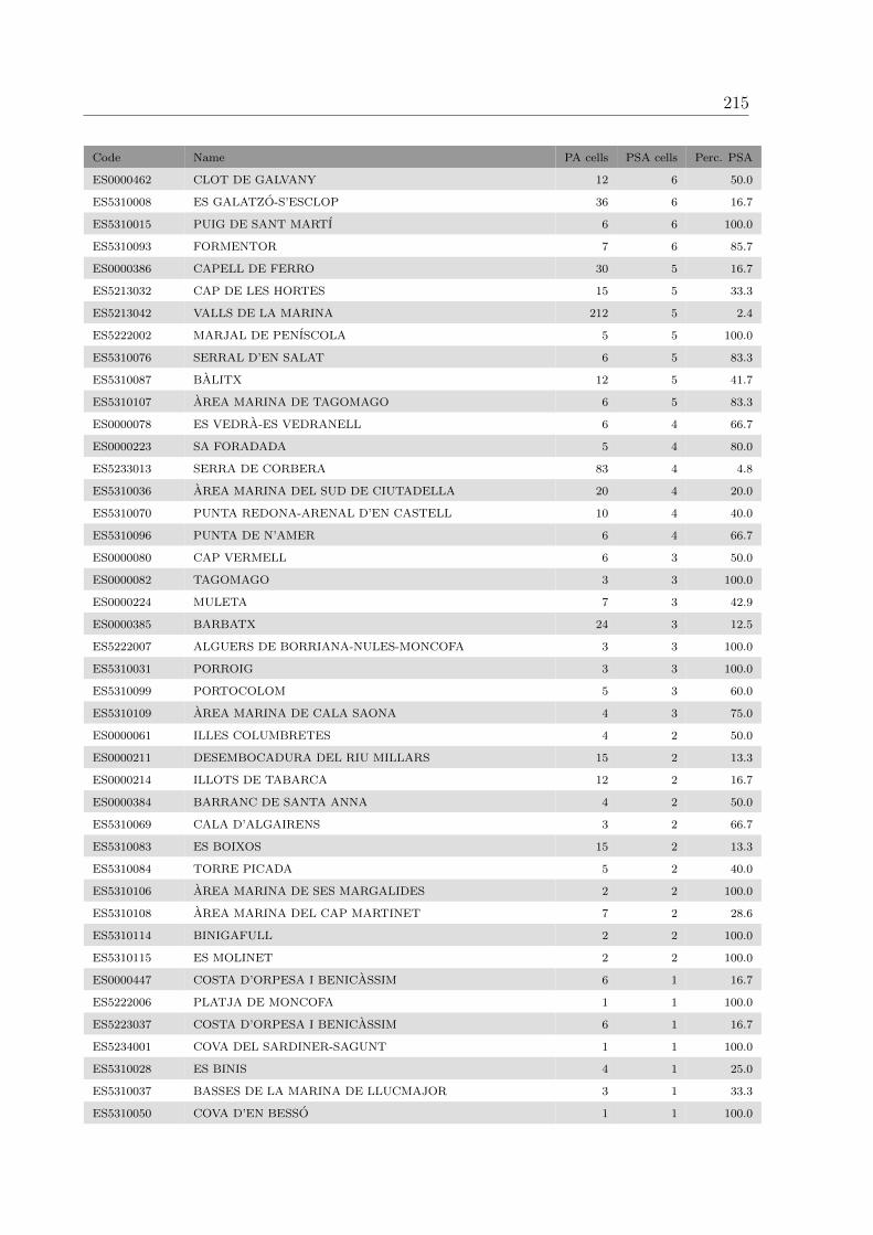
215
Code Name PA cells PSA cells Perc. PSA
ES0000462 CLOT DE GALVANY 12 6 50.0
ES5310008 ES GALATZO-S’ESCLOP 36 6 16.7
ES5310015 PUIG DE SANT MARTI 6 6 100.0
ES5310093 FORMENTOR 7 6 85.7
ES0000386 CAPELL DE FERRO 30 5 16.7
ES5213032 CAP DE LES HORTES 15 5 33.3
ES5213042 VALLS DE LA MARINA 212 5 2.4
ES5222002 MARJAL DE PENISCOLA 5 5 100.0
ES5310076 SERRAL D’EN SALAT 6 5 83.3
ES5310087 BALITX 12 5 41.7
ES5310107 AREA MARINA DE TAGOMAGO 6 5 83.3
ES0000078 ES VEDRA-ES VEDRANELL 6 4 66.7
ES0000223 SA FORADADA 5 4 80.0
ES5233013 SERRA DE CORBERA 83 4 4.8
ES5310036 AREA MARINA DEL SUD DE CIUTADELLA 20 4 20.0
ES5310070 PUNTA REDONA-ARENAL D’EN CASTELL 10 4 40.0
ES5310096 PUNTA DE N’AMER 6 4 66.7
ES0000080 CAP VERMELL 6 3 50.0
ES0000082 TAGOMAGO 3 3 100.0
ES0000224 MULETA 7 3 42.9
ES0000385 BARBATX 24 3 12.5
ES5222007 ALGUERS DE BORRIANA-NULES-MONCOFA 3 3 100.0
ES5310031 PORROIG 3 3 100.0
ES5310099 PORTOCOLOM 5 3 60.0
ES5310109 AREA MARINA DE CALA SAONA 4 3 75.0
ES0000061 ILLES COLUMBRETES 4 2 50.0
ES0000211 DESEMBOCADURA DEL RIU MILLARS 15 2 13.3
ES0000214 ILLOTS DE TABARCA 12 2 16.7
ES0000384 BARRANC DE SANTA ANNA 4 2 50.0
ES5310069 CALA D’ALGAIRENS 3 2 66.7
ES5310083 ES BOIXOS 15 2 13.3
ES5310084 TORRE PICADA 5 2 40.0
ES5310106 AREA MARINA DE SES MARGALIDES 2 2 100.0
ES5310108 AREA MARINA DEL CAP MARTINET 7 2 28.6
ES5310114 BINIGAFULL 2 2 100.0
ES5310115 ES MOLINET 2 2 100.0
ES0000447 COSTA D’ORPESA I BENICASSIM 6 1 16.7
ES5222006 PLATJA DE MONCOFA 1 1 100.0
ES5223037 COSTA D’ORPESA I BENICASSIM 6 1 16.7
ES5234001 COVA DEL SARDINER-SAGUNT 1 1 100.0
ES5310028 ES BINIS 4 1 25.0
ES5310037 BASSES DE LA MARINA DE LLUCMAJOR 3 1 33.3
ES5310050 COVA D’EN BESSO 1 1 100.0
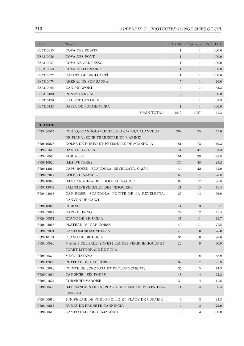
216 APPENDIX C. PROTECTED RANGE SIZES OF SCI
Code Name PA cells PSA cells Perc. PSA
ES5310055 COVA DES PIRATA 1 1 100.0
ES5310056 COVA DES PONT 1 1 100.0
ES5310057 COVA DE CAL PESSO 1 1 100.0
ES5310059 COVA DE LLENAIRE 1 1 100.0
ES5310072 CALETA DE BINILLAUTI 1 1 100.0
ES5310075 ARENAL DE SON SAURA 5 1 20.0
ES5310095 CAN PICAFORT 3 1 33.3
ES5310100 PUNTA DES RAS 2 1 50.0
ES5310120 ES CLOT DES GUIX 3 1 33.3
ES5310123 BASSA DE FORMENTERA 1 1 100.0
SPAIN TOTAL: 4810 1987 41.3
FRANCE
FR9400574 PORTO/SCANDOLA/REVELLATA/CALVI/CALANCHES
DE PIANA (ZONE TERRESTRE ET MARINE)
202 95 47.0
FR9410023 GOLFE DE PORTO ET PRESQU’ILE DE SCANDOLA 181 73 40.3
FR9301613 RADE D’HYERES 141 47 33.3
FR9400570 AGRIATES 151 39 25.8
FR9310020 ILES D’HYERES 130 38 29.2
FR9412010 CAPU ROSSU , SCANDOLA, REVELLATA, CALVI 40 22 55.0
FR9402017 GOLFE D’AJACCIO 66 17 25.8
FR9410096 ILES SANGUINAIRES, GOLFE D’AJACCIO 66 17 25.8
FR9312008 SALINS D’HYERES ET DES PESQUIERS 21 15 71.4
FR9402018 CAP ROSSU, SCANDOLA, POINTE DE LA REVELETTA,
CANYON DE CALVI
25 14 56.0
FR9410098 URBINO 41 13 31.7
FR9402012 CAPO DI FENO 29 12 41.4
FR9400571 ETANG DE BIGUGLIA 37 11 29.7
FR9402013 PLATEAU DU CAP CORSE 40 11 27.5
FR9402001 CAMPOMORO-SENETOSA 40 10 25.0
FR9410101 ETANG DE BIGUGLIA 35 10 28.6
FR9400580 MARAIS DEL SALE, ZONES HUMIDES PERIPHERIQUES ET
FORET LITTORALE DE PINIA
22 9 40.9
FR9400572 MUCCHIATANA 9 8 88.9
FR9412009 PLATEAU DU CAP CORSE 32 7 21.9
FR9402016 POINTE DE SENETOSA ET PROLONGEMENTS 35 5 14.3
FR9301610 CAP SICIE - SIX FOURS 18 4 22.2
FR9301624 CORNICHE VAROISE 34 4 11.8
FR9400595 ILES SANGUINAIRES, PLAGE DE LAVA ET PUNTA PEL-
LUSELLA
11 4 36.4
FR9400616 JUNIPERAIE DE PORTO POLLO ET PLAGE DE CUPABIA 9 3 33.3
FR9400617 DUNES DE PRUNETE-CANNICCIA 4 3 75.0
FR9400619 CAMPO DELL’ORO (AJACCIO) 3 3 100.0

217
Code Name PA cells PSA cells Perc. PSA
FR9400577 RIVIERE ET VALLEE DU FANGO 249 2 0.8
FR9400594 SITES A ANCHUSA CRISPA DE L’EMBOUCHURE DU RIZ-
ZANESE ET D’OLMETO
5 2 40.0
FR9400610 EMBOUCHURE DU TARAVO, PLAGE DE TENUTELLA ET
ETANG DE TANCHICCIA
9 2 22.2
FR9402014 GRAND HERBIER DE LA COTE ORIENTALE 8 2 25.0
FR9400586 EMBOUCHURE DU STABIACCU, DOMAINE PUBLIC MAR-
ITIME ET ILOT ZIGLIONE
6 1 16.7
FR9400593 ROCCAPINA-ORTOLO 24 1 4.2
FR9400599 STRETTES DE ST FLORENT 6 1 16.7
FR9400602 BASSE VALLEE DU TAVIGNANO 55 1 1.8
FRANCE TOTAL: 1784 506 28.4
ITALY
IT51A0025 MONTE ARGENTARIO, ISOLOTTO DI PORTO ERCOLE E
ARGENTAROLA
84 43 51.2
ITB020041 ENTROTERRA E ZONA COSTIERA TRA BOSA, CAPO
MARARGIU E PORTO TANGONE
337 25 7.4
ITA010029 MONTE COFANO, CAPO SAN VITO E MONTE SPARAGIO 218 24 11.0
IT51A0023 ISOLA DEL GIGLIO 34 23 67.6
IT51A0026 LAGUNA DI ORBETELLO 58 23 39.7
ITB010042 CAPO CACCIA (CON LE ISOLE FORADADA E PIANA) E
PUNTA DEL GIGLIO
75 19 25.3
ITB033036 COSTA DI CUGLIERI 41 18 43.9
ITA070001 FOCE DEL FIUME SIMETO E LAGO GORNALUNGA 37 16 43.2
IT6030005 COMPRENSORIO TOLFETANO-CERITE-MANZIATE 770 15 1.9
ITA010028 STAGNONE DI MARSALA E SALINE DI TRAPANI - AREA
MARINA E TERRESTRE
55 15 27.3
ITA070029 BIVIERE DI LENTINI, TRATTO MEDIANO E FOCE DEL FI-
UME SIMETO E AREA ANTISTANTE LA
94 15 16.0
ITB010003 STAGNO E GINEPRETO DI PLATAMONA 28 15 53.6
IT5160012 MONTE CAPANNE E PROMONTORIO DELL’ENFOLA 95 13 13.7
IT5160013 ISOLA DI PIANOSA 21 13 61.9
IT5160016 ISOLA DI PIANOSA - AREA TERRESTRE E MARINA 22 13 59.1
ITB010043 COSTE E ISOLETTE A NORD OVEST DELLA SARDEGNA 48 13 27.1
ITA010017 CAPO SAN VITO, MONTE MONACO, ZINGARO,
FARAGLIONI SCOPELLO, MONTE SPARACIO
108 12 11.1
ITB013044 CAPO CACCIA 51 12 23.5
ITB023037 COSTA E ENTROTERRA DI BOSA, SUNI E MONTRESTA 126 12 9.5
IT5160014 ISOLA DI MONTECRISTO 20 11 55.0
IT5160017 ISOLA DI MONTECRISTO E FORMICA DI MONTECRISTO
- AREA TERRESTRE E MARINA
20 11 55.0
ITA070004 TIMPA DI ACIREALE 13 11 84.6

218 APPENDIX C. PROTECTED RANGE SIZES OF SCI
Code Name PA cells PSA cells Perc. PSA
ITA030044 ARCIPELAGO DELLE EOLIE - AREA MARINA E TER-
RESTRE
197 10 5.1
ITB010004 FOCI DEL COGHINAS 38 10 26.3
ITA010007 SALINE DI TRAPANI 25 9 36.0
IT5160102 ELBA ORIENTALE 83 8 9.6
ITA010016 MONTE COFANO E LITORALE 13 8 61.5
ITB011155 LAGO DI BARATZ - PORTO FERRO 25 8 32.0
IT9320106 STECCATO DI CUTRO E COSTA DEL TURCHESE 16 7 43.8
ITA090008 CAPO MURRO DI PORCO, PENISOLA DELLA MAD-
DALENA E GROTTA PELLEGRINO
9 7 77.8
ITB032228 IS ARENAS 20 7 35.0
IT9320302 MARCHESATO E FIUME NETO 809 6 0.7
ITA010025 FONDALI DEL GOLFO DI CUSTONACI 11 6 54.5
ITA090026 FONDALI DI BRUCOLI - AGNONE 12 6 50.0
ITB010001 ISOLA ASINARA 86 6 7.0
ITB010082 ISOLA DELL’ASINARA 91 6 6.6
IT51A0028 DUNA DI FENIGLIA 13 5 38.5
IT6010018 LITORALE A NORD OVEST DELLE FOCI DEL FIORA 12 5 41.7
ITA010010 MONTE SAN GIULIANO 20 5 25.0
ITA030012 LAGUNA DI OLIVERI - TINDARI 9 5 55.6
ITA030033 CAPO CALAVA 6 5 83.3
ITA070028 FONDALI DI ACICASTELLO (ISOLA LACHEA - CICLOPI) 7 5 71.4
ITB030038 STAGNO DI PUTZU IDU (SALINA MANNA E PAULI
MARIGOSA)
10 5 50.0
ITB040030 CAPO PECORA 55 5 9.1
IT51A0033 LAGO DI BURANO 12 4 33.3
IT9310304 ALTO IONIO COSENTINO 381 4 1.0
IT9350160 SPIAGGIA DI BRANCALEONE 5 4 80.0
ITA010001 ISOLE DELLO STAGNONE DI MARSALA 19 4 21.1
ITA010021 SALINE DI MARSALA 14 4 28.6
ITA010026 FONDALI DELL’ISOLA DELLO STAGNONE DI MARSALA 16 4 25.0
ITA010027 ARCIPELAGO DELLE EGADI - AREA MARINA E TER-
RESTRE
77 4 5.2
ITA020014 MONTE PELLEGRINO 15 4 26.7
ITA030003 RUPI DI TAORMINA E MONTE VENERETTA 14 4 28.6
ITB012211 ISOLA ROSSA - COSTA PARADISO 66 4 6.1
ITB030035 STAGNO DI SALE ’E PORCUS 15 4 26.7
ITB034007 STAGNO DI SALE E’ PORCUS 14 4 28.6
ITB040071 DA PISCINAS A RIU SCIVU 39 4 10.3
IT51A0024 ISOLA DI GIANNUTRI 10 3 30.0
IT51A0037 ISOLA DI GIANNUTRI - AREA TERRESTRE E MARINA 10 3 30.0
IT6010019 PIAN DEI CANGANI 4 3 75.0
IT6010026 SALINE DI TARQUINIA 6 3 50.0
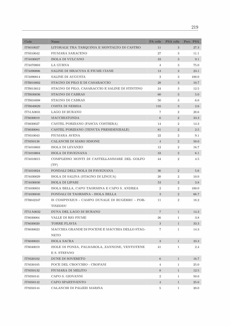
219
Code Name PA cells PSA cells Perc. PSA
IT6010027 LITORALE TRA TARQUINIA E MONTALTO DI CASTRO 11 3 27.3
IT9310042 FIUMARA SARACENO 27 3 11.1
ITA030027 ISOLA DI VULCANO 33 3 9.1
ITA070003 LA GURNA 4 3 75.0
ITA090006 SALINE DI SIRACUSA E FIUME CIANE 13 3 23.1
ITA090014 SALINE DI AUGUSTA 3 3 100.0
ITB010002 STAGNO DI PILO E DI CASARACCIO 28 3 10.7
ITB013012 STAGNO DI PILO, CASARACCIO E SALINE DI STINTINO 24 3 12.5
ITB030036 STAGNO DI CABRAS 60 3 5.0
ITB034008 STAGNO DI CABRAS 50 3 6.0
ITB040029 COSTA DI NEBIDA 116 3 2.6
IT51A0031 LAGO DI BURANO 7 2 28.6
IT6030019 MACCHIATONDA 6 2 33.3
IT6030027 CASTEL PORZIANO (FASCIA COSTIERA) 14 2 14.3
IT6030084 CASTEL PORZIANO (TENUTA PRESIDENZIALE) 81 2 2.5
IT9310043 FIUMARA AVENA 22 2 9.1
IT9350138 CALANCHI DI MARO SIMONE 4 2 50.0
ITA010003 ISOLA DI LEVANZO 12 2 16.7
ITA010004 ISOLA DI FAVIGNANA 33 2 6.1
ITA010015 COMPLESSO MONTI DI CASTELLAMMARE DEL GOLFO
(TP)
44 2 4.5
ITA010024 FONDALI DELL’ISOLA DI FAVIGNANA 36 2 5.6
ITA030029 ISOLA DI SALINA (STAGNO DI LINGUA) 20 2 10.0
ITA030030 ISOLA DI LIPARI 53 2 3.8
ITA030031 ISOLA BELLA, CAPO TAORMINA E CAPO S. ANDREA 2 2 100.0
ITA030040 FONDALI DI TAORMINA - ISOLA BELLA 3 2 66.7
ITB042247 IS COMPINXIUS - CAMPO DUNALE DI BUGERRU - POR-
TIXEDDU
11 2 18.2
IT51A0032 DUNA DEL LAGO DI BURANO 7 1 14.3
IT6030004 VALLE DI RIO FIUME 26 1 3.8
IT6030020 TORRE FLAVIA 3 1 33.3
IT6030023 MACCHIA GRANDE DI FOCENE E MACCHIA DELLO STAG-
NETO
7 1 14.3
IT6030024 ISOLA SACRA 3 1 33.3
IT6040019 ISOLE DI PONZA, PALMAROLA, ZANNONE, VENTOTENE
E S. STEFANO
41 1 2.4
IT9320102 DUNE DI SOVERETO 6 1 16.7
IT9330105 FOCE DEL CROCCHIO - CROPANI 4 1 25.0
IT9350132 FIUMARA DI MELITO 8 1 12.5
IT9350141 CAPO S. GIOVANNI 2 1 50.0
IT9350142 CAPO SPARTIVENTO 4 1 25.0
IT9350144 CALANCHI DI PALIZZI MARINA 5 1 20.0
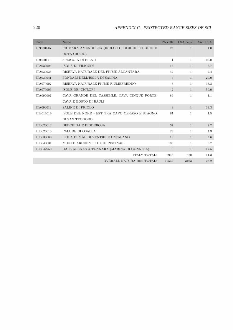
220 APPENDIX C. PROTECTED RANGE SIZES OF SCI
Code Name PA cells PSA cells Perc. PSA
IT9350145 FIUMARA AMENDOLEA (INCLUSO ROGHUDI, CHORIO E
ROTA GRECO)
25 1 4.0
IT9350171 SPIAGGIA DI PILATI 1 1 100.0
ITA030024 ISOLA DI FILICUDI 15 1 6.7
ITA030036 RISERVA NATURALE DEL FIUME ALCANTARA 42 1 2.4
ITA030041 FONDALI DELL’ISOLA DI SALINA 5 1 20.0
ITA070002 RISERVA NATURALE FIUME FIUMEFREDDO 3 1 33.3
ITA070006 ISOLE DEI CICLOPI 2 1 50.0
ITA090007 CAVA GRANDE DEL CASSIBILE, CAVA CINQUE PORTE,
CAVA E BOSCO DI BAULI
89 1 1.1
ITA090013 SALINE DI PRIOLO 3 1 33.3
ITB013019 ISOLE DEL NORD - EST TRA CAPO CERASO E STAGNO
DI SAN TEODORO
67 1 1.5
ITB020012 BERCHIDA E BIDDEROSA 37 1 2.7
ITB020013 PALUDE DI OSALLA 23 1 4.3
ITB030080 ISOLA DI MAL DI VENTRE E CATALANO 18 1 5.6
ITB040031 MONTE ARCUENTU E RIO PISCINAS 138 1 0.7
ITB042250 DA IS ARENAS A TONNARA (MARINA DI GONNESA) 8 1 12.5
ITALY TOTAL: 5948 670 11.3
OVERALL NATURA 2000 TOTAL: 12542 3163 25.2

221
Table C.8: Diplotaxis ibicensis EOO and AOO protection by Natura 2000 protected areas
Code Name PA cells EOO cells Perc. EOO AOO cells Perc. AOO
SPAIN
ES0000081CAP ENDERROCAT-CAP BLANC 80 80 100.0 64 80.0
ES0000084SES SALINES D’EIVISSA I FORMENTERA 76 76 100.0 47 61.8
ES5310032CAP LLENTRISCA-SA TALAIA 50 50 100.0 43 86.0
ES0000083ARXIPELAG DE CABRERA 75 66 88.0 37 49.3
ES5310105ES AMUNTS D’EIVISSA 36 36 100.0 33 91.7
ES5310112NORD DE SANT JOAN 26 26 100.0 24 92.3
ES0000037ES TRENC-SALOBRAR DE CAMPOS 26 26 100.0 22 84.6
ES0000038S’ALBUFERA DE MALLORCA 39 32 82.1 20 51.3
ES0000073COSTA BRAVA DE MALLORCA 143 29 20.3 20 14.0
ES0000241COSTA DELS AMUNTS 21 21 100.0 20 95.2
ES5310033XARRACA 19 19 100.0 16 84.2
ES5213018PENYA-SEGATS DE LA MARINA 31 22 71.0 15 48.4
ES0000074CAP DE CALA FIGUERA 20 20 100.0 14 70.0
ES5310078DE CALA DE SES ORTIGUES A CALA ESTEL-
LENCS
23 23 100.0 13 56.5
ES5310034SERRA GROSSA 25 25 100.0 11 44.0
ES5310104COSTA DE L’OEST D’EIVISSA 26 26 100.0 11 42.3
ES5310023ILLOTS DE PONENT D’EIVISSA 13 13 100.0 10 76.9
ES5310081PORT DES CANONGE 14 14 100.0 10 71.4
ES0000226L’ALBUFERETA 10 10 100.0 9 90.0
ES0000228CAP DE SES SALINES 60 7 11.7 7 11.7
ES5310005BADIES DE POLLENCA I ALCUDIA 50 14 28.0 7 14.0
ES0000221SA DRAGONERA 15 15 100.0 6 40.0
ES0000222LA TRAPA 10 10 100.0 6 60.0
ES5310008ES GALATZO-S’ESCLOP 36 36 100.0 6 16.7
ES5310015PUIG DE SANT MARTI 6 6 100.0 6 100.0
ES5310082S’ESTACA-PUNTA DE DEIA 13 10 76.9 6 46.2
ES5310076SERRAL D’EN SALAT 6 6 100.0 5 83.3
ES5310107AREA MARINA DE TAGOMAGO 6 6 100.0 5 83.3
ES5310111AREA MARINA PLATJA DE MIGJORN 22 10 45.5 5 22.7
ES0000078ES VEDRA-ES VEDRANELL 6 6 100.0 4 66.7
ES0000082TAGOMAGO 3 3 100.0 3 100.0
ES5310025CAP DE BARBARIA 18 3 16.7 3 16.7
ES5310031PORROIG 3 3 100.0 3 100.0
ES5310093FORMENTOR 7 3 42.9 3 42.9
ES5310109AREA MARINA DE CALA SAONA 4 4 100.0 3 75.0
ES0000223SA FORADADA 5 2 40.0 2 40.0
ES5310024LA MOLA 27 3 11.1 2 7.4
ES5310083ES BOIXOS 15 15 100.0 2 13.3

222 APPENDIX C. PROTECTED RANGE SIZES OF SCI
Code Name PA cells EOO cells Perc. EOO AOO cells Perc. AOO
ES5310106AREA MARINA DE SES MARGALIDES 2 2 100.0 2 100.0
ES5310108AREA MARINA DEL CAP MARTINET 7 7 100.0 2 28.6
ES5310037BASSES DE LA MARINA DE LLUCMAJOR 3 3 100.0 1 33.3
ES5310057COVA DE CAL PESSO 1 1 100.0 1 100.0
ES5310059COVA DE LLENAIRE 1 1 100.0 1 100.0
ES5310123BASSA DE FORMENTERA 1 1 100.0 1 100.0
ES0000225SA COSTERA 14 1 7.1 0 0.0
ES0000242ILLOTS DE SANTA EULARIA, RODONA I ES
CANA
2 2 100.0 0 0.0
ES0000377MOLA DE SON PACS 5 5 100.0 0 0.0
ES0000378PUIG DES BOIXOS 7 7 100.0 0 0.0
ES0000379PUIG DE SES FITES 8 8 100.0 0 0.0
ES0000380PUIG DE S’EXTREMERA 4 4 100.0 0 0.0
ES0000381PUIG GROS 20 20 100.0 0 0.0
ES0000382ALARO 4 4 100.0 0 0.0
ES0000383PUIG DES CASTELL 6 6 100.0 0 0.0
ES0000439PLA DE SA MOLA 22 22 100.0 0 0.0
ES0000440DES TEIX AL PUIG DE SES FITES 32 32 100.0 0 0.0
ES0000441D’ALFABIA A BINIARROI 112 112 100.0 0 0.0
ES0000442DE LA SERRA DE L’ESPERO AL PENYAL
ALT
34 34 100.0 0 0.0
ES5310009ES TEIX 18 18 100.0 0 0.0
ES5310010COMUNA DE BUNYOLA 15 15 100.0 0 0.0
ES5310026FITA DES RAM 9 9 100.0 0 0.0
ES5310027CIMALS DE LA SERRA 135 129 95.6 0 0.0
ES5310040COVA DE LES MARAVELLES 1 1 100.0 0 0.0
ES5310042AVENC D’EN CORBERA 1 1 100.0 0 0.0
ES5310048COVA DE SA GUITARRETA 1 1 100.0 0 0.0
ES5310049COVA DES PAS DE VALLGORNERA 1 1 100.0 0 0.0
ES5310058COVA DE CAN SION 1 1 100.0 0 0.0
ES5310060COVA MORELLA 1 1 100.0 0 0.0
ES5310061COVA NOVA DE SON LLUIS 1 1 100.0 0 0.0
ES5310062ES BUFADOR DE SON BERENGUER 1 1 100.0 0 0.0
ES5310063COVA DE CAN MILLO O DE COA NEGRINA 1 1 100.0 0 0.0
ES5310064AVENC DE SON POU 1 1 100.0 0 0.0
ES5310079PUIG DE NA BAUCA 34 34 100.0 0 0.0
ES5310080PUIGPUNYENT 14 14 100.0 0 0.0
ES5310085MONCAIRE 10 4 40.0 0 0.0
ES5310086MONNABER 2 2 100.0 0 0.0
ES5310088GORG BLAU 6 6 100.0 0 0.0
ES5310089BINIARROI 11 11 100.0 0 0.0
ES5310090PUIG D’ALARO-PUIG DE S’ALCADENA 12 12 100.0 0 0.0
ES5310091MOSSA 11 10 90.9 0 0.0

223
Code Name PA cells EOO cells Perc. EOO AOO cells Perc. AOO
ES5310092MUNTANYES DE POLLENCA 54 54 100.0 0 0.0
ES5310101RANDA 23 23 100.0 0 0.0
ES5310102XORRIGO 18 18 100.0 0 0.0
ES5310103AREA MARINA CAP DE CALA FIGUERA 1 1 100.0 0 0.0
SPAIN TOTAL: 1733 1418 81.8 531 30.6
OVERALL NATURA 2000 TOTAL: 1733 1418 81.8 531 30.6

224 APPENDIX C. PROTECTED RANGE SIZES OF SCI
Table C.9: Diplotaxis ibicensis PSA protection by North African protected areas
Code Type Name PA cells PSA cells Perc. PSA
ALGERIA
902531 UNESCO-MAB Biosphere
Reserve
Gouraya 18 9 50.0
9747 National Park Gouraya 18 9 50.0
26620 UNESCO-MAB Biosphere
Reserve
El Kala 897 6 0.7
9741 National Park El Kala 897 6 0.7
14909 Marine Park El Kala 897 6 0.7
72362 National Park Tigzirt 3 3 100.0
ALGERIA TOTAL: 2730 39 1.4
OVERALL NORTH AFRICAN TOTAL: 2730 39 1.4

225
Euphorbia squamigera
Table C.10: Euphoriba squamigera PSA protection by Natura 2000 protected areas
Code Name PA cells PSA cells Perc. PSA
SPAIN
ES0000388 SIERRA DE ALCARAZ Y SEGURA Y CANONES DEL SE-
GURA Y DEL MUNDO
2227 2173 97.6
ES4210008 SIERRA DE ALCARAZ Y SEGURA Y CANONES DEL SE-
GURA Y DEL MUNDO
2213 2159 97.6
ES6140004 SIERRA NEVADA 1925 1925 100.0
ES0000035 SIERRAS DE CAZORLA, SEGURA Y LAS VILLAS 2294 1563 68.1
ES0000212 SIERRA DE MARTES-MUELA DE CORTES 1554 1554 100.0
ES0000449 ALTO TURIA Y SIERRA DEL NEGRETE 1126 897 79.7
ES0000159 HOCES DEL CABRIEL, GUADAZAON Y OJOS DE MOYA 950 804 84.6
ES4230013 HOCES DEL CABRIEL, GUADAZAON Y OJOS DE MOYA 926 780 84.2
ES5233040 MUELA DE CORTES Y EL CAROCHE 690 690 100.0
ES6140001 SIERRA DE BAZA 608 608 100.0
ES6110008 SIERRAS DE GADOR Y ENIX 598 590 98.7
ES6140005 SIERRAS DEL NORDESTE 572 569 99.5
ES0000453 MUNTANYES DE LA MARINA 557 557 100.0
ES5140011 SISTEMA PRELITORAL MERIDIONAL 680 507 74.6
ES6170007 SIERRAS DE TEJEDA, ALMIJARA Y ALHAMA 480 478 99.6
ES0000468 SERRA D’ESPADA 751 451 60.1
ES5233011 SIERRAS DE MARTES Y EL AVE 423 423 100.0
ES0000046 CABO DE GATA-NIJAR 477 416 87.2
ES0000298 MATARRANA - AIGUABARREIX 434 413 95.2
ES6110005 SIERRA DE CABRERA-BEDAR 413 407 98.5
ES0000472 HOCES DEL CABRIEL 401 396 98.8
ES0000153 AREA ESTEPARIA DEL ESTE DE ALBACETE 378 378 100.0
ES0000265 SIERRA DEL MOLINO, EMBALSE DEL QUIPAR Y LLANOS
DEL CAGITAN
340 340 100.0
ES0000262 SIERRAS DEL GIGANTE-PERYCAI, LOMAS DEL BUITRE-
RIO LUCHENA Y SIERRA DE LA TORRECI
332 332 100.0
ES6140008 SIERRA DE LOJA 330 330 100.0
ES0000261 SIERRA DE ALMENARA, MORERAS Y CABO COPE 327 327 100.0
ES6110006 RAMBLAS DE GERGAL, TABERNAS Y SUR DE SIERRA AL-
HAMILLA
324 322 99.4
ES5140009 TIVISSA-VANDELLOS-LLABERIA 321 319 99.4
ES0000031 SIERRA DE GRAZALEMA 609 302 49.6
ES6110003 SIERRA MARIA - LOS VELEZ 295 295 100.0
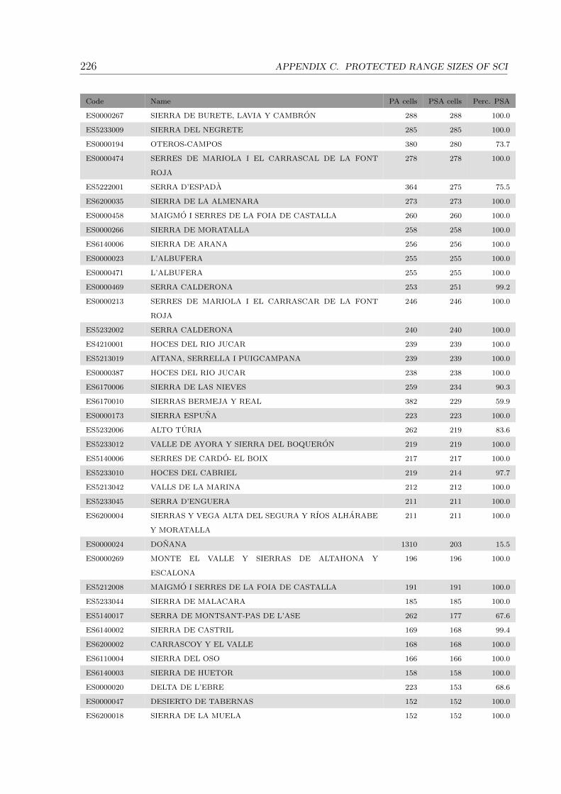
226 APPENDIX C. PROTECTED RANGE SIZES OF SCI
Code Name PA cells PSA cells Perc. PSA
ES0000267 SIERRA DE BURETE, LAVIA Y CAMBRON 288 288 100.0
ES5233009 SIERRA DEL NEGRETE 285 285 100.0
ES0000194 OTEROS-CAMPOS 380 280 73.7
ES0000474 SERRES DE MARIOLA I EL CARRASCAL DE LA FONT
ROJA
278 278 100.0
ES5222001 SERRA D’ESPADA 364 275 75.5
ES6200035 SIERRA DE LA ALMENARA 273 273 100.0
ES0000458 MAIGMO I SERRES DE LA FOIA DE CASTALLA 260 260 100.0
ES0000266 SIERRA DE MORATALLA 258 258 100.0
ES6140006 SIERRA DE ARANA 256 256 100.0
ES0000023 L’ALBUFERA 255 255 100.0
ES0000471 L’ALBUFERA 255 255 100.0
ES0000469 SERRA CALDERONA 253 251 99.2
ES0000213 SERRES DE MARIOLA I EL CARRASCAR DE LA FONT
ROJA
246 246 100.0
ES5232002 SERRA CALDERONA 240 240 100.0
ES4210001 HOCES DEL RIO JUCAR 239 239 100.0
ES5213019 AITANA, SERRELLA I PUIGCAMPANA 239 239 100.0
ES0000387 HOCES DEL RIO JUCAR 238 238 100.0
ES6170006 SIERRA DE LAS NIEVES 259 234 90.3
ES6170010 SIERRAS BERMEJA Y REAL 382 229 59.9
ES0000173 SIERRA ESPUNA 223 223 100.0
ES5232006 ALTO TURIA 262 219 83.6
ES5233012 VALLE DE AYORA Y SIERRA DEL BOQUERON 219 219 100.0
ES5140006 SERRES DE CARDO- EL BOIX 217 217 100.0
ES5233010 HOCES DEL CABRIEL 219 214 97.7
ES5213042 VALLS DE LA MARINA 212 212 100.0
ES5233045 SERRA D’ENGUERA 211 211 100.0
ES6200004 SIERRAS Y VEGA ALTA DEL SEGURA Y RIOS ALHARABE
Y MORATALLA
211 211 100.0
ES0000024 DONANA 1310 203 15.5
ES0000269 MONTE EL VALLE Y SIERRAS DE ALTAHONA Y
ESCALONA
196 196 100.0
ES5212008 MAIGMO I SERRES DE LA FOIA DE CASTALLA 191 191 100.0
ES5233044 SIERRA DE MALACARA 185 185 100.0
ES5140017 SERRA DE MONTSANT-PAS DE L’ASE 262 177 67.6
ES6140002 SIERRA DE CASTRIL 169 168 99.4
ES6200002 CARRASCOY Y EL VALLE 168 168 100.0
ES6110004 SIERRA DEL OSO 166 166 100.0
ES6140003 SIERRA DE HUETOR 158 158 100.0
ES0000020 DELTA DE L’EBRE 223 153 68.6
ES0000047 DESIERTO DE TABERNAS 152 152 100.0
ES6200018 SIERRA DE LA MUELA 152 152 100.0

227
Code Name PA cells PSA cells Perc. PSA
ES5223055 SERRA D’EN GALCERAN 169 151 89.3
ES0000451 MONTDUVER-MARJAL DE LA SAFOR 149 149 100.0
ES6170016 VALLE DEL RIO DEL GENAL 290 149 51.4
ES0000465 L’ALT MAESTRAT, TINENCA DE BENIFASSA, TURMELL I
VALLIVANA
1107 148 13.4
ES0000461 SERRES DEL SUD D’ALACANT 142 142 100.0
ES0000264 SIERRA DE LA MUELA Y CABO TINOSO 147 136 92.5
ES0000464 SIERRA ESCALONA Y DEHESA DE CAMPOAMOR 136 136 100.0
ES6170012 SIERRA DE CAMAROLOS 132 130 98.5
ES5213054 ELS ALFORINS 128 128 100.0
ES6140007 SIERRAS DEL CAMPANARIO Y LAS CABRAS 136 128 94.1
ES6200026 SIERRA DE RICOTE-LA NAVELA 127 127 100.0
ES5233001 TINENCA DE BENIFASSA, TURMELL I VALLIVANA 571 125 21.9
ES5233015 SERRES DEL MONTDUVER I MARXUQUERA 122 122 100.0
ES0000257 SIERRAS DE RICOTE Y LA NAVELA 121 121 100.0
ES6200003 SIERRA DE LA PILA 119 119 100.0
ES0000457 SIERRA DE SALINAS 117 117 100.0
ES0000073 COSTA BRAVA DE MALLORCA 143 116 81.1
ES5213039 SIERRA DE SALINAS 115 115 100.0
ES0000045 SIERRA ALHAMILLA 111 111 100.0
ES0000174 SIERRA DE LA PILA 109 109 100.0
ES6200017 SIERRA DE VILLAFUERTE 109 109 100.0
ES5140012 TOSSALS D’ALMATRET I RIBA ROJA 108 108 100.0
ES2430097 RIO MATARRANYA 106 106 100.0
ES6200045 RIO MULA Y PLIEGO 104 104 100.0
ES6200015 LA MUELA Y CABO TINOSO 110 103 93.6
ES0000452 MECA-MUGRON-SAN BENITO 98 98 100.0
ES0000444 SERRA D’IRTA 105 94 89.5
ES5223036 SERRA D’IRTA 105 94 89.5
ES6110011 SIERRA DEL ALTO DE ALMAGRO 94 94 100.0
ES0000227 MUNTANYES D’ARTA 129 92 71.3
ES0000455 ELS ALFORINS 92 92 100.0
ES6110013 CALARES DE SIERRA DE LOS FILABRES 91 91 100.0
ES0000365 PARAMO LEONES 90 90 100.0
ES6200009 SIERRA DE EL CARCHE 86 86 100.0
ES6110012 SIERRAS ALMAGRERA, DE LOS PINOS Y EL AGUILON 87 84 96.6
ES0000441 D’ALFABIA A BINIARROI 112 83 74.1
ES5233013 SERRA DE CORBERA 83 83 100.0
ES5140005 SERRA DE MONTSIA 83 82 98.8
ES0000049 LOS ALCORNOCALES 1844 81 4.4
ES0000366 VALDERIA-JAMUZ 134 79 59.0
ES5213022 SERRA DE CREVILLENT 78 78 100.0
ES5212012 SIERRA DE ESCALONA Y DEHESA DE CAMPOAMOR 77 77 100.0

228 APPENDIX C. PROTECTED RANGE SIZES OF SCI
Code Name PA cells PSA cells Perc. PSA
ES6200034 LOMAS DEL BUITRE Y RIO LUCHENA 77 77 100.0
ES0000268 SALADARES DEL GUADALENTIN 76 76 100.0
ES0000463 CABECO D’OR I LA GRANA 74 74 100.0
ES5232007 RIU XUQUER 74 74 100.0
ES6200036 SIERRA DEL BUEY 74 74 100.0
ES5120007 CAP DE CREUS 155 73 47.1
ES6200023 SIERRA DE LA TERCIA 73 73 100.0
ES5140015 RIU SIURANA I PLANES DEL PRIORAT 72 71 98.6
ES6170011 SIERRA BLANCA 87 71 81.6
ES4130079 RIBERAS DEL RIO ESLA Y AFLUENTES 146 70 47.9
ES6200014 SALADARES DEL GUADALENTIN 70 70 100.0
ES4230002 SIERRAS DE TALAYUELAS Y ALIAGUILLA 115 69 60.0
ES6200043 RIO QUIPAR 69 69 100.0
ES0000140 BAHIA DE CADIZ 154 68 44.2
ES0000196 ESTEPAS DE YECLA 67 67 100.0
ES6200019 SIERRA DEL GAVILAN 66 66 100.0
ES2420118 RIO ALGARS 65 65 100.0
ES0000081 CAP ENDERROCAT-CAP BLANC 80 64 80.0
ES6200020 CASA ALTA-LAS SALINAS 63 63 100.0
ES6200022 SIERRA DEL GIGANTE 61 61 100.0
ES0000059 LLACUNES DE LA MATA I TORREVIEJA. 60 60 100.0
ES6200016 REVOLCADORES 60 60 100.0
ES0000337 ESTRECHO 160 58 36.2
ES5232003 CURS MITJA DEL RIU PALANCIA 93 58 62.4
ES5213020 SERRES DEL FERRER I BERNIA 57 57 100.0
ES6200047 SIERRA DE LA TORRECILLA 57 57 100.0
ES0000460 RIU MONTNEGRE 56 56 100.0
ES6130002 SIERRA SUBBETICA 386 55 14.2
ES0000230 LA VALL 74 53 71.6
ES4210004 LAGUNAS SALADAS DE PETROLA Y SALOBREJO Y COM-
PLEJO LAGUNAR DE CORRAL RUBIO
53 53 100.0
ES0000019 AIGUAMOLLS DE L’ALT EMPORDA 89 52 58.4
ES0000182 VALCUERNA, SERRETA NEGRA Y LIBEROLA 464 51 11.0
ES0000228 CAP DE SES SALINES 60 51 85.0
ES5140003 RIBERA DE L’ALGARS 51 51 100.0
ES6200011 SIERRA DE LAS MORERAS 50 50 100.0
ES0000231 DELS ALOCS A FORNELLS 52 49 94.2
ES5233041 SERRA DE LA SAFOR 49 49 100.0
ES0000446 DESERT DE LES PALMES 48 48 100.0
ES0000456 MORATILLAS-ALMELA 48 48 100.0
ES6160007 SIERRA MAGINA 243 48 19.8
ES0000084 SES SALINES D’EIVISSA I FORMENTERA 76 47 61.8
ES5221002 DESERT DE LES PALMES 47 47 100.0

229
Code Name PA cells PSA cells Perc. PSA
ES5140023 SECANS DEL MONTSIA 46 46 100.0
ES5310029 NA BORGES 69 46 66.7
ES5310032 CAP LLENTRISCA-SA TALAIA 50 46 92.0
ES6200001 CALBLANQUE, MONTE DE LAS CENIZAS Y PENA DEL
AGUILA
52 45 86.5
ES6200021 SIERRA DE LAVIA 44 44 100.0
ES6110002 KARST EN YESOS DE SORBAS 43 43 100.0
ES0000083 ARXIPELAG DE CABRERA 75 42 56.0
ES6140015 BARRANCOS DEL RIO DE AGUAS BLANCAS 42 42 100.0
ES0000120 SALINAS DE SANTA POLA. 44 41 93.2
ES0000058 EL FONDO D’ELX-CREVILLENT 39 39 100.0
ES0000195 HUMEDAL DE AJAUQUE Y RAMBLA SALADA 39 39 100.0
ES4130065 RIBERAS DEL RIO ORBIGO Y AFLUENTES 126 39 31.0
ES5310113 LA VALL 46 39 84.8
ES6200046 SIERRA DE ENMEDIO 39 39 100.0
ES0000445 PLANIOLS-BENASQUES 38 38 100.0
ES5120016 EL MONTGRI- LES MEDES - EL BAIX TER 77 38 49.4
ES6150005 MARISMAS DE ISLA CRISTINA 43 38 88.4
ES6200029 FRANJA LITORAL SUMERGIDA DE LA REGION DE MUR-
CIA
70 38 54.3
ES0000260 MAR MENOR 67 37 55.2
ES0000454 MONTGO-CAP DE SANT ANTONI 40 37 92.5
ES4210011 SALADARES DE CORDOVILLA Y AGRAMON Y LAGUNA
DE ALBORAJ
37 37 100.0
ES5211007 MONTGO 40 37 92.5
ES5310027 CIMALS DE LA SERRA 135 37 27.4
ES0000038 S’ALBUFERA DE MALLORCA 39 36 92.3
ES0000237 DES CANUTELLS A LLUCALARI 45 36 80.0
ES5310008 ES GALATZO-S’ESCLOP 36 36 100.0
ES6200039 CABEZO DE LA JARA Y RAMBLA DE NOGALTE 36 36 100.0
ES0000217 PENILLANURAS-CAMPOS NORTE 169 35 20.7
ES4230005 SABINARES DE CAMPILLOS-SIERRA Y VALDEMORILLO
DE LA SIERRA
185 35 18.9
ES5213026 SIERRA DE ORIHUELA 35 35 100.0
ES5140002 SERRA DE GODALL 34 34 100.0
ES5222004 CURS ALT DEL RIU MILLARS 165 34 20.6
ES5310079 PUIG DE NA BAUCA 34 34 100.0
ES0000259 SIERRA DE MOJANTES 33 33 100.0
ES0000443 SUD DE CIUTADELLA 38 33 86.8
ES2420099 SIERRA DE VIZCUERNO 35 33 94.3
ES4130145 LAGUNAS DE LOS OTEROS 58 33 56.9
ES5310105 ES AMUNTS D’EIVISSA 36 33 91.7
ES6200005 HUMEDAL DEL AJAUQUE Y RAMBLA SALADA 33 33 100.0
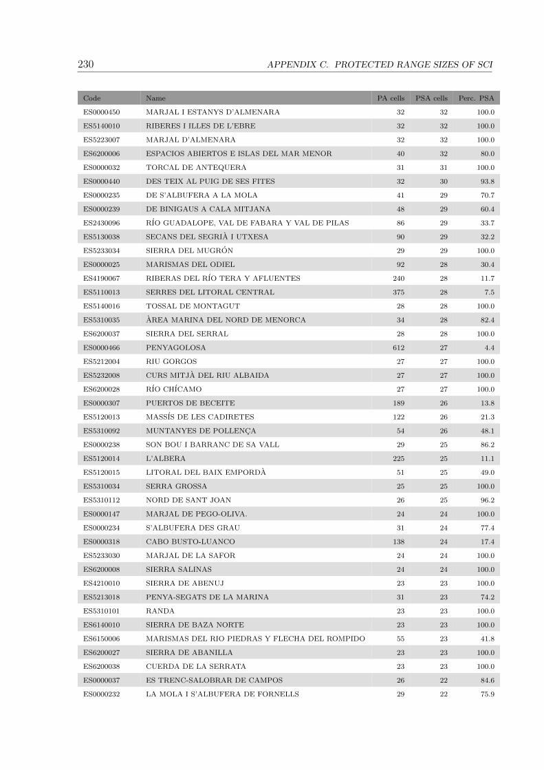
230 APPENDIX C. PROTECTED RANGE SIZES OF SCI
Code Name PA cells PSA cells Perc. PSA
ES0000450 MARJAL I ESTANYS D’ALMENARA 32 32 100.0
ES5140010 RIBERES I ILLES DE L’EBRE 32 32 100.0
ES5223007 MARJAL D’ALMENARA 32 32 100.0
ES6200006 ESPACIOS ABIERTOS E ISLAS DEL MAR MENOR 40 32 80.0
ES0000032 TORCAL DE ANTEQUERA 31 31 100.0
ES0000440 DES TEIX AL PUIG DE SES FITES 32 30 93.8
ES0000235 DE S’ALBUFERA A LA MOLA 41 29 70.7
ES0000239 DE BINIGAUS A CALA MITJANA 48 29 60.4
ES2430096 RIO GUADALOPE, VAL DE FABARA Y VAL DE PILAS 86 29 33.7
ES5130038 SECANS DEL SEGRIA I UTXESA 90 29 32.2
ES5233034 SIERRA DEL MUGRON 29 29 100.0
ES0000025 MARISMAS DEL ODIEL 92 28 30.4
ES4190067 RIBERAS DEL RIO TERA Y AFLUENTES 240 28 11.7
ES5110013 SERRES DEL LITORAL CENTRAL 375 28 7.5
ES5140016 TOSSAL DE MONTAGUT 28 28 100.0
ES5310035 AREA MARINA DEL NORD DE MENORCA 34 28 82.4
ES6200037 SIERRA DEL SERRAL 28 28 100.0
ES0000466 PENYAGOLOSA 612 27 4.4
ES5212004 RIU GORGOS 27 27 100.0
ES5232008 CURS MITJA DEL RIU ALBAIDA 27 27 100.0
ES6200028 RIO CHICAMO 27 27 100.0
ES0000307 PUERTOS DE BECEITE 189 26 13.8
ES5120013 MASSIS DE LES CADIRETES 122 26 21.3
ES5310092 MUNTANYES DE POLLENCA 54 26 48.1
ES0000238 SON BOU I BARRANC DE SA VALL 29 25 86.2
ES5120014 L’ALBERA 225 25 11.1
ES5120015 LITORAL DEL BAIX EMPORDA 51 25 49.0
ES5310034 SERRA GROSSA 25 25 100.0
ES5310112 NORD DE SANT JOAN 26 25 96.2
ES0000147 MARJAL DE PEGO-OLIVA. 24 24 100.0
ES0000234 S’ALBUFERA DES GRAU 31 24 77.4
ES0000318 CABO BUSTO-LUANCO 138 24 17.4
ES5233030 MARJAL DE LA SAFOR 24 24 100.0
ES6200008 SIERRA SALINAS 24 24 100.0
ES4210010 SIERRA DE ABENUJ 23 23 100.0
ES5213018 PENYA-SEGATS DE LA MARINA 31 23 74.2
ES5310101 RANDA 23 23 100.0
ES6140010 SIERRA DE BAZA NORTE 23 23 100.0
ES6150006 MARISMAS DEL RIO PIEDRAS Y FLECHA DEL ROMPIDO 55 23 41.8
ES6200027 SIERRA DE ABANILLA 23 23 100.0
ES6200038 CUERDA DE LA SERRATA 23 23 100.0
ES0000037 ES TRENC-SALOBRAR DE CAMPOS 26 22 84.6
ES0000232 LA MOLA I S’ALBUFERA DE FORNELLS 29 22 75.9
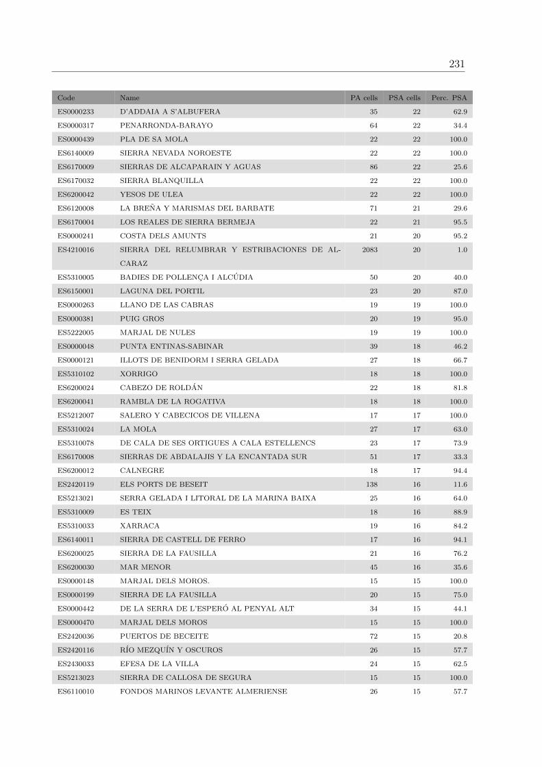
231
Code Name PA cells PSA cells Perc. PSA
ES0000233 D’ADDAIA A S’ALBUFERA 35 22 62.9
ES0000317 PENARRONDA-BARAYO 64 22 34.4
ES0000439 PLA DE SA MOLA 22 22 100.0
ES6140009 SIERRA NEVADA NOROESTE 22 22 100.0
ES6170009 SIERRAS DE ALCAPARAIN Y AGUAS 86 22 25.6
ES6170032 SIERRA BLANQUILLA 22 22 100.0
ES6200042 YESOS DE ULEA 22 22 100.0
ES6120008 LA BRENA Y MARISMAS DEL BARBATE 71 21 29.6
ES6170004 LOS REALES DE SIERRA BERMEJA 22 21 95.5
ES0000241 COSTA DELS AMUNTS 21 20 95.2
ES4210016 SIERRA DEL RELUMBRAR Y ESTRIBACIONES DE AL-
CARAZ
2083 20 1.0
ES5310005 BADIES DE POLLENCA I ALCUDIA 50 20 40.0
ES6150001 LAGUNA DEL PORTIL 23 20 87.0
ES0000263 LLANO DE LAS CABRAS 19 19 100.0
ES0000381 PUIG GROS 20 19 95.0
ES5222005 MARJAL DE NULES 19 19 100.0
ES0000048 PUNTA ENTINAS-SABINAR 39 18 46.2
ES0000121 ILLOTS DE BENIDORM I SERRA GELADA 27 18 66.7
ES5310102 XORRIGO 18 18 100.0
ES6200024 CABEZO DE ROLDAN 22 18 81.8
ES6200041 RAMBLA DE LA ROGATIVA 18 18 100.0
ES5212007 SALERO Y CABECICOS DE VILLENA 17 17 100.0
ES5310024 LA MOLA 27 17 63.0
ES5310078 DE CALA DE SES ORTIGUES A CALA ESTELLENCS 23 17 73.9
ES6170008 SIERRAS DE ABDALAJIS Y LA ENCANTADA SUR 51 17 33.3
ES6200012 CALNEGRE 18 17 94.4
ES2420119 ELS PORTS DE BESEIT 138 16 11.6
ES5213021 SERRA GELADA I LITORAL DE LA MARINA BAIXA 25 16 64.0
ES5310009 ES TEIX 18 16 88.9
ES5310033 XARRACA 19 16 84.2
ES6140011 SIERRA DE CASTELL DE FERRO 17 16 94.1
ES6200025 SIERRA DE LA FAUSILLA 21 16 76.2
ES6200030 MAR MENOR 45 16 35.6
ES0000148 MARJAL DELS MOROS. 15 15 100.0
ES0000199 SIERRA DE LA FAUSILLA 20 15 75.0
ES0000442 DE LA SERRA DE L’ESPERO AL PENYAL ALT 34 15 44.1
ES0000470 MARJAL DELS MOROS 15 15 100.0
ES2420036 PUERTOS DE BECEITE 72 15 20.8
ES2420116 RIO MEZQUIN Y OSCUROS 26 15 57.7
ES2430033 EFESA DE LA VILLA 24 15 62.5
ES5213023 SIERRA DE CALLOSA DE SEGURA 15 15 100.0
ES6110010 FONDOS MARINOS LEVANTE ALMERIENSE 26 15 57.7

232 APPENDIX C. PROTECTED RANGE SIZES OF SCI
Code Name PA cells PSA cells Perc. PSA
ES6140012 LA MALA 15 15 100.0
ES6170003 DESFILADERO DE LOS GAITANES 37 15 40.5
ES0000074 CAP DE CALA FIGUERA 20 14 70.0
ES0000145 MONDRAGO 15 14 93.3
ES0000146 DELTA DEL LLOBREGAT 28 14 50.0
ES0000229 COSTA NORD DE CIUTADELLA 17 14 82.4
ES0000240 COSTA SUD DE CIUTADELLA 25 14 56.0
ES2420114 SALADAS DE ALCANIZ 14 14 100.0
ES5213024 TABARCA 24 14 58.3
ES5213025 DUNES DE GUARDAMAR 19 14 73.7
ES5310080 PUIGPUNYENT 14 14 100.0
ES5310083 ES BOIXOS 15 14 93.3
ES6200040 CABEZOS DEL PERICON 14 14 100.0
ES6150004 LAGUNAS DE PALOS Y LAS MADRES 16 13 81.2
ES0000060 PRAT DE CABANES I TORREBLANCA. 18 12 66.7
ES0000175 SALINAS Y ARENALES DE SAN PEDRO DEL PINATAR 17 12 70.6
ES0000459 IFAC I LITORAL DE LA MARINA 14 12 85.7
ES0000462 CLOT DE GALVANY 12 12 100.0
ES0000467 PRAT DE CABANES I TORREBLANCA 18 12 66.7
ES5211009 IFAC 14 12 85.7
ES5310010 COMUNA DE BUNYOLA 15 12 80.0
ES5310030 COSTA DE LLEVANT 28 12 42.9
ES5310098 CALES DE MANACOR 16 12 75.0
ES6110007 LA SERRETA DE CABO DE GATA 12 12 100.0
ES6110014 ARTOS DE EL EJIDO 12 12 100.0
ES0000079 LA VICTORIA 16 11 68.8
ES0000162 SERRANIA DE CUENCA 2235 11 0.5
ES0000211 DESEMBOCADURA DEL RIU MILLARS 15 11 73.3
ES0000225 SA COSTERA 14 11 78.6
ES4230014 SERRANIA DE CUENCA 2187 11 0.5
ES5310091 MOSSA 11 11 100.0
ES5310104 COSTA DE L’OEST D’EIVISSA 26 11 42.3
ES6310001 CALAMOCARRO-BENZU 11 11 100.0
ES4190134 LAGUNAS DE TERA Y VIDRIALES 47 10 21.3
ES5310023 ILLOTS DE PONENT D’EIVISSA 13 10 76.9
ES5310025 CAP DE BARBARIA 18 10 55.6
ES5310081 PORT DES CANONGE 14 10 71.4
ES5310085 MONCAIRE 10 10 100.0
ES5310087 BALITX 12 10 83.3
ES0000226 L’ALBUFERETA 10 9 90.0
ES2410030 SERRETA NEGRA 188 9 4.8
ES5140001 LITORAL MERIDIONAL TARRAGONI 20 9 45.0
ES5140022 BARRANC DE SANTES CREUS 9 9 100.0

233
Code Name PA cells PSA cells Perc. PSA
ES5310026 FITA DES RAM 9 9 100.0
ES5310068 CAP NEGRE 9 9 100.0
ES5310082 S’ESTACA-PUNTA DE DEIA 13 9 69.2
ES5310111 AREA MARINA PLATJA DE MIGJORN 22 9 40.9
ES6110018 RIO ADRA 9 9 100.0
ES0000379 PUIG DE SES FITES 8 8 100.0
ES0000386 CAPELL DE FERRO 30 8 26.7
ES2410084 LIBEROLA-SERRETA NEGRA 86 8 9.3
ES5212006 LAGUNA DE SALINAS 8 8 100.0
ES5310090 PUIG D’ALARO-PUIG DE S’ALCADENA 12 8 66.7
ES6200044 SIERRA DE LAS VICTORIAS 8 8 100.0
ES0000378 PUIG DES BOIXOS 7 7 100.0
ES5110011 SERRES DEL LITORAL SEPTENTRIONAL 308 7 2.3
ES5212009 ALGEPSARS DE FINESTRAT 7 7 100.0
ES5213033 CABO ROIG 11 7 63.6
ES5310074 DE CALA LLUCALARI A CALES COVES 12 7 58.3
ES6110017 RIO ANTAS 7 7 100.0
ES6120013 SIERRA LIJAR 109 7 6.4
ES6150012 DEHESA DEL ESTERO Y MONTES DE MOGUER 49 7 14.3
ES6150019 BAJO GUADALQUIVIR 160 7 4.4
ES6200013 CABEZO GORDO 7 7 100.0
ES0000021 SECANS DE MAS DE MELONS-ALFES 94 6 6.4
ES0000207 PENILLANURAS-CAMPOS SUR 288 6 2.1
ES0000221 SA DRAGONERA 15 6 40.0
ES0000222 LA TRAPA 10 6 60.0
ES0000385 BARBATX 24 6 25.0
ES1120005 AS CATEDRAIS 17 6 35.3
ES5130040 SECANS DE MAS DE MELONS-ALFES 94 6 6.4
ES5140007 COSTES DEL TARRAGONES 14 6 42.9
ES5310015 PUIG DE SANT MARTI 6 6 100.0
ES5310093 FORMENTOR 7 6 85.7
ES6150003 ESTERO DE DOMINGO RUBIO 13 6 46.2
ES6200031 CABO COPE 6 6 100.0
ES0000377 MOLA DE SON PACS 5 5 100.0
ES0000383 PUIG DES CASTELL 6 5 83.3
ES5120010 LES GAVARRES 344 5 1.5
ES5213032 CAP DE LES HORTES 15 5 33.3
ES5222002 MARJAL DE PENISCOLA 5 5 100.0
ES5310076 SERRAL D’EN SALAT 6 5 83.3
ES5310107 AREA MARINA DE TAGOMAGO 6 5 83.3
ES6150029 ESTUARIO DEL RIO TINTO 18 5 27.8
ES6170005 SIERRA CRESTELLINA 12 5 41.7
ES6200010 CUATRO CALAS 6 5 83.3

234 APPENDIX C. PROTECTED RANGE SIZES OF SCI
Code Name PA cells PSA cells Perc. PSA
ES6200048 MEDIO MARINO 15 5 33.3
ES0000004 LAGUNAS DE VILLAFAFILA 375 4 1.1
ES0000078 ES VEDRA-ES VEDRANELL 6 4 66.7
ES0000223 SA FORADADA 5 4 80.0
ES0000380 PUIG DE S’EXTREMERA 4 4 100.0
ES0000382 ALARO 4 4 100.0
ES0000384 BARRANC DE SANTA ANNA 4 4 100.0
ES5110007 RIU I ESTANYS DE TORDERA 38 4 10.5
ES5140014 MASSIS DE BONASTRE 45 4 8.9
ES5140019 RIU GAIA 67 4 6.0
ES5233047 ULLALS DEL RIU VERD 4 4 100.0
ES5310028 ES BINIS 4 4 100.0
ES5310036 AREA MARINA DEL SUD DE CIUTADELLA 20 4 20.0
ES5310070 PUNTA REDONA-ARENAL D’EN CASTELL 10 4 40.0
ES5310096 PUNTA DE N’AMER 6 4 66.7
ES6110001 ALBUFERA DE ADRA 4 4 100.0
ES6150015 ISLA DE SAN BRUNO 8 4 50.0
ES6150018 RIO GUADIANA Y RIBERA DE CHANZA 97 4 4.1
ES6160008 CUENCAS DEL RUMBLAR, GUADALEN Y GUADALMENA 2071 4 0.2
ES6320002 BARRANCO DEL NANO 4 4 100.0
ES0000080 CAP VERMELL 6 3 50.0
ES0000082 TAGOMAGO 3 3 100.0
ES0000085 RIBADEO 39 3 7.7
ES0000224 MULETA 7 3 42.9
ES1200016 RIA DEL EO 33 3 9.1
ES5120011 RIBERES DEL BAIX TER 80 3 3.8
ES5140008 MUNTANYES DE PRADES 379 3 0.8
ES5222007 ALGUERS DE BORRIANA-NULES-MONCOFA 3 3 100.0
ES5310031 PORROIG 3 3 100.0
ES5310037 BASSES DE LA MARINA DE LLUCMAJOR 3 3 100.0
ES5310089 BINIARROI 11 3 27.3
ES5310099 PORTOCOLOM 5 3 60.0
ES5310109 AREA MARINA DE CALA SAONA 4 3 75.0
ES6120006 MARISMAS DEL RIO PALMONES 4 3 75.0
ES6120017 PUNTA DE TRAFALGAR 7 3 42.9
ES6150002 ENEBRALES DE PUNTA UMBRIA 7 3 42.9
ES6150028 ESTUARIO DEL RIO PIEDRAS 14 3 21.4
ES6170002 ACANTILADOS DE MARO-CERRO GORDO 15 3 20.0
ES0000061 ILLES COLUMBRETES 4 2 50.0
ES0000214 ILLOTS DE TABARCA 12 2 16.7
ES1120011 RIA DE FOZ - MASMA 26 2 7.7
ES5110020 COSTES DEL GARRAF 12 2 16.7
ES5140004 SEQUIA MAJOR 4 2 50.0

235
Code Name PA cells PSA cells Perc. PSA
ES5232005 LAVAJOS DE SINARCAS 2 2 100.0
ES5310069 CALA D’ALGAIRENS 3 2 66.7
ES5310084 TORRE PICADA 5 2 40.0
ES5310086 MONNABER 2 2 100.0
ES5310088 GORG BLAU 6 2 33.3
ES5310106 AREA MARINA DE SES MARGALIDES 2 2 100.0
ES5310108 AREA MARINA DEL CAP MARTINET 7 2 28.6
ES5310114 BINIGAFULL 2 2 100.0
ES5310115 ES MOLINET 2 2 100.0
ES5310120 ES CLOT DES GUIX 3 2 66.7
ES6120003 ESTUARIO DEL RIO GUADIARO 3 2 66.7
ES6120018 PINAR DE ROCHE 18 2 11.1
ES6140014 ACANTILADOS Y FONDOS MARINOS DE CALAHONDA-
CASTELL DE FERRO
7 2 28.6
ES6150013 DUNAS DEL ODIEL 5 2 40.0
ES6160015 RIO GUADIANA MENOR - TRAMO SUPERIOR 2 2 100.0
ES6170028 RIO GUADALMEDINA 4 2 50.0
ES6170037 EL SALADILLO - PUNTA DE BANOS 5 2 40.0
ES6200007 ISLAS E ISLOTES DEL LITORAL MEDITERRANEO 4 2 50.0
ES6310002 ZONA MARITIMO-TERRESTRE DEL MONTE HACHO 6 2 33.3
ES6320001 ZONA MARITIMO TERRESTRE DE LOS ACANTILADOS DE
AGUADU
2 2 100.0
ES0000181 LA RETUERTA Y SALADAS DE SASTAGO 463 1 0.2
ES0000197 ACANTILADOS DEL MONTE HACHO 4 1 25.0
ES0000215 OTEROS-CEA 76 1 1.3
ES0000389 RENTOS DE ORCHOVA Y VERTIENTES DEL TURIA 117 1 0.9
ES0000447 COSTA D’ORPESA I BENICASSIM 6 1 16.7
ES1120002 RIO EO 59 1 1.7
ES2430082 MONEGROS 458 1 0.2
ES4180069 RIBERAS DEL RIO CEA 92 1 1.1
ES4230001 RENTOS DE ORCHOVA Y VERTIENTES DEL TURIA 85 1 1.2
ES5120021 RIU FLUVIA 113 1 0.9
ES5130001 ELS BESSONS 17 1 5.9
ES5130013 AIGUABARREIG SEGRE-CINCA 50 1 2.0
ES5140020 GRAPISSAR DE LA MASIA BLANCA 4 1 25.0
ES5212010 ARENAL DE PETRER 1 1 100.0
ES5214002 TUNEL DE CANALS 1 1 100.0
ES5214004 COVA JOLIANA 1 1 100.0
ES5222006 PLATJA DE MONCOFA 1 1 100.0
ES5223002 L’ALT MAESTRAT 525 1 0.2
ES5223005 ALT PALANCIA 314 1 0.3
ES5223037 COSTA D’ORPESA I BENICASSIM 6 1 16.7
ES5224001 COVA OSCURA-ATZENETA DEL MAESTRAT 1 1 100.0
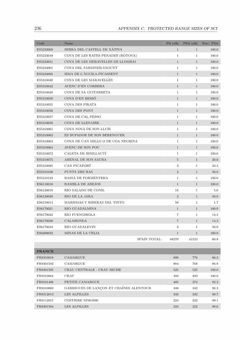
236 APPENDIX C. PROTECTED RANGE SIZES OF SCI
Code Name PA cells PSA cells Perc. PSA
ES5232009 SERRA DEL CASTELL DE XATIVA 1 1 100.0
ES5233049 COVA DE LES RATES PENADES (ROTOVA) 1 1 100.0
ES5233051 COVA DE LES MERAVELLES DE LLOMBAI 1 1 100.0
ES5234001 COVA DEL SARDINER-SAGUNT 1 1 100.0
ES5234005 SIMA DE L’AGUILA-PICASSENT 1 1 100.0
ES5310040 COVA DE LES MARAVELLES 1 1 100.0
ES5310042 AVENC D’EN CORBERA 1 1 100.0
ES5310048 COVA DE SA GUITARRETA 1 1 100.0
ES5310050 COVA D’EN BESSO 1 1 100.0
ES5310055 COVA DES PIRATA 1 1 100.0
ES5310056 COVA DES PONT 1 1 100.0
ES5310057 COVA DE CAL PESSO 1 1 100.0
ES5310059 COVA DE LLENAIRE 1 1 100.0
ES5310061 COVA NOVA DE SON LLUIS 1 1 100.0
ES5310062 ES BUFADOR DE SON BERENGUER 1 1 100.0
ES5310063 COVA DE CAN MILLO O DE COA NEGRINA 1 1 100.0
ES5310064 AVENC DE SON POU 1 1 100.0
ES5310072 CALETA DE BINILLAUTI 1 1 100.0
ES5310075 ARENAL DE SON SAURA 5 1 20.0
ES5310095 CAN PICAFORT 3 1 33.3
ES5310100 PUNTA DES RAS 2 1 50.0
ES5310123 BASSA DE FORMENTERA 1 1 100.0
ES6110016 RAMBLA DE AREJOS 1 1 100.0
ES6120019 RIO SALADO DE CONIL 18 1 5.6
ES6120028 RIO DE LA JARA 2 1 50.0
ES6150014 MARISMAS Y RIBERAS DEL TINTO 59 1 1.7
ES6170021 RIO GUADALMINA 1 1 100.0
ES6170022 RIO FUENGIROLA 7 1 14.3
ES6170030 CALAHONDA 7 1 14.3
ES6170034 RIO GUADALEVIN 2 1 50.0
ES6200032 MINAS DE LA CELIA 1 1 100.0
SPAIN TOTAL: 68270 41523 60.8
FRANCE
FR9310019 CAMARGUE 899 776 86.3
FR9301592 CAMARGUE 884 768 86.9
FR9301595 CRAU CENTRALE - CRAU SECHE 525 525 100.0
FR9310064 CRAU 493 493 100.0
FR9101406 PETITE CAMARGUE 405 374 92.3
FR9310069 GARRIGUES DE LANCON ET CHAINES ALENTOUR 348 342 98.3
FR9312013 LES ALPILLES 333 332 99.7
FR9112015 COSTIERE NIMOISE 224 222 99.1
FR9301594 LES ALPILLES 223 222 99.6

237
Code Name PA cells PSA cells Perc. PSA
FR9301596 MARAIS DE LA VALLEE DES BAUX ET MARAIS D’ARLES 189 189 100.0
FR9112013 PETITE CAMARGUE LAGUNO-MARINE 208 186 89.4
FR9301589 LA DURANCE 413 153 37.0
FR9312003 LA DURANCE 450 153 34.0
FR9301590 LE RHONE AVAL 318 141 44.3
FR9400574 PORTO/SCANDOLA/REVELLATA/CALVI/CALANCHES
DE PIANA (ZONE TERRESTRE ET MARINE)
202 135 66.8
FR9112007 ETANGS DU NARBONNAIS 142 122 85.9
FR9410023 GOLFE DE PORTO ET PRESQU’ILE DE SCANDOLA 181 118 65.2
FR9301603 CHAINE DE L’ETOILE- MASSIF DU GARLABAN 139 116 83.5
FR9312001 MARAIS ENTRE CRAU ET GRAND RHONE 110 110 100.0
FR9112004 HAUTES GARRIGUES DU MONTPELLIERAIS 553 107 19.3
FR9400570 AGRIATES 151 105 69.5
FR9110080 MONTAGNE DE LA CLAPE 120 104 86.7
FR9101453 MASSIF DE LA CLAPE 113 103 91.2
FR9112018 ETANG DE THAU ET LIDO DE SETE A AGDE 110 98 89.1
FR9101440 COMPLEXE LAGUNAIRE DE BAGES-SIGEAN 106 93 87.7
FR9101408 ETANG DE MAUGUIO 102 90 88.2
FR9112001 CAMARGUE GARDOISE FLUVIO-LACUSTRE 90 90 100.0
FR9112017 ETANG DE MAUGUIO 102 90 88.2
FR9112022 EST ET SUD DE BEZIERS 94 84 89.4
FR9101463 COMPLEXE LAGUNAIRE DE SALSES 89 82 92.1
FR9112005 COMPLEXE LAGUNAIRE DE SALSES-LEUCATE 85 79 92.9
FR9101393 MONTAGNE DE LA MOURE ET CAUSSE D’AUMELAS 137 77 56.2
FR9112021 PLAINE DE VILLEVEYRAC-MONTAGNAC 74 74 100.0
FR9101410 ETANGS PALAVASIENS 100 73 73.0
FR9110042 ETANGS PALAVASIENS ET ETANG DE L’ESTAGNOL 100 73 73.0
FR9101405 LE PETIT RHONE 73 72 98.6
FR9312009 PLATEAU DE L’ARBOIS 68 68 100.0
FR9301601 COTE BLEUE - CHAINE DE L’ESTAQUE 84 67 79.8
FR9110108 BASSE PLAINE DE L’AUDE 72 63 87.5
FR9101411 HERBIERS DE L’ETANG DE THAU 67 59 88.1
FR9112020 PLAINE DE FABREGUES-POUSSAN 51 51 100.0
FR9301622 LA PLAINE ET LE MASSIF DES MAURES 450 51 11.3
FR9301578 LA SORGUES ET L’AUZON 97 50 51.5
FR9301613 RADE D’HYERES 141 48 34.0
FR9101439 COLLINES DU NARBONNAIS 45 45 100.0
FR9112006 ETANG DE LAPALME 55 45 81.8
FR9400568 CAP CORSE NORD ET ILE FINOCCHIAROLA, GIRAGLIA
ET CAPENSE (COTE DE MACINAGGIO A C
47 44 93.6
FR9101435 BASSE PLAINE DE L’AUDE 47 42 89.4
FR9101436 COURS INFERIEUR DE L’AUDE 43 41 95.3
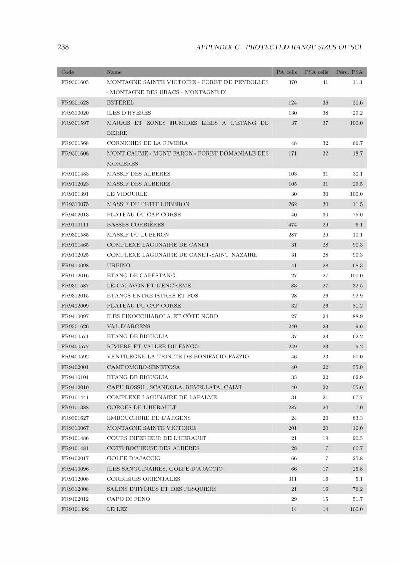
238 APPENDIX C. PROTECTED RANGE SIZES OF SCI
Code Name PA cells PSA cells Perc. PSA
FR9301605 MONTAGNE SAINTE VICTOIRE - FORET DE PEYROLLES
- MONTAGNE DES UBACS - MONTAGNE D’
370 41 11.1
FR9301628 ESTEREL 124 38 30.6
FR9310020 ILES D’HYERES 130 38 29.2
FR9301597 MARAIS ET ZONES HUMIDES LIEES A L’ETANG DE
BERRE
37 37 100.0
FR9301568 CORNICHES DE LA RIVIERA 48 32 66.7
FR9301608 MONT CAUME - MONT FARON - FORET DOMANIALE DES
MORIERES
171 32 18.7
FR9101483 MASSIF DES ALBERES 103 31 30.1
FR9112023 MASSIF DES ALBERES 105 31 29.5
FR9101391 LE VIDOURLE 30 30 100.0
FR9310075 MASSIF DU PETIT LUBERON 262 30 11.5
FR9402013 PLATEAU DU CAP CORSE 40 30 75.0
FR9110111 BASSES CORBIERES 474 29 6.1
FR9301585 MASSIF DU LUBERON 287 29 10.1
FR9101465 COMPLEXE LAGUNAIRE DE CANET 31 28 90.3
FR9112025 COMPLEXE LAGUNAIRE DE CANET-SAINT NAZAIRE 31 28 90.3
FR9410098 URBINO 41 28 68.3
FR9112016 ETANG DE CAPESTANG 27 27 100.0
FR9301587 LE CALAVON ET L’ENCREME 83 27 32.5
FR9312015 ETANGS ENTRE ISTRES ET FOS 28 26 92.9
FR9412009 PLATEAU DU CAP CORSE 32 26 81.2
FR9410097 ILES FINOCCHIAROLA ET COTE NORD 27 24 88.9
FR9301626 VAL D’ARGENS 240 23 9.6
FR9400571 ETANG DE BIGUGLIA 37 23 62.2
FR9400577 RIVIERE ET VALLEE DU FANGO 249 23 9.2
FR9400592 VENTILEGNE-LA TRINITE DE BONIFACIO-FAZZIO 46 23 50.0
FR9402001 CAMPOMORO-SENETOSA 40 22 55.0
FR9410101 ETANG DE BIGUGLIA 35 22 62.9
FR9412010 CAPU ROSSU , SCANDOLA, REVELLATA, CALVI 40 22 55.0
FR9101441 COMPLEXE LAGUNAIRE DE LAPALME 31 21 67.7
FR9101388 GORGES DE L’HERAULT 287 20 7.0
FR9301627 EMBOUCHURE DE L’ARGENS 24 20 83.3
FR9310067 MONTAGNE SAINTE VICTOIRE 201 20 10.0
FR9101486 COURS INFERIEUR DE L’HERAULT 21 19 90.5
FR9101481 COTE ROCHEUSE DES ALBERES 28 17 60.7
FR9402017 GOLFE D’AJACCIO 66 17 25.8
FR9410096 ILES SANGUINAIRES, GOLFE D’AJACCIO 66 17 25.8
FR9112008 CORBIERES ORIENTALES 311 16 5.1
FR9312008 SALINS D’HYERES ET DES PESQUIERS 21 16 76.2
FR9402012 CAPO DI FENO 29 15 51.7
FR9101392 LE LEZ 14 14 100.0

239
Code Name PA cells PSA cells Perc. PSA
FR9402018 CAP ROSSU, SCANDOLA, POINTE DE LA REVELETTA,
CANYON DE CALVI
25 14 56.0
FR9412007 VALLEE DU REGINO 56 14 25.0
FR9312005 SALINES DE L’ETANG DE BERRE 11 11 100.0
FR9400580 MARAIS DEL SALE, ZONES HUMIDES PERIPHERIQUES ET
FORET LITTORALE DE PINIA
22 11 50.0
FR9400593 ROCCAPINA-ORTOLO 24 11 45.8
FR9402015 BOUCHES DE BONIFACIO, ILES DES MOINES 87 11 12.6
FR9410021 ILES LAVEZZI, BOUCHES DE BONIFACIO 111 11 9.9
FR9101412 ETANG DU BAGNAS 13 10 76.9
FR9101478 LE TECH 79 10 12.7
FR9110034 ETANG DU BAGNAS 12 10 83.3
FR9301610 CAP SICIE - SIX FOURS 18 10 55.6
FR9101493 EMBOUCHURE DU TECH ET GRAU DE LA MASSANE 14 8 57.1
FR9102005 AQUEDUC DE PEZENAS 8 8 100.0
FR9112034 CAP BEAR- CAP CERBERE 16 8 50.0
FR9312014 COLLE DU ROUET 151 8 5.3
FR9400572 MUCCHIATANA 9 8 88.9
FR9400601 ALISO-OLETTA 9 8 88.9
FR9112002 LE SALAGOU 173 7 4.0
FR9301567 VALLEE DU CARAI - COLLINES DE CASTILLON 73 7 9.6
FR9301571 RIVIERE ET GORGES DU LOUP 84 7 8.3
FR9301609 LA POINTE FAUCONNIERE 11 7 63.6
FR9301624 CORNICHE VAROISE 34 7 20.6
FR9312002 PREALPES DE GRASSE 312 7 2.2
FR9312018 FALAISES DE VAUFREGES 7 7 100.0
FR9400602 BASSE VALLEE DU TAVIGNANO 55 7 12.7
FR9402016 POINTE DE SENETOSA ET PROLONGEMENTS 35 7 20.0
FR9101442 PLATEAU DE LEUCATE 9 6 66.7
FR9301572 DOME DE BIOT 6 6 100.0
FR9400588 SUBERAIE DE CECCIA/PORTO-VECCHIO 28 6 21.4
FR9400599 STRETTES DE ST FLORENT 6 6 100.0
FR9112030 PLATEAU DE LEUCATE 8 5 62.5
FR9400590 TRE PADULE DE SUARTONE, RONDINARA 11 5 45.5
FR9101389 PIC SAINT-LOUP 71 4 5.6
FR9101430 PLATEAU DE ROQUEHAUTE 4 4 100.0
FR9101433 LA GRANDE MAIRE 9 4 44.4
FR9102001 FRICHES HUMIDES DE TORREMILLA 4 4 100.0
FR9112035 COTE LANGUEDOCIENNE 44 4 9.1
FR9301998 BAIE DE LA CIOTAT 10 4 40.0
FR9312025 BASSE VALLEE DU VAR 31 4 12.9
FR9400586 EMBOUCHURE DU STABIACCU, DOMAINE PUBLIC MAR-
ITIME ET ILOT ZIGLIONE
6 4 66.7
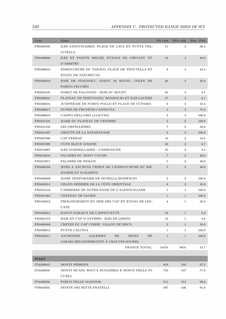
240 APPENDIX C. PROTECTED RANGE SIZES OF SCI
Code Name PA cells PSA cells Perc. PSA
FR9400595 ILES SANGUINAIRES, PLAGE DE LAVA ET PUNTA PEL-
LUSELLA
11 4 36.4
FR9400609 ILES ET POINTE BRUZZI, ETANGS DE CHEVANU ET
D’ARBITRU
10 4 40.0
FR9400610 EMBOUCHURE DU TARAVO, PLAGE DE TENUTELLA ET
ETANG DE TANCHICCIA
9 4 44.4
FR9402010 BAIE DE STAGNOLU, GOLFU DI SOGNU, GOLFE DE
PORTO-VECCHIO
20 4 20.0
FR9301625 FORET DE PALAYSON - BOIS DU ROUET 82 3 3.7
FR9400591 PLATEAU DE PERTUSATO/ BONIFACIO ET ILES LAVEZZI 37 3 8.1
FR9400616 JUNIPERAIE DE PORTO POLLO ET PLAGE DE CUPABIA 9 3 33.3
FR9400617 DUNES DE PRUNETE-CANNICCIA 4 3 75.0
FR9400619 CAMPO DELL’ORO (AJACCIO) 3 3 100.0
FR9101431 MARE DU PLATEAU DE VENDRES 2 2 100.0
FR9101434 LES ORPELLIERES 7 2 28.6
FR9101487 GROTTE DE LA RATAPANADE 2 2 100.0
FR9301996 CAP FERRAT 19 2 10.5
FR9301999 COTE BLEUE MARINE 30 2 6.7
FR9312007 ILES MARSEILLAISES - CASSIDAIGNE 45 2 4.4
FR9312016 FALAISES DU MONT CAUME 7 2 28.6
FR9312017 FALAISES DE NIOLON 5 2 40.0
FR9400594 SITES A ANCHUSA CRISPA DE L’EMBOUCHURE DU RIZ-
ZANESE ET D’OLMETO
5 2 40.0
FR9402009 MARE TEMPORAIRE DE MUSELLA/BONIFACIO 2 2 100.0
FR9402014 GRAND HERBIER DE LA COTE ORIENTALE 8 2 25.0
FR9101416 CARRIERES DE NOTRE-DAME DE L’AGENOUILLADE 1 1 100.0
FR9101464 CHATEAU DE SALSES 1 1 100.0
FR9102012 PROLONGEMENT EN MER DES CAP ET ETANG DE LEU-
CATE
4 1 25.0
FR9102014 BANCS SABLEUX DE L’ESPIGUETTE 16 1 6.2
FR9301573 BAIE ET CAP D’ANTIBES - ILES DE LERINS 18 1 5.6
FR9400569 CRETES DU CAP CORSE, VALLON DE SISCO 2 1 50.0
FR9400612 PUNTA CALCINA 1 1 100.0
FR9402011 ANCIENNES GALERIES DE MINES DE
LOZARI/BELGODERE(SITE A CHAUVES-SOURIS)
1 1 100.0
FRANCE TOTAL: 16476 9018 54.7
ITALY
ITA030043 MONTI NEBRODI 819 553 67.5
ITA020048 MONTI SICANI, ROCCA BUSAMBRA E BOSCO DELLA FI-
CUZZA
750 537 71.6
ITA020050 PARCO DELLE MADONIE 514 512 99.6
ITB043055 MONTE DEI SETTE FRATELLI 487 446 91.6
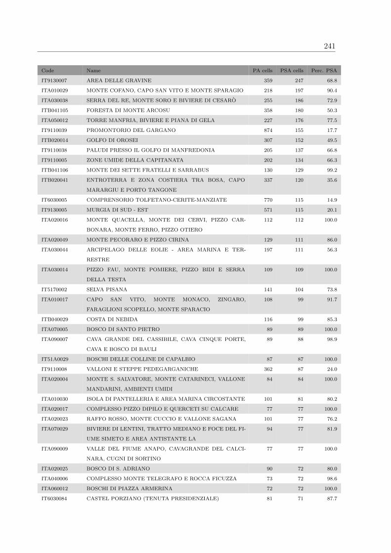
241
Code Name PA cells PSA cells Perc. PSA
IT9130007 AREA DELLE GRAVINE 359 247 68.8
ITA010029 MONTE COFANO, CAPO SAN VITO E MONTE SPARAGIO 218 197 90.4
ITA030038 SERRA DEL RE, MONTE SORO E BIVIERE DI CESARO 255 186 72.9
ITB041105 FORESTA DI MONTE ARCOSU 358 180 50.3
ITA050012 TORRE MANFRIA, BIVIERE E PIANA DI GELA 227 176 77.5
IT9110039 PROMONTORIO DEL GARGANO 874 155 17.7
ITB020014 GOLFO DI OROSEI 307 152 49.5
IT9110038 PALUDI PRESSO IL GOLFO DI MANFREDONIA 205 137 66.8
IT9110005 ZONE UMIDE DELLA CAPITANATA 202 134 66.3
ITB041106 MONTE DEI SETTE FRATELLI E SARRABUS 130 129 99.2
ITB020041 ENTROTERRA E ZONA COSTIERA TRA BOSA, CAPO
MARARGIU E PORTO TANGONE
337 120 35.6
IT6030005 COMPRENSORIO TOLFETANO-CERITE-MANZIATE 770 115 14.9
IT9130005 MURGIA DI SUD - EST 571 115 20.1
ITA020016 MONTE QUACELLA, MONTE DEI CERVI, PIZZO CAR-
BONARA, MONTE FERRO, PIZZO OTIERO
112 112 100.0
ITA020049 MONTE PECORARO E PIZZO CIRINA 129 111 86.0
ITA030044 ARCIPELAGO DELLE EOLIE - AREA MARINA E TER-
RESTRE
197 111 56.3
ITA030014 PIZZO FAU, MONTE POMIERE, PIZZO BIDI E SERRA
DELLA TESTA
109 109 100.0
IT5170002 SELVA PISANA 141 104 73.8
ITA010017 CAPO SAN VITO, MONTE MONACO, ZINGARO,
FARAGLIONI SCOPELLO, MONTE SPARACIO
108 99 91.7
ITB040029 COSTA DI NEBIDA 116 99 85.3
ITA070005 BOSCO DI SANTO PIETRO 89 89 100.0
ITA090007 CAVA GRANDE DEL CASSIBILE, CAVA CINQUE PORTE,
CAVA E BOSCO DI BAULI
89 88 98.9
IT51A0029 BOSCHI DELLE COLLINE DI CAPALBIO 87 87 100.0
IT9110008 VALLONI E STEPPE PEDEGARGANICHE 362 87 24.0
ITA020004 MONTE S. SALVATORE, MONTE CATARINECI, VALLONE
MANDARINI, AMBIENTI UMIDI
84 84 100.0
ITA010030 ISOLA DI PANTELLERIA E AREA MARINA CIRCOSTANTE 101 81 80.2
ITA020017 COMPLESSO PIZZO DIPILO E QUERCETI SU CALCARE 77 77 100.0
ITA020023 RAFFO ROSSO, MONTE CUCCIO E VALLONE SAGANA 101 77 76.2
ITA070029 BIVIERE DI LENTINI, TRATTO MEDIANO E FOCE DEL FI-
UME SIMETO E AREA ANTISTANTE LA
94 77 81.9
ITA090009 VALLE DEL FIUME ANAPO, CAVAGRANDE DEL CALCI-
NARA, CUGNI DI SORTINO
77 77 100.0
ITA020025 BOSCO DI S. ADRIANO 90 72 80.0
ITA040006 COMPLESSO MONTE TELEGRAFO E ROCCA FICUZZA 73 72 98.6
ITA060012 BOSCHI DI PIAZZA ARMERINA 72 72 100.0
IT6030084 CASTEL PORZIANO (TENUTA PRESIDENZIALE) 81 71 87.7
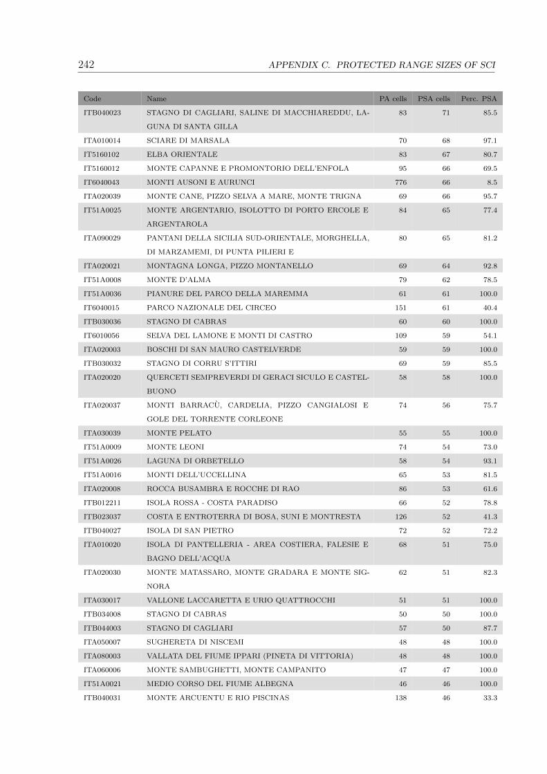
242 APPENDIX C. PROTECTED RANGE SIZES OF SCI
Code Name PA cells PSA cells Perc. PSA
ITB040023 STAGNO DI CAGLIARI, SALINE DI MACCHIAREDDU, LA-
GUNA DI SANTA GILLA
83 71 85.5
ITA010014 SCIARE DI MARSALA 70 68 97.1
IT5160102 ELBA ORIENTALE 83 67 80.7
IT5160012 MONTE CAPANNE E PROMONTORIO DELL’ENFOLA 95 66 69.5
IT6040043 MONTI AUSONI E AURUNCI 776 66 8.5
ITA020039 MONTE CANE, PIZZO SELVA A MARE, MONTE TRIGNA 69 66 95.7
IT51A0025 MONTE ARGENTARIO, ISOLOTTO DI PORTO ERCOLE E
ARGENTAROLA
84 65 77.4
ITA090029 PANTANI DELLA SICILIA SUD-ORIENTALE, MORGHELLA,
DI MARZAMEMI, DI PUNTA PILIERI E
80 65 81.2
ITA020021 MONTAGNA LONGA, PIZZO MONTANELLO 69 64 92.8
IT51A0008 MONTE D’ALMA 79 62 78.5
IT51A0036 PIANURE DEL PARCO DELLA MAREMMA 61 61 100.0
IT6040015 PARCO NAZIONALE DEL CIRCEO 151 61 40.4
ITB030036 STAGNO DI CABRAS 60 60 100.0
IT6010056 SELVA DEL LAMONE E MONTI DI CASTRO 109 59 54.1
ITA020003 BOSCHI DI SAN MAURO CASTELVERDE 59 59 100.0
ITB030032 STAGNO DI CORRU S’ITTIRI 69 59 85.5
ITA020020 QUERCETI SEMPREVERDI DI GERACI SICULO E CASTEL-
BUONO
58 58 100.0
ITA020037 MONTI BARRACU, CARDELIA, PIZZO CANGIALOSI E
GOLE DEL TORRENTE CORLEONE
74 56 75.7
ITA030039 MONTE PELATO 55 55 100.0
IT51A0009 MONTE LEONI 74 54 73.0
IT51A0026 LAGUNA DI ORBETELLO 58 54 93.1
IT51A0016 MONTI DELL’UCCELLINA 65 53 81.5
ITA020008 ROCCA BUSAMBRA E ROCCHE DI RAO 86 53 61.6
ITB012211 ISOLA ROSSA - COSTA PARADISO 66 52 78.8
ITB023037 COSTA E ENTROTERRA DI BOSA, SUNI E MONTRESTA 126 52 41.3
ITB040027 ISOLA DI SAN PIETRO 72 52 72.2
ITA010020 ISOLA DI PANTELLERIA - AREA COSTIERA, FALESIE E
BAGNO DELL’ACQUA
68 51 75.0
ITA020030 MONTE MATASSARO, MONTE GRADARA E MONTE SIG-
NORA
62 51 82.3
ITA030017 VALLONE LACCARETTA E URIO QUATTROCCHI 51 51 100.0
ITB034008 STAGNO DI CABRAS 50 50 100.0
ITB044003 STAGNO DI CAGLIARI 57 50 87.7
ITA050007 SUGHERETA DI NISCEMI 48 48 100.0
ITA080003 VALLATA DEL FIUME IPPARI (PINETA DI VITTORIA) 48 48 100.0
ITA060006 MONTE SAMBUGHETTI, MONTE CAMPANITO 47 47 100.0
IT51A0021 MEDIO CORSO DEL FIUME ALBEGNA 46 46 100.0
ITB040031 MONTE ARCUENTU E RIO PISCINAS 138 46 33.3

243
Code Name PA cells PSA cells Perc. PSA
IT9310304 ALTO IONIO COSENTINO 381 45 11.8
ITA010019 ISOLA DI PANTELLERIA: MONTAGNA GRANDE E MONTE
GIBELE
45 45 100.0
ITA020031 MONTE D’INDISI, MONTAGNA DEI CAVALLI, PIZZO PON-
TORNO E PIAN DEL LEONE
48 45 93.8
ITA090020 MONTI CLIMITI 45 45 100.0
ITA020002 BOSCHI DI GIBILMANNA E CEFALU 44 44 100.0
IT9350300 COSTA VIOLA 239 43 18.0
ITA020007 BOSCHI FICUZZA E CAPPELLIERE, VALLONE CERASA,
CASTAGNETI MEZZOJUSO
59 43 72.9
ITA050001 BIVIERE E MACCONI DI GELA 55 43 78.2
ITA010031 LAGHETTI DI PREOLA E GORGHI TONDI, SCIARE DI
MAZARA E PANTANO LEONE
42 42 100.0
ITA020028 SERRA DEL LEONE E MONTE STAGNATARO 51 42 82.4
ITA040007 PIZZO DELLA RONDINE, BOSCO DI S. STEFANO
QUISQUINA
48 42 87.5
IT6010017 SISTEMA FLUVIALE FIORA - OLPETA 57 41 71.9
IT9110012 TESTA DEL GARGANO 97 41 42.3
ITA010015 COMPLESSO MONTI DI CASTELLAMMARE DEL GOLFO
(TP)
44 41 93.2
ITA020018 FOCE DEL FIUME POLLINA E MONTE TARDARA 41 41 100.0
ITA010005 LAGHETTI DI PREOLA E GORGHI TONDI E SCIARE DI
MAZARA
40 40 100.0
ITA020033 MONTE SAN CALOGERO (TERMINI IMERESE) 40 40 100.0
ITB022212 SUPRAMONTE DI OLIENA, ORGOSOLO E URZULEI - SU
SERCONE
281 40 14.2
ITA020026 MONTE PIZZUTA, COSTA DEL CARPINETO, MOARDA 40 39 97.5
ITA010027 ARCIPELAGO DELLE EGADI - AREA MARINA E TER-
RESTRE
77 38 49.4
ITA020036 MONTE TRIONA E MONTE COLOMBA 57 38 66.7
ITA060010 VALLONE ROSSOMANNO 38 38 100.0
ITA020029 MONTE ROSE E MONTE PERNICE 38 37 97.4
ITA070001 FOCE DEL FIUME SIMETO E LAGO GORNALUNGA 37 37 100.0
ITB010042 CAPO CACCIA (CON LE ISOLE FORADADA E PIANA) E
PUNTA DEL GIGLIO
75 37 49.3
ITA030018 PIZZO MICHELE 36 36 100.0
ITA090016 ALTO CORSO DEL FIUME ASINARO, CAVA PIRARO E
CAVA CAROSELLO
36 36 100.0
ITB040021 COSTA DI CAGLIARI 44 36 81.8
IT8030008 DORSALE DEI MONTI LATTARI 184 35 19.0
IT9150002 COSTA OTRANTO - SANTA MARIA DI LEUCA 74 35 47.3
ITA020032 BOSCHI DI GRANZA 35 35 100.0
ITA030030 ISOLA DI LIPARI 53 35 66.0

244 APPENDIX C. PROTECTED RANGE SIZES OF SCI
Code Name PA cells PSA cells Perc. PSA
ITA090021 CAVA CONTESSA - CUGNO LUPO 35 35 100.0
ITB020015 AREA DEL MONTE FERRU DI TERTENIA 41 35 85.4
IT51A0019 ALTO CORSO DEL FIUME FIORA 122 34 27.9
IT9110015 DUNA E LAGO DI LESINA - FOCE DEL FORTORE 148 34 23.0
ITA060009 BOSCO DI SPERLINGA, ALTO SALSO 34 34 100.0
ITB033036 COSTA DI CUGLIERI 41 34 82.9
ITB040071 DA PISCINAS A RIU SCIVU 39 34 87.2
IT9320302 MARCHESATO E FIUME NETO 809 33 4.1
ITA010028 STAGNONE DI MARSALA E SALINE DI TRAPANI - AREA
MARINA E TERRESTRE
55 33 60.0
ITA020027 MONTE IATO, KUMETA, MAGANOCE E PIZZO PARRINO 54 33 61.1
ITA020035 MONTE GENUARDO E SANTA MARIA DEL BOSCO 35 33 94.3
ITA030042 MONTI PELORITANI, DORSALE CURCURACI, ANTENNA-
MARE E AREA MARINA DELLO STRETTO DI
245 33 13.5
ITB040030 CAPO PECORA 55 32 58.2
ITA030013 ROCCHE DI ALCARA LI FUSI 34 31 91.2
ITB040025 PROMONTORIO, DUNE E ZONA UMIDA DI PORTO PINO 40 31 77.5
ITA090019 CAVA CARDINALE 30 30 100.0
ITB010004 FOCI DEL COGHINAS 38 30 78.9
ITB044009 FORESTA DI MONTE ARCOSU 45 30 66.7
ITA080002 ALTO CORSO DEL FIUME IRMINO 29 29 100.0
ITA090022 BOSCO PISANO 29 29 100.0
ITB043025 STAGNI DI COLOSTRAI 36 29 80.6
IT9130004 MAR PICCOLO 39 28 71.8
ITA040005 MONTE CAMMARATA - CONTRADA SALACI 31 28 90.3
ITA090023 MONTE LAURO 28 28 100.0
IT8050048 COSTA TRA PUNTA TRESINO E LE RIPE ROSSE 54 27 50.0
ITA020040 MONTE ZIMMARA (GANGI) 27 27 100.0
ITA090002 VENDICARI 30 27 90.0
ITB010001 ISOLA ASINARA 86 27 31.4
ITB010082 ISOLA DELL’ASINARA 91 27 29.7
ITA020044 MONTE GRIFONE 35 26 74.3
ITA060005 LAGO DI ANCIPA 26 26 100.0
ITA090003 PANTANI DELLA SICILIA SUD ORIENTALE 37 26 70.3
ITB040024 ISOLA ROSSA E CAPO TEULADA 48 26 54.2
IT1323201 FINALESE - CAPO NOLI 49 25 51.0
IT6010016 MONTI DI CASTRO 25 25 100.0
ITA080009 CAVA D’ISPICA 25 25 100.0
ITA090018 FIUME TELLESIMO 25 25 100.0
ITB010043 COSTE E ISOLETTE A NORD OVEST DELLA SARDEGNA 48 25 52.1
ITB041111 MONTE LINAS - MARGANAI 300 25 8.3
IT51A0023 ISOLA DEL GIGLIO 34 24 70.6
IT8030010 FONDALI MARINI DI ISCHIA, PROCIDA E VIVARA 69 24 34.8

245
Code Name PA cells PSA cells Perc. PSA
IT9110009 VALLONI DI MATTINATA - MONTE SACRO 97 24 24.7
ITA090024 COZZO OGLIASTRI 24 24 100.0
ITB040022 STAGNO DI MOLENTARGIUS E TERRITORI LIMITROFI 30 24 80.0
IT9120002 MURGIA DEI TRULLI 95 23 24.2
IT9130006 PINETE DELL’ARCO IONICO 67 23 34.3
ITB034004 CORRU S’ITTIRI, STAGNO DI S. GIOVANNI E MARCEDDI 26 23 88.5
IT51A0011 PADULE DI DIACCIA BOTRONA 24 22 91.7
ITA010023 MONTAGNA GRANDE DI SALEMI 24 22 91.7
ITA010024 FONDALI DELL’ISOLA DI FAVIGNANA 36 22 61.1
ITA030027 ISOLA DI VULCANO 33 22 66.7
ITB010006 MONTE RUSSU 39 22 56.4
IT6030025 MACCHIA GRANDE DI PONTE GALERIA 21 21 100.0
IT9110025 MANACORE DEL GARGANO 32 21 65.6
IT9150009 LITORALE DI UGENTO 27 21 77.8
ITA010004 ISOLA DI FAVIGNANA 33 21 63.6
ITA010007 SALINE DI TRAPANI 25 21 84.0
ITA020011 ROCCHE DI CASTRONUOVO, PIZZO LUPO, GURGHI DI S.
ANDREA
31 21 67.7
ITA020034 MONTE CARCACI, PIZZO COLOBRIA E AMBIENTI UMIDI 28 21 75.0
ITA040004 FOCE DEL FIUME VERDURA 28 21 75.0
ITA060003 LAGO DI POZZILLO 52 21 40.4
ITA060004 MONTE ALTESINA 23 21 91.3
ITA070015 CANALONE DEL TRIPODO 31 21 67.7
IT9110037 LAGHI DI LESINA E VARANO 212 20 9.4
ITA010010 MONTE SAN GIULIANO 20 20 100.0
ITB011155 LAGO DI BARATZ - PORTO FERRO 25 20 80.0
ITB043035 COSTA E ENTROTERRA TRA PUNTA CANNONI E PUNTA
DELLE OCHE - ISOLA DI SAN PIETRO
28 20 71.4
ITB044002 SALINE DI MOLENTARGIUS 24 20 83.3
ITA020024 ROCCHE DI CIMINNA 27 19 70.4
ITA040003 FOCE DEL MAGAZZOLO, FOCE DEL PLATANI, CAPO
BIANCO, TORRE SALSA
34 19 55.9
IT1331402 BEIGUA - MONTE DENTE - GARGASSA - PAVAGLIONE 220 18 8.2
IT5160006 ISOLA DI CAPRAIA 33 18 54.5
IT8030005 CORPO CENTRALE DELL’ISOLA DI ISCHIA 24 18 75.0
IT9130002 MASSERIA TORRE BIANCA 18 18 100.0
IT9150011 ALIMINI 36 18 50.0
IT9340091 ZONA COSTIERA FRA BRIATICO E NICOTERA 40 18 45.0
ITB010008 ARCIPELAGO LA MADDALENA 126 18 14.3
ITB030037 STAGNO DI SANTA GIUSTA 20 18 90.0
IT1324910 MONTE ACUTO - POGGIO GRANDE - RIO TORSERO 45 17 37.8
IT5160007 ISOLA DI CAPRAIA - AREA TERRESTRE E MARINA 32 17 53.1
IT7228221 FOCE TRIGNO - MARINA DI PETACCIATO 27 17 63.0

246 APPENDIX C. PROTECTED RANGE SIZES OF SCI
Code Name PA cells PSA cells Perc. PSA
ITA030016 PIZZO DELLA BATTAGLIA 17 17 100.0
ITA030029 ISOLA DI SALINA (STAGNO DI LINGUA) 20 17 85.0
ITA070016 VALLE DEL BOVE 45 17 37.8
IT8050047 COSTA TRA MARINA DI CAMEROTA E POLICASTRO
BUSSENTINO
52 16 30.8
ITA030015 VALLE DEL FIUME CARONIA, LAGO ZILIO 16 16 100.0
ITA060008 CONTRADA GIAMMAIANO 16 16 100.0
ITA090017 CAVA PALOMBIERI 16 16 100.0
ITB010003 STAGNO E GINEPRETO DI PLATAMONA 28 16 57.1
ITB032228 IS ARENAS 20 16 80.0
IT51A0010 POGGIO DI MOSCONA 15 15 100.0
IT6040010 LAGO DI FONDI 19 15 78.9
IT9110016 PINETA MARZINI 18 15 83.3
ITA020014 MONTE PELLEGRINO 15 15 100.0
ITA060011 CONTRADA CAPRARA 21 15 71.4
ITB030035 STAGNO DI SALE ’E PORCUS 15 15 100.0
IT5160013 ISOLA DI PIANOSA 21 14 66.7
IT5160016 ISOLA DI PIANOSA - AREA TERRESTRE E MARINA 22 14 63.6
IT8010015 MONTE MASSICO 56 14 25.0
IT9150027 PALUDE DEL CONTE, DUNE DI PUNTA PROSCIUTTO 14 14 100.0
IT9350158 COSTA VIOLA E MONTE S. ELIA 22 14 63.6
ITA010008 COMPLESSO MONTE BOSCO E SCORACE 14 14 100.0
ITA020006 CAPO GALLO 14 14 100.0
ITA030003 RUPI DI TAORMINA E MONTE VENERETTA 14 14 100.0
ITB013044 CAPO CACCIA 51 14 27.5
ITB020012 BERCHIDA E BIDDEROSA 37 14 37.8
ITB034007 STAGNO DI SALE E’ PORCUS 14 14 100.0
ITB040019 STAGNI DI COLOSTRAI E DELLE SALINE 19 14 73.7
ITB043056 GIARA DI SIDDI 20 14 70.0
IT1323203 ROCCA DEI CORVI - MAO - MORTOU 30 13 43.3
IT1324909 TORRENTE ARROSCIA E CENTA 15 13 86.7
IT6030047 BOSCO DI FOGLINO 13 13 100.0
IT6040014 FORESTA DEMANIALE DEL CIRCEO 47 13 27.7
IT8030018 LAGO DI PATRIA 14 13 92.9
IT8050010 FASCE LITORANEE A DESTRA E A SINISTRA DEL FIUME
SELE
24 13 54.2
ITA070004 TIMPA DI ACIREALE 13 13 100.0
ITA070014 MONTE BARACCA, CONTRADA GIARRITA 29 13 44.8
ITA090006 SALINE DI SIRACUSA E FIUME CIANE 13 13 100.0
ITA090015 TORRENTE SAPILLONE 13 13 100.0
ITB030034 STAGNO DI MISTRAS DI ORISTANO 25 13 52.0
IT5160014 ISOLA DI MONTECRISTO 20 12 60.0

247
Code Name PA cells PSA cells Perc. PSA
IT5160017 ISOLA DI MONTECRISTO E FORMICA DI MONTECRISTO
- AREA TERRESTRE E MARINA
20 12 60.0
IT6030044 MACCHIA DELLA SPADELLATA E FOSSO S. ANASTASIO 12 12 100.0
IT9110004 FORESTA UMBRA 255 12 4.7
IT9130001 TORRE COLIMENA 31 12 38.7
IT9320095 FOCE NETO 15 12 80.0
ITA010011 SISTEMA DUNALE CAPO GRANITOLA, PORTO PALO E
FOCE DEL BELICE
31 12 38.7
ITA020038 SUGHERETE DI CONTRADA SERRADAINO 12 12 100.0
ITA030026 ISOLE DI STROMBOLI E STROMBOLICCHIO 19 12 63.2
ITA040010 LITORALE DI PALMA DI MONTECHIARO 19 12 63.2
ITA050009 RUPE DI MARIANOPOLI 23 12 52.2
ITA080006 CAVA RANDELLO, PASSO MARINARO 12 12 100.0
ITB010002 STAGNO DI PILO E DI CASARACCIO 28 12 42.9
ITB013019 ISOLE DEL NORD - EST TRA CAPO CERASO E STAGNO
DI SAN TEODORO
67 12 17.9
ITB040017 STAGNI DI MURTAS E S’ACQUA DURCI 15 12 80.0
ITB040018 FOCE DEL FLUMENDOSA - SA PRAIA 13 12 92.3
IT1315806 MONTE NERO - MONTE BIGNONE 55 11 20.0
IT5160009 PROMONTORIO DI PIOMBINO E MONTE MASSONCELLO 16 11 68.8
IT6030053 SUGHERETA DI CASTEL DI DECIMA 11 11 100.0
IT6040017 PROMONTORIO DEL CIRCEO (QUARTO FREDDO) 14 11 78.6
IT7222217 FOCE SACCIONE - BONIFICA RAMITELLI 20 11 55.0
IT8030011 FONDALI MARINI DI PUNTA CAMPANELLA E CAPRI 69 11 15.9
IT9120011 VALLE OFANTO - LAGO DI CAPACIOTTI 192 11 5.7
IT9150015 LITORALE DI GALLIPOLI E ISOLA S. ANDREA 18 11 61.1
IT9150030 BOSCO LA LIZZA E MACCHIA DEL PAGLIARONE 11 11 100.0
IT9310043 FIUMARA AVENA 22 11 50.0
IT9320104 COLLINE DI CROTONE 12 11 91.7
ITA010002 ISOLA DI MARETTIMO 24 11 45.8
ITA050011 TORRE MANFRIA 24 11 45.8
ITA060002 LAGO DI PERGUSA 11 11 100.0
ITA060013 SERRE DI MONTE CANNARELLA 25 11 44.0
ITB013012 STAGNO DI PILO, CASARACCIO E SALINE DI STINTINO 24 11 45.8
ITB040020 ISOLA DEI CAVOLI, SERPENTARA, PUNTA MOLENTIS E
CAMPULONGU
34 11 32.4
ITB042247 IS COMPINXIUS - CAMPO DUNALE DI BUGERRU - POR-
TIXEDDU
11 11 100.0
ITB043032 ISOLA DI SANT’ANTIOCO, CAPO SPERONE 23 11 47.8
IT5160003 TOMBOLO DI CECINA 19 10 52.6
IT5160004 PADULE DI BOLGHERI 10 10 100.0
IT51A0014 PINETA GRANDUCALE DELL’UCCELLINA 13 10 76.9
IT8050032 MONTE TRESINO E DINTORNI 22 10 45.5

248 APPENDIX C. PROTECTED RANGE SIZES OF SCI
Code Name PA cells PSA cells Perc. PSA
IT8050036 PARCO MARINO DI S. MARIA DI CASTELLABATE 21 10 47.6
IT9140002 LITORALE BRINDISINO 18 10 55.6
IT9310042 FIUMARA SARACENO 27 10 37.0
ITA060007 VALLONE DI PIANO DELLA CORTE 15 10 66.7
ITA060015 CONTRADA VALANGHE 39 10 25.6
ITA070018 PIANO DEI GRILLI 24 10 41.7
IT1315717 MONTE GRAMMONDO - TORRENTE BEVERA 45 9 20.0
IT1331578 BEIGUA - TURCHINO 145 9 6.2
IT1332603 PARCO DI PORTOFINO 25 9 36.0
IT6030004 VALLE DI RIO FIUME 26 9 34.6
IT6030028 CASTEL PORZIANO (QUERCETI IGROFILI) 9 9 100.0
IT8050026 MONTE LICOSA E DINTORNI 20 9 45.0
IT9150032 LE CESINE 19 9 47.4
IT9150033 SPECCHIA DELL’ALTO 14 9 64.3
IT9220055 BOSCO PANTANO DI POLICORO E COSTA IONICA FOCE
SINNI
23 9 39.1
ITA010021 SALINE DI MARSALA 14 9 64.3
ITA020019 RUPI DI CATALFANO E CAPO ZAFFERANO 10 9 90.0
ITA020022 CALANCHI, LEMBI BOSCHIVI E PRATERIE DI RIENA 16 9 56.2
ITA020047 FONDALI DI ISOLA DELLE FEMMINE - CAPO GALLO 12 9 75.0
ITB030016 STAGNO DI S’ENA ARRUBIA E TERRITORI LIMITROFI 9 9 100.0
ITB042226 STAGNO DI PORTO BOTTE 18 9 50.0
ITB043028 CAPO CARBONARA E STAGNO DI NOTTERI - PUNTA MO-
LENTIS
20 9 45.0
IT5120016 MACCHIA LUCCHESE 10 8 80.0
IT51A0012 TOMBOLO DA CASTIGLION DELLA PESCAIA A MARINA
DI GROSSETO
16 8 50.0
IT8030009 FOCE DI LICOLA 8 8 100.0
IT8050039 PINETA DI SANT’ICONIO 10 8 80.0
IT8050051 VALLONI DELLA COSTIERA AMALFITANA 15 8 53.3
IT9150006 RAUCCIO 12 8 66.7
IT9310044 FOCE DEL FIUME CRATI 10 8 80.0
IT9320106 STECCATO DI CUTRO E COSTA DEL TURCHESE 16 8 50.0
ITA010009 MONTE BONIFATO 8 8 100.0
ITA010016 MONTE COFANO E LITORALE 13 8 61.5
ITA020045 ROCCA DI SCIARA 8 8 100.0
ITA030024 ISOLA DI FILICUDI 15 8 53.3
ITA030028 ISOLA DI SALINA (MONTE FOSSA DELLE FELCI E DEI
PORRI)
15 8 53.3
ITB022214 LIDO DI ORRI 9 8 88.9
ITB034006 STAGNO DI MISTRAS 16 8 50.0
ITB042237 MONTE SAN MAURO 14 8 57.1
ITB042241 RIU S. BARZOLU 8 8 100.0

249
Code Name PA cells PSA cells Perc. PSA
ITB042250 DA IS ARENAS A TONNARA (MARINA DI GONNESA) 8 8 100.0
IT1315716 ROVERINO 9 7 77.8
IT1324007 MONTE CIAZZE SECCHE 9 7 77.8
IT1331718 MONTE FASCE 24 7 29.2
IT1333307 PUNTA BAFFE - PUNTA MONEGLIA - VAL PETRONIO 27 7 25.9
IT51A0013 PADULE DELLA TRAPPOLA, BOCCA D’OMBRONE 11 7 63.6
IT51A0030 LAGO ACQUATO, LAGO SAN FLORIANO 7 7 100.0
IT6010027 LITORALE TRA TARQUINIA E MONTALTO DI CASTRO 11 7 63.6
IT6010028 NECROPOLI DI TARQUINIA 7 7 100.0
IT6010039 ACROPOLI DI TARQUINIA 7 7 100.0
IT6040006 MONTI AUSONI MERIDIONALI 73 7 9.6
IT8050011 FASCIA INTERNA DI COSTA DEGLI INFRESCHI E DELLA
MASSETA
23 7 30.4
IT9140001 BOSCO TRAMAZZONE 9 7 77.8
IT9150007 TORRE ULUZZO 12 7 58.3
IT9150008 MONTAGNA SPACCATA E RUPI DI SAN MAURO 9 7 77.8
IT9310051 DUNE DI CAMIGLIANO 9 7 77.8
IT9350172 FONDALI DA PUNTA PEZZO A CAPO DELL’ARMI 22 7 31.8
ITA010006 PALUDI DI CAPO FETO E MARGI SPANO 15 7 46.7
ITA020009 CALA ROSSA E CAPO RAMA 13 7 53.8
ITA020043 MONTE ROSAMARINA E COZZO FAMO 7 7 100.0
ITA020046 FONDALI DELL’ISOLA DI USTICA 18 7 38.9
ITA030004 BACINO DEL TORRENTE LETOJANNI 25 7 28.0
ITA030022 LECCETA DI S. FRATELLO 7 7 100.0
ITA090008 CAPO MURRO DI PORCO, PENISOLA DELLA MAD-
DALENA E GROTTA PELLEGRINO
9 7 77.8
ITA090027 FONDALI DI VENDICARI 10 7 70.0
ITB020013 PALUDE DI OSALLA 23 7 30.4
ITB032219 SASSU - CIRRAS 7 7 100.0
ITB032229 IS ARENAS S’ACQUA E S’OLLASTU 7 7 100.0
ITB042234 MONTE MANNU - MONTE LADU (COLLINE DI MONTE
MANNU E MONTE LADU)
7 7 100.0
IT1345101 PIANA DEL MAGRA 17 6 35.3
IT51A0033 LAGO DI BURANO 12 6 50.0
IT6040016 PROMONTORIO DEL CIRCEO (QUARTO CALDO) 12 6 50.0
IT8010021 PINETA DI PATRIA 11 6 54.5
IT8010027 FIUMI VOLTURNO E CALORE BENEVENTANO 219 6 2.7
IT8010029 FIUME GARIGLIANO 46 6 13.0
IT8030006 COSTIERA AMALFITANA TRA NERANO E POSITANO 26 6 23.1
IT8030015 LAGO DEL FUSARO 6 6 100.0
IT9210160 ISOLA DI S. IANNI E COSTA PROSPICIENTE 9 6 66.7
ITA010001 ISOLE DELLO STAGNONE DI MARSALA 19 6 31.6
ITA010013 BOSCO DI CALATAFIMI 6 6 100.0
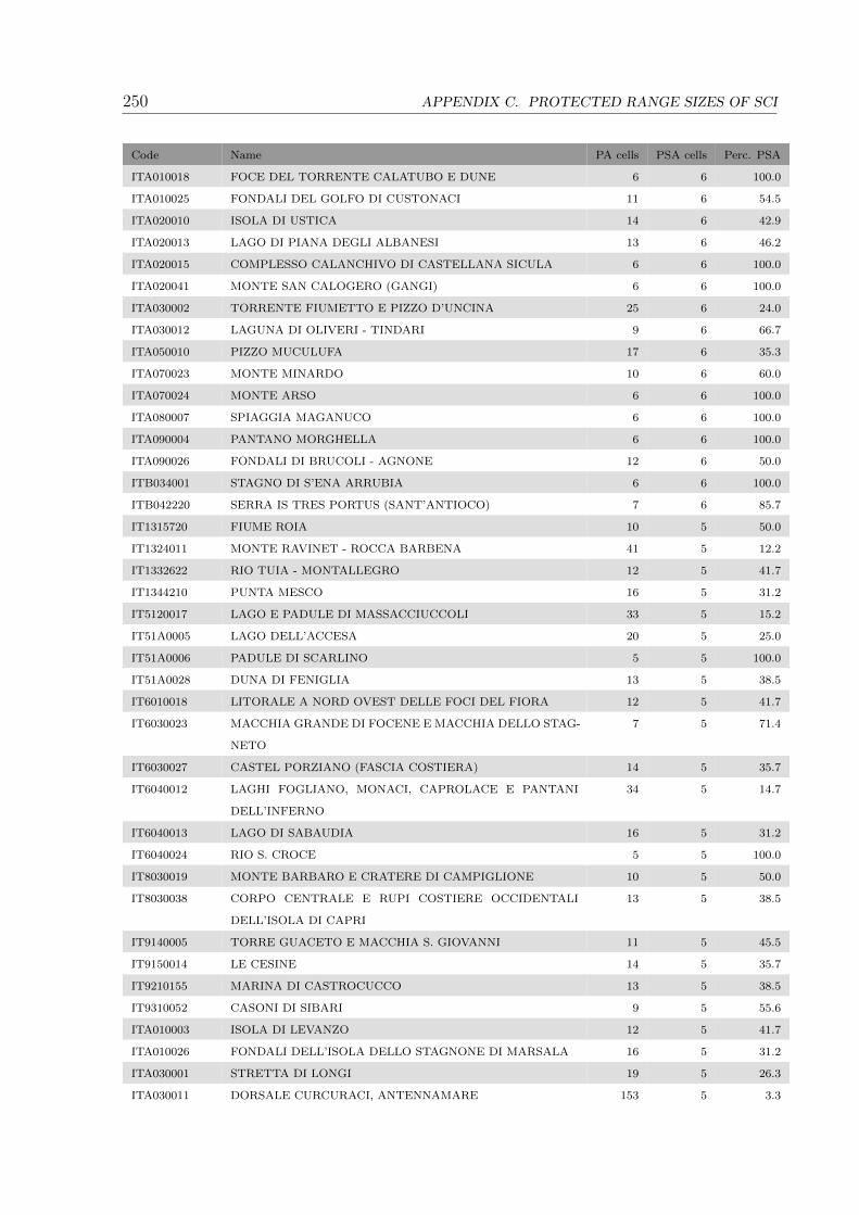
250 APPENDIX C. PROTECTED RANGE SIZES OF SCI
Code Name PA cells PSA cells Perc. PSA
ITA010018 FOCE DEL TORRENTE CALATUBO E DUNE 6 6 100.0
ITA010025 FONDALI DEL GOLFO DI CUSTONACI 11 6 54.5
ITA020010 ISOLA DI USTICA 14 6 42.9
ITA020013 LAGO DI PIANA DEGLI ALBANESI 13 6 46.2
ITA020015 COMPLESSO CALANCHIVO DI CASTELLANA SICULA 6 6 100.0
ITA020041 MONTE SAN CALOGERO (GANGI) 6 6 100.0
ITA030002 TORRENTE FIUMETTO E PIZZO D’UNCINA 25 6 24.0
ITA030012 LAGUNA DI OLIVERI - TINDARI 9 6 66.7
ITA050010 PIZZO MUCULUFA 17 6 35.3
ITA070023 MONTE MINARDO 10 6 60.0
ITA070024 MONTE ARSO 6 6 100.0
ITA080007 SPIAGGIA MAGANUCO 6 6 100.0
ITA090004 PANTANO MORGHELLA 6 6 100.0
ITA090026 FONDALI DI BRUCOLI - AGNONE 12 6 50.0
ITB034001 STAGNO DI S’ENA ARRUBIA 6 6 100.0
ITB042220 SERRA IS TRES PORTUS (SANT’ANTIOCO) 7 6 85.7
IT1315720 FIUME ROIA 10 5 50.0
IT1324011 MONTE RAVINET - ROCCA BARBENA 41 5 12.2
IT1332622 RIO TUIA - MONTALLEGRO 12 5 41.7
IT1344210 PUNTA MESCO 16 5 31.2
IT5120017 LAGO E PADULE DI MASSACCIUCCOLI 33 5 15.2
IT51A0005 LAGO DELL’ACCESA 20 5 25.0
IT51A0006 PADULE DI SCARLINO 5 5 100.0
IT51A0028 DUNA DI FENIGLIA 13 5 38.5
IT6010018 LITORALE A NORD OVEST DELLE FOCI DEL FIORA 12 5 41.7
IT6030023 MACCHIA GRANDE DI FOCENE E MACCHIA DELLO STAG-
NETO
7 5 71.4
IT6030027 CASTEL PORZIANO (FASCIA COSTIERA) 14 5 35.7
IT6040012 LAGHI FOGLIANO, MONACI, CAPROLACE E PANTANI
DELL’INFERNO
34 5 14.7
IT6040013 LAGO DI SABAUDIA 16 5 31.2
IT6040024 RIO S. CROCE 5 5 100.0
IT8030019 MONTE BARBARO E CRATERE DI CAMPIGLIONE 10 5 50.0
IT8030038 CORPO CENTRALE E RUPI COSTIERE OCCIDENTALI
DELL’ISOLA DI CAPRI
13 5 38.5
IT9140005 TORRE GUACETO E MACCHIA S. GIOVANNI 11 5 45.5
IT9150014 LE CESINE 14 5 35.7
IT9210155 MARINA DI CASTROCUCCO 13 5 38.5
IT9310052 CASONI DI SIBARI 9 5 55.6
ITA010003 ISOLA DI LEVANZO 12 5 41.7
ITA010026 FONDALI DELL’ISOLA DELLO STAGNONE DI MARSALA 16 5 31.2
ITA030001 STRETTA DI LONGI 19 5 26.3
ITA030011 DORSALE CURCURACI, ANTENNAMARE 153 5 3.3
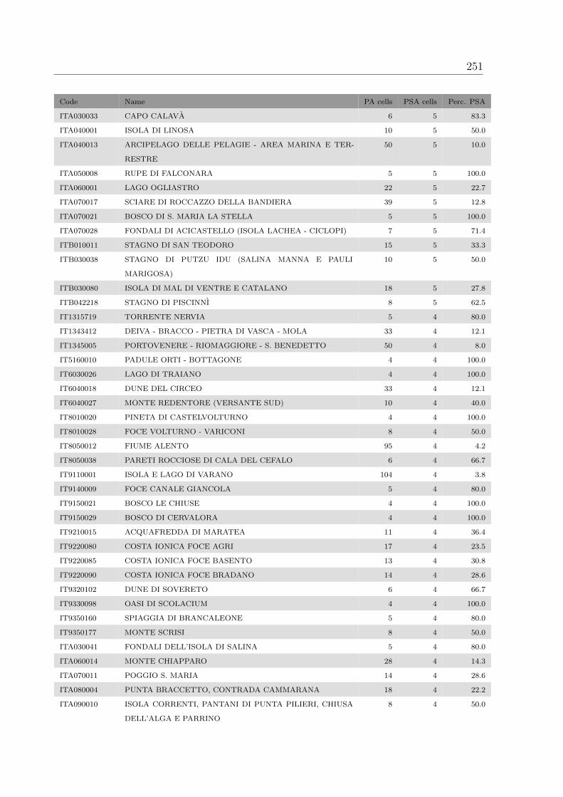
251
Code Name PA cells PSA cells Perc. PSA
ITA030033 CAPO CALAVA 6 5 83.3
ITA040001 ISOLA DI LINOSA 10 5 50.0
ITA040013 ARCIPELAGO DELLE PELAGIE - AREA MARINA E TER-
RESTRE
50 5 10.0
ITA050008 RUPE DI FALCONARA 5 5 100.0
ITA060001 LAGO OGLIASTRO 22 5 22.7
ITA070017 SCIARE DI ROCCAZZO DELLA BANDIERA 39 5 12.8
ITA070021 BOSCO DI S. MARIA LA STELLA 5 5 100.0
ITA070028 FONDALI DI ACICASTELLO (ISOLA LACHEA - CICLOPI) 7 5 71.4
ITB010011 STAGNO DI SAN TEODORO 15 5 33.3
ITB030038 STAGNO DI PUTZU IDU (SALINA MANNA E PAULI
MARIGOSA)
10 5 50.0
ITB030080 ISOLA DI MAL DI VENTRE E CATALANO 18 5 27.8
ITB042218 STAGNO DI PISCINNI 8 5 62.5
IT1315719 TORRENTE NERVIA 5 4 80.0
IT1343412 DEIVA - BRACCO - PIETRA DI VASCA - MOLA 33 4 12.1
IT1345005 PORTOVENERE - RIOMAGGIORE - S. BENEDETTO 50 4 8.0
IT5160010 PADULE ORTI - BOTTAGONE 4 4 100.0
IT6030026 LAGO DI TRAIANO 4 4 100.0
IT6040018 DUNE DEL CIRCEO 33 4 12.1
IT6040027 MONTE REDENTORE (VERSANTE SUD) 10 4 40.0
IT8010020 PINETA DI CASTELVOLTURNO 4 4 100.0
IT8010028 FOCE VOLTURNO - VARICONI 8 4 50.0
IT8050012 FIUME ALENTO 95 4 4.2
IT8050038 PARETI ROCCIOSE DI CALA DEL CEFALO 6 4 66.7
IT9110001 ISOLA E LAGO DI VARANO 104 4 3.8
IT9140009 FOCE CANALE GIANCOLA 5 4 80.0
IT9150021 BOSCO LE CHIUSE 4 4 100.0
IT9150029 BOSCO DI CERVALORA 4 4 100.0
IT9210015 ACQUAFREDDA DI MARATEA 11 4 36.4
IT9220080 COSTA IONICA FOCE AGRI 17 4 23.5
IT9220085 COSTA IONICA FOCE BASENTO 13 4 30.8
IT9220090 COSTA IONICA FOCE BRADANO 14 4 28.6
IT9320102 DUNE DI SOVERETO 6 4 66.7
IT9330098 OASI DI SCOLACIUM 4 4 100.0
IT9350160 SPIAGGIA DI BRANCALEONE 5 4 80.0
IT9350177 MONTE SCRISI 8 4 50.0
ITA030041 FONDALI DELL’ISOLA DI SALINA 5 4 80.0
ITA060014 MONTE CHIAPPARO 28 4 14.3
ITA070011 POGGIO S. MARIA 14 4 28.6
ITA080004 PUNTA BRACCETTO, CONTRADA CAMMARANA 18 4 22.2
ITA090010 ISOLA CORRENTI, PANTANI DI PUNTA PILIERI, CHIUSA
DELL’ALGA E PARRINO
8 4 50.0

252 APPENDIX C. PROTECTED RANGE SIZES OF SCI
Code Name PA cells PSA cells Perc. PSA
ITB040028 PUNTA S’ALIGA 11 4 36.4
ITB042223 STAGNO DI SANTA CATERINA 11 4 36.4
ITB042225 IS PRUINIS 6 4 66.7
IT1315922 POMPEIANA 6 3 50.0
IT1324896 LERRONE - VALLONI 5 3 60.0
IT1333308 PUNTA MANARA 6 3 50.0
IT1343419 MONTE SERRO 8 3 37.5
IT1343502 PARCO DELLA MAGRA - VARA 93 3 3.2
IT1344270 FONDALI PUNTA MESCO - RIO MAGGIORE 13 3 23.1
IT1344323 COSTA RIOMAGGIORE - MONTEROSSO 12 3 25.0
IT51A0004 POGGIO TRE CANCELLI 8 3 37.5
IT51A0015 DUNE COSTIERE DEL PARCO DELL’UCCELLINA 10 3 30.0
IT51A0024 ISOLA DI GIANNUTRI 10 3 30.0
IT51A0031 LAGO DI BURANO 7 3 42.9
IT51A0037 ISOLA DI GIANNUTRI - AREA TERRESTRE E MARINA 10 3 30.0
IT6010019 PIAN DEI CANGANI 4 3 75.0
IT6010026 SALINE DI TARQUINIA 6 3 50.0
IT6030016 ANTICA LAVINIUM - PRATICA DI MARE 3 3 100.0
IT6030019 MACCHIATONDA 6 3 50.0
IT6030045 LIDO DEI GIGLI 6 3 50.0
IT6040025 FIUME GARIGLIANO (TRATTO TERMINALE) 4 3 75.0
IT7222216 FOCE BIFERNO - LITORALE DI CAMPOMARINO 19 3 15.8
IT7228230 LAGO DI GUARDIALFIERA - FOCE FIUME BIFERNO 401 3 0.7
IT8010019 PINETA DELLA FOCE DEL GARIGLIANO 7 3 42.9
IT8030007 CRATERE DI ASTRONI 8 3 37.5
IT8030026 RUPI COSTIERE DELL’ISOLA DI ISCHIA 22 3 13.6
IT8050040 RUPI COSTIERE DELLA COSTA DEGLI INFRESCHI E
DELLA MASSETA
15 3 20.0
IT9140003 STAGNI E SALINE DI PUNTA DELLA CONTESSA 10 3 30.0
IT9140006 BOSCO DI SANTA TERESA 4 3 75.0
IT9140008 TORRE GUACETO 8 3 37.5
IT9150013 PALUDE DEL CAPITANO 4 3 75.0
IT9150024 TORRE INSERRAGLIO 5 3 60.0
IT9150025 TORRE VENERI 12 3 25.0
IT9310045 MACCHIA DELLA BURA 3 3 100.0
IT9330108 DUNE DI GUARDAVALLE 3 3 100.0
IT9330184 SCOGLIERA DI STALETTI 3 3 100.0
IT9350144 CALANCHI DI PALIZZI MARINA 5 3 60.0
IT9350148 FIUMARA DI PALIZZI 7 3 42.9
ITA010022 COMPLESSO MONTI DI SANTA NINFA - GIBELLINA E
GROTTA DI SANTA NINFA
14 3 21.4
ITA020001 ROCCA DI CEFALU 3 3 100.0
ITA020012 VALLE DEL FIUME ORETO 15 3 20.0
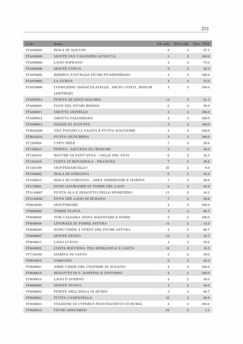
253
Code Name PA cells PSA cells Perc. PSA
ITA030023 ISOLA DI ALICUDI 8 3 37.5
ITA040009 MONTE SAN CALOGERO (SCIACCA) 3 3 100.0
ITA050003 LAGO SOPRANO 4 3 75.0
ITA050006 MONTE CONCA 9 3 33.3
ITA070002 RISERVA NATURALE FIUME FIUMEFREDDO 3 3 100.0
ITA070003 LA GURNA 4 3 75.0
ITA070008 COMPLESSO IMMACOLATELLE, MICIO CONTI, BOSCHI
LIMITROFI
3 3 100.0
ITA070013 PINETA DI LINGUAGLOSSA 14 3 21.4
ITA080001 FOCE DEL FIUME IRMINO 6 3 50.0
ITA090011 GROTTA MONELLO 3 3 100.0
ITA090012 GROTTA PALOMBARA 3 3 100.0
ITA090014 SALINE DI AUGUSTA 3 3 100.0
ITB042208 TRA POGGIO LA SALINA E PUNTA MAGGIORE 3 3 100.0
ITB042210 PUNTA GIUNCHERA 3 3 100.0
IT1325624 CAPO MELE 7 2 28.6
IT1332614 PINETA - LECCETA DI CHIAVARI 5 2 40.0
IT1333316 ROCCHE DI SANT’ANNA - VALLE DEL FICO 6 2 33.3
IT1344216 COSTA DI BONASSOLA - FRAMURA 7 2 28.6
IT1345109 MONTEMARCELLO 25 2 8.0
IT5160002 ISOLA DI GORGONA 6 2 33.3
IT5160015 ISOLA DI GORGONA - AREA TERRESTRE E MARINA 7 2 28.6
IT5170001 DUNE LITORANEE DI TORRE DEL LAGO 6 2 33.3
IT51A0007 PUNTA ALA E ISOLOTTO DELLO SPARVIERO 11 2 18.2
IT51A0032 DUNA DEL LAGO DI BURANO 7 2 28.6
IT6010040 MONTEROZZI 2 2 100.0
IT6030020 TORRE FLAVIA 3 2 66.7
IT6030046 TOR CALDARA (ZONA SOLFATARE E FOSSI) 2 2 100.0
IT6030048 LITORALE DI TORRE ASTURA 15 2 13.3
IT6030049 ZONE UMIDE A OVEST DEL FIUME ASTURA 3 2 66.7
IT6040007 MONTE LEANO 12 2 16.7
IT6040011 LAGO LUNGO 4 2 50.0
IT6040022 COSTA ROCCIOSA TRA SPERLONGA E GAETA 19 2 10.5
IT7140109 MARINA DI VASTO 4 2 50.0
IT8010018 VARICONI 6 2 33.3
IT8030001 AREE UMIDE DEL CRATERE DI AGNANO 2 2 100.0
IT8030013 ISOLOTTO DI S. MARTINO E DINTORNI 2 2 100.0
IT8030014 LAGO D’AVERNO 4 2 50.0
IT8030020 MONTE NUOVO 4 2 50.0
IT8030022 PINETE DELL’ISOLA DI ISCHIA 3 2 66.7
IT8030024 PUNTA CAMPANELLA 10 2 20.0
IT8030034 STAZIONE DI CYPERUS POLYSTACHYUS DI ISCHIA 2 2 100.0
IT8050013 FIUME MINGARDO 64 2 3.1

254 APPENDIX C. PROTECTED RANGE SIZES OF SCI
Code Name PA cells PSA cells Perc. PSA
IT8050037 PARCO MARINO DI PUNTA DEGLI INFRESCHI 24 2 8.3
IT8050041 SCOGLIO DEL MINGARDO E SPIAGGIA DI CALA DEL CE-
FALO
5 2 40.0
IT8050045 SORGENTI DEL VALLONE DELLE FERRIERE DI AMALFI 10 2 20.0
IT8050054 COSTIERA AMALFITANA TRA MAIORI E IL TORRENTE
BONEA
17 2 11.8
IT9110002 VALLE FORTORE, LAGO DI OCCHITO 178 2 1.1
IT9150001 BOSCO GUARINI 2 2 100.0
IT9150003 AQUATINA DI FRIGOLE 7 2 28.6
IT9150028 PORTO CESAREO 11 2 18.2
IT9150031 MASSERIA ZANZARA 5 2 40.0
IT9310025 VALLE DEL FIUME LAO 53 2 3.8
IT9320097 FONDALI DA CROTONE A LE CASTELLA 5 2 40.0
IT9320100 DUNE DI MARINELLA 2 2 100.0
IT9320101 CAPO COLONNE 3 2 66.7
IT9320185 FONDALI DI STALETTI 2 2 100.0
IT9330087 LAGO LA VOTA 8 2 25.0
IT9330107 DUNE DI ISCA 3 2 66.7
IT9350132 FIUMARA DI MELITO 8 2 25.0
IT9350142 CAPO SPARTIVENTO 4 2 50.0
IT9350145 FIUMARA AMENDOLEA (INCLUSO ROGHUDI, CHORIO E
ROTA GRECO)
25 2 8.0
IT9350146 FIUMARA BUONAMICO 30 2 6.7
IT9350147 FIUMARA LAVERDE 19 2 10.5
ITA030031 ISOLA BELLA, CAPO TAORMINA E CAPO S. ANDREA 2 2 100.0
ITA030036 RISERVA NATURALE DEL FIUME ALCANTARA 42 2 4.8
ITA030040 FONDALI DI TAORMINA - ISOLA BELLA 3 2 66.7
ITA040012 FONDALI DI CAPO SAN MARCO - SCIACCA 11 2 18.2
ITA050004 MONTE CAPODARSO E VALLE DEL FIUME IMERA MERID-
IONALE
38 2 5.3
ITA070022 BOSCO DI LINERA 2 2 100.0
ITA080008 CONTRADA RELIGIONE 2 2 100.0
ITA090005 PANTANO DI MARZAMEMI 2 2 100.0
ITA090013 SALINE DI PRIOLO 3 2 66.7
ITB020040 VALLE DEL TEMO 43 2 4.7
ITB042216 SA TANCA E SA MURA - FOXI DURCI 2 2 100.0
IT1315715 CASTEL D’APPIO 1 1 100.0
IT1316001 CAPO BERTA 4 1 25.0
IT1316118 CAPO MORTOLA 3 1 33.3
IT1323202 ISOLA BERGEGGI - PUNTA PREDANI 1 1 100.0
IT1323271 FONDALI NOLI - BERGEGGI 1 1 100.0
IT1324172 FONDALI FINALE LIGURE 2 1 50.0
IT1332575 FONDALI NERVI - SORI 1 1 100.0

255
Code Name PA cells PSA cells Perc. PSA
IT1332674 FONDALI MONTE PORTOFINO 14 1 7.1
IT1332717 FOCE E MEDIO CORSO DEL FIUME ENTELLA 8 1 12.5
IT1343415 GUAITAROLA 11 1 9.1
IT1345104 ISOLA PALMARIA 7 1 14.3
IT5110022 LAGO DI PORTA 4 1 25.0
IT5160008 MONTE CALVI DI CAMPIGLIA 21 1 4.8
IT6010013 SELVA DEL LAMONE 46 1 2.2
IT6010014 IL CROSTOLETTO 2 1 50.0
IT6010015 VALLEROSA 1 1 100.0
IT6030022 BOSCO DI PALO LAZIALE 5 1 20.0
IT6030024 ISOLA SACRA 3 1 33.3
IT6040009 MONTE S. ANGELO 4 1 25.0
IT6040019 ISOLE DI PONZA, PALMAROLA, ZANNONE, VENTOTENE
E S. STEFANO
41 1 2.4
IT6040023 PROMONTORIO GIANOLA E MONTE DI SCAURI 7 1 14.3
IT8030003 COLLINA DEI CAMALDOLI 6 1 16.7
IT8030017 LAGO DI MISENO 4 1 25.0
IT8030032 STAZIONI DI CYANIDIUM CALDARIUM DI POZZUOLI 1 1 100.0
IT8030036 VESUVIO 54 1 1.9
IT8030037 VESUVIO E MONTE SOMMA 84 1 1.2
IT9120006 LAGHI DI CONVERSANO 20 1 5.0
IT9130003 DUNA DI CAMPOMARINO 17 1 5.9
IT9150004 TORRE DELL’ORSO 4 1 25.0
IT9150005 BOSCHETTO DI TRICASE 1 1 100.0
IT9150016 BOSCO DI OTRANTO 1 1 100.0
IT9150022 PALUDE DEI TAMARI 1 1 100.0
IT9210150 MONTE COCCOVELLO - MONTE CRIVO - MONTE CRIVE 47 1 2.1
IT9220095 COSTA IONICA FOCE CAVONE 14 1 7.1
IT9310038 SCOGLIERA DEI RIZZI 1 1 100.0
IT9310047 FIUMARA TRIONTO 42 1 2.4
IT9330089 DUNE DELL’ANGITOLA 15 1 6.7
IT9330105 FOCE DEL CROCCHIO - CROPANI 4 1 25.0
IT9340090 FIUMARA DI BRATTIRO (VALLE RUFA) 25 1 4.0
IT9350136 VALLATA DELLO STILARO 24 1 4.2
IT9350138 CALANCHI DI MARO SIMONE 4 1 25.0
IT9350141 CAPO S. GIOVANNI 2 1 50.0
IT9350171 SPIAGGIA DI PILATI 1 1 100.0
IT9350183 SPIAGGIA DI CATONA 2 1 50.0
ITA030008 CAPO PELORO - LAGHI DI GANZIRRI 5 1 20.0
ITA030025 ISOLA DI PANAREA E SCOGLI VICINIORI 7 1 14.3
ITA070006 ISOLE DEI CICLOPI 2 1 50.0
ITA070012 PINETA DI ADRANO E BIANCAVILLA 34 1 2.9
ITA070026 FORRE LAVICHE DEL FIUME SIMETO 43 1 2.3

256 APPENDIX C. PROTECTED RANGE SIZES OF SCI
Code Name PA cells PSA cells Perc. PSA
ITA090028 FONDALI DELL’ISOLA DI CAPO PASSERO 4 1 25.0
ITB010007 CAPO TESTA 12 1 8.3
ITB010009 CAPO FIGARI E ISOLA FIGAROLO 13 1 7.7
ITB010010 ISOLE TAVOLARA, MOLARA E MOLAROTTO 50 1 2.0
ITB013018 CAPO FIGARI, CALA SABINA, PUNTA CANIGIONE E
ISOLA FIGAROLO
20 1 5.0
ITB030033 STAGNO DI PAULI MAIORI DI ORISTANO 11 1 9.1
ITB032239 SAN GIOVANNI DI SINIS 1 1 100.0
ITB034005 STAGNO DI PAULI MAJORI 8 1 12.5
ITB042209 A NORD DI SA SALINA (CALASETTA) 1 1 100.0
ITB042230 PORTO CAMPANA 5 1 20.0
ITB042233 PUNTA DI SANTA GIUSTA (COSTA REI) 1 1 100.0
ITB042236 COSTA REI 1 1 100.0
ITALY TOTAL: 28119 13630 48.5
PORTUGAL
PTCON0012 COSTA SUDOESTE 1181 476 40.3
PTZPE0015 COSTA SUDOESTE 631 422 66.9
PTCON0011 ESTUARIO DO SADO 347 181 52.2
PTCON0013 RIA FORMOSA/CASTRO MARIM 249 167 67.1
PTZPE0011 ESTUARIO DO SADO 268 160 59.7
PTCON0034 COMPORTA/GALE 415 146 35.2
PTZPE0017 RIA FORMOSA 208 143 68.8
PTCON0010 ARRABIDA/ESPICHEL 199 92 46.2
PTZPE0010 ESTUARIO DO TEJO 395 54 13.7
PTCON0009 ESTUARIO DO TEJO 385 48 12.5
PTZPE0004 RIA DE AVEIRO 425 38 8.9
PTZPE0018 SAPAIS DE CASTRO MARIM 34 27 79.4
PTCON0008 SINTRA/CASCAIS 174 20 11.5
PTCON0055 DUNAS DE MIRA, GANDARA E GAFANHAS 262 20 7.6
PTZPE0013 LAGOA DE SANTO ANDRE 25 20 80.0
PTCON0057 CALDEIRAO 578 18 3.1
PTCON0058 RIA DE ALVOR 26 17 65.4
PTCON0056 PENICHE / STa CRUZ 91 16 17.6
PTCON0017 LITORAL NORTE 71 10 14.1
PTZPE0050 CABO ESPICHEL 21 10 47.6
PTCON0054 FERNAO FERRO / LAGOA DE ALBUFEIRA 63 9 14.3
PTZPE0012 ACUDE DA MURTA 12 8 66.7
PTCON0050 CERRO DA CABECA 11 6 54.5
PTCON0018 BARRINHA DE ESMORIZ 10 5 50.0
PTZPE0014 LAGOA DA SANCHA 5 5 100.0
PTCON0052 ARADE / ODELOUCA 52 3 5.8
PTCON0037 MONCHIQUE 878 2 0.2

257
Code Name PA cells PSA cells Perc. PSA
PTCON0038 RIBEIRA DE QUARTEIRA 13 2 15.4
PORTUGAL TOTAL: 7029 2125 30.2
OVERALL NATURA 2000 TOTAL: 119894 66296 55.3

258 APPENDIX C. PROTECTED RANGE SIZES OF SCI
Table C.11: Euphorbia squamigera EOO and AOO protection by Natura 2000 protected
areas
Code Name PA cells EOO cells Perc. EOO AOO cells Perc. AOO
SPAIN
ES6140004SIERRA NEVADA 1925 1925 100.0 1925 100.0
ES0000388SIERRA DE ALCARAZ Y SEGURA Y
CANONES DEL SEGURA Y DEL MUNDO
2227 1380 62.0 1380 62.0
ES4210008SIERRA DE ALCARAZ Y SEGURA Y
CANONES DEL SEGURA Y DEL MUNDO
2213 1367 61.8 1367 61.8
ES0000035SIERRAS DE CAZORLA, SEGURA Y LAS VIL-
LAS
2294 1205 52.5 1107 48.3
ES6140001SIERRA DE BAZA 608 608 100.0 608 100.0
ES6110008SIERRAS DE GADOR Y ENIX 598 598 100.0 590 98.7
ES6140005SIERRAS DEL NORDESTE 572 572 100.0 569 99.5
ES0000453MUNTANYES DE LA MARINA 557 557 100.0 557 100.0
ES6170007SIERRAS DE TEJEDA, ALMIJARA Y AL-
HAMA
480 480 100.0 478 99.6
ES0000046CABO DE GATA-NIJAR 477 477 100.0 416 87.2
ES6110005SIERRA DE CABRERA-BEDAR 413 413 100.0 407 98.5
ES0000265SIERRA DEL MOLINO, EMBALSE DEL
QUIPAR Y LLANOS DEL CAGITAN
340 340 100.0 340 100.0
ES0000262SIERRAS DEL GIGANTE-PERYCAI, LOMAS
DEL BUITRE-RIO LUCHENA Y SIERRA DE
LA TORRECI
332 332 100.0 332 100.0
ES0000261SIERRA DE ALMENARA, MORERAS Y CABO
COPE
327 327 100.0 327 100.0
ES6110006RAMBLAS DE GERGAL, TABERNAS Y SUR
DE SIERRA ALHAMILLA
324 324 100.0 322 99.4
ES6110003SIERRA MARIA - LOS VELEZ 295 295 100.0 295 100.0
ES0000267SIERRA DE BURETE, LAVIA Y CAMBRON 288 288 100.0 288 100.0
ES0000474SERRES DE MARIOLA I EL CARRASCAL DE
LA FONT ROJA
278 278 100.0 278 100.0
ES6200035SIERRA DE LA ALMENARA 273 273 100.0 273 100.0
ES0000458MAIGMO I SERRES DE LA FOIA DE
CASTALLA
260 260 100.0 260 100.0
ES0000266SIERRA DE MORATALLA 258 258 100.0 258 100.0
ES6140006SIERRA DE ARANA 256 256 100.0 256 100.0
ES6140008SIERRA DE LOJA 330 255 77.3 255 77.3
ES0000213SERRES DE MARIOLA I EL CARRASCAR DE
LA FONT ROJA
246 246 100.0 246 100.0
ES0000212SIERRA DE MARTES-MUELA DE CORTES 1554 244 15.7 244 15.7
ES5213019AITANA, SERRELLA I PUIGCAMPANA 239 239 100.0 239 100.0

259
Code Name PA cells EOO cells Perc. EOO AOO cells Perc. AOO
ES0000173SIERRA ESPUNA 223 223 100.0 223 100.0
ES5213042VALLS DE LA MARINA 212 212 100.0 212 100.0
ES5233045SERRA D’ENGUERA 211 211 100.0 211 100.0
ES6200004SIERRAS Y VEGA ALTA DEL SEGURA Y
RIOS ALHARABE Y MORATALLA
211 211 100.0 211 100.0
ES0000153AREA ESTEPARIA DEL ESTE DE ALBACETE 378 198 52.4 198 52.4
ES0000269MONTE EL VALLE Y SIERRAS DE ALTA-
HONA Y ESCALONA
196 196 100.0 196 100.0
ES5212008MAIGMO I SERRES DE LA FOIA DE
CASTALLA
191 191 100.0 191 100.0
ES6140002SIERRA DE CASTRIL 169 169 100.0 168 99.4
ES6200002CARRASCOY Y EL VALLE 168 168 100.0 168 100.0
ES6110004SIERRA DEL OSO 166 166 100.0 166 100.0
ES6140003SIERRA DE HUETOR 158 158 100.0 158 100.0
ES0000047DESIERTO DE TABERNAS 152 152 100.0 152 100.0
ES6200018SIERRA DE LA MUELA 152 152 100.0 152 100.0
ES0000451MONTDUVER-MARJAL DE LA SAFOR 149 149 100.0 149 100.0
ES0000461SERRES DEL SUD D’ALACANT 142 142 100.0 142 100.0
ES0000264SIERRA DE LA MUELA Y CABO TINOSO 147 147 100.0 136 92.5
ES0000464SIERRA ESCALONA Y DEHESA DE CAM-
POAMOR
136 136 100.0 136 100.0
ES5213054ELS ALFORINS 128 128 100.0 128 100.0
ES6140007SIERRAS DEL CAMPANARIO Y LAS CABRAS 136 136 100.0 128 94.1
ES6200026SIERRA DE RICOTE-LA NAVELA 127 127 100.0 127 100.0
ES5233015SERRES DEL MONTDUVER I MARXUQUERA 122 122 100.0 122 100.0
ES0000257SIERRAS DE RICOTE Y LA NAVELA 121 121 100.0 121 100.0
ES6200003SIERRA DE LA PILA 119 119 100.0 119 100.0
ES0000457SIERRA DE SALINAS 117 117 100.0 117 100.0
ES0000073COSTA BRAVA DE MALLORCA 143 134 93.7 115 80.4
ES5213039SIERRA DE SALINAS 115 115 100.0 115 100.0
ES0000045SIERRA ALHAMILLA 111 111 100.0 111 100.0
ES0000174SIERRA DE LA PILA 109 109 100.0 109 100.0
ES6200017SIERRA DE VILLAFUERTE 109 109 100.0 109 100.0
ES6200045RIO MULA Y PLIEGO 104 104 100.0 104 100.0
ES6200015LA MUELA Y CABO TINOSO 110 110 100.0 103 93.6
ES6110011SIERRA DEL ALTO DE ALMAGRO 94 94 100.0 94 100.0
ES0000455ELS ALFORINS 92 92 100.0 92 100.0
ES6110013CALARES DE SIERRA DE LOS FILABRES 91 91 100.0 91 100.0
ES6200009SIERRA DE EL CARCHE 86 86 100.0 86 100.0
ES6110012SIERRAS ALMAGRERA, DE LOS PINOS Y EL
AGUILON
87 87 100.0 84 96.6
ES0000441D’ALFABIA A BINIARROI 112 112 100.0 83 74.1
ES5233013SERRA DE CORBERA 83 83 100.0 83 100.0
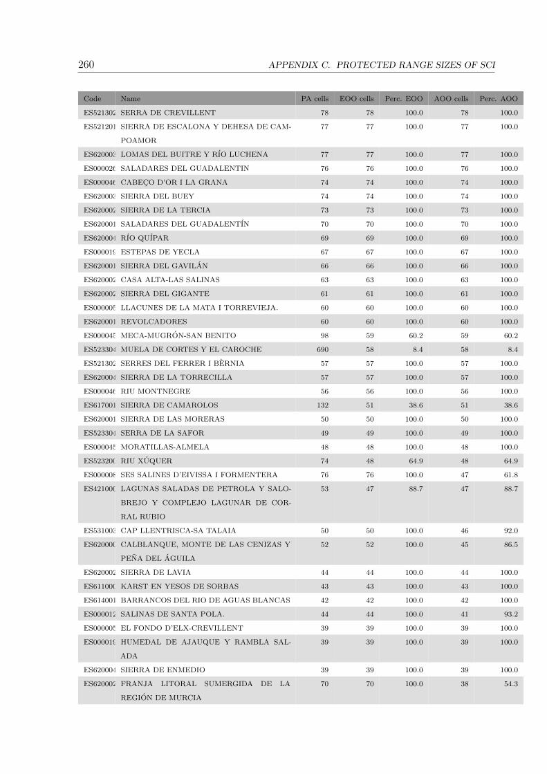
260 APPENDIX C. PROTECTED RANGE SIZES OF SCI
Code Name PA cells EOO cells Perc. EOO AOO cells Perc. AOO
ES5213022SERRA DE CREVILLENT 78 78 100.0 78 100.0
ES5212012SIERRA DE ESCALONA Y DEHESA DE CAM-
POAMOR
77 77 100.0 77 100.0
ES6200034LOMAS DEL BUITRE Y RIO LUCHENA 77 77 100.0 77 100.0
ES0000268SALADARES DEL GUADALENTIN 76 76 100.0 76 100.0
ES0000463CABECO D’OR I LA GRANA 74 74 100.0 74 100.0
ES6200036SIERRA DEL BUEY 74 74 100.0 74 100.0
ES6200023SIERRA DE LA TERCIA 73 73 100.0 73 100.0
ES6200014SALADARES DEL GUADALENTIN 70 70 100.0 70 100.0
ES6200043RIO QUIPAR 69 69 100.0 69 100.0
ES0000196ESTEPAS DE YECLA 67 67 100.0 67 100.0
ES6200019SIERRA DEL GAVILAN 66 66 100.0 66 100.0
ES6200020CASA ALTA-LAS SALINAS 63 63 100.0 63 100.0
ES6200022SIERRA DEL GIGANTE 61 61 100.0 61 100.0
ES0000059LLACUNES DE LA MATA I TORREVIEJA. 60 60 100.0 60 100.0
ES6200016REVOLCADORES 60 60 100.0 60 100.0
ES0000452MECA-MUGRON-SAN BENITO 98 59 60.2 59 60.2
ES5233040MUELA DE CORTES Y EL CAROCHE 690 58 8.4 58 8.4
ES5213020SERRES DEL FERRER I BERNIA 57 57 100.0 57 100.0
ES6200047SIERRA DE LA TORRECILLA 57 57 100.0 57 100.0
ES0000460RIU MONTNEGRE 56 56 100.0 56 100.0
ES6170012SIERRA DE CAMAROLOS 132 51 38.6 51 38.6
ES6200011SIERRA DE LAS MORERAS 50 50 100.0 50 100.0
ES5233041SERRA DE LA SAFOR 49 49 100.0 49 100.0
ES0000456MORATILLAS-ALMELA 48 48 100.0 48 100.0
ES5232007RIU XUQUER 74 48 64.9 48 64.9
ES0000084SES SALINES D’EIVISSA I FORMENTERA 76 76 100.0 47 61.8
ES4210004LAGUNAS SALADAS DE PETROLA Y SALO-
BREJO Y COMPLEJO LAGUNAR DE COR-
RAL RUBIO
53 47 88.7 47 88.7
ES5310032CAP LLENTRISCA-SA TALAIA 50 50 100.0 46 92.0
ES6200001CALBLANQUE, MONTE DE LAS CENIZAS Y
PENA DEL AGUILA
52 52 100.0 45 86.5
ES6200021SIERRA DE LAVIA 44 44 100.0 44 100.0
ES6110002KARST EN YESOS DE SORBAS 43 43 100.0 43 100.0
ES6140015BARRANCOS DEL RIO DE AGUAS BLANCAS 42 42 100.0 42 100.0
ES0000120SALINAS DE SANTA POLA. 44 44 100.0 41 93.2
ES0000058EL FONDO D’ELX-CREVILLENT 39 39 100.0 39 100.0
ES0000195HUMEDAL DE AJAUQUE Y RAMBLA SAL-
ADA
39 39 100.0 39 100.0
ES6200046SIERRA DE ENMEDIO 39 39 100.0 39 100.0
ES6200029FRANJA LITORAL SUMERGIDA DE LA
REGION DE MURCIA
70 70 100.0 38 54.3
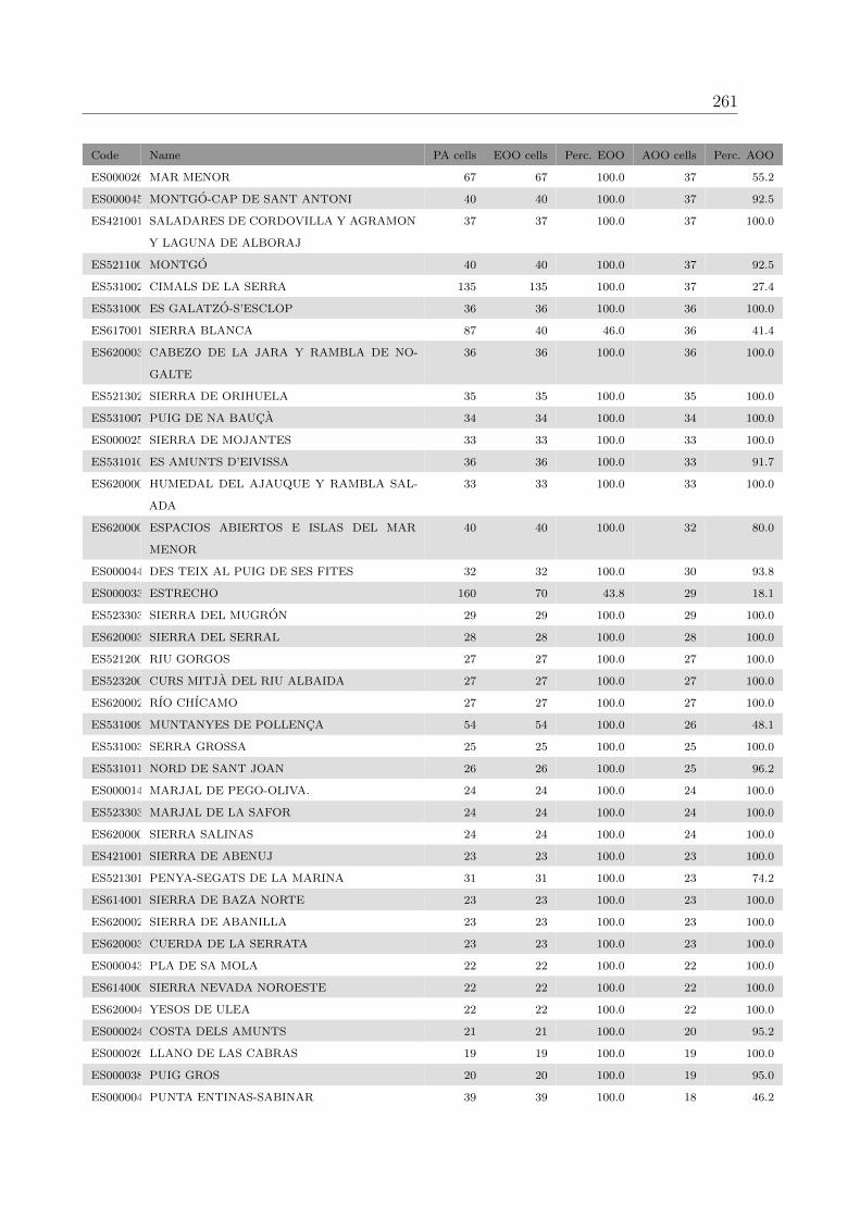
261
Code Name PA cells EOO cells Perc. EOO AOO cells Perc. AOO
ES0000260MAR MENOR 67 67 100.0 37 55.2
ES0000454MONTGO-CAP DE SANT ANTONI 40 40 100.0 37 92.5
ES4210011SALADARES DE CORDOVILLA Y AGRAMON
Y LAGUNA DE ALBORAJ
37 37 100.0 37 100.0
ES5211007MONTGO 40 40 100.0 37 92.5
ES5310027CIMALS DE LA SERRA 135 135 100.0 37 27.4
ES5310008ES GALATZO-S’ESCLOP 36 36 100.0 36 100.0
ES6170011SIERRA BLANCA 87 40 46.0 36 41.4
ES6200039CABEZO DE LA JARA Y RAMBLA DE NO-
GALTE
36 36 100.0 36 100.0
ES5213026SIERRA DE ORIHUELA 35 35 100.0 35 100.0
ES5310079PUIG DE NA BAUCA 34 34 100.0 34 100.0
ES0000259SIERRA DE MOJANTES 33 33 100.0 33 100.0
ES5310105ES AMUNTS D’EIVISSA 36 36 100.0 33 91.7
ES6200005HUMEDAL DEL AJAUQUE Y RAMBLA SAL-
ADA
33 33 100.0 33 100.0
ES6200006ESPACIOS ABIERTOS E ISLAS DEL MAR
MENOR
40 40 100.0 32 80.0
ES0000440DES TEIX AL PUIG DE SES FITES 32 32 100.0 30 93.8
ES0000337ESTRECHO 160 70 43.8 29 18.1
ES5233034SIERRA DEL MUGRON 29 29 100.0 29 100.0
ES6200037SIERRA DEL SERRAL 28 28 100.0 28 100.0
ES5212004RIU GORGOS 27 27 100.0 27 100.0
ES5232008CURS MITJA DEL RIU ALBAIDA 27 27 100.0 27 100.0
ES6200028RIO CHICAMO 27 27 100.0 27 100.0
ES5310092MUNTANYES DE POLLENCA 54 54 100.0 26 48.1
ES5310034SERRA GROSSA 25 25 100.0 25 100.0
ES5310112NORD DE SANT JOAN 26 26 100.0 25 96.2
ES0000147MARJAL DE PEGO-OLIVA. 24 24 100.0 24 100.0
ES5233030MARJAL DE LA SAFOR 24 24 100.0 24 100.0
ES6200008SIERRA SALINAS 24 24 100.0 24 100.0
ES4210010SIERRA DE ABENUJ 23 23 100.0 23 100.0
ES5213018PENYA-SEGATS DE LA MARINA 31 31 100.0 23 74.2
ES6140010SIERRA DE BAZA NORTE 23 23 100.0 23 100.0
ES6200027SIERRA DE ABANILLA 23 23 100.0 23 100.0
ES6200038CUERDA DE LA SERRATA 23 23 100.0 23 100.0
ES0000439PLA DE SA MOLA 22 22 100.0 22 100.0
ES6140009SIERRA NEVADA NOROESTE 22 22 100.0 22 100.0
ES6200042YESOS DE ULEA 22 22 100.0 22 100.0
ES0000241COSTA DELS AMUNTS 21 21 100.0 20 95.2
ES0000263LLANO DE LAS CABRAS 19 19 100.0 19 100.0
ES0000381PUIG GROS 20 20 100.0 19 95.0
ES0000048PUNTA ENTINAS-SABINAR 39 39 100.0 18 46.2
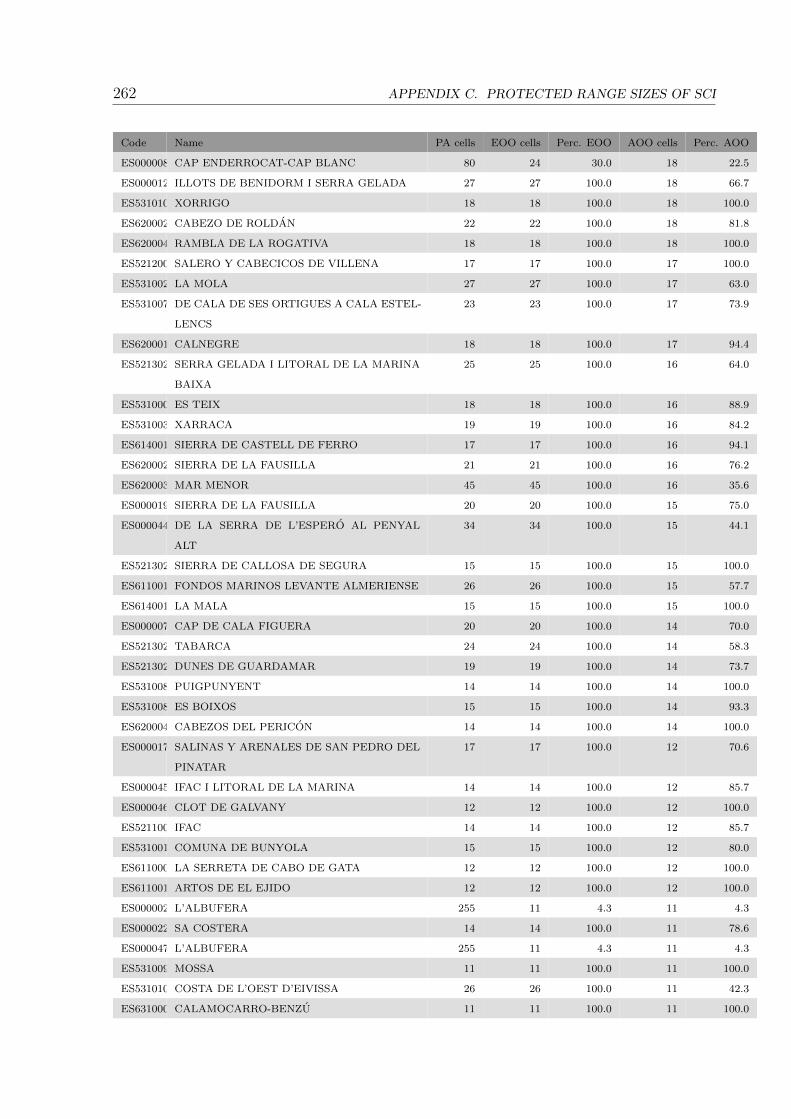
262 APPENDIX C. PROTECTED RANGE SIZES OF SCI
Code Name PA cells EOO cells Perc. EOO AOO cells Perc. AOO
ES0000081CAP ENDERROCAT-CAP BLANC 80 24 30.0 18 22.5
ES0000121ILLOTS DE BENIDORM I SERRA GELADA 27 27 100.0 18 66.7
ES5310102XORRIGO 18 18 100.0 18 100.0
ES6200024CABEZO DE ROLDAN 22 22 100.0 18 81.8
ES6200041RAMBLA DE LA ROGATIVA 18 18 100.0 18 100.0
ES5212007SALERO Y CABECICOS DE VILLENA 17 17 100.0 17 100.0
ES5310024LA MOLA 27 27 100.0 17 63.0
ES5310078DE CALA DE SES ORTIGUES A CALA ESTEL-
LENCS
23 23 100.0 17 73.9
ES6200012CALNEGRE 18 18 100.0 17 94.4
ES5213021SERRA GELADA I LITORAL DE LA MARINA
BAIXA
25 25 100.0 16 64.0
ES5310009ES TEIX 18 18 100.0 16 88.9
ES5310033XARRACA 19 19 100.0 16 84.2
ES6140011SIERRA DE CASTELL DE FERRO 17 17 100.0 16 94.1
ES6200025SIERRA DE LA FAUSILLA 21 21 100.0 16 76.2
ES6200030MAR MENOR 45 45 100.0 16 35.6
ES0000199SIERRA DE LA FAUSILLA 20 20 100.0 15 75.0
ES0000442DE LA SERRA DE L’ESPERO AL PENYAL
ALT
34 34 100.0 15 44.1
ES5213023SIERRA DE CALLOSA DE SEGURA 15 15 100.0 15 100.0
ES6110010FONDOS MARINOS LEVANTE ALMERIENSE 26 26 100.0 15 57.7
ES6140012LA MALA 15 15 100.0 15 100.0
ES0000074CAP DE CALA FIGUERA 20 20 100.0 14 70.0
ES5213024TABARCA 24 24 100.0 14 58.3
ES5213025DUNES DE GUARDAMAR 19 19 100.0 14 73.7
ES5310080PUIGPUNYENT 14 14 100.0 14 100.0
ES5310083ES BOIXOS 15 15 100.0 14 93.3
ES6200040CABEZOS DEL PERICON 14 14 100.0 14 100.0
ES0000175SALINAS Y ARENALES DE SAN PEDRO DEL
PINATAR
17 17 100.0 12 70.6
ES0000459IFAC I LITORAL DE LA MARINA 14 14 100.0 12 85.7
ES0000462CLOT DE GALVANY 12 12 100.0 12 100.0
ES5211009IFAC 14 14 100.0 12 85.7
ES5310010COMUNA DE BUNYOLA 15 15 100.0 12 80.0
ES6110007LA SERRETA DE CABO DE GATA 12 12 100.0 12 100.0
ES6110014ARTOS DE EL EJIDO 12 12 100.0 12 100.0
ES0000023L’ALBUFERA 255 11 4.3 11 4.3
ES0000225SA COSTERA 14 14 100.0 11 78.6
ES0000471L’ALBUFERA 255 11 4.3 11 4.3
ES5310091MOSSA 11 11 100.0 11 100.0
ES5310104COSTA DE L’OEST D’EIVISSA 26 26 100.0 11 42.3
ES6310001CALAMOCARRO-BENZU 11 11 100.0 11 100.0
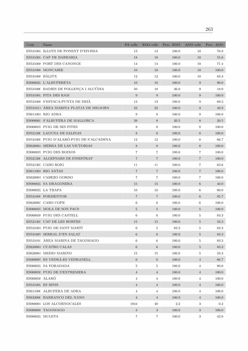
263
Code Name PA cells EOO cells Perc. EOO AOO cells Perc. AOO
ES5310023ILLOTS DE PONENT D’EIVISSA 13 13 100.0 10 76.9
ES5310025CAP DE BARBARIA 18 18 100.0 10 55.6
ES5310081PORT DES CANONGE 14 14 100.0 10 71.4
ES5310085MONCAIRE 10 10 100.0 10 100.0
ES5310087BALITX 12 12 100.0 10 83.3
ES0000226L’ALBUFERETA 10 10 100.0 9 90.0
ES5310005BADIES DE POLLENCA I ALCUDIA 50 18 36.0 9 18.0
ES5310026FITA DES RAM 9 9 100.0 9 100.0
ES5310082S’ESTACA-PUNTA DE DEIA 13 13 100.0 9 69.2
ES5310111AREA MARINA PLATJA DE MIGJORN 22 22 100.0 9 40.9
ES6110018RIO ADRA 9 9 100.0 9 100.0
ES0000038S’ALBUFERA DE MALLORCA 39 8 20.5 8 20.5
ES0000379PUIG DE SES FITES 8 8 100.0 8 100.0
ES5212006LAGUNA DE SALINAS 8 8 100.0 8 100.0
ES5310090PUIG D’ALARO-PUIG DE S’ALCADENA 12 12 100.0 8 66.7
ES6200044SIERRA DE LAS VICTORIAS 8 8 100.0 8 100.0
ES0000378PUIG DES BOIXOS 7 7 100.0 7 100.0
ES5212009ALGEPSARS DE FINESTRAT 7 7 100.0 7 100.0
ES5213033CABO ROIG 11 11 100.0 7 63.6
ES6110017RIO ANTAS 7 7 100.0 7 100.0
ES6200013CABEZO GORDO 7 7 100.0 7 100.0
ES0000221SA DRAGONERA 15 15 100.0 6 40.0
ES0000222LA TRAPA 10 10 100.0 6 60.0
ES5310093FORMENTOR 7 7 100.0 6 85.7
ES6200031CABO COPE 6 6 100.0 6 100.0
ES0000377MOLA DE SON PACS 5 5 100.0 5 100.0
ES0000383PUIG DES CASTELL 6 6 100.0 5 83.3
ES5213032CAP DE LES HORTES 15 15 100.0 5 33.3
ES5310015PUIG DE SANT MARTI 6 5 83.3 5 83.3
ES5310076SERRAL D’EN SALAT 6 6 100.0 5 83.3
ES5310107AREA MARINA DE TAGOMAGO 6 6 100.0 5 83.3
ES6200010CUATRO CALAS 6 6 100.0 5 83.3
ES6200048MEDIO MARINO 15 15 100.0 5 33.3
ES0000078ES VEDRA-ES VEDRANELL 6 6 100.0 4 66.7
ES0000223SA FORADADA 5 5 100.0 4 80.0
ES0000380PUIG DE S’EXTREMERA 4 4 100.0 4 100.0
ES0000382ALARO 4 4 100.0 4 100.0
ES5310028ES BINIS 4 4 100.0 4 100.0
ES6110001ALBUFERA DE ADRA 4 4 100.0 4 100.0
ES6320002BARRANCO DEL NANO 4 4 100.0 4 100.0
ES0000049LOS ALCORNOCALES 1844 40 2.2 3 0.2
ES0000082TAGOMAGO 3 3 100.0 3 100.0
ES0000224MULETA 7 7 100.0 3 42.9

264 APPENDIX C. PROTECTED RANGE SIZES OF SCI
Code Name PA cells EOO cells Perc. EOO AOO cells Perc. AOO
ES5310031PORROIG 3 3 100.0 3 100.0
ES5310089BINIARROI 11 11 100.0 3 27.3
ES5310109AREA MARINA DE CALA SAONA 4 4 100.0 3 75.0
ES6170002ACANTILADOS DE MARO-CERRO GORDO 15 15 100.0 3 20.0
ES0000214ILLOTS DE TABARCA 12 12 100.0 2 16.7
ES5310084TORRE PICADA 5 5 100.0 2 40.0
ES5310086MONNABER 2 2 100.0 2 100.0
ES5310088GORG BLAU 6 6 100.0 2 33.3
ES5310106AREA MARINA DE SES MARGALIDES 2 2 100.0 2 100.0
ES5310108AREA MARINA DEL CAP MARTINET 7 7 100.0 2 28.6
ES6140014ACANTILADOS Y FONDOS MARINOS DE
CALAHONDA-CASTELL DE FERRO
7 7 100.0 2 28.6
ES6160015RIO GUADIANA MENOR - TRAMO SUPE-
RIOR
2 2 100.0 2 100.0
ES6170028RIO GUADALMEDINA 4 4 100.0 2 50.0
ES6170037EL SALADILLO - PUNTA DE BANOS 5 5 100.0 2 40.0
ES6200007ISLAS E ISLOTES DEL LITORAL
MEDITERRANEO
4 4 100.0 2 50.0
ES6310002ZONA MARITIMO-TERRESTRE DEL MONTE
HACHO
6 6 100.0 2 33.3
ES6320001ZONA MARITIMO TERRESTRE DE LOS
ACANTILADOS DE AGUADU
2 2 100.0 2 100.0
ES0000197ACANTILADOS DEL MONTE HACHO 4 4 100.0 1 25.0
ES5212010ARENAL DE PETRER 1 1 100.0 1 100.0
ES5214002TUNEL DE CANALS 1 1 100.0 1 100.0
ES5214004COVA JOLIANA 1 1 100.0 1 100.0
ES5232009SERRA DEL CASTELL DE XATIVA 1 1 100.0 1 100.0
ES5233049COVA DE LES RATES PENADES (ROTOVA) 1 1 100.0 1 100.0
ES5310037BASSES DE LA MARINA DE LLUCMAJOR 3 1 33.3 1 33.3
ES5310040COVA DE LES MARAVELLES 1 1 100.0 1 100.0
ES5310042AVENC D’EN CORBERA 1 1 100.0 1 100.0
ES5310057COVA DE CAL PESSO 1 1 100.0 1 100.0
ES5310059COVA DE LLENAIRE 1 1 100.0 1 100.0
ES5310062ES BUFADOR DE SON BERENGUER 1 1 100.0 1 100.0
ES5310063COVA DE CAN MILLO O DE COA NEGRINA 1 1 100.0 1 100.0
ES5310064AVENC DE SON POU 1 1 100.0 1 100.0
ES5310123BASSA DE FORMENTERA 1 1 100.0 1 100.0
ES6110016RAMBLA DE AREJOS 1 1 100.0 1 100.0
ES6120003ESTUARIO DEL RIO GUADIARO 3 2 66.7 1 33.3
ES6170021RIO GUADALMINA 1 1 100.0 1 100.0
ES6170022RIO FUENGIROLA 7 7 100.0 1 14.3
ES6170030CALAHONDA 7 7 100.0 1 14.3
ES6200032MINAS DE LA CELIA 1 1 100.0 1 100.0

265
Code Name PA cells EOO cells Perc. EOO AOO cells Perc. AOO
ES0000036ISLAS CHAFARINAS 3 3 100.0 0 0.0
ES0000200ISLA GROSA 1 1 100.0 0 0.0
ES0000242ILLOTS DE SANTA EULARIA, RODONA I ES
CANA
2 2 100.0 0 0.0
ES0000256ISLAS HORMIGAS 1 1 100.0 0 0.0
ES5310058COVA DE CAN SION 1 1 100.0 0 0.0
ES5310060COVA MORELLA 1 1 100.0 0 0.0
ES5310103AREA MARINA CAP DE CALA FIGUERA 1 1 100.0 0 0.0
ES5310110AREA MARINA PLATJA DE TRAMUNTANA 1 1 100.0 0 0.0
ES6110009FONDOS MARINOS DE PUNTA ENTINAS-
SABINAR
16 16 100.0 0 0.0
ES6120006MARISMAS DEL RIO PALMONES 4 1 25.0 0 0.0
ES6140013FONDOS MARINOS TESORILLO-
SALOBRENA
6 6 100.0 0 0.0
ES6140016ACANTILADOS Y FONDOS MARINOS DE LA
PUNTA DE LA MONA
2 2 100.0 0 0.0
ES6160011RIO GUADIANA MENOR - TRAMO INFE-
RIOR
5 4 80.0 0 0.0
ES6170033RIOS GUADALHORCE, FABALAS Y
PEREILAS
12 5 41.7 0 0.0
ES6300001ISLAS CHAFARINAS 3 3 100.0 0 0.0
SPAIN TOTAL: 31629 23926 75.6 22912 72.4
OVERALL NATURA 2000 TOTAL: 31629 23926 75.6 22912 72.4

266 APPENDIX C. PROTECTED RANGE SIZES OF SCI
Table C.12: Euphorbia squamigera PSA protection by North African protected areas
Code Type Name PA cells PSA cells Perc. PSA
ALGERIA
902847 Wetlands of International
Importance (Ramsar)
Garaet Guellif 268 259 96.6
101170 National Park Tlemcen 182 182 100.0
14903 Breeding Station Tlemcen 182 182 100.0
13697 Hunting Reserve Tlemcen 182 182 100.0
902845 Wetlands of International
Importance (Ramsar)
Garaet Annk Djemel et El Merhsel 206 165 80.1
900713 UNESCO-MAB Biosphere
Reserve
Chrea 568 138 24.3
9740 National Park Chrea 568 138 24.3
26620 UNESCO-MAB Biosphere
Reserve
El Kala 897 134 14.9
9741 National Park El Kala 897 134 14.9
14909 Marine Park El Kala 897 134 14.9
9742 National Park Belezma 218 103 47.2
902846 Wetlands of International
Importance (Ramsar)
Garaet El Taref 369 87 23.6
901223 Wetlands of International
Importance (Ramsar)
Chott de Zehrez Chergui 552 85 15.4
9758 Nature Reserve Macta 207 78 37.7
4118 National Park Djurdjura 562 74 13.2
145569 UNESCO-MAB Biosphere
Reserve
Djurdjura 562 74 13.2
902852 Wetlands of International
Importance (Ramsar)
Sebkhet Bazer 58 58 100.0
900575 Wetlands of International
Importance (Ramsar)
Marais de la Macta 489 55 11.2
9743 National Park Taza 52 51 98.1
902530 UNESCO-MAB Biosphere
Reserve
Taza 52 51 98.1
12350 Strict Nature Reserve Babor 49 49 100.0
902844 Wetlands of International
Importance (Ramsar)
Dayet El Ferd 46 46 100.0
900574 Wetlands of International
Importance (Ramsar)
Complexe de zones humides de la plaine de
Guerbes-Sanhadja
432 39 9.0
14904 Breeding Station Boumerdes 100 37 37.0
902853 Wetlands of International
Importance (Ramsar)
Sebkhet El Hamiet 37 37 100.0
72354 National Park Djebel Aissa 44 36 81.8

267
Code Type Name PA cells PSA cells Perc. PSA
3369 Park Tipasa-Chenoua Terrestrial and Marine 62 27 43.5
902843 Wetlands of International
Importance (Ramsar)
Chott Tinsilt 31 20 64.5
9748 Regional Park Seraidi P 40 20 50.0
72363 National Park Tipaza Chenoua 49 19 38.8
72355 National Park Edough 36 16 44.4
902531 UNESCO-MAB Biosphere
Reserve
Gouraya 18 12 66.7
9747 National Park Gouraya 18 12 66.7
901231 Wetlands of International
Importance (Ramsar)
Marais de la Mekhada 106 10 9.4
9755 Marine Park Jijel 9 9 100.0
72356 National Park Naama 9 9 100.0
900576 Wetlands of International
Importance (Ramsar)
Sebkha d’Oran 617 9 1.5
14905 Other Area Setif 9 9 100.0
4120 Nature Reserve Beni-Salah 34 6 17.6
14906 Other Area Mostaganem 6 6 100.0
72362 National Park Tigzirt 3 3 100.0
12354 Breeding Station Reghaia 4 2 50.0
901224 Wetlands of International
Importance (Ramsar)
Chott de Zehrez Gharbi 568 1 0.2
12355 Other Area Lac Tonga 34 1 2.9
72361 National Park La Salamandre 4 1 25.0
ALGERIA TOTAL: 10333 2800 27.1
MOROCCO
168216 UNESCO-MAB Biosphere
Reserve
Arganeraie 20690 16457 79.5
220265 UNESCO-MAB Biosphere
Reserve
Oasis de Sud Morocain 62356 7899 12.7
4114 National Park Toubkal 1058 994 94.0
313472 Natural Park Talassemtane 729 564 77.4
31073 National Park Parc de Haut Atlas Oriental 438 437 99.8
11697 National Park Souss-Massa 463 380 82.1
4115 National Park Tazekka 459 367 80.0
17742 National Park Talassantane 648 293 45.2
11690 Botanical Reserve Talassantane 648 293 45.2
29969 National Park Al Hoceima 271 269 99.3
20371 Marine Reserve Bokkoyas 268 266 99.3
11698 Biological Reserve Bokkoyas 268 266 99.3
15089 National Park Ifrane 621 234 37.7
313471 Natural Park Ifrane 621 234 37.7

268 APPENDIX C. PROTECTED RANGE SIZES OF SCI
Code Type Name PA cells PSA cells Perc. PSA
902705 Wetlands of International
Importance (Ramsar)
Complexe de Sidi Moussa-Walidia 89 85 95.5
11689 Biological Reserve Merja Zerga 71 63 88.7
17710 Wetlands of International
Importance (Ramsar)
Merja Zerga 71 63 88.7
902707 Wetlands of International
Importance (Ramsar)
Complexe du bas Tahaddart 72 51 70.8
11691 Permanent Hunting Re-
serve
Sidi Boughaba 51 43 84.3
32551 Biological Reserve Sidi Boughaba 51 43 84.3
902709 Wetlands of International
Importance (Ramsar)
Embouchure de la Moulouya 41 40 97.6
902703 Wetlands of International
Importance (Ramsar)
Barrage Mohammed V 64 39 60.9
902715 Wetlands of International
Importance (Ramsar)
Sebkha Bou Areg 55 31 56.4
11688 Hunting Reserve Mouley Bousalham 34 27 79.4
15102 Nature Reserve Merja Daoura (Merja Sidi Mohammed Ben
Mansour) NR
82 26 31.7
15103 Reserve Rio Martine lagoon 40 23 57.5
11684 Permanent Hunting Re-
serve
Takherkhort 20 20 100.0
902717 Wetlands of International
Importance (Ramsar)
Zones humides de l’oued El Maleh 20 20 100.0
902718 Wetlands of International
Importance (Ramsar)
Zones humides de Souss-Massa 18 18 100.0
902704 Wetlands of International
Importance (Ramsar)
Cap des Trois Fourches 26 17 65.4
17711 Wetlands of International
Importance (Ramsar)
Merja Sidi Boughaba 17 15 88.2
902711 Wetlands of International
Importance (Ramsar)
Lacs Isly-Tislite 14 14 100.0
12381 Biological Reserve Oued Massa 11 11 100.0
902699 Wetlands of International
Importance (Ramsar)
Aguelmams Sidi Ali - Tifounassine 9 9 100.0
13423 Reserve Oualidia et Sidi Moussa 9 9 100.0
15111 Hunting Reserve Aguelman Sidi Ali 8 8 100.0
902700 Wetlands of International
Importance (Ramsar)
Archipel et dunes d’Essawira 13 8 61.5
15113 Hunting Reserve Dayet Ifrah 8 8 100.0
15095 Nature Reserve Lac Iseli 8 8 100.0
15117 Nature Reserve El Merja (Sidi Moussa region) 7 7 100.0
15112 Hunting Reserve Dayet el Hachlef 6 6 100.0

269
Code Type Name PA cells PSA cells Perc. PSA
13699 Reserve Tidhirine 6 6 100.0
15093 Hunting Reserve Dayet Agoulman 4 4 100.0
15116 Nature Reserve El Holba 4 4 100.0
17712 Wetlands of International
Importance (Ramsar)
Lac d’Afennourir 19 4 21.1
15096 Nature Reserve Lac Tislit 4 4 100.0
15106 Nature Reserve Oued Loukkos 5 4 80.0
15109 Hunting Reserve Dayet Afougha 3 3 100.0
15099 Nature Reserve Nador 21 3 14.3
902706 Wetlands of International
Importance (Ramsar)
Complexe du bas Loukkos 49 2 4.1
15108 Hunting Reserve Dayet Aaoua 2 2 100.0
902997 UNESCO-MAB Biosphere
Reserve
Intercontinental BR of the Mediterranean 8 2 25.0
15115 Nature Reserve Sidi Rahat 5 2 40.0
15118 Nature Reserve Aguelmam Tifounassine 1 1 100.0
11692 Permanent Hunting Re-
serve
Ile de Skhirate 1 1 100.0
MOROCCO TOTAL: 90585 29707 32.8
TUNISIA
903084 Wetlands of International
Importance (Ramsar)
Sebkhet Kelbia 238 232 97.5
15185 Wetland Zone of National
Importance
Sebkhet Kelbia 238 232 97.5
15188 Nature Reserve Lac Bizerte 90 71 78.9
15182 Nature Reserve Medjerda Estuary 66 61 92.4
15187 Wetland Zone of National
Importance
Sebkhet-Sidi-El-Hani 388 59 15.2
903080 Wetlands of International
Importance (Ramsar)
Lagune de Ghar el Melh et DElta de la
Mejerda
71 58 81.7
32554 Wetland Zone of National
Importance
Sebkhet Ariana 43 43 100.0
903086 Wetlands of International
Importance (Ramsar)
Sebkhet Sejoumi 42 42 100.0
15183 Wetland Zone of National
Importance
Sebkhet es Sedjoumi 36 36 100.0
12390 National Park Boukornine 24 24 100.0
15194 Wetland Zone of National
Importance
Sebkha Halk el Menzel 20 20 100.0
15184 Wetland Zone of National
Importance
Sebkhet Kourzia 25 19 76.0

270 APPENDIX C. PROTECTED RANGE SIZES OF SCI
Code Type Name PA cells PSA cells Perc. PSA
903072 Wetlands of International
Importance (Ramsar)
Barrage Lebna 16 16 100.0
903087 Wetlands of International
Importance (Ramsar)
Sebkhet Soliman 14 14 100.0
17744 National Park El-Feidja 39 10 25.6
903081 Wetlands of International
Importance (Ramsar)
Lagunes du Cap Bon oriental 8 8 100.0
15193 Nature Reserve Cap Bon peninsula 6 6 100.0
15202 Nature Reserve Djebel Zaghouan 6 6 100.0
12392 Faunal Reserve Dar Chichou 4 4 100.0
2115 UNESCO-MAB Biosphere
Reserve
Iles Zembra et Zembretta 8 2 25.0
365017 Barcelona Convention Zembra and Zembretta 8 2 25.0
942 National Park Zembra and Zembretta 8 2 25.0
15203 Nature Reserve Dar Fatma 1 1 100.0
101847 Natural Reserve Grotte de Chauve souris d’El Haouaria 1 1 100.0
941 National Park Ichkeul 150 1 0.7
17719 Wetlands of International
Importance (Ramsar)
Ichkeul 150 1 0.7
TUNISIA TOTAL: 1700 971 57.1
OVERALL NORTH AFRICAN TOTAL: 102618 33478 32.6
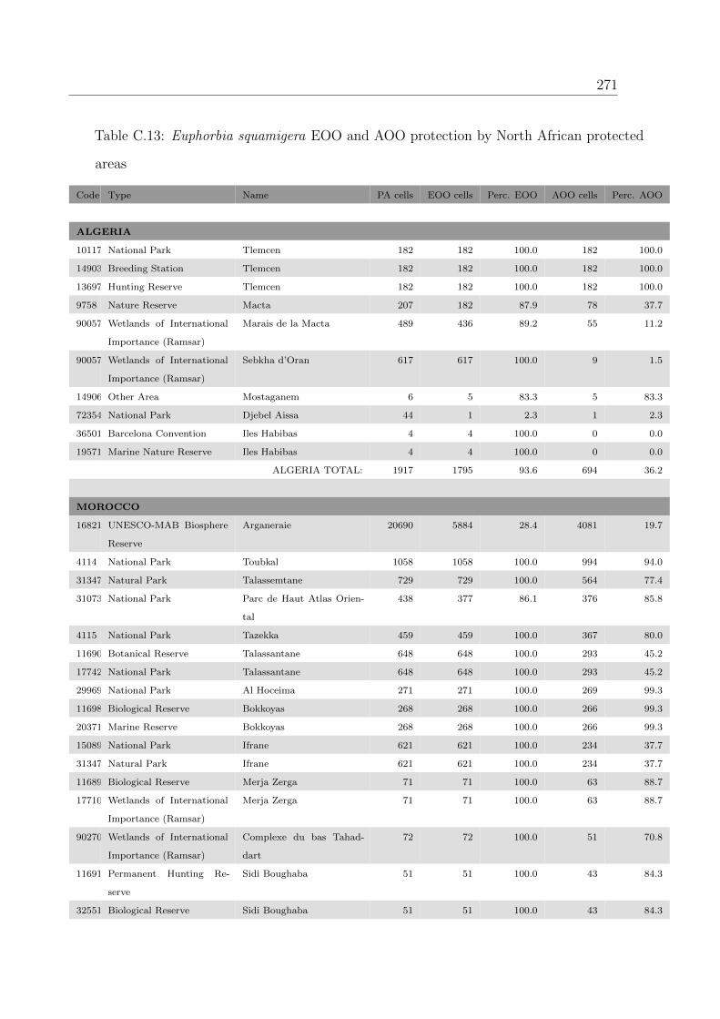
271
Table C.13: Euphorbia squamigera EOO and AOO protection by North African protected
areas
Code Type Name PA cells EOO cells Perc. EOO AOO cells Perc. AOO
ALGERIA
101170National Park Tlemcen 182 182 100.0 182 100.0
14903 Breeding Station Tlemcen 182 182 100.0 182 100.0
13697 Hunting Reserve Tlemcen 182 182 100.0 182 100.0
9758 Nature Reserve Macta 207 182 87.9 78 37.7
900575Wetlands of International
Importance (Ramsar)
Marais de la Macta 489 436 89.2 55 11.2
900576Wetlands of International
Importance (Ramsar)
Sebkha d’Oran 617 617 100.0 9 1.5
14906 Other Area Mostaganem 6 5 83.3 5 83.3
72354 National Park Djebel Aissa 44 1 2.3 1 2.3
365019Barcelona Convention Iles Habibas 4 4 100.0 0 0.0
19571 Marine Nature Reserve Iles Habibas 4 4 100.0 0 0.0
ALGERIA TOTAL: 1917 1795 93.6 694 36.2
MOROCCO
168216UNESCO-MAB Biosphere
Reserve
Arganeraie 20690 5884 28.4 4081 19.7
4114 National Park Toubkal 1058 1058 100.0 994 94.0
313472Natural Park Talassemtane 729 729 100.0 564 77.4
31073 National Park Parc de Haut Atlas Orien-
tal
438 377 86.1 376 85.8
4115 National Park Tazekka 459 459 100.0 367 80.0
11690 Botanical Reserve Talassantane 648 648 100.0 293 45.2
17742 National Park Talassantane 648 648 100.0 293 45.2
29969 National Park Al Hoceima 271 271 100.0 269 99.3
11698 Biological Reserve Bokkoyas 268 268 100.0 266 99.3
20371 Marine Reserve Bokkoyas 268 268 100.0 266 99.3
15089 National Park Ifrane 621 621 100.0 234 37.7
313471Natural Park Ifrane 621 621 100.0 234 37.7
11689 Biological Reserve Merja Zerga 71 71 100.0 63 88.7
17710 Wetlands of International
Importance (Ramsar)
Merja Zerga 71 71 100.0 63 88.7
902707Wetlands of International
Importance (Ramsar)
Complexe du bas Tahad-
dart
72 72 100.0 51 70.8
11691 Permanent Hunting Re-
serve
Sidi Boughaba 51 51 100.0 43 84.3
32551 Biological Reserve Sidi Boughaba 51 51 100.0 43 84.3

272 APPENDIX C. PROTECTED RANGE SIZES OF SCI
Code Type Name PA cells EOO cells Perc. EOO AOO cells Perc. AOO
902709Wetlands of International
Importance (Ramsar)
Embouchure de la
Moulouya
41 41 100.0 40 97.6
902703Wetlands of International
Importance (Ramsar)
Barrage Mohammed V 64 64 100.0 39 60.9
902715Wetlands of International
Importance (Ramsar)
Sebkha Bou Areg 55 55 100.0 31 56.4
11688 Hunting Reserve Mouley Bousalham 34 34 100.0 27 79.4
15102 Nature Reserve Merja Daoura (Merja Sidi
Mohammed Ben Mansour)
NR
82 82 100.0 26 31.7
15103 Reserve Rio Martine lagoon 40 40 100.0 23 57.5
11684 Permanent Hunting Re-
serve
Takherkhort 20 20 100.0 20 100.0
902704Wetlands of International
Importance (Ramsar)
Cap des Trois Fourches 26 26 100.0 17 65.4
17711 Wetlands of International
Importance (Ramsar)
Merja Sidi Boughaba 17 17 100.0 15 88.2
902711Wetlands of International
Importance (Ramsar)
Lacs Isly-Tislite 14 14 100.0 14 100.0
902699Wetlands of International
Importance (Ramsar)
Aguelmams Sidi Ali -
Tifounassine
9 9 100.0 9 100.0
15111 Hunting Reserve Aguelman Sidi Ali 8 8 100.0 8 100.0
15113 Hunting Reserve Dayet Ifrah 8 8 100.0 8 100.0
15095 Nature Reserve Lac Iseli 8 8 100.0 8 100.0
15112 Hunting Reserve Dayet el Hachlef 6 6 100.0 6 100.0
13699 Reserve Tidhirine 6 6 100.0 6 100.0
15093 Hunting Reserve Dayet Agoulman 4 4 100.0 4 100.0
17712 Wetlands of International
Importance (Ramsar)
Lac d’Afennourir 19 19 100.0 4 21.1
15096 Nature Reserve Lac Tislit 4 4 100.0 4 100.0
15106 Nature Reserve Oued Loukkos 5 5 100.0 4 80.0
15109 Hunting Reserve Dayet Afougha 3 3 100.0 3 100.0
15099 Nature Reserve Nador 21 21 100.0 3 14.3
902706Wetlands of International
Importance (Ramsar)
Complexe du bas Loukkos 49 49 100.0 2 4.1
15108 Hunting Reserve Dayet Aaoua 2 2 100.0 2 100.0
902997UNESCO-MAB Biosphere
Reserve
Intercontinental BR of the
Mediterranean
8 8 100.0 2 25.0
15118 Nature Reserve Aguelmam Tifounassine 1 1 100.0 1 100.0
11692 Permanent Hunting Re-
serve
Ile de Skhirate 1 1 100.0 1 100.0
902717Wetlands of International
Importance (Ramsar)
Zones humides de l’oued El
Maleh
20 1 5.0 1 5.0
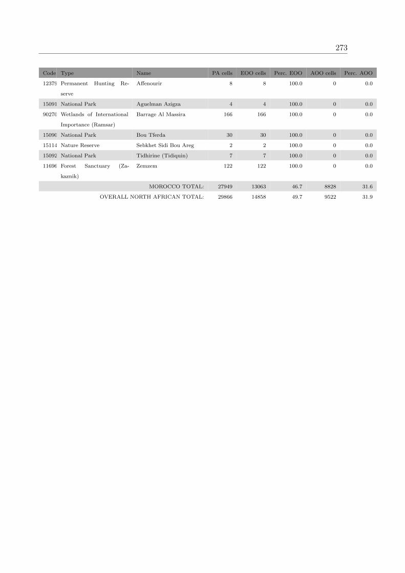
273
Code Type Name PA cells EOO cells Perc. EOO AOO cells Perc. AOO
12379 Permanent Hunting Re-
serve
Affenourir 8 8 100.0 0 0.0
15091 National Park Aguelman Azigza 4 4 100.0 0 0.0
902702Wetlands of International
Importance (Ramsar)
Barrage Al Massira 166 166 100.0 0 0.0
15090 National Park Bou Tferda 30 30 100.0 0 0.0
15114 Nature Reserve Sebkhet Sidi Bou Areg 2 2 100.0 0 0.0
15092 National Park Tidhirine (Tidiquin) 7 7 100.0 0 0.0
11696 Forest Sanctuary (Za-
kaznik)
Zemzem 122 122 100.0 0 0.0
MOROCCO TOTAL: 27949 13063 46.7 8828 31.6
OVERALL NORTH AFRICAN TOTAL: 29866 14858 49.7 9522 31.9

274 APPENDIX C. PROTECTED RANGE SIZES OF SCI
Helianthemum caput-felis
Table C.14: Helianthemum caput-felis PSA protection by Natura 2000
Code Name PA cells PSA cells Perc. PSA
SPAIN
ES0000023 L’ALBUFERA 255 84 32.9
ES0000471 L’ALBUFERA 255 84 32.9
ES0000046 CABO DE GATA-NIJAR 477 70 14.7
ES0000073 COSTA BRAVA DE MALLORCA 143 58 40.6
ES0000081 CAP ENDERROCAT-CAP BLANC 80 58 72.5
ES0000020 DELTA DE L’EBRE 223 57 25.6
ES0000264 SIERRA DE LA MUELA Y CABO TINOSO 147 52 35.4
ES0000084 SES SALINES D’EIVISSA I FORMENTERA 76 47 61.8
ES0000083 ARXIPELAG DE CABRERA 75 42 56.0
ES6200015 LA MUELA Y CABO TINOSO 110 38 34.5
ES6200029 FRANJA LITORAL SUMERGIDA DE LA REGION DE MUR-
CIA
70 38 54.3
ES0000228 CAP DE SES SALINES 60 37 61.7
ES0000260 MAR MENOR 67 37 55.2
ES0000231 DELS ALOCS A FORNELLS 52 35 67.3
ES6200001 CALBLANQUE, MONTE DE LAS CENIZAS Y PENA DEL
AGUILA
52 35 67.3
ES5310105 ES AMUNTS D’EIVISSA 36 33 91.7
ES5310032 CAP LLENTRISCA-SA TALAIA 50 32 64.0
ES6110012 SIERRAS ALMAGRERA, DE LOS PINOS Y EL AGUILON 87 30 34.5
ES0000227 MUNTANYES D’ARTA 129 28 21.7
ES0000024 DONANA 1310 26 2.0
ES0000451 MONTDUVER-MARJAL DE LA SAFOR 149 26 17.4
ES6200006 ESPACIOS ABIERTOS E ISLAS DEL MAR MENOR 40 26 65.0
ES0000318 CABO BUSTO-LUANCO 138 25 18.1
ES5233030 MARJAL DE LA SAFOR 24 23 95.8
ES5310035 AREA MARINA DEL NORD DE MENORCA 34 23 67.6
ES0000317 PENARRONDA-BARAYO 64 22 34.4
ES5310112 NORD DE SANT JOAN 26 22 84.6
ES6110005 SIERRA DE CABRERA-BEDAR 413 22 5.3
ES0000241 COSTA DELS AMUNTS 21 20 95.2
ES0000450 MARJAL I ESTANYS D’ALMENARA 32 19 59.4
ES5223007 MARJAL D’ALMENARA 32 19 59.4
ES5310005 BADIES DE POLLENCA I ALCUDIA 50 19 38.0
ES0000120 SALINAS DE SANTA POLA. 44 18 40.9
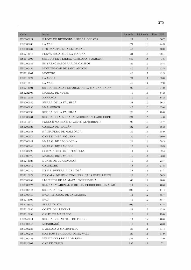
275
Code Name PA cells PSA cells Perc. PSA
ES0000121 ILLOTS DE BENIDORM I SERRA GELADA 27 18 66.7
ES0000230 LA VALL 74 18 24.3
ES0000237 DES CANUTELLS A LLUCALARI 45 18 40.0
ES5213018 PENYA-SEGATS DE LA MARINA 31 18 58.1
ES6170007 SIERRAS DE TEJEDA, ALMIJARA Y ALHAMA 480 18 3.8
ES0000037 ES TRENC-SALOBRAR DE CAMPOS 26 17 65.4
ES0000454 MONTGO-CAP DE SANT ANTONI 40 17 42.5
ES5211007 MONTGO 40 17 42.5
ES5310024 LA MOLA 27 17 63.0
ES5310113 LA VALL 46 17 37.0
ES5213021 SERRA GELADA I LITORAL DE LA MARINA BAIXA 25 16 64.0
ES5222005 MARJAL DE NULES 19 16 84.2
ES5310033 XARRACA 19 16 84.2
ES6200025 SIERRA DE LA FAUSILLA 21 16 76.2
ES6200030 MAR MENOR 45 16 35.6
ES0000199 SIERRA DE LA FAUSILLA 20 15 75.0
ES0000261 SIERRA DE ALMENARA, MORERAS Y CABO COPE 327 15 4.6
ES6110010 FONDOS MARINOS LEVANTE ALMERIENSE 26 15 57.7
ES6200024 CABEZO DE ROLDAN 22 15 68.2
ES0000038 S’ALBUFERA DE MALLORCA 39 14 35.9
ES0000074 CAP DE CALA FIGUERA 20 14 70.0
ES0000147 MARJAL DE PEGO-OLIVA. 24 14 58.3
ES0000148 MARJAL DELS MOROS. 15 14 93.3
ES0000229 COSTA NORD DE CIUTADELLA 17 14 82.4
ES0000470 MARJAL DELS MOROS 15 14 93.3
ES5213025 DUNES DE GUARDAMAR 19 14 73.7
ES6200012 CALNEGRE 18 14 77.8
ES0000235 DE S’ALBUFERA A LA MOLA 41 13 31.7
ES5310078 DE CALA DE SES ORTIGUES A CALA ESTELLENCS 23 13 56.5
ES0000059 LLACUNES DE LA MATA I TORREVIEJA. 60 12 20.0
ES0000175 SALINAS Y ARENALES DE SAN PEDRO DEL PINATAR 17 12 70.6
ES0000444 SERRA D’IRTA 105 12 11.4
ES0000459 IFAC I LITORAL DE LA MARINA 14 12 85.7
ES5211009 IFAC 14 12 85.7
ES5223036 SERRA D’IRTA 105 12 11.4
ES5310030 COSTA DE LLEVANT 28 12 42.9
ES5310098 CALES DE MANACOR 16 12 75.0
ES6140011 SIERRA DE CASTELL DE FERRO 17 12 70.6
ES0000145 MONDRAGO 15 11 73.3
ES0000233 D’ADDAIA A S’ALBUFERA 35 11 31.4
ES0000238 SON BOU I BARRANC DE SA VALL 29 11 37.9
ES0000453 MUNTANYES DE LA MARINA 557 11 2.0
ES5120007 CAP DE CREUS 155 11 7.1

276 APPENDIX C. PROTECTED RANGE SIZES OF SCI
Code Name PA cells PSA cells Perc. PSA
ES5310104 COSTA DE L’OEST D’EIVISSA 26 11 42.3
ES6200011 SIERRA DE LAS MORERAS 50 11 22.0
ES0000060 PRAT DE CABANES I TORREBLANCA. 18 10 55.6
ES0000467 PRAT DE CABANES I TORREBLANCA 18 10 55.6
ES1110005 COSTA DA MORTE 227 10 4.4
ES5120016 EL MONTGRI- LES MEDES - EL BAIX TER 77 10 13.0
ES5212012 SIERRA DE ESCALONA Y DEHESA DE CAMPOAMOR 77 10 13.0
ES5310023 ILLOTS DE PONENT D’EIVISSA 13 10 76.9
ES5310025 CAP DE BARBARIA 18 10 55.6
ES0000239 DE BINIGAUS A CALA MITJANA 48 9 18.8
ES5310068 CAP NEGRE 9 9 100.0
ES5310081 PORT DES CANONGE 14 9 64.3
ES5310111 AREA MARINA PLATJA DE MIGJORN 22 9 40.9
ES6150005 MARISMAS DE ISLA CRISTINA 43 9 20.9
ES0000025 MARISMAS DEL ODIEL 92 8 8.7
ES0000079 LA VICTORIA 16 8 50.0
ES0000232 LA MOLA I S’ALBUFERA DE FORNELLS 29 8 27.6
ES0000372 COSTA DA MARINA OCCIDENTAL 36 8 22.2
ES0000464 SIERRA ESCALONA Y DEHESA DE CAMPOAMOR 136 8 5.9
ES1120017 COSTA DA MARINA OCCIDENTAL 38 8 21.1
ES5213020 SERRES DEL FERRER I BERNIA 57 8 14.0
ES5213024 TABARCA 24 8 33.3
ES5310029 NA BORGES 69 8 11.6
ES5310082 S’ESTACA-PUNTA DE DEIA 13 8 61.5
ES6110008 SIERRAS DE GADOR Y ENIX 598 8 1.3
ES0000226 L’ALBUFERETA 10 7 70.0
ES0000240 COSTA SUD DE CIUTADELLA 25 7 28.0
ES0000443 SUD DE CIUTADELLA 38 7 18.4
ES1110002 COSTA ARTABRA 187 7 3.7
ES5213033 CABO ROIG 11 7 63.6
ES5310074 DE CALA LLUCALARI A CALES COVES 12 7 58.3
ES6150006 MARISMAS DEL RIO PIEDRAS Y FLECHA DEL ROMPIDO 55 7 12.7
ES0000019 AIGUAMOLLS DE L’ALT EMPORDA 89 6 6.7
ES0000221 SA DRAGONERA 15 6 40.0
ES0000222 LA TRAPA 10 6 60.0
ES0000462 CLOT DE GALVANY 12 6 50.0
ES1120005 AS CATEDRAIS 17 6 35.3
ES5140001 LITORAL MERIDIONAL TARRAGONI 20 6 30.0
ES5310008 ES GALATZO-S’ESCLOP 36 6 16.7
ES6200031 CABO COPE 6 6 100.0
ES0000225 SA COSTERA 14 5 35.7
ES0000234 S’ALBUFERA DES GRAU 31 5 16.1
ES5140007 COSTES DEL TARRAGONES 14 5 35.7

277
Code Name PA cells PSA cells Perc. PSA
ES5213032 CAP DE LES HORTES 15 5 33.3
ES5222002 MARJAL DE PENISCOLA 5 5 100.0
ES5310087 BALITX 12 5 41.7
ES5310093 FORMENTOR 7 5 71.4
ES5310107 AREA MARINA DE TAGOMAGO 6 5 83.3
ES6110017 RIO ANTAS 7 5 71.4
ES6200010 CUATRO CALAS 6 5 83.3
ES6200048 MEDIO MARINO 15 5 33.3
ES0000078 ES VEDRA-ES VEDRANELL 6 4 66.7
ES0000176 COSTA DA MORTE (NORTE) 107 4 3.7
ES0000223 SA FORADADA 5 4 80.0
ES1110010 ESTACA DE BARES 25 4 16.0
ES5120013 MASSIS DE LES CADIRETES 122 4 3.3
ES5120015 LITORAL DEL BAIX EMPORDA 51 4 7.8
ES5232007 RIU XUQUER 74 4 5.4
ES5310036 AREA MARINA DEL SUD DE CIUTADELLA 20 4 20.0
ES5310070 PUNTA REDONA-ARENAL D’EN CASTELL 10 4 40.0
ES5310076 SERRAL D’EN SALAT 6 4 66.7
ES5310096 PUNTA DE N’AMER 6 4 66.7
ES6320002 BARRANCO DEL NANO 4 4 100.0
ES0000080 CAP VERMELL 6 3 50.0
ES0000082 TAGOMAGO 3 3 100.0
ES0000085 RIBADEO 39 3 7.7
ES0000086 RIA DE ORTIGUEIRA E LADRIDO 41 3 7.3
ES0000224 MULETA 7 3 42.9
ES0000258 COSTA DE FERROLTERRA - VALDOVINO 58 3 5.2
ES1110001 ORTIGUEIRA - MERA 69 3 4.3
ES1200016 RIA DEL EO 33 3 9.1
ES5213042 VALLS DE LA MARINA 212 3 1.4
ES5222007 ALGUERS DE BORRIANA-NULES-MONCOFA 3 3 100.0
ES5233015 SERRES DEL MONTDUVER I MARXUQUERA 122 3 2.5
ES5310031 PORROIG 3 3 100.0
ES5310034 SERRA GROSSA 25 3 12.0
ES5310099 PORTOCOLOM 5 3 60.0
ES5310109 AREA MARINA DE CALA SAONA 4 3 75.0
ES6110001 ALBUFERA DE ADRA 4 3 75.0
ES6150002 ENEBRALES DE PUNTA UMBRIA 7 3 42.9
ES6170002 ACANTILADOS DE MARO-CERRO GORDO 15 3 20.0
ES0000061 ILLES COLUMBRETES 4 2 50.0
ES0000211 DESEMBOCADURA DEL RIU MILLARS 15 2 13.3
ES0000214 ILLOTS DE TABARCA 12 2 16.7
ES1120011 RIA DE FOZ - MASMA 26 2 7.7
ES5140004 SEQUIA MAJOR 4 2 50.0
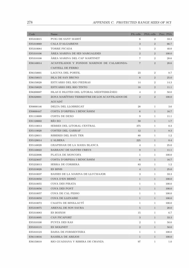
278 APPENDIX C. PROTECTED RANGE SIZES OF SCI
Code Name PA cells PSA cells Perc. PSA
ES5310015 PUIG DE SANT MARTI 6 2 33.3
ES5310069 CALA D’ALGAIRENS 3 2 66.7
ES5310084 TORRE PICADA 5 2 40.0
ES5310106 AREA MARINA DE SES MARGALIDES 2 2 100.0
ES5310108 AREA MARINA DEL CAP MARTINET 7 2 28.6
ES6140014 ACANTILADOS Y FONDOS MARINOS DE CALAHONDA-
CASTELL DE FERRO
7 2 28.6
ES6150001 LAGUNA DEL PORTIL 23 2 8.7
ES6150015 ISLA DE SAN BRUNO 8 2 25.0
ES6150028 ESTUARIO DEL RIO PIEDRAS 14 2 14.3
ES6150029 ESTUARIO DEL RIO TINTO 18 2 11.1
ES6200007 ISLAS E ISLOTES DEL LITORAL MEDITERRANEO 4 2 50.0
ES6320001 ZONA MARITIMO TERRESTRE DE LOS ACANTILADOS DE
AGUADU
2 2 100.0
ES0000146 DELTA DEL LLOBREGAT 28 1 3.6
ES0000447 COSTA D’ORPESA I BENICASSIM 6 1 16.7
ES1110009 COSTA DE DEXO 9 1 11.1
ES1120002 RIO EO 59 1 1.7
ES5110013 SERRES DEL LITORAL CENTRAL 375 1 0.3
ES5110020 COSTES DEL GARRAF 12 1 8.3
ES5120011 RIBERES DEL BAIX TER 80 1 1.2
ES5120014 L’ALBERA 225 1 0.4
ES5140020 GRAPISSAR DE LA MASIA BLANCA 4 1 25.0
ES5140022 BARRANC DE SANTES CREUS 9 1 11.1
ES5222006 PLATJA DE MONCOFA 1 1 100.0
ES5223037 COSTA D’ORPESA I BENICASSIM 6 1 16.7
ES5233013 SERRA DE CORBERA 83 1 1.2
ES5310028 ES BINIS 4 1 25.0
ES5310037 BASSES DE LA MARINA DE LLUCMAJOR 3 1 33.3
ES5310050 COVA D’EN BESSO 1 1 100.0
ES5310055 COVA DES PIRATA 1 1 100.0
ES5310056 COVA DES PONT 1 1 100.0
ES5310057 COVA DE CAL PESSO 1 1 100.0
ES5310059 COVA DE LLENAIRE 1 1 100.0
ES5310072 CALETA DE BINILLAUTI 1 1 100.0
ES5310075 ARENAL DE SON SAURA 5 1 20.0
ES5310083 ES BOIXOS 15 1 6.7
ES5310095 CAN PICAFORT 3 1 33.3
ES5310100 PUNTA DES RAS 2 1 50.0
ES5310115 ES MOLINET 2 1 50.0
ES5310123 BASSA DE FORMENTERA 1 1 100.0
ES6110016 RAMBLA DE AREJOS 1 1 100.0
ES6150018 RIO GUADIANA Y RIBERA DE CHANZA 97 1 1.0

279
Code Name PA cells PSA cells Perc. PSA
SPAIN TOTAL: 12310 2363 19.2
FRANCE
FR9400574 PORTO/SCANDOLA/REVELLATA/CALVI/CALANCHES
DE PIANA (ZONE TERRESTRE ET MARINE)
202 53 26.2
FR9101440 COMPLEXE LAGUNAIRE DE BAGES-SIGEAN 106 43 40.6
FR9112007 ETANGS DU NARBONNAIS 142 43 30.3
FR9410023 GOLFE DE PORTO ET PRESQU’ILE DE SCANDOLA 181 41 22.7
FR9301613 RADE D’HYERES 141 33 23.4
FR9310020 ILES D’HYERES 130 29 22.3
FR9101463 COMPLEXE LAGUNAIRE DE SALSES 89 27 30.3
FR9112005 COMPLEXE LAGUNAIRE DE SALSES-LEUCATE 85 27 31.8
FR9400570 AGRIATES 151 27 17.9
FR9402013 PLATEAU DU CAP CORSE 40 24 60.0
FR9412009 PLATEAU DU CAP CORSE 32 20 62.5
FR9402017 GOLFE D’AJACCIO 66 16 24.2
FR9410096 ILES SANGUINAIRES, GOLFE D’AJACCIO 66 16 24.2
FR9412010 CAPU ROSSU , SCANDOLA, REVELLATA, CALVI 40 15 37.5
FR9400592 VENTILEGNE-LA TRINITE DE BONIFACIO-FAZZIO 46 14 30.4
FR9400568 CAP CORSE NORD ET ILE FINOCCHIAROLA, GIRAGLIA
ET CAPENSE (COTE DE MACINAGGIO A C
47 13 27.7
FR9410098 URBINO 41 13 31.7
FR9410097 ILES FINOCCHIAROLA ET COTE NORD 27 11 40.7
FR9402001 CAMPOMORO-SENETOSA 40 10 25.0
FR9402015 BOUCHES DE BONIFACIO, ILES DES MOINES 87 10 11.5
FR9402018 CAP ROSSU, SCANDOLA, POINTE DE LA REVELETTA,
CANYON DE CALVI
25 10 40.0
FR9410021 ILES LAVEZZI, BOUCHES DE BONIFACIO 111 10 9.0
FR9312008 SALINS D’HYERES ET DES PESQUIERS 21 9 42.9
FR9400580 MARAIS DEL SALE, ZONES HUMIDES PERIPHERIQUES ET
FORET LITTORALE DE PINIA
22 9 40.9
FR9101481 COTE ROCHEUSE DES ALBERES 28 8 28.6
FR9402016 POINTE DE SENETOSA ET PROLONGEMENTS 35 7 20.0
FR9400571 ETANG DE BIGUGLIA 37 6 16.2
FR9101441 COMPLEXE LAGUNAIRE DE LAPALME 31 5 16.1
FR9112006 ETANG DE LAPALME 55 5 9.1
FR9112034 CAP BEAR- CAP CERBERE 16 5 31.2
FR9301592 CAMARGUE 884 5 0.6
FR9310019 CAMARGUE 899 5 0.6
FR9400572 MUCCHIATANA 9 5 55.6
FR9400593 ROCCAPINA-ORTOLO 24 5 20.8
FR9410101 ETANG DE BIGUGLIA 35 5 14.3
FR9301590 LE RHONE AVAL 318 4 1.3
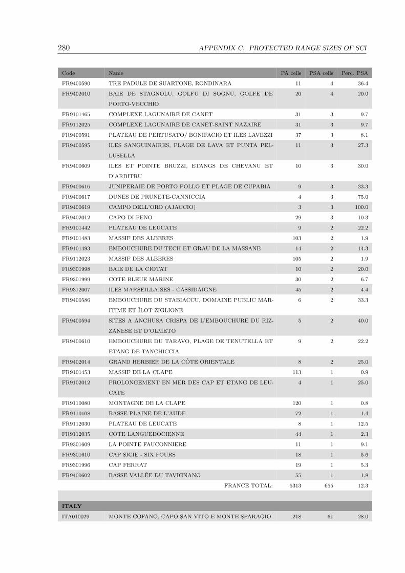
280 APPENDIX C. PROTECTED RANGE SIZES OF SCI
Code Name PA cells PSA cells Perc. PSA
FR9400590 TRE PADULE DE SUARTONE, RONDINARA 11 4 36.4
FR9402010 BAIE DE STAGNOLU, GOLFU DI SOGNU, GOLFE DE
PORTO-VECCHIO
20 4 20.0
FR9101465 COMPLEXE LAGUNAIRE DE CANET 31 3 9.7
FR9112025 COMPLEXE LAGUNAIRE DE CANET-SAINT NAZAIRE 31 3 9.7
FR9400591 PLATEAU DE PERTUSATO/ BONIFACIO ET ILES LAVEZZI 37 3 8.1
FR9400595 ILES SANGUINAIRES, PLAGE DE LAVA ET PUNTA PEL-
LUSELLA
11 3 27.3
FR9400609 ILES ET POINTE BRUZZI, ETANGS DE CHEVANU ET
D’ARBITRU
10 3 30.0
FR9400616 JUNIPERAIE DE PORTO POLLO ET PLAGE DE CUPABIA 9 3 33.3
FR9400617 DUNES DE PRUNETE-CANNICCIA 4 3 75.0
FR9400619 CAMPO DELL’ORO (AJACCIO) 3 3 100.0
FR9402012 CAPO DI FENO 29 3 10.3
FR9101442 PLATEAU DE LEUCATE 9 2 22.2
FR9101483 MASSIF DES ALBERES 103 2 1.9
FR9101493 EMBOUCHURE DU TECH ET GRAU DE LA MASSANE 14 2 14.3
FR9112023 MASSIF DES ALBERES 105 2 1.9
FR9301998 BAIE DE LA CIOTAT 10 2 20.0
FR9301999 COTE BLEUE MARINE 30 2 6.7
FR9312007 ILES MARSEILLAISES - CASSIDAIGNE 45 2 4.4
FR9400586 EMBOUCHURE DU STABIACCU, DOMAINE PUBLIC MAR-
ITIME ET ILOT ZIGLIONE
6 2 33.3
FR9400594 SITES A ANCHUSA CRISPA DE L’EMBOUCHURE DU RIZ-
ZANESE ET D’OLMETO
5 2 40.0
FR9400610 EMBOUCHURE DU TARAVO, PLAGE DE TENUTELLA ET
ETANG DE TANCHICCIA
9 2 22.2
FR9402014 GRAND HERBIER DE LA COTE ORIENTALE 8 2 25.0
FR9101453 MASSIF DE LA CLAPE 113 1 0.9
FR9102012 PROLONGEMENT EN MER DES CAP ET ETANG DE LEU-
CATE
4 1 25.0
FR9110080 MONTAGNE DE LA CLAPE 120 1 0.8
FR9110108 BASSE PLAINE DE L’AUDE 72 1 1.4
FR9112030 PLATEAU DE LEUCATE 8 1 12.5
FR9112035 COTE LANGUEDOCIENNE 44 1 2.3
FR9301609 LA POINTE FAUCONNIERE 11 1 9.1
FR9301610 CAP SICIE - SIX FOURS 18 1 5.6
FR9301996 CAP FERRAT 19 1 5.3
FR9400602 BASSE VALLEE DU TAVIGNANO 55 1 1.8
FRANCE TOTAL: 5313 655 12.3
ITALY
ITA010029 MONTE COFANO, CAPO SAN VITO E MONTE SPARAGIO 218 61 28.0
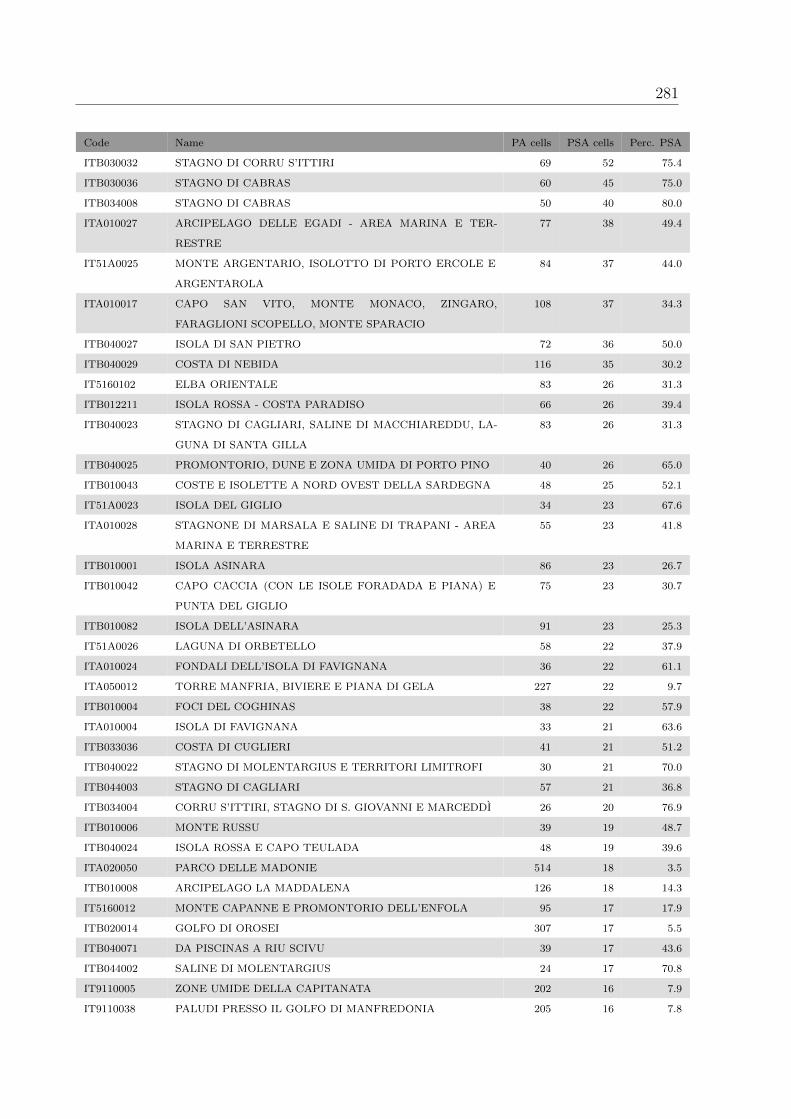
281
Code Name PA cells PSA cells Perc. PSA
ITB030032 STAGNO DI CORRU S’ITTIRI 69 52 75.4
ITB030036 STAGNO DI CABRAS 60 45 75.0
ITB034008 STAGNO DI CABRAS 50 40 80.0
ITA010027 ARCIPELAGO DELLE EGADI - AREA MARINA E TER-
RESTRE
77 38 49.4
IT51A0025 MONTE ARGENTARIO, ISOLOTTO DI PORTO ERCOLE E
ARGENTAROLA
84 37 44.0
ITA010017 CAPO SAN VITO, MONTE MONACO, ZINGARO,
FARAGLIONI SCOPELLO, MONTE SPARACIO
108 37 34.3
ITB040027 ISOLA DI SAN PIETRO 72 36 50.0
ITB040029 COSTA DI NEBIDA 116 35 30.2
IT5160102 ELBA ORIENTALE 83 26 31.3
ITB012211 ISOLA ROSSA - COSTA PARADISO 66 26 39.4
ITB040023 STAGNO DI CAGLIARI, SALINE DI MACCHIAREDDU, LA-
GUNA DI SANTA GILLA
83 26 31.3
ITB040025 PROMONTORIO, DUNE E ZONA UMIDA DI PORTO PINO 40 26 65.0
ITB010043 COSTE E ISOLETTE A NORD OVEST DELLA SARDEGNA 48 25 52.1
IT51A0023 ISOLA DEL GIGLIO 34 23 67.6
ITA010028 STAGNONE DI MARSALA E SALINE DI TRAPANI - AREA
MARINA E TERRESTRE
55 23 41.8
ITB010001 ISOLA ASINARA 86 23 26.7
ITB010042 CAPO CACCIA (CON LE ISOLE FORADADA E PIANA) E
PUNTA DEL GIGLIO
75 23 30.7
ITB010082 ISOLA DELL’ASINARA 91 23 25.3
IT51A0026 LAGUNA DI ORBETELLO 58 22 37.9
ITA010024 FONDALI DELL’ISOLA DI FAVIGNANA 36 22 61.1
ITA050012 TORRE MANFRIA, BIVIERE E PIANA DI GELA 227 22 9.7
ITB010004 FOCI DEL COGHINAS 38 22 57.9
ITA010004 ISOLA DI FAVIGNANA 33 21 63.6
ITB033036 COSTA DI CUGLIERI 41 21 51.2
ITB040022 STAGNO DI MOLENTARGIUS E TERRITORI LIMITROFI 30 21 70.0
ITB044003 STAGNO DI CAGLIARI 57 21 36.8
ITB034004 CORRU S’ITTIRI, STAGNO DI S. GIOVANNI E MARCEDDI 26 20 76.9
ITB010006 MONTE RUSSU 39 19 48.7
ITB040024 ISOLA ROSSA E CAPO TEULADA 48 19 39.6
ITA020050 PARCO DELLE MADONIE 514 18 3.5
ITB010008 ARCIPELAGO LA MADDALENA 126 18 14.3
IT5160012 MONTE CAPANNE E PROMONTORIO DELL’ENFOLA 95 17 17.9
ITB020014 GOLFO DI OROSEI 307 17 5.5
ITB040071 DA PISCINAS A RIU SCIVU 39 17 43.6
ITB044002 SALINE DI MOLENTARGIUS 24 17 70.8
IT9110005 ZONE UMIDE DELLA CAPITANATA 202 16 7.9
IT9110038 PALUDI PRESSO IL GOLFO DI MANFREDONIA 205 16 7.8

282 APPENDIX C. PROTECTED RANGE SIZES OF SCI
Code Name PA cells PSA cells Perc. PSA
ITA070001 FOCE DEL FIUME SIMETO E LAGO GORNALUNGA 37 16 43.2
ITB010003 STAGNO E GINEPRETO DI PLATAMONA 28 16 57.1
ITB020041 ENTROTERRA E ZONA COSTIERA TRA BOSA, CAPO
MARARGIU E PORTO TANGONE
337 16 4.7
ITA070029 BIVIERE DI LENTINI, TRATTO MEDIANO E FOCE DEL FI-
UME SIMETO E AREA ANTISTANTE LA
94 15 16.0
ITB043035 COSTA E ENTROTERRA TRA PUNTA CANNONI E PUNTA
DELLE OCHE - ISOLA DI SAN PIETRO
28 15 53.6
ITB032228 IS ARENAS 20 14 70.0
ITB013044 CAPO CACCIA 51 13 25.5
ITB020012 BERCHIDA E BIDDEROSA 37 13 35.1
ITB040031 MONTE ARCUENTU E RIO PISCINAS 138 13 9.4
ITA010007 SALINE DI TRAPANI 25 12 48.0
ITB010002 STAGNO DI PILO E DI CASARACCIO 28 12 42.9
ITB011155 LAGO DI BARATZ - PORTO FERRO 25 12 48.0
ITB013019 ISOLE DEL NORD - EST TRA CAPO CERASO E STAGNO
DI SAN TEODORO
67 12 17.9
ITB020015 AREA DEL MONTE FERRU DI TERTENIA 41 12 29.3
ITB030034 STAGNO DI MISTRAS DI ORISTANO 25 12 48.0
ITB040030 CAPO PECORA 55 12 21.8
IT5160014 ISOLA DI MONTECRISTO 20 11 55.0
IT5160017 ISOLA DI MONTECRISTO E FORMICA DI MONTECRISTO
- AREA TERRESTRE E MARINA
20 11 55.0
ITA010002 ISOLA DI MARETTIMO 24 11 45.8
ITA010011 SISTEMA DUNALE CAPO GRANITOLA, PORTO PALO E
FOCE DEL BELICE
31 11 35.5
ITA050001 BIVIERE E MACCONI DI GELA 55 11 20.0
ITA070004 TIMPA DI ACIREALE 13 11 84.6
ITB013012 STAGNO DI PILO, CASARACCIO E SALINE DI STINTINO 24 11 45.8
ITB030035 STAGNO DI SALE ’E PORCUS 15 11 73.3
ITB034007 STAGNO DI SALE E’ PORCUS 14 11 78.6
IT5160013 ISOLA DI PIANOSA 21 10 47.6
IT5160016 ISOLA DI PIANOSA - AREA TERRESTRE E MARINA 22 10 45.5
IT9320302 MARCHESATO E FIUME NETO 809 10 1.2
ITA010005 LAGHETTI DI PREOLA E GORGHI TONDI E SCIARE DI
MAZARA
40 9 22.5
ITA010010 MONTE SAN GIULIANO 20 9 45.0
ITA010015 COMPLESSO MONTI DI CASTELLAMMARE DEL GOLFO
(TP)
44 9 20.5
ITA010031 LAGHETTI DI PREOLA E GORGHI TONDI, SCIARE DI
MAZARA E PANTANO LEONE
42 9 21.4
ITA020018 FOCE DEL FIUME POLLINA E MONTE TARDARA 41 9 22.0

283
Code Name PA cells PSA cells Perc. PSA
ITA040003 FOCE DEL MAGAZZOLO, FOCE DEL PLATANI, CAPO
BIANCO, TORRE SALSA
34 9 26.5
ITB023037 COSTA E ENTROTERRA DI BOSA, SUNI E MONTRESTA 126 9 7.1
ITB030016 STAGNO DI S’ENA ARRUBIA E TERRITORI LIMITROFI 9 9 100.0
ITB040017 STAGNI DI MURTAS E S’ACQUA DURCI 15 9 60.0
ITB042226 STAGNO DI PORTO BOTTE 18 9 50.0
ITB043032 ISOLA DI SANT’ANTIOCO, CAPO SPERONE 23 9 39.1
IT9130004 MAR PICCOLO 39 8 20.5
IT9130006 PINETE DELL’ARCO IONICO 67 8 11.9
IT9320095 FOCE NETO 15 8 53.3
ITA010016 MONTE COFANO E LITORALE 13 8 61.5
ITA010021 SALINE DI MARSALA 14 8 57.1
ITA050011 TORRE MANFRIA 24 8 33.3
ITB022214 LIDO DI ORRI 9 8 88.9
ITB034006 STAGNO DI MISTRAS 16 8 50.0
ITB042250 DA IS ARENAS A TONNARA (MARINA DI GONNESA) 8 8 100.0
ITA010006 PALUDI DI CAPO FETO E MARGI SPANO 15 7 46.7
ITA040010 LITORALE DI PALMA DI MONTECHIARO 19 7 36.8
ITA090008 CAPO MURRO DI PORCO, PENISOLA DELLA MAD-
DALENA E GROTTA PELLEGRINO
9 7 77.8
ITB032219 SASSU - CIRRAS 7 7 100.0
ITB042247 IS COMPINXIUS - CAMPO DUNALE DI BUGERRU - POR-
TIXEDDU
11 7 63.6
IT9110015 DUNA E LAGO DI LESINA - FOCE DEL FORTORE 148 6 4.1
ITA010001 ISOLE DELLO STAGNONE DI MARSALA 19 6 31.6
ITA010025 FONDALI DEL GOLFO DI CUSTONACI 11 6 54.5
ITA020038 SUGHERETE DI CONTRADA SERRADAINO 12 6 50.0
ITA090006 SALINE DI SIRACUSA E FIUME CIANE 13 6 46.2
ITA090026 FONDALI DI BRUCOLI - AGNONE 12 6 50.0
ITA090029 PANTANI DELLA SICILIA SUD-ORIENTALE, MORGHELLA,
DI MARZAMEMI, DI PUNTA PILIERI E
80 6 7.5
ITB034001 STAGNO DI S’ENA ARRUBIA 6 6 100.0
ITB040021 COSTA DI CAGLIARI 44 6 13.6
ITB043025 STAGNI DI COLOSTRAI 36 6 16.7
ITA010003 ISOLA DI LEVANZO 12 5 41.7
ITA010026 FONDALI DELL’ISOLA DELLO STAGNONE DI MARSALA 16 5 31.2
ITA030043 MONTI NEBRODI 819 5 0.6
ITA070028 FONDALI DI ACICASTELLO (ISOLA LACHEA - CICLOPI) 7 5 71.4
ITA090002 VENDICARI 30 5 16.7
ITA090007 CAVA GRANDE DEL CASSIBILE, CAVA CINQUE PORTE,
CAVA E BOSCO DI BAULI
89 5 5.6
ITB010011 STAGNO DI SAN TEODORO 15 5 33.3
ITB020013 PALUDE DI OSALLA 23 5 21.7

284 APPENDIX C. PROTECTED RANGE SIZES OF SCI
Code Name PA cells PSA cells Perc. PSA
ITB030038 STAGNO DI PUTZU IDU (SALINA MANNA E PAULI
MARIGOSA)
10 5 50.0
ITB030080 ISOLA DI MAL DI VENTRE E CATALANO 18 5 27.8
ITB032229 IS ARENAS S’ACQUA E S’OLLASTU 7 5 71.4
ITB042218 STAGNO DI PISCINNI 8 5 62.5
ITB042220 SERRA IS TRES PORTUS (SANT’ANTIOCO) 7 5 71.4
IT51A0028 DUNA DI FENIGLIA 13 4 30.8
IT6010018 LITORALE A NORD OVEST DELLE FOCI DEL FIORA 12 4 33.3
IT6010027 LITORALE TRA TARQUINIA E MONTALTO DI CASTRO 11 4 36.4
IT9150015 LITORALE DI GALLIPOLI E ISOLA S. ANDREA 18 4 22.2
IT9310304 ALTO IONIO COSENTINO 381 4 1.0
ITA030044 ARCIPELAGO DELLE EOLIE - AREA MARINA E TER-
RESTRE
197 4 2.0
ITA090027 FONDALI DI VENDICARI 10 4 40.0
ITB040028 PUNTA S’ALIGA 11 4 36.4
ITB042223 STAGNO DI SANTA CATERINA 11 4 36.4
ITB042225 IS PRUINIS 6 4 66.7
IT5160006 ISOLA DI CAPRAIA 33 3 9.1
IT5160007 ISOLA DI CAPRAIA - AREA TERRESTRE E MARINA 32 3 9.4
IT5160009 PROMONTORIO DI PIOMBINO E MONTE MASSONCELLO 16 3 18.8
IT51A0011 PADULE DI DIACCIA BOTRONA 24 3 12.5
IT51A0012 TOMBOLO DA CASTIGLION DELLA PESCAIA A MARINA
DI GROSSETO
16 3 18.8
IT51A0013 PADULE DELLA TRAPPOLA, BOCCA D’OMBRONE 11 3 27.3
IT51A0016 MONTI DELL’UCCELLINA 65 3 4.6
IT51A0024 ISOLA DI GIANNUTRI 10 3 30.0
IT51A0031 LAGO DI BURANO 7 3 42.9
IT51A0033 LAGO DI BURANO 12 3 25.0
IT51A0037 ISOLA DI GIANNUTRI - AREA TERRESTRE E MARINA 10 3 30.0
IT6030005 COMPRENSORIO TOLFETANO-CERITE-MANZIATE 770 3 0.4
IT9110037 LAGHI DI LESINA E VARANO 212 3 1.4
IT9140002 LITORALE BRINDISINO 18 3 16.7
IT9150009 LITORALE DI UGENTO 27 3 11.1
IT9320104 COLLINE DI CROTONE 12 3 25.0
ITA020001 ROCCA DI CEFALU 3 3 100.0
ITA020002 BOSCHI DI GIBILMANNA E CEFALU 44 3 6.8
ITA020014 MONTE PELLEGRINO 15 3 20.0
ITA090014 SALINE DI AUGUSTA 3 3 100.0
ITB030037 STAGNO DI SANTA GIUSTA 20 3 15.0
ITB040018 FOCE DEL FLUMENDOSA - SA PRAIA 13 3 23.1
ITB042208 TRA POGGIO LA SALINA E PUNTA MAGGIORE 3 3 100.0
ITB042210 PUNTA GIUNCHERA 3 3 100.0
IT51A0008 MONTE D’ALMA 79 2 2.5
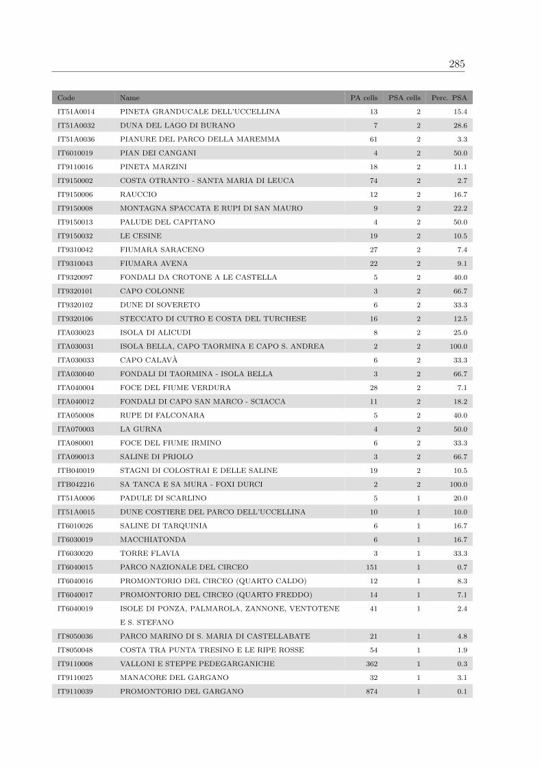
285
Code Name PA cells PSA cells Perc. PSA
IT51A0014 PINETA GRANDUCALE DELL’UCCELLINA 13 2 15.4
IT51A0032 DUNA DEL LAGO DI BURANO 7 2 28.6
IT51A0036 PIANURE DEL PARCO DELLA MAREMMA 61 2 3.3
IT6010019 PIAN DEI CANGANI 4 2 50.0
IT9110016 PINETA MARZINI 18 2 11.1
IT9150002 COSTA OTRANTO - SANTA MARIA DI LEUCA 74 2 2.7
IT9150006 RAUCCIO 12 2 16.7
IT9150008 MONTAGNA SPACCATA E RUPI DI SAN MAURO 9 2 22.2
IT9150013 PALUDE DEL CAPITANO 4 2 50.0
IT9150032 LE CESINE 19 2 10.5
IT9310042 FIUMARA SARACENO 27 2 7.4
IT9310043 FIUMARA AVENA 22 2 9.1
IT9320097 FONDALI DA CROTONE A LE CASTELLA 5 2 40.0
IT9320101 CAPO COLONNE 3 2 66.7
IT9320102 DUNE DI SOVERETO 6 2 33.3
IT9320106 STECCATO DI CUTRO E COSTA DEL TURCHESE 16 2 12.5
ITA030023 ISOLA DI ALICUDI 8 2 25.0
ITA030031 ISOLA BELLA, CAPO TAORMINA E CAPO S. ANDREA 2 2 100.0
ITA030033 CAPO CALAVA 6 2 33.3
ITA030040 FONDALI DI TAORMINA - ISOLA BELLA 3 2 66.7
ITA040004 FOCE DEL FIUME VERDURA 28 2 7.1
ITA040012 FONDALI DI CAPO SAN MARCO - SCIACCA 11 2 18.2
ITA050008 RUPE DI FALCONARA 5 2 40.0
ITA070003 LA GURNA 4 2 50.0
ITA080001 FOCE DEL FIUME IRMINO 6 2 33.3
ITA090013 SALINE DI PRIOLO 3 2 66.7
ITB040019 STAGNI DI COLOSTRAI E DELLE SALINE 19 2 10.5
ITB042216 SA TANCA E SA MURA - FOXI DURCI 2 2 100.0
IT51A0006 PADULE DI SCARLINO 5 1 20.0
IT51A0015 DUNE COSTIERE DEL PARCO DELL’UCCELLINA 10 1 10.0
IT6010026 SALINE DI TARQUINIA 6 1 16.7
IT6030019 MACCHIATONDA 6 1 16.7
IT6030020 TORRE FLAVIA 3 1 33.3
IT6040015 PARCO NAZIONALE DEL CIRCEO 151 1 0.7
IT6040016 PROMONTORIO DEL CIRCEO (QUARTO CALDO) 12 1 8.3
IT6040017 PROMONTORIO DEL CIRCEO (QUARTO FREDDO) 14 1 7.1
IT6040019 ISOLE DI PONZA, PALMAROLA, ZANNONE, VENTOTENE
E S. STEFANO
41 1 2.4
IT8050036 PARCO MARINO DI S. MARIA DI CASTELLABATE 21 1 4.8
IT8050048 COSTA TRA PUNTA TRESINO E LE RIPE ROSSE 54 1 1.9
IT9110008 VALLONI E STEPPE PEDEGARGANICHE 362 1 0.3
IT9110025 MANACORE DEL GARGANO 32 1 3.1
IT9110039 PROMONTORIO DEL GARGANO 874 1 0.1
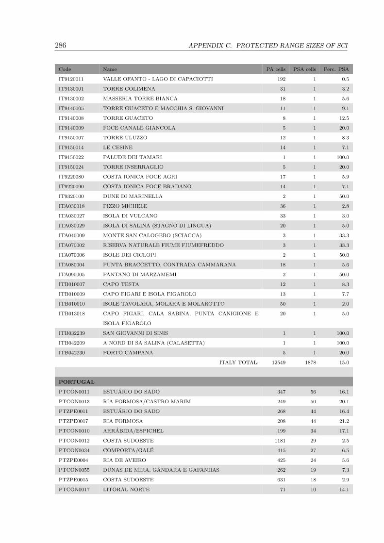
286 APPENDIX C. PROTECTED RANGE SIZES OF SCI
Code Name PA cells PSA cells Perc. PSA
IT9120011 VALLE OFANTO - LAGO DI CAPACIOTTI 192 1 0.5
IT9130001 TORRE COLIMENA 31 1 3.2
IT9130002 MASSERIA TORRE BIANCA 18 1 5.6
IT9140005 TORRE GUACETO E MACCHIA S. GIOVANNI 11 1 9.1
IT9140008 TORRE GUACETO 8 1 12.5
IT9140009 FOCE CANALE GIANCOLA 5 1 20.0
IT9150007 TORRE ULUZZO 12 1 8.3
IT9150014 LE CESINE 14 1 7.1
IT9150022 PALUDE DEI TAMARI 1 1 100.0
IT9150024 TORRE INSERRAGLIO 5 1 20.0
IT9220080 COSTA IONICA FOCE AGRI 17 1 5.9
IT9220090 COSTA IONICA FOCE BRADANO 14 1 7.1
IT9320100 DUNE DI MARINELLA 2 1 50.0
ITA030018 PIZZO MICHELE 36 1 2.8
ITA030027 ISOLA DI VULCANO 33 1 3.0
ITA030029 ISOLA DI SALINA (STAGNO DI LINGUA) 20 1 5.0
ITA040009 MONTE SAN CALOGERO (SCIACCA) 3 1 33.3
ITA070002 RISERVA NATURALE FIUME FIUMEFREDDO 3 1 33.3
ITA070006 ISOLE DEI CICLOPI 2 1 50.0
ITA080004 PUNTA BRACCETTO, CONTRADA CAMMARANA 18 1 5.6
ITA090005 PANTANO DI MARZAMEMI 2 1 50.0
ITB010007 CAPO TESTA 12 1 8.3
ITB010009 CAPO FIGARI E ISOLA FIGAROLO 13 1 7.7
ITB010010 ISOLE TAVOLARA, MOLARA E MOLAROTTO 50 1 2.0
ITB013018 CAPO FIGARI, CALA SABINA, PUNTA CANIGIONE E
ISOLA FIGAROLO
20 1 5.0
ITB032239 SAN GIOVANNI DI SINIS 1 1 100.0
ITB042209 A NORD DI SA SALINA (CALASETTA) 1 1 100.0
ITB042230 PORTO CAMPANA 5 1 20.0
ITALY TOTAL: 12549 1878 15.0
PORTUGAL
PTCON0011 ESTUARIO DO SADO 347 56 16.1
PTCON0013 RIA FORMOSA/CASTRO MARIM 249 50 20.1
PTZPE0011 ESTUARIO DO SADO 268 44 16.4
PTZPE0017 RIA FORMOSA 208 44 21.2
PTCON0010 ARRABIDA/ESPICHEL 199 34 17.1
PTCON0012 COSTA SUDOESTE 1181 29 2.5
PTCON0034 COMPORTA/GALE 415 27 6.5
PTZPE0004 RIA DE AVEIRO 425 24 5.6
PTCON0055 DUNAS DE MIRA, GANDARA E GAFANHAS 262 19 7.3
PTZPE0015 COSTA SUDOESTE 631 18 2.9
PTCON0017 LITORAL NORTE 71 10 14.1

287
Code Name PA cells PSA cells Perc. PSA
PTCON0009 ESTUARIO DO TEJO 385 8 2.1
PTZPE0010 ESTUARIO DO TEJO 395 8 2.0
PTZPE0013 LAGOA DE SANTO ANDRE 25 6 24.0
PTCON0008 SINTRA/CASCAIS 174 5 2.9
PTZPE0014 LAGOA DA SANCHA 5 4 80.0
PTZPE0050 CABO ESPICHEL 21 4 19.0
PTZPE0018 SAPAIS DE CASTRO MARIM 34 3 8.8
PTCON0018 BARRINHA DE ESMORIZ 10 2 20.0
PTCON0056 PENICHE / STa CRUZ 91 1 1.1
PORTUGAL TOTAL: 5396 396 7.3
OVERALL NATURA 2000 TOTAL: 35568 5292 14.9
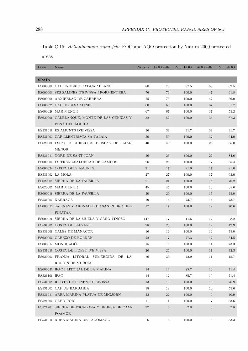
288 APPENDIX C. PROTECTED RANGE SIZES OF SCI
Table C.15: Helianthemum caput-felis EOO and AOO protection by Natura 2000 protected
areas
Code Name PA cells EOO cells Perc. EOO AOO cells Perc. AOO
SPAIN
ES0000081CAP ENDERROCAT-CAP BLANC 80 70 87.5 50 62.5
ES0000084SES SALINES D’EIVISSA I FORMENTERA 76 76 100.0 47 61.8
ES0000083ARXIPELAG DE CABRERA 75 75 100.0 42 56.0
ES0000228CAP DE SES SALINES 60 60 100.0 37 61.7
ES0000260MAR MENOR 67 67 100.0 37 55.2
ES6200001CALBLANQUE, MONTE DE LAS CENIZAS Y
PENA DEL AGUILA
52 52 100.0 35 67.3
ES5310105ES AMUNTS D’EIVISSA 36 33 91.7 33 91.7
ES5310032CAP LLENTRISCA-SA TALAIA 50 50 100.0 32 64.0
ES6200006ESPACIOS ABIERTOS E ISLAS DEL MAR
MENOR
40 40 100.0 26 65.0
ES5310112NORD DE SANT JOAN 26 26 100.0 22 84.6
ES0000037ES TRENC-SALOBRAR DE CAMPOS 26 26 100.0 17 65.4
ES0000241COSTA DELS AMUNTS 21 17 81.0 17 81.0
ES5310024LA MOLA 27 27 100.0 17 63.0
ES6200025SIERRA DE LA FAUSILLA 21 21 100.0 16 76.2
ES6200030MAR MENOR 45 45 100.0 16 35.6
ES0000199SIERRA DE LA FAUSILLA 20 20 100.0 15 75.0
ES5310033XARRACA 19 14 73.7 14 73.7
ES0000175SALINAS Y ARENALES DE SAN PEDRO DEL
PINATAR
17 17 100.0 12 70.6
ES0000264SIERRA DE LA MUELA Y CABO TINOSO 147 17 11.6 12 8.2
ES5310030COSTA DE LLEVANT 28 28 100.0 12 42.9
ES5310098CALES DE MANACOR 16 16 100.0 12 75.0
ES6200024CABEZO DE ROLDAN 22 17 77.3 12 54.5
ES0000145MONDRAGO 15 15 100.0 11 73.3
ES5310104COSTA DE L’OEST D’EIVISSA 26 26 100.0 11 42.3
ES6200029FRANJA LITORAL SUMERGIDA DE LA
REGION DE MURCIA
70 30 42.9 11 15.7
ES0000459IFAC I LITORAL DE LA MARINA 14 12 85.7 10 71.4
ES5211009IFAC 14 12 85.7 10 71.4
ES5310023ILLOTS DE PONENT D’EIVISSA 13 13 100.0 10 76.9
ES5310025CAP DE BARBARIA 18 18 100.0 10 55.6
ES5310111AREA MARINA PLATJA DE MIGJORN 22 22 100.0 9 40.9
ES5213033CABO ROIG 11 11 100.0 7 63.6
ES5212012SIERRA DE ESCALONA Y DEHESA DE CAM-
POAMOR
77 6 7.8 6 7.8
ES5310107AREA MARINA DE TAGOMAGO 6 6 100.0 5 83.3

289
Code Name PA cells EOO cells Perc. EOO AOO cells Perc. AOO
ES0000078ES VEDRA-ES VEDRANELL 6 6 100.0 4 66.7
ES0000464SIERRA ESCALONA Y DEHESA DE CAM-
POAMOR
136 4 2.9 4 2.9
ES5213018PENYA-SEGATS DE LA MARINA 31 5 16.1 4 12.9
ES0000082TAGOMAGO 3 3 100.0 3 100.0
ES5310031PORROIG 3 3 100.0 3 100.0
ES5310034SERRA GROSSA 25 25 100.0 3 12.0
ES5310099PORTOCOLOM 5 5 100.0 3 60.0
ES5310109AREA MARINA DE CALA SAONA 4 4 100.0 3 75.0
ES5310106AREA MARINA DE SES MARGALIDES 2 2 100.0 2 100.0
ES5310108AREA MARINA DEL CAP MARTINET 7 7 100.0 2 28.6
ES6320001ZONA MARITIMO TERRESTRE DE LOS
ACANTILADOS DE AGUADU
2 2 100.0 2 100.0
ES6320002BARRANCO DEL NANO 4 2 50.0 2 50.0
ES0000059LLACUNES DE LA MATA I TORREVIEJA. 60 1 1.7 1 1.7
ES5310037BASSES DE LA MARINA DE LLUCMAJOR 3 3 100.0 1 33.3
ES5310050COVA D’EN BESSO 1 1 100.0 1 100.0
ES5310055COVA DES PIRATA 1 1 100.0 1 100.0
ES5310056COVA DES PONT 1 1 100.0 1 100.0
ES5310100PUNTA DES RAS 2 2 100.0 1 50.0
ES5310123BASSA DE FORMENTERA 1 1 100.0 1 100.0
ES6200048MEDIO MARINO 15 5 33.3 1 6.7
ES0000200ISLA GROSA 1 1 100.0 0 0.0
ES0000214ILLOTS DE TABARCA 12 5 41.7 0 0.0
ES0000242ILLOTS DE SANTA EULARIA, RODONA I ES
CANA
2 2 100.0 0 0.0
ES0000256ISLAS HORMIGAS 1 1 100.0 0 0.0
ES5213024TABARCA 24 5 20.8 0 0.0
ES5310043COVA DELS ASES 1 1 100.0 0 0.0
ES5310048COVA DE SA GUITARRETA 1 1 100.0 0 0.0
ES5310049COVA DES PAS DE VALLGORNERA 1 1 100.0 0 0.0
ES5310061COVA NOVA DE SON LLUIS 1 1 100.0 0 0.0
ES5310110AREA MARINA PLATJA DE TRAMUNTANA 1 1 100.0 0 0.0
ES6200007ISLAS E ISLOTES DEL LITORAL
MEDITERRANEO
4 1 25.0 0 0.0
SPAIN TOTAL: 1618 1088 67.2 676 41.8
ITALY
ITB030038STAGNO DI PUTZU IDU (SALINA MANNA E
PAULI MARIGOSA)
10 4 40.0 2 20.0
ITB030039ISOLA MAL DI VENTRE 6 6 100.0 0 0.0
ITB030080ISOLA DI MAL DI VENTRE E CATALANO 18 9 50.0 0 0.0
ITALY TOTAL: 34 19 55.9 2 5.9

290 APPENDIX C. PROTECTED RANGE SIZES OF SCI
Code Name PA cells EOO cells Perc. EOO AOO cells Perc. AOO
OVERALL NATURA 2000 TOTAL: 1652 1107 67.0 678 41.0

291
Table C.16: Helianthemum caput-felis PSA protection by North African protected areas
Code Type Name PA cells PSA cells Perc. PSA
ALGERIA
26620 UNESCO-MAB Biosphere
Reserve
El Kala 897 31 3.5
9741 National Park El Kala 897 31 3.5
14909 Marine Park El Kala 897 31 3.5
9758 Nature Reserve Macta 207 18 8.7
14904 Breeding Station Boumerdes 100 15 15.0
900574 Wetlands of International
Importance (Ramsar)
Complexe de zones humides de la plaine de
Guerbes-Sanhadja
432 4 0.9
72355 National Park Edough 36 2 5.6
72362 National Park Tigzirt 3 2 66.7
902531 UNESCO-MAB Biosphere
Reserve
Gouraya 18 1 5.6
9747 National Park Gouraya 18 1 5.6
9748 Regional Park Seraidi P 40 1 2.5
72363 National Park Tipaza Chenoua 49 1 2.0
ALGERIA TOTAL: 3594 138 3.8
MOROCCO
29969 National Park Al Hoceima 271 55 20.3
20371 Marine Reserve Bokkoyas 268 54 20.1
11698 Biological Reserve Bokkoyas 268 54 20.1
902715 Wetlands of International
Importance (Ramsar)
Sebkha Bou Areg 55 21 38.2
902704 Wetlands of International
Importance (Ramsar)
Cap des Trois Fourches 26 17 65.4
15099 Nature Reserve Nador 21 3 14.3
168216 UNESCO-MAB Biosphere
Reserve
Arganeraie 20690 2 0.0
MOROCCO TOTAL: 21599 206 1.0
TUNISIA
903084 Wetlands of International
Importance (Ramsar)
Sebkhet Kelbia 238 109 45.8
15185 Wetland Zone of National
Importance
Sebkhet Kelbia 238 109 45.8
903080 Wetlands of International
Importance (Ramsar)
Lagune de Ghar el Melh et DElta de la
Mejerda
71 42 59.2
15188 Nature Reserve Lac Bizerte 90 38 42.2
15182 Nature Reserve Medjerda Estuary 66 36 54.5

292 APPENDIX C. PROTECTED RANGE SIZES OF SCI
Code Type Name PA cells PSA cells Perc. PSA
32554 Wetland Zone of National
Importance
Sebkhet Ariana 43 17 39.5
15194 Wetland Zone of National
Importance
Sebkha Halk el Menzel 20 13 65.0
903087 Wetlands of International
Importance (Ramsar)
Sebkhet Soliman 14 11 78.6
12390 National Park Boukornine 24 9 37.5
903081 Wetlands of International
Importance (Ramsar)
Lagunes du Cap Bon oriental 8 7 87.5
2115 UNESCO-MAB Biosphere
Reserve
Iles Zembra et Zembretta 8 2 25.0
365017 Barcelona Convention Zembra and Zembretta 8 2 25.0
942 National Park Zembra and Zembretta 8 2 25.0
101847 Natural Reserve Grotte de Chauve souris d’El Haouaria 1 1 100.0
15183 Wetland Zone of National
Importance
Sebkhet es Sedjoumi 36 1 2.8
TUNISIA TOTAL: 873 399 45.7
OVERALL NORTH AFRICAN TOTAL: 26066 743 2.9

293
Table C.17: Helianthemum caput-felis EOO and AOO protection by North African
protected areas
Code Type Name PA cells EOO cells Perc. EOO AOO cells Perc. AOO
ALGERIA
365019Barcelona Convention Iles Habibas 4 4 100.0 0 0.0
19571 Marine Nature Reserve Iles Habibas 4 4 100.0 0 0.0
ALGERIA TOTAL: 8 8 100.0 0 0.0
MOROCCO
902704Wetlands of International
Importance (Ramsar)
Cap des Trois Fourches 26 11 42.3 6 23.1
MOROCCO TOTAL: 26 11 42.3 6 23.1
OVERALL NORTH AFRICAN TOTAL: 34 19 55.9 6 17.6

294 APPENDIX C. PROTECTED RANGE SIZES OF SCI
Medicago citrina
Table C.18: Medicago citrina PSA protection by Natura 2000 protected areas
Code Name PA cells PSA cells Perc. PSA
SPAIN
ES0000023 L’ALBUFERA 255 62 24.3
ES0000471 L’ALBUFERA 255 62 24.3
ES0000020 DELTA DE L’EBRE 223 37 16.6
ES0000083 ARXIPELAG DE CABRERA 75 34 45.3
ES0000084 SES SALINES D’EIVISSA I FORMENTERA 76 29 38.2
ES0000081 CAP ENDERROCAT-CAP BLANC 80 28 35.0
ES5310035 AREA MARINA DEL NORD DE MENORCA 34 17 50.0
ES0000073 COSTA BRAVA DE MALLORCA 143 16 11.2
ES0000231 DELS ALOCS A FORNELLS 52 16 30.8
ES0000241 COSTA DELS AMUNTS 21 16 76.2
ES5310105 ES AMUNTS D’EIVISSA 36 15 41.7
ES0000450 MARJAL I ESTANYS D’ALMENARA 32 13 40.6
ES5223007 MARJAL D’ALMENARA 32 13 40.6
ES5310032 CAP LLENTRISCA-SA TALAIA 50 13 26.0
ES5310112 NORD DE SANT JOAN 26 13 50.0
ES0000121 ILLOTS DE BENIDORM I SERRA GELADA 27 12 44.4
ES0000459 IFAC I LITORAL DE LA MARINA 14 12 85.7
ES5211009 IFAC 14 12 85.7
ES5213021 SERRA GELADA I LITORAL DE LA MARINA BAIXA 25 12 48.0
ES5222005 MARJAL DE NULES 19 12 63.2
ES5310030 COSTA DE LLEVANT 28 12 42.9
ES0000074 CAP DE CALA FIGUERA 20 11 55.0
ES0000227 MUNTANYES D’ARTA 129 11 8.5
ES0000228 CAP DE SES SALINES 60 11 18.3
ES0000451 MONTDUVER-MARJAL DE LA SAFOR 149 10 6.7
ES5213018 PENYA-SEGATS DE LA MARINA 31 10 32.3
ES5310023 ILLOTS DE PONENT D’EIVISSA 13 10 76.9
ES5310104 COSTA DE L’OEST D’EIVISSA 26 10 38.5
ES5233030 MARJAL DE LA SAFOR 24 9 37.5
ES5310005 BADIES DE POLLENCA I ALCUDIA 50 9 18.0
ES5310024 LA MOLA 27 9 33.3
ES5310033 XARRACA 19 9 47.4
ES5310111 AREA MARINA PLATJA DE MIGJORN 22 9 40.9
ES0000037 ES TRENC-SALOBRAR DE CAMPOS 26 8 30.8
ES0000229 COSTA NORD DE CIUTADELLA 17 8 47.1
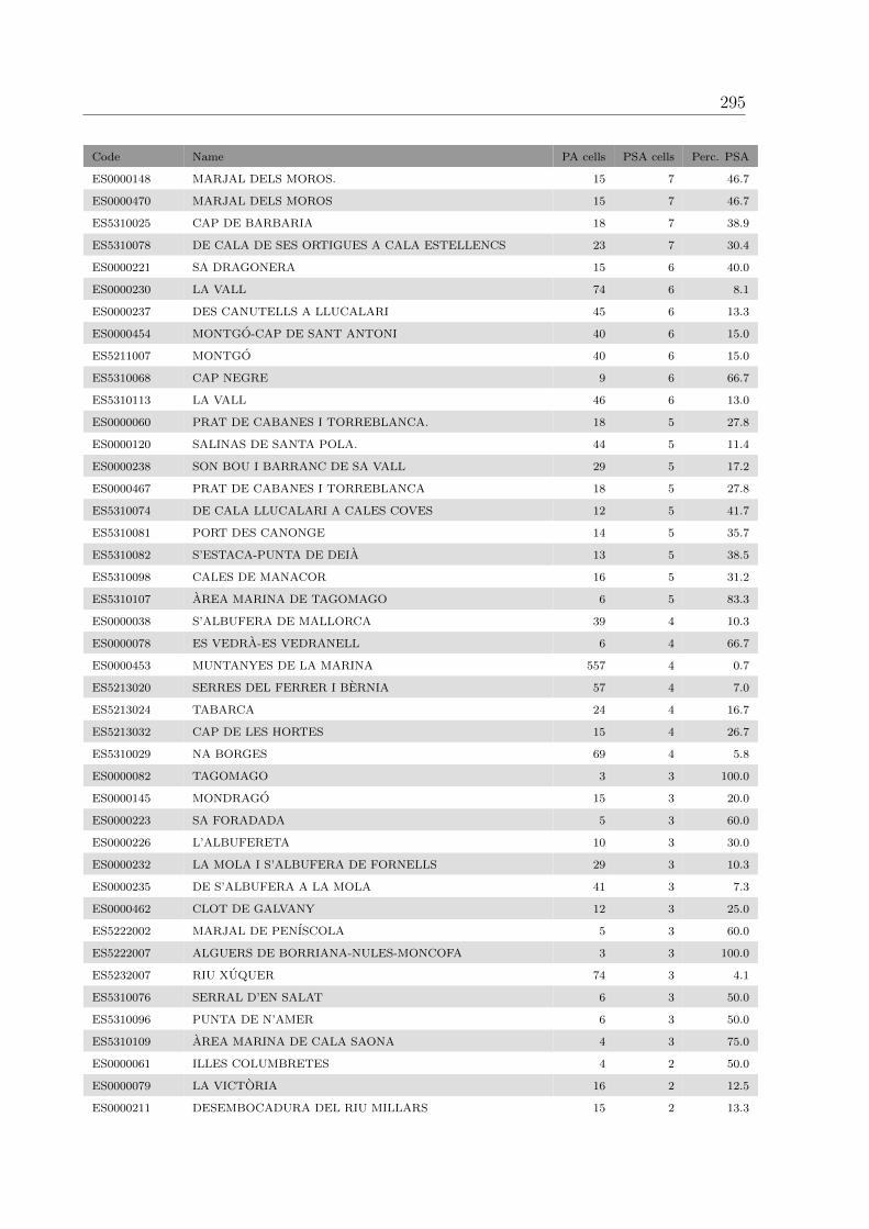
295
Code Name PA cells PSA cells Perc. PSA
ES0000148 MARJAL DELS MOROS. 15 7 46.7
ES0000470 MARJAL DELS MOROS 15 7 46.7
ES5310025 CAP DE BARBARIA 18 7 38.9
ES5310078 DE CALA DE SES ORTIGUES A CALA ESTELLENCS 23 7 30.4
ES0000221 SA DRAGONERA 15 6 40.0
ES0000230 LA VALL 74 6 8.1
ES0000237 DES CANUTELLS A LLUCALARI 45 6 13.3
ES0000454 MONTGO-CAP DE SANT ANTONI 40 6 15.0
ES5211007 MONTGO 40 6 15.0
ES5310068 CAP NEGRE 9 6 66.7
ES5310113 LA VALL 46 6 13.0
ES0000060 PRAT DE CABANES I TORREBLANCA. 18 5 27.8
ES0000120 SALINAS DE SANTA POLA. 44 5 11.4
ES0000238 SON BOU I BARRANC DE SA VALL 29 5 17.2
ES0000467 PRAT DE CABANES I TORREBLANCA 18 5 27.8
ES5310074 DE CALA LLUCALARI A CALES COVES 12 5 41.7
ES5310081 PORT DES CANONGE 14 5 35.7
ES5310082 S’ESTACA-PUNTA DE DEIA 13 5 38.5
ES5310098 CALES DE MANACOR 16 5 31.2
ES5310107 AREA MARINA DE TAGOMAGO 6 5 83.3
ES0000038 S’ALBUFERA DE MALLORCA 39 4 10.3
ES0000078 ES VEDRA-ES VEDRANELL 6 4 66.7
ES0000453 MUNTANYES DE LA MARINA 557 4 0.7
ES5213020 SERRES DEL FERRER I BERNIA 57 4 7.0
ES5213024 TABARCA 24 4 16.7
ES5213032 CAP DE LES HORTES 15 4 26.7
ES5310029 NA BORGES 69 4 5.8
ES0000082 TAGOMAGO 3 3 100.0
ES0000145 MONDRAGO 15 3 20.0
ES0000223 SA FORADADA 5 3 60.0
ES0000226 L’ALBUFERETA 10 3 30.0
ES0000232 LA MOLA I S’ALBUFERA DE FORNELLS 29 3 10.3
ES0000235 DE S’ALBUFERA A LA MOLA 41 3 7.3
ES0000462 CLOT DE GALVANY 12 3 25.0
ES5222002 MARJAL DE PENISCOLA 5 3 60.0
ES5222007 ALGUERS DE BORRIANA-NULES-MONCOFA 3 3 100.0
ES5232007 RIU XUQUER 74 3 4.1
ES5310076 SERRAL D’EN SALAT 6 3 50.0
ES5310096 PUNTA DE N’AMER 6 3 50.0
ES5310109 AREA MARINA DE CALA SAONA 4 3 75.0
ES0000061 ILLES COLUMBRETES 4 2 50.0
ES0000079 LA VICTORIA 16 2 12.5
ES0000211 DESEMBOCADURA DEL RIU MILLARS 15 2 13.3
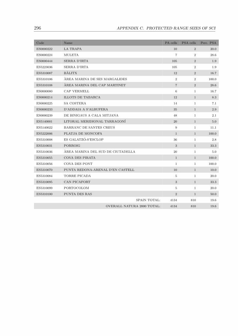
296 APPENDIX C. PROTECTED RANGE SIZES OF SCI
Code Name PA cells PSA cells Perc. PSA
ES0000222 LA TRAPA 10 2 20.0
ES0000224 MULETA 7 2 28.6
ES0000444 SERRA D’IRTA 105 2 1.9
ES5223036 SERRA D’IRTA 105 2 1.9
ES5310087 BALITX 12 2 16.7
ES5310106 AREA MARINA DE SES MARGALIDES 2 2 100.0
ES5310108 AREA MARINA DEL CAP MARTINET 7 2 28.6
ES0000080 CAP VERMELL 6 1 16.7
ES0000214 ILLOTS DE TABARCA 12 1 8.3
ES0000225 SA COSTERA 14 1 7.1
ES0000233 D’ADDAIA A S’ALBUFERA 35 1 2.9
ES0000239 DE BINIGAUS A CALA MITJANA 48 1 2.1
ES5140001 LITORAL MERIDIONAL TARRAGONI 20 1 5.0
ES5140022 BARRANC DE SANTES CREUS 9 1 11.1
ES5222006 PLATJA DE MONCOFA 1 1 100.0
ES5310008 ES GALATZO-S’ESCLOP 36 1 2.8
ES5310031 PORROIG 3 1 33.3
ES5310036 AREA MARINA DEL SUD DE CIUTADELLA 20 1 5.0
ES5310055 COVA DES PIRATA 1 1 100.0
ES5310056 COVA DES PONT 1 1 100.0
ES5310070 PUNTA REDONA-ARENAL D’EN CASTELL 10 1 10.0
ES5310084 TORRE PICADA 5 1 20.0
ES5310095 CAN PICAFORT 3 1 33.3
ES5310099 PORTOCOLOM 5 1 20.0
ES5310100 PUNTA DES RAS 2 1 50.0
SPAIN TOTAL: 4134 810 19.6
OVERALL NATURA 2000 TOTAL: 4134 810 19.6

297
Table C.19: Medicago citrina EOO and AOO protection by Natura 2000 protected areas
Code Name PA cells EOO cells Perc. EOO AOO cells Perc. AOO
SPAIN
ES0000241COSTA DELS AMUNTS 21 21 100.0 16 76.2
ES5310105ES AMUNTS D’EIVISSA 36 36 100.0 15 41.7
ES5310112NORD DE SANT JOAN 26 26 100.0 13 50.0
ES5310032CAP LLENTRISCA-SA TALAIA 50 45 90.0 12 24.0
ES5310023ILLOTS DE PONENT D’EIVISSA 13 13 100.0 10 76.9
ES5310104COSTA DE L’OEST D’EIVISSA 26 22 84.6 10 38.5
ES5310033XARRACA 19 19 100.0 9 47.4
ES0000083ARXIPELAG DE CABRERA 75 15 20.0 7 9.3
ES5310107AREA MARINA DE TAGOMAGO 6 6 100.0 5 83.3
ES0000082TAGOMAGO 3 3 100.0 3 100.0
ES0000061ILLES COLUMBRETES 4 4 100.0 2 50.0
ES5310106AREA MARINA DE SES MARGALIDES 2 2 100.0 2 100.0
ES5310108AREA MARINA DEL CAP MARTINET 7 7 100.0 2 28.6
ES0000078ES VEDRA-ES VEDRANELL 6 2 33.3 1 16.7
ES0000084SES SALINES D’EIVISSA I FORMENTERA 76 2 2.6 1 1.3
ES0000454MONTGO-CAP DE SANT ANTONI 40 1 2.5 1 2.5
ES5211007MONTGO 40 1 2.5 1 2.5
ES5310031PORROIG 3 2 66.7 1 33.3
ES0000242ILLOTS DE SANTA EULARIA, RODONA I ES
CANA
2 2 100.0 0 0.0
ES5310034SERRA GROSSA 25 25 100.0 0 0.0
SPAIN TOTAL: 480 254 52.9 111 23.1
OVERALL NATURA 2000 TOTAL: 480 254 52.9 111 23.1
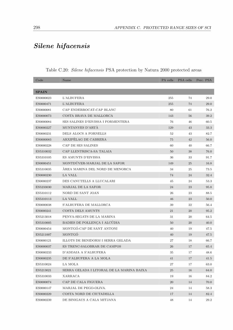
298 APPENDIX C. PROTECTED RANGE SIZES OF SCI
Silene hifacensis
Table C.20: Silene hifacensis PSA protection by Natura 2000 protected areas
Code Name PA cells PSA cells Perc. PSA
SPAIN
ES0000023 L’ALBUFERA 255 74 29.0
ES0000471 L’ALBUFERA 255 74 29.0
ES0000081 CAP ENDERROCAT-CAP BLANC 80 61 76.2
ES0000073 COSTA BRAVA DE MALLORCA 143 56 39.2
ES0000084 SES SALINES D’EIVISSA I FORMENTERA 76 46 60.5
ES0000227 MUNTANYES D’ARTA 129 43 33.3
ES0000231 DELS ALOCS A FORNELLS 52 43 82.7
ES0000083 ARXIPELAG DE CABRERA 75 42 56.0
ES0000228 CAP DE SES SALINES 60 40 66.7
ES5310032 CAP LLENTRISCA-SA TALAIA 50 38 76.0
ES5310105 ES AMUNTS D’EIVISSA 36 33 91.7
ES0000451 MONTDUVER-MARJAL DE LA SAFOR 149 25 16.8
ES5310035 AREA MARINA DEL NORD DE MENORCA 34 25 73.5
ES0000230 LA VALL 74 24 32.4
ES0000237 DES CANUTELLS A LLUCALARI 45 24 53.3
ES5233030 MARJAL DE LA SAFOR 24 23 95.8
ES5310112 NORD DE SANT JOAN 26 23 88.5
ES5310113 LA VALL 46 23 50.0
ES0000038 S’ALBUFERA DE MALLORCA 39 22 56.4
ES0000241 COSTA DELS AMUNTS 21 20 95.2
ES5213018 PENYA-SEGATS DE LA MARINA 31 20 64.5
ES5310005 BADIES DE POLLENCA I ALCUDIA 50 20 40.0
ES0000454 MONTGO-CAP DE SANT ANTONI 40 19 47.5
ES5211007 MONTGO 40 19 47.5
ES0000121 ILLOTS DE BENIDORM I SERRA GELADA 27 18 66.7
ES0000037 ES TRENC-SALOBRAR DE CAMPOS 26 17 65.4
ES0000233 D’ADDAIA A S’ALBUFERA 35 17 48.6
ES0000235 DE S’ALBUFERA A LA MOLA 41 17 41.5
ES5310024 LA MOLA 27 17 63.0
ES5213021 SERRA GELADA I LITORAL DE LA MARINA BAIXA 25 16 64.0
ES5310033 XARRACA 19 16 84.2
ES0000074 CAP DE CALA FIGUERA 20 14 70.0
ES0000147 MARJAL DE PEGO-OLIVA. 24 14 58.3
ES0000229 COSTA NORD DE CIUTADELLA 17 14 82.4
ES0000239 DE BINIGAUS A CALA MITJANA 48 14 29.2

299
Code Name PA cells PSA cells Perc. PSA
ES0000443 SUD DE CIUTADELLA 38 14 36.8
ES0000145 MONDRAGO 15 13 86.7
ES0000232 LA MOLA I S’ALBUFERA DE FORNELLS 29 13 44.8
ES0000238 SON BOU I BARRANC DE SA VALL 29 13 44.8
ES5310029 NA BORGES 69 13 18.8
ES0000240 COSTA SUD DE CIUTADELLA 25 12 48.0
ES0000453 MUNTANYES DE LA MARINA 557 12 2.2
ES0000459 IFAC I LITORAL DE LA MARINA 14 12 85.7
ES5211009 IFAC 14 12 85.7
ES5310030 COSTA DE LLEVANT 28 12 42.9
ES5310098 CALES DE MANACOR 16 12 75.0
ES0000079 LA VICTORIA 16 11 68.8
ES0000234 S’ALBUFERA DES GRAU 31 11 35.5
ES0000450 MARJAL I ESTANYS D’ALMENARA 32 11 34.4
ES5223007 MARJAL D’ALMENARA 32 11 34.4
ES5310104 COSTA DE L’OEST D’EIVISSA 26 11 42.3
ES5310023 ILLOTS DE PONENT D’EIVISSA 13 10 76.9
ES5310025 CAP DE BARBARIA 18 10 55.6
ES0000148 MARJAL DELS MOROS. 15 9 60.0
ES0000226 L’ALBUFERETA 10 9 90.0
ES0000470 MARJAL DELS MOROS 15 9 60.0
ES5222005 MARJAL DE NULES 19 9 47.4
ES5310068 CAP NEGRE 9 9 100.0
ES5310111 AREA MARINA PLATJA DE MIGJORN 22 9 40.9
ES5213020 SERRES DEL FERRER I BERNIA 57 8 14.0
ES5310078 DE CALA DE SES ORTIGUES A CALA ESTELLENCS 23 8 34.8
ES5310081 PORT DES CANONGE 14 8 57.1
ES5310074 DE CALA LLUCALARI A CALES COVES 12 7 58.3
ES0000221 SA DRAGONERA 15 6 40.0
ES5310082 S’ESTACA-PUNTA DE DEIA 13 6 46.2
ES5310093 FORMENTOR 7 6 85.7
ES0000222 LA TRAPA 10 5 50.0
ES5232007 RIU XUQUER 74 5 6.8
ES5310015 PUIG DE SANT MARTI 6 5 83.3
ES5310076 SERRAL D’EN SALAT 6 5 83.3
ES5310107 AREA MARINA DE TAGOMAGO 6 5 83.3
ES0000020 DELTA DE L’EBRE 223 4 1.8
ES0000060 PRAT DE CABANES I TORREBLANCA. 18 4 22.2
ES0000078 ES VEDRA-ES VEDRANELL 6 4 66.7
ES0000223 SA FORADADA 5 4 80.0
ES0000467 PRAT DE CABANES I TORREBLANCA 18 4 22.2
ES5213032 CAP DE LES HORTES 15 4 26.7
ES5213042 VALLS DE LA MARINA 212 4 1.9

300 APPENDIX C. PROTECTED RANGE SIZES OF SCI
Code Name PA cells PSA cells Perc. PSA
ES5310034 SERRA GROSSA 25 4 16.0
ES5310036 AREA MARINA DEL SUD DE CIUTADELLA 20 4 20.0
ES5310070 PUNTA REDONA-ARENAL D’EN CASTELL 10 4 40.0
ES5310096 PUNTA DE N’AMER 6 4 66.7
ES0000080 CAP VERMELL 6 3 50.0
ES0000082 TAGOMAGO 3 3 100.0
ES0000120 SALINAS DE SANTA POLA. 44 3 6.8
ES0000224 MULETA 7 3 42.9
ES5222007 ALGUERS DE BORRIANA-NULES-MONCOFA 3 3 100.0
ES5310031 PORROIG 3 3 100.0
ES5310087 BALITX 12 3 25.0
ES5310099 PORTOCOLOM 5 3 60.0
ES5310109 AREA MARINA DE CALA SAONA 4 3 75.0
ES0000225 SA COSTERA 14 2 14.3
ES5222002 MARJAL DE PENISCOLA 5 2 40.0
ES5233015 SERRES DEL MONTDUVER I MARXUQUERA 122 2 1.6
ES5310069 CALA D’ALGAIRENS 3 2 66.7
ES5310106 AREA MARINA DE SES MARGALIDES 2 2 100.0
ES5310108 AREA MARINA DEL CAP MARTINET 7 2 28.6
ES5310115 ES MOLINET 2 2 100.0
ES0000211 DESEMBOCADURA DEL RIU MILLARS 15 1 6.7
ES0000214 ILLOTS DE TABARCA 12 1 8.3
ES5213024 TABARCA 24 1 4.2
ES5222006 PLATJA DE MONCOFA 1 1 100.0
ES5233013 SERRA DE CORBERA 83 1 1.2
ES5310008 ES GALATZO-S’ESCLOP 36 1 2.8
ES5310037 BASSES DE LA MARINA DE LLUCMAJOR 3 1 33.3
ES5310050 COVA D’EN BESSO 1 1 100.0
ES5310055 COVA DES PIRATA 1 1 100.0
ES5310056 COVA DES PONT 1 1 100.0
ES5310057 COVA DE CAL PESSO 1 1 100.0
ES5310059 COVA DE LLENAIRE 1 1 100.0
ES5310072 CALETA DE BINILLAUTI 1 1 100.0
ES5310075 ARENAL DE SON SAURA 5 1 20.0
ES5310084 TORRE PICADA 5 1 20.0
ES5310095 CAN PICAFORT 3 1 33.3
ES5310100 PUNTA DES RAS 2 1 50.0
ES5310123 BASSA DE FORMENTERA 1 1 100.0
SPAIN TOTAL: 4470 1455 32.6
FRANCE
FR9400574 PORTO/SCANDOLA/REVELLATA/CALVI/CALANCHES
DE PIANA (ZONE TERRESTRE ET MARINE)
202 37 18.3

301
Code Name PA cells PSA cells Perc. PSA
FR9410023 GOLFE DE PORTO ET PRESQU’ILE DE SCANDOLA 181 35 19.3
FR9301613 RADE D’HYERES 141 30 21.3
FR9310020 ILES D’HYERES 130 26 20.0
FR9312008 SALINS D’HYERES ET DES PESQUIERS 21 10 47.6
FR9402018 CAP ROSSU, SCANDOLA, POINTE DE LA REVELETTA,
CANYON DE CALVI
25 6 24.0
FR9400572 MUCCHIATANA 9 5 55.6
FR9412010 CAPU ROSSU , SCANDOLA, REVELLATA, CALVI 40 4 10.0
FR9400617 DUNES DE PRUNETE-CANNICCIA 4 3 75.0
FR9402014 GRAND HERBIER DE LA COTE ORIENTALE 8 2 25.0
FR9402017 GOLFE D’AJACCIO 66 2 3.0
FR9410096 ILES SANGUINAIRES, GOLFE D’AJACCIO 66 2 3.0
FR9301610 CAP SICIE - SIX FOURS 18 1 5.6
FR9400580 MARAIS DEL SALE, ZONES HUMIDES PERIPHERIQUES ET
FORET LITTORALE DE PINIA
22 1 4.5
FR9400595 ILES SANGUINAIRES, PLAGE DE LAVA ET PUNTA PEL-
LUSELLA
11 1 9.1
FR9400619 CAMPO DELL’ORO (AJACCIO) 3 1 33.3
FR9410098 URBINO 41 1 2.4
FRANCE TOTAL: 988 167 16.9
ITALY
IT51A0023 ISOLA DEL GIGLIO 34 13 38.2
IT51A0025 MONTE ARGENTARIO, ISOLOTTO DI PORTO ERCOLE E
ARGENTAROLA
84 13 15.5
IT51A0024 ISOLA DI GIANNUTRI 10 3 30.0
IT51A0026 LAGUNA DI ORBETELLO 58 3 5.2
IT51A0037 ISOLA DI GIANNUTRI - AREA TERRESTRE E MARINA 10 3 30.0
IT6030005 COMPRENSORIO TOLFETANO-CERITE-MANZIATE 770 3 0.4
IT6010026 SALINE DI TARQUINIA 6 1 16.7
IT6040019 ISOLE DI PONZA, PALMAROLA, ZANNONE, VENTOTENE
E S. STEFANO
41 1 2.4
ITALY TOTAL: 1013 40 3.9
OVERALL NATURA 2000 TOTAL: 6471 1662 25.7
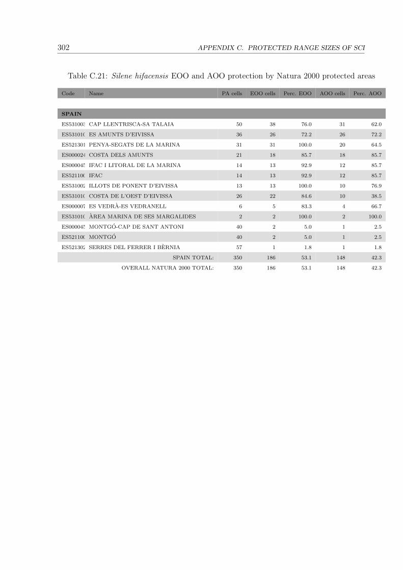
302 APPENDIX C. PROTECTED RANGE SIZES OF SCI
Table C.21: Silene hifacensis EOO and AOO protection by Natura 2000 protected areas
Code Name PA cells EOO cells Perc. EOO AOO cells Perc. AOO
SPAIN
ES5310032CAP LLENTRISCA-SA TALAIA 50 38 76.0 31 62.0
ES5310105ES AMUNTS D’EIVISSA 36 26 72.2 26 72.2
ES5213018PENYA-SEGATS DE LA MARINA 31 31 100.0 20 64.5
ES0000241COSTA DELS AMUNTS 21 18 85.7 18 85.7
ES0000459IFAC I LITORAL DE LA MARINA 14 13 92.9 12 85.7
ES5211009IFAC 14 13 92.9 12 85.7
ES5310023ILLOTS DE PONENT D’EIVISSA 13 13 100.0 10 76.9
ES5310104COSTA DE L’OEST D’EIVISSA 26 22 84.6 10 38.5
ES0000078ES VEDRA-ES VEDRANELL 6 5 83.3 4 66.7
ES5310106AREA MARINA DE SES MARGALIDES 2 2 100.0 2 100.0
ES0000454MONTGO-CAP DE SANT ANTONI 40 2 5.0 1 2.5
ES5211007MONTGO 40 2 5.0 1 2.5
ES5213020SERRES DEL FERRER I BERNIA 57 1 1.8 1 1.8
SPAIN TOTAL: 350 186 53.1 148 42.3
OVERALL NATURA 2000 TOTAL: 350 186 53.1 148 42.3

303
Table C.22: Silene hifacensis PSA protection by North African protected areas
Code Type Name PA cells PSA cells Perc. PSA
ALGERIA
72362 National Park Tigzirt 3 2 66.7
ALGERIA TOTAL: 3 2 66.7
OVERALL NORTH AFRICAN TOTAL: 3 2 66.7


Appendix D
Occurrence maps of Invasive Alien
Species
In each �gure, grey larger squares represent species occurrences at 10 km resolution while
smaller black squares represent species occurrences at 1 km resolution. All maps are in
projection Universal Transverse Mercator, Datum ED50, zone 31N (EPSG: 23031,
http://spatialreference.org/ref/epsg/23031/)
305

306 APPENDIX D. OCCURRENCE MAPS OF IAS
Figure D.1: Agave americana
Figure D.2: Ailanthus altissima

307
Figure D.3: Conyza canadensis
Figure D.4: Datura stramonium

308 APPENDIX D. OCCURRENCE MAPS OF IAS
Figure D.5: Oenothera biennis
Figure D.6: Opuntia ficus-indica

309
Figure D.7: Oxalis pes-caprae
Figure D.8: Robinia pseudoacacia
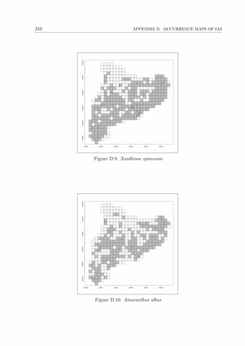
310 APPENDIX D. OCCURRENCE MAPS OF IAS
Figure D.9: Xanthium spinosum
Figure D.10: Amaranthus albus


![Catalonia[1] sp](https://static.fdocuments.in/doc/165x107/54c33b794a795980078b4591/catalonia1-sp.jpg)