Dimerization in a Tubular Reactor - Aalborg...
29
4 | CHAPTER : COMSOL MULTIPHYSICS: CHEMICAL ENGINEERING MODULE MINICOURSE Dimerization in a Tubular Reactor Tubular reactors are very common in large-scale continuous, for example in the petroleum industry. One key design and optimization parameter is the conversion, that is the amount of reactant that reacts to form the desired product. In order to achieve a high conversion, process engineers optimize the reactor design: its length, width and heating system. An accurate reactor model is a very useful tool, both at the design stage and in tuning an existing reactor. This example deals with a gas-phase dimerization process, specie A reacts to form B. First, the conversion and reaction distribution in an isothermal tubular reactor under steady-state conditions is investigated. Secondly, energy balances are included and the changes in reaction distribution and conversion are studied. Finally, a time-dependent solution is achieved, describing the process start-up. The model makes use of Maxwell-Stefan mass balance equations (which are suitable for mass transport in concentrated mixtures), a compressible formulation of the Navier-Stokes equations, and an energy balance. In the example it is demonstrated how these equations depend on each other and how they are set-up and solved fully coupled. A A+B
-
Upload
trinhhuong -
Category
Documents
-
view
233 -
download
3
Transcript of Dimerization in a Tubular Reactor - Aalborg...

4 | C H A P T E R : C O M S O L M U L T I P H Y S I C S : C H E M I C A L E N G I N E E R I N G M O D U L E M I N I C O U R S E
D ime r i z a t i o n i n a Tubu l a r R e a c t o r
Tubular reactors are very common in large-scale continuous, for example in the petroleum industry. One key design and optimization parameter is the conversion, that is the amount of reactant that reacts to form the desired product. In order to achieve a high conversion, process engineers optimize the reactor design: its length, width and heating system. An accurate reactor model is a very useful tool, both at the design stage and in tuning an existing reactor.
This example deals with a gas-phase dimerization process, specie A reacts to form B. First, the conversion and reaction distribution in an isothermal tubular reactor under steady-state conditions is investigated. Secondly, energy balances are included and the changes in reaction distribution and conversion are studied. Finally, a time-dependent solution is achieved, describing the process start-up.
The model makes use of Maxwell-Stefan mass balance equations (which are suitable for mass transport in concentrated mixtures), a compressible formulation of the Navier-Stokes equations, and an energy balance. In the example it is demonstrated how these equations depend on each other and how they are set-up and solved fully coupled.
A
A+B

D I M E R I Z A T I O N I N A TU B U L A R R E A C T O R | 5
Key Instructive Elements
This model illustrates several attractive features in the Chemical Engineering Module:
• The use of Maxwell-Stefan diffusion and convection for a concentrated solution
• The application of non-isothermal flow to model an expanding gas mixture with varying density
• The use of ready-made application mode variables to set up an expression for the mixture density
• Implementation of temperature- and composition-dependent reaction kinetics.
• The use of a mapped mesh, which is structured, to discretize a long and thin geometry, typical for tubular reactors
• The setup of thermal balances and how to couple these to both the mass balances and the velocity field
Modeling Strategy
In setting up and solving the model, you follow these steps:
1 Set up and solve a stationary isothermal model of the reactor. Here you combine the Non-Isothermal Flow application mode with the Maxwell-Stefan Convection and Diffusion application mode.
2 Set up the energy balance using the Convection and Conduction application mode. The momentum, mass, and energy balances are then solved fully coupled.
3 Solve the transient model. You run the time-dependent solver to solve the full model—including momentum, mass, and heat balances—to simulate the reactor’s startup.
Geometry
The geometry of the tubular reactor is rotationally symmetric, and it is possible to reduce the problem from 3D to a 2D axi-symmetric problem. This means that you

6 | C H A P T E R : C O M S O L M U L T I P H Y S I C S : C H E M I C A L E N G I N E E R I N G M O D U L E M I N I C O U R S E
only have to model half of the tube cross section, the shadowed part illustrated in the following figure.
Figure 1: Rotational symmetry allows you to use the axi-symmetric representation in COMSOL Multiphysics.
Modeling in COMSOL Multiphysics
1 Double-click the COMSOL Multiphysics icon on the desktop to open the Model
Navigator.
2 In the Space dimension list select Axial symmetry (2D), making sure to choose the axisymmetric option and not just plain 2D!
3 Click OK.
G E O M E T R Y
The reactor has a radius of 0.1 m and a length of 4 m.
1 Select the menu item Draw>Specify Objects>Rectangle.
2 Type 0.1 in the Width edit field, and 4 in the Height edit field.
3 Click OK.
Outlet
Inlet
r
z
Rotational symmetry

D I M E R I Z A T I O N I N A TU B U L A R R E A C T O R | 7
4 Click the Zoom Extents button on the Main toolbar.
Expanding Fluid Flow
Each mole of the reactant, A, reacts to form two moles of the product, B:
.
This leads to a volume expansion of the gas mixture as the reaction proceeds along with a corresponding decrease in the mixture density. The fluid’s change in density influences the gas velocity in the reactor, causing an acceleration as the reaction proceeds.
In order to model the flow a compressible formulation of Navier-Stokes equations is used, defined according to these equations:
Here ρ denotes the solution’s density (kg m-3), u is the velocity vector (m s-1), p gives the pressure (Pa), η represents the solution’s the viscosity (kg m-1 s-1, or Pa·s), κ is the fluid’s dilatational viscosity (kg m-1 s-1), and I denotes the identity matrix.
The density is expressed through the ideal gas law as a function of pressure, temperature, and composition:
where T denotes temperature (K), wA and wB are the mass fractions of species A and B, while MA and MB denote the molecular weight of A and B (kg mol-1), respectively.
The model uses the Non-isothermal Flow application mode, which solves the above equations, describing the momentum balances and the continuity (mass conservation) for fluids with variations in density. The application mode’s name is a bit misleading in this case because the density variations are in this case related to both temperature and composition variations. However, it uses the appropriate equations.
You will now add the application mode to the model and set up the physics.
M O D E L N A V I G A T O R
1 Select the menu item Multiphysics>Model Navigator.
A 2B→
ρt∂
∂u ρ u ∇⋅( )u+ ∇ pI– η ∇u ∇u( )T+( ) 2η 3⁄ κ–( ) ∇ u⋅( )I–+[ ]⋅=
t∂∂ρ ∇+ ρu( )⋅ 0.=
ρ pRT-------- wAMA wBMB+( )=

8 | C H A P T E R : C O M S O L M U L T I P H Y S I C S : C H E M I C A L E N G I N E E R I N G M O D U L E M I N I C O U R S E
2 On the left side of the dialog box double-click the Chemical Engineering Module
folder to expand it.
3 In the list of application modes selectChemical Engineering Module>Momentum balance>Non-Isothermal Flow.
4 Click the Add button and then click OK.
S U B D O M A I N S E T T I N G S — N O N - I S O T H E R M A L F L OW
1 From the Physics menu select Subdomain settings.
2 Select subdomain 1 in the Subdomain selection list.
3 Type rho_mix in the Density edit field.
4 In the Viscosity edit field type eta.
The dialog box should now look like this:
5 Click the Init tab.
6 In the Pressure edit field enter p_atm.
The initial pressure must be larger than zero. A zero pressure value results in zero density, which would cause the mass-balance equations to diverge in the first iteration.
7 Click OK.

D I M E R I Z A T I O N I N A TU B U L A R R E A C T O R | 9
Note: You have yet to define the expressions and values for the density, viscosity, and the initial value for pressure (rho_mix, eta, and p_atm). This is done at a later stage.
B O U N D A R Y C O N D I T I O N S — N O N - I S O T H E R M A L F L OW
The flow in the reactor is driven by a pressure drop. The pressure at the inlet, p_in, is slightly higher than at the outlet, where the pressure is set to atmospheric pressure
.
The walls are represented by no-slip boundary conditions:
.
Now set up these boundary conditions in the user interface.
1 In the Physics menu select Boundary Settings.
2 In the Boundary selection list highlight 1, then in the Boundary condition list select Axial symmetry.
3 In the Boundary selection list highlight 2. In the Boundary condition list select Normal
flow/Pressure, and in the Pressure edit field enter p_in.
4 In the Boundary selection list highlight 3. In the Boundary condition list select Normal
flow/Pressure, and in the Pressure edit field enter p_atm.
5 Click OK.
The default condition for the velocity is No slip, which applies to the remaining boundaries.
Convection and Diffusion in Multicomponent Systems
As the dimerization reaction proceeds, the mixture changes composition from pure A at the inlet to a mixture of A and B.
The total mass flux in this case is strongly influenced by the flux of each species. In addition, several molecular interactions occur; A interacts with other A molecules, A and B interact, and B interacts with other B molecules. This implies that the simple Fick’s law formulation, with one constant diffusivity for each specie, is not applicable here. In a concentrated multicomponent mixtures you must account for all possible interactions, and the flux is dependent on the fluid’s local composition. Simple Fick
p patm=
u 0=

10 | C H A P T E R : C O M S O L M U L T I P H Y S I C S : C H E M I C A L E N G I N E E R I N G M O D U L E M I N I C O U R S E
diffusivity accounts only for the interaction between solvent and solute. In the Maxwell-Stefan diffusion equations, multicomponent diffusivities describe the interaction between all components in the system.
The Maxwell-Stefan equations take the total mass balance into account. The flow is given by adding the mass fluxes of all component in the mixture. This means that a problem for n species is determined by either: n mass-balance equations, one for every species involved; or by n-1 species’ mass balances and one total mass balance, calculated as the fluid flow field.
The Maxwell-Stefan Convection and Diffusion application mode uses the second approach. It sets up n-1 species’ mass balances. A final equation is obtained from the total flow, which is set equal to the sum of all mass fluxes. The Maxwell-Stefan Convection and Diffusion application mode therefore always requires a consistent input of the velocity field, because the mass flux of the last component (species n) is determined so that the total mass flux correspond to the velocity field.
Now consider a mathematical formulation of this discussion.The mass-balance equation for each species is
with the source terms given by the reaction kinetics follow the equations
where kf denotes the forward reaction rate constant (s-1), cA represents the concentration of A (mol m-3), and ni is the mass flux vector for species i (kg m-2 s-1). Because the reaction is a pure dimerization, it is inherent that MB equals half of MA.
As mentioned earlier, it is possible to rewrite the mass-balances equations for each species by replacing one of the species’ mass balance with a total mass balance. A solution with two species follows these equations:
t∂∂ ρwA( ) ∇+ nA⋅ RA=
t∂∂ ρwB( ) ∇+ nB⋅ RB=
RA kf– cAMA=
RB 2kfcAMB=
t∂∂ ρwA( ) ∇+ nA⋅ RA=

D I M E R I Z A T I O N I N A TU B U L A R R E A C T O R | 11
.
Because the system consists only of two species, the sum of wA and wB is always unity, and the sum of the reaction terms is zero. The last equation now becomes
,
which is the total mass-balance equation.
Reaction rate
The dimerization reaction studied here is assumed to be irreversible.
The reaction rate is described by an Arrhenius law according to:
where A0, the pre-exponential factor, is set to 41.3 (s-1), Ea, the activation energy, is set to 30 (kJ mol-1), R is the gas constant, 8.314 (J mol-1 K-1), and T the temperature (K).
The rate of production of species B is thus dependent on both composition and temperature. However, in this first model the gas is assumed to be isothermal, making the rate vary only with composition.
M O D E L N A V I G A T O R
1 Select the menu item Multiphysics>Model Navigator.
2 Select the application mode Chemical Engineering Module>Mass balance>Maxwell-Stefan Diffusion and Convection.
3 Find the Dependent variables edit field, and type wA and wB in it.
4 Click Add.
t∂∂ ρ wA wB+( )( ) ∇+ nA n+ B( )⋅ RA RB+=
t∂∂ρ ∇+ nA n+ B( )⋅ 0=
A 2B→
kf A0Ea–
RT----------
⎝ ⎠⎛ ⎞exp=

12 | C H A P T E R : C O M S O L M U L T I P H Y S I C S : C H E M I C A L E N G I N E E R I N G M O D U L E M I N I C O U R S E
The Model Navigator should now look like this:
5 Click OK.
S U B D O M A I N S E T T I N G S — M A X W E L L - S T E F A N
1 From the Physics menu select Subdomain Settings.
2 In the Subdomain selection list select subdomain 1.
3 In the Density edit field enter rho_mix; in the Pressure edit field enter p; and in the Temperature edit field enter T.
4 In the r-velocity enter u, and in the z-velocity edit field enter v.
Note: p, u, and v are the notations for the dependent variables in the Non-Isothermal Flow application mode. A relevant question is why the software does not automatically enter them in the respective edit fields. The reason is that in some models you might want to use several velocity fields (2-phase flow) or define an analytical expression for p, u, and v.
Continue now with the Maxwell-Stefan diffusivity matrix:
5 Click the Edit button for the Maxwell-Stefan diffusivity matrix.
6 Enter DA in the only available edit field (position (1, 2)).

D I M E R I Z A T I O N I N A TU B U L A R R E A C T O R | 13
7 Click OK in the Maxwell-Stefan diffusivity matrix dialog box.
Before you close the Subdomain settings dialog box, you must specify the properties for each species:
8 Click the wA tab. In the Molecular weight edit field enter MA, and in the Reaction rate
edit field enter -Ra.
9 Click the wB tab. In the Molecular weight edit field type MB.
10 Click OK.
B O U N D A R Y C O N D I T I O N S — M A X W E L L - S T E F A N
At the inlet, the mass fraction of A is set to unity,
,
while the outlet boundary condition is a convective flux condition
with n denoting the normal vector to the boundary.
The convective flux condition implies that diffusive flux for the species is zero perpendicular to the boundary. This is a common assumption when modeling the outlet in tubular reactors.
At all other boundaries you can apply no-flux conditions, denoted in COMSOL Multiphysics as insulation/symmetry:
1 From the Physics menu select Boundary Settings.
2 In the Boundary selection list highlight 1, then in the Boundary condition list select Axial symmetry.
3 In the Boundary selection list highlight 2. In the Boundary Condition list select Mass
fraction, then in the Mass fraction edit field enter wA_in.
4 In the Boundary selection list highlight 3, then in the Boundary condition list select Convective flux.
5 Click OK.
The remaining boundaries use the default condition Insulation/Symmetry.
wA wA0=
n nA⋅ n wAρu( )⋅=
n n⋅ A 0.=

14 | C H A P T E R : C O M S O L M U L T I P H Y S I C S : C H E M I C A L E N G I N E E R I N G M O D U L E M I N I C O U R S E
C O N S T A N T S
You are now ready to define the constants used in the model. They describe material data such as viscosity as well as problem-dependent properties such as inlet conditions. The Constant list can be considered a temporary database in the model where you make changes only in one place but whose entries influence all the edit fields that include such constants.
1 Select the menu item Options>Constants and type in the following data in the Name,Expression, and Description edit fields:
Note: COMSOL Multiphysics supports automatic unit analysis, and conversion to the base unit system of the model. You can define the unit of a constant by using the syntax above. You can switch on automatic warning for unit inconsistencies in your formulas by entering the Options>Preferences>Modeling and check Highlight
Unexpected Units.
The Constants dialog box should now look like this:
NAME EXPRESSION DESCRIPTION
eta 3e-5[Pa*s] Viscosity
p_atm 1.013e5[Pa] Pressure
T 473[K] Temperature
DA 1e-5[m^2/s] Diffusivity
MA 16e-3[kg/mol] Mole mass of A
MB 8e-3[kg/mol] Mole mass of B
Rg 8.314[J/mol/K] Gas constant
p_in p_atm+8e-3[Pa] Pressure at inlet
wA_in 1[1] Mass fraction of A at inlet

D I M E R I Z A T I O N I N A TU B U L A R R E A C T O R | 15
2 Click OK.
S C A L A R E X P R E S S I O N S
In this model you define most of the multiphysics couplings in the Scalar Expressions
dialog box:
• Specify the density as an expression of pressure, concentration, and temperature.
• Specify the rate coefficient as being temperature dependent.
• The rate expression relates the species concentration (which is a function of mole fraction, pressure and temperature) to the reaction rate.
• In addition, you define the inlet velocity profile, which here is a function of the radial position.
To define the scalar expression list, follow these steps:
1 From the Options menu select Expressions>Scalar Expressions and add the following Name, Expression, and Description settings:
The Scalar Expressions dialog box should now look like this:
2 Click OK.
You have now defined all the constants and variables in the expressions given earlier except for the mole fractions x_wA_chms and x_wB_chms. These are internal variables.
NAME EXPRESSION DESCRIPTION
cwA x_wA_chms*p/Rg/T Concentration of A
cwB x_wB_chms*p/Rg/T Concentration of B
rho_mix MA*cwA+MB*cwB Density of the mixture
kf 41.3*exp(-30e3/Rg/T) Rate function
Ra kf*cwA*MA Reaction rate

16 | C H A P T E R : C O M S O L M U L T I P H Y S I C S : C H E M I C A L E N G I N E E R I N G M O D U L E M I N I C O U R S E
You can verify that you have used the correct notation for the mole fractions with the following procedure:
1 From the Physics menu select Equation systems>Subdomain Settings.
2 In the Subdomain selection list highlight 1.
3 Click the Variables tab.
4 Scroll down until you find the mole fractions as in the following figure:
5 Now that you have confirmed that the correct notations for the mole fractions are being used, click Cancel to continue.
M E S H G E N E R A T I O N
In this example, a mapped (structured) mesh is a good choice due to the reactor’s regular shape. A mapped mesh gives full control of the elements’ width/length relationship. The use of a structured mesh is especially suitable when the requirements for the mesh density are greater in one direction (radial) than the other (axial). In this example a denser mesh is required in the inlet region to resolve gradients at the inlet. This is achieved by specifying the edge element distribution, as you see below.
1 From the Mesh menu select Map mesh.
2 Click the Boundary tab.
3 Go to the Boundary selection list and highlight 1 and 4 (press Ctrl while selecting to highlight both), then click to select the Constrained edge element distribution
checkbox.
4 Click to select Edge vertex distribution and type 0 1/400 1/200 1/100:1/50:1 in the corresponding edit field.

D I M E R I Z A T I O N I N A TU B U L A R R E A C T O R | 17
5 In the Boundary selection list highlight 2, then select the Constrained edge element
distribution checkbox. In the Number of edge elements edit field enter 5.
6 Click Remesh, then click OK.
COMSOL Multiphysics should create a mesh consisting of 260 elements. You can see the reported number of generated elements in the Status bar at the bottom of the main window.
C O M P U T I N G T H E S O L U T I O N
1 From the Solve menu select Solver Parameters.
2 Click the Advanced tab.
3 In the Type of scaling list select Initial value based.
The option of initial-value based scaling is a better alternative than the default of automatic scaling due to the difference in magnitude of the components of the solution (u, v, p, and wA). When you define an estimate of the magnitude of the different components before running the solver, it obtains a more appropriate measure of the residual and indirectly of the accuracy of the numerical solution.
For this particular model it is the radial velocity, which is close to zero, that could cause problems unless the scaling is specified.
4 Click OK.
5 Click the Solve button (=) on the Main toolbar.
P O S T P R O C E S S I N G A N D V I S U A L I Z A T I O N
The default plot shows the velocity field in the reactor. By default the software plots it using equal geometrical scales on the r- and z-axes. However, in this case it is more convenient to use non-equal axis settings.
1 To allow non-equal axis settings, double-click the Equal field in the Status bar at the bottom of the user interface.

18 | C H A P T E R : C O M S O L M U L T I P H Y S I C S : C H E M I C A L E N G I N E E R I N G M O D U L E M I N I C O U R S E
2 Click the Zoom Extents button on the Main toolbar. You should get this figure:
The fluid velocity increases along the axis of the reactor. This is caused by the expansion of the mixture due to the reaction. However, from this image it is difficult to evaluate exactly how much it varies and what the velocity profile looks like. You can use radial cross sections along the reactor to visualize the velocity profiles better.
3 From the Postprocessing menu select Cross-Section Plot Parameters.
4 Click the Line/Extrusion tab.
5 In the Predefined quantity list select Velocity field (chns).
6 Go to the r0 edit field and enter 0, then in the r1 edit field type 0.1.
7 Type 0 in both the z0 and z1 edit fields.
8 Select the Multiple parallel lines checkbox.
9 Click the Vector with distances button. In the Vector with distances edit field enter linspace(0.5,4,11). This creates 11 cross sections parallel to the first cross section with offsets of 0 to 4 meter (from inlet to outlet).
10 Click the Line settings button. Select the Legend checkbox, then click OK. This generates a legend next to the graph.
11 Click the General tab.

D I M E R I Z A T I O N I N A TU B U L A R R E A C T O R | 19
12 Click the Title/Axis button. Click the option button and in the First axis label edit field type Position, r [m]. Click OK.
13 Click OK in the Cross-Section Plot Parameters dialog box to create the following plot:
Now it is easier to see the velocity profiles along the reactor, and how the velocity increases.
To evaluate the reactor’s performance, you can plot the mole fraction of A at the same radial cross sections just used.
1 From the Postprocessing menu select Cross-Section Plot Parameters.
2 Click the Line/Extrusion tab.
3 Find the y-axis data area and in the Expression edit field enter x_wA_chms.
4 On the General page click the Title/Axis button.

20 | C H A P T E R : C O M S O L M U L T I P H Y S I C S : C H E M I C A L E N G I N E E R I N G M O D U L E M I N I C O U R S E
5 Specify Title and Axis labels according to the following figure, then click OK.
6 Click OK in the Cross-Section Plot Parameters dialog box to create the following plot:
Under the present operating conditions, the mole fraction of A decreases from unity at the inlet to approximately 0.3 at the outlet. This means that the conversion is approximately 70%. The reaction rate is proportional to the partial pressure of A, and because the relative pressure drop over the reactor is very small, the reaction rate distribution is almost identical to the plot just shown.
To get an even better measurement of the reactor performance you can compute the average value of the conversion at the outlet. In this case, you are interested in the cup-mixing average of the conversion at the outlet, taking the flow rate profile into account. The cup-mixing average represents the value you would get if you sampled a volume for a certain time in a cup, mixed it, and then measured the value. It is defined according to

D I M E R I Z A T I O N I N A TU B U L A R R E A C T O R | 21
.
To evaluate γB at the outlet, you need to evaluate the two integrals in the formula above. This is done with the boundary integration-coupling variables.
1 Select the menu item Options>Integration Coupling Variables>Boundary Variables.
2 In the Boundary selection list highlight 3 (the outlet).
3 Add the following Name and Expression settings:
Note: You must include 2*pi*r in the integral variables because you are computing the surface integral at the reactor’s outlet.
4 Use the default values for Integration order (4) and Global destination.
The Boundary Integration Variables dialog box should now look like this:
5 Click OK.
6 From the Solve menu select Update Model. By updating the model you make the new variables available without having to solve the entire system again.
7 From the Postprocessing menu select Data Display>Global.
NAME EXPRESSION
cup_mix rho_mix*v*(1-x_wA_chms)*2*pi*r/mass_mix
mass_mix rho_mix*v*2*pi*r
γB
1 XA–( )ρu n⋅ sd∫ρu n⋅ sd∫
------------------------------------------------=

22 | C H A P T E R : C O M S O L M U L T I P H Y S I C S : C H E M I C A L E N G I N E E R I N G M O D U L E M I N I C O U R S E
8 Go to the Expression to evaluate edit field, enter cup_mix, then click OK.
The value of the cup_mix expression is reported in the Log field at the bottom of the graphical user interface. In this case the software reports approximately a 77% cup mixing rate.
Non-Isothermal Model
Now it is time to expand the model by including an energy-balance equation modeling the temperature. In the previous model, the temperature was constant and set to 473 K. However, now assume that the gas enters the reactor at room temperature, 293 K, and that the reactor walls are heated to 473 K to accomplish heating of the gas and reaction. This means that the gas is heated by the walls as the gas flows along the reactor. In addition, the heat of reaction is also included, acting as a source term. For the current dimerization reaction the heat of reaction is -20 kJ mol-1. This means that the fluid mixture is heated as the reaction proceeds.
The influence of the temperature variation on the reaction rate is significant. The rate follows an Arrhenius law, it increases exponentially with temperature. Thus, the reaction rate increases as the fluid flows through the reactor and is heated by the walls and by the heat of reaction.
The energy-balance equation is
where k is the thermal conductivity (W m-1 K-1), Cp is the specific heat capacity (J kg-1
K-1), and Q is the heat-source term (W m-3).
The heat source term, Q, is given by the heat of reaction, ∆H (-20 000), and reaction rate, R:
The material properties are specified to be those of the mixture. In this example assume that the heat capacity, Cp, and conductivity, k, are similar to those of propane, which is present in the Material Library.
The boundary conditions for the energy balance are similar to those of the mass balances. At the inlet, the gas temperature is specified, in this case to 293 K.
Symmetry is applied at the symmetry boundary, meaning zero temperature gradient.
ρCp t∂∂T ∇ k T∇–( )⋅+ Q ρCpu T∇⋅–=
Q ∆– HRA=

D I M E R I Z A T I O N I N A TU B U L A R R E A C T O R | 23
.
At the outlet, convective flux is applied,
.
Model the reactors heated walls by applying a heat flux condition on the wall, using a heat transfer coefficient, h, (50 W m-2 K-1) for the heating fluid, and the heating fluids temperature, Tf, which is 473 K. The condition is:
M O D E L N A V I G A T O R
1 From the Multiphysics menu select Model Navigator.
2 Double-click the Energy Balance folder to expand it.
3 In the list of application modes select Chemical Engineering Module>Energy Balance>Convection and Conduction.
4 Click Add, then click OK.
S U B D O M A I N S E T T I N G S — C O N V E C T I O N A N D C O N D U C T I O N
1 From the Physics menu select Subdomain Settings.
2 In the Subdomain selection list highlight 1.
3 In the Thermal conductivity edit field type k_mix; in the Density edit field enter rho_mix, and in the Heat capacity edit field enter Cp_mix.
4 Type 80e3*Ra in the Heat source edit field.
5 Go to the r-velocity edit field and enter u, then in the z-velocity edit field enter v.
6 Click the Init tab.
7 In the Temperature edit field enter T_atm.
8 Click OK.
B O U N D A R Y C O N D I T I O N S — C O N V E C T I O N A N D C O N D U C T I O N
1 From the Physics menu select Boundary Settings.
2 In the Boundary selection list highlight 1, then in the Boundary condition list select Axial symmetry.
3 In the Boundary selection list highlight 2. In the Boundary condition list select Temperature, and in the Temperature edit field enter T_atm.
n T∇⋅ 0=
n T∇⋅ 0=
n k T∇( )⋅ h Tf T )–( )=

24 | C H A P T E R : C O M S O L M U L T I P H Y S I C S : C H E M I C A L E N G I N E E R I N G M O D U L E M I N I C O U R S E
4 In the Boundary selection list highlight 3, then in the Boundary condition list select Convective flux.
5 In the Boundary selection list highlight 4. In the Boundary condition list select Heat
flux, and type 50*(Tf-T) in the Heat flux edit field.
6 Click OK.
C O N S T A N T S A N D E X P R E S S I O N S
At this point T is a dependent variable in the energy balance, so you must rename the constant T that you defined in the previous model.
1 From the Options menu select Constants.
2 In the Name field rename the variable T (on the third row) to T_atm and change the value to 293.
3 Add the following settings in the Constants dialog box:
4 The Constants dialog box should now look like this:
5 Click OK.
You must also define the thermal conductivity, which is a function of temperature.
1 From the Options menu select Expressions>Scalar Expressions and add the following Name, Expression, and Description settings:
NAME EXPRESSION DESCRIPTION
Tf 473[K] Temperature of heating fluid
Cp_mix 1700[J/kg/K] Heat capacity of mixture
NAME EXPRESSION DESCRIPTION
k_mix 10^(0.7123*log10(abs(T))-3.4152) Thermal conductivity

D I M E R I Z A T I O N I N A TU B U L A R R E A C T O R | 25
2 The Scalar Expressions dialog box should now look like this:
3 Click OK.
C O M P U T I N G T H E S O L U T I O N
1 From the Solve menu select Get Initial Value.
2 Click the Solve button (=) on the Main toolbar.
P O S T P R O C E S S I N G
Start by plotting the temperature field.
1 From the Postprocessing menu select Plot Parameters.
2 Click the Surface tab.
3 In the Predefined quantities menu select Temperature(chcc).
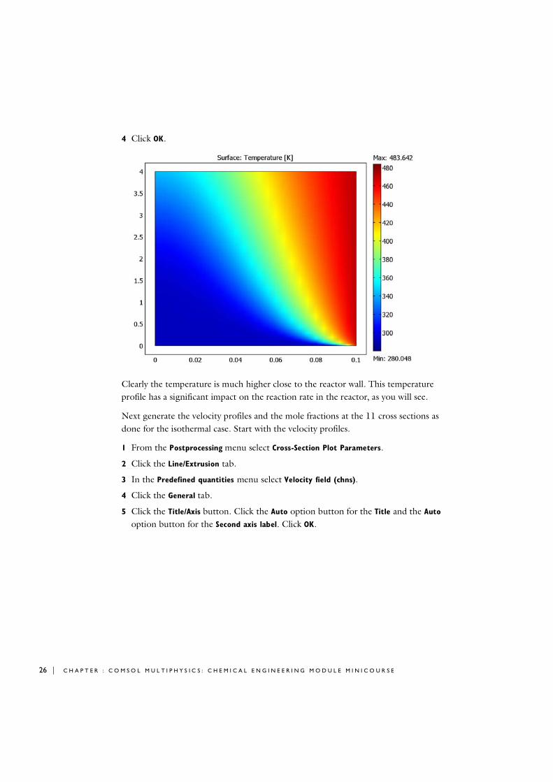
26 | C H A P T E R : C O M S O L M U L T I P H Y S I C S : C H E M I C A L E N G I N E E R I N G M O D U L E M I N I C O U R S E
4 Click OK.
Clearly the temperature is much higher close to the reactor wall. This temperature profile has a significant impact on the reaction rate in the reactor, as you will see.
Next generate the velocity profiles and the mole fractions at the 11 cross sections as done for the isothermal case. Start with the velocity profiles.
1 From the Postprocessing menu select Cross-Section Plot Parameters.
2 Click the Line/Extrusion tab.
3 In the Predefined quantities menu select Velocity field (chns).
4 Click the General tab.
5 Click the Title/Axis button. Click the Auto option button for the Title and the Auto
option button for the Second axis label. Click OK.

D I M E R I Z A T I O N I N A TU B U L A R R E A C T O R | 27
6 Click OK to generate the following figure:
As you can see, the maximum velocity along the axis of the reactor increases by only approximately 40% (from 0.10 to 0.14 m/s) for the non-isothermal case, compared to 66% for the isothermal case. This is caused by the lower reaction rate.
You can generate the mole fraction of A in a similar manner as before:
1 From the Postprocessing menu select Cross-Section Plot Parameters.
2 Click the Line/Extrusion tab.
3 Locate the y-axis data area and in the Expression edit field enter x_wA_chms.
4 Click the General tab.
5 Click the Title/Axis button. Click the option button for the Title edit field and enterMole fraction of A; click the option button for the Second axis label edit field and enter Mole fraction. Click OK.

28 | C H A P T E R : C O M S O L M U L T I P H Y S I C S : C H E M I C A L E N G I N E E R I N G M O D U L E M I N I C O U R S E
6 Click OK to generate the following figure:
The conversion of A has decreased significantly in the non-isothermal case, especially in the center of the reactor where the temperature is low. As you can see from the figure, most of reactions take place along the wall. One way of increasing the conversion would be to increase the wall temperature.
Before moving on, study the cup mixing of A.
1 From the Postprocessing menu select Data Display>Global.
2 In the Expression to evaluate edit field enter cup_mix, then click OK.
The value of the cup_mix expression is reported in the bottom of the main window. This time you get only approximately a 33% cup mixing rate.
Transient Analysis of a Startup Sequence
Now you will perform a transient startup study of the non-isothermal reactor. It is interesting to see the time necessary to reach steady-state, and also the behavior of the reactor during start-up from atmospheric conditions.
It is easy to switch between a steady-state and a transient analysis in COMSOL Multiphysics. This is done by changing to time-dependent solver. However, first you

D I M E R I Z A T I O N I N A TU B U L A R R E A C T O R | 29
must specify the initial value for wA in the Maxwell-Stefan’s equations. Assume a weight fraction of a that is 99.99%.
Note: The Maxwell Stefan binary formulation is only valid for two components. Therefore you cannot specify an initial 100% concentration of A, since that corresponds to a single component system.
S U B D O M A I N S E T T I N G S
1 From the Multiphysics menu select the Maxwell-Stefan Diffusion and Convection (chms)
application mode.
2 From the Physics menu select Subdomain Settings.
3 In the Subdomain selection highlight 1.
4 On the Init page find the Mass fraction, wA edit field and enter 0.9999.
5 Click OK.
C O M P U T I N G T H E S O L U T I O N
You are now ready to solve the time-dependent problem:
1 From the Solve menu select Solver Parameters.
2 Click the General tab.
3 In the Solver list select Time dependent.
4 Go to the Time stepping area, and in the Times edit field enter 0:2:240.
5 Change the tolerance for the solver. In the Absolute tolerance edit fields enter 0.1.This improves solution speed by making the solver neglect errors in all variables that are smaller than 0.1 in absolute scale. The accuracy will then be controlled in a relative scale with less than 1% error (as specified by Relative tolerance 0.01)
6 Click the Time Stepping tab.
7 Change the Time steps taken by solver to Intermediate.
8 Click OK.
9 Click the Solve button (=) on the Main toolbar. The solution process takes approximately 1 minutes (for a 1.6 GHz Laptop). You can notice that most of the time is spent on solving for the first second. That is when most of the dynamics in the system appears.

30 | C H A P T E R : C O M S O L M U L T I P H Y S I C S : C H E M I C A L E N G I N E E R I N G M O D U L E M I N I C O U R S E
P O S T P R O C E S S I N G
Create an animation of the temperature to illustrate how the temperature field evolves over time. This gives a first answer to the main question: After how long time is the reactor stationary?
1 From the Postprocessing menu select Plot Parameters.
2 Click the Surface tab.
3 In the Predefined quantities list select Temperature(chcc).
4 Click the Animate tab.
5 Select Interpolated times from the Select via list in the Solutions to use area.
6 Type 0:10:240 in the Times edit field. This will generate a movie with a constant time step size of 10 seconds.
7 Click the Start Animation button. COMSOL Multiphysics generates each movie image. This process takes a few seconds. Then the movie can be played by clicking the Play button in the COMSOL Movie Player window.
The movie shows that the temperature field evolves during the first 120 seconds and then behaves rather stationary. However, our main interest is the conversion. Let’s plot the average outlet conversion as a function of time.
8 Close the Movie Player window.
9 Click OK to close the Plot Parameters dialog.
10 From the Postprocessing menu select Global Variables Plot.
11 In the Expression edit field enter cup_mix.
12 Click the Add Entered Expression button (>) to the right of the Expression edit field such that the variable cup_mix shows up in the Quantities to plot list.
13 In the Solutions to use list verify that all the time steps are selected.
14 Click the Title/Axis button.
15 Select the option button for the Title edit field and enter Cup mixing fraction of A; then select the option button for the Second axis label edit field and enter Cupmixing.
16 Click OK to close the Title/Axis Settings dialog box.

D I M E R I Z A T I O N I N A TU B U L A R R E A C T O R | 31
17 Click OK in the Global Variables Plot dialog box to create this plot:

32 | C H A P T E R : C O M S O L M U L T I P H Y S I C S : C H E M I C A L E N G I N E E R I N G M O D U L E M I N I C O U R S E
As you can see, after approximately 150 seconds the process seem to have reached steady-state.