Dimensional Analysis, Leverage Neutrality,

and Market Microstructure Invariance

Albert S. Kyle and Anna A. Obizhaeva*

First draft: September 17, 2015

This draft: January 13, 2019

Abstract

This paper combines dimensional analysis, leverage neutrality, and a principle of mar-

ket microstructure invariance to derive scaling laws expressing transaction costs functions,

bid-ask spreads, bet sizes, number of bets, and other financial variables in terms of dollar

trading volume and volatility. The scaling laws are illustrated using data on bid-ask spreads

and number of trades for Russian and U.S. stocks. These scaling laws provide practical met-

rics for risk managers and traders; scientific benchmarks for evaluating controversial issues

related to high frequency trading, market crashes, and liquidity measurement; and guide-

lines for designing policies in the aftermath of financial crisis.

JEL Codes: G10, G12, G14, G20.

Keywords: market microstructure, liquidity, bid-ask spread, trade size, market depth, dimen-

sional analysis, leverage, invariance, econophysics.

*Kyle: University of Maryland, College Park, MD 20742, USA, akyle@rhsmith.umd.edu. Obizhaeva: New Eco-

nomic School, Moscow, Skolkovo, 143026, Russia, aobizhaeva@nes.ru. The authors thank Bo Hu and Thomas

James for helpful comments as well as Sylvain Delalay for his assistance.

This paper combines dimensional analysis, leverage neutrality, and a market microstructure

invariance hypothesis to derive scaling laws for the specification of transaction cost functions,

the width of bid-ask spreads, the size distribution of bets or trades, the speed of bet or trade

execution, the size of margin requirements and haircuts, optimal minimum increments of price

fluctuations (tick size), and optimal increments of traded quantities (minimum lot size). The

basic liquidity measure is proportional to the cube root of the ratio of dollar volume to return

variance. Bid-ask spreads, which measure the difference between the highest price at which a

trader is willing to buy (“bid”) and the lowest price at which a trader is willing to sell (“offer”), are

predicted to be inversely proportional to this liquidity measure. The rate at which trades arrive

is predicted to be proportional to the product of the liquidity measure squared and volatility

squared. The scaling is illustrated by showing that both bid-ask spreads and the number of

trades indeed scale as predicted in both the Russian and U.S. stock markets.

In financial markets, institutional investors trade by implementing speculative “bets” which

move prices. A bet is a decision to buy or sell a quantity of institutional size. In the stock mar-

ket, traders execute bets by dividing them into separate orders, shredding the orders into small

pieces, and executing numerous smaller quantities over time. Across different stocks, the time

frame of execution may be minutes, hours, days, or weeks. The fields of market microstructure

and econophysics use different but complementary approaches for studying how prices result

from trading securities. As emphasized by Gabaix et al. (2003), large trades incur trading costs

by moving prices. Foucault, Pagano and Roell (2013) and Bouchaud, Farmer and Lillo (2009)

summarize various findings from the perspectives of market microstructure and econophysics,

respectively.

Dimensional analysis simplifies scientific inference by imposing restrictions on unknown

and potentially complicated relationships among different variables. In physics, researchers

obtain powerful results by using dimensional analysis to reduce the dimensionality of prob-

lems, as reviewed in Barenblatt (1996). For example, Kolmogorov (1941) proposed a simple

dimensional analysis argument to derive his “5/3–law” for the energy distribution in a turbu-

lent fluid. Dimensional analysis can be also used to infer the size and number of molecules in

a mole of gas or the size of the explosive energy in an atomic blast from measurable large-scale

physical quantities. In this paper, we apply dimensional analysis to an economic problem using

an approach which mimics the way physicists apply dimensional analysis to physics problems.

This paper derives new results by using dimensional analysis to relate market liquidity to dollar

volume and returns volatility. Our analysis takes place in three steps which mimic the use of

dimensional analysis in physics.

First, in physics, dimensional analysis begins with fundamental units of mass, distance, and

time. In finance, dimensional analysis begins with fundamental units of asset quantity, value,

1

and time. The problem is simplified by constructing dimensionless ratios of dimensional quan-

tities measuring asset prices, trading volumes, returns volatilities, and costs of making bets.

Second, physics researchers augment dimensional analysis with conservation laws based

on principles of physics, such as the law of conservation of energy. In finance, proceeding fur-

ther requires introducing conservation laws based on principles of finance. Since no-arbitrage

principles—like Black and Scholes (1973) use to derive their option pricing model—are so fun-

damental to finance, the financial conservation laws naturally take the form of no-arbitrage

restrictions. Here we use the less restrictive, more simplistic no-arbitrage principle of leverage

neutrality. Since cash is a risk-free asset, transfers of cash between traders occur at zero cost;

riskless, cash-equivalent assets are infinitely liquid. If a risky asset is combined with a positive

or negative amount of a cash-equivalent asset and this bundle then is traded as a single pack-

age, the economics behind trading this package does not depend on how much cash is included

into it. This does not create arbitrage opportunities.

Leverage neutrality captures the intuition of Modigliani and Miller (1958) that a firm’s mix

of equity and riskfree debt securities does not affect the value of a firm. Leverage neutrality

implies that changes in a security’s volatility, resulting from the amount of riskfree debt used

to finance a firm, do not affect the economic outcomes associated with execution of bets that

transfer risks embedded in the firm’s securities. Leverage neutrality is also related to the idea

that changes in margin requirements and repo haircuts do not affect the costs of transferring

risks.

Third, physics researchers often take as given dimensional constants which do not vary dur-

ing the analysis, such as the acceleration of gravity at sea level on the planet earth. Here we

make the invariance assumption that the expected dollar cost of executing a bet is constant

across assets and time. We refer to this assumption as market microstructure invariance. This

leads to specific testable empirical scaling hypotheses with exponents of 1/3 or 2/3. In market

microstructure, dimensional analysis leads to new insights which are neither obvious nor well-

known. For example, predictions about microscopic financial quantities like the size of bets

and the width of bid-ask spreads can be made based on observing macroscopic quantities like

aggregate dollar volume and returns volatility.

As an alternative to dimensional analysis, analogous results can be derived in two different

ways: (1) directly from empirical invariance hypotheses or (2) as properties of an equilibrium

model. While all three approaches are consistent with one another, each of them generates new

insights about invariance and has some advantages over the other two.

First, Kyle and Obizhaeva (2016c) derive and test scaling laws using two empirical invariance

conjectures based on analyzing trading in business time. They hypothesize that (1) the dollar

risk transferred by bets and (2) the dollar costs of executing bets, transferring economically

2

equivalent risks, are the same across securities and time. This approach implicitly incorporates

leverage neutrality. Dimensional analysis is more general because it can easily be generalized

to include other explanatory variables and to generate new quantitative predictions about vari-

ables of interest.

Second, Kyle and Obizhaeva (2016b) take the alternative approach of deriving scaling laws

as endogenous implications of a dynamic equilibrium model with a specific structure, which

assumes that the effort required to generate one discrete bet does not vary across securities and

time. This assumption is closely related to this paper’s assumption of an invariant expected

execution cost for each bet. Risk-neutral informed traders make bets whose frequency and

size depend on expected trading profits constrained by endogenous market depth, not exoge-

nous risk aversion. For analytical tractability, the model makes the restrictive assumption that

traders make only one bet whose size is observed by liquidity providers taking the other side of

the trade. Since dimensional analysis eschews making connections to specific micro-founded

economic models, it suggests that our predictions may hold under more general assumptions.

When market observations deviate from what is expected, predictions derived from dimen-

sional analysis provide a benchmark from which to interpret the economic meaning of the de-

viations. For example, a physicist might use a pendulum swinging in a vacuum as a benchmark

from which to model the effects of the earth’s atmosphere on a swinging pendulum. In market

microstructure, deviations from benchmark predictions might result from omitting economi-

cally important variables or market frictions from the simplest specifications based on dimen-

sional analysis. Dimensional analysis can therefore help evaluate the effects of omitted vari-

ables, such as time horizon of bet execution, or omitted frictions, such as minimum tick size

and minimum lots size. It leads to a natural scientific process both for discovering new rela-

tionships among financial variables and for extending them in an internally consistent manner

to include other explanatory variables. Using a generalized dimensional analysis algorithm,

we augment a basic transaction cost formula by adding differences in execution horizons and

variations in market frictions related to minimum tick size and minimum lot size.

Dimensional analysis per se does not guarantee success; rather, it helps to narrow alterna-

tives to more promising paths for research. Leverage neutrality and microstructure invariance

suggest additional restrictions based on the economics behind underlying processes. The ulti-

mate check for validity of any theory is whether its predictions can be backed by empirical ev-

idence. Our empirical evidence suggests that dimensional analysis does indeed establish good

empirical benchmarks for analyzing trade size and bid-ask spreads.

Our predictions can be stated as power laws, which define log-linear relationships between

finance quantities with specific exponents of 1/3 and 2/3; these relationships resemble famil-

iar laws of physics. A related but different literature in finance and economics studies power

3

laws which show up mostly in the tails of frequency distributions of financial variables such

as trade size or returns. This literature is reviewed in Sornette (2004), Newman (2005), Gabaix

et al. (2006), and Gabaix (2009). Gabaix et al. (2006) find an observed power law for trading

volume and trade size of 3/2 and an observed power law of 3 for returns; they show that this is

consistent with a square root model of price impact. The square root model of price impact is

also consistent with the most parsimonious application of dimensional analysis. An interesting

issue for future research is to understand whether the specific exponents documented in this

literature on power laws are consistent with the exponents of 1/3 and 2/3 that we derive here.

This paper is organized as follows. Section 1 discusses application of dimensional analysis

to transaction cost modeling. Section 2 introduces leverage neutrality. Section 3 discusses the

economic interpretation of some variables. Section 4 describes market microstructure invari-

ance. Section 5 presents empirical evidence using data from the Russian and U.S. stock markets.

Section 6 outlines a general algorithm for handling misspecified models with too many or too

few variables. Section 7 extends the analysis to other variables and concludes.

1 Dimensional Analysis.

In financial markets, traders exchange risky assets. Asset prices reveal information that influ-

ences resource allocation. Speculative traders develop trading ideas based on private infor-

mation they acquire conducting securities research. Hedgers buy or sell risky assets to better

allocate risk. Bets are sequences of speculative or hedging transactions to trade in the same

direction based on the same—approximately independently distributed—information or mo-

tives.

Exchanging risks via trading securities is costly because execution of bets moves market

prices. Buy bets push prices up and sell bets push prices down relative to pre-trade price bench-

marks. This market impact occurs as a result of adverse selection. Since traders on the opposite

sides of bets believe that bets may contain private information, they require a price conces-

sion as compensation. Transaction cost models quantify trading costs. Good transaction cost

models are of great interest to traders.

We next use dimensional analysis to derive an internally consistent model of transaction

costs. We follow the step-by-step procedure outlined by Barenblatt (1996) for non-finance ap-

plications. Dimensional analysis leads to scaling laws proportional to products of powers of

explanatory variables with different exponents. Dimensional analysis pays careful attention to

maintaining consistency of dimensions and units of measurement. In physics, the base dimen-

sions are considered to be length, measured in meters; mass, measured in kilograms; and time,

measured in seconds.

4

When finance researchers describe trading in financial markets, the base dimensions are

value, measured in units of currency; asset quantity, measured in units of shares or contracts;

and time, measured in units of years, months, days, hours, minutes, seconds, milliseconds, or

even microseconds. In this paper, we measure value in U.S. dollars (USD) or Russian rubles

(RUB), asset quantity in shares, and time in days.

Let P j t denote the stock price, V j t its share volume, and σ2j t its return variance, where the

subscript j t refers to stock j at time t . Let Q j t denote the number of shares traded in a bet,

with Q j t > 0 representing buying and Q j t < 0 representing selling. Let G j t denote the expected

price impact cost of executing the bet of Q j t shares as a fraction of the unsigned value traded

∣P j t ⋅Q j t ∣, with G j t ≥ 0.

We next show how to apply dimensional analysis for transaction cost modeling to make

predictions about G j t . Applying dimensional analysis correctly requires selecting the right set

of variables to construct a model which explains the variable of interest.

Assumption 1 (Dimensional Analysis). The market impact cost G j t of executing a bet of Q j t

shares is a function of only five variables: the number of shares Q j t , the stock price P j t , share

volume V j t , return variance σ2j t , and expected dollar “bet cost” C :

G j t ∶= g(Q j t ,P j t ,V j t ,σ2j t ,C). (1)

Writing g instead of g j t reflects the important assumption that the price impact cost is a

function only of its parameters and not other characteristics of asset j at time t . The variable C

is key in our invariance framework. It is defined as the unconditional expected dollar costs of

executing a bet,

C ∶=E{G j t ⋅ ∣P j t ⋅Q j t ∣}. (2)

The value of C may be difficult to observe empirically. The hypothesis of market microstructure

invariance, discussed below, implies that C may be written without subscripts j t .1 For now,

we assume that equation (1) is a correctly specified model that does not omit important ex-

planatory variables. Later, we illustrate conceptually how to improve a misspecified model by

including omitted variables such as tick size or minimum lot size.

Dimensional analysis requires paying careful attention to consistency of the units in which

these quantities are measured. Let brackets [X ] define an operator which gives the dimensions

of a variable X . Using this notation, the function arguments Q j t , P j t , V j t , σ2j t

, and C are mea-

1In Kyle and Obizhaeva (2016c), the average dollar bet cost C is denoted C̄B , and the percentage cost G j t of

executing a bet of size Q is denoted C j t(Q).

5

sured using units of currency, shares, and time as follows:

[G j t ] = 1, [V j t ] = shares/day,

[Q j t ] = shares, [σ2j t ] = 1/day,

[P j t ] = currency/shares, [C]= currency.

The notation [G j t ] = 1 means that the quantity G j t is dimensionless. If G j t were measured

in basis points2 instead of a fraction of the value traded, we would write [G j t ] = 10−4. The

implications of dimensional analysis depend critically on the fact that daily return variance σ2j t

is measured in units of days, and therefore daily return standard deviation σ j t is measured in

units equal to the square root of a day:

[σ j t ]= 1/day1/2 (3)

Here we essentially assume that the price process is described by a Lévy process with exponent

2.

To illustrate reasonable economic magnitudes, market impact cost G j t might be 10 basis

points, bet size Q j t might be 2500 shares, price P j t might be $40 per share, volume V j t might be

one million shares per day, daily return variance σ2j t might be 0.0004 per day with daily volatility

σ j t then 0.02 per square-root-of-a-day, and dollar bet cost C might be $2000.

Since there are only three distinct dimensions—value, quantity, and time—and five dimen-

sional quantities—Q j t , P j t , V j t , σ2j t

, and C —it is possible to form two independent dimension-

less quantities that can be used to redefine the arguments of the function g in an equivalent

manner, separating dimensional quantities from dimensionless ones. Without loss of general-

ity, let L j t and Z j t denote these two dimensionless quantities, defined by

L j t ∶= (m2 ⋅P j t ⋅V j t

σ2j t ⋅C

)1/3

, Z j t ∶=P j t ⋅Q j t

L j t ⋅C. (4)

Here m2 is a dimensionless scaling constant. Writing m without subscript j t is justified by the

invariance assumptions made below in section 4. The exponent of 1/3 in the definition of L j t

is chosen strategically for important reasons related to leverage neutrality, as discussed below

(equation (7)).

2We adopt the usual convention that “percentages” are dimensionless quantities expressed as multiples of 10−2 ,

and “basis points” are dimensionless quantities expressed as multiples of 10−4 .

6

Since L j t and Z j t are dimensionless, we write

[L j t ] = 1, [Z j t ] = 1.

Without loss of generality, we re-define the arguments of the function g so that it is written as

g(P j t ,Q j t ,σ2j t

,L j t , Z j t).There is some freedom in re-defining arguments, but several properties need to be satis-

fied. The three arguments P j t , Q j t , and σ2j t are dimensional quantities which trivially span the

three dimensions of value, quantity, and time since Q j t has units of shares, P j t Q j t has units of

currency, and 1/σ2j t has units of days. These three variables are dimensionally independent in

the sense that none of them has a dimension that can be expressed in terms of the dimensions

of the others. They are also complete in the sense that the dimensions of the remaining two

variables V j t and C can be expressed in terms of the dimensions of these three variables. The

two arguments L j t and Z j t are independent dimensionless quantities in the sense that V j t and

C can be recovered as functions of P j t , Q j t , σ2j t , L j t , and Z j t .

Since the value of g(P j t ,Q j t ,σ2j t

,L j t , Z j t) is itself dimensionless, consistency of units im-

plies that it cannot depend on the dimensional quantities P j t , Q j t , and σ2j t

. Thus, dimensional

analysis implies that the function g can be further simplified by writing it as g(L j t , Z j t). The

intuition here is that a physical law is independent of the units used to measure variables. The

Buckingham π-theorem provides a formal justification for this approach.

Theorem 1. If the market impact function G j t ∶= g(. . .) is correctly specified as a function of the

number of shares Q j t , the stock price P j t , share volume V j t , the return variance σ2j t

, and the bet

cost C , then dimensional analysis implies that this function of five variables can be expressed as

a function of two dimensional quantities by writing

G j t ∶= g(Q j t ,P j t ,V j t ,σ2j t ,C) = g(L j t , Z j t), (5)

where the dimensionless variables L j t and Z j t are defined in equation (4).

This implication of dimensional analysis is based on the simple assumption that investors

are not confused by units of measurement. In the context of a rational model, this implies that

investors do not suffer money illusion, do not change their behavior when shares are split, and

do not confuse calendar time with business time. For example, measuring the stock price in

euros, rubles, or pennies generates the same transaction cost as measuring exactly the same

stock price in dollars. To the extent that research in behavioral finance questions rationality,

dimensional analysis provides the appropriate rational benchmark against which predictions

of behavioral finance may be measured.

7

2 Leverage Neutrality.

To refine the transaction cost model further, we introduce a conservation law in the form of

leverage neutrality. We assume existence of a cash-equivalent asset and rely on one of the fun-

damental properties of cash: Since a cash-equivalent asset embeds no risk, it can be exchanged

in the market at no cost. This property of cash makes it suitable for being both a medium of

exchange and a store of value.

Assumption 2 (Leverage Neutrality I). Exchanging cash-equivalent assets incurs zero cost. Ex-

changing risky securities is costly. The economic cost of trading bundles of risky securities and

cash-equivalent assets is the same for any positive or negative amount of cash-equivalent assets

included into a bundle.

Suppose that cash worth P j t ⋅(A−1) is combined with each share of stock for some number

A. The new price of a share is P j t ⋅A. Since a bet of Q j t shares transfers the same economic risk,

the number of shares in a bet Q j t does not change, and trading volume V j t does not change.

Since the economic risk of a bet does not change and trading cash is costless, the dollar cost

C of executing the bundle bet does not change either. Each share continues to have the same

dollar risk P j t ⋅σ j t ; therefore, the return standard deviationσ j t changes toσ j t /A, and the return

variance σ2j t changes to σ2

j t /A2. It is straightforward to verify that L j t changes to L j t ⋅ A and Z j t

remains unchanged. Strategically incorporating the exponent 1/3 into the definition of L j t in

equation (4) has the effect of making L j t scale proportionally with A, just like price P j t ; if we

did not incorporate this exponent of 1/3 into our definition of liquidity, it would show up in

subsequent formulas derived from assuming leverage neutrality. Thus, L j t is dimensionless

but not leverage neutral, and Z j t is both dimensionless and leverage neutral.

The percentage cost G j t of executing a bet of Q j t shares changes by a factor 1/A because the

dollar cost of executing this bundled bet remains unchanged while the dollar value of the bun-

dled bet scales proportionally with price, from ∣P j t ⋅Q j t ∣ to ∣P j t ⋅Q j t ∣ ⋅ A. These transformations

can be summarized as

Q j t →Q j t , L j t → L j t ⋅ A,

V j t →V j t , Z j t → Z j t ,

P j t →P j t ⋅ A, C →C ,

σ2j t →σ2

j t ⋅ A−2, G j t →G j t ⋅ A

−1.

For example, let each share of a stock be combined with an equal amount of cash, implying

A = 2. Then bet size in shares, volume in shares, dollar volatility per share, and the dollar costs

of executing a bet stay the same. Both share price and dollar bet size double, percentage returns

8

volatility decreases by a factor of 2, liquidity increases by a factor of 2, and percentage market

impact decreases by a factor of 2.

Alternatively, leverage neutrality can be understood as applying Modigliani–Miller equiva-

lence to market microstructure.

Assumption 3 (Leverage Neutrality II). If a firm’s debt is riskless, then making a change in

leverage—the ratio of a firm’s debt to its equity—does not change the economic costs associ-

ated with trading the firm’s securities.

Suppose the stock is levered up by a factor 1/(1− A) as a result of paying a cash dividend

of (1− A) ⋅P j t financed with cash or riskless debt. Since a bet of Q j t shares transfers the same

economic risk, the number of shares in a bet Q j t does not change, and trading volume V j t does

not change. The dollar cost of the bet C does not change either. The ex-dividend price of a

share is A ⋅P j t because the value of the share-plus-dividend is conserved. Each share continues

to have the same dollar risk P j t ⋅σ j t ; therefore, the return standard deviation σ j t increases to

A−1 ⋅σ j t , and the return variance σ2j t increases to A−2 ⋅σ2

j t . It is straightforward to verify that L j t

changes to A ⋅L j t and Z j t remains unchanged. The percentage cost G j t of executing a bet of Q j t

shares changes by a factor A−1 because the dollar cost of executing this bet remains unchanged

while the dollar value of the bet scales inversely proportionally with P j t , from ∣P j t ⋅Q j t ∣ to A ⋅

∣P j t ⋅Q j t ∣. These transformations are equivalent to the transformations described above.

For example, if a company levers its stock up by a factor of A−1= 2 by paying a cash dividend

equal to a half of its size, then the share price drops by a factor of 2, but the economics behind

trading the new security does not change. Bet size in shares, volume in shares, dollar volatility

per share, and dollar costs of executing bets remain the same. This implies that dollar bet size

drops by a factor of 2, percentage returns volatility increases by a factor of 2, liquidity drops by

a factor of 2, and percentage market impact increases by a factor of 2.

Finally, leverage neutrality can be interpreted in economic terms as irrelevance of margin

requirements and repo haircuts for the economics of trading. Exchanges often require mar-

ket participants to post cash-equivalent assets into margin accounts; for example, if margin

requirements are 20 percent, then traders have to set aside cash-equivalent assets in amounts

equal to 20 percent of a transaction while borrowing the remaining 80 percent. Also, risky secu-

rities can be used as a collateral to borrow cash; for example, if a repo haircut is 20 percent, then

traders can borrow cash in amounts equal to 80 percent of the value of their position. Lever-

age neutrality implies that changes in margin requirements or repo haircuts do not affect the

economic outcomes of trading securities. To illustrate, regardless of whether margin require-

ments are 20 percent (A = 0.20) or 50 percent (A = 0.50) and regardless of whether repo haircuts

are 10 percent (A = 0.10) or 20 percent (A = 0.20), the dollar costs of trading securities do not

9

change. Of course, in a more general model, restrictions on margin lending and regulation of

repo haircuts may have an equilibrium effect on trading volume and volatility.

Assumption 4 (Leverage Neutrality III). Changes in repo haircuts and margin requirements do

not change the economic costs of trading risky securities.

Leverage neutrality essentially imposes one more restriction on the transaction cost for-

mula. Leverage neutrality implies that for any A, the function g satisfies the homogeneity con-

dition

g(A ⋅L j t , Z j t) = A−1 ⋅ g(L j t , Z j t). (6)

Letting A = L−1j t , the function g can be written g(L j t , Z j t) = L−1

j t ⋅ g(1, Z j t). Define the univariate

function f by f (Z j t ) ∶= g(1, Z j t). Now G j t can be written in the simpler form G j t = L−1j t⋅ f (Z j t):

the percentage cost of executing a bet scales inversely with liquidity L j t .

Theorem 2. If the market impact function G j t ∶= g() is correctly specified as a function the num-

ber of shares Q j t , the stock price P j t , share volume V j t , return variance σ2j t

, and dollar bet cost

C , then dimensional analysis and leverage neutrality together imply that the function of five pa-

rameters simplifies to

G j t ∶= g(Q j t ,P j t ,V j t ,σ2j t ,C) = g(L j t , Z j t) = 1

L j t

⋅ f (Z j t), (7)

where the dimensionless scalar argument L j t and the dimensionless, leverage-neutral scalar ar-

gument Z j t are defined in equation (4).

In terms of the original five parameters, the restrictions imposed by dimensional analysis

and leverage neutrality in equation (7) can equivalently be spelled out as

G j t = g(Q j t ,P j t ,V j t ,σ2j t ,C)= ( σ2

j t⋅C

m2 ⋅P j t ⋅V j t)

1/3

⋅ f⎛⎜⎝(

σ2j t⋅C

m2 ⋅P j t ⋅V j t)

1/3

⋅P j t ⋅Q j t

C

⎞⎟⎠ . (8)

This general specification is dimensionally homogeneous because, like G , both the argument of

f and the constant multiplying it are dimensionless. While equation (8) is consistent with differ-

ent assumptions about the shape of the function f , neither dimensional analysis nor leverage

neutrality says anything about the functional form of f . This must be discovered by solving an

economic problem theoretically or by extensive empirical analysis.

Our procedure can be summarized as follows. Conjecture that G j t depends only on the five

parameters Q j t , P j t , V j t , σ2j t , and C . Scale G j t to convert it into dimensionless and leverage-

neutral quantity G j t L j t . Drop three dimensionally independent and complete arguments (P j t ,

10

Q j t , and σ2j t ) that span the three dimensions, and drop one more argument due to the con-

straint generated by leverage neutrality. Choose the remaining argument Z j t so that it is di-

mensionless and leverage neutral. It follows that the dimensionless and leverage-neutral prod-

uct G j t ⋅L j t must be a function f () of the single dimensionless and leverage-neutral argument

Z j t . Thus, the percentage transaction cost (7) can be presented as the product of a security-

specific measure of illiquidity 1/L j t and a function f (Z j t ) of scaled bet size Z j t . This formula

is consistent with both dimensional analysis and leverage neutrality.

This section shows that adding a cash-equivalent asset significantly simplifies the analysis.

This is similar in spirit to obtaining a two-fund separation theorem by adding a riskless asset to

the standard mean-variance portfolio optimization problem.

3 Economic Interpretation

The dimensionless variables L j t and Z j t can be given intuitive interpretations. Suppose that

bet size Q̃ j t is a random variable with E{Q̃ j t} = 0. Without loss of generality, choose the scaling

constant m2 in equation (4) such that

E{∣Z̃ j t ∣} = 1. (9)

This choice gives a convenient interpretation to the dimensional variables L j t and Z j t . The

variable Z j t can be interpreted as scaled bet size because it expresses the size of a bet Q j t as a

multiple of mean unsigned bet size E{∣Q̃ j t ∣},Z j t =

Z j t

E{∣Z̃ j t ∣} =Q j t

E{∣Q̃ j t ∣} . (10)

Given the choice of a scaling constant m, the definition of Z j t also implies

1

L j t

=

C

E{∣P j t ⋅Q̃ j t ∣} . (11)

Since the numerator C is the expected dollar cost of a bet (equation (2)) and the denominator

E{∣P j t ⋅Q̃ j t ∣} is the expected dollar value of the bet, the variable 1/L j t thus measures the value-

weighted expected market impact cost of a bet, expressed as a fraction of the dollar value traded.

It is reasonable to interpret 1/L j t as an illiquidity index and L j t as a liquidity index.

Theorem 3. More liquid markets are associated with more bets of larger sizes. The number of

11

bets γ j t increases with liquidity L j t twice as fast as their sizes ∣P j t ⋅Q̃ j t ∣:E{∣P j t ⋅Q̃ j t ∣} =C ⋅L j t . (12)

γ j t =

σ2j t⋅L2

j t

m2. (13)

Proof. The choice of a constant m2 such as E{∣Z̃ j t ∣} = 1 implies equation (12). It can be further

shown using the definitions of L j t and Z j t in equations (4) that the number of bets, denoted γ j t

and equal to γ j t =V j t /E{∣Q̃ j t ∣}, is given by equation (13).

Holding volatility σ2j t

constant, bet size E{∣P j t ⋅ Q̃ j t ∣} is proportional to the liquidity index

L j t , and the number of betsγ j t is proportional to the squared liquidity index L2j t. Equations (12)

and (13) impose particular restrictions on the number of bets and their sizes in markets with

different levels of liquidity. These important restrictions determine the composition of order

imbalances, their standard deviations, and therefore market impact.

Equation (13) also implies another interpretation of the illiquidity measure 1/L j t . Consider

financial markets as operating not in calendar time but rather in business time, with a clock

linked to the arrival rates of bets γ j t . Then equation (13) implies that the illiquidity measure is

proportional to return volatility in business time:

1

L j t

=

1

m⋅σ j t

γ1/2j t

. (14)

Bets of different sizes arrive to the market at rate γ j t bets per day and move prices by about

σ j t /γ1/2j t

per bet, ultimately generating return variance of σ2j t

per day. The quantity 1/L j t scales

price impact.

The variable m is implicitly determined by equations (4) and (9). Indeed, suppose we add

a volatility condition, which says that all returns variance results from the martingale price im-

pact of bets, E{G2j t} =σ2

j t/γ j t ; this equation further helps to establish connection between price

impact and returns volatility. Plugging equation (7), we obtain E{ f 2(Z̃ j t)}/L2j t=σ2

j t/γ j t . Using

equation (13), we obtain m2= E{ f 2(Z̃ j t)}. If the function f is a power function f (Z) = λ̄ ⋅ Zω,

then m2= λ̄2 ⋅E{Z̃ 2ω

j t}. Then we obtain the moment ratio equation

m2=E{ f 2(Z̃ j t)} = E{Z̃ 2ω

j t}

(E{Z̃ 1+ωj t})2

(15)

12

since plugging equations (4) and (7) into equation (2) imply λ̄ ⋅E{Z̃ 1+ωj t } = 1. If ω = 1, then

m =E{∣Z̃ j t ∣}(E{Z̃ 2

j t})1/2=

E{∣Q̃ j t ∣}(E{Q̃2

j t})1/2. (16)

We refer to m as a moment ratio for the distribution of bet sizes Q j t or scaled bet sizes Z j t .

4 Market Microstructure Invariance.

Dimensional analysis does not generate operational market microstructure predictions per se.

To obtain useful empirical predictions based on transaction cost model (8), it is necessary to

think about how to measure relevant quantities. The derivation above refers to at least five

quantities: asset price P j t , trading volume V j t , return volatility σ j t , bet size Q j t , bet cost C , and

possibly other measures of transaction costs such as bid-ask spreads. Three of the quantities—

asset price P j t , trading volume V j t , and return volatilityσ j t—can be observed directly or readily

estimated from public data on securities transactions; these are observable characteristics of an

asset. The size Q j t is a characteristic of a bet privately known to a trader. While bid-ask spreads

can be observed from public data, other estimates of transaction costs generally require having

confidential data on transactions which allow transactions of one trader to be distinguished

from transactions of another. More ambiguous is the issue of how the cost of a bet C and the

scaling parameter m2 might or might not vary across assets.

In the context of this paper, market microstructure invariance is defined as the following two

empirical hypotheses:

Assumption 5 (Market Microstructure Invariance). The dollar value of C and the dimensionless

scaling parameter m2 are the same for all time periods and for all assets such as stocks, bonds,

commodities, foreign exchange, and derivatives.

These invariance hypotheses are neither implications of dimensional analysis nor implica-

tions of leverage neutrality. The a priori justification for the invariance hypotheses is Ockham’s

razor: these are the simplest possible empirical hypotheses. The invariance hypothesis about

C is motivated by the intuition that asset managers allocate scarce intellectual resources across

assets and across time in such a manner that the dollar cost of bets C is equated. Kyle and

Obizhaeva (2016b), who derive equivalent invariance principles as endogenous properties of a

dynamic equilibrium model of informed trading, show that this assumption is also related to

the economic intuition that traders are indifferent between spending resources on generating

trading signals in different markets. The scalar m2 is expected to be constant across assets and

13

across time if distributions of informational signals and therefore bet sizes are constants across

assets and across time.

To apply invariance across markets with different currencies and real exchange rates, it is

necessary to scale the expected dollar cost C by the productivity-adjusted wages of finance pro-

fessionals in the local currency. This additional scaling makes the parameter C dimensionless

by adjusting for inflation and productivity. For example, it is possible that the bet cost C is not

the same in Russia and the United States if the wages of finance professionals are different in

the two countries due to differences in productivity, inflation, or real and nominal exchange

rates. One can then assume that C is proportional to productivity-adjusted nominal wages. If a

finance professional’s productivity is measured as number of bets processed per day, denoted

b, and the nominal wage for finance professionals per day is w , then C = c ⋅w/b, where C , w ,

and b may vary across countries, but c can be conjectured to be an invariant dimensionless

constant. By examining the Russian and the U.S. markets separately, we implicitly assume that

C may vary across countries but is the same within a country.

Under the invariance assumptions, instead of having different models for different securi-

ties and different time periods, it is necessary to calibrate only two parameters C and m2 for all

assets, not different values for each asset. Together with the shape of the invariant cost function

f (Z j t) in equation (7), the knowledge of the parameters C and m2 makes it possible to write

a universal operational transaction cost model for all markets. The constants C and m2 essen-

tially help to relate the microscopic details of trading in a security to its macroscopic properties.

Specifically, these two invariant constants relate the microscopic size distribution and transac-

tion cost of a bet to observable macroscopic dollar volume P j t ⋅V j t and volatility σ j t .

Preliminary calibration in Kyle and Obizhaeva (2016c) is consistent with the approximate

values C ≈ $2000 and m2≈ 0.25. These estimates are based on a large sample of portfolio tran-

sitions orders. A portfolio transition occurs when a large investor, such as a pension plan spon-

sor, hires a professional third party to make the trades necessary to move assets from one asset

manager to another. In what follows, we drop C and m2 from our formulas for simplicity of

exposition.

If invariance holds, the dimensionless liquidity index L j t ∼ (P j t ⋅V j t ⋅σ−2j t)1/3

is a natural,

simple measure of liquidity which is easy to calculate using data on volume and volatility. These

security-specific metrics do not change when a stock splits or the frequency with which data is

sampled changes. Plugging calibrated numerical values for C and m2 into equation (4) yields a

specific formula for 1/L j t :

1

L j t

= 20 ⋅( σ2j t ⋅$1

P j t ⋅V j t

)1/3

. (17)

This is our main illiquidity index.

14

Equation (8) is a general structural transaction cost model. The general specification f for

a transaction cost function (8) is consistent with different functional forms. Next, we present

several of them.

Theorem 4. Suppose the market microstructure invariance assumptions hold (Assumption 5)

and function f in equation (7) is a power function of the form f (Z j t) = λ̄ ⋅ ∣Z j t ∣ω. Then, a propor-

tional bid-ask spread cost (ω = 0) implies

G j t = const ⋅1

L j t

. (18)

A linear market impact cost (ω = 1) implies

G j t = const ⋅∣P j t ⋅Q j t ∣

C ⋅L2j t

. (19)

A square-root market impact cost (ω = 1/2) implies

G j t = const ⋅σ j t ⋅(∣Q j t ∣V j t

)1/2

. (20)

Proof. We obtain these formulas by plugging Z j t from equation (4) and f (Z j t) = λ̄ ⋅ ∣Z j t ∣ω with

different exponents ω into equation (7) and then collecting all constant terms.

Equations (18), (19), and (20) are special cases consistent with invariance. In the three trans-

action cost models (18), (19), and (20), the constants on the right side are dimensionless.

The proportional market impact model (18) suggests a formula for a bid-ask spread costs,

because the exponent ω = 0 implies that the transaction cost G j t is a constant percentage of the

value of the asset, which does not depend on the size of the bet. Bid-ask spreads are predicted to

be inversely proportional to the liquidity measure with a proportionality constant which is the

same for all assets. The linear price impact model (19) implements the price impact parameter

λ =σV /σU from the model of Kyle (1985) as λ j t = const ⋅(P 2j t /C) ⋅(1/L2

j t). Linear impact is con-

sistent with many theoretical models of speculative trading with adverse selection. Empirical

estimates often support the square root specification (20), as noted in Grinold and Kahn (1995).

The power law is a convenient functional form for market impact because it nests many

important cases including bid-ask spreads, linear impact, and the square root model. The em-

pirical literature sometimes combines them together by considering, for example, the sum of a

bid-ask spread cost and a linear impact cost. A generalization of the Stone-Weierstrass theorem

implies that any continuous function can be approximated as a linear combination of power

functions (uniformly on compact sets).

15

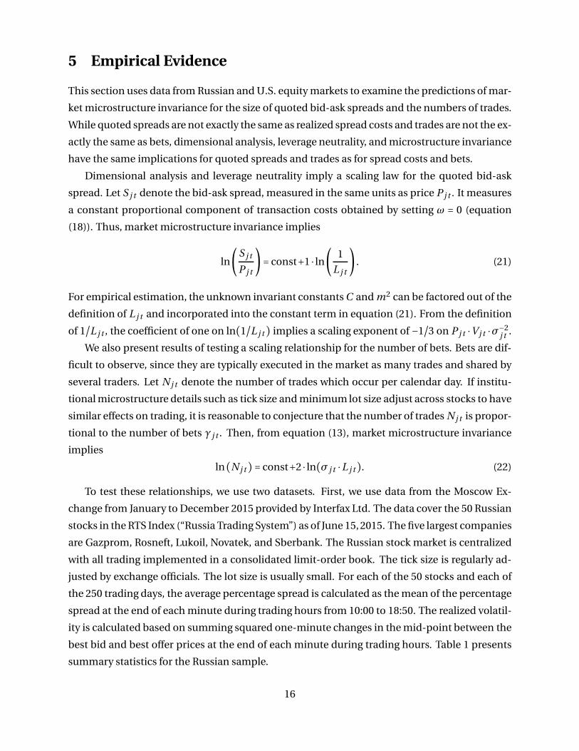
5 Empirical Evidence

This section uses data from Russian and U.S. equity markets to examine the predictions of mar-

ket microstructure invariance for the size of quoted bid-ask spreads and the numbers of trades.

While quoted spreads are not exactly the same as realized spread costs and trades are not the ex-

actly the same as bets, dimensional analysis, leverage neutrality, and microstructure invariance

have the same implications for quoted spreads and trades as for spread costs and bets.

Dimensional analysis and leverage neutrality imply a scaling law for the quoted bid-ask

spread. Let S j t denote the bid-ask spread, measured in the same units as price P j t . It measures

a constant proportional component of transaction costs obtained by setting ω = 0 (equation

(18)). Thus, market microstructure invariance implies

ln(S j t

P j t) = const+1 ⋅ ln( 1

L j t) . (21)

For empirical estimation, the unknown invariant constants C and m2 can be factored out of the

definition of L j t and incorporated into the constant term in equation (21). From the definition

of 1/L j t , the coefficient of one on ln(1/L j t) implies a scaling exponent of −1/3 on P j t ⋅V j t ⋅σ−2j t .

We also present results of testing a scaling relationship for the number of bets. Bets are dif-

ficult to observe, since they are typically executed in the market as many trades and shared by

several traders. Let N j t denote the number of trades which occur per calendar day. If institu-

tional microstructure details such as tick size and minimum lot size adjust across stocks to have

similar effects on trading, it is reasonable to conjecture that the number of trades N j t is propor-

tional to the number of bets γ j t . Then, from equation (13), market microstructure invariance

implies

ln(N j t) = const+2 ⋅ ln(σ j t ⋅L j t). (22)

To test these relationships, we use two datasets. First, we use data from the Moscow Ex-

change from January to December 2015 provided by Interfax Ltd. The data cover the 50 Russian

stocks in the RTS Index (“Russia Trading System”) as of June 15, 2015. The five largest companies

are Gazprom, Rosneft, Lukoil, Novatek, and Sberbank. The Russian stock market is centralized

with all trading implemented in a consolidated limit-order book. The tick size is regularly ad-

justed by exchange officials. The lot size is usually small. For each of the 50 stocks and each of

the 250 trading days, the average percentage spread is calculated as the mean of the percentage

spread at the end of each minute during trading hours from 10:00 to 18:50. The realized volatil-

ity is calculated based on summing squared one-minute changes in the mid-point between the

best bid and best offer prices at the end of each minute during trading hours. Table 1 presents

summary statistics for the Russian sample.

16

Units Avg p5 p50 p95 p100

C ap j t Mkt. Cap. USD Billion 8.76 0.44 3.49 35.02 62.92

C ap j t Mkt. Cap. RUB Billion 476 24 190 1904 3420

V j t ⋅P j t Volume RUB Million/Day 542 3 73 2607 6440

σ j t Volatility 10−4/Day1/2 189 130 180 260 290

S j t /P j t Spread 10−4 20 4 13 66 131

N j t Trades Count/Day 7328 65 2792 22 169 71 960

Table 1: The table presents summary statistics (average values and percentiles) for the sample

of 50 Russian stocks: dollar and ruble capitalization C ap j t (in billions), average daily volume

V j t ⋅P j t in millions of rubles, daily return volatility σ j t , average percentage spread S j t /P j t in

basis points, and average number of trades per day N j t as of June 2015.

Avg p5 p50 p95 p100

C ap j t Mkt. Cap. USD Billion 38 6 18 160 716

V j t ⋅P j t Volume USD Million 205 38 124 591 4647

σ j t Volatility 10−4/Day1/2 110 70 90 160 4050

S j t /P j t Spread 10−4 4 2 3 8 184

N j t Trades 1/Day 21 048 5308 15 735 58 938 190 270

Table 2: The table presents summary statistics (average values and percentiles) for the sample

of 500 U.S. stocks: dollar capitalization C ap j t (in billions), average daily volume V j t ⋅P j t in

millions of dollars, daily return volatilityσ j t , average percentage spread S j t/P j t in basis points,

and average number of trades per day N j t as of June 2015.

Second, we also use daily TAQ (Trade and Quote) data for U.S. stocks from January to De-

cember 2015. The data cover 500 stocks in the S&P 500 index as of June 15, 2015. The largest

companies are Apple, Microsoft, and Exxon Mobil. The U.S. stock market is highly fragmented,

with securities traded simultaneously on dozens of exchanges. For most securities, the mini-

mum tick size is equal to one cent ($0.01), which may be binding for stocks with low price or

high dollar volume. The minimum lot size is usually 100 shares. For each of the 500 stocks and

each of the 252 trading days, the average percentage spread is calculated as the mean of the

percentage spread, based on the best bids and best offers across all exchanges, at the end of

each minute during the hours from 9:30 to 16:00. The realized volatility is calculated based on

summing squared one-minute changes in the mid-point between the best bid and best offer

prices at the end of each minute during trading hours. Table 2 presents summary statistics for

the U.S. sample.

Figure 1 plots the log bid-ask spread ln(S j t /P j t) against ln(1/L j t) using the data from the

Moscow Exchange. Each of 12 426 points represents the average bid-ask spread for each of 50

stocks in the RTS index for each of 250 days. Different colors represent different stocks. For

comparison, we add a solid line ln(S j t /P j t) = 2.112+1⋅ln(1/L j t), where the slope of one is fixed

17

Figure 1: This table plots the bid-ask spread ln(S/P) against illiquidity ln(1/L), with 1/L = (P ⋅V /σ2)−1/3 for each of the 50 Russian stocks in the RTS index for each of 250 days from January

to December 2015.

at the level predicted by market microstructure invariance and the intercept is estimated. All

observations cluster around this benchmark line.

In the aggregate sample, the fitted line is ln(S j t /P j t) = 2.093+0.998 ⋅ ln(1/L j t), with stan-

dard errors of estimates clustered at daily levels equal to 0.040 and 0.005, respectively; the R-

square is 0.876. The invariance prediction that the slope coefficient is one is not statistically

rejected. The fitted line for a similar regression over monthly averages instead of daily averages

is ln(S j t /P j t) = 2.817+1.078 ⋅ ln(1/L j t) with standard errors of estimates 0.164 and 0.019, re-

spectively; its R-square is 0.923. The invariance prediction that the slope coefficient is one is

statistically rejected in this case, but remains economically close to the predicted value.

The 50 dashed lines in figure 1 are fitted based on data for the 50 Russian stocks. The

slopes for individual stocks, which vary from 0.249 to 1.011, are substantially lower than the

invariance-implied slope of one, which is indistinguishable from the fitted line for the aggre-

gate data. Most slope estimates are close to 0.70; ten slope estimates are less than 0.50, and six

slope estimates are larger than 0.90.

Figure 2 plots the log bid-ask spread ln(S j t /P j t) against ln(1/L j t) for the U.S. stocks. Each

of 124 170 points depicts the average bid-ask spread for each of the 500 stocks in the S&P 500 in-

dex and for each of 252 days. As before, different colors represent different stocks. We also add a

solid line ln(S j t /P j t) = 1.371+1 ⋅ ln(1/L j t), where the slope of one is fixed at the level predicted

by market microstructure invariance and only the intercept is estimated. The intercept of 1.371

18

for this sample is smaller than the intercept of 2.112 for the sample of Russian stocks. All ob-

servations again cluster along the benchmark line, even though there are some visible outliers.

The points appear to be more dispersed than in the previous figure.

The fitted line is ln(S j t /P j t) = 1.011+0.961 ⋅ ln(1/L j t) with clustered standard errors of es-

timates being equal to 0.225 and 0.024, respectively, in the aggregate sample; the R-square is

0.450. The invariance prediction that the slope coefficient is one is not statistically rejected.

Depicted with dashed lines, the slopes of 500 fitted lines for 500 individual stocks range from

-0.052 to 1.667. Most of 500 slope estimates lie between 0.90 and 1.30; about 50 stocks have

the slope estimates below 0.50 with the three of them being very close to zero, and about 20 of

stocks have slope estimates higher then 1.50.

The fact that both regressions have a slope close to the predicted value of one indicates that

stock markets in both countries adjust over time so the the invariance relationships hold as ap-

proximations. In both countries, there are economically significant deviations from invariance

in the sense that the R2 of the regressions is less than one. Deviations from invariance may have

different institutional explanations in each country related to minimum tick size and minimum

lot size. In the Russian market, frequent non-uniform adjustments of tick sizes may reduce dis-

tortions associated with tick size restrictions. In the U.S. market, tick size is fixed at the same

level of one cent for most securities, but the tick size as a fraction of the stock price varies when

the stock price changes as a result of market movement or stock splits. The typical large com-

pany has a higher stock price than the typical small company. Stock splits in response to market

movements imply a very slow process for tick size adjustment, and this may lead to more noise

in the invariance relationship estimated for U.S. stocks.

Figure 3 presents results of testing the invariance prediction for the number of trades from

equation (22) using data from the Moscow Exchange. The figure has 12 426 points plotting the

log number of transactions ln(N j t) against ln(σ j t ⋅L j t) for each of 50 stocks and each of 250

days. For comparison with the prediction of invariance, a benchmark line ln(N j t ) = −1.937+

2 ⋅ ln(σ j t ⋅L j t) is added; this line has a slope that is fixed at the predicted level of two and an

intercept that is estimated. The results for the aggregate sample are broadly consistent with

the predictions. The fitted line is ln(N j t) = −3.085+ 2.239 ⋅ ln(σ j t ⋅ L j t) with standard errors

of estimates equal to 0.038 and 0.008, respectively; its R-square is 0.882. As before, the slopes

of fitted lines for individual stocks are systematically lower, ranging from 1.156 to 1.795 and

depicted with dashed lines.

Figure 4 presents results of testing similar prediction (13) for the number of trades N j t using

the data for the U.S. stocks in the S&P 500 index. The figure has 121 760 points plotting the

log number of transactions ln(N j t ) against ln(σ j t ⋅ L j t) for each of 500 U.S. stocks and each

of 252 days. For comparison with the prediction of invariance, a benchmark line ln(N j t) =

19

Figure 2: This table plots the bid-ask spread ln(S/P) against illiquidity ln(1/L), with 1/L = (P ⋅V /σ2)−1/3 for each of the 500 U.S. stocks in the S&P 500 index for each of 252 days from January

to December 2015.

Figure 3: This table plots the number of trades ln(N) against liquidity ln(σ ⋅L) scaled by volatil-

ity σ, with L = (P ⋅V /σ2)1/3 for each of the 50 Russian stocks in the RTS index for each of 250

days from January to December 2015.

20

Figure 4: This table plots the number of trades ln(N) against liquidity ln(σL) scaled by volatility

σ, with L = (P ⋅V /σ2)1/3 for each of the 500 U.S. stocks in the S&P 500 index for each of 250 days

from January to December 2015.

0.251+2 ⋅ ln(σ j t ⋅L j t) is added; this line has a slope that is fixed at the predicted level of two and

an intercept that is estimated. The intercept of 0.251 for the U.S. benchmark line is higher than

the intercept of -1.937 for the Russian benchmark line. Thus, there are approximately e0.251+1.937

or nine times more transactions in the highly fragmented U.S. equity market, possibly reflecting

numerous cross-market arbitrage trades between different trading platforms. The results for

the aggregate sample are broadly consistent with the predicted slope of 2. The fitted line is

ln(N j t ) = 1.005+1.842 ⋅ ln(σ j t ⋅L j t) with standard errors of estimates equal to 0.054 and 0.011,

respectively; its R-square is 0.702.

The slopes of fitted lines for individual stocks, depicted as before with dashed lines, are sys-

tematically lower than predicted, ranging from 0.416 to 2.646 and clustering mostly between

levels of 1.50 and 1.70. The intercepts of the fitted lines for individual stocks also vary substan-

tially, even though basic invariance hypotheses predict that all intercepts must be the same.

We offer several explanations for why the slopes for individual securities are different from

the slopes for the aggregate sample and the slopes predicted by invariance. They may be re-

lated to a combination of econometric issues, economic issues, or conceptual issues. Testing

different hypotheses and assessing their relative importance is an interesting topic which takes

us beyond the scope of this paper.

First, it is possible that a substantial part of the variation in stock-specific measures of liq-

uidity on the right-hand side of the regression equations is due to variations in liquidity of the

21

overall market and therefore may not reflect variations in bid-ask spreads or number of trans-

actions of individual securities. The existence of noise in regressors may bias slope estimates

downwards.

Second, estimates may be biased due to likely correlation between explanatory variables

and error terms. For example, execution of large transactions will mechanically be reflected in

larger volume—and thus a higher liquidity measure—as well as a larger bid-ask spread, since

they are often executed against existing limit orders and liquidity is not replenished instanta-

neously.

Third—and perhaps most importantly—some discrepancies may be explained by differ-

ences in how market frictions such as minimum lot size and minimum tick size affect bid-ask

spreads and trade size. We outline in Section 7 a conceptual approach for adjusting predictions

for these frictions.

6 Methodological Issues

This section re-examines Assumption 1, which states that g(. . .) is correctly specified as a func-

tion of five specific parameters. We first examine whether unnecessary parameters are included

in the model. We then examine whether necessary parameters have been omitted.

Can Our Model be Simplified? Dimensional analysis depends crucially on the set of parame-

ters included. It is possible that we may have initially included some unnecessary parameters

in the model. Suppose that the transaction cost function depends only on four of the hypothe-

sized five parameters, G = g(Q j t ,P j t ,V j t ,σ2j t), and not on the non-intuitive bet cost C .

If so, then dimensional analysis implies that G j t is a function of only one argument, Q j t ⋅

V j t /σ2j t , which is dimensionless but not leverage neutral. Leverage neutrality further implies

that this parameter must be scaled proportionally with leverage, yielding the square root spec-

ification equivalent to equation (20):

G j t = const ⋅σ j t ⋅(∣Q j t ∣V j t)

1/2

. (23)

Without C , the simplified specification mandates a square root model. Pohl et al. (2017) for-

malize this derivation mathematically. Leaving out C thus makes the model very inflexible.

One big advantage of having C in the specification is that it allows nesting linear price im-

pact, bid-ask spreads, and the square root model into one specification governed by the param-

eter ω. Our original analysis is consistent with equilibrium models that imply a linear market

impact.

22

Another subtle but powerful argument favors inclusion of C into the list of arguments. Sup-

pose that one would like to derive a model for the distribution of bet sizes Q j t under the as-

sumption that it may also depend only on the three parameters P j t ,V j t , and σ2j t

, but not C .

Then dimensional analysis implies that the distributions of scaled bet sizes Q j t ⋅σ2j t/V j t are in-

variant. Since the scaled variable is not leverage neutral, it makes this specification inconsistent

with the leverage neutrality assumption. In the last section, we show that inclusion of C into the

list of arguments for bet sizes makes our model more flexible and allows us to circumvent this

problem.

One might think that if the value of C does not vary in all applications of interest, then this

parameter should be dropped from the list of arguments. On the contrary, dimensional analysis

must be based on a complete set of arguments, even though values of some of them are fixed.

Simply omitting these variables, even constant ones, leads to erroneous results. The correct

simplification algorithm is to replace the set of all fixed parameters with a dimensionally in-

dependent subset of themselves and then redo the dimensional analysis, as described in Sonin

(2001). Thus, although the value of C may be fixed in all applications of interest, it should not be

excluded from the original list of parameters since it represents a dimensionally independent

subset of itself. In practice, whether values of bet costs C are indeed fixed remains an empirical

question. If C varies across countries or time periods, then this variable may possibly determine

similarity groups across markets, similar to Reynolds numbers in the turbulence theory.

Sometimes parameters can be eliminated by defining new units. For example, Newton’s

original law of motion says that force is proportional to the product of mass and acceleration,

F ∼ M ⋅ a. If one chooses a force unit such that one unit of force will give unit mass unit ac-

celeration, then the proportionality constant drops out and the equation becomes F = M ⋅ a.

Similarly, if we introduce a new unit of currency equal to the expected cost of executing a bet

(a fundamental unit of money), then C will drop out of all equations. For scientific studies in

market microstructure, this would be a natural unit of currency. Note that since the moment

ratio m is already dimensionless, it is impossible to eliminate it by redefining units.

Could Some Variables Have Been Omitted? It is possible that we may have initially excluded

some necessary parameters. For example, the predictions may hold most closely when mini-

mum tick size is small, minimum lot size is not restrictive, market makers are competitive, and

transaction fees and taxes are minimal. When these assumptions are not met, invariance prin-

ciples provide a benchmark from which the importance of frictions can be measured.

The empirical implications of dimensional analysis, leverage neutrality, and market mi-

crostructure invariance can be generalized to incorporate other variables. Here is a general

methodology for deriving relationships among financial variables, following the Buckingham

23

π-theorem. Suppose we would like to study a variable Y .

• Write down all variables X1, X2, X3, . . . , Xm that may affect Y .

• Construct a dimensionless and leverage-neutral variable αy ⋅Y from Y by scaling it by a

product of powers of X1, . . . , Xm with different exponents, αy = Xy1

1 ⋯Xymm .

• Drop three dimensionally independent arguments used up to make the equation dimen-

sionally consistent and match the dimension of Y , which is made up of the three finance

units. Drop one more argument used up to satisfy a leverage neutrality constraint.

• Scale the remaining arguments X5, . . . , Xm by a product of powers of X1, . . . , Xm with dif-

ferent exponents, αi = X i11 ⋯X im

m for i = 5, . . . ,m to construct dimensionless and leverage-

neutral variables α5 ⋅X5, . . . , αm ⋅Xm .

• Then the resulting equation for Y is αy ⋅Y = f (α5 ⋅X5, . . . ,αm ⋅Xm).This is a generalized algorithm for dimensional analysis and leverage neutrality. It shows

how to include any number of additional explanatory variables into the model.

Including unnecessary parameters does not make a model logically incorrect, but it does

reduce its statistical power by making it unnecessarily complicated. Each new parameter adds

a new variable into a scaling law. If unnecessary variables are included, then extensive empirical

analysis is necessary to show that these parameters are unnecessary.

General Scaling Laws for Market Impact Model. We next derive a more general version of the

market impact model (7) that includes three additional variables. Transaction costs may de-

pend on the execution horizon and market frictions such as minimum tick size and minimum

lot size. The tick size for U.S. stocks is generally one cent, and the minimum round lot size is

generally 100 shares; for Russian stocks there is more variation in these parameters.

First, add to the original five parameters three additional parameters: the horizon of exe-

cution T j t measured in units of time, the minimum tick size K minj t measured in currency per

share, and the minimum round lot size Qminj t

measured in shares. Second, re-scale the new

explanatory variables T j t , K minj t

, and Qminj t

to make them dimensionless and leverage neutral

using the four variables P j t , V j t , σ2j t , and C (including the liquidity variable L j t and the dimen-

sionless moment parameter m). The re-scaled values are T j t ⋅σ2j t⋅L2

j t/m2, K min

j t⋅L j t /P j t , and

Qminj t ⋅σ

2j t ⋅L

2j t/V j t , respectively (up to constants of proportionality). It is convenient to let B j t

denote the scaled execution horizon. Equation (13) for γ j t yields

B j t ∶=T j t ⋅σ2

j t⋅L2

j t

m2=T j t ⋅γ j t . (24)

24

The variable B j t measures the expected number of bets over which a given bet is executed; it

converts clock time to business time.

If minimum tick size and minimum lot size do not affect market impact costs, then the

equation (7) becomes

G j t =1

L j t

⋅ f (Z j t ,B j t) , (25)

where Z j t is scaled bet size defined in equation (4) and B j t is scaled execution time defined in

equation (24).

For example, if price impact is linear in both the size of bets and their rate of execution, then

the market impact model becomes

G j t =1

L j t⋅(λ ⋅Z j t +κ ⋅Z j t /B j t) . (26)

Larger bets executed at a faster rate tend to incur higher transaction costs. This specification

of price impact is derived endogenously in the dynamic model of speculative trading of Kyle,

Obizhaeva and Wang (2017).

More generally, the market impact model (7) generalizes to

G j t =1

L j t⋅ f⎛⎝

P j t ⋅Q j t

C ⋅L j t,

T j t ⋅σ2j t⋅L2

j t

m2;

K minj t⋅L j t

P j t,Qmin

j t⋅σ2

j t⋅L2

j t

V j t

⎞⎠ . (27)

This specification remains consistent with our scaling laws but allows for non-linear relation-

ships among the different arguments of f . Here, the first two arguments are characteristics of a

bet and its execution, and the last two arguments are characteristics of the marketplace. Other

variables can be easily added to the transaction cost model following the same algorithm.

7 Extensions and Other Applications.

Our approach allows us to derive other scaling laws. This flexibility makes it more general than

the approach discussed in Kyle and Obizhaeva (2016c). Next, we present several extensions.

Testing these additional predictions empirically takes us beyond the scope of this paper. We

present them as illustrations of promising directions for future research.

Scaling Laws for Optimal Execution Horizon. Optimal execution horizon is obviously of in-

terest to traders. Suppose that the optimal (cost-minimizing) execution horizon T ∗j t or, alter-

natively, the trading rate ∣Q j t ∣/T ∗j tdepends on the seven variables Q j t , P j t , V j t , σ2

j t, C , K min

j t,

and Qminj t

. When tick size is large, larger quantities available at the best bid and offer prices

25

may make the execution horizon shorter. Execution horizon may also depend on order size in

a non-linear fashion.

Since the ratio ∣Q j t ∣/(V j t ⋅T∗j t) is dimensionless and leverage neutral, the same logic as above

implies that an optimal execution horizon is consistent with a function t∗ of three dimension-

less and leverage neutral parameters:

∣Q j t ∣V j t ⋅T

∗j t

= t∗⎛⎝

P j t ⋅Q j t

C ⋅L j t

;K min

j t ⋅L j t

P j t

,Qmin

j t ⋅σ2j t ⋅L

2j t

V j t

⎞⎠ . (28)

Our analysis does not allow us to place more restrictions on the function t∗. If tick size and

minimum lot size do not affect execution horizon, then the participation rate ∣Q j t ∣/(V j t ⋅T ∗j t)depends only on the first argument of function t∗, the scaled bet size Z j t ∶= P j t ⋅Q j t /(C ⋅L j t)from equation (4): ∣Q j t ∣

V j t ⋅T ∗j t

= t∗(P j t ⋅Q j t

C ⋅L j t) . (29)

If the function t∗ is a constant, then

∣Q j t ∣V j t ⋅T

∗j t

= const. (30)

It is optimal to choose the execution horizon so that traders execute all trades targeting the

same fraction of volume, say one percent of volume until execution of the bet is completed.

Scaling Laws for Optimal Tick Size and Lot Size. Setting optimal tick size and minimum lot

size is of interest for exchange officials and regulators. Let K min∗j t

and Qmin∗j t

denote optimal

tick size and optimal minimum lot size, respectively. Suppose both of them depend on the four

variables P j t , V j t , σ2j t

, and C .

Since the scaled optimal quantities K min∗j t⋅L j t /P j t and Qmin∗

j t⋅L2

j t⋅σ2

j t/V j t are dimensionless

and leverage neutral, the scaling laws for these market frictions can be written as

K min∗j t = const ⋅

P j t

L j t

, Qmin∗j t = const ⋅

V j t

L2j t⋅σ2

j t

. (31)

Since the proportionality constants do not vary across securities, these measures provide good

benchmarks for comparing how restrictive actual tick size and minimum lot size are for differ-

ent securities and across markets.

If traders choose execution horizons T ∗j t

optimally according to equation (28) and exchanges

set tick size K minj t and minimum lot size Qmin

j t at their optimal levels (31), then function f in mar-

ket impact model (27) becomes again a function of only one argument Z j t .

26

Scaling Laws for Bid-Ask Spread. Our approach can be also used to derive more general scal-

ing laws for the bid-ask spread. The bid-ask spread is an integer number of ticks which fluc-

tuates as trading occurs. Let S j t denote the average bid-ask spread, measured in dollars per

share.

Assume the average bid-ask spread depends on the six variables P j t , V j t , σ2j t

, C , K minj t

, and

Qminj t . Re-scale the bid-ask spread as S j t ⋅L j t/P j t to make it dimensionless and leverage neutral.

Then dimensional analysis and leverage neutrality imply that it is a function s of the two re-

scaled dimensionless and leverage-neutral variables K minj t

and Qminj t

:

S j t

P j t

=

1

L j t

⋅ s⎛⎝

K minj t ⋅L j t

P j t

,Qmin

j t ⋅σ2j t ⋅L

2j t

V j t

⎞⎠ . (32)

If tick size and minimum lot size have no influence on bid-ask spreads, then this relationship

simplifies to S j t /P j t ∼ 1/L j t . It is exactly the relationship we have tested above for the Russian

and U.S. equities markets. A promising direction for future research is to examine whether the

R2 in our regression can be improved by estimating an appropriate functional form for s.

Scaling Laws for Margins and Repo Haircuts. Margin requirements determine the amount of

collateral that traders deposit with exchanges or counterparties in order to protect them against

potential losses due to adverse price movements or credit risk. Margin requirements should be

sufficiently large to make losses from default negligible but not so large as to impede financial

transactions.

Repurchase agreements (repo) are a form of over-collateralized borrowing in which a bor-

rower sells a security to a lender with a commitment to buy it back in the future. The repo

haircut is the amount by which the market value of a security exceeds the amount of cash that a

borrower receives. Repo haircuts are similar to margins, because they also protect lenders from

default risks.

Let H j t denote the dollar margin or repo haircut, measured in dollars per share. Suppose

that H j t depends on the seven variables P j t , V j t , σ2j t , C , K min

j t , Qminj t , and horizon T j t . The pa-

rameter T j t reflects the frequency of recalculating margin requirements or repo haircuts as well

as the expected time to detect valuation problems and liquidate collateral. As before, dimen-

sional analysis and leverage neutrality imply that the re-scaled percentage margin H j t ⋅L j t /P j t

is a function h of the three re-scaled dimensionless and leverage-neutral variables K minj t

, Qminj t

,

and T j t :

H j t

P j t

=

1

L j t

⋅h⎛⎝

K minj t ⋅L j t

P j t

,Qmin

j t ⋅σ2j t ⋅L

2j t

V j t

,T j t ⋅σ2

j t ⋅L2j t

m2

⎞⎠ . (33)

27

If minimum tick size, lot size, and collateral liquidation horizon are set optimally, then this

relationship simplifies to H j t /P j t ∼ 1/L j t . The idea that H j t is proportional to 1/L j t captures

the intuition that the optimal haircut depends not only on the standard deviation of returnsσ j t

but also on the speed with which business time operates for the asset. Less liquid assets require

larger haircuts than more liquid assets that are equally safe.

Scaling Laws for Trade Sizes and Number of Trades. Our approach can be also used to derive

more general scaling laws for the distribution of trade sizes and number of trades. Each bet of

size Q j t may be executed as a sequence of smaller trades. Let X j t denote a trade, a fraction of a

bet. Trades and bets have the same units but different underlying economics.

While it is reasonable to conjecture that the size of bets does not depend on minimum tick

size or minimum lot size, the size of trades into which bets are “shredded” is usually affected by

both of these frictions. For example, when tick size is restrictive, there are usually large quanti-

ties available for purchase or sale at best bids and offers; large bets thus may be executed all at

once by cleaning out available bids and offers. It is also known that trades have become so small

in recent years that minimum lot size is often a binding constraint, as shown by Kyle, Obizhaeva

and Tuzun (2016) among others.

Suppose trade size depends on the six variables P j t , V j t , σ2j t

, C , K minj t

, and Qminj t

. Since

P j t ⋅ X j t/(C ⋅ L j t) is dimensionless and leverage neutral, our algorithm leads to the following

scaling laws for the probability distribution of trade sizes X̃ j t :

Prob{P j t ⋅ X̃ j t

C ⋅L j t

< x} = F Xj t

⎛⎝x,

K minj t ⋅L j t

P j t

,Qmin

j t ⋅σ2j t ⋅L

2j t

V j t

⎞⎠ . (34)

Similar scaling laws can be potentially obtained for distributions of bet sizes Q̃ j t , the quantities

at the best bid and offer as well as for depth at tick levels throughout the limit order book.

Let N j t denote the number of trades per day. Then the ratio N j t /γ j t denotes the average

number of trades into which a bet is shredded. Suppose that the number of trades N j t also

depends on the six variables P j t , V j t , σ2j t

, C , K minj t

, and Qminj t

. Following our algorithm, the

number of trades N j t satisfies

N j t =σ2j t ⋅L

2j t ⋅n⎛⎝

K minj t⋅L j t

P j t,Qmin

j t⋅σ2

j t⋅L2

j t

V j t

⎞⎠ . (35)

If the function n() is a constant, implying market frictions do not affect trading strategies of

market participants, we obtain

N j t = const ⋅σ2j t ⋅L

2j t . (36)

28

This is the equation tested earlier using Russian and U.S data. The more general specification

may generate more explanatory power for explaining how the number of trades varies across

stocks.

Conclusion. There is a growing empirical evidence that the scaling laws discussed above match

patterns in financial data, at least approximately. These scaling laws are found in data on trans-

action costs and order size distributions for institutional orders by Kyle and Obizhaeva (2016c);

in data on trades executed in the U.S. and South Korean equities markets by Kyle, Obizhaeva

and Tuzun (2016) and Bae et al. (2016); in Thomson Reuters data on news articles by Kyle et al.

(2014); and in intraday trading patterns of the S&P E-mini futures market by Andersen et al.

(2016).

The ideas discussed in this paper suggest new directions for empirical market microstruc-

ture research. Checking the validity of scaling laws in other samples, identifying boundaries of

their applicability, improving the accuracy of estimates, determining specific functional forms

for f , t∗, s, h∗, F xj t

, n, and the triangulation of proportionality constants are important tasks for

future research.

Our research here is relevant for risk managers and traders, who seek to minimize and mea-

sure market impact costs. It also establishes politically neutral, scientific benchmarks for nu-

merous policy issues connected with market microstructure such as setting tick sizes and min-

imum lot sizes as well as position limits, margin requirements, and repo haircuts. As discussed

in Kyle and Obizhaeva (2016a), such research is highly relevant for the economic analysis of

market crashes like the U.S. stock market “flash crash” of May 2010 examined by the Staffs of

the CFTC and SEC (2010b), the U.S. bond market “flash rally” of October 2014 examined in the

Joint Staff Report (2015), as well as the ruble crash of December 2014 analyzed by Obizhaeva

(2016). Lastly, it directly relates to designing liquidity management tools, one of the central

issues addressed by recent regulatory initiatives.

References

Andersen, Torben G., Oleg Bondarenko, Albert S. Kyle, and Anna A. Obizhaeva. 2016. “Intra-

day Trading Invariance in the E-mini S&P 500 Futures Market.” Working Paper. Available at

SSRN: https://ssrn.com/abstract=2693810.

Bae, Kyoung-hun, Albert S. Kyle, Eun Jung Lee, and Anna A. Obizhaeva. 2016.

“Invariance of Buy-Sell Switching Points.” Working Paper. Available at SSRN:

https://ssrn.com/abstract=2730770.

29

Barenblatt, Grigory Isaakovich. 1996. Scaling, Self-Similarity, and Intermediate Asymptotics.

Cambridge University Press.

Black, Fischer, and Myron Scholes. 1973. “The Pricing of Options and Corporate Liabilities.”

Journal of Political Economy, 81(3): 637–654.

Bouchaud, Jean-Philippe, Doyne J. Farmer, and Fabrizio Lillo. 2009. “How Markets Slowly Di-

gest Changes in Supply and Demand.” In Handbook of Financial Markets: Dynamics and

Evolution. 47–160. North Holland.

Foucault, Thierry, Marco Pagano, and Ailsa Roell. 2013. Market Liquidity: Theory, Evidence,

and Policy. Oxford University Press.

Gabaix, Xavier. 2009. “Power Laws in Economics and Finance.” Annual Review of Economics,

121: 255–293.

Gabaix, Xavier, Parameswaran Gopikrishnan, Vasiliki Plerou, and Eugene H. Stanley.

2003. “A Theory of Power-Law Distributions in Financial Market Fluctuations.” Nature,

423(6937): 267–270.

Gabaix, Xavier, Parameswaran Gopikrishnan, Vasiliki Plerou, and Eugene H. Stanley.

2006. “Institutional Investors and Stock Market Volatility.” Quarterly Journal of Economics,

121(2): 461–504.

Grinold, Richard C., and Ronald N. Kahn. 1995. Active Portfolio Management. Probus Publish-

ing.

Joint Staff Report. 2015. Joint Staff Report: The U.S. Treasury Market on October 15, 2014. Joint

staff report by U.S. Department of the Treasury, Board of Governors of the Federal Reserve

System, Federal Reserve Bank of New York, U.S. Securities and Exchange Commission, U.S.

Commodity Futures Trading Commission. July 13, 2015.

Kolmogorov, Andrey Nikolaevich. 1941. “Local Structure of Turbulence in an Incompressible

Fluid for Very Large Reynolds Numbers.” Dokl. Acad. Nauk SSSR, 31(4): 299–303. Reprinted

in Procedings of the Royal Society London A 434, 9-13, 1991.

Kyle, Albert S. 1985. “Continuous Auctions and Insider Trading.” Econometrica, 53(6): 1315–

1335.

Kyle, Albert S., and Anna A. Obizhaeva. 2016a. “Large Bets and Stock Market Crashes.” Working

Paper. Available at SSRN: https://ssrn.com/abstract=2023776.

30

Kyle, Albert S., and Anna A. Obizhaeva. 2016b. “Market Microstructure Invariance: A Dynamic

Equilibrium Model.” Working Paper. Available at SSRN: https://ssrn.com/abstract=2749531.

Kyle, Albert S., and Anna A. Obizhaeva. 2016c. “Market Microstructure Invariance: Empirical

Hypotheses.” Econometrica, 84(4): 1345–1404.

Kyle, Albert S., Anna A. Obizhaeva, and Tugkan Tuzun. 2016. “Microstructure Invariance

in U.S. Stock Market Trades.” FEDS Working Paper No. 2016-034. Available at SSRN:

https://ssrn.com/abstract=2774039.

Kyle, Albert S., Anna A. Obizhaeva, and Yajun Wang. 2017. “Smooth Trading with

Overconfidence and Market Power.” Review of Economic Studies, Posted March 8:

https://doi.org/10.1093/restud/rdx017.

Kyle, Albert S., Anna A. Obizhaeva, Nitish R. Sinha, and Tugkan Tuzun. 2014.

“News Articles and the Invariance Hypothesis.” Working Paper. Available at SSRN:

https://ssrn.com/abstract=1786124.

Modigliani, Franco, and Merton H. Miller. 1958. “The Cost of Capital, Corporation Finance and

the Theory of Investment.” American Economic Review, 48(3): 261–297.

Newman, M.E.J. 2005. “Power Laws, Pareto Distributions and Zipf’s Law.” Contemporary

Physics, 46(5): 323–351.

Obizhaeva, Anna A. 2016. “The Russian Ruble Crisis of December 2014.” Voprosy Ekonomiki,

5: 66–86.

Pohl, Mathias, Alexander Ristig, Walter Schachermayer, and Ludovic Tangpi. 2017. “The

amazing power of dimensional analysis: Quantifying market impact.” Working Paper. Avail-

able at https://arxiv.org/abs/1702.05434.

Sonin, Ain A. 2001. The Physical Basis of Dimensional Analysis. Cambridge, MA: Department of

Mechanical Engineering, MIT.

Sornette, Didier. 2004. Critical Phenomena in Natural Sciences, Chaos, Fractals, Self-

organization and Disorder: Concepts and Tools. Springer, Heidelberg.

Staffs of the CFTC and SEC. 2010b. Findings Regarding the Market Events of May 6,

2010. Report of the Staffs of the CFTC and SEC to the Joint Advisory Commit-

tee on Emerging Regulatory Issues. September 30, 2010. Final Report. Available at

https://www.sec.gov/news/studies/2010/marketevents-report.pdf.

31