Dimension reduction methods: Algorithmsand Applications

Yousef SaadDepartment of Computer Science

and Engineering

University of Minnesota

University of PaduaJune 7, 2018

Introduction, background, and motivation

Common goal of data mining methods: to extract meaningfulinformation or patterns from data. Very broad area – in-cludes: data analysis, machine learning, pattern recognition,information retrieval, ...

ä Main tools used: linear algebra; graph theory; approximationtheory; optimization; ...

ä In this talk: emphasis on dimension reduction techniquesand the interrelations between techniques

Padua 06/07/18 p. 2

Introduction: a few factoids

ä We live in an era increasingly shaped by ‘DATA’

• ≈ 2.5× 1018 bytes of data created in 2015

• 90 % of data on internet created since 2016

• 3.8 Billion internet users in 2017.

• 3.6 Million Google searches worldwide / minute (5.2 B/day)

• 15.2 Million text messages worldwide / minute

ä Mixed blessing: Opportunities & big challenges.

ä Trend is re-shaping & energizing many research areas ...

ä ... including : numerical linear algebra

Padua 06/07/18 p. 3

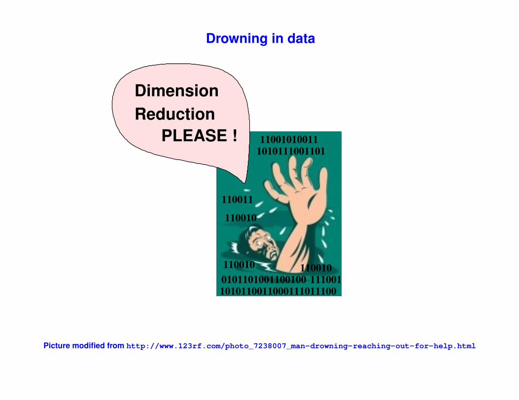
Drowning in data

1010110011000111011100

0101101001100100

11001010011

1010111001101

110010

110011

110010

110010

111001

Dimension

PLEASE !

Reduction

Picture modified from http://www.123rf.com/photo_7238007_man-drowning-reaching-out-for-help.html

Major tool of Data Mining: Dimension reduction

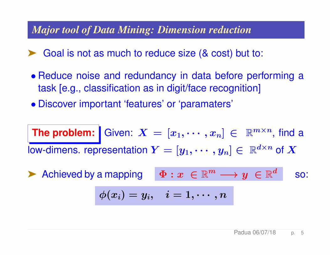
ä Goal is not as much to reduce size (& cost) but to:

• Reduce noise and redundancy in data before performing atask [e.g., classification as in digit/face recognition]

• Discover important ‘features’ or ‘paramaters’

The problem: Given: X = [x1, · · · , xn] ∈ Rm×n, find a

low-dimens. representation Y = [y1, · · · , yn] ∈ Rd×n of X

ä Achieved by a mapping Φ : x ∈ Rm −→ y ∈ Rd so:

φ(xi) = yi, i = 1, · · · , n

Padua 06/07/18 p. 5

m

n

X

Y

x

y

i

id

n

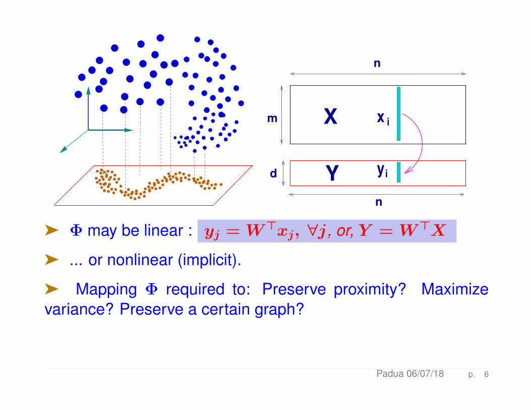
ä Φ may be linear : yj = W>xj, ∀j, or, Y = W>X

ä ... or nonlinear (implicit).

ä Mapping Φ required to: Preserve proximity? Maximizevariance? Preserve a certain graph?

Padua 06/07/18 p. 6

Basics: Principal Component Analysis (PCA)

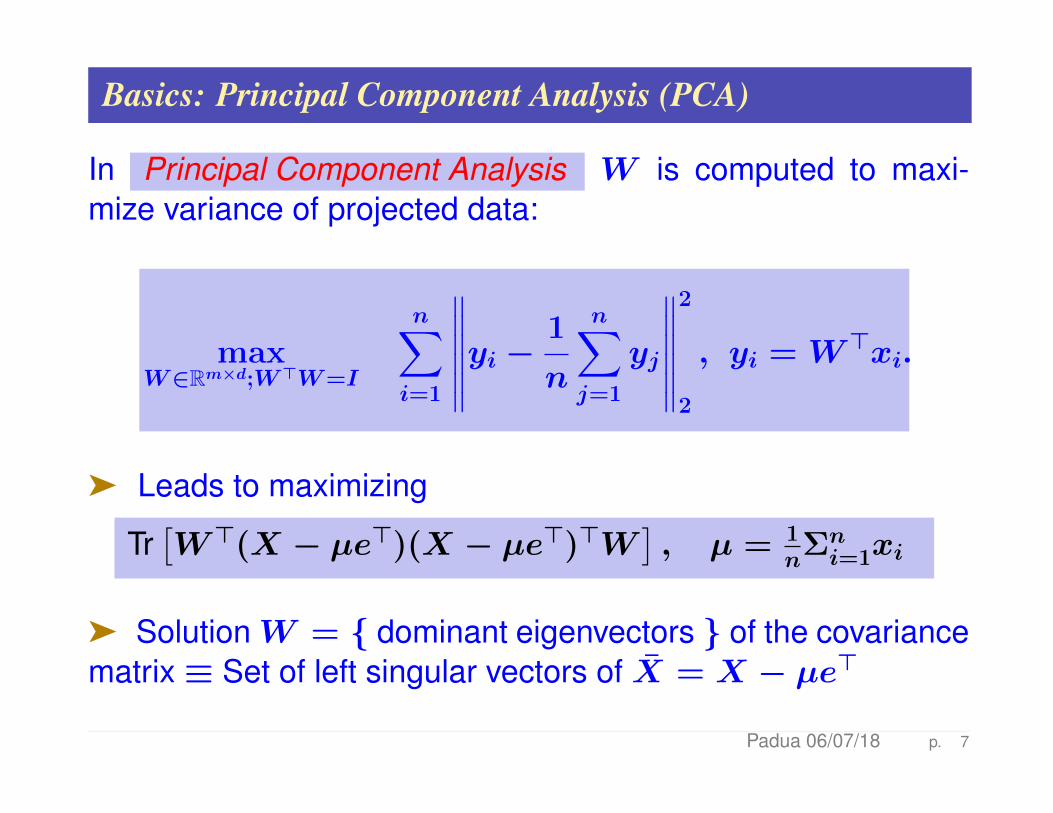
In Principal Component Analysis W is computed to maxi-mize variance of projected data:

maxW∈Rm×d;W>W=I

n∑i=1

∥∥∥∥∥∥yi − 1

n

n∑j=1

yj

∥∥∥∥∥∥2

2

, yi = W>xi.

ä Leads to maximizing

Tr[W>(X − µe>)(X − µe>)>W

], µ = 1

nΣni=1xi

ä SolutionW = { dominant eigenvectors } of the covariancematrix≡ Set of left singular vectors of X = X − µe>

Padua 06/07/18 p. 7

SVD:

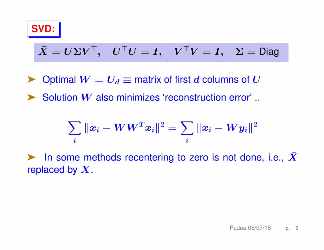
X = UΣV >, U>U = I, V >V = I, Σ = Diag

ä Optimal W = Ud ≡ matrix of first d columns of U

ä Solution W also minimizes ‘reconstruction error’ ..

∑i

‖xi −WW Txi‖2 =∑i

‖xi −Wyi‖2

ä In some methods recentering to zero is not done, i.e., Xreplaced by X.

Padua 06/07/18 p. 8

Unsupervised learning

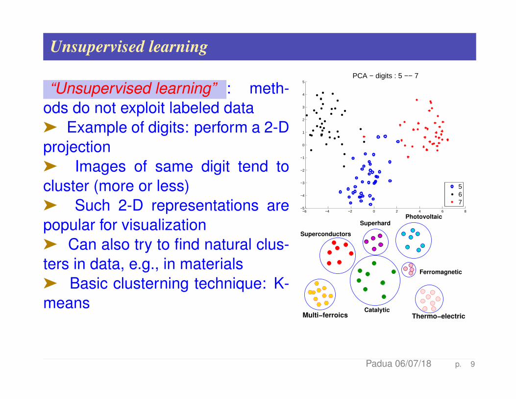
“Unsupervised learning” : meth-ods do not exploit labeled dataä Example of digits: perform a 2-Dprojectionä Images of same digit tend tocluster (more or less)ä Such 2-D representations arepopular for visualizationä Can also try to find natural clus-ters in data, e.g., in materialsä Basic clusterning technique: K-means

−6 −4 −2 0 2 4 6 8−5

−4

−3

−2

−1

0

1

2

3

4

5PCA − digits : 5 −− 7

567

SuperhardPhotovoltaic

Superconductors

Catalytic

Ferromagnetic

Thermo−electricMulti−ferroics

Padua 06/07/18 p. 9

Example: The ‘Swill-Roll’ (2000 points in 3-D)

−15 −10 −5 0 5 10 15−20

−10

0

10

20

−15

−10

−5

0

5

10

15

Original Data in 3−D

Padua 06/07/18 p. 10

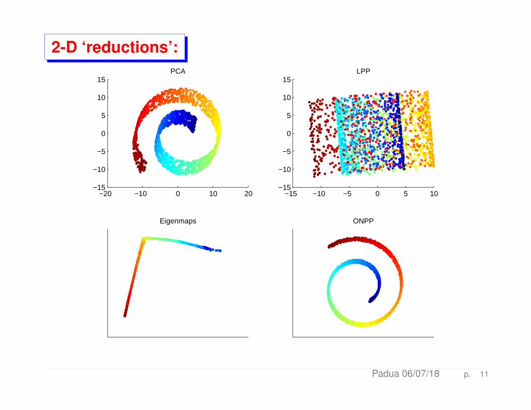
2-D ‘reductions’:

−20 −10 0 10 20−15

−10

−5

0

5

10

15PCA

−15 −10 −5 0 5 10−15

−10

−5

0

5

10

15LPP

Eigenmaps ONPP

Padua 06/07/18 p. 11

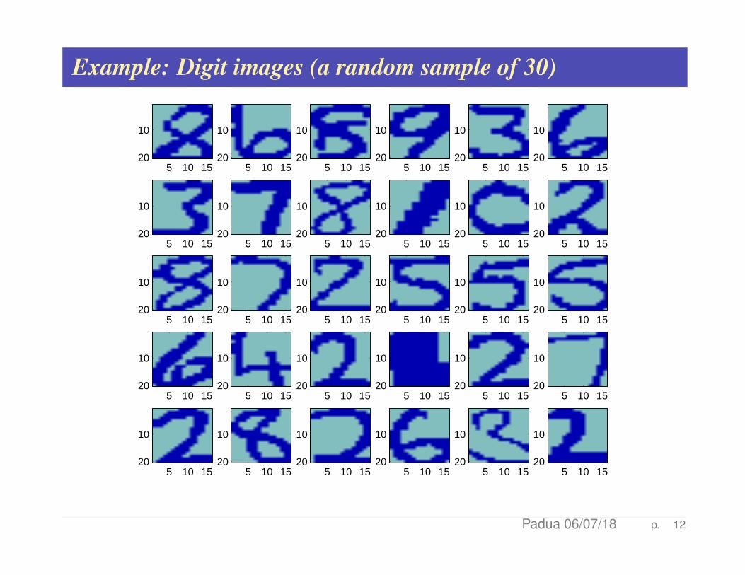
Example: Digit images (a random sample of 30)

5 10 15

10

205 10 15

10

205 10 15

10

205 10 15

10

205 10 15

10

205 10 15

10

20

5 10 15

10

205 10 15

10

205 10 15

10

205 10 15

10

205 10 15

10

205 10 15

10

20

5 10 15

10

205 10 15

10

205 10 15

10

205 10 15

10

205 10 15

10

205 10 15

10

20

5 10 15

10

205 10 15

10

205 10 15

10

205 10 15

10

205 10 15

10

205 10 15

10

20

5 10 15

10

205 10 15

10

205 10 15

10

205 10 15

10

205 10 15

10

205 10 15

10

20

Padua 06/07/18 p. 12

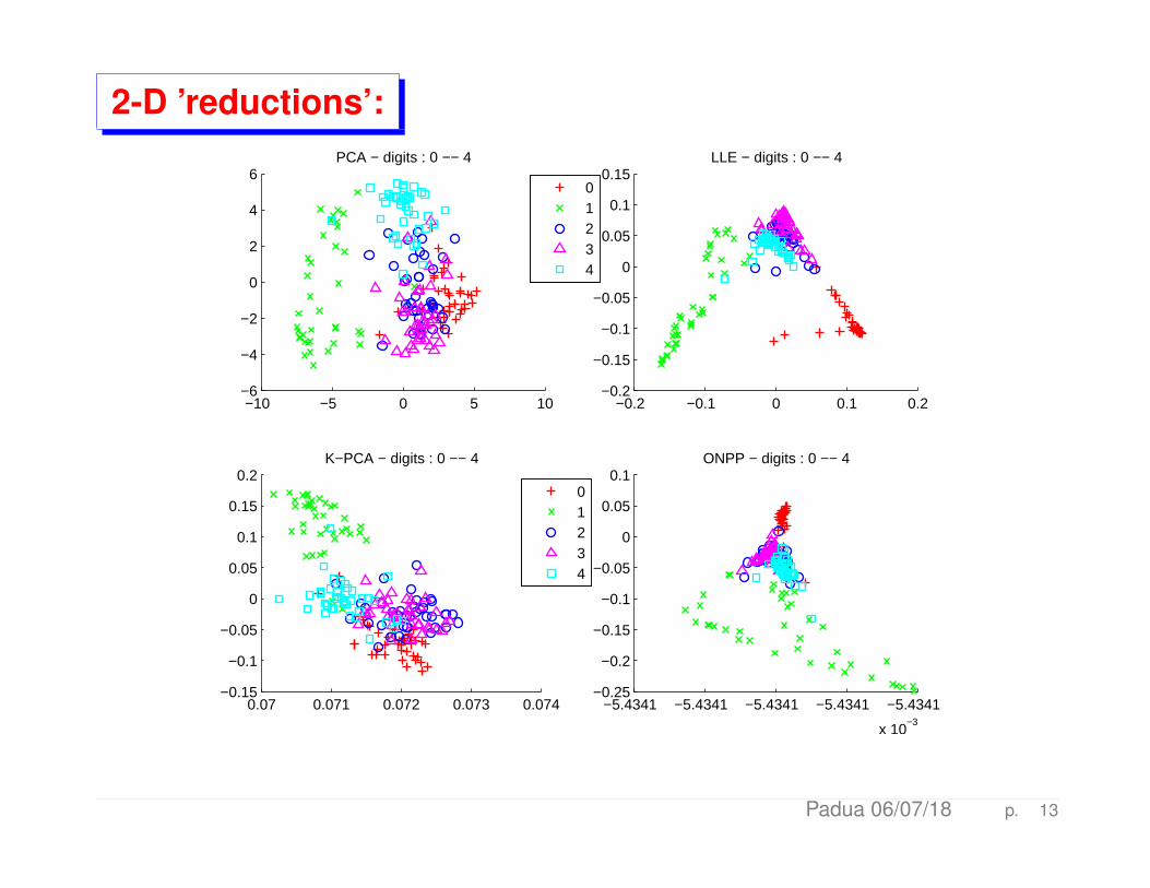
2-D ’reductions’:

−10 −5 0 5 10−6

−4

−2

0

2

4

6PCA − digits : 0 −− 4

01234

−0.2 −0.1 0 0.1 0.2−0.2

−0.15

−0.1

−0.05

0

0.05

0.1

0.15LLE − digits : 0 −− 4

0.07 0.071 0.072 0.073 0.074−0.15

−0.1

−0.05

0

0.05

0.1

0.15

0.2K−PCA − digits : 0 −− 4

01234

−5.4341 −5.4341 −5.4341 −5.4341 −5.4341

x 10−3

−0.25

−0.2

−0.15

−0.1

−0.05

0

0.05

0.1ONPP − digits : 0 −− 4

Padua 06/07/18 p. 13

DIMENSION REDUCTION EXAMPLE: INFORMATION RETRIEVAL

Information Retrieval: Vector Space Model

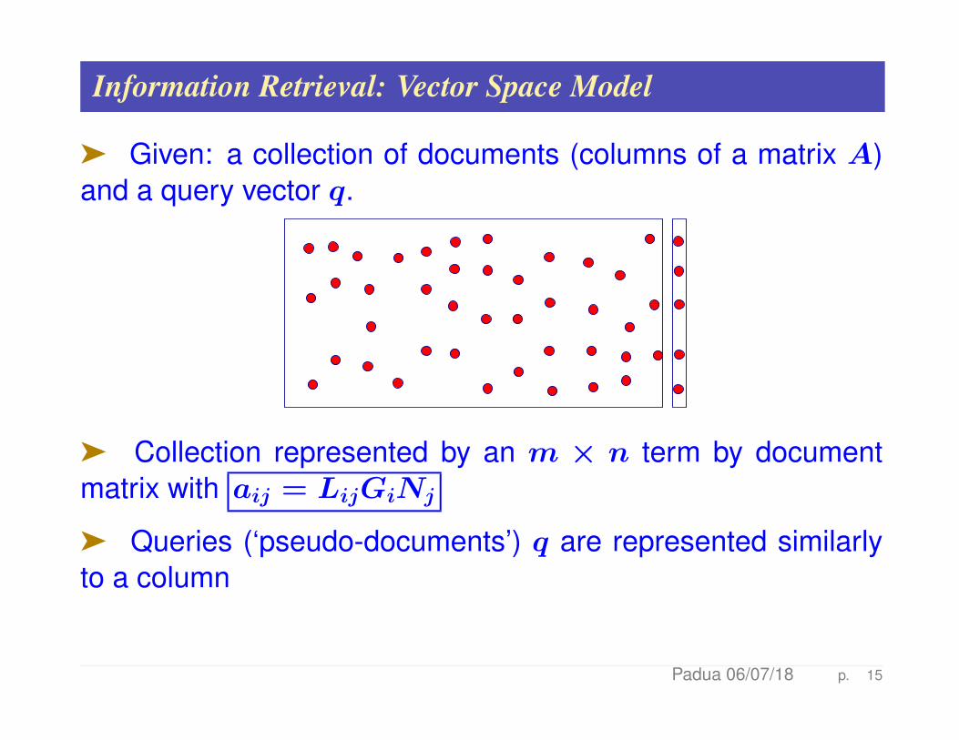
ä Given: a collection of documents (columns of a matrix A)and a query vector q.

ä Collection represented by an m × n term by documentmatrix with aij = LijGiNj

ä Queries (‘pseudo-documents’) q are represented similarlyto a column

Padua 06/07/18 p. 15

Vector Space Model - continued

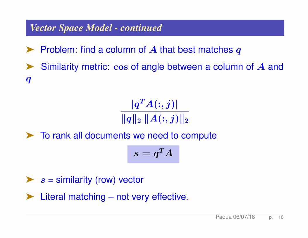
ä Problem: find a column of A that best matches q

ä Similarity metric: cos of angle between a column of A andq

|qTA(:, j)|‖q‖2 ‖A(:, j)‖2

ä To rank all documents we need to compute

s = qTA

ä s = similarity (row) vector

ä Literal matching – not very effective.

Padua 06/07/18 p. 16

Common approach: Use the SVD

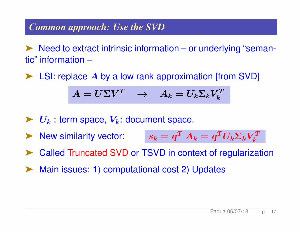
ä Need to extract intrinsic information – or underlying “seman-tic” information –

ä LSI: replace A by a low rank approximation [from SVD]

A = UΣV T → Ak = UkΣkVTk

ä Uk : term space, Vk: document space.

ä New similarity vector: sk = qT Ak = qTUkΣkVTk

ä Called Truncated SVD or TSVD in context of regularization

ä Main issues: 1) computational cost 2) Updates

Padua 06/07/18 p. 17

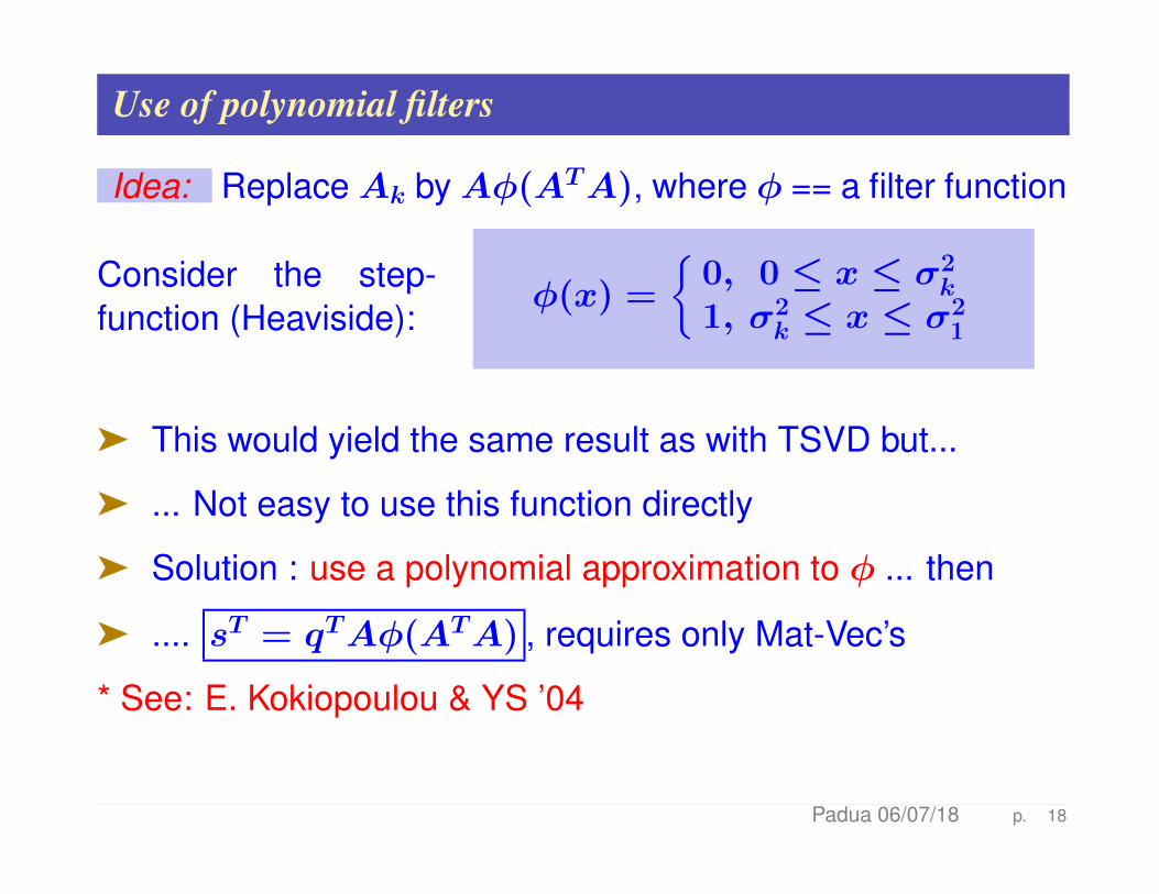
Use of polynomial filters

Idea: ReplaceAk byAφ(ATA), where φ == a filter function

Consider the step-function (Heaviside):

φ(x) =

{0, 0 ≤ x ≤ σ2

k

1, σ2k ≤ x ≤ σ2

1

ä This would yield the same result as with TSVD but...

ä ... Not easy to use this function directly

ä Solution : use a polynomial approximation to φ ... then

ä .... sT = qTAφ(ATA) , requires only Mat-Vec’s

* See: E. Kokiopoulou & YS ’04

Padua 06/07/18 p. 18

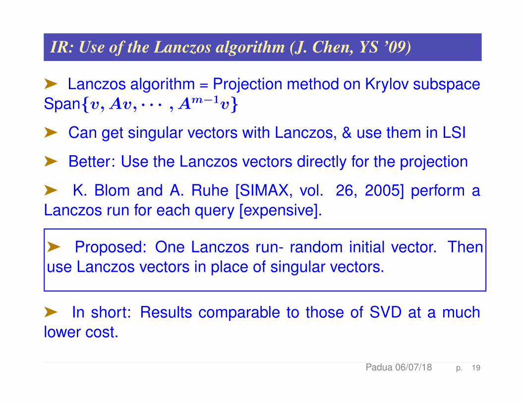
IR: Use of the Lanczos algorithm (J. Chen, YS ’09)

ä Lanczos algorithm = Projection method on Krylov subspaceSpan{v,Av, · · · , Am−1v}

ä Can get singular vectors with Lanczos, & use them in LSI

ä Better: Use the Lanczos vectors directly for the projection

ä K. Blom and A. Ruhe [SIMAX, vol. 26, 2005] perform aLanczos run for each query [expensive].

ä Proposed: One Lanczos run- random initial vector. Thenuse Lanczos vectors in place of singular vectors.

ä In short: Results comparable to those of SVD at a muchlower cost.

Padua 06/07/18 p. 19

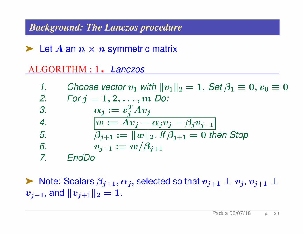
Background: The Lanczos procedure

ä Let A an n× n symmetric matrix

ALGORITHM : 1 Lanczos

1. Choose vector v1 with ‖v1‖2 = 1. Set β1 ≡ 0, v0 ≡ 02. For j = 1, 2, . . . ,m Do:3. αj := vTj Avj4. w := Avj − αjvj − βjvj−1

5. βj+1 := ‖w‖2. If βj+1 = 0 then Stop6. vj+1 := w/βj+1

7. EndDo

ä Note: Scalars βj+1, αj, selected so that vj+1 ⊥ vj, vj+1 ⊥vj−1, and ‖vj+1‖2 = 1.

Padua 06/07/18 p. 20

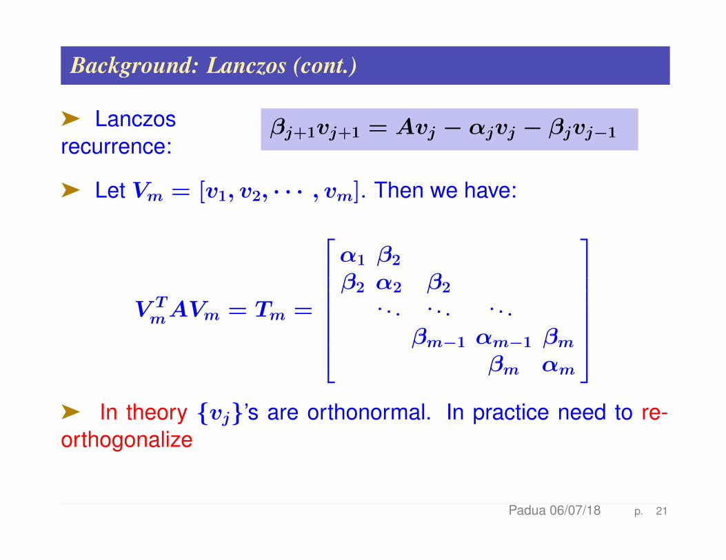
Background: Lanczos (cont.)

ä Lanczosrecurrence:

βj+1vj+1 = Avj − αjvj − βjvj−1

ä Let Vm = [v1, v2, · · · , vm]. Then we have:

V TmAVm = Tm =

α1 β2

β2 α2 β2. . . . . . . . .

βm−1 αm−1 βmβm αm

ä In theory {vj}’s are orthonormal. In practice need to re-orthogonalize

Padua 06/07/18 p. 21

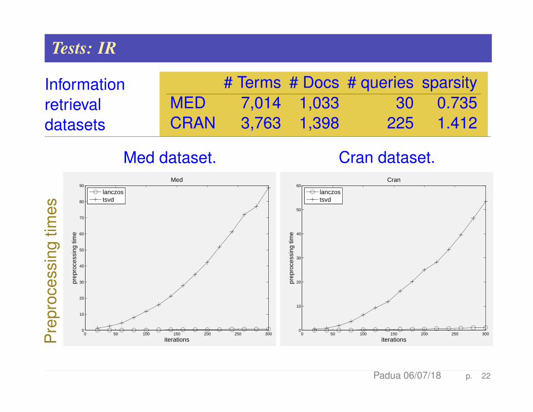
Tests: IR

Informationretrievaldatasets

# Terms # Docs # queries sparsityMED 7,014 1,033 30 0.735CRAN 3,763 1,398 225 1.412

Pre

proc

essi

ngtim

es

Med dataset.

0 50 100 150 200 250 3000

10

20

30

40

50

60

70

80

90Med

iterations

prep

roce

ssin

g tim

e

lanczostsvd

Cran dataset.

0 50 100 150 200 250 3000

10

20

30

40

50

60Cran

iterations

prep

roce

ssin

g tim

e

lanczostsvd

Padua 06/07/18 p. 22

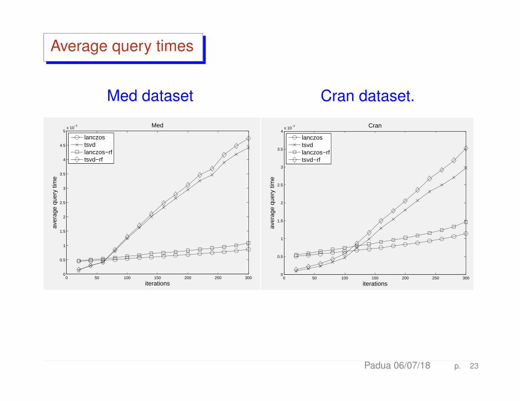
Average query times

Med dataset

0 50 100 150 200 250 3000

0.5

1

1.5

2

2.5

3

3.5

4

4.5

5x 10

−3 Med

iterations

aver

age

quer

y tim

e

lanczostsvdlanczos−rftsvd−rf

Cran dataset.

0 50 100 150 200 250 3000

0.5

1

1.5

2

2.5

3

3.5

4x 10

−3 Cran

iterations

aver

age

quer

y tim

e

lanczostsvdlanczos−rftsvd−rf

Padua 06/07/18 p. 23

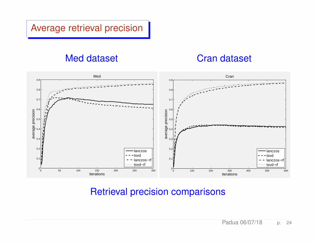
Average retrieval precision

Med dataset

0 50 100 150 200 250 3000

0.1

0.2

0.3

0.4

0.5

0.6

0.7

0.8

0.9Med

iterations

aver

age

prec

isio

n

lanczostsvdlanczos−rftsvd−rf

Cran dataset

0 100 200 300 400 500 6000

0.1

0.2

0.3

0.4

0.5

0.6

0.7

0.8

0.9Cran

iterations

aver

age

prec

isio

n

lanczostsvdlanczos−rftsvd−rf

Retrieval precision comparisons

Padua 06/07/18 p. 24

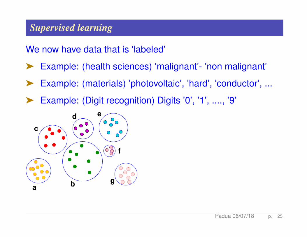
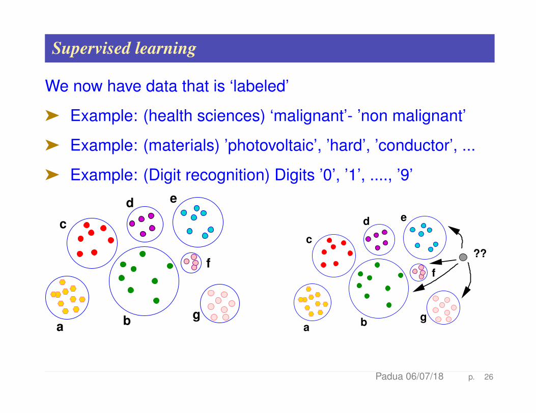
Supervised learning

We now have data that is ‘labeled’

ä Example: (health sciences) ‘malignant’- ’non malignant’

ä Example: (materials) ’photovoltaic’, ’hard’, ’conductor’, ...

ä Example: (Digit recognition) Digits ’0’, ’1’, ...., ’9’

c

e

f

d

a b g

Padua 06/07/18 p. 25

Supervised learning

We now have data that is ‘labeled’

ä Example: (health sciences) ‘malignant’- ’non malignant’

ä Example: (materials) ’photovoltaic’, ’hard’, ’conductor’, ...

ä Example: (Digit recognition) Digits ’0’, ’1’, ...., ’9’

c

e

f

d

a b g

c

e

f

d

a b g

??

Padua 06/07/18 p. 26

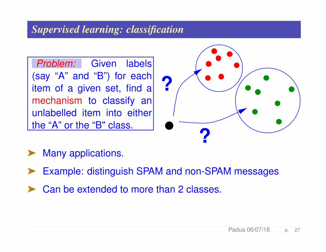
Supervised learning: classification

Problem: Given labels(say “A” and “B”) for eachitem of a given set, find amechanism to classify anunlabelled item into eitherthe “A” or the “B" class.

?

?ä Many applications.

ä Example: distinguish SPAM and non-SPAM messages

ä Can be extended to more than 2 classes.

Padua 06/07/18 p. 27

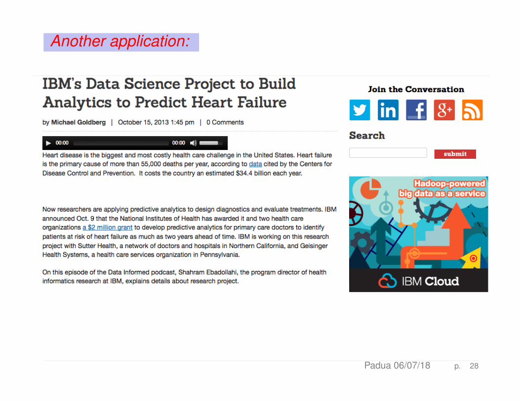
Another application:

Padua 06/07/18 p. 28

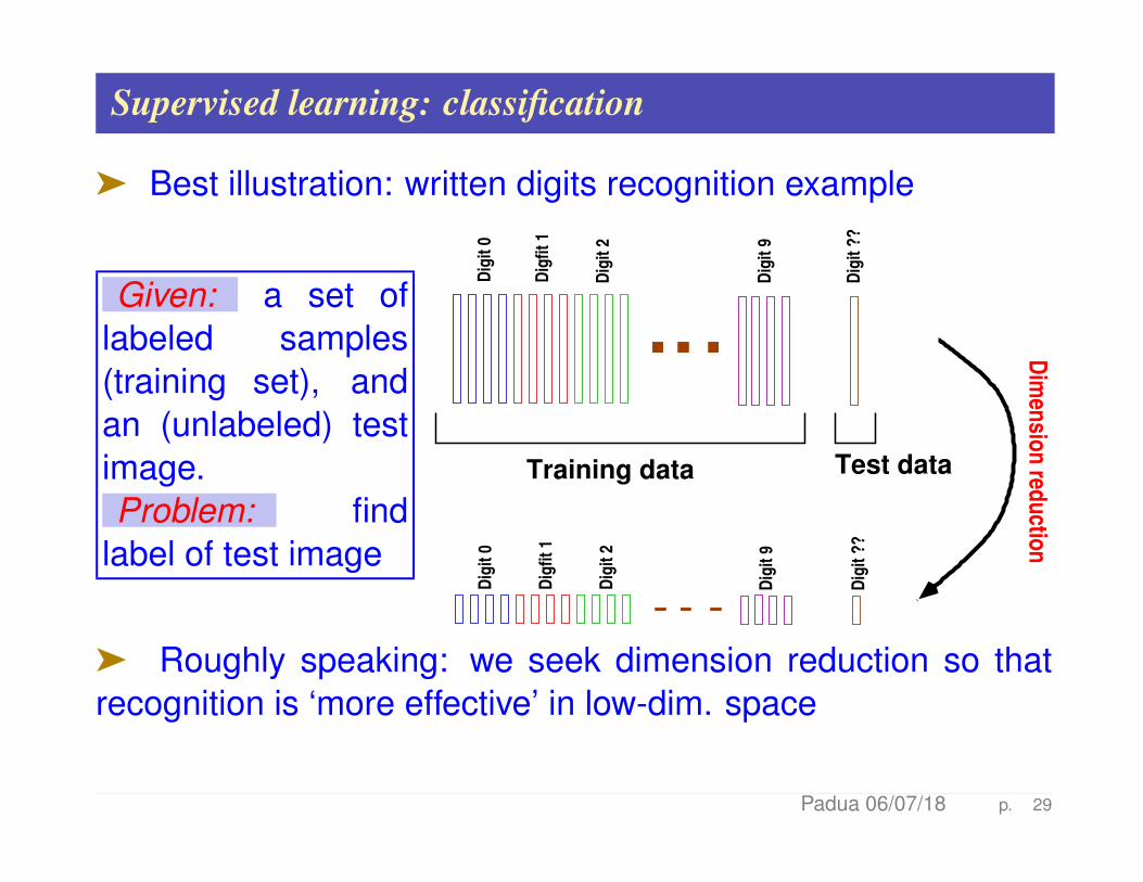
Supervised learning: classification

ä Best illustration: written digits recognition example

Given: a set oflabeled samples(training set), andan (unlabeled) testimage.Problem: find

label of test image

��������

������������

������ ��

Training data Test data

Dim

ensio

n red

uctio

n

Dig

it 0

Dig

fit

1

Dig

it 2

Dig

it 9

Dig

it ?

?

Dig

it 0

Dig

fit

1

Dig

it 2

Dig

it 9

Dig

it ?

?

ä Roughly speaking: we seek dimension reduction so thatrecognition is ‘more effective’ in low-dim. space

Padua 06/07/18 p. 29

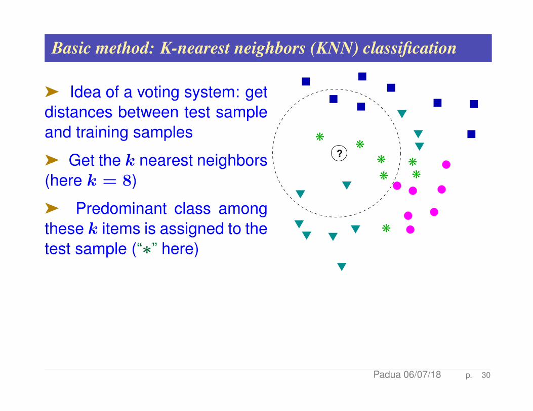
Basic method: K-nearest neighbors (KNN) classification

ä Idea of a voting system: getdistances between test sampleand training samples

ä Get the k nearest neighbors(here k = 8)

ä Predominant class amongthese k items is assigned to thetest sample (“∗” here)

?kk

k k

k

n

n

nn

n

nnn

k

t

t

t

tt

tt

t

t

t

k

Padua 06/07/18 p. 30

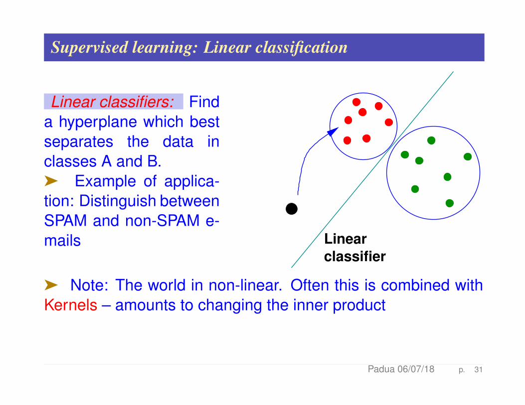
Supervised learning: Linear classification

Linear classifiers: Finda hyperplane which bestseparates the data inclasses A and B.ä Example of applica-tion: Distinguish betweenSPAM and non-SPAM e-mails Linear

classifier

ä Note: The world in non-linear. Often this is combined withKernels – amounts to changing the inner product

Padua 06/07/18 p. 31

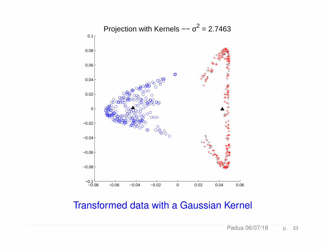
A harder case:

−2 −1 0 1 2 3 4 5−4

−3

−2

−1

0

1

2

3

4Spectral Bisection (PDDP)

ä Use kernels to transform

−0.08 −0.06 −0.04 −0.02 0 0.02 0.04 0.06−0.1

−0.08

−0.06

−0.04

−0.02

0

0.02

0.04

0.06

0.08

0.1

Projection with Kernels −− σ2 = 2.7463

Transformed data with a Gaussian Kernel

Padua 06/07/18 p. 33

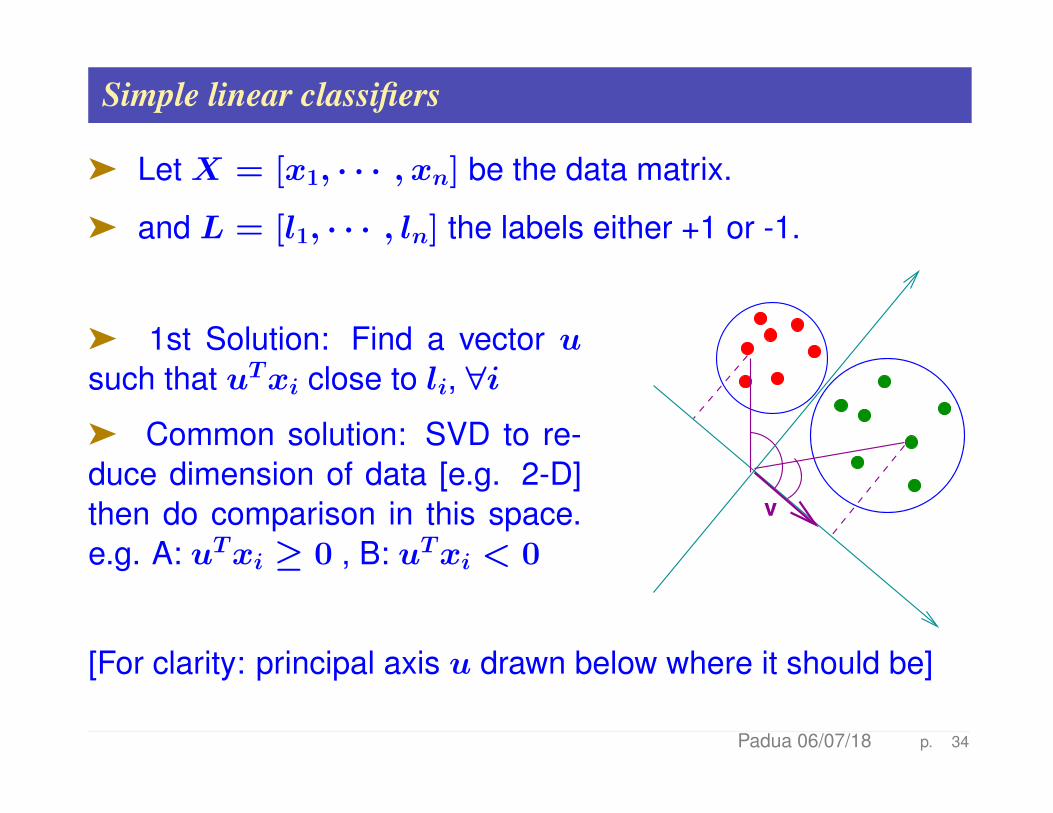
Simple linear classifiers

ä Let X = [x1, · · · , xn] be the data matrix.

ä and L = [l1, · · · , ln] the labels either +1 or -1.

ä 1st Solution: Find a vector usuch that uTxi close to li, ∀iä Common solution: SVD to re-duce dimension of data [e.g. 2-D]then do comparison in this space.e.g. A: uTxi ≥ 0 , B: uTxi < 0

v

[For clarity: principal axis u drawn below where it should be]

Padua 06/07/18 p. 34

Fisher’s Linear Discriminant Analysis (LDA)

Principle: Use label information to build a good projector, i.e.,one that can ‘discriminate’ well between classes

ä Define “between scatter”: a measure of how well separatedtwo distinct classes are.

ä Define “within scatter”: a measure of how well clustereditems of the same class are.

ä Objective: make “between scatter” measure large and “withinscatter” small.

Idea: Find projector that maximizes the ratio of the “betweenscatter” measure over “within scatter” measure

Padua 06/07/18 p. 35

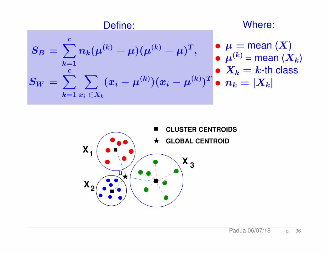
Define:

SB =c∑

k=1

nk(µ(k) − µ)(µ(k) − µ)T ,

SW =c∑

k=1

∑xi ∈Xk

(xi − µ(k))(xi − µ(k))T

Where:

• µ = mean (X)• µ(k) = mean (Xk)• Xk = k-th class• nk = |Xk|

H

GLOBAL CENTROID

CLUSTER CENTROIDS

H

X3

1X

µ

X2

Padua 06/07/18 p. 36

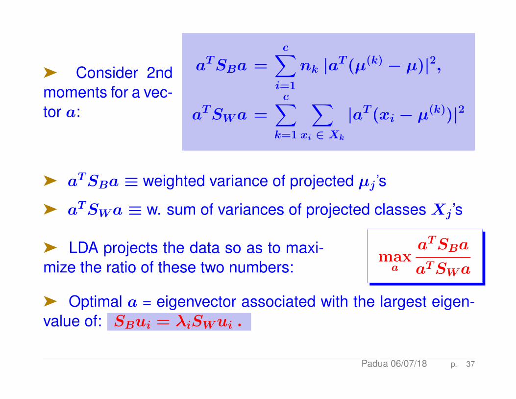
ä Consider 2ndmoments for a vec-tor a:

aTSBa =c∑i=1

nk |aT(µ(k) − µ)|2,

aTSWa =c∑

k=1

∑xi ∈ Xk

|aT(xi − µ(k))|2

ä aTSBa ≡ weighted variance of projected µj’s

ä aTSWa ≡ w. sum of variances of projected classes Xj’s

ä LDA projects the data so as to maxi-mize the ratio of these two numbers:

maxa

aTSBa

aTSWa

ä Optimal a = eigenvector associated with the largest eigen-value of: SBui = λiSWui .

Padua 06/07/18 p. 37

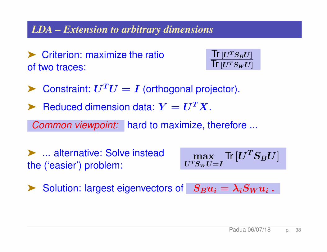
LDA – Extension to arbitrary dimensions

ä Criterion: maximize the ratioof two traces:

Tr [UTSBU ]

Tr [UTSWU ]

ä Constraint: UTU = I (orthogonal projector).

ä Reduced dimension data: Y = UTX.

Common viewpoint: hard to maximize, therefore ...

ä ... alternative: Solve insteadthe (‘easier’) problem:

maxUTSWU=I

Tr [UTSBU ]

ä Solution: largest eigenvectors of SBui = λiSWui .

Padua 06/07/18 p. 38

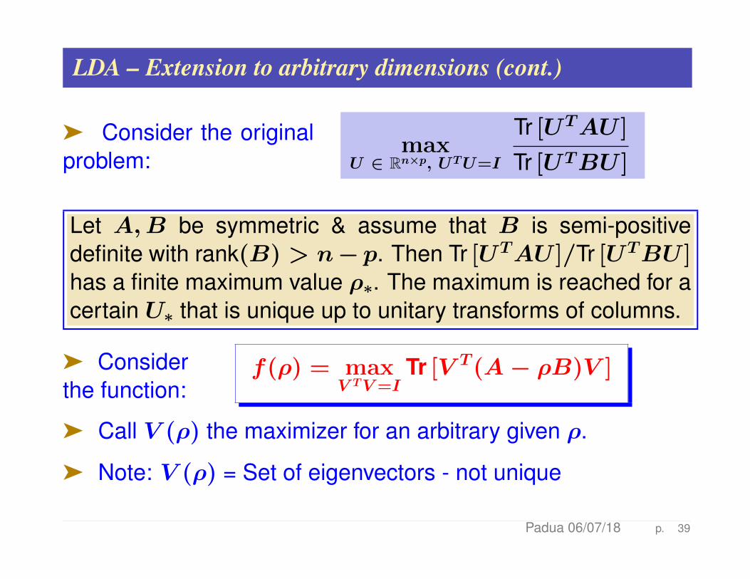
LDA – Extension to arbitrary dimensions (cont.)

ä Consider the originalproblem:

maxU ∈ Rn×p, UTU=I

Tr [UTAU ]

Tr [UTBU ]

Let A,B be symmetric & assume that B is semi-positivedefinite with rank(B) > n− p. Then Tr [UTAU ]/Tr [UTBU ]has a finite maximum value ρ∗. The maximum is reached for acertain U∗ that is unique up to unitary transforms of columns.

ä Considerthe function:

f(ρ) = maxV TV=I

Tr [V T(A− ρB)V ]

ä Call V (ρ) the maximizer for an arbitrary given ρ.

ä Note: V (ρ) = Set of eigenvectors - not unique

Padua 06/07/18 p. 39

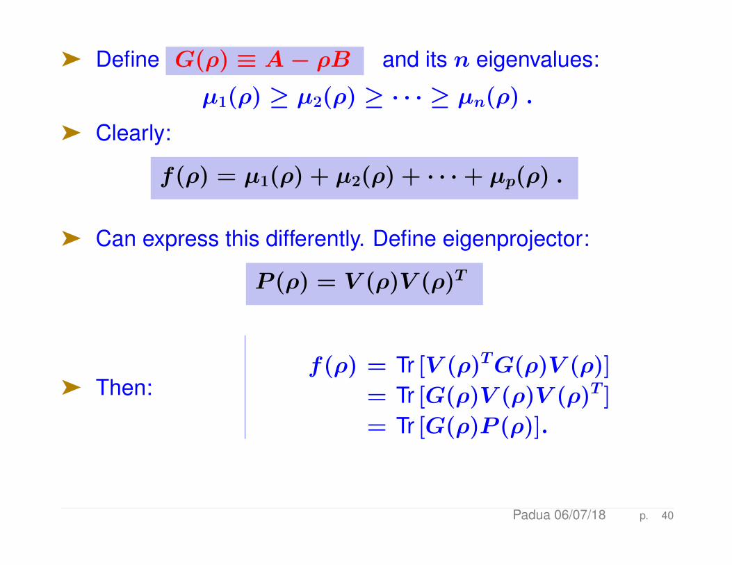
ä Define G(ρ) ≡ A− ρB and its n eigenvalues:

µ1(ρ) ≥ µ2(ρ) ≥ · · · ≥ µn(ρ) .

ä Clearly:

f(ρ) = µ1(ρ) + µ2(ρ) + · · ·+ µp(ρ) .

ä Can express this differently. Define eigenprojector:

P (ρ) = V (ρ)V (ρ)T

ä Then:f(ρ) = Tr [V (ρ)TG(ρ)V (ρ)]

= Tr [G(ρ)V (ρ)V (ρ)T ]

= Tr [G(ρ)P (ρ)].

Padua 06/07/18 p. 40

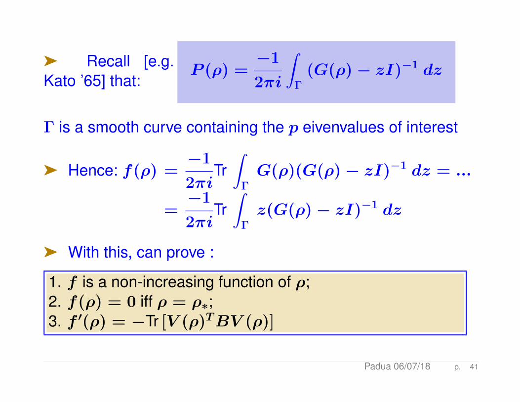
ä Recall [e.g.Kato ’65] that:

P (ρ) =−1

2πi

∫Γ

(G(ρ)− zI)−1 dz

Γ is a smooth curve containing the p eivenvalues of interest

ä Hence: f(ρ) =−1

2πiTr∫

ΓG(ρ)(G(ρ)− zI)−1 dz = ...

=−1

2πiTr∫

Γz(G(ρ)− zI)−1 dz

ä With this, can prove :

1. f is a non-increasing function of ρ;2. f(ρ) = 0 iff ρ = ρ∗;3. f ′(ρ) = −Tr [V (ρ)TBV (ρ)]

Padua 06/07/18 p. 41

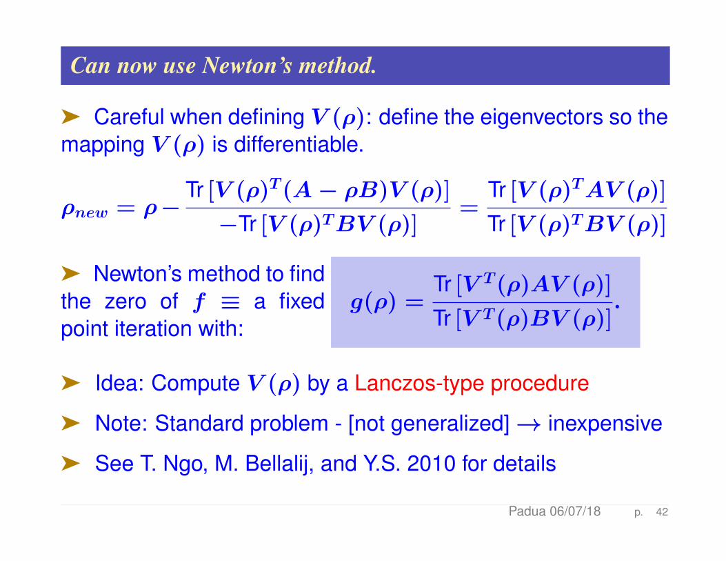
Can now use Newton’s method.

ä Careful when defining V (ρ): define the eigenvectors so themapping V (ρ) is differentiable.

ρnew = ρ−Tr [V (ρ)T(A− ρB)V (ρ)]

−Tr [V (ρ)TBV (ρ)]=

Tr [V (ρ)TAV (ρ)]

Tr [V (ρ)TBV (ρ)]

ä Newton’s method to findthe zero of f ≡ a fixedpoint iteration with:

g(ρ) =Tr [V T(ρ)AV (ρ)]

Tr [V T(ρ)BV (ρ)].

ä Idea: Compute V (ρ) by a Lanczos-type procedure

ä Note: Standard problem - [not generalized]→ inexpensive

ä See T. Ngo, M. Bellalij, and Y.S. 2010 for details

Padua 06/07/18 p. 42

GRAPH-BASED TECHNIQUES

Multilevel techniques in brief

ä Divide and conquer paradigms as well as multilevel methodsin the sense of ‘domain decomposition’

ä Main principle: very costly to do an SVD [or Lanczos] onthe whole set. Why not find a smaller set on which to do theanalysis – without too much loss?

ä Tools used: graph coarsening, divide and conquer –

ä For text data we use hypergraphs

Padua 06/07/18 p. 44

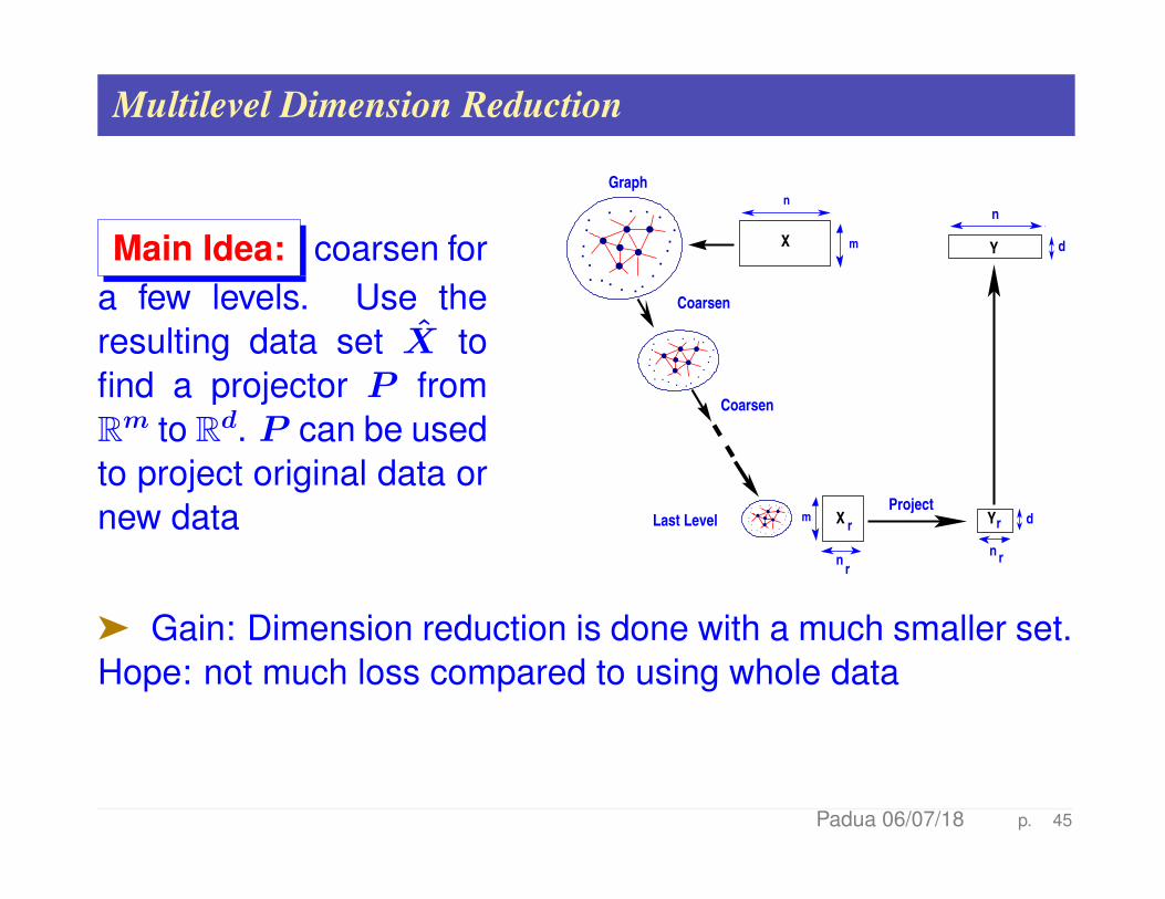
Multilevel Dimension Reduction

Main Idea: coarsen fora few levels. Use theresulting data set X tofind a projector P fromRm to Rd. P can be usedto project original data ornew data

l

l l

ll

l.

.

.

.

. .

.

.

.

.

.

.

.

..

. .

.

.

.

l

l l

ll

l.

.

.

.

. .

.

.

.

.

.

.

.

..

. .

.

.

.

l

l ll

l

l.

.

.

.

. .

.

.

.

.

.

.

.

..

. .

.

.

.

dY

n

Y

n

d

r

r

Coarsen

Coarsen

Graphn

mX

Last Level Xm

nr

r

Project

ä Gain: Dimension reduction is done with a much smaller set.Hope: not much loss compared to using whole data

Padua 06/07/18 p. 45

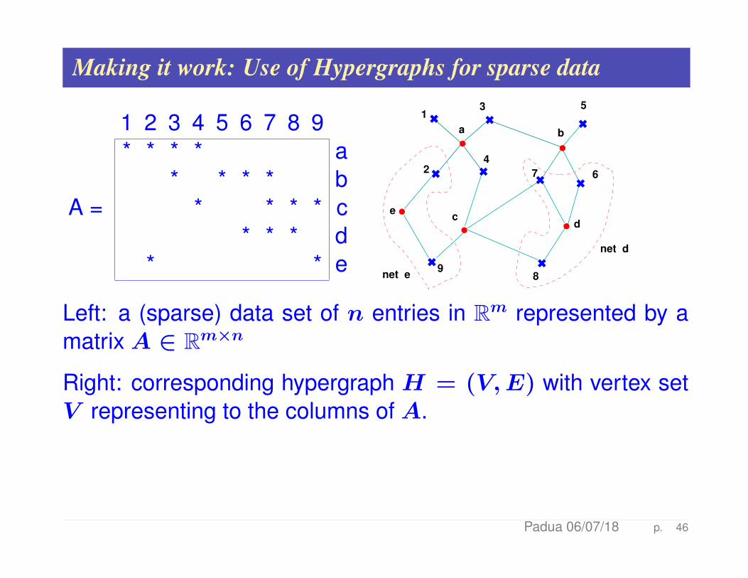
Making it work: Use of Hypergraphs for sparse data

1 2 3 4 5 6 7 8 9* * * * a

* * * * bA = * * * * c

* * * d* * e

6 6

l

6 6

l

ll

6

66

66

l

1

2

3

4

5

67

89

a b

cd

e

net e

net d

Left: a (sparse) data set of n entries in Rm represented by amatrix A ∈ Rm×n

Right: corresponding hypergraph H = (V,E) with vertex setV representing to the columns of A.

Padua 06/07/18 p. 46

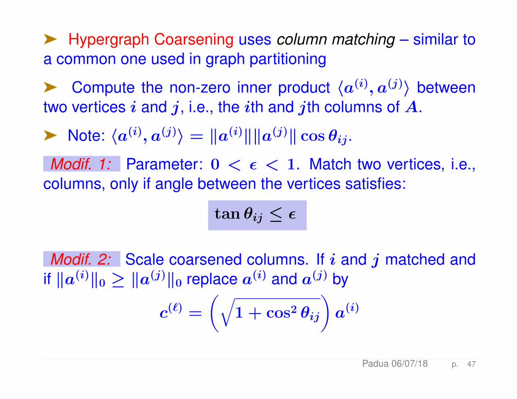
ä Hypergraph Coarsening uses column matching – similar toa common one used in graph partitioning

ä Compute the non-zero inner product 〈a(i), a(j)〉 betweentwo vertices i and j, i.e., the ith and jth columns of A.

ä Note: 〈a(i), a(j)〉 = ‖a(i)‖‖a(j)‖ cos θij.

Modif. 1: Parameter: 0 < ε < 1. Match two vertices, i.e.,columns, only if angle between the vertices satisfies:

tan θij ≤ ε

Modif. 2: Scale coarsened columns. If i and j matched andif ‖a(i)‖0 ≥ ‖a(j)‖0 replace a(i) and a(j) by

c(`) =

(√1 + cos2 θij

)a(i)

Padua 06/07/18 p. 47

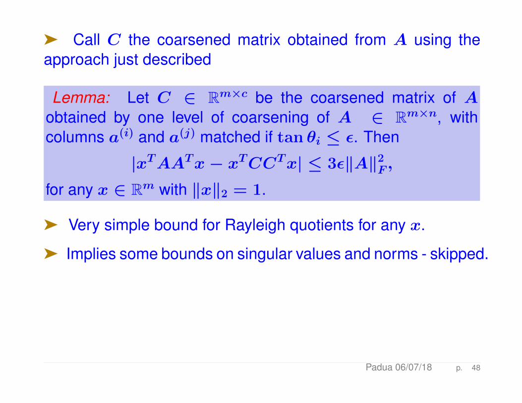
ä Call C the coarsened matrix obtained from A using theapproach just described

Lemma: Let C ∈ Rm×c be the coarsened matrix of Aobtained by one level of coarsening of A ∈ Rm×n, withcolumns a(i) and a(j) matched if tan θi ≤ ε. Then

|xTAATx− xTCCTx| ≤ 3ε‖A‖2F ,

for any x ∈ Rm with ‖x‖2 = 1.

ä Very simple bound for Rayleigh quotients for any x.

ä Implies some bounds on singular values and norms - skipped.

Padua 06/07/18 p. 48

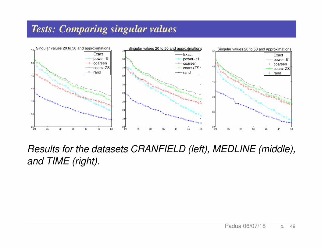
Tests: Comparing singular values

20 25 30 35 40 45 5025

30

35

40

45

50

55

Exactpower−it1coarsencoars+ZSrand

Singular values 20 to 50 and approximations

20 25 30 35 40 45 5020

22

24

26

28

30

32

34

36

38

Exactpower−it1coarsencoars+ZSrand

Singular values 20 to 50 and approximations

20 25 30 35 40 45 5025

30

35

40

45

50

Exactpower−it1coarsencoars+ZSrand

Singular values 20 to 50 and approximations

Results for the datasets CRANFIELD (left), MEDLINE (middle),and TIME (right).

Padua 06/07/18 p. 49

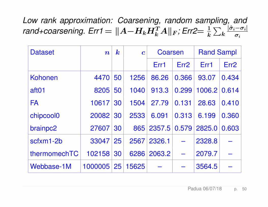
Low rank approximation: Coarsening, random sampling, andrand+coarsening. Err1 = ‖A−HkH

TkA‖F ; Err2= 1

k

∑k|σi−σi|σi

Dataset n k c Coarsen Rand Sampl

Err1 Err2 Err1 Err2

Kohonen 4470 50 1256 86.26 0.366 93.07 0.434

aft01 8205 50 1040 913.3 0.299 1006.2 0.614

FA 10617 30 1504 27.79 0.131 28.63 0.410

chipcool0 20082 30 2533 6.091 0.313 6.199 0.360

brainpc2 27607 30 865 2357.5 0.579 2825.0 0.603

scfxm1-2b 33047 25 2567 2326.1 – 2328.8 –

thermomechTC 102158 30 6286 2063.2 – 2079.7 –

Webbase-1M 1000005 25 15625 – – 3564.5 –

Padua 06/07/18 p. 50

LINEAR ALGEBRA METHODS: EXAMPLES

Updating the SVD (E. Vecharynski and YS’13)

ä In applications, data matrix X often updated

ä Example: Information Retrieval (IR), can add documents,add terms, change weights, ..

Problem

Given the partial SVD of X, how to get a partial SVD of Xnew

ä Will illustrate only with update of the form Xnew = [X,D](documents added in IR)

Padua 06/07/18 p. 52

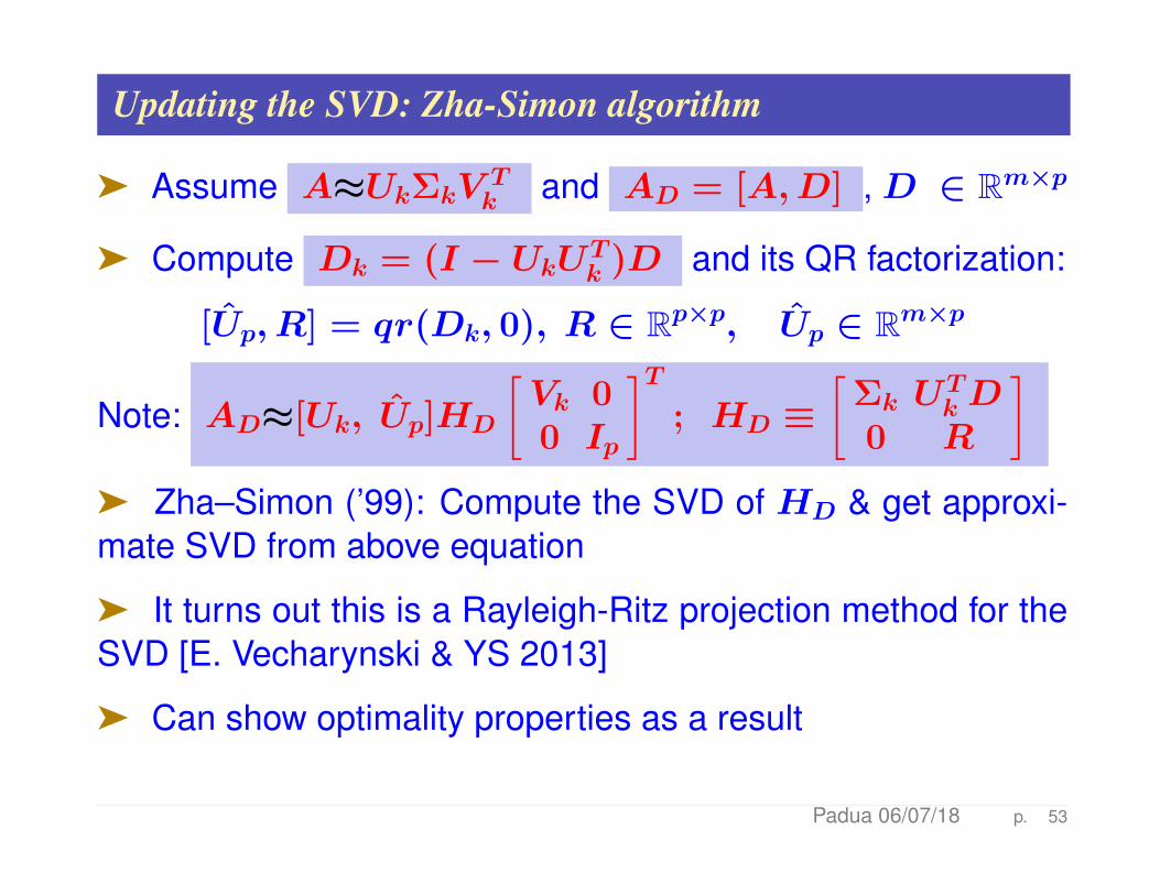
Updating the SVD: Zha-Simon algorithm

ä Assume A≈UkΣkVTk and AD = [A,D] , D ∈ Rm×p

ä Compute Dk = (I − UkUTk )D and its QR factorization:

[Up, R] = qr(Dk, 0), R ∈ Rp×p, Up ∈ Rm×p

Note: AD≈[Uk, Up]HD

[Vk 00 Ip

]T; HD ≡

[Σk U

TkD

0 R

]ä Zha–Simon (’99): Compute the SVD of HD & get approxi-mate SVD from above equation

ä It turns out this is a Rayleigh-Ritz projection method for theSVD [E. Vecharynski & YS 2013]

ä Can show optimality properties as a result

Padua 06/07/18 p. 53

Updating the SVD

ä When the number of updates is large this becomes costly.

ä Idea: Replace Up by a low dimensional approximation:

ä Use U of the form U = [Uk, Zl] instead of U = [Uk, Up]

ä Zl must capture the range of Dk = (I − UkUTk )D

ä Simplest idea : best rank–l approximation using the SVD.

ä Can also use Lanczos vectors from the Golub-Kahan-Lanczosalgorithm.

Padua 06/07/18 p. 54

An example

ä LSI - with MEDLINE collection: m = 7, 014 (terms), n =1, 033 (docs), k = 75 (dimension), t = 533 (initial # docs),nq = 30 (queries)

ä Adding blocks of 25 docs at a time

ä The number of singular triplets of (I−UkUTk )D using SVD

projection (“SV”) is 2.

ä For GKL approach (“GKL”) 3 GKL vectors are used

ä These two methods are compared to Zha-Simon (“ZS”).

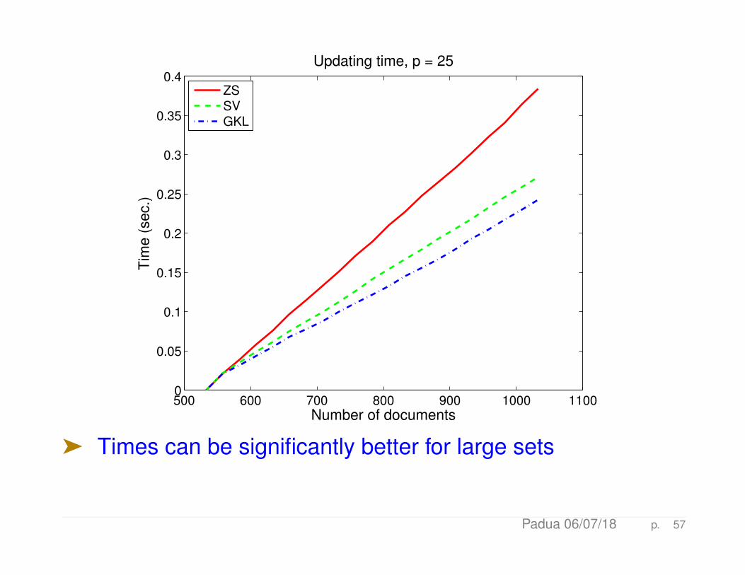
ä We show average precision then time

Padua 06/07/18 p. 55

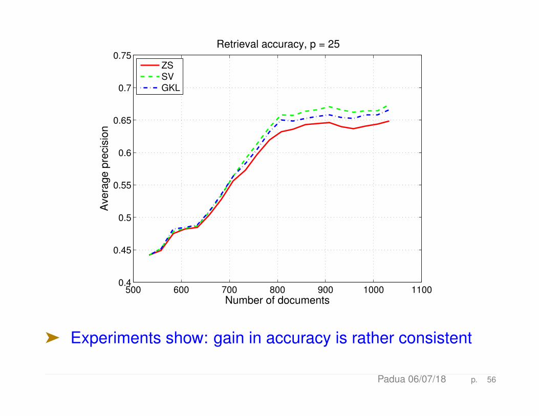
500 600 700 800 900 1000 11000.4

0.45

0.5

0.55

0.6

0.65

0.7

0.75

Avera

ge p

recis

ion

Number of documents

Retrieval accuracy, p = 25

ZS

SV

GKL

ä Experiments show: gain in accuracy is rather consistent

Padua 06/07/18 p. 56

500 600 700 800 900 1000 11000

0.05

0.1

0.15

0.2

0.25

0.3

0.35

0.4

Tim

e (

se

c.)

Updating time, p = 25

Number of documents

ZS

SV

GKL

ä Times can be significantly better for large sets

Padua 06/07/18 p. 57

Conclusion

ä Interesting new matrix problems in areas that involve theeffective mining of data

ä Among the most pressing issues is that of reducing compu-tational cost - [SVD, SDP, ..., too costly]

ä Many online resources available

ä Huge potential in areas like materials science though inertiahas to be overcome

ä To a researcher in computational linear algebra : big tide ofchange on types or problems, algorithms, frameworks, culture,..

ä But change should be welcome

When one door closes, another opens; but we often look solong and so regretfully upon the closed door that we do notsee the one which has opened for us.

Alexander Graham Bell (1847-1922)

ä In the words of Lao Tzu:

If you do not change directions, you may end-up where youare heading

Thank you !

ä Visit my web-site at www.cs.umn.edu/~saad

Padua 06/07/18 p. 59