DIGITAL IMAGING SYSTEM TESTING AND DESIGN USING PHYSICAL

SENSOR CHARACTERISTICS

by

Brent McCleary

A Dissertation Presented to the

FACULTY OF THE GRADUATE SCHOOL

UNIVERSITY OF SOUTHERN CALIFORNIA

In Partial Fulfillment of the

Requirements for the Degree

DOCTOR OF PHILOSOPHY

(ELECTRICAL ENGINEERING)

December 2009

Copyright 2009 Brent McCleary

ii

Dedication

To my family and in memory of my father.

iii

Acknowledgements

I would like to express my sincere gratitude to my advisor, Prof. Antonio Ortega, for his

guidance and patience during my long journey in pursuit of my Ph.D. degree at the

University of Southern California. The support and encouragement I received from Prof.

Ortega were invaluable. I would like to thank Prof. Richard Leahy and Prof. Aiichiro

Nakano for serving as members in my dissertation committee. The time that Prof. Leahy

spent in providing advice on my work is greatly appreciated. I would also like to thank

Prof. Alexander A. Sawchuk and Prof. C.-C. Jay Kuo for being members of my qualifying

exam committee. It was a great privilege to receive their valuable guidance on my work.

In addition, I would like to thank the many people who provided helpful advice,

valuable information, and feedback on my work. In particular, I thank In Suk Chong,

Quanzheng Li, and Jim Janesick. I also thank Diane Demetras for all of the help that

she has provided to me over the years.

I wish to express my deepest gratitude to my lovely wife Leigh. I would be lost

without her support and love. I thank my sons, Xanden and Xealen, for their optimism.

I thank my late father, George, my mother, Marigold, and my sister, Maxene, for their

unconditional love.

iv

Table of Contents

Dedication ii Acknowledgements iii List of Tables vii List of Figures viii Abstract xiv Chapter 1 Introduction 1

1.1 Pixel Response Non-Uniformity 2 1.2 Bayer Cross-Talk Problem 3 1.3 Contributions of the Research 5

1.3.1 Contributions of Pixel Response Non-Uniformity Testing Method 5

1.3.2 Contributions of Bayer Cross-Talk Solution 6 Chapter 2 Photo-Response Non-Uniformity Error Testing Methodology for

CMOS Imager Systems 8 2.1 Introduction 8 2.2 Background on CMOS PRNU Defects 9

2.2.1 Image Sensor Pixel Defects 9 2.2.1.1 Causes of PRNU 10 2.2.1.2 Hot and Cold Pixel Defects 12

2.2.2 Reasons for Studying PRNU Defect Testing 12 2.2.3 PRNU Characterization 13 2.2.4 Industry Standard PRNU Screening 14 2.2.5 PRNU Screening Metric Behavior 17 2.2.6 Typical Sensor Values of PRNU 20

2.3 Pixel Noise and Defect Characterization and Modeling 21 2.3.1 Image Sensor Noise Model 21

2.3.1.1 Noise Model Simplifications and Assumptions 22 2.3.2 Noise Models and Photon Transfer Curves 23

v

2.4 Imager System Model 31 2.5 PRNU Screening Thresholds 36 2.6 Camera System Level PRNU Distortion Metric and Error Rate 43

2.6.1 Distortion Metric 43 2.6.1.1 PRNU Distortion Metric Extension from DCT

Hardware 43 2.6.1.2 PRNU Distortion Metric Definition 44

2.6.2 Error Rate 55 2.6.2.1 Monte Carlo Simulation Solution 57 2.6.2.2 Probability Model-Based Simulation Solution 58

2.6.2.2.1 Bi for case 1b with DC2<∆Q 62

2.6.2.2.2 Bi for case 1b with DC2>∆Q 65

2.6.2.2.3 Bi for case 2b 68 2.6.2.2.4 Global error rate equation 69

2.6.3 PRNU Distortion Testing Methodology 70 2.6.3.1 PRNU Distortion Monte Carlo Testing Methodology 71 2.6.3.2 PRNU Distortion Model-Based Simulation Testing

Methodology 72 2.7 Performance Measurements and Conclusions 72

Chapter 3 Bayer Cross-Talk Reduction Method for Embedded Imaging

Systems 85 3.1 Introduction 85 3.2 Bayer Cross-Talk Problem 86

3.2.1 Causes of Bayer Multi-Channel Blurring 86 3.2.2 Bayer Multi-Channel Blurring Problem Formulation 88

3.2.2.1 Constrained least squares solution 90 3.2.2.2 Separation of color channel components 91

3.2.3 Examination of Existing Image Blurring Solutions 93 3.2.3.1 Inverse Filtering Problem 93 3.2.3.2 Existing Bayer multi-channel blurring problem

solutions 96 3.2.3.2.1 Multi-channel methods that optimize

color channel regularization 96 3.2.3.2.2 Simple direct solutions commonly used

in low-cost imaging systems 100 3.2.3.2.3 Summary of limitations of existing multi-

channel blurring correction methods 103 3.2.4 Requirements and Goals of Our Solution 104

3.3 Proposed Solution to the Bayer Cross-Talk Problem 105 3.3.1 Motivation and General Approach of Our Proposed Solution 105 3.3.2 General Approach of Separating CCC Terms 108

3.4 Derivation of Deterministic Separated CLS Local SNR Method 110 3.4.1 Derivation of Bayer Cross-Talk Problem Separation of Color

Channel Components 110 3.4.1.1 Bayer Blurring Problem Cost Function 110 3.4.1.2 Error Due to Not Considering Cross CCC Error

Correlation 120

vi

3.4.2 Derivation of Local Pixel Cost Function and SNR Optimization 127 3.4.2.1 Local Pixel Regularization Solution Form for CCC 127

3.4.2.1.1 Discussion of Local Pixel Regularization Form 128

3.4.2.2 Optimal Regularization Parameter Pixel SNR Solution 129 3.4.2.2.1 Discussion of the SNR Regularization

Parameter Approach 129 3.4.2.2.2 Derivation of Local Regularized Pixel

Estimate 131 3.4.2.2.3 Derivation of Local Regularized Pixel

SNR Estimate 132 3.4.2.2.4 Optimization of Local Regularized Pixel

SNR 136 3.5 Performance Comparisons and Conclusions 138

3.5.1 Performance Results 138 3.5.2 Discussion of Performance and Conclusions 150 3.5.3 Comparison to Red/Black Ordering 154

Chapter 4 Conclusions and Future Work 155

4.1 Conclusions 155 4.2 Future Work 157

4.2.1 PRNU 157 4.2.2 Bayer Cross-Talk Correction 157

Bibliography 160 Appendices 167

Appendix A CMOS Imager Noise 167 Appendix B Photon Transfer Curve 175 Appendix C Examination of Existing Bayer Cross-Talk Correction

Methods 179

vii

List of Tables

2.1 Pixel defect types. 10

2.2 Typical PRNU measurements for CMOS sensors. 20

2.3 DCT frequency component (u,v) perceptual error thresholds, used as measures of distortion. 37

2.4 Distortion cases. 55

2.5 Set of intervals of values of W that result in unacceptable distortion (UBi) (case 2b is derived from case 1b with L changed from 0 to 1). 62

2.6 Luminance [Y] and Chrominance [Cr & Cb] quantization matrices. 84

3.1 Eigenvalues of each of the 16 color-channel-to-color-channel blurring filters, Ĥji

TĤji. Note that these matrix filters are of size 5x5. Eigenvalues less than 1E-5 are ignored (clipped to zero). 118

3.2 Eigenvalues of each of the 16 color-channel-to-color-channel Laplacian regularization filters, Qji

TQji. Note that these matrix filters are of size 5x5. Eigenvalues less than 1E-5 are ignored (clipped to zero). 119

viii

List of Figures

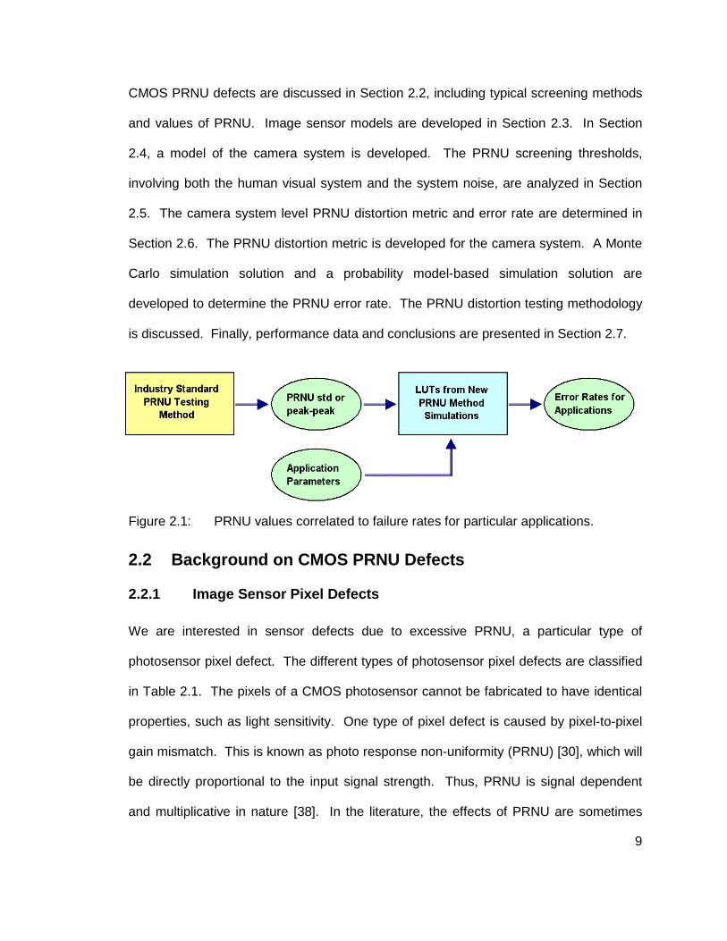
2.1 PRNU values correlated to failure rates for particular applications. 9

2.2 Pixel to pixel variations of photodiode and source follower transistor. 11

2.3 Pixel to pixel gain pdf, normalized by mean value. Characterization data from Conexant 20490 DVGA sensor. The X parameter is the standard deviation of the normalized pixel gain distribution (σPixel_Gain=σgain/µgain), which varies from sensor to sensor. 14

2.4 Expected PRNU metric values as a function of PRNUrms, the standard deviation of the normalized pixel gain distribution (σgain/µgain), for Conexant DVGA resolution sensor, 4µm x 4µm pixel, with 5084 8x8 blocks. ‘max’ is maximum value from all of the 5048 blocks. The mean block PRNUP-P is appox. 4.5% when the mean block PRNUrms is 1%. The expected maximum PRNU values are 6.7% for PRNUP-P and 1.4% PRNUrms when PRNUrms is 1%. For sensors with PRNUrms=1.5%, we expect the mean PRNUP-P to be 6.8%. For a DVGA resolution sensor, this corresponds to a maximum PRNUP-P value of 10% (and max PRNUrms of 2%), which is a commonly used value for the testing PRNU threshold. 17

2.5 PRNU peak to peak and rms values for two different pixel PRNU distributions. The left block has a Gaussian PRNU distribution (PRNUP-

P=4%, PRNUrms=0.87%). The right block has impulse noise for two outliers, with the remainder of the pixels having no PRNU (PRNUP-P=10%, PRNUrms=0.87%). The contrast has been exaggerated to enhance PRNU visibility. 19

2.6 Distributions for the two 8x8 blocks shown in Figure 2.5 (left block has a Gaussian-like PRNU distribution, right block has impulse). 20

2.7 Noise transfer diagram. 21

ix

2.8 Noise versus sensor output for noise sources. DVGA sensor operated at base gain setting (1x). Simulation results based upon measurement values of conversion gain, read noise, dark current noise, and full well for a CMOS sensor [17]. Noise model is constructed using these parameter values. 27

2.9 Noise versus sensor output for noise sources. DVGA sensor operated at gain setting 4x. Simulation results based upon measurement values of conversion gain, read noise, dark current noise, and full well for a CMOS sensor [17]. Noise model is constructed using these parameter values. 28

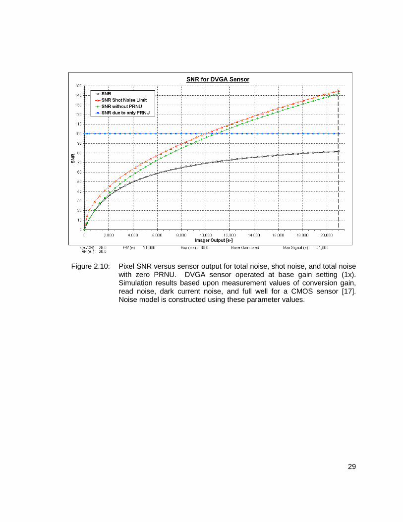
2.10 Pixel SNR versus sensor output for total noise, shot noise, and total noise with zero PRNU. DVGA sensor operated at base gain setting (1x). Simulation results based upon measurement values of conversion gain, read noise, dark current noise, and full well for a CMOS sensor [17]. Noise model is constructed using these parameter values. 29

2.11 Total noise versus PRNU noise factor. DVGA sensor operated at base gain setting (1x). Knee locations indicate that non-PRNU noise and PRNU noise are of equal magnitude. Simulation results based upon measurement values of conversion gain, read noise, dark current noise, and full well for a CMOS sensor [17]. Noise model is constructed using these parameter values. 30

2.12 Photon Transfer Curve for a DVGA sensor operated at base gain setting. Simulation results based upon measurement values of conversion gain, read noise, dark current noise, and full well for a CMOS sensor [17]. Noise model is constructed using these parameter values. 31

2.13 System level error tolerance model. 35

2.14 Relationship of distortions D1 and D2, along with W, WN and WN+P and their quantized values. Photon shot noise and read noise combined with quantization distorts the input signal value W to Q(WN). The addition of the noise sources, including PRNU, combined with quantization distorts the input signal value W to Q(WN+P). We are interested in the increase in distortion, from D1 to D2, due to PRNU. 46

2.15 Example showing relationship of quantized signals and quantization bin size. The upper portion of the figure shows a smaller quantization bin size that results in Q(WN) and Q(WN+P) being in different bins, while the lower portion shows the two quantized signals being in the same bin for a larger bin size. We see how the noise terms (PRNU and non-PRNU noise) affect the quantization of the input image data W. As the bin size shrinks, the corrupted signal WN+P enters the adjacent bin. 50

x

2.16 Example showing how distortion metric DC3 can be a poor metric for

measuring PRNU distortion. Here, DC3 has a large value, however, the

distortion with and without PRNU is the same (DC1=DC

2). We also see that PRNU and non-PRNU noise can have opposite signs. 51

2.17 Case 1b, with DC2<∆Q, PRNU forces quantized signal to next bin, but

distortion is less than quantization step size. 53

2.18 Case 1b, with DC2>∆Q, PRNU forces quantized signal to next bin, and

distortion is equal to quantization step size. 53

2.19 Case 2a, DC2 = DC

1 , PRNU has no effect on quantized signal. 54

2.20 Case 2b, DC2 = DC

1 + ∆Q , PRNU forces quantized signal to next bin. 54

2.21 Depiction of the pixel error components: L∆ and e’. 59

2.22 Relationship between distortion, ∆D, and clean input image signal value, W, for Case 1b, with DC

2<∆Q, L=0. The region of the input signal values where the threshold is exceeded (∆D>Th) is defined by Bi. 63

2.23 Relationship between distortion, ∆D, and clean input image signal value, W, for Case 1b, with DC

2>∆Q and e’N<∆Q/2, L=0. The region of the input signal values where the threshold is exceeded (∆D>Th) is defined by Bi. 65

2.24 Relationship between distortion, ∆D, and clean input image signal value, W, for Case 1b, with DC

2>∆Q and e’N>∆Q/2, L=0. The region of the input signal values where the threshold is exceeded (∆D>Th) is defined by Bi. 68

2.25 Relationship between distortion, ∆D, and clean input image signal value, W, for Case 2b, with DC

2>∆Q and 0<Th≤∆Q, L=0. 69

2.26 Analysis path (Flow Diagram) of proposed PRNU Monte Carlo distortion screening method. 80

2.27 Monte Carlo and probability model-based simulation PRNU failure rate method curves for variable sensor gain at the base DCT quantization setting. Conventional PRNU failure rate curve is also shown. The ‘knee’ point is close to the mean block PRNUrms (σgain/µgain) value of 1.5, which corresponds to a maximum block PRNUP-P value (limit) of 10% for a sensor with approximately 300K to 1M pixels. ‘Quant Factor=1’ signifies that the DCT quantization matrices of Table 2.6 were applied. 81

xi

2.28 PRNU failure rate curves for sensor gain setting of e-/DN=28 (base gain) and variable with variable DCT quantization applied. ‘Quant Factor’ is the multiplicative terms applied to the JPEG DCT quantization matrices shown in Table 2.6. The far left curve is the case where DCT quantization was not applied and the lowest gain setting was used. This case is severe, and is not typically used for determining PRNU failure. 82

2.29 Sample image used or Monte Carlo PRNU screening method and to generate probability data for the probability model-based simulation method. 83

3.1 Photonic and electronic forms of pixel cross-talk. 87

3.2 Bayer CFA pattern (typical types: red, green even, green odd, blue). 88

3.3 Cross-talk loss coefficients for a typical small pixel CMOS sensor [17]. 88

3.4 Simple blurring and additive noise problem. 93

3.5 Calculations of the color correction matrix for a typical low-cost camera sensor. 102

3.6 Typical low-cost camera color correction matrix adjustment. 103

3.7 HVS is sensitive to low spatial frequency color saturation [64], [85] and their errors. 108

3.8 Local extent of the cross-talk blurring and correction filters. Each blurring and correction will consist of between 4 and 9 pixels. 113

3.9 Regularization matrix equation showing the relationship between the corrected CCC ji term at pixel k, and the observed channel j pixel values in the local neighborhood of pixel k. Local pixel k component ji shown calculated for local extent regularization, where Nf will usually be between 4 and 9. 120

3.10 Restoration dB SNR improvement performance and complexity comparisons. Performances averaged over operating mean pixel SNR range of input 10 to 40. Improvement measured relative to uncorrected data. ST and CLS iterative restorations are non-spatially adaptive. 140

3.11 Corrected dB SNR improvements as a function of input image SNR. SNR values are mean of all of the image pixels. 142

3.12 CCC j to i βji terms (blue to green odd) as a function of local pixel SNR, with the maximum corrected SNR values per input SNR normalized to unity. Off-diagonal blurring CCC filters often are ill-conditioned, requiring larger optimal βji terms. The optimal βji value becomes large (>5) when the input mean pixel SNR value becomes small (<10). 144

xii

3.13 3-D surface plot of CCC j to i βji terms (blue to green odd) as a function of local mean pixel SNR, with the maximum corrected SNR values per input SNR normalized to unity. The optimal βji value becomes large (>5) when the input mean pixel SNR value becomes small (<10). 145

3.14 CCC i to i βii terms (green odd to green odd) as a function of local pixel SNR, with the maximum corrected SNR values per input mean SNR normalized to unity. There is a dark red (maximum corrected SNR) region close to the left edge of the plot (at β<0.01). On-diagonal blurring filters are better conditioned, requiring smaller optimal βii terms. The optimal βii value remains small (<0.1) even when the input mean pixel SNR value is small (<10), and the optimal βii value is very small (<0.001) when the input SNR is in it's normal operating range (>10). 146

3.15 3-D surface plot of CCC i to i βii terms (green odd to green odd) as a function of local pixel SNR, with the maximum corrected SNR values per input SNR normalized to unity. The optimal βii value remains small (<0.1) even when the input mean pixel SNR value is small (<10), and the optimal βii value is very small (<0.001) when the input SNR is in it's normal operating range (>10). 147

3.16 Ideal input test image used for performance analysis. 148

3.17 Input test image detail section corrupted for conversion factor e-/DN=1.4, Overall SNR=30, 18% Gray SNR=18. Images with any specified SNR value can be constructed using characterization and camera system models. 149

3.18 Detail of SNR=30 image section after correction by methods: Top Left: Optimal 3x3 Matrix, Overall SNR=35, 18% Gray SNR=15, Top Right: Overall SNR=37, 18% Gray SNR=16, Bottom: SCLS SNR, Overall SNR=42, 18% Gray SNR=18. 150

4.1 DCT coefficients of non-interpolated raw Bayer pixel data. 159

4.2 Correction of Bayer data in the DCT domain, correction applied to each coefficient i within the 8x8 DCT block of color plane k. 159

A.1 CMOS imager noise transfer diagram. 174

A.2 Three transistor active pixel based on a photodiode element. 174

B.1 Photon transfer curve for CMOS sensor. K(e-/DN) is 31 at dark level and 36 at saturation level. Read noise is 25 e-, total noise in dark is 28 e-, full well is 21,000 e-. 178

xiii

C.1 Typical low-cost camera color correction processing path. 191

C.2 Calculations of the color correction matrix for a typical low-cost camera sensor. 192

C.3 Typical low-cost camera color correction matrix adjustment. 193

xiv

Abstract

Image sensor testing and image quality enhancement methods that are geared towards

commercial CMOS image sensors are developed in this thesis. The methods utilize

sensor characterization data and camera system image processing information in order

to improve their performance.

Photo Response Non-Uniformity

An image sensor system-level pixel-to-pixel photo-response non-uniformity (PRNU) error

tolerance method is presented in Chapter 2. A novel scheme is developed to determine

sensor PRNU acceptability and corresponding sensor application categorization.

Excessive variation in the sensitivity of pixels is a significant cause of the screening

rejection for low-cost CMOS image sensors. The proposed testing methods use the

concept of acceptable degradation applied to the camera system processed and

decoded images. The analysis techniques developed give an estimation of the impact of

the sensor’s PRNU on image quality. This provides the ability to classify the sensors for

different applications based upon their PRNU distortion and error rates.

Perceptual criteria are used in the determination of acceptable sensor PRNU limits.

These PRNU thresholds are a function of the camera system’s image processing and

sensor noise sources. We use a Monte Carlo simulation solution and a probability

model-based simulation solution along with the sensor models to determine PRNU error

xv

rates and significances for a range of sensor operating conditions. We develop

correlations between conventional industry PRNU measurements and final processed

and decoded image quality thresholds. The results show that the proposed PRNU

testing method can reduce the rejection rate of CMOS sensors.

Cross-Talk Correction

A simple multi-channel imager restoration method utilizing a priori sensor

characterization information is presented in Chapter 3. A novel method is developed to

correct the channel dependent cross-talk of a Bayer color filter array sensor with signal-

dependent additive noise. We develop separate cost functions (weakened optimization)

for each color channel component-to-color channel component. Regularization is

applied to each color channel component-to-color channel component, instead of the

standard per color channel basis (giving us four optimal regularization parameters per

color channel). This separation of color components allows us to calculate regularization

parameters that take advantage of the differing magnitudes of each color channel

component-to-color channel component cross-talk blurring, resulting in an improved

trade-off between inverse filtering and noise smoothing.

The restoration solution has its regularization parameters determined by maximizing the

developed local pixel SNR estimations. The restoration method is developed with the

goal of viable implementation into the on-chip digital logic of a low-cost CMOS sensor.

The separate color channel component-to-color channel component approach simplifies

the problem by allowing a set of four independent color channel component

optimizations per pixel. Local pixel adaptivity can also be easily applied. Performance

data of the proposed correction method is presented using color images captured from

low cost embedded imaging CMOS sensors.

1

Chapter 1

Introduction

Trends in embedded imaging show that CMOS image sensors will continue to be

reduced in size and have an increased number of smaller pixels [33]. This causes the

delivery of sensors that produce good quality images to be more challenging. For

CMOS image sensors, more digital functionality and self-calibration will continue to be

integrated into the sensors in order to cope with image quality issues. It is very

important to have accurate and meaningful testing of these sensors, as the yield rate

directly affects profitability. The main idea developed in this thesis is the use of the

performance characteristics of CMOS image sensors and their camera systems to guide

and optimize the screening of the sensors and the processing of the sensor image data.

A testing method is developed in Chapter 2 to determine sensor pixel-to-pixel photo-

response non-uniformity (PRNU) acceptability and corresponding sensor application

categorization. In Chapter 3, a restoration method that can be implemented in on-chip

logic is developed to correct the color channel dependent cross-talk of a Bayer color

filter array sensor. Detailed information on CMOS image sensor characterization

required to develop these image quality testing and optimization approaches is

presented in the Appendices.

2

1.1 Pixel Response Non-Uniformity

Normally when sensor PRNU testing is performed, the temporal noise is removed by

multiple frame averaging [8], [17]. When this is done, most of the photon shot noise,

read noise, dark current shot noise, and other temporal noise sources are eliminated.

Only fixed pattern noise due to pixel offset (mean dark current, pixel voltage offset)

variation and pixel gain variation (PRNU) remain. The pixel offset variation can be

removed by black frame subtraction. The standard testing method does not consider

that the visibility of the PRNU can be reduced or hidden by these temporal noise

sources. The effects of the image processing performed (color correction, cross-talk

correction, etc.) along with the JPEG quantization on the visibility of PRNU are also not

considered. In practice, a heuristic PRNU threshold is frequently determined by finding

a visually acceptable level of PRNU for a worst-case operational condition [17]. Many

different factors will determine the image processing that will be performed, such as

designed camera application, transmission characteristics of the pixel color filters and

the infra-red filter, and so forth. The approach taken in Chapter 2 is to consider the

complete camera system, including its operating conditions (light levels, exposure times,

ISO number, image compression requirements, etc.), when evaluating acceptable PRNU

levels. Acceptable distortion values due to PRNU are determined based on camera

system characterization parameters and human visual system sensitivities to errors in

the DCT space.

Once these acceptable PRNU levels are determined for a particular sensor design for

use in a particular application, we can screen individual sensors for PRNU using

standard industry methods with the derived thresholds. The PRNU thresholds can be

determined for multiple applications. Thus sensors that fail PRNU screening for one

3

application, may be shown to acceptable for use in another application. For example, for

many consumer applications, low-light performance and color accuracy are important.

For industrial applications, frame rate may be more important. Different applications

may be concerned with different aspects of the pixel’s performance, such as sensitivity,

dynamic range, or noise [33].

Different sensors will have different signal to noise behavior, composed of differing

relative amounts of read, shot, and PRNU noise. Additionally, the different applications

will call for the sensor to be operated in different manners (exposure times, gain

settings) with different amounts of compression (controlled by desired data rates).

Further, each camera system will have different image processing, including color

processing tied to specific color filter arrays, and so forth. All of these factors will result

in a complex system, with many different parameters, which will affect the allowable

PRNU of the sensor. For this reason, it is advantageous to have sensor and camera

system models that can be run through a set of defined analyses which can determine

PRNU screening values that can be applied in simple standard sensor tests. Two

different sensor PRNU testing methodologies are developed in this thesis: a Monte Carlo

simulation solution and a probability model-based simulation solution. Both of these

methodologies allow for the screening of sensors for different applications.

1.2 Bayer Cross-Talk Problem

In Chapter 3, we derive a multi-channel, Bayer color filter array (CFA), adaptive pixel-

wise, direct regularized correction solution that optimizes the local low-frequency

component signal-to-noise ratio (SNR) of each corrected pixel. Our solution is geared

towards application in a simple, low cost camera system (e.g., camera phone). This

4

application requirement results in a trade-off between accuracy of the solution and

algorithm complexity (affecting the ability to implement the solution) [5]. In order to

accomplish our restoration goal, we develop a method to estimate the local mean SNR

value of the reconstructed local pixel signal using a deterministic reconstruction

approach (developed in section 3.3). The use of local estimations avoids an indirect,

iterative process. A method is derived to estimate the constrained least-squares (CLS)

regularization reconstructed bias and variance errors. In order to have a simple, closed

form solution, the multi-channel problem is reduced to a set of independent color

channel component to color channel component equations (developed in section 3.3.1).

An important property of the separation of color channel components is that it allows the

separate optimization of each color channel component. This results in each color

channel component being corrected based on the ill-conditioned-ness (stability) of its

blurring filters and its local signal to noise ratio. Since within color channel components

are typically more stable, their correction will be closer to the ideal, non-regularized

solution than that of the cross color channel components, which are less stable. This is

an improvement over existing multi-channel restoration methods, which usually use a

single regularization parameter per color channel (not per color channel component)

[27], [44]. Separating the color channel component also allows the optimal

regularization parameters for each color channel component to be solved offline and

used to create look up tables for pre-calculated parameters as a function of local SNR

values. Complete sets of convolution filter coefficients as a function of color channel

local SNR values can also be stored. This permits a simple, real time application of the

restoration.

5

Determining the regularization parameters using the local pixel SNR of each color

channel component, instead of using MSE, noise and signal energy bounding, or other

criteria, improves our correction by adhering to the sensitivity of HVS to the local SNR

and low-frequency color error [7], [56], [64], [73], [75], [76]. Local pixel SNR optimization

combined with the separation of color channel components, and the typically greater

stability of the with-in channel cross-talk blurring filters, results in the presented

restoration method giving priority to color white balance for all camera-operating

conditions. However, the amount of color saturation correction (cross-channel de-

blurring) will be dependent upon the sensor SNR levels. This behavior is consistent with

the heuristic methods used in low-cost camera systems, but it will be more adaptive both

spatially and dynamically.

1.3 Contributions of the Research

In this thesis, we present novel image sensor testing and correction methods which are

applied to CMOS imagers. These algorithms use sensor characterization information,

and are designed to be implementable in commercial, real-world applications. These

methods utilize original approaches, as outlined in the following subsections.

1.3.1 Contributions of Pixel Response Non-Uniformity Testing Method

We have developed a novel CMOS imager PRNU testing method which uses

information from the complete camera system. The key novelties in our approach are:

• Our PRNU testing method is innovative in using the concept of

acceptable degradation applied to the complete camera system. The

developed analysis techniques give an estimation of the impact of the

sensor’s PRNU on image quality. The human perceptual criteria are used

in the determination of acceptable sensor PRNU limits. Our solution

6

determines the effect of the complex camera system, with many different

parameters, on the allowable PRNU of the sensor. This is a unique

application of the concept of error tolerance. Sensor operating

conditions, sensor noise performance, image processing and

compression are all considered in the threshold and rate determinations.

Typically, fixed heuristic or empirical PRNU thresholds are used in

testing.

• Our solution allows for the industry standard testing method to still be

used. Using our modeled thresholds for multiple sensor applications, one

test can be used to categorize each sensor for one or more of a set of

possible sensor applications. This provides the ability to classify the

sensors for different applications based upon their PRNU distortion and

error rates. Thus, we allow for simultaneous testing for a set of sensor

applications. Typically, sensor retesting would be performed for each

sensor application.

1.3.2 Contributions of Bayer Cross-Talk Solution

We proposed a new solution for the Bayer CMOS imager cross-talk problem which is

simple, non-iterative, non-recursive and can be implemented in the on-chip digital logic

of an imaging sensor. The scheme takes into account the requirements and constraints

of a typical low-cost commercial embedded camera system. Our solution is unique in

combining the following method approaches and features:

• We separate each color channel into a sum of color channel components

and apply a separate regularization of each color channel component.

We refer to this as our separate color channel component constrained

least squares (SCLS) regularization. Regularization is usually done per

image or color channel [27], [44], [62]. The color channel component

regularization approach is novel. We exploit the differing degrees of color

channel component blurring filter ill-condition-ness and take advantage of

7

differing color component filter stabilities. The variation of local color

channel component SNR is also exploited. We also use color channel

component separation to simplify calculations, which allows for a practical

camera system implementation.

• We utilize a priori sensor data obtained from characterization. This

results in a coupling of the image sensor and the correction algorithms.

Simple signal magnitude dependent noise models obtained from sensor

characterization are used to define pixel SNR behavior. We obtain

stationary blurring models and independent Gaussian noise models.

Direction-dependent, asymmetrical and wavelength dependent cross-talk

models are also used to create pixel neighborhood directional filters.

• We address the human visual system (HVS) sensitivities in the solution,

including the sensitivity to local signal to noise contrast (SNR) and low

spatial frequency color accuracy sensitivity [7], [56], [64], [73], [75], [76].

Our developed solution also conforms to industry standard testing

methods (e.g., ISO12232-1998E). Our use of SNR constraints results in

a simplification of the calculations, and makes the implementation in a

low-cost camera system possible.

• We use the local pixel SNR to calculate the regularization parameter. We

have not seen this approach proposed among the published correction

methods. Other solution metrics do not match HVS’s sensitivity to local

SNR and low-frequency color error [3], [26], [48]. Our solution is adaptive

to global operating conditions and local image SNR conditions. Spatially

adaptive corrections are used in our solution, which are coupled with the

color component separation. The correction method results in a pixel

scalar solution form. Additionally, using the local mean estimate for local

SNR values improves the accuracy of our estimate through noise

smoothing. The local mean value also matches the HVS’s color error and

SNR sensitivities.

8

Chapter 2

Photo-Response Non-Uniformity Error Testing

Methodology for CMOS Imager Systems

2.1 Introduction

In this chapter, we develop methods to determine acceptable pixel response non-

uniformity (PRNU) levels which take into account the complete camera system. We

evaluate the effect of image sensor PRNU defects at the output of the camera system.

Camera system characterization parameters and human visual system sensitivities to

errors are used to find acceptable PRNU distortion values. These calculations are done

off-line for a particular sensor and camera design, allowing the standard industry PRNU

testing to still be used. Our general approach of correlating conventional testing method

PRNU measurements to a set of application specific error rates is shown in Figure 2.1.

Conventional PRNU testing is used to measure PRNU error metrics for a set of sensors.

As shown in the figure, these measured PRNU errors are then used to determine the

error rates for each sensor for a set of different applications.

9

CMOS PRNU defects are discussed in Section 2.2, including typical screening methods

and values of PRNU. Image sensor models are developed in Section 2.3. In Section

2.4, a model of the camera system is developed. The PRNU screening thresholds,

involving both the human visual system and the system noise, are analyzed in Section

2.5. The camera system level PRNU distortion metric and error rate are determined in

Section 2.6. The PRNU distortion metric is developed for the camera system. A Monte

Carlo simulation solution and a probability model-based simulation solution are

developed to determine the PRNU error rate. The PRNU distortion testing methodology

is discussed. Finally, performance data and conclusions are presented in Section 2.7.

Figure 2.1: PRNU values correlated to failure rates for particular applications.

2.2 Background on CMOS PRNU Defects

2.2.1 Image Sensor Pixel Defects

We are interested in sensor defects due to excessive PRNU, a particular type of

photosensor pixel defect. The different types of photosensor pixel defects are classified

in Table 2.1. The pixels of a CMOS photosensor cannot be fabricated to have identical

properties, such as light sensitivity. One type of pixel defect is caused by pixel-to-pixel

gain mismatch. This is known as photo response non-uniformity (PRNU) [30], which will

be directly proportional to the input signal strength. Thus, PRNU is signal dependent

and multiplicative in nature [38]. In the literature, the effects of PRNU are sometimes

10

considered to be one component of fixed pattern noise (FPN) [9]. However, in this

thesis, we use the more common definition which considers FPN to consist of signal-

independent time-invariant noise, while PRNU is considered as a signal-dependent time-

invariant noise [11], [20].

Table 2.1: Pixel defect types.

Pixel Defect Type Cause

Hot Pixel Fabrication imperfection:

Pixel stuck high

Cold Pixel Fabrication imperfection:

Dead pixel, pixel stuck low

PRNU Fabrication imperfections,

Poor pixel design:

Photodiode size variation

Photodiode capacitance variation

Source follower transistor gain variation

Coating variation

High Dark Current Fabrication imperfection:

Pixel dark current variation

2.2.1.1 Causes of PRNU

The photodiode area of pixels in CCD and CMOS sensors can vary, resulting in variable

gain from pixel-to-pixel. The main causes of variable pixel gain are photodiode

capacitance variation and deviations in the surface area of the photodiodes [42]. The

pixel conversion gain is proportional to the inverse of the photodiode capacitance (pixel

gain ∝ q/C). Photodiode capacitance deviations are due to variations in the properties of

the substrate and diode material (manufacturing doping issues). Variations in

11

photodiode surface area lead to differences in the number of photons being captured by

a pixel. Another cause of pixel gain differences is the deviation in the thickness of color

filter array (CFA) coatings, which result in different pixel photon transmission values.

Pixel gain variations of 1 to 5 percent (rms) are common [39]. For APS CMOS pixels,

the source-follower transistors can have variations in both gain and offset. Variations in

pixel gain are complicated and expensive to correct in a camera system. For low cost

camera systems, pixel gain variation is usually not corrected. The PRNU defective

pixels are usually randomly distributed across the sensor array. These defects are

depicted in the pixel schematic shown in Figure 2.2.

Figure 2.2: Pixel to pixel variations of photodiode and source follower transistor.

One of the major disadvantages of CMOS sensors compared to CCD sensors is the

lower yield of the former due to excessive PRNU [32]. CMOS sensors usually have

moderate or low pixel response uniformity [20]. However, CMOS sensors offer many

advantages over CCD sensors. CMOS sensors can be manufactured at a lower cost,

can integrate digital logic on the chip (e.g., ADC, JPEG logic, ‘camera-on-a-chip’),

consume less power, and be more compact in area (through integration of components

on chip) [51].

12

2.2.1.2 Hot and Cold Pixel Defects

Due to fabrication errors, as the number of pixels in a photosensor increases, the

likelihood of the sensor having stuck hot and cold pixels defective pixels is high. These

defects occur at pixels whose output values are either stuck high (Vdd) or low (Gnd).

Pixels with very high levels of PRNU can be interpreted as hot or cold pixels. Hot and

cold pixel defects can be corrected during camera operation using simple spatial filtering

algorithms [6], [81]. The shot noise time variation of dark current appears as temporal

noise. Pixels with extremely high dark current (refer to Appendix A) are often treated as

hot pixel defects.

2.2.2 Reasons for Studying PRNU Defect Testing

We will consider only PRNU defects in this analysis. The reasons for this decision are:

1) Hot and cold pixels are usually identified during wafer or device testing

and are marked for correction (pixel value replacement) using

neighboring pixel values. In contrast, PRNU defective pixels are usually

not corrected by the imaging system, unless the PRNU values are so high

as to appear as a hot or cold pixel.

2) Variation in the pixel response is unavoidable. Pixels with PRNU values

which exceed standard testing thresholds, and are thus rejected, are

often more likely to occur than hot or cold pixels. As discussed,

excessive PRNU is a major cause of yield loss for CMOS sensors [32].

3) Image sensors that have large numbers of hot or cold pixels (especially

clusters of these pixels) are usually regarded as unusable, and cannot be

salvaged.

For these reasons, we wish to study the PRNU defect in order to improve photosensor

yield through increasing the acceptable defect rate and allowable threshold. We will also

13

be able to classify sensors for particular applications based on the developed PRNU

screening method. PRNU is a problem with a continuous range of characteristics, i.e.,

differing degrees of response non-uniformity. Our goal is to increase the fault tolerance

for this type of pixel defect by considering the complete image processing chain, full

sensor noise model, and sensor application operating parameters.

2.2.3 PRNU Characterization

Sensor characterization data is used to create a typical probability density function (pdf)

for a CMOS sensor’s pixel gain. In Figure 2.3, we show the local area pixel gain

variation (pdf) for a CMOS sensor obtained from a typical sensor lot [17], [18]. The data

was generated using a large set of pixel gain measurements. The measurements were

taken over local pixel areas (in this case 8x8 pixel areas). The pixel gain plot has been

normalized using the mean pixel gain (µgain) to give a mean gain of unity. The results

shown are the mean distribution values of the collected local pixel areas. The parameter

X shown in the plot on the X-axis is the standard deviation of the normalized pixel gain

distribution (σPixel_Gain=σgain/µgain=PRNUrms). For a particular sensor design, the standard

deviation of the pixel gain distribution will vary from sensor to sensor. This change in

gain distribution is due to pixel design and manufacturing process (or wafer lot to lot

variation), as discussed previously. For a particular sensor design, the shape of the

distribution has been found to stay the same, with only the variance or gain variation

parameter changing from chip to chip [17]. Thus, one can obtain through sensor

characterization the basic shape and values of the PRNU distribution. Then the

distribution can be scaled to represent different magnitudes of PRNU. For what might

be considered good quality low-cost consumer sensors, the value of the standard

deviation of the pixel gain distribution has been found to be around 1%. This is the value

14

of σgain/µgain (PRNUrms) for the sensor family characterized in Figure 2.3 [18]. This

PRNUrms value is a fairly typical value for CMOS sensors [40]. The upper range of the

value of the gain variation parameter for some of the sensors within this design (and

other design families) may extend to 4.0 or more (σgain/µgain > 4).

Figure 2.3: Pixel to pixel gain pdf, normalized by mean value. Characterization data from Conexant 20490 DVGA sensor. The X parameter is the standard deviation of the normalized pixel gain distribution (σPixel_Gain=σgain/µgain), which varies from sensor to sensor.

2.2.4 Industry Standard PRNU Screening

The industry standard PRNU screening method is typically applied to monochrome

sensors still on the wafer (prior to dicing) and before the color filter array has been

deposited [17]. The PRNU screening is sometimes done after device packaging, with

each color tested separately. PRNU can be segmented into local PRNU and global

15

PRNU [10]. We will concentrate on local PRNU, since it causes the greatest failure

rates [9], [17]. Also, local measurement of PRNU matches well with the HVS’s

sensitivity to defects correlated within a small spatial area [7], [19], [73]. The HVS is less

sensitive to global variation of pixel gain (brightness). The standard screening method

consists of dividing the sensor’s image area into non-overlapping segments, often of size

8x8 or 10x10 pixels, under a normal exposure time condition [8], [17], [52]. Typically, the

response level of the pixels is set to be from 50% to 75% of full range [11] by applying

uniform illumination. PRNU is linear with signal, so we wish to create large values to

measure. PRNU is usually quantified in terms of the peak-to-peak pixel value divided by

the mean value (µgain) for each block (PRNUP-P) [17], [18]. Another popular metric is an

rms pixel value (σgain) divided by the mean value (µgain) for each block (PRNUrms). The

block with the largest value is often taken as the PRNU value for the chip, instead of

using a mean chip value. We will use the peak-to-peak method (PRNUP-P), as it seems

to be more commonly used. The peak-to-peak PRNU test is also considered better, as it

finds worst case pixels that will stand-out to the observer, whereas the PRNU rms test

can smooth-out one or more pixels within a block that are outliers. The peak-to-peak

PRNU test is also generally faster to calculate on a wafer or chip tester.

For both the peak-to-peak and rms PRNU measurement methods, temporal noise is

removed to leave only fixed pattern noise (FPN) [17]. This is done through multiple

frame averaging, where 16 or more frames may be used in the mean frame calculation.

When the FPN dark level offset is removed, we are left with essentially the PRNU.

Testing of the pixels can be done in the analog domain, by having the voltage values of

the pixels output. Often this is done by utilizing a test mode on the chip to by-pass the

on-chip ADC and output voltage levels to a pin, usually when the chips are still on the

16

wafer [17]. For each segment (e.g., 8x8 or 10x10 area of the sensor), the average

analog output voltage (Vout) is found for the mean frame. The maximum and minimum

pixel voltage values of each segment’s mean frame are also calculated, given by Vmax

and Vmin, respectively. The peak-to-peak PRNU is then defined as:

PRNUP-P = (Vmax – Vmin) / Vout (2.1)

We can also perform this operation in the digital domain using digitized pixel values from

the on-chip ADC. This is often done on the chip level, after the wafer has been diced.

The sensor can be in the camera system, or simply in its package. When performed in

the digital domain, the methodology will be the same. The only difference is that the

variables Vmax, Vmin, and Vout will be digital numbers read directly from the sensor

output, instead of voltage levels. During this testing, the pixels previously identified as

being hot or cold pixels should not be used in the calculations. The assumption made is

that these pixels will be corrected, usually using values taken from their neighbors.

Sensors that have too many hot or cold pixels will have been rejected prior to the PRNU

screening test.

The measured PRNU value is compared with a threshold value. The PRNU threshold

value used will often be determined for a particular type of camera application.

Consumer applications have PRNU peak-to-peak thresholds that vary from 10% for mid

to low-end applications [16] to 5% for more stringent applications. The PRNU block

error rate will be equal to the number of blocks that fail the PRNU test divided by the

total number of pixel blocks on the sensor array. Using data from many sensors, it

represents the probability that a sensor will have a block that fails the PRNU test. Some

17

applications may call for zero defective PRNU blocks, while others allow for one or more

blocks failing.

2.2.5 PRNU Screening Metric Behavior

In Figure 2.4, we show expected PRNU metric values as a function of the standard

deviation of the normalized pixel gain distribution (σgain/µgain=PRNUrms) for the sensor

with the pixel gain distribution shown in Figure 2.3.

Figure 2.4: Expected PRNU metric values as a function of PRNUrms, the standard deviation of the normalized pixel gain distribution (σgain/µgain), for Conexant DVGA resolution sensor, 4µm x 4µm pixel, with 5084 8x8 blocks. ‘max’ is maximum value from all of the 5048 blocks. The mean block PRNUP-P is appox. 4.5% when the mean block PRNUrms is 1%. The expected maximum PRNU values are 6.7% for PRNUP-P and 1.4% PRNUrms when PRNUrms is 1%. For sensors with PRNUrms=1.5%, we expect the mean PRNUP-P to be 6.8%. For a DVGA resolution sensor, this corresponds to a maximum PRNUP-P value of 10% (and max PRNUrms of 2%), which is a commonly used value for the testing PRNU threshold.

18

The data was generated using measured pixel gain pdfs from a set of sensors. The

pixel gain pdfs were scaled in order to get a realistic range of sensor PRNU

performance. This scaling was applied to the standard deviation value of the pixel gain

pdf. The sensor pixel data was then used to calculate the different PRNU metric values.

The plot shows the anticipated linear relationship between different PRNU metrics and

the standard deviation of the normalized pixel gain distribution (σgain/µgain). The expected

maximum PRNU values for a sensor will be a function of the number of pixel blocks that

make up the array. As the size of the sensor array increases, the probability of at least

one pixel block failing the PRNU test increases. For a sensor with this pixel gain

distribution and many 8x8 blocks, there can be a fairly high probability of the sensor

having at least one defective PRNU block. Many commercial imager designs have less

than a 1% sensor rejection rate due to PRNU [15]. However, yield losses of up to 4.5%

have been seen in CMOS image sensor manufacturing [17].

Finally, we discuss the advantage of using a peak-to-peak metric for measuring PRNU

instead of a rms metric. In Figure 2.5 we show two different sensor block PRNU

responses. The distributions of the pixel responses are shown in the histograms of

Figure 2.6. One of the 8x8 pixel blocks has a Gaussian pixel gain distribution, while the

other one has uniform pixel gain with two impulse-like pixel gain outliers. The measured

mean, standard deviation, and PRNUrms of each block are all the same. However, the

PRNUP-P value of the image on the right is much greater. This is due to the image on

the right having a zero PRNU value for all pixels except for two pixels that are extreme

outliers. Since the image on the left has a Gaussian distribution of PRNU, its greatest

PRNU outliers are not as extreme as the image on the right. Due to the HVS’s

sensitivity to brightness contrast [7], the PRNU of the image on the right is more visible.

19

If we were to use the PRNUrms metric, we would not have been able to distinguish

between these two relatively low and high PRNU visibility cases (left and right images,

respectively). Thus, we can see that the PRNUP-P method of calculating a PRNU metric

is more in-line with the way the HVS functions. Our developed PRNU screening metric

must be sensitive to peak-to-peak differences within blocks As we shall see in Section

2.5 when we develop our distortion metric, we will use a ‘Peak Contrast’ model of

Minkowski pooling, as opposed to linear summation. This approach adheres to the

conventional PRNUP-P testing method of looking at pixel PRNU outliers.

Figure 2.5: PRNU peak to peak and rms values for two different pixel PRNU distributions. The left block has a Gaussian PRNU distribution (PRNUP-

P=4%, PRNUrms=0.87%). The right block has impulse noise for two outliers, with the remainder of the pixels having no PRNU (PRNUP-P=10%, PRNUrms=0.87%). The contrast has been exaggerated to enhance PRNU visibility.

20

Figure 2.6: Distributions for the two 8x8 blocks shown in Figure 2.5 (left block has a Gaussian-like PRNU distribution, right block has impulse).

2.2.6 Typical Sensor Values of PRNU

We have seen that the performance of CMOS sensors is traditionally often limited by

PRNU [9]. PRNU measurement values are reported in Table 2.2 for numerous sensors.

Table 2.2: Typical PRNU measurements for CMOS sensors.

Sensor Ref PRNU Sensor Information

[1] 2% rms High performance VGA resolution sensor

[21] 5% rms Commercial CMOS sensor

[51] 1.9% rms APS CMOS sensor, 0.35 µm technology

[51] 6.5% rms APS CMOS sensor, 0.18 µm technology

[69] 1% peak-to-peak Very large pixel size of 11.6 µm by 11.6 µm and low resolution. Pixel is impractical for mobile imaging.

In sensor documentations, PRNU rms values for CMOS sensors in the range of 1 to 5%

have been measured [39]. In making the rms measurements, the pixel mean response

is removed (unbiased estimator), giving the standard deviation, which is normalized

21

using the mean response (µ/σ). PRNU usually increases as the pixel size is decreased.

The particular CMOS technology used also affects PRNU. In cell phone applications,

pixel sizes are usually less than 3 µm by 3 µm [33].

2.3 Pixel Noise and Defect Characterization and Mod eling

2.3.1 Image Sensor Noise Model

In this section, we will develop noise models for our CMOS image sensors. We will

define a simplified camera system noise model that can be used in creating acceptable

threshold values for image distortion (see Section 2.5). As we will discuss later, the

presence of other noise sources can mask the effects of PRNU noise. Detailed

information on CMOS image sensor noise is presented in Appendix A.

CMOS image sensors experience noise from numerous noise sources. The resulting

noise has both time-invariant (fixed-pattern) and time-variant (temporal) behavior. The

use of the term fixed-pattern noise refers to any spatial pattern that does not change

significantly from frame to frame. In contrast, temporal noise changes from image frame

to frame. A noise transfer diagram is shown in Figure 2.7 for a typical CMOS imager

[35].

Figure 2.7: Noise transfer diagram.

22

The temporal (time variant) noise that CMOS sensors encounter includes [92]: photon

shot noise, capacitive reset (kTC) noise, dark current time-varying noise, Johnson

(thermal or white) noise, and 1/f noise (frequency-dependent). Additionally, CMOS

imagers can suffer temporal noise from electrical ground-bounce and coupling noise

problems generated by on-chip logic and ADC circuitry. Fixed pattern noise (FPN) is

generated in CMOS imagers by pixel variations in dark current and sensitivity, as well as

pixel fixed offset. It is common practice to express the values of the noise sources in

root mean square (RMS) electron values.

2.3.1.1 Noise Model Simplifications and Assumptions

For many camera systems, an adequate noise model can be constructed using only shot

noise, read noise, dark current noise (both fixed pattern and temporal), and PRNU noise

[35]. All of these noise sources can be considered to be uncorrelated from pixel-to-pixel

[35], [42]. Some of the noise sources are functions of the signal levels [35]. In the

development of our PRNU testing methodology, we will make the following commonly

used assumptions [35], [42]:

1) All individual noise sources are independent and thus their powers (variances)

can be added.

2) All noise components are white (in time and space for temporal noise, and in

space for fixed pattern noise).

3) Image processing operations applied to the sensor data will be limited to linear

functions.

4) A uniform image model [72] can be used to calculate the DCT-domain

quantization error, where it is assumed that the quantization step sizes are

reasonably small.

23

The assumption of linear image processing operations is a reasonable assumption for

most of the camera functions [43], such as Bayer interpolation, cross-talk correction,

color correction, color space conversion, and DCT transform (see Section 2.4). In order

to simplify our model and our noise estimations, we will restrict our image processing

modeling to only linear operations. Using the above simplifications, the total pixel noise

can be written as:

σpixel2 = σshot

2 + σread2 + σdark current

2 + σPRNU2 (2.2)

A noise model for a CMOS image sensor can be developed using characterization and

sensor performance theory. The model will be a function of the sensor operating

conditions, such as exposure time and input signal level.

When we incorporate the camera image processing, we will include quantization due to

the JPEG compression (not due to the analog-to-digital converter, ADC) into the pixel

noise equation. As listed above, we will use the simplifying assumption of a uniform

image model [72] to calculate the DCT-domain quantization error. We will also consider

noise amplification due to image processing operations. The effects of the image

processing will be taken care of in the camera system model (see Section 2.4).

2.3.2 Noise Models and Photon Transfer Curves

We now look at how the amount of PRNU affects the total noise of the sensor. This

relationship will help determine our visibility thresholds for PRNU, as shown in Section

2.5. As we have discussed, we can construct a simplified pixel noise model using

Equation (2.2) [35], [42]. In Figure 2.8 we show a typical base gain (lowest internal gain

setting of the sensor) noise plot. The sensor used for the noise model is a DVGA

24

resolution CMOS sensor with 3 transistor (3T) 4µm x 4µm APS pixel architecture. The

conversion gain (k) ratio of a sensor is defined as the amount of output generated (in

digital number values, DN) per unit charge (e-) created in the pixel [68], and has units of

e-/DN. This sensor has a base gain conversion factor of k=28 e-/DN, read noise of 28e-,

full well (usable pixel signal range) of 21,000 e-, pixel non-uniformity of 1.0% rms, dark

current rate of 1e-/ms, and was operated for a 30ms exposure time. These sensor

parameter values were taken from actual measurements of a CMOS sensor [17]. In the

plot, shot noise, read noise, dark current (FPN and TN), PRNU noise, and total noise are

shown. From the Figure 2.8, we can see that PRNU is the dominant noise source for

the majority of the pixel’s output signal range. When a sensor is operated at a higher

internal gain setting, the output range in the pixel in electrons is reduced. This can be

seen in Figure 2.9, where we show the noise plot for an internal gain setting of 4x (k=7

e-/DN). When the sensor is operated at this gain setting, the output signal range over

which the PRNU is the dominant noise source is reduced to the point that it is

eliminated. The upper output range of the pixel is now limited by the ADC, and is

clipped at the maximum output (7168 electrons in this case). The sensor would be set to

a larger gain when the amount of light reaching the sensor is lower (high ISO

conditions). This can occur for lower lighting conditions, shorter sensor exposure times,

or the use of higher f-number lens.

We show the signal-to-noise ratio (SNR) for the sensor in Figure 2.10. The SNR is

computed in the usual manner using mean output signal (e-) divided by total noise (e-).

We also show the situation when PRNU is removed from the total noise (gain variation

set to zero), when only signal shot noise is considered (shot noise limited case), and

when only PRNU noise is considered in the SNR calculation. Since PRNU noise is

25

proportional to signal, the SNR due to PRNU remains constant and independent of

sensor output magnitude. It is obvious from the plot that as the output signal

approaches the full well capacity of the pixel, the PRNU noise becomes the dominant

noise and limits SNR. The point of intersection of the total noise without PRNU SNR

curve with the only PRNU SNR curve shows the signal magnitude value when PRNU

begins to dominate. The signal value at which PRNU begins to dominate is

approximately 10,900 electrons.

In Figure 2.11 we show how variable amounts of PRNU affect the total noise of the

sensor. The plot shows that PRNU noise is not perceptible until the PRNU variable gain

percentage reaches an amount that causes a ‘knee’ in the total noise curve [35]. This

‘knee’ is defined to occur when the total noise without PRNU is equal to the PRNU

noise. This occurs when the total noise increases by a factor of 2 from its zero PRNU

value. We see from the plot that when the pixel is closer to full well, the perceptible

PRNU percentage threshold decreases. This is the same as saying that as the pixel

gain setting (user selected gain factor that is applied to the pixel data) is increased, the

perceptible PRNU percentage threshold increases.

The complete noise performance of an imaging sensor can be determined using the

photon transfer curve (PTC) technique [41]. The PTC method is discussed in greater

detail in Appendix B. In the method, the rms noise is plotted as a function of the signal

level, in unit of electrons. The method can be used to estimate the conversion gain (k)

of an imager [68]. The PTC method can be used to calculate a sensor’s read noise, full

well, linearity, dynamic range, and sensitivity [40]. A PTC is shown Figure 2.12 for our

test image sensor. At low input signal levels (low photon fluxes), the noise floor of the

26

sensor will dominate. This will determine the read noise. As the input signal increases,

the photon shot noise will increase. For most well-designed sensors, the sensor will be

‘shot noise limited’, i.e., the photon shot noise will be the dominant noise. As the charge

held by the pixel photodiode approaches saturation, the noise behavior can enter a third

region of behavior. This region is dominated by PRNU noise. Thus, the photon transfer

curve gives us the following important information: the level at which PRNU will be

visible, and the pixel region of operation when PRNU will not be a limiting factor on

sensor performance. Sensors can have values of PRNU low enough that the pixel will

not be dominated by PRNU noise. But in the case of low cost CMOS sensors, there is

usually a PRNU noise dominated noise region. As the input signal increases, the noise

will reach a maximum value and then abruptly drop [35]. This defines the saturation

point, where electrons will overflow from the pixel into neighboring pixels.

In the PTC, which is plotted on a log-log scale, a read noise region will have a noise-to-

signal slope close to zero, a shot noise limited region will have a slope of ½ (noise

variance equal to mean signal), and a PRNU limited region will have a slope of unity

(noise standard deviation proportional to mean signal). From the PTC shown in Figure

2.12, we can see the three noise regions. For low ISO sensor operation, which has

higher signal and SNR, typically pixels be operating in the PRNU region. This is due to

a greater range of the pixel’s response being exercised. For high ISO sensor operation,

which has lower signal and SNR, the PRNU will be less dominant. This is due to a lower

range of the pixel’s response being exercised. The upper response of the pixel (as it fills

up with electrons) will be clipped by the large gain applied (lower value of k).

In the full camera system analysis, we will use the image processing pipeline model as

well as the sensor noise model to determine the noise visibility threshold for PRNU. This

27

will be done in the DCT domain. Quantization noise from the JPEG compression

process will also be included in the system noise calculations. The noise values will be

a function of the DCT frequency components. The camera system model is presented in

Section 2.4.

Figure 2.8: Noise versus sensor output for noise sources. DVGA sensor operated at base gain setting (1x). Simulation results based upon measurement values of conversion gain, read noise, dark current noise, and full well for a CMOS sensor [17]. Noise model is constructed using these parameter values.

28

Figure 2.9: Noise versus sensor output for noise sources. DVGA sensor operated at gain setting 4x. Simulation results based upon measurement values of conversion gain, read noise, dark current noise, and full well for a CMOS sensor [17]. Noise model is constructed using these parameter values.

29

Figure 2.10: Pixel SNR versus sensor output for total noise, shot noise, and total noise with zero PRNU. DVGA sensor operated at base gain setting (1x). Simulation results based upon measurement values of conversion gain, read noise, dark current noise, and full well for a CMOS sensor [17]. Noise model is constructed using these parameter values.

30

Figure 2.11: Total noise versus PRNU noise factor. DVGA sensor operated at base gain setting (1x). Knee locations indicate that non-PRNU noise and PRNU noise are of equal magnitude. Simulation results based upon measurement values of conversion gain, read noise, dark current noise, and full well for a CMOS sensor [17]. Noise model is constructed using these parameter values.

31

Figure 2.12: Photon Transfer Curve for a DVGA sensor operated at base gain setting. Simulation results based upon measurement values of conversion gain, read noise, dark current noise, and full well for a CMOS sensor [17]. Noise model is constructed using these parameter values.

2.4 Imager System Model

We desire to analyze how input sensor PRNU error leads to final processed error in a

camera system after typical image processing of realistic image data (complete with

typical noise). We will seek to estimate the distortion between sensor systems that have

no PRNU noise and those that have varying degrees of PRNU. We propose to use

known or typical probability models for the input image (and noise) data, or alternatively

a Monte Carlo approach, where we use a set of images that will cover our input image

space. To accomplish this, we need to use an accurate camera system model, which

should include an accurate sensor noise model. A diagram used for the system level

error tolerance of a camera system is shown in Figure 2.13. The sensor pixels are

32

subject to noise, including photon shot noise, read noise (including dark current noise),

and PRNU. We will use the simplified, but realistic noise model that was developed in

Section 2.3. The diagram of Figure 2.13 includes the image-processing pipeline for a

typical low-cost consumer camera (including embedded imaging applications). The ideal

image input data F is first blurred by the camera optics of the system and subsampled by

the Bayer color filter array (CFA) pattern of the sensor, producing the image signal G.

Then signal magnitude dependent photon shot noise (ESN) is modeled as being added to

the signal when it reaches the pixel photodiode. Additional blurring of the image data

occurs due to signal exchange between local neighborhood pixels (cross-talk effects)

[60]. This multi-channel blurring is a multi-color signal convolution, which can be written

in the matrix multiplication form: Y° = HG°. . This pixel signal color cross-talk blurring effect

will have to be corrected as part of the color correction of the image processing, resulting

in some noise amplification [60]. Color cross-talk blurring is discussed in detail in

Section 3.1 and Appendix C. We then model the read noise (ERN) as being added to the

signal at this point, which produces the distorted image signal Gnoise. We define the read

noise as being the additive noise floor, which includes pixel reset noise, dark current

noise (temporal and fixed pattern), and so on.

The PRNU error is represented as the additive term EPRNU. Using our noise and signal

models, we can calculate the additive term EPRNU. The value of the multiplicative factor

used for the noise is taken from the probability density function of PRNU multiplicative

factors. The average PRNU distribution is taken from sensor characterization. Variation

in PRNU distributions is modeled as a multiplicative widening of the distribution, which

matches well with characterization data (refer to Section 2.3). After the addition of the

PRNU errors, the signal Gnoise+PRNU is scalar quantized by the on-chip ADC, producing

33

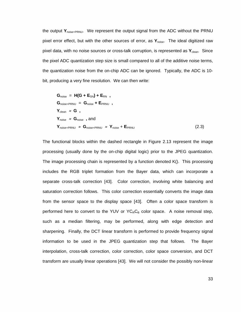
the output Ynoise+PRNU. We represent the output signal from the ADC without the PRNU

pixel error effect, but with the other sources of error, as Ynoise. The ideal digitized raw

pixel data, with no noise sources or cross-talk corruption, is represented as Yclean. Since

the pixel ADC quantization step size is small compared to all of the additive noise terms,

the quantization noise from the on-chip ADC can be ignored. Typically, the ADC is 10-

bit, producing a very fine resolution. We can then write:

Gnoise = H(G + ESN) + ERN ,

Gnoise+PRNU = Gnoise + EPRNU ,

Yclean ≈ G ,

Ynoise ≈ Gnoise , and

Ynoise+PRNU ≈ Gnoise+PRNU ≈ Ynoise + EPRNU (2.3)

The functional blocks within the dashed rectangle in Figure 2.13 represent the image

processing (usually done by the on-chip digital logic) prior to the JPEG quantization.

The image processing chain is represented by a function denoted K(). This processing

includes the RGB triplet formation from the Bayer data, which can incorporate a

separate cross-talk correction [43]. Color correction, involving white balancing and

saturation correction follows. This color correction essentially converts the image data

from the sensor space to the display space [43]. Often a color space transform is

performed here to convert to the YUV or YCRCB color space. A noise removal step,

such as a median filtering, may be performed, along with edge detection and

sharpening. Finally, the DCT linear transform is performed to provide frequency signal

information to be used in the JPEG quantization step that follows. The Bayer

interpolation, cross-talk correction, color correction, color space conversion, and DCT

transform are usually linear operations [43]. We will not consider the possibly non-linear

34

operations of noise removal and edge enhancement in order to simplify our model and

our noise estimations. The output of the image processing chain, which is fed into the

quantization block, is denoted as Wclean when the no-noise source and non-cross-talk

corrupted input signal Yclean is used. The output Wnoise denotes that input Ynoise, which

has no PRNU pixel errors but has the other error sources, is used. Finally, Wnoise+PRNU

represents the output signal for an input containing all of our sources of error, Ynoise+PRNU:

Wclean = K(Yclean) ,

Wnoise = K(Ynoise) , and

Wnoise+PRNU = K(Ynoise+PRNU) ≈ K(Ynoise + EPRNU) (2.4)

The quantization performed on the signal W as part of the JPEG compression process is

modeled as a function Q(). The noise component values after image processing are

denoted by the prime variables E’SN, E’RN, E’PRNU in Figure 2.13. The variation in noise

levels and analog gain factors for image sensors can be modeled by varying the

conversion factor for the sensor. This corresponds to varying the electron to digital

number conversion (k) parameter.

The amount of cross-talk corruption is determined by the coefficients of the cross-

channel matrices used. A general discussion on cross-talk and its modeling can be

found in Section 3.1 and Appendix C. As with the noise model, a cross-talk model can

be obtained from sensor characterization. Using this complete camera system model,

which includes the noise, cross-talk, and image processing pipeline models, we can

determine the effects of PRNU corruption for a particular sensor operating under defined

conditions (gain setting, exposure time, compression amount, color correction applied,

etc).

35

F

igur

e 2.

13:

Sys

tem

leve

l err

or to

lera

nce

mod

el.

Y

clea

n id

eally

has

no

nois

e or

cro

ss-t

alk

Yno

ise

& Y

nois

e+P

RN

U b

oth

have

tem

pora

l noi

se (

ET

N)

& c

ross

-tal

k,

Y

nois

e+P

RN

U is

Yno

ise

with

PR

NU

err

ors

EP

RN

U

36

2.5 PRNU Screening Thresholds

In this section, we propose an analytical approach to set the acceptable PRNU error

threshold. Error significance is a metric that quantifies the difference between two

images (an original one and one affected by error). The derived PRNU error threshold is

compared with the measured error significance. The error rate is then defined as the

probability that the error significance will exceed our PRNU threshold.

PRNU is screened (error significance) locally by segmenting the image into blocks, and

testing each block separately. This approach is justified by the HVS’s sensitivity to local

signal to noise contrast [7]. Defective pixels are visible against the pixels in the local

area. We will determine the visibility of PRNU in the presence of other noise sources,

including the quantization of the JPEG DCT coefficients. Thus, we will be measuring the

image distortion in the DCT domain. This also allows us to use error detection models

that closely match the HVS. The contrast sensitivity of the HVS is a function of the

spatial frequency of the image information [7]. This justifies the choice of measuring

distortion in the DCT domain.

We use the DCT coefficient error visibility thresholds developed in [88] to define

acceptable distortion limits. Although this is a relatively old model, it provides a

conservative visibility threshold, which will be sufficient for our use. The visibility

thresholds are defined for luminance and chrominance errors in the DCT domain using

detection models. In that paper, models that predict HVS detectability of quantization

error in color space are developed. For each DCT frequency component (u,v), an error

threshold (Eth(u,v)) is determined based on the perceptual threshold of the HVS. These

37

DCT perceptual error thresholds can be used as a measure of distortion. The DCT

perceptual error thresholds are listed in Table 2.3 [88].

Table 2.3: DCT frequency component (u,v) perceptual error thresholds, used as measures of distortion.

The HVS perceptual thresholds can be adjusted to take into account the masking effects

of the presence of other noise sources. The PRNU noise will not be detectable until its

energy exceeds that of the system’s total random, uncorrelated, non-structured noise

38

[35]. As shown in Section 2.3.1.1, it is reasonable to assume that the sensor's non-fixed

pattern noise sources are random, uncorrelated, and non-structured. The system noise

variance, following image processing, can be simplified as:

σsys2(u,v) = σ'shot

2(u,v) + σ'read2(u,v) + σ'dark current

2(u,v) +

σ'PRNU2(u,v) + σquant

2(u,v) , (2.5)

where σquant is due to the JPEG quantization, not the ADC quantization. The prime on

the noise terms signifies that values are found after the image processing (which is

assumed to be linear and are prior to JPEG quantization), as denoted by the E’SN, E’RN,

E’PRNU terms in Figure 2.13. We also observe that the noise terms are in the frequency

domain (u,v). Thus, the noise terms (as well as the image signal) have been operated

on by the image processing pipeline, K(), shown in Figure 2.13. The differences

between this system noise equation and Equation (2.2) of Section 2.3.1.1 are that the

system noise has been operated on by the image processing pipeline (which includes a

transformation to the DCT frequency domain) and has had the affects of JPEG

quantization added. The signal independence and linearity assumptions of Section

2.3.1.1 still apply.

From the system noise equation, we see that for conditions that result in greater total

system noise, the PRNU component becomes less significant. The total system noise

can increase when we apply greater compression (σquant increases) or have greater

exposure times (dark current noise can increase). For low signal situations (e.g., low

light or short exposure time), the camera system will usually apply greater sensor gain.

This magnifies the total noise, but will usually not affect the overall SNR

(signal/σnoise_floor), since both noise and signal are being amplified. However, the PRNU

39

noise will be low compared to the noise floor for low signal situations. Thus, the amount

of PRNU that will be acceptable will be dependent upon the operating conditions of the

sensor. Similar to what was done in Section 2.3, we consider the PRNU noise (in the

DCT domain) to be masked (imperceptible) when the following relationship holds:

σ'PRNU2(u,v) < σsys-PRNU

2(u,v) = σ'shot2(u,v) + σ'read

2(u,v) +

σ'dark_current2(u,v) + σquant

2(u,v) (2.6)

The PRNU limit is set as the noise variance of PRNU that is equal to the sum of the

noise variances of the remaining noise sources that make up the total system noise

(σsys-PRNU2). We are allowing for different noise levels for different DCT coefficients (u,v).

The individual noise terms may be white, but we leave the computations open to the

possibility of frequency dependency. The acceptable PRNU level will depend upon the

image processing applied to the sensor raw data (K{ }). For example, high amounts of

color correction (saturation enhancement or pixel cross-talk correction) will amplify noise

terms (refer to Figure 2.13 and to Appendix C).

The noise comparison approach of Equation (2.6) is similar to that presented in [35],

where after applying simplifying assumptions, it was determined that PRNU will not be

detectable (i.e., will be masked) when the following condition holds true:

σPRNU < σshot_noise (2.7)

Since there is a cost associated with reducing PRNU in a sensor, the optimal PRNU

value was defined in [35] to be:

σPRNU_optimal = σshot_noise (2.8)

40

For a pixel with a full well capacity of npe photo-electrons, Equation (2.8) gives us the

simplified optimal PRNU factor (U) value:

U = {npe}-1/2 , (2.9)

where σPRNU = Unpe .

In Equation (2.7) approximation used in [35], all other noise sources are ignored. This

general idea is related to the approach used in this thesis. However, we provide a more

detailed noise model, as well as using a model of the camera system image processing.

As discussed in Section 2.3.2, the photon transfer curve method characterizes the

pixel’s photon shot noise, noise floor (read noise and dark current noise), and PRNU.

The photon transfer curve shows the region of pixel response where PRNU will be

significant. In this region, PRNU noise will become visible and will limit the pixel’s SNR.

A plot of the noise components and total system noise versus pixel response can also

be used to determine the PRNU perceptual threshold. We will use the pixel noise and

camera system models to determine the PRNU perceptual distortion threshold using the

equation:

Th(u,v) = max{ Eth(u,v) , σsys-PRNU(u,v) } (2.10)

The PRNU threshold (Th) is in the DCT frequency component domain (u,v), thus the

total system noise without PRNU (σsys-PRNU) is also computed in that domain. This can

be done by using our known models for pixel noise and image processing. The above

equation for the PRNU perceptual distortion threshold defines the visibility of PRNU

noise in the DCT frequency component domain.

41

In the equation for the perceptual distortion threshold, we are using the typically valid

assumptions for the noise sources that were listed in Section 2.3.1.1 (assumed to be

ideally independent noise sources which are white). For this situation, noise sources

cannot be visibly distinguished in the image [35]. We are not considering 'structured

noise', such as column fixed pattern noise (CFPN) or row temporal noise (RTN). The

SNR will not be appreciably affected by PRNU until σPRNU2 > σsys-PRNU

2. This behavior is

shown in Figures 2.10, 2.11 and 2.12.

The quantization noise variance in the spatial domain can be written as a function of the

variance in the DCT-domain:

σquant(m,n)2 = ∑=

1-N

0u∑

=

1-N

0v

H(v,m)2 H(u,n)2 σquant(u,v)2 , (2.11)

where H(m,n) are the elements of the DCT real unitary transform matrix, and σquant(u,v)2

is the variance in the DCT-domain as a function of the frequency components (u,v). As

was done in [72], we can use the simplifying assumption of a uniform input image model,

which says that there is no prior knowledge of the frequency components values and

their values are uniformly distributed within the quantization interval. This gives us the

DCT-domain quantization error as:

σquant(u,v)2 = { ∆q(u,v)i }2/12 ,

∆q(u,v)i = q(u,v)i+1 - q(u,v)i (2.12)

In the above equation, ∆q(u,v)i is the quantization step size for a given DCT frequency

component (u,v). If we were to use the same assumption of a uniform input image, the

values of σshot2, σread

2, and σdark_current2 would be independent of frequency component

42

(u,v). This would be an assumption that the noise sources are white, and the same

noise variances could be used for all frequency components, with the exception of the

DCT-domain quantization noise. This assumption would allow us to develop a simple

and easily calculated PRNU threshold. If desired, we could instead use a non-uniform

distribution image model to develop noise frequency component values.

However, since we have noise and image processing models, we have the option to

simply use the data from Monte Carlo simulations to calculate the noise frequency

component values (see the E’SN, E’RN, E’PRNU terms in Figure 2.13). These noise

frequency component values, σ'shot, σ'read, and σ'dark_current, can then be used to calculate

the total system noise without PRNU components (σsys-PRNU(u,v)) utilized in the threshold

(Th(u,v)) calculation. In a Monte Carlo simulation approach, we can select a set of input

images and camera operating conditions that will cover the particular camera application

targeted. Sensor characterization noise models are used to create the noise component

values. Once a robust Monte Carlo simulation has been performed, input raw sensor

PRNU values can be related to error rates for the prescribed set of camera operating

conditions. Multiple camera operating conditions can be used, so that categorizing of

sensors can be applied. Sensors that fail to meet the PRNU error rate requirements of

one application may meet the requirements of another.

The concept of the acceptable magnitude of a noise source being set by the total noise

of system has been previously used. The methods of [65] and [57] address different

problems by taking into consideration quantization noise. In [65], a class of non-linear

filters called Occam filters was used to remove system noise by increasing quantization

noise through compression. Random noise was removed from a signal by applying a

43

lossy data compression algorithm with the loss threshold set equal to the noise strength

(ε = σNoise2). In [57], a pixel scalar quantizer is developed that utilizes knowledge of a

sensor’s performance characteristics. The decision and reconstruction levels of a non-

uniform quantizer are determined from the noise versus signal characteristics of the

sensor. The quantization step sizes qi are set proportional to the noise amplitude, as a

function of sensor output signal level. Again, in this thesis, we instead compare PRNU

noise with the magnitude of the other noise sources.

2.6 Camera System Level PRNU Distortion Metric and Error Rate

2.6.1 Distortion Metric

Having discussed the pixel noise and camera system models, we will now discuss how

the PRNU distortion is calculated using these models. The difference between a

reference image and a corrupted image is termed as distortion (D). In [88] and [90] a

perceptual objective metric is developed that evaluates the distortion distance (D)

between a reference and degraded image. We wish to quantify how the addition of

PRNU corrupts (degrades) image quality. This degradation is our error significance.

Thus, we need to look at image quality when the other sources of degradation are

present (e.g., temporal noise, cross-talk, JPEG quantization), with and without the

effects of PRNU.

2.6.1.1 PRNU Distortion Metric Extension from DCT H ardware

In the development of our PRNU distortion metric, we have extended the work published

in [12] and [13], which developed error tolerances for DCT hardware faults. Our work

extends and adapts the work of [12] and [13] in the following manner:

44

1) As was done in [13], we use an error significance metric that compares these two

decoded (fully processed) images. However, our two images have the camera

system image processing, including JPEG compression, applied to them. In [13],

the processing was limited to the JPEG compression. In a method analogous to

that used in [12] and [13], we compare these two images indirectly by computing

their individual distortions relative to an ideal, non-corrupted image.

2) In [12], only errors introduced by DCT hardware faults (the errors under

investigation) and compression are considered. In our work, in addition to the

PRNU errors, we consider distortion due to JPEG quantization, non-PRNU

system noise, and image processing noise amplification. This complicates our

distortion calculations, and increases the number of possible distortion cases

from than of [12]. A closed form solution of the error rate equation becomes

more difficult.

3) We use the DCT basis for coefficient error visibility thresholds [88] for error

tolerance, as was done in [12] and [13]. Additionally, we introduce the use of the

masking effects of the camera system processed noise to determine the PRNU

tolerance errors.

4) In [13], testing was performed on each block of DCT frequency components. We

also test each DCT block and apply a Peak Contrast model, which marks a block

as failing if any of its frequency components fails the threshold test. This strategy

is consistent with the industry standard approach to measuring local PRNU.

2.6.1.2 PRNU Distortion Metric Definition

Our error significance metric will measure the distortion between images with and

without PRNU. The metric will be compared with Watson’s DCT basis for coefficient

error visibility thresholds [88], as used in [12], [13]. As was discussed in Section 2.5

when we developed our threshold equations, we also compare this metric against the

total system noise without the contribution of PRNU. Referring to the system model of

Figure 2.13, we define three images to use in the calculation of the PRNU distortion

metric. The first image, Wclean, is the ‘ideal’ or ‘clean’ image that has been image

45

processed by the camera system (it is also written as simply W). This ideal image has

not been operated on by the JPEG quantizer, and has no photon shot noise, read noise,

or PRNU noise added. The second image, Q(Wnoise), is the image with photon shot

noise and read noise added, which has been quantized by the JPEG quantizer. The

third image, Q(Wnoise+PRNU), is the same as Q(Wnoise) but with PRNU noise also added.

In our developed PRNU testing method, we measure block-by-block errors. This

approach matches the way that PRNU errors are typically measured. The JPEG DCT

block size of 8 by 8 pixels is within the industry standard range of block sizes used for

PRNU testing. The blocks within the three images are denoted using a superscript bar

as W̄ clean, Q(W̄ noise), and Q(W̄ noise+PRNU). Individual DCT frequency coefficients within a

block are denoted as Wclean(u,v), Q(Wnoise(u,v)), and Q(Wnoise+PRNU(u,v)), where (u,v) are

the DCT frequency coefficients. As was done in [13], we look at the distortion metrics at

the image, block, and DCT frequency component levels. These distortions are denoted

DI, DB, and DC, respectively.

Following the nomenclature used in [13], three different distortion metrics are defined by:

D1 = D( Wclean, Q(Wnoise) ) ,

D2 = D( Wclean, Q(Wnoise+PRNU) ) ,

D3 = D( Q(Wnoise), Q(Wnoise+PRNU) ) (2.13)

In the above equations, D is the basic distortion distance metric, which can be applied to

the entire image (I), an image block (B), or a block frequency component (C). D1 is the

distortion between the ideal image and one that has typical noise (read noise, shot

noise) along with JPEG DCT frequency quantization (where we have a quantization bin

size ∆). D2 is the distortion between the ideal image and one that has typical noise (read

46

noise, shot noise), PRNU noise, and JPEG DCT frequency quantization (bin size ∆).

Distortions D1 and D2 are shown in Figure 2.14. Finally, D3 is the distortion between the

ideal image corrupted with typical noise (read noise, shot noise) and DCT quantization,

and one that has also had PRNU noise added (these images might be referred to as

decoded images). All of the images have had the standard image processing operations

applied to them (color correction, etc.), which can result in noise amplification. Similar to

[12] and [13], we will be comparing Q(Wnoise) and Q(Wnoise+PRNU) indirectly by computing

D1 and D2 and comparing these distortions. We will discuss later in this section why the

difference between D2 and D1 is used as our metric instead of the difference between

Q(Wnoise+PRNU) and Q(Wnoise) (D3). If the difference between D2 and D1 is small enough,

then we will conclude that the PRNU will be acceptable. Unlike [12], the addition of the

error does not always result in D2 ≥ D1, since we have multiple sources of distortion for

D1 and D2. Due to the multiple random noise sources and the image processing applied

to them, it is more difficult to determine a closed form equation for the error rate (PO)

than in the system model of [12].

Figure 2.14: Relationship of distortions D1 and D2, along with W, WN and WN+P and their quantized values. Photon shot noise and read noise combined with quantization distorts the input signal value W to Q(WN). The addition of the noise sources, including PRNU, combined with quantization distorts the input signal value W to Q(WN+P). We are interested in the increase in distortion, from D1 to D2, due to PRNU.

47

As we have stated, using the block distortion as a metric (DB) for PRNU screening

follows the industry approach to testing and matches the sensitivity of the HVS to local

noise [7]. Thus we will also measure block-by-block error (rather than applying a spatial

pooling approach). Additionally, since we wish to have our distortion metric follow the

sensitivities of the HVS, we use the DCT frequency component visibility thresholds

(Th(u,v)) of [88], as was done in [12], [13]. The Minkowski metric is used to pool all of

the transform coefficient errors (DC(u,v)) of a block, and is given as:

Dk = { ∑v,u

Dk(u,v)b }1/b (2.14)

where Dk is the metric for block k (DB), Dk(u,v) are the threshold weighted absolute

differences for the frequency components (u,v), and b is the pooling exponent. The error

components (differences) for each frequency are weighted by the perceptual thresholds

(Th(u,v)). For the Peak Contrast model, the pooling operation consists of choosing the

pixel with the largest absolute value [87]. This corresponds to the Minkowski metric with

the exponent b set to ∞. The Minkowski exponent controls the efficiency of the

summation over the transform’s coefficients. Linear summation occurs with b set to 1,

while no summation (maximum selection) occurs with b set to ∞. We use Minkowski

pooling for the block DCT frequencies using the Peak Contrast model (b = ∞), on a

block-by-block basis. The distortion metric for a block is the largest absolute error of that

block. This is the greatest DC(u,v) value of the block relative to (weighted by) the

corresponding threshold. This is similar to the conventional PRNU testing method of

using the maximum and minimum pixel values in each block for testing (peak-to-peak

PRNU), and not considering the remaining pixels in a block. However, it is done in the

48

transform domain. Any block that has 1 or more DCT frequency components that

exceed the allowable distortion threshold is therefore marked as a defective block. Thus

the Peak Contrast model (Minkowski metric b = ∞) is in accordance with the PRNU

peak-to-peak method, and fits in with our goal of improving PRNU screening for CMOS

sensors. MSE does not measure PRNU well due to its value smoothing of outliers, while

the PRNU measurement is mostly concerned with outliers. This was illustrated in Figure

2.5.

From the noise modeling assumptions of Section 2.3.1.1, the image G of Figure 2.13 is

independent of the PRNU, read noise, and shot noise errors (EPRNU, ERN, and ERN). The

individual DCT components of the noise terms (EPRNU(u,v), ERN(u,v), and ESN(u,v)) are

random additive error terms independent of the image DCT components (G(u,v)). Using

sensor characterization data, we have models (and pdfs) for the EPRNU and ERN errors

(refer to Section 2.3). The model (and pdf) for the shot noise error, ESN, is also known

(from the nature of photon arrivals). Finally, the pdf of the image G can either come from

a typical image, or a Monte Carlo approach can be used to ensure that we use an

accurate and realistic distribution of images. In this thesis, we will use both a Monte

Carlo approach and a probability model-based analysis. The spatial distribution of the

PRNU within blocks will affect the errors of the DCT components (u,v).

In analyzing how the addition of PRNU (EPRNU) leads to additional error in the presence

of standard sensor noise and standard image processing including scalar quantization

(JPEG), we will use the absolute difference of the DCT coefficients as a distortion metric.

This choice reduces the computational complexity. The distortions due to typical noise

along with JPEG DCT frequency quantization (DC1), and due to typical noise plus PRNU

49

noise and JPEG DCT frequency quantization (DC2) are then given by the distortion

distances (refer to Figure 2.14):

DC1 = | Wclean - Q(Wnoise) | , and

DC2 = | Wclean - Q(Wnoise+PRNU) | (2.15)

There will be cases where the EPRNU error is masked by the quantization process (and

perhaps by other operations in the image processing). Thus we may have:

Wnoise ≠ Wnoise+PRNU (and also Gnoise ≠ Gnoise+PRNU),

but still have:

Q(Wnoise) = Q(Wnoise+PRNU).

This situation can be seen in Figure 2.15. As the JPEG quantization becomes greater

(quantization bin size ∆ increases), the likelihood of Q(Wnoise) and Q(Wnoise+PRNU) being

different (mapped to different levels) decreases. Q(Wnoise) and Q(Wnoise+PRNU) are related

by the integer number of quantization bins between them (K):

Q(Wnoise+PRNU) = Q(Wnoise) ± K∆

What we are truly concerned about is how PRNU adds to the distortion of the decoded

image Q(Wnoise+PRNU) with respect to the ideal image W. We show graphically in Figure

2.16 how the addition of PRNU can sometimes reduce this distortion. This happens

when the PRNU error and the other noise source errors have opposite signs. This

situation is different from that presented in [12], where the relationship DC2 ≥ DC

1 was

always true. This provides further justification for the use of the following metric

equation for the perceptual distance between Q(Wnoise) and Q(Wnoise+PRNU):

50

∆DC = DC2 - DC

1 , if DC2 > DC

1

∆DC = 0 , else (2.16)

Figure 2.15: Example showing relationship of quantized signals and quantization bin size. The upper portion of the figure shows a smaller quantization bin size that results in Q(WN) and Q(WN+P) being in different bins, while the lower portion shows the two quantized signals being in the same bin for a larger bin size. We see how the noise terms (PRNU and non-PRNU noise) affect the quantization of the input image data W. As the bin size shrinks, the corrupted signal WN+P enters the adjacent bin.

51

Figure 2.16: Example showing how distortion metric DC3 can be a poor metric for

measuring PRNU distortion. Here, DC3 has a large value, however, the

distortion with and without PRNU is the same (DC1=DC

2). We also see that PRNU and non-PRNU noise can have opposite signs.

As was shown in [12], using the metric D3 = D[Q(Wnoise), Q(Wnoise+PRNU)] can be a poor

choice for a distortion metric. This can be seen when both W and Wnoise are near the

boundary of a quantization bin, and the addition of a small PRNU error, ePRNU, results in

Q(Wnoise) and Q(Wnoise+PRNU) being in adjacent bins. This would result in DC3=∆, and DC

2

≈ DC1 ≈ ∆/2, for a quantization bin size of ∆. This situation is depicted in Figure 2.16.

Obviously, this large distortion metric value of DC3 is not a good indication of the

relatively small distortion due to the PRNU error. This supports our choice of the metric

∆DC shown above as a measurement for distortion.

The permutations of the W, Wnoise, Wnoise+PRNU along with the quantization bin size results

in 5 different distortion cases that can be grouped into 2 different categories, as listed

below. Some of these cases result in zero distortion.

52

1) Low noise case: Wnoise is in the same bin as W, (Q(Wnoise) = Q(W)). We have two

subcases:

a) Wnoise+PRNU is also in the same bin as W (Q(Wnoise+PRNU) = Q(Wnoise) =

Q(W)), which results in zero distortion.

b) Wnoise+PRNU is in a different bin than W (Q(Wnoise+PRNU) ≠ Q(Wnoise) = Q(W)),

which results in non-zero distortion as shown in Figures 2.17 and 2.18

(for DC2<∆Q and DC

2>∆Q).

2) High noise case: Wnoise is in a different bin than W (Q(Wnoise)≠Q(W)). We have

three subcases:

a) Wnoise and Wnoise+PRNU are both in the same bin, which is different than the

bin for W (Q(Wnoise) = Q(Wnoise+PRNU) ≠ Q(W)), which results in zero

distortion as shown in Figure 2.19.

b) Wnoise+PRNU is in a different than Wnoise and W (Q(Wnoise) ≠ Q(Wnoise+PRNU) ≠

Q(W)), which results in non-zero distortion as shown in Figure 2.20.

c) Wnoise+PRNU is in the same bin as W (Q(Wnoise) ≠ Q(Wnoise+PRNU) = Q(W)),

which results in zero distortion.

Cases 1a and 1b correspond to the A0 and A1 cases of [12], respectively. Case 1a has

been shown to have ∆D=0 (DC1=DC

2). Similarly, cases 2a and 2c will result in ∆D=0

(both these cases also have DC1=DC

2). Thus, only cases 1b and 2b will have non-zero

distortion measurements. The case information and distortion equations are

summarized in Table 2.4, and shown graphically in Figures 2.17 through 2.20. The

relative magnitudes of the noise terms ESN, ERN, EPRNU, the quantization step size (∆), the

cross-talk (H) and the image processing (K{}) will determine the distortion measurement

behavior.

53

Figure 2.17: Case 1b, with DC2<∆Q, PRNU forces quantized signal to next bin, but

distortion is less than quantization step size.

Figure 2.18: Case 1b, with DC2>∆Q, PRNU forces quantized signal to next bin, and

distortion is equal to quantization step size.

54

Figure 2.19: Case 2a, DC

2 = DC1 , PRNU has no effect on quantized signal.

Figure 2.20: Case 2b, DC2 = DC

1 + ∆Q , PRNU forces quantized signal to next bin.

55

Table 2.4: Distortion cases.

2.6.2 Error Rate

We determine the camera system’s PRNU error rate (PO), or probability of block error,

using the DC1 and DC

2 distortion measurements. These distortion measurements are

functions of the PRNU probability density function, the sensor noise models, the DCT

quantization matrices used, the camera system image processing model, and the sensor

operating conditions (electrons per DN or ISO number). The error rate is the probability

that a DCT block will have at least one coefficient distortion error that exceeds the

defined threshold [12], [13]. Acceptability will then be defined as the percentage of

blocks that have errors that can be tolerated. We note that global averaging metrics,

such as MSE, are not suitable for measuring or detecting PRNU. The number of pixels

per DCT block (or analysis block size) that have pixel PRNU values that exceed

threshold allowable values can vary. Some blocks may have no defect PRNU pixels,

while other blocks may have many. A global averaging metric would not provide

meaningful results for this situation.

56

In deriving an equation for the error rate, PO, we apply the applicable approximations

and assumptions listed in Section 2.3.1.1 for the noise and image signals. As an

example of how probabilities of error can be derived, consider case 1b of Table 2.4,

where we can write our distortion metric (for a particular DCT frequency component of a

DCT block) as:

∆D = | Q(Wnoise+PRNU) – W | - | Q(Wnoise) – W | ,

∆D = | (l + 1) ∆ – W | - | l ∆ – W | , (2.17)

In Equation (2.17), Q(Wnoise) and Q(Wnoise+PRNU) are quantized to the centers of bins l ∆

and (l + 1) ∆, respectively (where l is the bin number). We shorten the notation Wclean

(ideal image data) to W in Equation (2.17) and in the equations that follow. Case 1b is

the situation where the addition of PRNU forces the quantized DCT coefficient to the

next bin (see Figures 2.17 and 2.18).

In general, the error rate, PO, can be defined as the probability of the distortion

exceeding the threshold given a particular given PRNU pixel error and distribution (ePRNU

and fePRNU()), integrated over the PRNU probability density function:

PO(u,v) = ∫ePRNU

fePRNU(ePRNU) P(∆D>Th | EPRNU = ePRNU) dePRNU (2.18)

The fixed value of ePRNU in the above equation is the known PRNU metric, which can be

determined from industry conventional measurements. Again, the above error rate

equation is applied in the DCT frequency component domain, thus the value of PO, pixel

errors and distribution are all for a particular (u,v). We will not explicitly write the (u,v)

term in the rate equations which are developed here, but instead assume that it is

57

implied. In order to find the error rate, PO, we need to determine the conditional

probability, P(∆D>Th | EPRNU = ePRNU), which can be written as:

P(∆D>Th | EPRNU = ePRNU) =

P( | Q[ K{H(G + ESN) + ERN + EPRNU} ] – K’{G} | -

| Q[ K{H(G + ESN) + ERN} ] – K’{G} | > Th | EPRNU = ePRNU ) (2.19)

Deriving a solution to the equation for error rate is complicated by the interaction of the

raw input image (G) statistics, the multiple sources of noise (ESN, ERN, etc.), the cross

talk blurring (H()), the system image processing (K{ } ), and the quantization (Q()). The

raw input image signal G is shown in Figure 2.13. In Equation (2.19), K{ } a nd K’{ } are

the nominal and linear system image processing operations with and without cross-talk

correction, respectively. In our analysis, we restrict ourselves to the linear operations

(see Section 2.3.1.1 for assumptions). The threshold, Th, will be a function of the

system noise (ESN, ERN) and quantization levels (Q()), as well as the HVS factors (see

Section 2.5). A Monte Carlo solution to the rate error problem is developed next

(Section 2.6.2.1), along with a probability model-based simulation solution (Section

2.6.2.2).

2.6.2.1 Monte Carlo Simulation Solution

Monte Carlo methods are a class of computational algorithms that use repeated random

sampling to compute results. In this method, we use characterization based pixel and

camera system models. This method avoids having to use assumed or captured

probability density functions (pdfs) for W, G, or F (image information) and the noise

sources (which we will use in our probability model-based simulation solution). Instead,

typical test images are used to create many 8x8 DCT blocks for use in the analysis. The

58

noise signals are determined based on the image signals and the noise and sensor

models. We can select a set of images that will span a particular camera’s application

space. The images can be selected to have a range of pixel input signal magnitude,

spatial frequency content, color saturation, critical color types (e.g., skin tones) and so

forth. Performing the Monte Carlo simulations is simplified by our a priori knowledge of

the noise and image-processing models. The range of sensor and camera parameters,

such as sensor gain setting, exposure time, and compression rates, can then be easily

exercised. We determine the error rate directly from the statistics of the output of our

camera system model. This differs from the simulation solution of Section 2.6.2.2, since

we do not use a priori noise and image signal probability distributions taken at the output

of the camera system. Instead, we indirectly calculate these distributions by using our

selected set of input images along with our models. We will develop a diagram

representing the Monte Carlo testing methodology in Section 2.6.3.1.

2.6.2.2 Probability Model-Based Simulation Solution

We can use our sensor and system models to create DCT block-wise models to use in a

probability model-based simulation method to solve the error rate problem. Probability

density functions must be used for the input image (G) and noise sources (ESN, ERN,

EPRNU). In general, the total error of a pixel DCT frequency component (u,v) can be

written as [12]:

e = L∆ + e’ , (2.20)

where L is E/∆ a non-negative integer, ∆>e’≥0, and E is the total noise value (e is a

particular value of E). L defines the number of quantization bins (of size ∆=∆Q) the

59

corrupted signal is from the ideal signal, and e’ is the error distance within a quantization

bin. This is depicted in Figure 2.21.

Figure 2.21: Depiction of the pixel error components: L∆ and e’.

Since we have multiple sources of error, we can write:

e = L’∆ + e’N + e’PRNU , (2.21)

where L’ = (EN +EPRNU)/∆ is due to all of the noise sources, with EN and e’N being all

non-PRNU noise sources (shot noise, read noise, etc.). As was done in [12], we can

first consider the case where L’=0, so that:

e = e’N + e’PRNU . (2.22)

Here we note that e’N and e’PRNU are the errors from the ideal image signal component

(G or Wclean) after the image processing (K{ } ), as well as the e’SN component of e’N

including the cross-talk corruption noise (H()). Also, due to the transform within K{ } ,

these errors are in the frequency domain (DCT), and represent a particular frequency

component value (u,v). Again, from Section 2.3.1.1, K{ } is a linear operation. Thus,

using our known models for the cross-talk corruption and the image system processing,

we define the following noise terms:

60

E’N = K{ H(ESN) + ERN } , and

E’PRNU = K{ EPRNU } . (2.23)

We also define:

W = Wclean = K’{G} (2.24)

We then write the error rate for given PRNU and non-PRNU noise values (ePRNU and eN)

as given by:

P(∆D(u,v) >Th(u,v) | E’PRNU = e’PRNU, E’N = e’N) =

P( | Q[ W(u,v) +E’N + E’PRNU ] – W(u,v) | -

| Q[ W(u,v) +E’N ] – W(u,v) | > Th(u,v) | E’PRNU = e’PRNU, E’N = e’N ) , (2.25)

where, as stated previously, the e’ and E’ terms are frequency components (u,v). We

can use our known system and noise models to determine the probability density

functions for E’N and E’PRNU. We define an interval of W(u,v) that results in a distortion

exceeding the defined threshold as Bi. The union of these sets, UBi, defines all of the

values of W(u,v) that have excessive distortion:

UBi = { ∀W(u,v) : ∆D(u,v) > Th(u,v) } (2.26)

This set of intervals of W(u,v) will be different for each of the cases of Table 2.4.

Using the equation for the conditional probability of failure (distortion greater than

threshold) for particular PRNU error and non-PRNU error pdf values (e’PRNU=σPRNU,

e’N=σN, for Gaussian behavior) above, and the determined set of intervals of W that will

result in unacceptable distortion (UBi), we can write the error rate as:

61

PO(u,v) = ∫ePRNU

∫eN

∫UBi

fe’PRNU(e’PRNU) fe’N(e’N) fW(W,u,v) dW deN dePRNU (2.27)

The probability density functions for e’N and e’PRNU (fe’PRNU(e’PRNU), fe’N(e’N)), as has been

stated, are determined from characterization data and system models. The probability

density function of the input image (fW(W)) can be determined from captured image

statistical data for each DCT frequency component (u,v), and is written as fW(W,u,v) in

Equation (2.27). The two noise probability density functions are dependent upon W,

since they are functions of signal magnitude. However, the problem is deterministic,

since we are using captured signal statistical data for fW(W) We will develop

fe’PRNU(e’PRNU) and fe’N(e’N), for each DCT frequency component (u,v), using the same

underlying fW(W) data.

We must now determine the set of intervals UBi to use in the error rate equation. As we

have previously shown, only cases 1b and 2b of Table 2.4 will have non-zero distortion

measurements. Case 1b can be broken into two sub-cases: DC2<∆Q (see Figure 2.17)

and DC2>∆Q (see Figure 2.18). We will see that the magnitude of the noise term e’N

relative to half the DCT frequency component quantization step size, ∆Q/2, will also

have an effect on Bi. We examine each of these situations in detail next. The intervals

of values of W that result in unacceptable distortion are summarized in Table 2.5.

62

Table 2.5: Set of intervals of values of W that result in unacceptable distortion (UBi) (case 2b is derived from case 1b with L changed from 0 to 1).

Case # Condition UBi

1b – 1 DC2<∆Q W | i∆Q + ∆Q/2 – (e’N + e’PRNU) ≤ W < i∆Q + ∆Q/2 –

Th/2 , for 0<Th≤2(e’N + e’PRNU) ≤∆Q

1b – 2a DC2>∆Q & e’N < ∆Q/2 W | i∆Q + ∆Q/2 – (e’N + e’PRNU) ≤ W < i∆Q + ∆Q/2 –

Th/2 , for 0<Th≤∆Q

1b – 2b DC2>∆Q & e’N > ∆Q/2 W | i∆Q + ∆Q/2 – (e’N + e’PRNU) ≤ W < i∆Q + ∆Q/2 –

e’N , for 0<Th≤∆Q

2.6.2.2.1 Bi for case 1b with DC2<∆Q

In Figure 2.22 we show the relationship between the distortion ∆D and the ideal image

signal data W (or K’{G}) for particular values of e’N and e’PRNU for case 1b with DC2<∆Q

(and L=0). As previously discussed, the noise probability density functions are

deterministic. The values of e’N and e’PRNU are fixed based upon the value of W and the

camera operational settings. The x-axis of the plot shows the value of the uncorrupted

input signal W, along with quantization bins of size ∆Q. The y-axis shows the distortion

metric value when the effects of e’N and e’PRNU and considered. A threshold value (Th) is

shown on the y-axis, which is calculated from the methodology discussed in Section 2.5.

From Figure 2.22, we see that the maximum distortion (Emax) occurs when W has the

value that corresponds to Wnoise+PRNU just entering the next quantization bin:

when: Wnoise+PRNU = W + e’N + e’PRNU = i∆Q + ∆Q/2, and

W = i∆Q + ∆Q/2 – (e’N + e’PRNU),

we have:

∆D = |Q(Wnoise+PRNU) – W| - |Q(Wnoise) - W)| , so that

∆D = (∆Q/2 + e’N + e’PRNU) - (∆Q/2 - e’N - e’PRNU) ,

∆D = 2 (e’N + e’PRNU) = Emax (2.28)

63

Figure 2.22: Relationship between distortion, ∆D, and clean input image signal value, W, for Case 1b, with DC

2<∆Q, L=0. The region of the input signal values where the threshold is exceeded (∆D>Th) is defined by B i.

The maximum distortion value of Emax = 2(e’N + e’PRNU) will have a maximum value of ∆Q

when W = i∆Q + ∆Q/2 (DC2=∆Q, DC

1=0). The distortion then decreases with increasing

W until it reaches zero when Wnoise just enters the next quantization bin:

when: Wnoise = W + e’N = i∆ + ∆Q/2, and

W = i∆Q + ∆Q/2 – e’N,

we have:

∆D = |Q(Wnoise+PRNU) – W| - |Q(Wnoise) - W)| , so that

∆D = (∆Q/2 + e’N) - (∆Q/2 + e’N) ,

∆D = 0 (2.29)

The distortion will have a value equaling the threshold, Th, when:

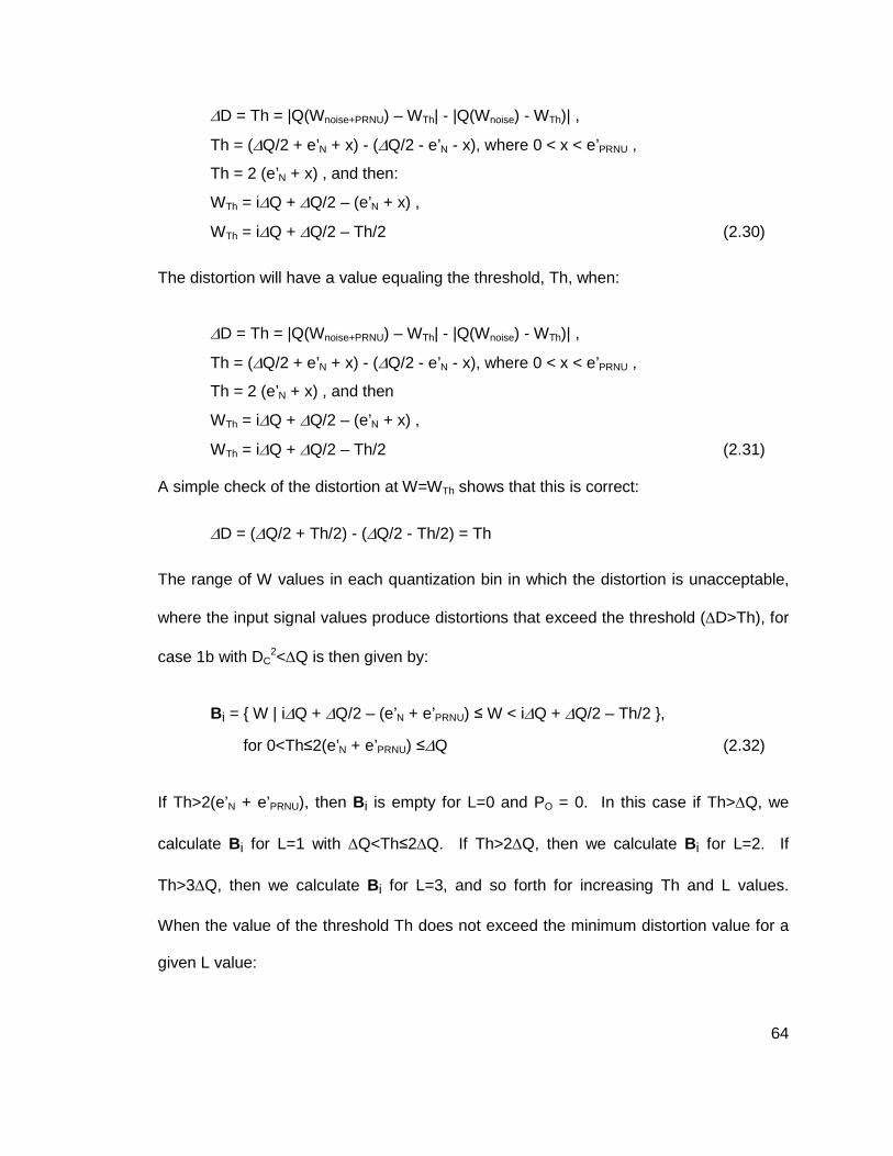
64

∆D = Th = |Q(Wnoise+PRNU) – WTh| - |Q(Wnoise) - WTh)| ,

Th = (∆Q/2 + e’N + x) - (∆Q/2 - e’N - x), where 0 < x < e’PRNU ,

Th = 2 (e’N + x) , and then:

WTh = i∆Q + ∆Q/2 – (e’N + x) ,

WTh = i∆Q + ∆Q/2 – Th/2 (2.30)

The distortion will have a value equaling the threshold, Th, when:

∆D = Th = |Q(Wnoise+PRNU) – WTh| - |Q(Wnoise) - WTh)| ,

Th = (∆Q/2 + e’N + x) - (∆Q/2 - e’N - x), where 0 < x < e’PRNU ,

Th = 2 (e’N + x) , and then

WTh = i∆Q + ∆Q/2 – (e’N + x) ,

WTh = i∆Q + ∆Q/2 – Th/2 (2.31)

A simple check of the distortion at W=WTh shows that this is correct:

∆D = (∆Q/2 + Th/2) - (∆Q/2 - Th/2) = Th

The range of W values in each quantization bin in which the distortion is unacceptable,

where the input signal values produce distortions that exceed the threshold (∆D>Th), for

case 1b with DC2<∆Q is then given by:

Bi = { W | i∆Q + ∆Q/2 – (e’N + e’PRNU) ≤ W < i∆Q + ∆Q/2 – Th/2 },

for 0<Th≤2(e’N + e’PRNU) ≤∆Q (2.32)

If Th>2(e’N + e’PRNU), then Bi is empty for L=0 and PO = 0. In this case if Th>∆Q, we

calculate Bi for L=1 with ∆Q<Th≤2∆Q. If Th>2∆Q, then we calculate Bi for L=2. If

Th>3∆Q, then we calculate Bi for L=3, and so forth for increasing Th and L values.

When the value of the threshold Th does not exceed the minimum distortion value for a

given L value:

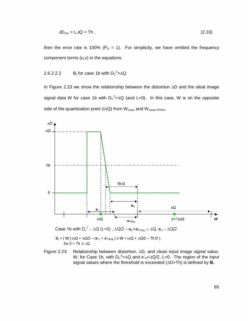
65

∆Dmin = L∆Q > Th , (2.33)

then the error rate is 100% (PO = 1). For simplicity, we have omitted the frequency

component terms (u,v) in the equations.

2.6.2.2.2 Bi for case 1b with DC2>∆Q

In Figure 2.23 we show the relationship between the distortion ∆D and the ideal image

signal data W for case 1b with DC2>∆Q (and L=0). In this case, W is on the opposite

side of the quantization point (i∆Q) from Wnoise and Wnoise+PRNU.

Figure 2.23: Relationship between distortion, ∆D, and clean input image signal value, W, for Case 1b, with DC

2>∆Q and e’N<∆Q/2, L=0. The region of the input signal values where the threshold is exceeded (∆D>Th) is defined by B i.

66

From the figure, we see that the maximum distortion of Emax = ∆Q (∆Q=2(e’N+e’PRNU))

occurs when W has the value that corresponds to Wnoise+PRNU just entering the next

quantization bin (as with the previous case):

At Wnoise+PRNU = W + e’N + e’PRNU = i∆Q + ∆Q/2, and

W = i∆Q + ∆Q/2 – (e’N + e’PRNU), and we have

∆D = |Q(Wnoise+PRNU) – W| - |Q(Wnoise) - W)|

∆D = (∆Q/2 + e’N + e’PRNU) - (∆Q/2 - e’N - e’PRNU)

∆D = 2 (e’N + e’PRNU) = ∆Q (2.34)

The range of W values in each quantization bin for which the distortion is unacceptable

(∆D>Th) is dependent upon e’N, and is examined next.

2.6.2.2.2.1 Bi for case 1b with DC2>∆Q and e’N < ∆Q/2

If e’N is less than ∆Q/2, the distortion remains constant at ∆Q as W increases until it

reaches the quantization mid-point location (i∆Q + ∆Q/2). The distortion then decreases

to a value of zero at a W value corresponding to Wnoise just entering the next quantization

bin (as was true for DC2<∆Q):

W = i∆Q + ∆Q/2 – e’N, and e’N < ∆Q/2 , we have

∆D = 0 (2.35)

The point at which the distortion matches the threshold value is the same as in the

DC2<∆Q case:

∆D = Th = |Q(Wnoise+PRNU) – WTh| - |Q(Wnoise) - WTh)| , and e’N < ∆Q/2 , for

WTh = i∆Q + ∆Q/2 – Th/2 (case 1b, DC2 > ∆Q and e’N < ∆Q/2) (2.36)

67

This gives us the same range of W values in each quantization bin for which distortion is

unacceptable, where input signal values produce distortions that exceed the threshold

(∆D>Th), for case 1b with DC2>∆Q and e’N < ∆Q/2 as for the case 1b with DC

2<∆Q:

Bi = { W | i∆Q + ∆Q/2 – (e’N + e’PRNU) ≤ W < i∆Q + ∆Q/2 – Th/2 },

for 0<Th≤∆Q (which is different from the previous case). (2.37)

If Th>∆Q, then Bi is empty for L=0. In this case we calculate Bi for L=1. If Th>2∆Q, then

we calculate Bi for L=2, and so forth.

2.6.2.2.2.2 Bi for case 1b with DC2>∆Q and e’N > ∆Q/2

If e’N is greater than ∆Q/2, as shown in Figure 2.24, the distortion remains constant at

∆Q as W increases (from the value of i∆Q + ∆Q/2 – (e’N + e’PRNU) shown in Section

2.6.2.2.2) until it reaches the value of i∆Q + ∆Q/2 - e’N. At which point Wnoise just enters

the next quantization bin, and the distortion becomes instantaneously zero:

W = i∆Q + ∆Q/2 – e’N and e’N > ∆Q/2 , we have

∆D = 0 (2.38)

This gives us a different range of W values in each quantization bin which the distortion

is unacceptable, where the input signal values produce distortions that exceed the

threshold (∆D>Th), for case 1b with DC2>∆Q and e’N > ∆Q/2:

Bi = { W | i∆Q + ∆Q/2 – (e’N + e’PRNU) ≤ W < i∆Q + ∆Q/2 – e’N },

for 0<Th≤∆Q (2.39)

68

Again, if Th>∆Q, then Bi is empty for L=0. In this case we calculate Bi for L=1. If

Th>2∆Q, then we calculate Bi for L=2, and so forth.

Figure 2.24: Relationship between distortion, ∆D, and clean input image signal value, W, for Case 1b, with DC

2>∆Q and e’N>∆Q/2, L=0. The region of the input signal values where the threshold is exceeded (∆D>Th) is defined by B i.

2.6.2.2.3 Bi for case 2b

The case 2b situation will be similar to the case 1b situation with L=1 and 0<Th≤2∆Q.

We will have the same three situations of distortion variation with W as we saw with case

2b, depending on the position of W relative to the mid-bin point when Wnoise+PRNU just

enters a bin. For case 2b, Wnoise+PRNU is two bins removed from W, and Wnoise is one bin

removed (giving us L=1). In Figure 2.25 we show the part of the distortion plot for case

2b with DC2>∆Q when L=0 and 0<Th≤∆Q.

69

Figure 2.25: Relationship between distortion, ∆D, and clean input image signal value, W, for Case 2b, with DC

2>∆Q and 0<Th≤∆Q, L=0.

2.6.2.2.4 Global error rate equation

With the range of W for unacceptable distortion (Bi) determined, we are now in a position

to solve the integral equation for the error rate, PO. However, we still need to provide a

threshold and the probability density functions (pdf) for the input image signal (W) and

the noise signals that have been operated on by the system (e’N and e’PRNU). We will

use statistical information based on appropriately selected test images and the use of

our pixel and imager system models in order to determine fW(W), feN(eN), and

fePRNU(ePRNU). The threshold value itself will be a function of these probability density

functions as well as the image system model (image processing and quantization

levels). The derived error rate equation allows us to calculate PO(u,v) for frequency

component (u,v). We must test each frequency component of a block (64 components

70

per block). As was done in [12], we must combine the individual values PO(u,v) into a

global PO using the summation law:

PO = 1 - ∏=

N

u 1∏

=

N

v 1

{1 - PO(u,v)} (2.40)

This equation can then be used in the simulation of error rate calculation using known

signal and noise statistical models. The simulation can be used to yield a mapping from

fe’PRNU(e’PRNU) to error rate, and will only have to be performed a handful of times per

sensor design. Thus, overall complexity is not a major concern. However, some

computation complexity and time can be saved by assuming, as was done in [12], that

PO(u,v) will be small for all of the frequency components (u,v), so that we can use the

approximation:

PO ≈ ∑=

N

u 1∑=

N

v 1PO(u,v) (2.41)

2.6.3 PRNU Distortion Testing Methodology

Two different sensor PRNU testing methodologies, a Monte Carlo simulation solution

and a probability model-based simulation solution, will now be developed and discussed.

Both of these methodologies will permit sensors to be tested for different applications.

We will be able to take advantage of a sensor application having a certain set of

magnitudes of quantization and ISO operating conditions. This will allow us to select

sensors for different applications using the performance in our proposed PRNU

screening methods. These methods permit us to choose operating conditions and

71

quantization levels to mask the perceptual effects of the corresponding PRNU. We will

also show how these two methodologies result in solutions that are almost identical.

2.6.3.1 PRNU Distortion Monte Carlo Testing Methodo logy

We can now state a methodology for PRNU distortion testing using a Monte Carlo

approach. The distortion measurements DC1 and DC

2 are determined for the entire

image of DCT terms. Then the difference measurements in these distortions are

calculated, yielding our error significance metrics (∆D). This is the perceptual distance

between Q(Wnoise) and Q(Wnoise+PRNU), similar to that defined in [13]. Each 8x8 DCT pixel

block of the sensor is then tested to determine if any of its 64 coefficients exceed the

visibility thresholds ( Th(u,v) ) [89], [35]. This testing is done for both the luminance and

chrominance data (Y, U, V, or Y, Cr, Cb channels). The error rate (PO), or probability of

block error, is determined using these measurements as a function of the PRNU

probability density function, DCT quantization matrices used, the sensor operating

conditions (electrons per DN or ISO number) that affect the sensor noise models, and

the camera system image processing. The definition of error rate is taken from [12] and

[13], which states that it is the probability that a DCT block will have at least one

coefficient error that exceeds the defined threshold. Acceptability is defined as the

percentage of blocks that have errors that can be tolerated. Input PRNU pdf, PRNUpeak-

to-peak, or PRNUrms values are then correlated to the final error rates for a prescribed set

of camera operating conditions. Multiple camera operating conditions can be used,

which can correspond to different camera applications. We perform this analysis using a

predetermined set of test images selected based on the camera application. A diagram

of the testing methodology is shown in Figure 2.26.

72

2.6.3.2 PRNU Distortion Model-Based Simulation Test ing Methodology

We can use Equation (2.27) of Section 2.6.2.2, along with pdfs of each DCT coefficient

component for the input image and camera system processed noise terms, to calculate

a table of error rates based upon the input parameters of operating conditions and

PRNU values (σPRNU). We modify the error rate equation to operate in the discrete

(sampled) domain instead of the continuous domain (summations used instead of

integrals):

PO(u,v) = ∑PRNUe

∑Ne

∑UBi

pmfePRNU(ePRNU)(u,v)pmfeN

(eN)(u,v)pmfW(W)(u,v) (2.42)

In using the above error rate equation, we are reminded that the set of intervals of W

values in each quantization bin which the distortion is unacceptable (UBi) is a function of

the acceptable distortion threshold ( Th(u,v) ) for each DCT frequency coefficient (u,v).

Additionally, we must apply the error rate equation for the three output channels of W

(one luminance and two chrominance, e.g., YUV). Standard PRNU testing is then used

to measure a PRNU error metric, such as block PRNUpeak-to-peak or σPRNU, for a set of

sensors. This measured PRNU error is correlated with a camera system processed

PRNU noise (e’PRNU) pdf curve (fe’PRNU()). Then the error rates for each sensor can be

determined for different applications based on the measured PRNU block values.

2.7 Performance Measurements and Conclusions

In our proposed PRNU testing methods, we use Monte Carlo simulations and probability

model-based simulations to create plots that relate measurements of raw block PRNU

73

values to failure rates for particular sensor applications. The failure rate curves are

constructed for specific sensor operating conditions (gain setting, exposure time, etc.)

and image processing settings. Each of these settings or groups of settings can be

associated with a specific sensor application. The analysis path of our proposed Monte

Carlo PRNU screening method is depicted in Figure 2.26, which shows the use of our

sensor and camera models. A set of application appropriate images is used as input to

the Monte Carlo simulations. We used over 50,000 8x8 pixel blocks to run through the

Monte Carlo PRNU screening method and to generate probability data for the probability

model-based simulation method. One of the input images used is shown in Figure 2.29.

The industry standard or conventional PRNU screening threshold value for the block

PRNU peak-to-peak limit is a heuristic and subjective visualization limit. In the results

presented in this thesis, we have used a conventional PRNU peak-to-peak testing

threshold value of 10% to define PRNU block failure. This value is fairly typical for low

and mid quality consumer applications [17]. It is a simple matter to use a different

threshold value in our method.

We show the PRNU failure rates for the conventional peak-to-peak method (black curve)

and our two proposed methods for different sensor gain settings (conversion factors of

28, 7, and 2.8 e-/DN) in Figure 2.27. The failure rate, shown on the Y-axis, is plotted in

log scale as a function of the mean block PRNUrms value (σgain/µgain). This mean block

PRNUrms value can be related to a maximum block PRNUP-P value, as shown in Figure

2.4. As sensor gain is increased, the conversion factor (e-/DN) decreases. The so

called ‘base’ or good quality compression settings were used in the calculations for

Figure 2.27. The JPEG DCT quantization matrices for the base setting are shown at the

74

end of the section in Table 2.6. These matrices can be scaled using a ‘Quant Factor’ to

increase compression, where the ‘base’ setting has ‘Quant Factor’=1.

The conventional PRNU screening method is fairly independent of the sensor gain

settings used. This is due to the conventional method removing temporal noise through

frame averaging. In actuality, the gain setting would affect the point on the pixel

response curve (see photon transfer curve of Figure 2.12) where the measurements are

made. Higher gain settings would force us to the left and down the pixel response curve

(Figure 2.12). But when temporal noise is removed, we should measure the same pixel

response variation to mean response ratio, so the conventional screening method will

have the same failure rate curve for all of these simulated gain settings. In contrast,

since our proposed method uses HVS visibility of PRNU as a distortion threshold, we will

see different failure rate curves for different sensor gain settings.

Our sensor model has a base gain of 28 e-/DN, which provides the lowest noise and

highest SNR sensor operation. Under this operational setting, the visibility of PRNU will

be the greatest. Figure 2.27 shows that at the sensor base gain setting combined with

typical DCT quantization (‘Quant Factor’=1), the conventional and our proposed PRNU

screening methods have similar sensor block PRNU variation values at which the failure

rate becomes non-zero (0.001%). This is the point at which we define the sensors as

beginning to fail the PRNU screening test. This state is shown as the failure rate knee

point, circled in the plot. This agreement suggests that the PRNUp-p threshold limit (10%

used in this case, which corresponds to a block mean σPRNU=1.5% for approximately

5100 8x8 blocks) can be determined by subjective visual analysis of images taken from

75

the sensor operating under its best (most severe) gain setting combined with typical

JPEG compression.

The conventional threshold is not finely tuned for the complete camera system, which

includes consideration of the image processing pipeline, compression, and system

noise. Furthermore, the conventional threshold does not vary with these camera

settings. We also note that the sensitivity of the conventional PRNU screening method

to the input mean block PRNU amount is greater than that of our proposed method.

This can be seen by comparing the slopes of the PRNU failure rate curves of Figure

2.27. Our proposed method produces a more gradual PRNU failure rate response to

changes in the mean block PRNU amount, which becomes flatter as the sensor gain

setting is increased (e-/DN decreases). This flattening can be advantageous, in that

slight errors in PRNU measurements become less important, and lead to smaller errors

in the failure rate calculation. Our proposed PRNU failure rate curve method is less

sensitive to changes in PRNU since we consider the entire camera system (total noise,

compression, image processing), and not just the measured block PRNU value.

We see in Figure 2.27 that the failure rate knee point will move to the right as the sensor

gain setting is increased (and e-/DN decreases). This is due to the total noise increasing

and the SNR decreasing, allowing more PRNU noise. As the sensor base gain setting is

increased (representing worse noise performance), the PRNU failure rate curve moves

to the right. This results in a lower sensor failure rate for a given PRNU variation

(standard deviation). However, at lower gain settings, we approach the point where the

DCT quantization noise will be dominant. At this point, lowering the sensor gain setting

will have little effect on the failure rate curve. We can see this affect in Figure 2.27 by

76

looking at the relatively small movement between the sensor e-/DN=7 and e-/DN=28

curves compared to the e-/DN=2.8 and e-/DN=7 curves.

In Figure 2.28, we show how the DCT quantization setting affects our proposed PRNU

failure rate method. Failure rate curves are shown in Figure 2.28 for a sensor gain

setting of 28 e-/DN combined with the cases of ‘Quant Factor’ DCT factor values of 1,

1.5, 2, and no quantization applied. The plot shows how the failure rate curves shift to

higher allowable mean block PRNU values as the DCT quantization is increased. This is

due to the PRNU becoming less significant to the measured distortion as the

quantization noise increases. The decrease in the sensor PRNU failure rate for a given

mean block PRNU value as quantization is increased is significant. This shows that for

applications with higher compression and lower image data rate transmission

requirements, we can reduce the PRNU rejection rate of sensors. When we do not

apply DCT quantization, the failure rate knee point decreases, and the failure rate curve

moves to the left. The left-most curve in Figure 2.28 shows the sensor being operated at

its highest conversion gain setting combined with no compression being applied, both of

which reduces the masking of PRNU. However, this mode of sensor operation is not

typical for lower and middle quality consumer CMOS sensors. The conventional

heuristic PRNU threshold for these types of sensors is determined with the sensor

operating under some degree of compression.

From the PRNU failure rate curves, we see several basic trends:

1) As the gain setting of the sensor is increased, a greater block PRNU error

can be tolerated (see Figure 2.27). This is due to the other sources of

noise increasing relative to the PRNU noise. The relative contribution of

PRNU to the total overall distortion is reduced, and the allowable

77

distortion threshold is increased. The operation range of the pixel is

reduced, removing some upper response region, which is more significant

for PRNU.

2) As the JPEG DCT quantization is increased, a greater block PRNU error

is allowed (see Figure 2.28). Thus, for higher compression and lower

image data transmission rates, more block PRNU error is tolerable. This

is due to the quantization noise increasing, and masking the PRNU. At

lower gain settings (low ISO, high SNR), there is little separation between

the failure rate curves when DCT quantization (compression) is applied

(see Figure 2.27). This is due to the non-PRNU noise values not being

high enough to improve the allowable PRNU failure rate. Thus, only the

DCT coefficient error visibility thresholds affect the distortion thresholds,

and the ∆D distortion is mostly due to the PRNU corruption. When no

DCT quantization is applied, lower gain settings will continue to produce

lower failure rate curves (shifted to the left), since distortion will be almost

entirely due to PRNU corruption. Often, conventional PRNU testing does

not consider these more severe operating conditions for a sensor, since

they do not occur during typical camera operation. Thus, the heuristic

block PRNU threshold is set higher (commonly PRNUP-P block threshold

of 10% [16]), since it assumes a minimum amount of compression will be

used.

3) Though not directly shown in the plots, more severe image processing

can result in less block PRNU error being tolerated. This image

processing includes color correction and saturation enhancement. Other

image processing, such as Bayer pattern interpolation, which may low

pass filter image data, can result in more block PRNU variation being

tolerated. To understand the net effect of the image processing, a

complete model must be simulated. The Monte Carlo analysis used

image signal probability distributions taken at the output of the camera

system model. The probability model-based simulations used the image

processing system model to create the DCT block-wise models.

78

4) The conventional ‘common’ allowable PRNU peak-to-peak threshold of

10% [16] for low to mid quality consumer sensors roughly corresponds to

the knee in the proposed PRNU screening method failure rate curve for

our sensor operating at its base gain combined with base JPEG

compression (matrices values in Table 2.6) and standard image

processing. This point is shown in Figure 2.27. A mean block PRNUrms

value of 1.5% corresponds to a maximum block PRNUP-P value of 10% for

a sensor with approximately 300K to 1M pixels. We would expect the

methods to be in close agreement for the most severe and realistic

operating conditions.

5) The conventional PRNU peak-to-peak failure rate method is very sensitive

to the PRNU threshold parameter. This can be seen in the very steep

curves of the conventional PRNU failure rate shown in Figures 2.27 and

2.28. Our proposed method produces PRNU failure rate curves that have

a more gradual response to changing block PRNU values than the

conventional method. This can lead to a more stable PRNU metric, which

is less sensitive to errors in block PRNU measurements. This reduced

sensitivity is due to consideration of the entire camera system (total noise,

compression, image processing).

6) The Monte Carlo and probability model-based simulation methods

produce nearly identical error rate performance results. This is due to the

use of the same underlying pixel and camera models, as well as the use

of the same distortion and threshold methodologies.

We can use our proposed method to create a full set of failure rate curves for a sensor

family. Subsets of the curves can then be assigned to different sensor applications. We

can then screen sensors using the standard method of measuring PRNU block values.

These measured values then are used with the new failure rate curves to determine

failure rates for the different sensor applications. This is the classification of sensors

based on their PRNU performance and the requirements of specific applications. We

79

use the idea that different sensor applications will have different requirements on

quantization (compression) amounts, acceptable SNR, image processing applied,

sensor gain settings, and other operating conditions. With this methodology, the yield

rate of sensors can be increased. In order to determine quantitatively the potential yield

rate improvement, we need to acquire more data on industry established acceptable

PRNU block thresholds and failure rates per sensor. One difficulty we find is that much

of this information is company proprietary. Thus, the task of calculating the yield rate

improvement from the use of our PRNU method requires further study.

80

F

igur

e 2.

26:

Ana

lysi

s pa

th (

Flo

w D

iagr

am)

of p

ropo

sed

PR

NU

Mon

te C

arlo

dis

tort

ion

scre

enin

g m

etho

d.

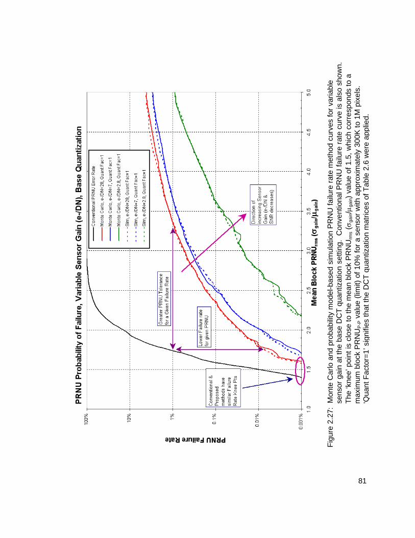
81

Fig

ure

2.27

: M

onte

Car

lo a

nd p

roba

bilit

y m

odel

-bas

ed s

imul

atio

n P

RN

U fa

ilure

rat

e m

etho

d cu

rves

for

varia

ble

se

nsor

gai

n at

the

base

DC

T q

uant

izat

ion

setti

ng.

Con

vent

iona

l PR

NU

failu

re r

ate

curv

e is

als

o sh

own.

The

‘kne

e’ p

oint

is c

lose

to th

e m

ean

bloc

k P

RN

Urm

s (σ

gain/µ

gain)

valu

e of

1.5

, whi

ch c

orre

spon

ds to

a

m

axim

um b

lock

PR

NU

P-P

val

ue (

limit)

of 1

0% fo

r a

sens

or w

ith a

ppro

xim

atel

y 30

0K to

1M

pix

els.

‘Qua

nt F

acto

r=1’

sig

nifie

s th

at th

e D

CT

qua

ntiz

atio

n m

atric

es o

f Tab

le 2

.6 w

ere

appl

ied.

82

Fig

ure

2.28

: P

RN

U fa

ilure

rat

e cu

rves

for

sens

or g

ain

setti

ng o

f e-/

DN

=28

(ba

se g

ain)

and

var

iabl

e w

ith v

aria

ble

DC

T

qu

antiz

atio

n ap

plie

d. ‘

Qua

nt F

acto

r’ is

the

mul

tiplic

ativ

e te

rms

appl

ied

to th

e JP

EG

DC

T q

uant

izat

ion

mat

rices

sho

wn

in T

able

2.6

. T

he fa

r le

ft cu

rve

is th

e ca

se w

here

DC

T q

uant

izat

ion

was

not

app

lied

and

the

low

est g

ain

setti

ng w

as u

sed.

Thi

s ca

se is

sev

ere,

and

is n

ot ty

pica

lly u

sed

for

dete

rmin

ing

PR

NU

failu

re.

83

Fig

ure

2.29

: S

ampl

e im

age

used

or

Mon

te C

arlo

PR

NU

scr

eeni

ng m

etho

d an

d to

gen

erat

e pr

obab

ility

dat

a fo

r th

e

pr

obab

ility

mod

el-b

ased

sim

ulat

ion

met

hod.

84

Table 2.6: Luminance [Y] and Chrominance [Cr & Cb] quantization matrices.

85

Chapter 3

Bayer Cross-Talk Reduction Method for

Embedded Imaging Systems

3.1 Introduction

In this chapter we develop a simple multi-channel imager restoration method to correct

color channel dependent cross-talk of a Bayer color filter array (CFA) sensor. In this

effort, we break up each color channel into color channel components (CCC) and create

separate cost functions (weakened optimization) for each CCC. Our restoration solution

has its regularization parameters determined by maximizing the developed local pixel

SNR estimations (HVS detection constraint), where local pixel adaptivity is applied. We

utilize sensor characterization a priori information in our solution. The correction method

is geared towards implementation into the on-chip digital logic of low-cost CMOS

sensors. Thus, our solution is a direct and computationally simple technique.

The different sources of pixel cross-talk are discussed in Section 3.2.1. The general

Bayer cross-talk problem which we must solve is presented in Section 3.2.2. The basic

constrained least squares (CLS) problem solved by our method is presented in Section

86

3.2.2.1. In Section 3.2.2.2, color channel components are defined and their use in our

solution is discussed. In Section 3.2.3, existing restoration methods that have been

applied or could be applied to the Bayer cross-talk problem are discussed. The

inadequacies of applying these methods to meet the particular requirements or

constraints of our low-cost camera system are discussed in that section. The goals,

requirements and constraints of our low-cost camera system Bayer cross-talk correction

method are presented in Section 3.2.4. The motivation for our novel solution to the

Bayer cross-talk problem is presented in Section 3.3.1. The general approach of

methods that we use to address the inadequacies of existing restoration methods are

developed in Section 3.3.2. In Section 3.4, we derive our deterministic separate CCC

constrained least squares local SNR (SCLS SNR) method. Lastly, performance data

and conclusions are presented in Section 3.5.

3.2 Bayer Cross-Talk Problem

3.2.1 Causes of Bayer Multi-Channel Blurring

Image sensor cross-talk is the loss of electrons or photons from a pixel to neighboring

pixels. Pixel cross-talk degrades both image sharpness (modulation transfer function,

MTF) and colorimetric accuracy (highly de-saturated, color-muted images). There are

both photonic (optical) and electronic (lateral diffusion) forms of cross-talk, as shown in

Figure 3.1. Photons can pass at an oblique angle through the CFA of one pixel such

that they are collected by an adjacent pixel with a different color filter. After carriers

have been created by photons in a photodiode, they may diffuse to the depletion region

of an adjacent pixel. The depth that photons penetrate into the photodiode before

creating an electron-hole pair is wavelength dependent [9]. Photons of shorter

87

wavelength (e.g., blue light) have greater photon energy, and excite the silicon's

electrons sooner. They will not penetrate deep into the photodiode. Thus, blue pixels

will experience less diffusion cross-talk loss. Photons of longer wavelength (e.g., red

light) penetrate deeper into the photodiode. The carriers created by these photons are

more likely to diffuse to neighboring pixels. The percentage of cross-talk will increase as

the size of pixels is progressively reduced.

Figure 3.1: Photonic and electronic forms of pixel cross-talk.

The Bayer pattern, shown in Figure 3.2, is the most commonly used CFA for low-cost

sensors. For imagers that use the Bayer CFA pattern, there will be a larger degree of

cross-talk from red pixels to green pixels than other color combinations. Additionally,

due to asymmetric pixel lay-outs, the amount of cross-talk signal received by green

pixels on odd and even rows can be different. The color pixel type dependencies of

cross-talk make it a Bayer multi-channel blurring problem. Both the optical and diffusion

cross-talk can be characterized for a sensor design, and then used for its correction.

88

Typical values of cross-talk coefficients for a CMOS sensor with small pixels [17] are

shown in Figure 3.3. From Figure 3.3, we see that the extent of the cross-talk blurring

matrices is small (typically within a 5x5 pixel area).

Figure 3.2: Bayer CFA pattern (typical types: red, green-even, green-odd, blue).

Figure 3.3: Cross-talk loss coefficients for a typical small pixel CMOS sensor [17].

3.2.2 Bayer Multi-Channel Blurring Problem Formulat ion

The Bayer multi-channel cross-talk problem can be viewed as a blurring restoration

problem with four channels: green-odd, red, green-even, and blue (Go, R, Ge, B). We

can assume without loss of generality that each of the N=4 color channels has M×M or

M2 pixels. The Bayer cross-talk blurring problem can be written in stacked vector and

matrix form as:

y = H f + n , (3.1)

89

where y is the NM2×1 observed blurred image with additive noise vector, f is the NM2×1

input (non-corrupted) image vector, n is the NM2×1 noise image vector, and H is the

NM2×NM2 multi-channel blurring matrix. We can write the y, f, and n vectors for the

Bayer color channels as:

=

B

Ge

R

Go

y

y

y

y

y ,

=

B

Ge

R

Go

f

f

f

f

f ,

=

B

Ge

R

Go

n

n

n

n

n (3.2)

The Bayer CFA multi-channel blurring matrix (H) can be written as:

=

BBGeBRBGoB

GeBGeGeRGeGoGe

RBGeRRRGoR

GoBGeGoRGoGoGo

HHHH

HHHH

HHHH

HHHH

H , (3.3)

where the full blurring matrix H is composed of stationary block-circulant M2×M2 sub

matrices Hji. The sub matrices Hji are defined as having the j index being the input

channel and the i index being the output (blurred) channel. Thus, HRGe would represent

the blurring of the green-even channel due to the red channel. The assumption of a

stationary block-circulant cross-talk blurring matrix is usually valid for our target camera

system, as can be seen from characterization data of sensor cross-talk [17]. However,

stationarity can be sometimes be invalidated by optical effects resulting from low-cost

lenses and small pixels. We will not consider these optical non- stationary effects in this

thesis.

Numerous multi-channel deterministic regularization methods have been developed.

Many of these methods are non-linear and require iterative solutions. Other solutions

90

make simplifying assumptions such as neglecting the dependence between the color

channels, not considering the full spatial blurring, or not being adaptive to the local noise

levels. The most popular and practical restoration methods are discussed in Section

3.2.3. We employ a direct deterministic regularization estimation method, which we

discuss in Section 3.2.2.1 as part of our problem formulation.

3.2.2.1 Constrained least squares solution

A widely accepted deterministic regularization method is constrained least squares

(CLS) restoration [5]. CLS methods minimize a linear operator on the estimated

restored image f̂ (such as Qf̂ ) subject to some set of conditions [3]. The operator Q is

the regularization functional, which reduces the effects of the small singular values of H

that occur at high frequencies, while leaving the larger ones unchanged. One popular

choice for the known condition is the norm of the noise signal (||n||2). Using this

approach, along with the smoothness constraint, ||Qf̂ ||2, the constrained optimization

problem can be written as determining a solution f̂ which [27]:

minimizes: || Qf̂ ||2 ,

subject to the constraint: || y – Hf̂ ||2 = || n ||2 (3.4)

This can be solved using a Lagrangian technique, that is obtaining f̂ so as to minimize

the cost function [5], [27]:

φ(f̂ , β) = (|| y – H f̂ ||2 - || n ||2) + β || Q f̂ ||2 , (3.5)

where the Lagrange multiplier, or regularization parameter, β, is adjusted in order to

meet the defined constraint or set of constraints [5]. Estimates of the signal (f) and noise

91

(n) energy values can be used to determine β [5], [26], [27]. Iterative methods are often

used in order to determine the optimal value of β [5], [27]. For our direct solution, we

use sensor characterization noise models that are signal-dependent in order to calculate

restored pixel SNR estimates (refer to Section 3.4.2.2). We determine the optimal

regularization parameter value by maximizing the estimates of the corrected pixel SNR

using an off-line search method (see Section 3.4.2.2.4):

β = maximize: || f̂ 2 / ň2 ||2 , (3.6)

where f̂ is the estimated restored pixel value, and ň is the estimated noise value. Our

problem is further defined to operate on color channel components, as discussed in the

Section 3.2.2.2. The local pixel SNR optimization is derived in Section 3.4.2.2.4.

3.2.2.2 Separation of color channel components

For the Bayer CFA (see Figure 3.2), the color channel components (CCC) are defined

as being each of the four-color channels that compose each color channel. All four color

channels are components of each blurred color channel. During reconstruction, each

CCC is corrected. Thus, referring to Equations (3.2) and (3.3), we can write each output

(observed) blurred channel i as:

y i = HGoi fGo + HRi fR + HGei fGe + HBi fB , or

y i = yGoi + yRi + yGei + yBi (3.7)

The vector yi is defined as a color channel, and the vector terms Hji f j and yji (e.g., HGoi

fGo and yGoi) are defined as CCCs. The matrix Hji operates on channel j (f j) to produce

92

y ji, which corrupts channel i, where i and j belong to the set {Go, R, Ge, B}. Likewise, we

can define each reconstructed channel i as:

f̂ i = AGoi yGo + ARi yR + AGei yGe + ABi yB (3.8)

The Aji matrices are defined as the color channel correction matrices for color channel i.

For example, AGoi corrects the color channel Go component of color channel i. Each

vector term Aji y j (e.g., AGoi yGo) is a CCC vector term of the reconstructed color channel

vector f̂ i.

Applying the CLS solution from the Section 3.2.2.1 to each CCC term (see Section 3.4.1

for details), our constraints for our separated CCC CLS (SCLS) problem are:

minimize: || Qji f̂ ji ||2 ,

subject to the constraint: || y j – Ĥji f̂ ji ||2 = || ň j ||

2 , (3.9)

where f̂ ji is the restored CCC value, and the optimal regularization parameter values, βji,

are determined by using an off-line search method (see Section 3.4.2):

βji = maximize: || f̂ ji 2 / ň j

2 ||2 (3.10)

Thus, our problem formulation consists of the constraints of Equation 3.9x combined

with using Equation 3.10x to determine the regularization parameter values. Equations

(3.9) and (3.10) are further simplified to scalar form to operate over local pixel areas, as

discussed in Section 3.4.2.

The use of SCLS simplifies the Bayer cross-talk problem (Equations (3.1), (3.2), (3.3)

and (3.4)) and allows for a direct solution. However, it neglects the correlation of the

93

errors between different CCC components and introduces an error which will be image

dependent. We also use the approximation that the sum of the separately minimized

CCC cost function terms will be the minimum of the sum of the cost function terms

(weakened optimization). These errors are examined in Section 3.4.1.2. The SCLS

simplification benefits outweigh the relatively small errors from an exact solution.

3.2.3 Examination of Existing Image Blurring Soluti ons

We review single channel blurring restoration in Section 3.2.3.1. We then examine

multi-channel blurring in the Section 3.2.3.2. More details on multi-channel blurring

restoration methods can be found in Appendix C.

3.2.3.1 Inverse Filtering Problem

A direct solution of the simple degradation problem shown in Figure 3.4 can be found by

solving for an estimate f̂ which minimizes the Euclidean norm:

min || y – Hf̂ ||2 (3.11)

Figure 3.4: Simple blurring and additive noise problem.

This is a least squares fit to the data, and leads to the generalized inverse filter

(unconstrained) solution:

f̂ = (HTH)-1 HT y , (3.12)

Low Pass Filter h f y

n

94

with H being the matrix form of the convolution filter h. When a stationary model is used,

H is block circulant and can be diagonalized with the use of the 2-D DFT. This is due to

the eigenvalues of a block circulant matrix being the 2-D discrete Fourier coefficients of

the impulse response of the degradation system, and the eigenvectors being the

complex exponential basis functions of this transform [5]. We can write in matrix form:

H = WHW-1 , (3.13)

where H is a diagonal matrix comprising the 2-D DFT coefficients of H, and W-1 is a

matrix containing the components of the complex exponential basis functions of the 2-D

DFT. Using the DFT properties of block circulant matrices, the solution can be written in

the discrete frequency domain as:

F(l) = H*(l)G(l) / ||H(l)||2 , (3.14)

where F(l) is the DFT of the restored image, H(l) is the PSF (point spread function or

blurring) DFT, and G(l) is the observed image DFT. These terms are functions of the 2-

D discrete frequency index l, where l=(k1,k2) for k1,k2=0,…,N-1, for a NxN point DFT. In

Equation (3.14), * denotes complex conjugation. Using this method, we can solve for the

inverse matrix or an inverse convolution filter.

A significant problem with the application of Equation (3.14) is that the blurring problem

is ill-posed [82]. Because H is ill-conditioned, small bounded deviations may lead to

unbounded deviations in the solution. Thus, additional constraints are needed in order

to guarantee the uniqueness of the solution and make the problem well-posed. For the

cross-talk blurring problem, the degradation matrix H is a low pass filter, which means

that H(l) is small for l corresponding to high frequencies. Since the noise occurs at all

95

frequencies, the noise at frequencies where H(l) is near zero will be greatly amplified.

The condition number of the blurring H matrix is the ratio of its maximal and minimal

eigenvalues (non-zero values only), and is a measure of how well-posed it is. A problem

with a blurring H matrix that has a low condition number is said to be well-conditioned,

while a problem with a high condition number is said to be ill-conditioned.

Many techniques have been developed to solve this problem [5], including direct,

iterative and recursive approaches. Direct approaches to regularization in a restoration

problem can use either a stochastic or a deterministic model for the original image. The

model represents prior information about the solution that can be used to make the

problem well-posed. Stochastic regularization uses a linear filtering approach that

computes the estimate f̂ :

min E{|| f – f̂ ||2} (3.15)

Using the stochastic model for f and n requires prior knowledge of the statistics of the

image data that are then used to regularize the problem. Solving the problem using the

DFT also requires that the image and noise fields be stationary, which often is not the

case. Perhaps most importantly, costly calculations of correlations matrices for the

image and noise data must often be performed. It has been shown [93] that stochastic

solutions are very sensitive to the accuracy of the estimations of the image and noise

correlations. Because of these requirements and constraints, a stochastic regularization

approach is not desirable for a low-cost camera system. The linear estimate that

minimizes Equation (3.15) leads to the classical form of the Wiener filter:

f̂ = RffHT(HRffH

T + Rnn)-1 y , (3.16)

96

where Rff and Rnn are the correlation matrices of the image and noise data, respectively.

As discussed in Section 3.2.2.1, deterministic regularization applies prior information

about the original image for regularizing the restoration problem [31]. The Lagrangian

cost function of Equation (3.4) can be solved by performing the indicated minimization.

We take the derivative with respect to f̂ , set the result to zero and solve, giving:

f̂ = (HTH + βQTQ)-1 HTy (3.17)

The Lagrange multiplier β must be determined for the given set of constraints [5]. As

has been discussed, this often is done in an iterative fashion in order to determine the

optimal value.

3.2.3.2 Existing Bayer multi-channel blurring probl em solutions

There exist many restoration methods that can be applied to the Bayer cross-talk

problem (Equations (3.1), (3.2), and (3.3)). Due to their complexity, memory

requirements, and execution time, many of these methods cannot be implemented into

simple low-cost camera systems. Other methods in common use for low-cost systems

do not adequately correct the image data. We present some of the more important and

commonly used restoration methods for Bayer multi-channel blurring in the sections

which follow. More details on these methods can be found in Appendix C. Additionally,

more restoration methods are reviewed in Appendix C.

3.2.3.2.1 Multi-channel methods that optimize color channel regularization

The more complex multi-color channel restoration methods allow for the optimization of

the regularization parameter for each color channel separately. These restoration

97

methods typically employ an iterative solution or must use estimations of signal and

noise statistics. Two methods are developed in [27] for determining the regularization

parameter of each color channel: a set theoretic (ST) approach and a constrained least

squares (CLS) optimization. These two methods serve as the foundation for many other

methods. Both of these methods solve the multiple channel regularization equation:

[ HTΛΛΛΛH + QTQ ] f̂ = ΛΛΛΛHTy , (3.18)

where ΛΛΛΛ is a matrix of N color channel regularization parameters (λi), and is written in

the form:

λ

λ

λ

λ

=

]I[

]I[

]I[

]I[

4

3

2

1

000

000

000

000

ΛΛΛΛ , (3.19)

and where [I] is an identity matrix of size M2×M2. The regularization operator, Q, used in

[27] has both 2-D Laplacian (within channel smoothing) and 3-D Laplacian (across

channel smoothing) components. Using a Laplacian smoothing prior simplifies the

problem since it results in a quadratic regularization operator (system of linear

equations) [48]. The multi-channel blurring matrix H was defined by Equation (3.3). The

objective is to determine the optimal regularization parameters (λi) of diagonal matrix ΛΛΛΛ.

The ST approach uses a smoothness constraint for each color channel (Ei), where an

assumption of equal channel smoothness is used. This is done using an estimate of the

full original image (f) statistics. This method also requires an estimate of each color

channel’s additive noise (ei) . The regularization parameters are then determined from

these estimations. The requirement for accurate estimates of Ei and ei have been found

98

to be overly restrictive [44]. Iterative methods can be used to determine accurate

estimates for the regularization parameters [48].

A CLS optimization approach is developed in [27] for the case when the smoothness

constraint value E is not known a priori or a satisfactory estimate is not available. For

this method, we seek a solution f̂ which:

minimizes: || Qf ||2

subject to: || Hif – y i ||2 = || n i ||

2 = ei2 , for i=1,2, …, N , (3.20)

where Hi is the ith channel M2×NM2 matrix Hi=[H1i, H2i, … HNi] and n i is the noise of color

channel i. The solution of the regularization Equation (3.18) subject to these constraints,

Equation (3.20), requires that we must simultaneously find the values of λi, which can be

written as:

Zi(λ1, λ2, ... λΝ) = (|| Hi f̂ – y i ||2 = || ni ||

2) for i=1,2, …, N (3.21)

This leads to a nonlinear problem, which has a very high computational cost, since the

roots of the nonlinear functions Zi(λ1, λ2, ... λΝ) must be found simultaneously to give the

desired λi values. Typically, it is solved using an iterative method, such as Newton

iterations, to find the matrix of λi values (matrix ΛΛΛΛ) of Equation (3.19).

The solution of Equation (3.18) can be written as:

f̂ = Ây , with

 = [ HTΛΛΛΛH + QTQ ]-1 HT (3.22)

99

Then, similar to Equation (3.8), we can write the reconstructed channel i using Bayer

channel notation (Go, R, Ge, B) as:

f̂ i = Â Goi yGo + Â Ri yR + Â Gei yGe + Â Bi yB , (3.23)

and the multi-channel restoration matrix  in the Bayer CFA notation (Go, R, Ge, B) is

written as:

====

BBGeBRBGoB

BGeGeGeRGeGoGe

BRGeRRRGoR

BGoGeGoRGoGoGo

ÂÂÂÂ

ÂÂÂÂ

ÂÂÂÂ

ÂÂÂÂ

 , (3.24)

As with Equation (3.8), each vector term Âji y j of Equation (3.23) is a CCC vector term of

the reconstructed color channel vector f̂ i. We would like to find a simple, direction form

of  which satisfies our requirements of Section 3.2.4.

For both the ST and CLS methods, the amount of within-color channel smoothing and

cross-color channel smoothing applied are controlled by the same regularization

parameter. This restriction can result in sub-optimal performance, since this solution

does not consider the interaction of the channels in determining the optimal

regularization values λi for each channel. Each λi term is optimized using only its

channel noise and maximum energy estimations, but each corrected channel will be a

function of all the observed channels and all of the regularization parameters (f̂ i=Func{y,

H, Q, λi=1,4}). These methods also do not take into account the local or global difference

of values of the noise terms of the within and cross CCCs. Both of the methods in [27]

100

use global fixed noise variance values. The use of estimations and iterative steps also

make these methods too computationally expensive for our target application.

3.2.3.2.2 Simple direct solutions commonly used in low-cost imaging systems

There are several simple and direct solutions to the Bayer cross-talk blurring problem

that can be implemented in low-cost camera systems. However, they use assumptions

that limit their performance. Several of these methods are discussed in Appendix C. A

simple and common approach used in industry in to correct the signal error due to cross-

talk utilizes a 3-by-3 color matrix correction. This correction, which is representative of

methods used in low-cost camera systems, essentially performs a linear minimum mean

squared error (LMMSE) color correction. The loss of image sharpness is normally

corrected in a separate step, which typically is concerned with edge sharpness and not

inverse filtering. An optimal 3x3 color correction matrix can be determined using linear

regression [43] or calculated from sensor and lighting parameters. The 3x3 color

correction matrix TCC can be broken down into a 3x3 saturation matrix TSat and a 3x3

white balance matrix TWB that only has terms on its main diagonal, as shown:

TSat TWB = TCC ,

TTTTTTTTT

SatSatSat

SatSatSat

SatSatSat

333231

232221

131211

TT

T

WB

WB

WB

3

2

1

000000

=

TTTTTTTTT

CCCCCC

CCCCCC

CCCCCC

333231

232221

131211 (3.25)

Using this approach, the white balance matrix corrects for the ambient lighting conditions

(dynamic, scene dependent), and the TSat matrix coefficients correct for the sensor

dependent responses. These sensor dependent responses include cross-talk, as well

as the responsivity of silicon and the transmissivity of the CFA used.

101

In order to maintain the white balance of an image, the TSat matrix must have the

coefficients of each of its rows sum to one. Thus, as the magnitude of the off-diagonal

saturation terms increase, the on-diagonal terms of TSat must also increase. This means

that for sensors that have more cross-talk, the TSat coefficients will have larger values,

and the SNR of the processed images will decrease, due to amplification of the noise.

The calculations of the ideal correction coefficients for a 3x3 TSat matrix are shown in

Figure 3.5. The cross-talk coefficients for a DVGA CMOS sensor are used, where the

pixel area applied has been restricted to 3x3 pixels. In the signal diffusion table of the

figure, the amount of charge that enters a target pixel (center pixel) and ends up at the

specified pixel location is shown. This data is derived from sensor cross-talk

characterization [17].

There are several sources of error from using this approach. The mean blurred transfer

of signal from one pixel type to neighboring pixel type is used in constructing a 4x4

cross-talk transfer matrix. This forces the averaging of cross-talk that occurs in different

directions. For example, a blue pixel has four neighboring red pixels, each of which has

a particular cross-talk value. But an average cross-talk value will end up being used for

all of its red pixel neighbors. The inverse matrix operation will create a mean blurring

correction matrix. Another error is, in order to simplify the camera correction process,

the difference in green-even and green-odd pixel responsivity is not taken into account.

The correction matrix is reduced from a 4x4 matrix to a 3x3 matrix, which introduces a

bias error. The 3x3 correction matrix allows the correction to be applied to a Bayer

interpolated pixel triplet (RGB values at each pixel location). Thus, an ideal correction is

not possible with this method. By treating the green even and odd pixels the same, a

bias error is created since neither pixel type is corrected using the proper coefficients.

102

This error increases as the asymmetrical behavior of cross-talk increases. Often, simple

smoothing or median filtering is used to correct this fixed pattern error [54]. But these

methods do not correctly restore the non-blurred image values.

Figure 3.5: Calculations of the color correction matrix for a typical low-cost camera

sensor.

This method has no regularization in place, and cannot account for different noise levels.

A common industry approach is to adjust the ideal 3x3 TCC matrix to approach the TWB

matrix as the overall camera system noise increases (or the SNR decreases). Thus, the

coefficients of the saturation matrix are reduced in magnitude when higher camera

system gains are used (indicative of lower lighting levels and lower SNR). The

adjustment is very rough and global (no local effects considered). By using this adaptive

103

3x3 matrix approach, the performance at the low quality operating conditions (low light,

low SNR) is improved. The control for this adjustment is usually tied to camera

exposure time, sensor analog gain, and required digital gain. This idea is shown in

Figure 3.6 for the same camera system as defined in Figure 3.5.

3x3 Correction Matrix, TCC 3x3 White Balance Matrix, TWB

Figure 3.6: Typical low-cost camera color correction matrix adjustment.

3.2.3.2.3 Summary of limitations of existing multi- channel blurring correction methods

Simple and direct solutions to the Bayer cross-talk blurring problem, such as the ones

discussed in Section 3.2.3.2.2 and Appendix C, can be implemented in low-cost camera

systems. However, these methods use assumptions that limit their performance, such

as not correcting cross-channel blurring and not accurately correcting the spatial blurring

due to cross-talk. The more complex restoration methods examined in Section 3.2.3.2.1

and Appendix C require iterative solutions or rely on having accurate estimations of

image and noise statistics. Additionally, these regularization methods use a single

regularization parameter for all of the CCCs that compose a color channel. These

methods also do not use local pixel adaptivity based the HVS’s sensitivities and usually

do not make use of noise models which vary with signal magnitude.

104

3.2.4 Requirements and Goals of Our Solution

The goals, requirements, and constraints of our Bayer sensor cross-talk correction

method for implementation in a low-cost camera system are:

1) The correction method must be appropriate for a low-cost camera

system, which leads to limits on the required memory, operation

execution time, and chip area of implementation (complexity of

algorithm). Due to execution time limits, the correction method must

have a direct, non-iterative, non-recursive approach. Due to limited

memory and execution time, we cannot perform real-time global image

and noise estimations. We also will not be able to perform real-time

frequency domain operations or invert large matrices in the inverse

blurring solution. We would like to use a convolution, sliding filter

approach, since this matches the implementation of the other image

correction methods used in these camera systems and is relatively

simple and fast.

2) Our solution must address human visual system (HVS) sensitivities.

Specifically, the HVS’s sensitivity to local signal to noise contrast and

low-frequency color must be optimized in our solution [7], [19], [56],

[64], [73], [75], [76], [85]. Thus, we must adjust the regularization

parameters based on the HVS’s sensitivities. We wish to take

advantage of this constraint to simplify the calculations required for the

noise and image statistics used. Following these HVS requirements,

we wish to create a real-time spatial SNR adaptive solution.

3) Our restoration method must be adaptive to global operating conditions.

This requirement follows from the range of lighting and exposure time

conditions in which the camera must operate. The algorithm should

also be adaptive to local image SNR conditions (item 2 above), as is

driven by the HVS behavior [7], [19], [56], [73].

105

4) We must exploit sensor a prior characterization data. In order to use a

direct correction method, we must have accurate local pixel SNR

estimations. We will meet this goal using mean local estimations

derived from sensor characterization data. Simple noise models for the

pixels must be used to define pixel SNR behavior curves.

5) We must correct for asymmetrical behavior of cross-talk. Detailed

cross-talk characterization data must be used in correcting this blurring.

Usually, median or mean filtering is used to correct asymmetrical

blurring in low-cost camera systems. These systems do not properly

correct the green-even/green-odd pixel mismatch problem. Of course,

the wavelength dependent behavior of cross-talk (which defines the Hji

matrices) must be exploited.

6) Our method must apply an accurate white balance correction. For high

SNR operating conditions, camera systems generally apply an ideal

color correction (see Section 3.2.3.2.2). These corrections include a

white balance and a saturation correction. When the operation

conditions are poor, with low SNR, a white balance is still performed.

However, the saturation correction is reduced or skipped. Our

correction method must apply a white balance correction for all

operating conditions, but must also be adaptive to the operating SNR in

applying the saturation correction. We will later show how our use of

separate CCC correction addresses this requirement.

3.3 Proposed Solution to the Bayer Cross-Talk Probl em

3.3.1 Motivation and General Approach of Our Propos ed Solution

The general ideas of how our proposed solution addresses the various weaknesses of

existing restoration methods when applied to the Bayer cross-talk, low-cost camera

system problem are presented in this section. We listed in Section 3.2.4 the set of

requirements and constraints that we must meet. In this section, we list the general

106

approach and ideas that we will use to meet these requirements, as well as noting where

we have developed new approaches to the solution of the Bayer cross-talk problem.

1) We separate each color channel into a summation of CCCs, which

allows the separate regularization of each CCC (refer to Equation (3.7)).

This permits exploiting the different degrees of blurring filter ill-

conditioning for the CCCs and the SNR values of the color channels.

This separation also leads to significantly reducing the complexity of the

solution. No restoration methods have previously used this approach.

2) We use the local pixel SNR value to calculate the regularization

parameter. This is done to match the HVS’s sensitivity to local SNR [7],

[19], [56], [73] and low-frequency color error [64], [75], [76], [85]. We

have not seen this approach used by other restorations methods. We

make use of signal-dependent noise models, determined from sensor

characterization, to determine local pixel SNR estimations. The use of

local pixel SNR ensures good white color balance, while providing

adaptive saturation correction. It does not require expensive signal

energy calculations. Instead, a priori calculations are performed off-

line, reducing the amount of computations that must be done real time.

The use of local SNR values for each CCC allows spatially adaptive

corrections, whereas most existing methods use global regularization

values based on total image signal and noise energies.

3) We use a local mean estimate, or blurred estimate, for the local CCC

SNR values. This improves the accuracy of our estimate, while

matching the HVS’s color error and SNR sensitivity. The improved

estimate allows the use of a direct method; instead of an iterative

solution that would be too complex and take too long to run. The local

averaging process reduces the error in our local CCC SNR estimate by

smoothing the noise. Again, we make use of signal-dependent noise

models determined from sensor characterization. We have not seen

107

this locally adaptive approach combined with sensor SNR

characterization used by other restorations methods.

4) Detailed cross-talk characterization data is used to create directional

(pixel neighborhood) filters. Existing heuristic methods used in low-cost

camera systems do not address local non-symmetrical blurring and are

not locally adaptive in their corrections. They only have a gross overall

camera SNR operating condition adaptivity. These systems do not

properly correct the green-even/green-odd pixel mismatch problem.

5) Sensor characterization information is used to create simple noise

models for the pixels, which define pixel SNR behavior curves. These

noise models will be a function of the pixel signal level. This

information, along with cross-talk blurring data, is used to create off-line

look-up tables for selecting the optimal regularization parameters that

are applied on a local spatial manner across the image. This creates a

real-time spatial SNR adaptive solution. Use of sensor characterization

is not considered novel.

In our restoration method, we incorporate the HVS attribute that the probability of visual

detection is dependent upon the local SNR (contrast sensitivity of the human eye) [7].

This criteria follows from Crozier’s Law of signal probability of human detection [19],

which states that the psychometric 50% probability of detection is proportional to the

constant K = Signal/Noise = SNR. In 1948, Rose [31] used K to relate luminance

threshold to noise (SNR). As documented in [48], human visual object detectability is

proportional to image contrast and inversely proportional to background noise. We also

utilize the HVS’s attribute that the low-frequency spatial components of color lead to the

optimal color match (Schade experiments [75], [76] and extensions [64], [85]). This

shows that, for color accuracy, it is most important to have low spatial frequency data

color corrected accurately. This behavior of the HVS is depicted in Figure 3.7. Using

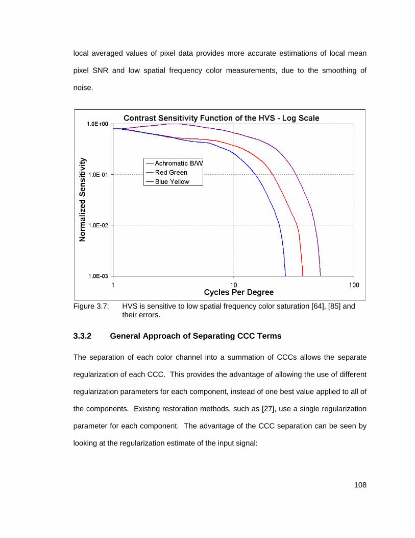
108

local averaged values of pixel data provides more accurate estimations of local mean

pixel SNR and low spatial frequency color measurements, due to the smoothing of

noise.

Figure 3.7: HVS is sensitive to low spatial frequency color saturation [64], [85] and

their errors.

3.3.2 General Approach of Separating CCC Terms

The separation of each color channel into a summation of CCCs allows the separate

regularization of each CCC. This provides the advantage of allowing the use of different

regularization parameters for each component, instead of one best value applied to all of

the components. Existing restoration methods, such as [27], use a single regularization

parameter for each component. The advantage of the CCC separation can be seen by

looking at the regularization estimate of the input signal:

109

f̂ = {HTH + ββββQTQ}-1 HTy , or

f̂ = A(ββββ)y , (3.26)

where A(ββββ) ={HTH + ββββQTQ}-1 HT (3.27)

The terms in Equations (3.26) and (3.27) are defined in Sections 3.2.2 and 3.2.3.1, and

β is used as the regularization parameter. Equation (3.26) can be written for one of the

Bayer color channel as:

f̂ i = A i(βi)y , (3.28)

where Ai is the ith channel M2×NM2 matrix Ai=[A1i, A2i, … ANi]. Equation (3.28) can be

written as the summation of CCCs of color channel i:

f̂ i = ∑=

3

0jA ji(βi)y j

(3.29)

As was discussed in Section 3.2.2.2, we can define our color component terminology

using Equation (3.29) as reference. The vector f̂ i is defined as a corrected color

channel (e.g., corrected red). The terms Aji(βi)yj (e.g., HGoR fGo) are defined as corrected

CCCs. For each Bayer color channel, there are four components that are used in either

the correction or blurring of the channel’s value.

In Equation (3.29), which follows the multi-channel methods such as [27], we see that

there is one value of the regularization parameter for each color channel i. We can

improve the noise smoothing, data fidelity matching trade-off (noise variance/bias) by

allowing a separate regularization parameter for each CCC. We can then write Equation

(3.29) as:

110

f̂ i = ∑=

3

0jA ji(βji)y j , (3.30)

The advantage in using the form of Equation (3.30) comes from each color channel

(within the local neighborhood) yj having different local SNR values and each of the

blurring matrices that operate on the different CCCs having different degrees of ill-

conditioning (from the eigenvalue magnitudes). Thus, we find an optimum regularization

parameter, βji, for each CCC of each color channel. This gives us 4 values per pixel

(which has only one color channel), and 16 values for a local 4 channel/4 pixel kernel

area. The derivation of the cost functions for this approach are located in Section

3.4.1.1.

3.4 Derivation of Deterministic Separated CLS Local SNR Method

In deriving our deterministic regularized constrained least squares separated CCC local

pixel SNR method (SCLS SNR), we first discuss the separation of the CCC in Section

3.4.1. Then in Section 3.4.2, we consider how to at determine the CCC regularization

parameter value in order to optimize the corrected local pixel mean signal SNR.

3.4.1 Derivation of Bayer Cross-Talk Problem Separa tion of Color Channel Components

3.4.1.1 Bayer Blurring Problem Cost Function

In Sections 3.2.3.1 and 3.2.3.2.1, cost functions were presented for single and multi-

channel blurring problems. In this section we derive separate CCC cost functions for the

Bayer blurring problem. We showed in Section 3.2.2 that the Bayer multi-channel

blurring problem can be written in stacked vector and matrix form with Equation (3.1):

111

y = H f + n

where the NM2×1 vectors y, f, and n are defined by Equation (3.2), and the NM2×NM2

multi-channel blurring matrix H for N color channel is defined by Equation (3.3). The full

blurring matrix H was shown to be composed of stationary block-circulant M2×M2 sub

matrices Hji, where the j index is the input color channel and the i index is the output

(blurred) color channel.

The noise, n, that is represented in Equations (3.1) and (3.2) is signal-dependent, zero

mean, Gaussian, and uncorrelated from pixel to pixel. We discuss basic information on

image sensor noise in Section 2.3.1. Detailed information on CMOS image sensor noise

is presented in Appendix A. Fixed pattern or time-invariant noise can usually be

eliminated by the imaging sensor design. The temporal noise sources are generally

uncorrelated from pixel to pixel [42]. When light intensity is integrated over times longer

than the coherence time and is large, the Poisson-to-normal limit is appropriate (the

central limit theorem, CLT, applies). That is, when the number of photons detected by

the device is large, then the signal can be well modeled by a signal-dependent Gaussian

distribution. For low light intensity situations, the independent Gaussian read noise,

pixel offset, pixel gain variation, and other noise sources will dominate over the Poisson

shot noise. Thus, the noise can still be approximated as an independent Gaussian

model. We then can use a pixel to pixel independent signal-dependent Gaussian model

for the sensor noise. This signal to noise relationship is characterized for our target

sensor and is available as a priori data for our restoration method.

We showed in Section 3.2.2 that for the Bayer case, we can write each output blurred

channel i using Equation (3.7):

112

y i = HGoi fGo + HRi fR + HGei fGe + HBi fB ,

where the vector yi is defined as a color channel and the Hji f j terms are defined as

CCCs. For each color channel, there are four components that are used in the

correction and blurring of the channel’s value.

Since matrix H is composed of stationary block-circulant sub matrices (Hji), we can use

the properties of the DFT to solve the corresponding N equations for the N input color

channels (the eigenvalues of a block circulant matrix are the 2-D DFT coefficients). This

will give us the inverse of the blurring matrix:

G = (HTH)-1 HT , (3.31)

The de-blurring (inverse filter) matrix G will also be composed of stationary block-

circulant sub matrices. Due to the circulant properties of the blurring, both the blurring

and de-blurring operations can be applied in a convolution (sliding filter window) manner.

Since the problem is ill-posed (due to the blurring matrices Hij) and noise is added, when

we solve for the input channels we get the naïve (or inverse) solution (f+i):

f+i = GGoi yGo + GRi yR + GGei yGe + GBi yB , (3.32)

which can have significant noise amplification. In matrix form for all four of the Bayer

channels, we can write the naïve, simple inverse solution as:

+

+

+

+

B

Ge

R

Go

f

f

f

f

=

BBGeBRBGoB

BGeGeGeRGeGoGe

BRGeRRRGoR

BGoGeGoRGoGoGo

GGGG

GGGG

GGGG

GGGG

B

Ge

R

Go

y

y

y

y

, (3.33)

113

where, in the above matrix equation, the Gji matrices can be easily found using the DFT

convolution properties. We note that although G=(HTH)-1HT, in general Gji≠Hji-1.

Per our definition, we see again in Equation (3.32) that the vector f+i is referred to as a

color channel. The terms Gji yj (e.g., GGoR yGo) are identified as CCCs, where there are

four of these components that are used in the correction of a channel’s value. We see in

Figure 3.8 that we can view each color component correction as being composed of the

sum of independent color channel corrections. For the Bayer 4 channel case, each

corrected color component in Equation (3.33) is composed of the sum four color channel

corrections. The original color corruption problem also can be viewed as four separate

color component corruptions for each color channel.

Pixel at location (3,3) is corrupted by pixels in 5x5 neighborhood Four pixel types (R, Ge, Go, B), e.g., Blue pixels are at (2,2), (2,4), (4,2), (4,4) Corruption can be viewed as 4 filters (Hji) operating on 4 pixel types (f j) Correction can be viewed as 4 filters (Gji or Wji) operating on 4 pixel types (yj) Operations can be limited to local 5x5 pixel area shown.

Figure 3.8: Local extent of the cross-talk blurring and correction filters. Each blurring and correction will consist of between 4 and 9 pixels.

114

Since we have an ill-conditioned problem, we will use a deterministic regularization

approach to find the solution of Equation (3.1) [5], [31]. We then wish to find the

minimization of the CLS objective (cost) function [3], [5], [26]:

φ(f , β) = || H f – y ||2 + β|| Q f ||2 , (3.34)

where we have imposed a constraint on the smoothness (|| Q f ||2) of the least squares

fit of the data (|| H f – y ||2). This gives the estimate of the input signal as [3], [5], [31]:

f̂ = {HTH + βQTQ}-1 HTy (3.35)

The regularization parameter β can be selected based on different optimization criteria,

such as constrained noise and signal energies [26]. In our solution, we select the value

of the regularization parameter β based upon an estimate of the corrected signal to

noise ratio (SNR). The corrected SNR estimate is determined using noise models, as

discussed in Section 3.4.2.2. This criteria is similar to the MMSE solution approach [26].

Furthermore, in our solution, we separate the corrected signal NM2×1 vector f̂ into CCC

terms, as indicated by the four terms in the naïve solution of Equation (3.32). This

approach gives us Equation (3.8) of Section 3.2.2.2, the color reconstructed channel i

vector f i written as:

f̂ i = AGoi yGo + ARi yR + AGei yGe + ABi yB , or

f̂ i = f̂ Goi +f̂ Ri + f̂ Gei + f̂ Bi ,

and the ideal input channel i vector f i written as:

f i = fGoi + fRi + fGei + fBi , (3.36)

115

where we have 4 CCC terms per color channel, each of which is a M2×1 vector. We do

this in order to replace the optimization Equation (3.34) with 16 separate optimization

equations (with 16 different βji terms) of the form:

φ(f ji, βji) = || Ĥji f ji – y j ||2 + βji|| Qji f ji ||

2 (3.37)

In Equation (3.37), Ĥji is the blurring applied to channel i by channel j for CCC term f ji,

where f ji is the component of channel i due to channel j, which is dependent upon yj.

The separation of the cost function of Equation (3.34) into the CCC cost functions of

Equation (3.37) results in weakened optimization, and introduces an error which is

examined in Section 3.4.1.2. Since both the cross-talk blurring and de-blurring matrices

are block circulant, we can use the DFT to easily solve for the Ĥji values:

Gji = [{HTH}-1 HT]ji , (3.38)

where Gji is defined as a circulant component sub-matrix of the complete inverse of

matrix H, and

Ĥji = {GjiTGji}

-1 GjiT , (3.39)

where Ĥji is defined as the inverse of the ideal correction component sub-matrix Gji.

One of the advantages of separating the single cost function of Equation (3.34), for the

Bayer case, into 16 separate cost functions of Equation (3.37) is that we can use

individual optimal regularization parameters βji. These βji terms are matched to the

stability or sensitivity (seen from the eigenvalues) of the blurring filters Ĥji. The

eigenvalues of each of the 16 color-channel-to-color-channel blurring filters and their

corresponding 2-D Laplacian regularization filters are listed in Tables 3.1 and 3.2,

respectively. The differences in the filters’ stabilities can be seen from this eigenvalue

116

data, which determine the matrix condition numbers. The eigenvalue data was

calculated based upon the characterization cross-talk data shown in Figure 3.3 for red,

green and blue color filter pixels. As mentioned, the assumptions and errors associated

with applying weakened optimization in converting Equation (3.34) to Equation (3.37) are

presented in Section 3.4.1.2. Using the approach of Equation (3.37) gives the estimate

of the input signal CCC M2×1 vector, f̂ ji, as:

f̂ ji = { ĤjiTĤji + βji Qji

TQji }-1 Ĥji

T y j , (3.40)

and the estimate of an input signal color channel (f̂ i) as:

f̂ i = ∑=

4

0j

{ ĤjiTĤji + βji Qji

TQji }-1 Ĥji

T y j (3.41)

The regularization of the CCC of Equation (3.40) is illustrated in the matrix operation of

Figure 3.9. The optimization Equations (3.40) and (3.41), along with Equations (3.32),

(3.36), (3.38), and (3.39), can be used to define the naïve (inverse) component solution

(where βji is set to zero) as:

f+ji = Gji y j , (3.42)

where from Equations (3.14) and (3.40), we have :

Gji = A ji(βji=0) = { ĤjiTĤji }

-1 ĤjiT = [{HTH}-1 HT]ji (3.43)

Looking at existing restoration methods that are used to solve the multi-channel

problem, we see from Equations (3.18) and (3.19) [27], that each f̂ i estimate (color

channel solution) is a function of all four λi values (they are all present in the ΛΛΛΛ matrix

117

terms for all of the f̂ i’s). From Equation (3.41), we see that our f̂ i estimate is also a

function of four βji values (as well as Ĥji being a function of function of all 16 Hji sub-

matrices). We have, however, separated the solution of f̂ i into CCCs at the expense of

ignoring the cross-channel component correlations. This simplification greatly reduces

the complexity of the problem, while avoiding the use of image cross-channel

correlations that are costly to calculate. Additionally, it has been shown [93] that

stochastic methods which use this cross channel signal correlations data are very

sensitive to errors in the correlation statistics.

118

Table 3.1: Eigenvalues of each of the 16 color-channel-to-color-channel blurring filters, Ĥji

TĤji. Note that these matrix filters are of size 5x5. Eigenvalues

less than 1E-5 are ignored (clipped to zero).

Ĥ_GoGo Ĥ_RGo Ĥ_GeGo Ĥ_BGo

5.13E-01 3.10E+01 1.47E+02 7.18E+02

0.00E+00 1.97E-05 8.46E-02 1.88E+00

0.00E+00 0.00E+00 0.00E+00 0.00E+00

0.00E+00 0.00E+00 0.00E+00 0.00E+00

0.00E+00 0.00E+00 0.00E+00 0.00E+00

Ĥ_GoR Ĥ_RR Ĥ_GeR Ĥ_BR

5.95E+01 3.03E-01 9.96E+01 1.95E+02

2.91E-04 0.00E+00 3.11E-02 7.49E-02

0.00E+00 0.00E+00 0.00E+00 0.00E+00

0.00E+00 0.00E+00 0.00E+00 0.00E+00

0.00E+00 0.00E+00 0.00E+00 0.00E+00

Ĥ_GoGe Ĥ_RGe Ĥ_GeGe Ĥ_BGe

1.55E+02 3.34E+01 5.14E-01 2.11E+02

1.44E-01 3.50E-04 0.00E+00 2.64E-02

0.00E+00 0.00E+00 0.00E+00 0.00E+00

0.00E+00 0.00E+00 0.00E+00 0.00E+00

0.00E+00 0.00E+00 0.00E+00 0.00E+00

Ĥ_GoB Ĥ_RB Ĥ_GeB Ĥ_BB

2.94E+02 4.23E+01 1.46E+02 6.42E-01

3.11E-01 1.07E-03 5.46E-02 0.00E+00

0.00E+00 0.00E+00 0.00E+00 0.00E+00

0.00E+00 0.00E+00 0.00E+00 0.00E+00

0.00E+00 0.00E+00 0.00E+00 0.00E+00

119

Table 3.2: Eigenvalues of each of the 16 color-channel-to-color-channel Laplacian regularization filters, Qji

TQji. Note that these matrix filters are of size 5x5. Eigenvalues less than 1E-5 are ignored (clipped to zero).

Q_GoGo Q_RGo Q_GeGo Q_BGo

1.25E+01 1.65E+01 8.00E+00 1.65E+01

6.81E-01 6.98E-01 2.00E+00 6.98E-01

0.00E+00 0.00E+00 0.00E+00 0.00E+00

0.00E+00 0.00E+00 0.00E+00 0.00E+00

0.00E+00 0.00E+00 0.00E+00 0.00E+00

Q_GoR Q_RR Q_GeR Q_BR

1.65E+01 1.25E+01 1.65E+01 8.00E+00

6.98E-01 6.81E-01 6.98E-01 2.00E+00

0.00E+00 0.00E+00 0.00E+00 0.00E+00

0.00E+00 0.00E+00 0.00E+00 0.00E+00

0.00E+00 0.00E+00 0.00E+00 0.00E+00

Q_GoGe Q_RGe Q_GeGe Q_BGe

8.00E+00 1.65E+01 1.25E+01 1.65E+01

2.00E+00 6.98E-01 6.81E-01 6.98E-01

0.00E+00 0.00E+00 0.00E+00 0.00E+00

0.00E+00 0.00E+00 0.00E+00 0.00E+00

0.00E+00 0.00E+00 0.00E+00 0.00E+00

Q_GoB Q_RB Q_GeB Q_BB

1.65E+01 8.00E+00 1.65E+01 1.25E+01

6.98E-01 2.00E+00 6.98E-01 6.81E-01

0.00E+00 0.00E+00 0.00E+00 0.00E+00

0.00E+00 0.00E+00 0.00E+00 0.00E+00

0.00E+00 0.00E+00 0.00E+00 0.00E+00

120

Figure 3.9: Regularization matrix equation showing the relationship between the

corrected CCC ji term at pixel k, and the observed channel j pixel values in the local neighborhood of pixel k. Local pixel k component ji shown calculated for local extent regularization, where Nf will usually be between 4 and 9.

3.4.1.2 Error Due to Not Considering Cross CCC Erro r Correlation

We now look at the error introduced by using our separation set of color component cost

functions simplification instead of the full matrix cost function equation. We will

determine the error in using Equation (3.37) for 16 separate optimizations instead of

using the full matrix Equation (3.34). Rewriting Equation (3.34) in terms of minimizing

the difference between the ideal and corrected signals (using f – Gy instead of y – Hf):

121

φ(f , ββββ) = || f – Gy ||2 + ββββ|| GQf ||2 , (3.44)

where we have previously defined G = {HTH}-1 HT. We can define the modified

smoothness constraint:

Q’f=GQf , (3.45)

and then update the smoothness constraint matrices coefficient values and drop the

prime on Q for simplicity, giving us:

φ(f , ββββ) = || f – Gy ||2 + ββββ|| Qf ||2 , (3.46)

We see from Equation (3.46) that we are performing a constrained least squares

regularization of the difference (f–Gy) instead of (y–Hf). This is done to allow the

separation of the CCCs of f in the optimization functional, since we have f+ji=Gjiyj (refer

to Equations (3.40) and (3.42)). Expanding terms in Equation (3.46), we can write:

φ(f , ββββ) = || ∑=

3

0if i – ∑

=

3

0iGiy ||2 + β || ∑

=

3

0iQi f ||2 , (3.47)

Further expanding the terms gives:

φ(f , ββββ) = ∑=

3

0i|| f i – Giy ||2 + ∑

≠ mn,n,m

(fm – Gmy)T(fn – Gny) +

∑=

3

0iβi|| Qi f ||

2 + ∑≠ mn,n,m

βm (Qm f) T(Qn f) (3.48)

122

We observe that the matrix Qj is defined to operate only on the channel j data. Thus, the

coefficients of the matrix product QjTQi will be equal to zero when i ≠ j. So the last term

in the above equation will be a zero vector:

∑≠ mn,n,m

βm (Qm f) T(Qn f) = 0 (3.49)

Likewise, the cross-channel error product terms in the Equation (3.48) will also be zero

since the color channel vectors (fm – Gmy) and (fn – Gny) have no non-zero terms in

common vector positions when m ≠ n. So the second term in Equation (3.48) will also

be a zero vector:

∑≠ mn,n,m

(fm – Gmy)( fn – Gny) = 0 (3.50)

Equation (3.48) is then the same as applying the method of Lagrange multipliers with the

minimum criteria, ||f i–Giy||2, and the smoothness constraints, ||Qif||2, which leads to the

CLS summation cost function equation (refer to Equation (2.12) of [27]):

φ(f, ββββ) = ∑=

3

0i{ || f i – Giy ||2 + βi || Qi f ||

2 } , (3.51)

where Gi and Qi are the ith channel M2xNM2 matrices:

Gi=[G1i, G2i, … GNi] , and

Qi=[Q1i, Q2i, … QNi] for color channel i.

In Equation (3.51), each color channel (f i) has its fidelity to the observed data (g)

calculated separately. We presume that minimizing each φ(f i, βi) term of the summation

123

in Equation (3.51) independently (with a separate regularization parameter βi) will result

in an optimal cost function:

min[ φ(f, ββββ) ] → ∑=

3

0i min[ φ(f i, βi) ] (3.52)

We can then write for one color channel i:

φ(f i, βi) = || f i – Giy ||2 + βi|| Qi f ||2 (3.53)

We must note at this point that the term Qi f will have components which are dependent

upon f i for i=1,…,N (N=4). This implies that, as with the ST approach [27], this

simplification of minimizing separate channel cost functions may lead to a sub-optimal

solution or weakened optimization.

Expanding terms in Equation (3.53), we can write:

φ(f i, βi) = || ∑=

3

0jf ji – ∑

=

3

0jGjiy j ||2 + βi || ∑

=

3

0jQji f j ||2 ,

φ(f i, βi) = || ∑=

3

0jf ji – ∑

=

3

0jGjiy j ||2 + βi || ∑

=

3

0jQji ( ∑

=

3

0kf jk ) ||2 (3.54)

Now we observe that the M2xM2 matrix Qji is defined to operate only on the channel j to

channel i CCC. The coefficients at all other color channel locations will be equal to zero.

This matches the non-zero coefficient locations of the M2xM2 Hji and Gji matrices. Thus,

we can write by definition:

124

Qji f jk = 0 for all i ≠ k , and

Qji f j = Qji f ji (3.55)

We note that f j and f ji are both M2x1 column vectors. Then we have:

φ(f i, βi) = || ∑=

3

0jf ji – ∑

=

3

0jGjiy j ||2 + βi || ∑

=

3

0jQji f ji ||2 (3.56)

Further expanding the terms:

φ(f i, βi) = ∑=

3

0j|| f ji – Gjiy j ||2 + ∑

≠ mn,n,m

(fmi – Gmiym)( fni – Gniyn) +

∑=

3

0jβi|| Qji f ji ||

2 + ∑≠ mn,n,m

βi (Qmi fmi)(Qni fni) (3.57)

We see from comparing the cost functions of Equations (3.57) and (3.37), that we can

obtain the channel component separation form of Equation (3.37) if we ignore the cross-

channel component error and high-pass filtered terms of Equation (3.57):

∑≠ mn,n,m

(fmi – Gmiym)(fni – Gniyn) + ∑≠ mn,n,m

βi (Qmi fmi)(Qni fni) , (3.58)

By ignoring these terms, we are considering each CCC of a color channel to be

independent from one another. We note that costly calculations of estimations of the

image channel correlations are difficult to determine accurately and lead to solutions that

are sensitive to errors in those estimations [93]. The value of the terms of Equation

(3.58) will be dependent upon the actual image sensor data collected. Thus,

125

quantification of the error due to ignoring the terms of Equation (3.58) will be image data

dependent. Using the CCC independence approximation, we have the equation:

φ(f i, βi) = ∑=

3

0j|| f ji – Gji y j ||2 + ∑

=

3

0jβi || Qji f ji ||

2 , or

φ(f i, βi) = ∑=

3

0j{|| f ji – Gji y j ||2 + βi || Qji f ji ||

2} (3.59)

Further separating Equation (3.59) into the sum of color component j of color channel i,

and allowing βi to be independent for each channel component (βji), we can write:

φ(f i, βi) = ∑=

3

0jφ(f ji, βji) , (3.60)

Now we use the logic that minimizing each φ(f ji, βji) term of the summation of Equation

(3.60) independently (with independent regularization parameters βji) will result in an

optimal cost function:

φ(f ji, βji) = || f ji – Gjiy j ||2 + βji|| Qji f ji ||

2 (3.61)

It is noted that in the CLS method of [27], each Qji term has its out-of-channel

coefficients independently scaled based upon the mean signal magnitude of the color

channels. This corresponds to our method of using independent βji values for each Qji,

where each βji term will scale each Laplacian Qji matrix.

Equation (3.61) is then written in the more standard form of:

φ(f ji, βji) = || y j – Ĥji f ji ||2 + βji|| Qji f ji ||

2 , (3.62)

126

which is used in the Section 3.4.2.1 in the development of a regularization solution form

for CCC terms. Equation (3.62) is simplified further in Section 3.4.2.2 by extracting the

local scalar pixel value from the vector/matrix form of the equation, resulting in a pixel

correction solution that will optimize the local low spatial frequency SNR of each

corrected pixel.

From this investigation of the separation set of CCC cost functions, we see that we will

have weakened optimization in our solution due to the two simplifying approximations:

1) The sum of the separately minimized color component cost function terms

will be the minimum of the sum of the cost function terms.

2) We can neglect the correlation of the errors between different CCC

components ([fmi – Gmiym][fni – Gniyn], for m≠n), as well as neglecting the

correlation between the different high-pass filtered color components

themselves ([Qmi fmi][Qni fni], for m≠n). Thus, we assume that the sum of

the products terms between different CCCs will be negligible compared to

the squared same CCC terms (we drop the terms of Equation (3.58)).

In [27], Galatsanos and Katsaggelos apply their method using 3 channels, whereas we

use 4 color channels. Our approach will correct for the difference between the even and

odd green channels, which can lead to highly visible fixed pattern noise. Additionally,

Galatsanos and Katsaggelos only use 7 non-zero coefficients in total for the H and Q

matrices of each color channel. For each color channel only 1 coefficient is used to

represent the cross-talk to each of the other color channels. In our approach, we use 25

non-zero coefficients total for the H and Q matrices of each color channel. For each

color channel, from 4 to 6 coefficients are used to represent the cross-talk to each of the

other color channels. 9 coefficients are used for the in-channel matrices. [27] uses the

relative magnitude ratios of the color channels to determine the values of the cross-

127

channel coefficients in the regularization matrices (Q). We compare the performance of

the ST and CLS methods of [27] with our proposed method in Section 3.5.

3.4.2 Derivation of Local Pixel Cost Function and S NR Optimization

3.4.2.1 Local Pixel Regularization Solution Form fo r CCC

Regularization methods, such as [26], often use the global minimization of the MSE as a

criterion to determine the optimal global regularization parameter (β). We instead use

the maximization of the local pixel SNR as a criterion to determine the optimal locally

adaptive regularization parameter. The use of local adaptivity is driven by the HVS’s

sensitivity to local pixel values [7], [19], [56], [73]. In this section, we derive the local

pixel form of the cost function and its solution, with many of the equations illustrated in

Figure 3.9.

In Section 3.4.1 we derived the CCC form of the cost function for our Bayer cross-talk

problem (see Equation (3.62)). The estimated regularization pixel signal solution for the

cost function of Equation (3.62) is given by the equation:

f̂ ji = {ĤjiTĤji + βjiQji

TQji}-1 Ĥji

T y j (3.63)

It is noted that Equation (3.63) is similar to the MAP cost function, except that the

covariance matrix C is not included. We can write Equation (3.63) in local pixel form for

the kth element of f̂ ji. First, we rewrite Equation (3.63) as:

f̂ ji = Wji(βji) y j , (3.64)

where:

128

Wji(βji) = {ĤjiTĤji + βjiQji

TQji}-1 Ĥji

T (m×m matrix) (3.65)

Then the scalar estimate of kth element of vector f̂ ji (f̂ jik, the ji component of the kth pixel)

can by written as the dot product of the kth row of Wji(βji) and yj:

f̂ jik = w jik(βjik) y j , (3.66)

where w jik(βjik) is a 1×m row vector (the kth row of Wji(βji)):

w jik(βjik) = k {ĤjiTĤji + βjiQji

TQji}-1 Ĥji

T , (3.67)

and k is a 1×m vector that has all zero terms except at the kth position where it is 1. We

note in Equation (3.66) that w jik(βjik) will be a function of the local pixel k due entirely to

the regularization term βjik (which is a function of y j), otherwise it would not vary for the

CCC ji.

Equation (3.66) gives the reconstructed pixel value at location k (a scalar). The

regularization parameter βjik can vary for each row of the m×m matrix Wji(βji). Allowing

βjik to vary for each element of f̂ ji will give us a local pixel optimization. Equations (3.64)

and (3.66) are illustrated in Figure 3.9.

3.4.2.1.1 Discussion of Local Pixel Regularization F orm

The extent of the blurring matrices is small, and is typically within a 5x5 pixel area, as

shown in Figure 3.3. In Equations (3.66) and (3.67), we see that as βjik approaches zero

(indicative of a low noise situation), the corrected local signal estimate fjik approaches the

naïve (inverse) solution (f+jik). As βjik approaches infinity (suggesting a very high noise

situation), the corrected local signal estimate fjik approaches the zero solution. However,

129

due to the limited extent of the image (fixed, finite size), the impulse response of the

blurring filters cannot have boundaries that extend to infinity, and the value of βjik cannot

approach infinity.

The stacked vector-matrix form of regularization solution can also be written in terms of

convolution solution. Using the block circulant properties of the blurring and

regularization matrices, we can apply the DFT to write the solution as local extent matrix.

Since the blurring cross-talk matrices operate over a 5-by-5 pixel area, the CLS

regularization matrix correction will also operate over the same limited extent 5-by-5

pixel area. Thus, we can write Equation (3.66) using matrices defined over the local

pixel k 5-by-5 pixel area. This corresponds to the non-zero coefficients in the matrix and

vectors of Figure 3.9.

3.4.2.2 Optimal Regularization Parameter Pixel SNR S olution

3.4.2.2.1 Discussion of the SNR Regularization Param eter Approach

We wish to derive a pixel correction solution that will optimize the local low spatial

frequency SNR of each corrected pixel. We will apply the maximization of the local pixel

SNR as our constraint applied to the CLS regularization problem. In many of the

existing regularization solution methods, the global image noise is used to determine the

regularization parameter. We define the pixel SNR as the estimated pixel magnitude

value divided by the square root of the variance of the total pixel noise (total error in

signal value). The SNR is a relative value, which matches the HVS’s sensitivity better

than using noise values.

130

The derivation of the reconstructed pixel value is developed using a CLS regularization

method. The direct maximization of the local mean SNR with respect to a regularization

parameter requires knowledge of the original image data (f). Since this data is not

available, a predicted method, based upon an estimate of the local blurred SNR (defined

as SNRjik_m) is used. We use the local mean of the actual pixel values together with

noise characterization models (see Section 2.3.1 and Appendix B) to calculate the local

mean SNR estimate. The reconstructed local pixel SNR equation, which must be

maximized, is derived and shown in Equation (3.81).

The circulant matrices ĤjiTĤji and Qji

TQji can be diagonalized with the use of the 2-D DFT

[5]. The eigenvalues of each of the 16 CCC blurring filters (ĤjiTĤji) and the 16 2-D

Laplacian regularization filters (QjiTQji) are listed in Tables 3.1 and 3.2, respectively.

Each CCC requires a different 2-D Laplacian regularization operator that is applied to

the proper pixels within the Bayer color pattern (refer to Figure 3.8). Since the extent of

the blurring and regularization matrices is small, we have a maximum of 5 eigenvalues

for matrix products ĤjiTĤji (Ĥji is sparse) and Qji

TQji (Np=5, Nq=5, as shown in Tables 3.1

and 3.2).

We can write the square of the estimated value of the corrected pixel (f̂ jik2) from

Equation (3.66) with w jik(βjik) written for the local pixel k, which uses local ĤjiTĤji and

QjiTQji matrices information. Since the extent of the blurring and regularization matrices

is small, only the small local area of pixel values of f ji will affect the value of f̂ jik. As was

shown in Figure 3.9, we can take the non-zero coefficients from the large global matrix

as shown in the figure to construct our small, local extent matrix for each CCC. For our

5x5 local pixel neighborhood extent, we will have between 4 and 9 pixels with which to

131

operate. We can also use the DFT applied to the convolution form of the problem to

construct the local convolution filters, which can then be used to construct the local

matrix.

3.4.2.2.2 Derivation of Local Regularized Pixel Esti mate

Using the assumptions of local blurring [24], elements in the local extent of pixel k of the

vector yj will often approach being constant (refer to Figures 3.7 and 3.9). In

determining the best local value of the regularization parameter to use, we will use the

local mean value of the pixels in the neighborhood of pixel k to determine the local mean

estimate f̂ jik_m. The local mean observed channel for pixel k is denoted by yjk_m. Since

the row vector w jik(βjik) will have a limited extent, defined as Nf pixels, we can write the

vector dot product w jik(βjik) yj as:

w jik(βjik) y j = { w jik(βjik) }1xNf { y jk }Nf x1 ,

w jik(βjik) y j ≈ { w jik(βjik) }1xNf { yjk_m yjk_m yjk_m … yjk_m }TNf x1 ,

w jik(βjik) y j = yjk_m { w jik(βjik) }1xNf {1 1 … 1}T

Nf x1 (3.68)

Thus, the term yjk_m can then be moved outside of the summation resulting from the dot

product of the row vector and the column vector terms of Equation (3.68). Since local

averaging is used for the yjk_m value, noise suppression of the data results, improving the

accuracy of our estimation. Then we can write:

f̂ jik_m2 = { w jik(βjik) y j }

2 ,

f̂ jik_m2 = [yjk_m { w jik(βjik) }1xNf

{1 1 … 1}TNf x1 ]

2 ,

f̂ jik_m2 = yjk_m

2 [ { k {ĤjiTĤji + βjiQji

TQji}-1 Ĥji

T }1xNf {1 1 … 1}T

Nf x1 ]2 ,

132

f̂ jik_m2 = yjk_m

2 { ∑=

fN

1pwjip(βjik) }2 , (3.69)

over the local area of pixel k. The vector w jik has scalar values (wjip) for index p equal

from 1 to Nf,. From the limited extent of the blurring, Nf will typically be less than or

equal to 9 for each color component-to-color component blurring filter. It is noted that

when the regularization parameter βjik is set to zero, the estimated value of the mean

corrected pixel (f̂ jik_m) from Equation (3.69) will be the naïve, inverse filtering, or

Maximum Likelihood (ML) solution (denoted by f+jik_m). The ML estimate becomes the

least squares method for Gaussian likelihood functions when the covariance matrix is

taken as the identity matrix.

3.4.2.2.3 Derivation of Local Regularized Pixel SNR Estimate

We define the corrected mean square error (MSE) of a scalar pixel as being composed

of two parts: signal error due to noise in the original signal (noise variance error, which

can result from noise being amplified by the correction process), and signal error due to

blurring (bias error, which can result from under-correction used to avoid noise

amplification). The bias error is the difference between the true pixel value and the

mean of possible estimates. The variance error is the measure of the spread of

estimates (due to noise) about the mean of possible estimates. Defining the scalar MSE

as the sum of these two error sources is well established [26]:

ňjik2 = MSE = E[ejik

2] = E[{fjik - f̂ jik}2] ,

ňjik2 = bias{fjik, f̂ jik}

2 + var{f̂ jik} ,

ňjik2 = { fjik - E[f̂ jik] }2 + E[{f̂ jik - E[f̂ jik] }

2] (3.70)

133

The ‘corrected’ scalar local pixel error (or the total MSE of the estimated local kth pixel

value f̂ jik) for the regularization method can then be derived from the local bias and

variance errors [22], [34]. Using Equations (3.67) and (3.69), and using f̂ jik_m for f̂ jik

since we are using the local mean SNR constraint, the local mean bias is found from:

bias{fjik, f̂ jik} = fjik - E[ yjk_m { k {ĤjiTĤji + βjiQji

TQji}-1 Ĥji

T }1xNf {1 1 … 1}T

Nf x1 ]

bias{fjik, f̂ jik} = fjik - yjk_m { ∑=

fN

1pwjip(βjik) } (3.71)

Since we do not know the value of the true pixel value fjik (or fjik_m), and since for the bias

we want to look at the non-random noise error, we will use the naïve local mean

estimate (f+jik_m) for fjik. The naïve solution will be the value of f̂ jik_m (from Equation

(3.69)) when βjik is set to zero. The naïve local mean estimate is based upon our

observable (known) data (yjk_m). Equation (3.71) can then be written to give us the

estimate (prediction) of the scalar corrected local mean pixel bias as:

bias{fjik, f̂ jik} = yjk_ m [ k {ĤjiTĤji}

-1 ĤjiT ]1xNf

{1 1 … 1}TNf x1 –

yjk_m [ k {ĤjiTĤji + βjiQji

TQji}-1 Ĥji

T ]1xNf {1 1 … 1}T

Nf x1 ,

bias{fjik, f̂ jik} = yjk_m { v jik(βjik) }1xNf {1 1 … 1}T

Nf x1 ,

bias{fjik, f̂ jik} = yjk_m { ∑=

fN

1pvjip(βjik) } (3.72)

where:

134

v jik(βjik) is the kth row of the matrix product {ĤjiTĤji + βjiQji

TQji}-1 βjiQji

TQji :

v jik(βjik) = k [ {ĤjiTĤji + βjiQji

TQji}-1 βjiQji

TQji ] (3.73)

The vector v jik has values for index p equal from 1 to Nf, where from the limited extent of

the blurring, Nf will typically be less than or equal to 9 for each CCC blurring filter. A bias

error will typically result in an under-correction of the color saturation. In particular, when

a color component j to i is not fully corrected, there will be an appearance of color de-

saturation.

The variance error is found from Equations (3.69) and (3.70) using the additive noise

vector n ji:

var{f̂ jik} = E[{w jik(βjik) y j – E[w jik(βjik) y j] }2] , (3.74)

and with y j = Ĥjif ji + n ji and p jik(βjik) = w jik(βjik) Ĥji:

var{f̂ jik} = E[{ p jik(βjik) f ji + w jik(βjik) n ji – E[p jik(βjik) f ji + w jik(βjik) n ji] }2] ,

var{f̂ jik} = E[{ w jik(βjik) n ji }2] (3.75)

As was done in Equation (3.68), we will use the local mean value of the pixels in the

neighborhood of pixel k, yjk_m, to give us an estimate of the local mean noise, njik_m. Our

sensor characterization noise models are used here. Using this local average signal

noise value (njik_m) and the limited extent of the filters (over Nf pixels), we can write the

vector dot product w jik(βjik) n ji as:

w jik(βjik) n ji = { w jik(βjik) }1xNf { n jik }Nf x1 ,

w jik(βjik) n ji = { w jik(βjik) }1xNf {njik_m njik_m njik_m … njik_m}TNf x1 ,

135

w jik(βjik) n ji = njik_m { w jik(βjik) }1xNf {1 1 … 1}T

Nf x1 (3.76)

Now we can use Equations (3.75) and (3.76) to write over the local area of pixel k:

var{f̂ jik} = E[{ w jik(βjik) n ji }2] ,

var{f̂ jik} = E[njik_m2 ({ w jik(βjik) }1xNf

{1 1 … 1}TNf x1)

2] ,

var{f̂ jik} = E[njik_m2 {Ĥji

TĤji + βjikQjiTQji}

-2 ĤjiTĤji] ,

var{f̂ jik} = σjik_m2 { ∑

=

fN

1pwjip(βjik) }2 (3.77)

Again, the vector w jik has values for p equal from 1 to Nf, where from the limited extent of

the blurring, Nf will typically be less than or equal to 9 for each color component-to-color

component blurring filter. In Equation (3.77), σjik_m2 is the predicted local average noise

variance. Its value is predicted based upon the characterization (a prior) data relating

pixel signal magnitude to noise variance. Combining Equations (3.72) and (3.77), we

can write the local mean pixel corrected (regularized) pixel noise estimate as:

ňjik2 = yjk_m

2 { ∑=

fN

1pvjip(βjik) }2 + σjik_m

2 { ∑=

fN

1pwjip(βjik) }2 (3.78)

Now, using the equations for the regularization estimates of the local signal (Equation

(3.69)) and local total noise (Equation (3.78)), we can write the equation for the squared

local regularized pixel SNR estimate (SŇRjik2), which we wish to maximize:

SŇRjik2 = f̂ jik

2 / ňjik2 ,

136

SŇRjik2 = yjk_m

2 { ∑=

fN

1pwjip(βjik) }2 /

[ yjk_m2 { ∑

=

fN

1pvjip(βjik) }2 + σjik_m

2 { ∑=

fN

1pwjip(βjik) }2 ] (3.79)

The local blurred mean estimate of the squared SNR at pixel k for the color component j

to color component i is defined as:

SNRjik_m2 = yjk_m

2 / σjik_m2 (3.80)

We can then write the squared local regularized pixel SNR equation in terms of the local

blurred mean estimate of the squared SNR at pixel k:

SŇRjik2 = SNRjik_m

2 { ∑=

fN

1pwjip(βjik) }2 /

[ SNRjik_m2 { ∑

=

fN

1pvjip(βjik) }2 + { ∑

=

fN

1pwjip(βjik) }2 ] (3.81)

3.4.2.2.4 Optimization of Local Regularized Pixel SNR

We now can optimize the local regularized pixel SNR by determining the value of βjik that

optimizes the above equation for the local blurred estimate of the squared SNR:

βjik = maxβ

[ SŇRjik2 ] (3.82)

One simple approach to solving this equation is to perform an off-line exhaustive search

over βjik for quantized set of local blurred mean estimated SNR values. This is a

reasonable approach since the color channel to color channel blurring behavior of

CMOS imagers is usually approximately constant across the sensor array and from

137

sensor to sensor for the same sensor design. The optimal βjik values can then be stored

in a look-up table (LUT) for real-time usage. Additionally, the corresponding coefficients

for the separated CCC constrained least squares (SCLS) SNR regularized convolution

filters can be calculated off-line and stored for real-time use in a camera system. This

approach minimizes the required number of calculations that must be performed in a

camera system during image processing. In implementing this solution, one would then

determine the optimal values of the regularization parameter from Equation (3.81), and

store the corresponding correction filter coefficient values wjip in a LUT. In real-time

usage, the local mean observed channel yjk_m value, combined with the sensor

characterization a priori data, gives us the local blurred mean SNR estimate, which then

gives us our correction filter coefficients.

The optimal values of the regularization parameter βjik from Equation (3.81) are used in

the separated CCC CLS SNR (SCLS SNR) regularization Equation (3.66) at each pixel

for each CCC. As we have seen, the optimal βjik value is a function of the CCC blurring

filters (Ĥji, dependent upon its stability) and the corresponding local mean pixel color

channel (yjk_m) SNR value. The optimal regularization parameter βjik value is then

plugged into the local CCC ji regularization Equation (3.66). We see that the observed

local color channel j data (yjk) is used in the SCLS SNR restoration Equation (3.66), and

not the local mean data (yjk_m), which was used in determining βjik. This is due to our

deterministic constraint being the local mean SNR CCC maximization. During real-time

implementation of the SCLS SNR method, we calculate the local mean pixel k channel

component SNR (SŇRjik) from Equation (3.80) and use that value to look up the

corresponding coefficients of wjip. Thus, we have as our SCLS SNR regularization

equation for pixel k:

138

f̂ jik = w jik(βjik) y j , or

f̂ jik = ∑=

fN

1p{ yjkp wjip(βjik) } , (3.83)

where yjkp are the Nf channel j observed pixel values in the local pixel k area. Equation

(3.83), along with Equations (3.64) and (3.66), are illustrated in Figure 3.9.

If we wish to reduce the number of calculations or the amount of memory required by the

SCLS SNR regularization method, we can make a number of simplifications to the

algorithm’s implementation. The computation of the estimate of the local mean

observed channel for pixel k, yjk_m, can be simplified by using fewer pixels in the

calculation or simply using the value of the observed pixel k’s value directly (which would

result in using the improper color channel for 3 of the 4 computations). Additionally, we

can reduce the size of the input local mean SNR-to-correction filter coefficient LUT. In

our standard implementation, we have used one set of coefficients per each integer local

SNR estimate. Values for SNR estimates between these integer values are obtained

through linear interpolation. We can reduce our memory requirements by using stored

coefficients at SNR estimates greater than unity granularity. We can also eliminate the

interpolation calculations and simply use the coefficients closest to our SNR estimation.

These complexity reductions are examined in the next section.

3.5 Performance Comparisons and Conclusions

3.5.1 Performance Results

The corrected dB SNR improvement restoration performance to algorithm complexity is

shown in Figure 3.10 for several Bayer restoration methods. The plot shows the

139

improvement from the uncorrected pixel data that results for each restoration method.

The performance measurements of the methods are averaged over a range of typical

operating conditions. Input images with mean SNR pixel values ranging in value from 10

to 40 were used as input to the restoration algorithms. All methods used the same

sensor characterization a priori data, which included knowledge of the mean pixel cross-

talk values. Algorithm complexity was measured by calculating the mean number of

operations performed per pixel. Additions, multiplications, and memory look-ups were

considered in the complexity measurement, as were the number of iterations required for

the non-direct method.

Two heuristic methods commonly used in low cost camera systems are shown in Figure

3.10. These methods are the simple 3x3 matrix color correction method and the same

method with matrix correction terms that are adaptive to the overall camera operating

SNR conditions (refer to Section 3.2.3.2.2 for details). The ideal coefficients derived a

priori from the cross-talk characterization are used. This a priori cross-talk

characterization information is shown in Figure 3.3. The 3x3 adaptive matrix method

also uses a simple median filter to smooth out the green-odd/even pixel mismatches.

The more complex methods of ST and CLS restoration using noise and smoothing

constraints are also plotted in Figure 3.10 (refer to Section 3.2.3.2.1 and Appendix C).

In order to provide a more challenging testing environment for our SCLS SNR method,

the ST, CLS, and SCLS SNR methods used the same noise and SNR characterization

data. Additionally, the ST and CLS methods were adjusted to operate on four color

channels (R, Ge, Go, B), in a similar manner as our SCLS SNR method. The CLS

method has the optimal per color channel regularization parameters used, which are

found through an iterative solution. The CLS method is referenced as our ideal, optimal

140

solution. A trend curve is also shown, which demonstrates the trade-off between

restoration SNR performance and algorithm complexity.

Figure 3.10: Restoration dB SNR improvement performance and complexity

comparisons. Performances averaged over operating mean pixel SNR range of input 10 to 40. Improvement measured relative to uncorrected data. ST and CLS iterative restorations are non-spatially adaptive.

The ST and CLS methods both required that ideal regularization matrices be calculated

using full image estimates of color channel spatial frequency bounds. As expected, we

see a trade-off between high performance and low algorithm complexity. The iterative

method required in the CLS solution to determine the regularization parameters

significantly increases the number of operations performed. At each iteration, the

Jacobian must be calculated. Our goal was to derive a lower complexity restoration

algorithm that would provide restoration performance better than heuristic methods

141

currently implemented in low cost camera systems. From the data points for our SCLS

SNR method provided in the plot, we see that we have met this goal.

Several SCLS SNR method data points are shown in Figure 3.10. These correspond to

our baseline solution, as well as to some algorithm simplifications. These simplifications

lead to lower algorithm complexity, due to fewer calculations and less memory

requirements. We have tested a simplified SNR estimation method, where instead of

using the local mean estimations (yjk_m and σjik_m in Equation (3.80)), we use the target

pixels SNR estimate. For the cross-channel corrections, this estimate does not use the

proper pixel channel SNR values, but is less complex to implement. Additionally, the

mapping from the SNR estimate to the regularization parameter value (or directly to the

convolution matrix correction coefficients) is simplified by using a coarser LUT. This

results in less memory required and faster processing. Our baseline LUT used one set

of correction coefficients per each integer value of the input SNR estimate. Values of

the coefficients for intermediate SNR values (non integer) were found through simple

linear interpolation. The coarser LUTs used input SNR increments of 4, 8, and 10

instead of 1, and no interpolation.

The input mean SNR operating condition versus the output SNR dB improvement (after

correction) is shown in Figure 3.11. The same five methods from Figure 3.10 are

compared here. The range of mean input SNR values represents the extended range

that a low cost camera system would expect to experience. The input and output SNR

values are calculated as the mean of all of the pixel SNR values in our test image.

142

Figure 3.11: Corrected dB SNR improvements as a function of input image SNR. SNR

values are mean of all of the image pixels.

The performance plot shows that applying the ideal full 3x3 matrix correction limits

output SNR at low input SNR due to noise amplification, while it limits output SNR at

high input SNR due to its inability to fully correct the spatial color-dependent blurring.

The adaptive 3x3 matrix correction method shown here uses a median filter to reduce

the fixed-pattern noise (FPN) created by the green-odd/even pixel cross-talk behavior.

All three of the regularization methods shown (ST, CLS with noise constraint and optimal

regularization parameters, and SCLS SNR methods) obtain similar performance at high

input SNR values. This is due to the regularization parameters approaching zero as the

143

input mean pixel SNR value become large (or, similarly, the input noise values approach

zero) for all three methods. As the input SNR values are reduced, we see that the

optimally, iteratively obtained, regularization parameters of the CLS method result in the

optimal performance. The performance of the ST method is limited by the accuracy of

the estimations of the global signal energy and high frequency content (as well as the

noise estimations). As mentioned, all three regularization methods used the same noise

and SNR characterization data. The SCLS SNR method was able to outperform the ST

method, as well as the heuristic methods, by utilizing variable local SNR data and

separating each CCC correction. Accurate regularization parameters were found from

the characterization based local mean SNR values.

The use of separate CCC restoration based on local pixel SNR information accounts for

the excellent performance of the SCLS SNR restoration method. As was detailed in

Section 3.4.2.2, the optimal value of βjik for Equation (3.81) is found for use in the

restoration equation. The optimal βjik value is a function of the CCC blurring filters and

the local mean pixel SNR value for that CCC. The optimal βjik values for each CCC as a

function of local mean pixel SNR can be calculated and stored in a LUT for real-time

use. Additionally, the corresponding coefficients for the SCLS SNR convolution filters

can be calculated off-line and stored for real-time use in a camera system. This

approach minimizes the required number of calculations that must be performed in a

camera system. Using this approach of determining the optimal restoration parameter

values, we can generate contour plots displaying the optimal β values as a function of

input local mean pixel SNR values for each CCC. In Figures 3.12 through 3.15, we

show corrected mean pixel SNR versus input mean pixel SNR and β values plots for

blue to green-odd (cross-CCC) and green-odd to green-odd (within-CCC) blurring.

144

These plots show the benefits of separating the corrected CCCs. This allows each color

CCC correction to have the optimal regularization applied in its correction. In general,

on-diagonal CCC terms (i=j) will have smaller optimal βji values than off-diagonal CCC

terms due to the off-diagonal CCC blurring filters being less stable and more sensitive to

noise. This behavior is shown in the plots by contours of the maximum normalized

corrected SNR values. The corrected SNR values are normalized to a value of unity

across the input SNR range.

Figure 3.12: CCC j to i βji terms (blue to green-odd) as a function of local pixel SNR,

with the maximum corrected SNR values per input SNR normalized to unity. Off-diagonal blurring CCC filters often are ill-conditioned, requiring larger optimal βji terms. The optimal βji value becomes large (>5) when the input mean pixel SNR value becomes small (<10).

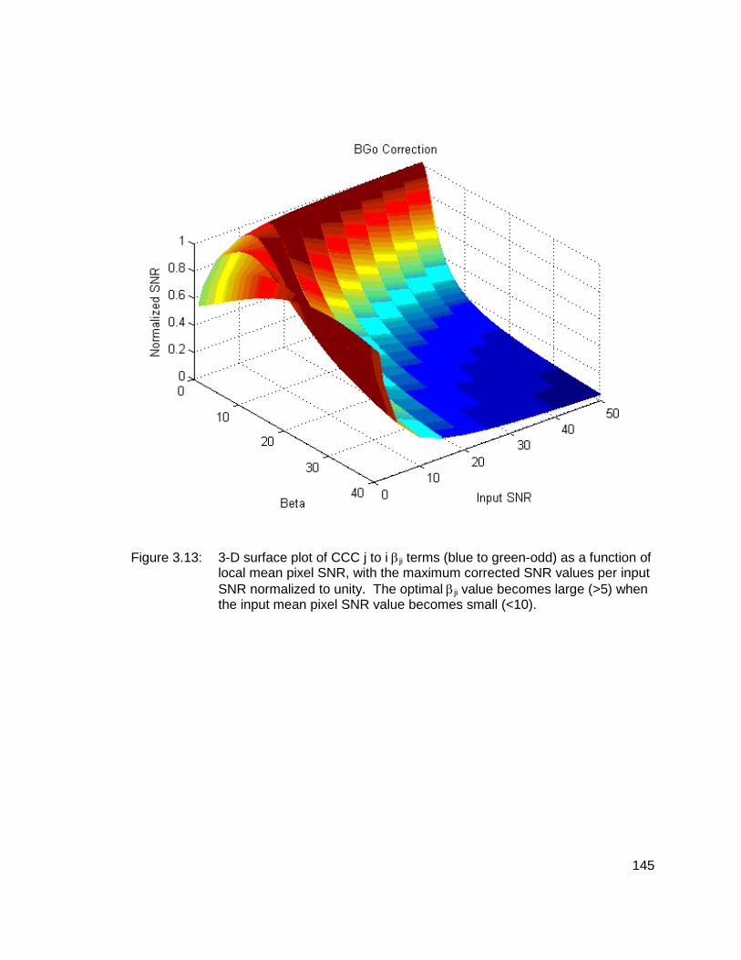
145

Figure 3.13: 3-D surface plot of CCC j to i βji terms (blue to green-odd) as a function of local mean pixel SNR, with the maximum corrected SNR values per input SNR normalized to unity. The optimal βji value becomes large (>5) when the input mean pixel SNR value becomes small (<10).

146

Figure 3.14: CCC i to i βii terms (green-odd to green-odd) as a function of local pixel SNR, with the maximum corrected SNR values per input mean SNR normalized to unity. There is a dark red (maximum corrected SNR) region close to the left edge of the plot (at β<0.01). On-diagonal blurring filters are better conditioned, requiring smaller optimal βii terms. The optimal βii value remains small (<0.1) even when the input mean pixel SNR value is small (<10), and the optimal βii value is very small (<0.001) when the input SNR is in its normal operating range (>10).

147

Figure 3.15: 3-D surface plot of CCC i to i βii terms (green-odd to green-odd) as a function of local pixel SNR, with the maximum corrected SNR values per input SNR normalized to unity. The optimal βii value remains small (<0.1) even when the input mean pixel SNR value is small (<10), and the optimal βii value is very small (<0.001) when the input SNR is in its normal operating range (>10).

The test image used in our analysis is shown in Figure 3.16. This test image possesses

all of the features that concern us: saturated colors, low and high spatial frequency data.

The range of input mean SNR values was obtained by adjusting input lighting values and

exposure times. Additionally, ideal images were created by utilizing multiple frame

averaging to remove temporal noise and full fixed pattern noise removal along with ideal

cross-talk inversion (with near zero noise).

148

Figure 3.16: Ideal input test image used for performance analysis.

The cross-talk and noise corruption of the ideal input test image has a detailed section

shown in Figure 3.17 for an overall input SNR of 30, which corresponds to an electron to

digital count conversion factor (e-/DN) of 1.4. In Figure 3.18, we show samples of an

image cross-talk corrected by the simple 3x3 matrix color correction method, the ST

method, and our SCLS SNR method. These images show the overall corrected SNR

value and the SNR value of the gray square (18% gray). The overall SNR is our metric

that we use to measure image correction. It is the average corrected pixel SNR, using

the knowledge of the ideal (uncorrupted) pixel values. The 18% gray SNR is the

measured flat field SNR of the MacBeth chart 18% reflector gray square. It is a metric

commonly used in industry to measure the quality of processed sensor images (refer to

149

ISO standard 12232-1998E). The three images show that the SCLS SNR method

performs better than the other two methods of similar complexity. It should be noted that

further processing would typically be performed on the cross-talk restored pixel data.

One can view the cross-talk restoration process as the color correction step in the color

sensor process (along with the Bayer interpolation step). After the color correction step,

one might perform some sort of flat area noise smoothing (such as median filtering) and

an edge sharpening filtering. These image processing steps would improve the

appearance of the final processed images.

Figure 3.17: Input test image detail section corrupted for conversion factor e-/DN=1.4, Overall SNR=30, 18% Gray SNR=18. Images with any specified SNR value can be constructed using characterization and camera system models.

150

Figure 3.18: Detail of SNR=30 image section after correction by methods:

Top Left: Optimal 3x3 Matrix, Overall SNR=35, 18% Gray SNR=15, Top Right: ST, Overall SNR=37, 18% Gray SNR=16, Bottom: SCLS SNR, Overall SNR=42, 18% Gray SNR=18.

3.5.2 Discussion of Performance and Conclusions

The separate optimization of CCC terms has been shown to be very advantageous for

the Bayer cross-talk problem. This is due to the full restoration of within color channel

blurring (j=i) usually having small noise amplification (small blur matrix condition

number), whereas the full restoration of cross color channel blurring (j≠i) often having

151

large noise amplification (large blur matrix condition number). Although methods such

as [27] can scale the Q matrices for different CCCs, they cannot simultaneously adjust

for the CCC’s blurring matrix stabilities and SNR values.

The pixel SNR after correction for within color channel blurring (j=i) is more sensitive to

bias error, than the pixel SNR for cross color channel blurring (j≠i). This is due to the

majority of the correction for the within color channel blurring case being a simple

gaining of the target pixel’s value. Because of this, the pixel signal divided by pixel noise

ratio will have little change as the regularization parameter’s value approaches zero.

This is also a consequence of the within color channel blurring filters having smaller

condition numbers. However, the bias error will increase as regularization parameter’s

value increases. Correcting the within color channel blurring corresponds to a heuristic

white balance correction in a standard camera system, which does not affect the SNR

due to the noise variance. Thus, to maximize the pixel SNR due to noise variance and

bias error (total noise), a correction approaching the ideal full inverse correction (βii=0) is

usually required. Since, from a HVS standpoint, the white balance should always be

performed, the proposed restoration method’s behavior matches the HVS’s sensitivities

[64], [75], [76], [85]. Existing methods that use the MSE as a metric for calculating the

regularization parameter will not produce the optimal value for white balance, since the

noise variance will increase with a decreasing regularization parameter value. Even

when the bias error is included in the MSE calculation, this will result in too large of a

regularization parameter value being calculated.

For the cross color channel blurring (j≠i) case, more independent pixels in the local

neighborhood are involved in the correction, leading to a noise amplification situation.

152

This is a consequence of the cross color channel blurring filters having larger condition

numbers. The CCC correction will involve between 4 and 6 pixels in the local 5 by 5

pixel neighborhood. Thus, more blurring, resulting from a greater regularization

parameter value (βji>0), is often required in order to obtain the maximum corrected pixel

SNR. The optimal value of βji will result from the maximum value of the corrected CCC

divided by the total MSE derived as the sum of the corrected noise variance and the

corrected bias error. Existing methods that do not take into account bias error will

produce regularization parameters that are too large and penalize the saturation

correction too much. Additionally, even existing methods that use the total MSE

estimate for the regularization calculation do not consider the estimated corrected SNR

value. The HVS’s sensitivity to the local SNR relationship is not represented well by the

MSE. Methods using the MSE metric will find minimum MSE regularization parameter

values which attenuate the corrected signal value too much. As a result, from the

maximum SNR point of view, they will produce regularization parameters that are too

large and overly reduce the saturation correction. From the HVS’s sensitivity to local

SNR [7], [19], [56], [73], the existing methods using the MSE metric will over smooth the

images.

Using our proposed method for a local pixel area with a high SNR for all of the color

components, we will apply an ideal inverse filtering correction. This corresponds to an

ideal full 3x3 color correction TCC matrix application in a heuristic camera system, which

corrects white balance and saturation. When we have a local pixel area with a low SNR

for all of the color components, we will apply close to an ideal inverse filtering correction

for the within CCC terms, but a greatly regularized correction to the cross CCC terms.

This is similar to a heuristic camera system applying an ideal white balance correction

153

TWB matrix with a greatly reduced TSat matrix. This separate optimized correction of the

CCCs is not possible in the existing methods that use one regularization parameter per

channel.

The greatest visual effect of Bayer cross-talk blurring is the de-saturation of color. Since

the extent of the blurring is often limited to a local 5 by 5 pixel neighborhood, blurring of

the high frequency details of the image will not be as noticeable to the human observer

as is the color corruption. Since the Bayer color filter array has different color filtered

(CFA) pixels next to one another, there will be significant color blurring for small pixels.

Thus, the trade-off between color correction and noise amplification will be the most

significant criterion. This criterion leads us to use the local mean SNR estimate as the

metric in selecting the optimal regularization parameter. Since the HVS sensitivity to

color is greatest for low frequency components [64], [75] (Figure 3.7), the local mean

values are best to use in the correction process. As discussed in this thesis, the HVS is

also sensitive to relative error or local SNR. Thus, the use of the local average SNR is

best to use in the correction of local pixel values and consequently the local color values.

In summary, the advantages of our proposed SCLS SNR method over standard camera

correction methods being used are that our method:

1) is spatially adaptive

2) treats each CCC separately and optimally

3) corrects the green odd and even channels (which have different cross-talk characteristics)

4) uses sensor characterization models which define pixel SNR values as a function of pixel signal level

5) is automatically matched to the HVS’s SNR sensitivity

6) can be implemented as a simple, direct method

154

3.5.3 Comparison to Red/Black Ordering

One of the key assumptions and simplifications that we make in our SCLS SNR method

is that each CCC is independent from each other. This assumption will not usually be

valid, since each color channel is typically not independent from the other color

channels. The amount of correlation between color channels changes as a function of

spatial location within a picture. The color channel correlation also varies greatly from

picture to picture. The greatest correlation between color channels will be between the

odd and even green channels of a Bayer CFA imager. This is where the breakdown of

the channel independence assumption will be the most severe.

A multigrid method, such as Red-Black Gauss-Seidel, can be used to parallelize

computations. In these schemes, a set of points (red points) are updated at one step,

and then another set of points (black points) are updated in the next step. For an image,

this would be done on a single channel. The two-color (red/black) approach using a 5-

point Laplacian can be used to separate the coupling between any two points (red or

black points), so that any point can be updated simultaneously. In our application, we

assume each plane is independent. Thus, we are not applying a red/black type sub-

sampling of a color plane. One important feature of our method is that it is not iterative.

Red/black-ordering uses a successive over-relaxation (SOR) type iterative solution,

which would not be applicable to our Bayer cross-talk problem due its constraints.

155

Chapter 4

Conclusions and Future Work

4.1 Conclusions

Sensor characterization data and camera system image processing information

were utilized to develop image sensor testing and image quality enhancement

methods for commercial CMOS image sensors. The approach we developed

was to link system algorithms to the sensor performance characteristics.

In Chapter 2, we presented novel image sensor PRNU testing methods. Monte

Carlo and probability model-based simulation approaches were used to create

functions which relate measurements of raw block PRNU values to failure rates

for particular sensor applications. These methods allow failure rate curves to be

constructed for specific sensor operating conditions and image processing

settings. Groups of settings can be associated with specific sensor applications.

In the development of our methods, we used the idea that different sensor

applications will have different requirements for quantization (compression)

amounts, acceptable SNR, image processing applied, sensor gain settings,

sensor exposure times, and other operating conditions. We also used the

concept of acceptable degradation to determine sensor operation based PRNU

thresholds. Sensor signal-dependent noise models were used in the process of

156

determining these thresholds. Using our proposed PRNU testing methodologies,

we have shown the potential to increase the yield rate of sensors. A single

PRNU measurement per sensor can be used for multiple sensor applications,

which increases testing efficiency and reduces overhead cost.

A novel, low complexity pixel cross-talk correction algorithm that can provide

restoration performance better than heuristic methods currently implemented in

low cost camera systems, was developed in Chapter 3. The use of separate

color channel component (CCC) restoration based on local pixel SNR information

was primarily responsible for the excellent performance of our CCC separated

constrained least squares (SCLS) with local SNR optimization constraint

regularization method (SCLS SNR). The optimal value of each CCC

regularization parameter was determined to be a function of the CCC blurring

filters and the local pixel CCC SNR value. Since there is a wide range in the

different CCC blurring filter stability (ill-condition-ness) and in the spatial color

channels SNR, the use of this optimization of the local CCC regularization

parameter is both appropriate and beneficial. It was shown that the

regularization parameter values for each CCC, as a function of local pixel SNR,

can be calculated and stored in a LUT. Additionally, the corresponding

coefficients for the SCLS SNR convolution filters can be calculated off-line and

stored for real-time use in a camera system. This approach minimizes the

required number of calculations that must be performed in a camera system

during image processing. Cross-talk and signal-dependent noise models,

determined from sensor characterization, were utilized in the development of our

SCLS SNR method.

157

4.2 Future Work

4.2.1 PRNU

In order to acquire a better understanding of the applicability of our PRNU testing

method, error thresholds and error rates need to be determined for a larger set of

sensor applications. A greater set of application requirements, such as data

rates (which determine amount of compression), need to be determined and

used in the PRNU analysis. Allowable error rates for the greater set of sensor

applications should also be found and used in the PRNU distortion analysis. We

need more data on the acceptable PRNU block failure rates per sensor. One

problem with this is that much of the information is company proprietary. Most

importantly, we need to determine quantitatively the yield rate improvement that

one could achieve by using our PRNU testing approach.

We may also want to look at the failure rates for particular PRNU block patterns.

The spatial distribution of pixel gain factors within a block will determine the

spatial frequency PRNU characteristics. This will in turn have an affect on the

perceptual distortion of the block image data. Thus, instead of simply measuring

a standard deviation or maximum/minimum difference of PRNU, we could also

consider the spatial locations of pixel gain variation. During testing, pixel blocks

could be grouped into PRNU distribution 'classes', with the allowable distortion

based upon the block PRNU class.

4.2.2 Bayer Cross-Talk Correction

The weakened optimization used in our SCLS SNR algorithm requires further

analysis. The error resulting from neglecting the correlation between different

158

CCC components is image dependent, and should be quantified for a

representative set of input images to a camera system.

The SCLS SNR algorithm could be combined with the color correction frequency

domain method that was developed in [61]. We could extend the SCLS SNR

method to be applied within the frequency domain. The algorithm could be

applied to individual subbands obtained from a discrete wavelet transform

(DWT), or to frequency coefficients from the discrete cosine transform (DCT).

This correction method could then be embedded in the compression operations

of JPEG or JPEG 2000.

The DCT domain can be used to segment the image frequency components for

each sensor color plane. At the same time, we can implement the cross-talk and

color correction into the JPEG compression process, similar to the method of

Chapter 3. As shown in Figure 4.1, the white balanced (scaled) raw Bayer data

for the four-color planes would have the DCT applied to them. For each color

plane (R, Ge, Go, B) and each DCT coefficient, in the absence of noise, there

exists a set of inverse blurring coefficients that can be applied to best recover the

corresponding component of color plane coefficients. The DCT coefficient

correction is shown in Figure 4.2. The Cijk coefficients are the optimal inverse

blurring coefficients for coefficient i spatial frequency and CCC j to k correction.

A method to derive these coefficients from the ideal spatial domain filters would

have to be developed. In the presence of noise, we would have to adjust the

blurring and color corrections. We could accomplish this by using the scalar

terms Kijk SNR shown in Figure 4.2. The JPEG compression process can then

continue from this point in the standard manner.

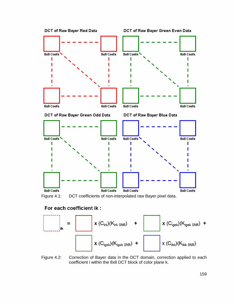
159

Figure 4.1: DCT coefficients of non-interpolated raw Bayer pixel data.

Figure 4.2: Correction of Bayer data in the DCT domain, correction applied to each

coefficient i within the 8x8 DCT block of color plane k.

160

Bibliography

[1] S. Agwani, S. Domer, et al, “High Performance VGA Resolution Digital Color CMOS Imager”, Proc. SPIE Vol. 3649, pp. 154-164, Sensors, Cameras, and Systems for Scientific/Industrial Applications, Apr. 1999.

[2] J.M.M. Anderson, B.A. Mair, M. Rao, C.-H. Wu, “Weighted Least-Squares Reconstruction Methods for Positron Emission Tomography”, IEEE Trans. Med. Imaging 16(2): 159-165, 1997.

[3] H. Andrews and B. Hunt, Digital Image Restoration, Englewood Cliffs, NJ: Prentice Hall, 1977.

[4] M. Antonini, M. Barlaud, P. Mathieu, L. Daubechies, “Image Coding Using Wavelet Transform”, IEEE Transactions on Image Processing, vol: 1 Issue: 2, pgs. 205 –220, Apr. 1992.

[5] M.R. Banham and A.K. Katsaggelos, “Digital Image Restoration”, IEEE Signal Processing Magazine, pgs 24-41, March 1997.

[6] Y. Bao, and Y. Noyes, “Dorado2 Image Processing Algorithms and System Specifications”, I.C. Processor Spec., Pictos Technologies, Inc, 2003.

[7] P.G.J. Barten, “Contrast Sensitivity of the Human Eye and Its Effects on Image Quality”, SPIE Publications, Vol. PM72, Dec 1999.

[8] B. Benwell, N. O., G. Allen, et Al., “12k 5-mm linescan CCD sensor with 320 MHz data rate”, 2005 IEEE Workshop. on Charge-Coupled Devices and Advanced. Image Sensors, June 10-12, 2005.

[9] A.J. Blanksby and M.J. Loinaz, “Performance Analysis of a Color CMOS Photogate Image Sensor”, IEEE Trans on Electron Devices, Vol 47, Issue 1, pp. 55-64, Jan 2000.

[10] J.T. Buey, “First Results on the Corot CCD Test Bench”, The Third MONS Workshop: Science Preparation and Target Selection, January 24-26, 2000.

[11] Y. Chen, S.M. Guertin, et Al., “A Chip and Pixel Qualification Methodology on Imaging Sensors”, IEEE Reliability Physics Symposium Proc., 42nd Annual, pp435- 439, April 2004.

161

[12] I.S. Chong, and A. Ortega, “Hardware Testing for Error Tolerant Multimedia compression base on Linear Transforms”, DFT 2005, IEEE, pp. 523 - 531, 3-5 Oct. 2005.

[13] I.S. Chong, H.Y. Cheong, and A. Ortega, “New Quality Metrics for Multimedia Compression Using Faulty Hardware”, Proc. Video Processing and Quality Metrics for Consumer Electronics (VPQM'06), Jan. 2006.

[14] J. Chou, M. Crouse, and M. K. Ramchandran, “A Simple Algorithm for Removing Blocking Artifacts in Block-Transform Coded Images”, IEEE Signal Processing Letters, vol: 5 Issue: 2, pgs. 33–35, Feb. 1998.

[15] Conexant CX1024 Sensor Design and Manufacturing document, A. Dumas, B.C. Hseih, J. Luo, R. Mann.

[16] Conexant CX20450 (SXGA) Sensor Electra-Optical Specification document, S. Bencuya, F. Gunawan, B.C. Hseih, R. Mann, B. McCleary.

[17] Conexant DVGA 20490 Rev A, Sensor Characterization Test Report, R. Kannegundla, R. Mann, B. McCleary.

[18] Conexant DVGA 20490 Sensor Electra-Optical Specification document, S. Bencuya, R. Kannegundla, R. Mann, B. McCleary, E. Stauber.

[19] W.J. Crozier, “On the variability of critical illumination for flicker fusion and intensity discrimination”, Journal of General Physiology, Vol. 19, pp. 503-522, 1935.

[20] A. El Gamal and H. Eltoukhy, “CMOS image sensors”, IEEE, Circuits and Devices Magazine, Vol 21, Issue 3, pp. 6-20, May-June 2005.

[21] Fairchild Imaging, CMOS 1421 Specification Sheet, Rev C, Table 9, 2005.

[22] J.A. Fessler, “Mean and Variance of Implicitly Defined Biased Estimators (such as Penalized Maximum Likelihood): Applications to Tomography”, IEEE Conf. Acoustic Speech Sig. Proc., vol. 4, pp. 2291-2294, 1995.

[23] J.A. Fessler, “Penalized weighted least-squares image reconstruction for positron emission tomography”, IEEE Trans. Med. Imag., 13(2):290-300, Jun. 1994.

[24] J.A. Fessler, W.L. Rogers, “Spatial Resolution Properties of Penalized-Likelihood Image Reconstruction: Space-Invariant Tomographs”, IEEE Transactions on Image Processing , Vol. 5, Issue 9, pp. 1346-1358, 1996.

[25] N.P. Galatsanos and R.T. Chin, “Restoration of Color Images by Multichannel Kalman Filtering”, IEEE Transactions on Signal Processing, Vol. 39, No. 10, Oct 1991.

162

[26] N.P. Galatsanos, A.K. Katsaggelos, “Methods for Choosing the Regularization Parameter and Estimating the Noise Variance in Image Restoration and Their Relation”, IEEE Transactions on Image Processing, Vol. 1, No. 3, pp. 322-336, July 1992.

[27] N.P. Galatsanos, A.K. Katsaggelos, R.T. Chin, A. Hillery, "Least Squares Restoration of Multi-Channel Images,'' IEEE Trans. Signal Processing, vol. 39, no. 10, pp. 2222-2236, Oct. 1991.

[28] N.P. Galatsanos, R.T. Chin, “Digital restoration of multichannel images”, IEEE Trans. on Acoustic, Speech and Signal Proc., Vol. 37, No. 3, pp. 415-421, March 1989.

[29] N.P. Galatsanos, R.T. Chin, A.K. Katsaggelos, A. Hillery "Two Methods for Least Squares Multi-Channel Image Restoration,'' IEEE International Conference on Acoustics, Speech, and Signal Processing, ICASSP-91, Vol.4, pp. 2509-2512, Apr 1991.

[30] D. Gardner, “Taking a Closer Look at Camera Specifications”, Phontoics Spectra, May 2003.

[31] R.C. Gonzales and R.E. Woods, Digital Image Processing, chapter 5, Addison-Wesley Publishing Co., Reading, MA, Sept 1993.

[32] W. Hardin, "CMOS Sensors Offer Vision Designers New Capabilities", Machine Vision Online, April 2004.

[33] B. Hochfelder, “Looking at the Expanding Sensor Market”, Advanced Imaging, May 2008.

[34] A.E. Hoerl and R.W. Kennard, “Ridge regression: Biased estimation for nonorthogonal problems,” Technometrics, vol. 12, no. 1, pp.55-67, 1970.

[35] G.C. Holst “CCD Arrays Cameras and Displays”, SPIE Optical Engineering Press, Bellingham, WA, 2nd edition, 1998.

[36] M.C. Hong, T. Stathakiet, A.K. Katsaggelos, “A Regularized Mixed Norm Multichannel Image Restoration Approach,” Statistical Signal and Array Processing, Ninth IEEE SP Workshop, Sept 1998.

[37] B. Hunt, H. Trussell, “Sectioning techniques for processing signals with signal-dependent noise”, Acoustics, Speech, and Signal Processing, IEEE International Conference on ICASSP, Vol 2, 704- 707May 1977.

[38] H.T. Hytti, “Characterization of digital image noise properties based on RAW data”, Proc. of SPIE and IS&T, vol. 6059, Jan. 2005.

[39] B. Jahne, and H. Haussecker, “Computer Vision and Applications: A Guide for Students and Practitioners ”, Academic Press; May 15, 2000.

163

[40] J. Janesick, “Dueling Detectors”, SPIE’s oemagazine, Feb. 2002.

[41] J. Janesick, “Lux transfer: Complementary metal oxide semiconductors versus charge-coupled devices,” SPIE, Opt. Eng. 41, pp. 1203-1215, June 2002.

[42] J. Janesick, Scientific Charge-Coupled Devices, chapter 2, SPIE Press, Bellingham, Washington, vol. PM83, 2001.

[43] H.R. Kang, “Color Technology for Electronic Imaging Devices”, chapters 2 & 3, SPIE Optical Engineering Press, Bellingham, Washington, Jan. 1997.

[44] M.G. Kang , “Generalized multichannel image deconvolution approach and its applications”, Optical Engineering, Vol. 37, No. 11, pgs 2953-2964, Nov 1998.

[45] M.G. Kang and A. K. Katsaggelos, "General Choice of the Regularization Functional in Regularized Image Restoration,'' IEEE Trans. Image Processing, Vol. 4, No. 5, pp. 594-602, May 1995.

[46] N.B. Karayiannis, A. N. Venetsanopoulos, “Regularization theory in image restoration--the stabilizing functional approach”, IEEE Transactions on Acoustics, Speech, and Signal Processing, Vol. 38, No. 7, pp.1155-1179, July 1990.

[47] A.K. Katsaggelos, “A General Formulation of Adaptive Iterative Image Restoration Algorithms,” Proc. 1986 Conf. Inf. Sciences and Systems, pp. 42-47, March 1986.

[48] A.K. Katsaggelos, J. Biemond, R.W. Schafer, R.M. Mersereau, “A Regularized Iterative Image Restoration Algorithm”, IEEE Transactions on Signal Processing, Vol. 39, No. 4, pgs 914-929, April 1991.

[49] D.T. Kuan, A.A. Sawchuk, T.C. Strand, P. Chavel, “Adaptive noise smoothing filter for images with signal-dependent noise”, IEEE Trans. Pattern Anal. Machine Intell., vol. PAMI-7, no. 2, pgs. 165–177, March 1985.

[50] D.T. Kuan, A.A. Sawchuk, T.C. Strand, P. Chavel, “Nonstationary 2-D Recursive Restoration of Images with Signal-Dependent Noise”, IEEE International Conf on Acoustics, Speech and Signal Processing ICASSP, Vol. 9, pp. 84- 87, Mar 1984.

[51] M.L. La Haye, C. Jung, et al., “Fault Tolerant Active Pixel Sensors in 0.18 and 0.35 Micron Technologies”, IEEE, Defect and Fault-Tolerance in VLSI Systems, 2006.

[52] F.M. Li, and Arokia Nathan, “CCD Image Sensors in Deep-ultraviolet”, Springer Berlin Heidelberg, 2005.

[53] Q. Li, E. Asma, J. Qi, J.R. Bading, RM. Leahy, “Accurate estimation of the Fisher information matrix for the PET image reconstruction problem”, IEEE Trans Med Imaging, Vol. 23, No. 9, pp.1057-1064, Sept 2004.

164

[54] W. Li, P. Ogunbona, Y. Su, I. Kharitonenko, “Modelling of Color Cross-Talk in CMOS Image Sensors”, IEEE International Conference on Acoustics, Speech, and Signal Processing, Vol 4, pgs 3576-3579, May 2002.

[55] C.M. Lo, A.A Sawchuk, “Nonlinear restoration of filtered images with Poisson noise”, Society of Photo-Optical Instrumentation Engineers, p. 84-91, August 1979.

[56] L.N.D. Loo, K. Doi, C.E. Metz, “A comparison of physical image quality indices and observer performance in the radiographic detection of nylon beads”, Physics in Medicine and Biology, Vol. 29, No. 7, pp. 837-856, July 1984.

[57] B. McCleary, “A scalar quantization method for noisy CMOS imager data”, Proc. of the SPIE, Vol. 5208, pp. 153-164, 2004.

[58] B. McCleary, “Color Correction Methods to Reduce Pixel Random Noise for CX20450", Conexant internal memo, Aug. 2000.

[59] B. McCleary, “Cross-talk adjustment in electronic imaging devices”, United States Patent 7170555, Issued Jan. 2007.

[60] B. McCleary, “Cross-talk correction methodology for color CMOS imagers,” Proc. IS&T/SPIE International Symposium on Electronic Imaging, SPIE Vol. 5678, pp. 117-128, Jan. 2005.

[61] B. McCleary, “Methods to Reduce the Amplification of Random Noise in the Color Processing of Imager Data”, IS&T's 2003 PICS Proceedings, pp. 50-57, Jan. 2003.

[62] R. Molina, J. Mateos, A.K. Katsaggelos, M. Vega, “A General Multichannel Image Restoration Method Using Compound Models” IEEE Computer Society, Proceedings of the 16th International Conference on Pattern Recognition, ICPR, Vol. 3, pp. 30835, 2002.

[63] R. Molina, J. Mateos, A.K. Katsaggelos, M. Vega, “Bayesian Multichannel Image Restoration Using Compound Gauss-Markov Random Fields”, IEEE Transactions on Image Processing, Vol. 12, No. 12, Dec 2003.

[64] K. Mullen, “The contrast sensitivity of human color vision to red-green and blue-yellow chromatic gratings,” Journal of Physiology, vol. 359, pp. 381-400, 1985.

[65] B. Natarajan, “Filtering Random Noise from Deterministic Signals via Data Compression”, IEEE Transactions on Signal Proc., 43(11), Nov. 1995.

[66] S. Oraintara, W. C. Karl, D. A. Castañon, T. Q. Nguyen, “A Method for Choosing the Regularization Parameter in Generalized Tikhonov Regularized Linear Inverse Problems”, ICIP 2000.

165

[67] M.K. Özkan, A.T. Erdem, M.I. Sezan, A.M. Tekalp, "Efficient Multiframe Wiener Restoration of Blurred and Noisy Images Sequencyes,'' IEEE Transactions on Image Processing, Vol. 1, No. 4, pp. 453-476, Oct 1992.

[68] B. Pain, B. Hancock, “Accurate Estimation of Conversion Gain and Quantum Efficiency in CMOS Imagers,” Proceedings of SPIE-IS&T Electronic Imaging, SPIE vol. 5017, pp. 94-103, 2003.

[69] B. Pain, G. Yang, B. Olson, et al., “A low-power digital camera-on-a-chip implemented in CMOS active pixel approach,” Proceedings of VLSI Design, pp. 26-31, Jan. 1999.

[70] W.B. Pennebaker, and J.L. Mitchell, “JPEG Still Image Data Compression Standard,” Chapman & Hall, New York, 1993.

[71] J. Qi, R.M. Leahy, “A Theoretical Study of the Contrast Recovery and Variance of MAP Reconstructions from PET Data”, IEEE Trans. on Medical Imaging, vol. 189, no. 4, pp. 293-305, April 1999.

[72] M.A. Robertson, and R.L. Stevenson, “DCT Quantization Noise in Compressed Images”, IEEE Trans, Vol. 15, Issue 1, pp 27-38, Jan. 2005.

[73] A. Rose, “The sensitivity performance of the human eye on an absolute scale”, Journal of the Optical Society of America, Vol. 38, pp. 196-208, 1948.

[74] K. Sauer and C. Bouman, “A Local Update Strategy for Iterative Reconstruction from Projections”, IEEE Trans. on Sig. Proc., vol. 41, no. 2, pp. 534-548, Feb. 1993.

[75] O.H. Schade, “On the quality of color-television images and the perception of colour detail,” Journal of the Society of Motion Pictures and Television Engineers, vol. 67, no. 12, pp. 801–819, 1958.

[76] O.H. Schade, “Optical and photoelectric analog of the eye,” Journal of the Optical Society of America, vol. 46, no. 9, pp. 721–739, 1956.

[77] M. Sezan, A. Tekalp, C-T. Chen, “Regularized signal restoration using the theory of convex projections”, Acoustics, Speech, and Signal Processing, IEEE International Conference on ICASSP, Vol. 12, pp. 1565-1568, Apr 1987.

[78] J.H. Shin, J.K Paik, M.G. Kang, "Comparison between Wiener and CLS Image Restoration Techniques for Multichannel Images,'' Proceedings of IEEE Asia Pacific Conf on Circuits and Systems, pp. 532-535, Nov 1996.

[79] J.W. Stayman., J.A. Fessler, “Regularization for uniform spatial resolution properties in penalized-likelihood image reconstruction”, IEEE Trans Med Imaging.;19(6):601-15., June 2000.

166

[80] Y.P. Tan and T. Acharya, “A Method for Color Correction with Noise Consideration”, IS&T/SPIE, vol. 3963, pgs. 329-337, Jan. 2000.

[81] A.A. Tanbakuchi, A. van der Sijde, B. Dillen, A. Theuwissen, and W. de Haan, “Adaptive pixel defect correction”, Proc. of SPIE-IS&T, SPIE vol. 5017, 2003

[82] A.N. Tikhonov and V.Y. Arsenin, Solutions of Ill-Posed Problems, chapters 1 & 2, V.H. Winston & Sons, Washington D.C., 1977.

[83] F. Truchetet, B. Joanne, F. Perot, and O. Laligant, “High-Quality Still Color Image Compression”, Optical Engineering/SPIE, Vol. 39(02), pgs.409-414, Feb. 2000.

[84] H.J. Trussel and R.E. Hartwig , “Mathematics for Demosaicking”, IEEE Transactions on Image Processing, Vol 11, No. 4, pgs 485-492, April 2002.

[85] B.A. Wandel and X.M. Zhang, “A spatial extension to CIELAB for digital color image reproduction,” Society for Information Display Symposium Technical Digest, vol. 27, pp. 731-734, 1996.

[86] X.W. Wang, C. Wang, "Regularized Image Restoration Based on Adaptively Selecting Parameter and Operator,'' Processings of the 17th International Conference on Pattern Recogniton, IEEE, Vol 3, Issue 23-26, pp. 662-665, Aug. 2004.

[87] A.B. Watson, “Visual detection of spatial contrast patterns: Evaluation of five simple models”, Optics Express, Vol. 6, Issue 1, pp. 12-33, Jan. 2000.

[88] A.B. Watson, and A.J.J. Ahumada, “An improved detection model for DCT coefficient quantization”, SPIE Proc. 1913, pp 191-201, 1993.

[89] A.B. Watson, and R. Rosenholtz, “Perceptual adaptive jpeg coding”, Vol. 1, pp. 901-904, 16-19 Sep 1996.

[90] A.B. Watson, J. Hu, and J.F. McGowan, “Digital video quality metric based on human vision”, SPIE, Journal of Electronic Imaging, vol. 10, pp 20-29, Jan 2001.

[91] S. Welstead, “Fractal and Wavelet Image Compression Techniques”, SPIE Press, vol. TT40, pgs. 131-153, Nov. 1999.

[92] T. Zarnowski, T. Vogelsong, and J. Zarnowski, “Inexpensive Image Sensors Challenge CCD Supremacy”, Photonics Spectra, pgs. 188-190, May 2000.

[93] W. Zhu, N. P. Galatsanos and A. K. Katsaggelos, "Regularized Multi-Channel Image Restoration Using Cross-Validation'', Proc. SPIE Conf. on Visual Communications and Image Processing, SPIE Vol. 1818, pp. 345-356, Nov. 1992.

167

Appendix A

CMOS Imager Noise

CMOS image sensors experience noise from numerous noise sources. The resulting

aggregate noise has both time-invariant (fixed-pattern) and time-variant (temporal)

behavior. The use of the term fixed-pattern noise refers to any spatial pattern that does

not change significantly from frame to frame, whereas, the temporal noise changes from

frame to frame [42]. A noise transfer diagram is shown in Figure A.1 for a typical CMOS

imager [35]. The temporal (time variant) noise that CMOS sensors encounter includes

[92]: photon shot noise, capacitive reset (kTC) noise, dark current time-varying noise,

Johnson (thermal or white) noise, and 1/f noise (frequency-dependent). Additionally,

CMOS imagers can suffer significant temporal noise from electrical ground-bounce and

coupling noise problems generated by on-chip logic and ADC circuitry. Fixed pattern

noise (FPN) is generated in CMOS imagers by pixel variations in dark current and

sensitivity, as well as pixel fixed offset. It is common practice to express the values of

the noise sources in root mean square (RMS) electron values.

Photon shot noise is created by the uncertainty due to the quantum nature of light [42].

The measurement process can be considered a Poisson counting process, since the

168

sensor is in effect counting the arrival of photons. The probability that n photons will

arrive at a pixel during a time interval T with a photon flux (photon event rate) of r is

given by the probability mass function:

p(n | r) = ( ) e T

!T rn

nr − (A.1)

If the number of photons detected by the device is large, then the noise can be well

modeled by a signal-dependent Gaussian distribution [42]. Since the underlying process

is Poisson, the variance of the Gaussian approximation is equal to the mean. This

relationship is very useful in the characterization of image sensors. Each pixel can be

treated as independent from the others. When photon shot noise is much greater than

other sources of noise, then we say that the sensor is shot noise limited [42]. The

signal-to-noise ratio (SNR) can be then determined using only photon shot noise. The

maximum number of electrons that a pixel can hold is called the full well of the pixel [42].

Sensors that have larger full well will have a larger maximum signal to noise ratio when

they are shot noise limited. Smaller pixels have a smaller maximum signal to shot noise

ratio [41]. These effects reduce the sensor’s dynamic range and SNR for small pixels.

Dark current is signal that is generated by the sensor independent of incoming light

signal [42]. Dark current has three main sources of generation. The first is thermal

generation in the depletion region of the photodiode. The second is thermal generation

and diffusion in the bulk material of the sensor. Lastly, dark current is created by surface

states. Dark current can result in both temporal and fixed pattern noise [42]. The

temporal dark current is dark current shot noise. If the number of electrons generated by

dark current is large, then the dark current temporal noise can be modeled as a dark

169

current signal-dependent Gaussian distribution. Variation from pixel to pixel in the

amount of dark current generation results in pixel-to-pixel fixed pattern noise. The dark

current is a function of temperature, roughly doubling for every 8°C increase [42]. It is

also directly proportional to the integration time. At higher temperatures and longer

exposure times, the dark current fixed pattern noise can become a dominant noise

source, limiting the SNR of an image. The fixed pattern dark current, or pixel-to-pixel

mean dark current, can be subtracted out from an image frame. However, the temporal

component, dark current shot noise, cannot be removed in this simple manner.

Scientific imagers can be cooled to significantly reduce dark current. However,

commercial consumer imagers usually do not have this option, especially embedded

imaging sensors. Thus, due to dark current concerns as well as motion blur, the

maximum exposure or integration time for an embedded application sensor is limited,

typically to no more than 30 to 60 ms.

One of the dominant sources of temporal noise in CMOS imagers is pixel reset noise

[92], which occurs when the sense node capacitor of the pixel is reset using the reset

transistor. Refer to Figure A.2 for a typical 3T transistor, which has reset, source

follower, and row select transistors. This noise is generally uncorrelated from pixel to

pixel [40], [42]. The reset field-effect transistor switch generates the kTC noise, where k

is Boltzmann’s constant, T is the temperature, and C is the capacitance of the attached

load. The kTC reset noise is due to the thermal noise generated by the resistance within

the reset transistor [42]. After the photodiode is reset, the capacitance of the floating

diffusion is recharged through the noisy reset transistor. As the size of the pixel

photodiode is reduced due to the demands of embedded applications, the capacitance

also decreases. This increases the kTC noise, as well as decreasing the full-well signal

170

level. A passive pixel sensor (PPS) uses a MOS transistor acting as a switch to connect

to the column circuitry. This pixel architecture is limited in performance due to the small

capacitance of the photodiode connected to the large column circuitry readout

capacitance. Adding a small amplifier (source follower) to every pixel results in the

active pixel sensor (APS) architecture. Compared to the PPS, the APS reduces the

pixel reset noise, as well as fixed pattern noise. The imagers used in this document are

all APS CMOS sensors. Reset noise for CMOS imagers usually falls in the range of 20

to 70 noise electrons, depending on the pixel architecture and the sense node sensitivity

(V/e-) [40]. The value of the reset noise can be determined from the Johnson noise

current variance:

σi2 = (4kT/R) ∆f , (A.2)

where ∆f is the noise equivalent bandwidth and is given by ∆f = RC/4, with C the sense

noise capacitance. Then we have:

σi2 = kTC (A.3)

The root mean squared (rms) noise in electrons is then:

σe = q

kTC , (A.4)

where q is the electronic charge, and Equation (A.4) gives the uncertainty in the amount

of charge in the capacitor after it has been reset. When uncorrelated double sampling is

used, as with a 3T pixel design, then two uncorrelated pixel resets occur. When these

resets are completely independent, which is a good assumption, then the noise variance

171

will double and the rms noise (standard deviation) will increase by the square root of two

(about a 41.4% increase).

There are various definitions of the read noise of a CMOS imager that are used in

literature, that have subtle differences. In this thesis, we will take the read noise to be

the noise obtained from the reading of the pixel itself. It does not include any of the

noise sources down stream of the pixel. It also is completely temporal, not including the

fixed pattern noise sources described in this appendix. It also does not include photon

shot noise. The read noise is independent of the signal. The pixel read noise will

include the pixel reset noise and the temporal noise generated by the pixel’s source

follower transistor. The pixel’s source follower transistor is an amplifier, and will thus

have 1/f noise and the white noise [35], [42]. The read noise can be obtained by reading

a pixel at very short exposure time in the dark. If possible, the analog data is read which

removes the noise associated with the on-chip amplifier, which is discussed next. The

read noise is often taken as the noise floor for the image sensor. The dynamic range is

then calculated as the ratio of the full well signal divided by the read noise. Some

references include the dark current noise and down stream temporal noise in the

calculation of dynamic range.

An on-chip amplifier is typically used to gain the signal prior to digitization through the

analog-to-digital converter (ADC). It will usually have variable gain that is used to adjust

the signal to go from rail-to-rail on the ADC. As the light of an image decreases, the

signal data is gained up. The amplifier noise consists of two components, the 1/f noise

and the white noise [42]. When the on-chip amplifier is designed well, the noise from

these sources will be much smaller than the dominant sources, and thus can usually be

neglected.

172

Pixel to pixel sensitivity or photo response non-uniformity results in fixed pattern noise

[30]. The pixel sensitivity non-uniformity is caused by small variations in the pixels [42].

The photo response non-uniformity is directly proportional to the input signal strength.

Thus, this form of noise is multiplicative. This fixed pattern noise is typically expressed

as a fraction of the total number of electrons that the pixel contains. Thus, this noise is

characterized as a percentage of the signal. Flat fielding correction methods can be

used to remove this noise [42]. However, this requires a pixel-by-pixel multiplicative

correction that is computationally expensive. Additionally, each pixel can have a fixed

offset that will vary across the pixel array. This fixed voltage offset can exist even when

correlated double sampling (CDS) is performed. The fixed offset is due to difference

between pixels as well as difference between parallel signal processing channels.

Specifically, the column buffers or sample and hold capacitors used for each column of

the pixel array will have some variation. This can result in column fixed pattern noise

(CFPN). The fixed offset can be measured in the dark at close to zero integration time,

and then be removed through subtraction. Through careful pixel design and process

control these noise sources can be minimized.

The process of converting the pixel signal from the analog domain (voltage or electrons)

to a digital number through the analog-to-digital converter (ADC) creates quantization

noise [35], [42]. An uncertainty is created due to a range of analog inputs being mapped

to the same digital output. The mean squared quantization error is the variance (σq2)

due to quantizer round-off, and is given by:

QMSE = σq2 = E[(v – v’ )2] , (A.5)

173

where v is the image data and v’ is the quantized image data. The expected error is a

function of the probability distribution function (pdf) of the image. The usual assumption

is made that the input image probability distribution is uniform, which results in the rms

quantization noise in electrons given by:

σq = 12/DN)-k(e

, (A.6)

where k(e-/DN) is the image conversion gain from electrons to digital output. As the

number of bits the ADC uses is increased, the values of k(e-/DN) and σq decrease.

Typically, embedded image sensors use 10-bit ADCs. Usually, the value of σq will be

less than the noise floor.

System noise is temporal noise that is created by sources related to the operation of the

sensor [42],. The on-chip and off-chip electrical circuits can create this noise. The on-

chip circuits include the timing logic and analog to digital converters (ADC). These

circuits can cause clock coupling and ground bounce noise problems. With the size of

the imager dies being reduced, the routing of digital and analog signal lines is very

critical. It can be challenging to keep the analog signal process circuitry clean with all of

the digital signal process circuitry on the same chip. This contributes to CMOS imagers

having difficulty in achieving low-noise performance. Additionally, noise can feed-

through into the image sensor from the system that the sensor is integrated. The power

supply to the sensor can be corrupted with noise that affects the overall noise

performance. Most often, due to the timing constants of the system, the system noise

will manifest itself as row temporal noise (RTN). Fortunately, through careful design, the

system noise of an imager system can be kept small.

174

When viewed as an image system, all of the noise sources discussed can be considered

uncorrelated from pixel-to-pixel. The noise sources are functions of the input and output

signal levels, exposure time, and temperature. A signal/noise model for a CMOS image

sensor can be developed using characterization and sensor performance theory. The

model will be a function of the sensor operating conditions, namely temperature,

exposure time, and input signal level. Signal/noise models are used in Chapters 2 and

3.

Figure A.1: CMOS imager noise transfer diagram.

Figure A.2: Three transistor active pixel based on a photodiode element.

175

Appendix B

Photon Transfer Curve

The conversion gain of an imager is defined as the amount of output generated per unit

charge created in the pixel [42]. The number of electrons in the pixel is usually not

known. Thus, the conversion gain must be estimated from measurements or indirectly

calculated. One method that is used to estimate the conversion gain is the photon

transfer method or mean-variance method [68]. The transfer function relating the

number of electrons n stored in the diode a pixel to the pixel’s output in volts v can be

written as:

v = f(n) (B.1)

where f() is an unknown and possibly non-linear function that maps input electrons to

output voltage. Letting p represent the number of photons incident on a pixel, the

quantum efficiency (QE) and conversion gain cg are given by:

η = n/p (QE) (B.2)

cg(p) = df(n)/dn = f’(n) n = η p (B.3)

176

When an image sensor is linear, the conversion gain is independent of input signal,

which can be written as:

cg = f’(n) n = η p = f’ (B.4)

The sensor output signal mean µv and variance σv2 can be written as:

µv = f’ µn + µVoff , (B.5)

σv2 = (f’)2σn

2 + σdwn2 , (B.6)

where µn is the mean number of electrons in the pixel diode, µVoff is the mean offset

voltage of the output (voltage black level), σv2 is the variance of the output voltage, and

σdwn2 is the variance of the output voltage that is downstream of the diode. Thus, we

place all forms of noise besides the photon-arrival noise into the term σdwn2. The photon-

arrival process is a Poisson process. If the number of photons detected by the device is

large, then the signal can be well modeled by a signal-dependent Gaussian distribution.

The variance of the electrons in the diode is then equal to the mean:

σn2 = µn (B.7)

Using Equations (B.5) and (B.7), we can write Equation (B.6) as:

σv2 = f’(f’µn) + σdwn

2 ,

σv2 = f’(µv - µVoff) + σdwn

2 (B.8)

Then from Equation (B.8) we can write:

cg = f’ = d(σv2)/d(µv) (B.9)

177

The conversion gain given by Equation (B.9) can be obtained from measured data. We

can generate a similar conversion gain from electrons to digital counts output, cgDN, or

k(e-/DN), using the same logic with the sensor output specified in digital counts. This

can be much more convenient since most CMOS imagers have on chip ADCs. The

digital conversion gain can be determined for all of the operational internal gain settings

of the sensor. The digital conversion gain is usually written as mapping from output DN

to input electrons [68]:

k(e-/DN) = d(µDN)/d(σDN2) (B.10)

A problem with Equation (B.10) is that it assumes the transfer function to be linear.

However, for a CMOS imager, there can be non-linearity. The capacitance of a p-n

junction diode is dependent on the reverse-bias applied to it. The non-linearity effect of

the photo diode capacitance increasing as the signal level increases causes the noise

sensitivity (V/e-) to decrease and the digital conversion gain (e-/DN) to increase. For

example, there can be a 15% to 20% change for a 1v change in reverse-bias. The

source-follower transistor can also behave non-linearly. However, methods have been

developed to correct for this error [41], [68]. In [68], the slope of the photon transfer

function is modeled as being linearly related to the conversion gain. In [41], the

photodiode gain variation is corrected by assuming that the node capacitance change is

linear with signal. These two corrections are essentially the same, and produce

accurate results.

A complete noise performance of an imaging sensor can then be determined using the

photon transfer technique [41]. The read noise in DN can be converted to electrons by

using the low signal conversion gain, kRN(e-/DN). The full well in DN can be converted to

178

electrons using the high signal conversion gain kFW(e-/DN). Linearity, signal to noise

ratio, dynamic range, and sensitivity can also be determined using the photon transfer

technique. The full well signal is determined from the photon transfer plot by noting the

signal at which the noise suddenly decreases, which signifies a loss of modulation of the

signal. At full well, signal is lost to adjacent pixels. It is convenient to plot the photon

transfer data on a log-log scale, since due to the Poisson probability distribution of

arriving photons, the signal (mean) versus shot noise (standard deviation) will yield a

slope of one-half. A photon transfer curve of an imager that was used to generate SNR

models is shown in Figure B.1 [17]. We use the photon transfer method to help develop

the pixel noise models used in Chapters 2 and 3. A sensor’s photon transfer curve is

used in Section 2.3.2 to show the separate pixel response noise regions.

Figure B.1: Photon transfer curve for CMOS sensor. K(e-/DN) is 31 at dark level and

36 at saturation level. Read noise is 25 e-, total noise in dark is 28 e-, full well is 21,000 e- [17].

179

Appendix C

Examination of Existing Bayer Cross-Talk

Correction Methods

Cross-talk is the loss of electrons or photons from a pixel to neighboring pixels. Pixel

cross-talk degrades both image sharpness (modulation transfer function, MTF) and

colorimetric accuracy (highly de-saturated, color-muted images). There exist many

restoration methods that can be applied to the Bayer cross-talk problem. However, due

to their complexity, many of these methods cannot be implemented into simple low cost

camera systems. We present in this appendix some of the more important and useful

restoration methods.

C.1 Multi-Channel Methods that Optimize Color Channel Regularization

The more complex multi-color channel restoration methods allow for the optimization of

the regularization parameter for each color channel separately. These restoration

methods typically employ an iterative solution. In [27], two methods for determining the

regularization parameter are developed, which serve as the foundation for many other

methods: a set theoretic (ST) approach and a constrained least squares (CLS)

optimization. Both of these methods solve the multiple channel regularization equation:

180

[ HTΛΛΛΛH + QTQ ] f̂ = ΛΛΛΛHTy , (C.1)

where ΛΛΛΛ is a matrix of N color channel regularization parameters (λ i), and is written in

the form:

λλ

λλ

=

]I[]I[

]I[]I[

4

3

2

1

000000000000

ΛΛΛΛ , (C.2)

and where [I] is an identity matrix of size M2×M2. The regularization operator, Q, used in

[27] has both 2-D Laplacian (within channel smoothing) and 3-D Laplacian (across

channel smoothing) components. Using a Laplacian smoothing prior simplifies the

problem since it results in a quadratic regularization operator (system of linear

equations) [48]. The objective is to determine the optimal regularization parameters (λ i)

of the diagonal matrix ΛΛΛΛ. The ST approach restricts the solution of f to lie within a set Sf.

The noise of each color channel, ni, also lies within the sets Sni. The observation of a

color channel yi specifies a set Sf/yi, which contains f. Since each of the sets Sf, Sf/y1, …

Sf/yN, contain f, f must lie in the intersection of these sets. The solution f̂ is then taken to

be within the intersection of sets defined for each channel’s solution:

f œ SF/Yi = [ f: (Hi f – yi) œ Sni ] (C.3)

When ellipsoids are used for the sets Sf and Sni, we have:

|| ni ||2 = || Hif – yi ||2 § ei2 and || Qif ||2 § Ei

2 for i=1,2, …, N , (C.4)

181

Where, ei2 is proportional to the noise variance in color channel i, and Ei

2 is a

smoothness constraint for color channel i, where Hi and Qi are the ith channel M2xNM2

matrices Hi=[H1i, H2i, … HNi] and Qi=[Q1i, Q2i, … QNi] for color channel i. Thus, Hi and Qi

are composed of block circulant sub-matrices. The smoothness constraint imposes a

requirement that the high-frequency energy of the de-convolved image is bounded by

the values Ei for each channel. The assumption of equal smoothness of channels is

used, giving E = Ei for i=1 to N. A solution that is at the center of the ellipsoid that

bounds the intersection of the ellipsoids gives us the values of the regularization

parameters as:

λ i = (E/ei)2 (C.5)

This method requires an estimate of each color channel’s additive noise, ei, as well as

an estimate of the full original image, f. An accurate estimate of f is required to

determine the smoothness constraint or high-energy bounds of the de-convolved image,

Ei, for the channels of f. The requirement for an accurate estimate of Ei can be overly

restrictive [44]. Iterative methods can be used to determine accurate estimates for the

regularization parameters of Equation (C.5) [48]. It is seen from the solution of this

method that the within color channel smoothing, Qii, and the across color channel

smoothing, Qji, j≠i, is controlled by the same smoothness bounding limit Ei. This

restriction can result in a sub-optimal result, since the correlation between the color

channels will vary spatially within an image. Additionally, it is noted that this solution

does not consider the interaction of the channels in determining the optimal

regularization values λ i for each channel. Each λ i term is optimized using only its

channel noise and maximum energy estimations, but each corrected channel will be a

182

function of all the observed channels and all of the regularization parameters (f̂ i=Func{y,

H, Q, λ i=1,4}). Similarly, in [44], multi-channel restoration is performed using a convex

smoothing functional. It has the obstacle that its iterative solution has high

computational cost.

A Constrained Least Squares (CLS) optimization approach is used in [27] when the

smoothness constraint value E is not known a priori or a satisfactory estimate is not

available. For this method, we seek a solution f̂ which:

minimizes: || Qf ||2

subject to: || Hif – yi ||2 = || ni ||2 = ei2 , for i=1,2, …, N , (C.6)

where Hi is the ith channel M2×NM2 matrix Hi=[H1i, H2i, … HNi] and ni is the noise of color

channel i. The solution of the regularization Equation (C.1) subject to these constraints,

Equation (C.6), requires that we must simultaneously find the values of λ i, which can be

written as:

Zi(λ1, λ2, ... λΝ) = (|| Hi f̂ – yi ||2 = || ni ||2) for i=1,2, …, N (C.7)

This leads to a nonlinear problem, which has a very high computational cost, since the

roots of the nonlinear functions Zi(λ1, λ2, ... λΝ) must be found simultaneously to give the

desired λ i values. Typically, it is solved using an iterative method, such as Newton

iterations, to find the matrix of λ i values (matrix ΛΛΛΛ). Newton’s method involves

calculating the Jacobian of the system (Zi), which has the ijth element found from [27]:

Jij = ∂(|| Hi f̂ – yi ||2)/∂(λ j)-2 = -2( Hi f̂ – yi )THi A-1IjiQTQf̂ , where (C.8)

183

A = [HTH + ΛΛΛΛ-1QTQ] (C.9)

As with the ST method, the amount of within color channel smoothing, Qii, and across

color channel smoothing, Qji, j≠i, applied are controlled by the same regularization

parameter, λ i. The color channel smoothing matrices, Qji, have their coefficients scaled

by the relative signal strengths, || fi ||. But, this does not take into account the local or

global difference of values of the noise terms (ei) of the within and cross color channel

components (CCC). See Section 3.2.2.1 for a definition of CCCs. Thus, the correction

of color channel i will be performed using λ i which is applied to data from all of the color

channels, which will have different ratios of signal and noise strengths. Both of the

methods in [27] use global fixed noise variance values.

For both the ST and the CLS methods, the magnitude of the coefficients of the Q matrix

must be determined. As has been stated, the || Qf || operator is a regularizing

functional. The matrix Q must leave large singular values of matrix H unchanged, while

moving small singular values away from zero and not creating any new small singular

values in the solution of Equation (C.1) [27]. The matrix Q also integrates a priori

knowledge of the smoothness of f in the restoration process. Thus, another constraint of

the ST and the CLS methods is the a priori knowledge of the smoothness of f in

determining the Qji matrices for the multi-channel problem. As has been mentioned

earlier, we will use Laplacian forms of the Qji matrices. It has been shown that the

Laplacian is a good regularization operator for images that are highly correlated and

have low-pass characteristics [26]. In most cases, the Laplacian will be a good choice

for the regularization operator. The optimal relative magnitudes of the coefficients of the

184

Qji matrices require additional estimations and calculations, increasing the complexities

of these solutions.

Other multi-channel methods include [62], which is a multi-channel MAP method that is

iterative and uses a compound Gauss Markov random field, where the noise is Gaussian

with fixed variance per channel. In [44], a multi-channel restoration iterative method

using convex smoothing functional solution is developed which does not assume a priori

values of the image smoothness or noise bounds. This method is based upon the work

of [27]. The iterative solution has a very computationally expensive cost. An iterative,

multi-channel method that works for different noise types but does not use noise model

information, and uses least mean squares and least mean fourth order combined

smoothing functional is developed in [36]. A high complexity multi-channel Kalman

filtering method that uses cross-channel correlations is developed in [25], which can

work with stationary and non-stationary (spatial variations) models. An iterative

Bayesian approach using Compound Gauss-Markov random fields is used in [63], which

performs well at a high computational cost.

The multi-color channel methods shown in this section use a noise model, but it does not

vary with the signal magnitude. Also, these methods usually employ an iterative

solution, which limits it ability to be implemented in a system. Another key factor that

these existing multi-channel methods do not address is the different degrees of ill-

conditioning of the individual blurring filters corrupting each color channel. These

methods allow for the optimization of the regularization parameter for each color channel

separately, but not for each individual color channel components (CCC) of each color.

Thus, these methods use one regularization value per color channel, without considering

185

the individual within and cross CCCs that comprise each color channel. Therefore,

these multi-color channel methods are considered too complex for our target application

and do not possess all of the features (e.g., individual CCC correction) that we require.

C.2 Signal Dependent Noise Model, Non-Direct Method s

There are restoration methods that account for signal dependent (non-uniform) noise,

but these methods are typically complex and non-direct. These methods are thus too

complex to use in our targeted low-cost camera system. The methods referenced here

are for a single channel, but could be extended to the multi-channel case. Iterative

methods that are used to correct a blurred image include the MAP method of [47], which

accommodates signal-dependent noise, is spatially adaptive, but is too complex for our

application since it is an iterative solution. The iterative MAP filter [55] considers signal-

dependent Poisson noise, uses a nonstationary mean and stationary variance model

along with local image statistics. A signal-dependent noise MAP method is presented in

[37] which is solved using an iterative solution. In [50], a signal-dependent noise method

using nonstationary local mean and variance estimations is developed that utilizes

recursive Kalman prediction and filtering. A signal-dependent noise, LLMSE, direct

method is developed in [49] that uses nonstationary estimates from local data and is

adaptive to local data, but is applicable to non-blurring cases only. Gauss-Seidel

iterations are used in the ML and MAP methods of [74], which use a signal-dependent

Poisson model with local updates. In [24], an iterative P-LH (penalized likelihood)

uniform resolution (modified penalty) method using a Poisson model, LIR (local impulse

response), local blurring, and local data is developed. A PWLS (penalized weighted

least squares) method that uses a variance matrix based on Gaussian estimations (1/y

being approximately Poisson) is created [23], where an iterative solution must be used to

186

determine the estimations. An iterative P-LH method for uniform spatial resolution using

a Poisson model and locally applied is constructed in [79]. The method of [2] uses a

PWLS approach with a Poisson model (1/y ~ Poisson approximation), that is iterative

due to the use of noise estimations. An iterative, P-ML technique using a Poisson

model, optimal FIM (Fischer Information Matrix) estimation and uniform resolution is

derived in [53].

Some methods use simplified noise models or local estimates, but still require iterative

solutions. A regularized, iterative method that adapts locally using estimates of local

(locally fixed) noise variances (does not use an a prior noise model) is present in [86].

The method uses adaptive regularization parameter and operator to control the amount

of noise smoothing within the image. The method, which is too complex for use in our

targeted camera model, has an operator based on edge or no edge local data. A

bounded noise variance (fixed) method using convex projections is developed in the

iterative solution of [77]. The regularization MAP method of [46] uses fixed Gaussian

noise variance and the image spectrum. A cross-validation estimation of a fixed i.i.d.

noise variance is used in [93]. An iterative regularization with a noise fixed variance is

utilized in [66]. In [48], a regularized, iterative method that uses projection onto convex

sets is developed what uses signal and noise covariances. Spatially adaptive methods

can be used to incorporate non-uniform noise characteristics, however these methods

are iterative. The iterative method of [48] is spatially adaptive using a set theoretic

restoration algorithm.

187

C.3 Stochastic Methods

Stochastic regularization methods usually require prior knowledge of the statistics of the

image data, which is then used to regularize the restoration problem. A linear estimation

of the problem can lead to the classical Wiener filter [3]. In general, it is easier to

implement a CLS filter than a Wiener filter, since the CLS filter only requires a simple

constraint instead of power spectrum estimations. It is also easier to extend a CLS filter

to a spatially adaptive form due to its deterministic approach [78]. Additionally, the

performance of stochastic restoration methods is very sensitive to accuracy of

estimations or calculation of the image and noise statistics [93]. A multi-channel Wiener

filtering algorithm that uses within and cross-channel power spectra is presented in [67],

which is too complex for our camera system.

Stochastic methods often require that the covariance of the original image and noise

data be estimated over the entire image, which can be expensive for large images.

Methods also have been developed where these statistics are calculated over a local

area [49]. Stochastic methods do not use deterministic a priori information, such as the

common smoothing or high-frequency constraint. We will be using a smoothness

constraint that allows for the smoothing (reduction) of noise as a function of local pixel

SNR. Taking advantage of the HVS’s sensitivity to low frequency color error [64], [75],

[76], [85], we can use estimates of the local mean values of SNR to determine our

optimal regularization parameters.

Stochastic methods are sensitive to the cross-channel signal correlations, which will vary

for each image and for different areas within an image. This information is expensive to

calculate, and errors in the values used can lead to poor performance. A Stochastic

188

method using LMMSE filters (multi-channel Wiener) is developed in [28], where within

and cross-channel correlations are used. The solution is very sensitive to these channel

correlation statistics [93], and requires N2M2log2M operations, which is too complex for

our situation. Many stochastic methods use static values of signal and noise variances

in order to simplify the solution. A regularization method based on fixed noise and signal

variances is developed in [45].

C.4 Methods Using MSE to Determine the Regularizati on Parameters

For the deterministic regularization approach, the regularization parameter determines

the trade-off between fidelity to the data and smoothness of the solution. In [26], the

optimal MSE regularization parameter (λmse) is determined from the value that produces

the lowest total objective MSE. This MSE is defined as the sum of the variance of the

noise (which is scaled by the restoration method) and the bias error of the estimate. As

λmse increases, the bias error increases, but the noise variance error (due to the ill-

conditioned blurring filer) decreases. Our method also uses this approach, however we

take it further by looking at the local pixel SNR value. This SNR value is defined as the

corrected pixel value divided by the pixel estimate MSE.

As stated in this thesis, the use of the local SNR is justified by the HVS’s sensitivity to

local signal to noise contrast (SNR) [7], [19] , [56], [73] and to low frequency color errors

[64], [75], [76], [85]. Thus, we use the constraint of a maximum local corrected SNR

value to determine our regularization parameters (for each CCC). Many other methods

exist for determining the value of the regularization parameter to use, such as

constrained least squares (CLS) methods using noise bounds [3], [26], set theoretic (ST)

methods using image high-frequency and noise bounding ellipsoids [26], [48], predicted

189

mean square error [26], and maximum likelihood (ML). However, these methods do not

satisfy our stated HVS criteria, and often are not direct methods. Additionally, they

require that the high-frequency energy bound for the de-convolved image is known a

priori or that it be calculated through an iterative process. Using local pixel SNR

estimation does not impose these requirements.

C.5 Simple Direct Solutions

There are several simple and direct solutions to the Bayer cross-talk blurring problem,

but they use assumptions that limit their performance. These methods can be

implemented in low-cost camera systems, but will not produce the color quality, noise

suppression performance, or image sharpness of more complex methods. A simple

computational method with a direction solution is presented in [84] which assumes equal

and independent channel blur. Thus cross-channel blurring, typically the greatest

contributor to color de-saturation (dulling of colors), is not corrected. The method also

assumes fixed noise variance. The multi-channel least squares method of [29] also

does not correct cross-channel blurring. In [54], a simple direct prediction filtering

method is presented which does not use a noise model (assumes stationary, fixed,

known noise variance) or correct the cross-channel blurring. The method’s main

purpose is to remove the mismatch in green odd/even pixels, which results from the

commonly occurring asymmetrical Bayer cross-talk. This mismatch appears as an

annoying and highly visible fixed-pattern in images. It can be removed by using the ideal

inverse cross-talk filtering (at the cost of noise amplification). A LLMSE (local linear

mean square error) method that considers signal-dependent noise and uses non-

stationary estimates from local data (adaptive to local data) is presented in [49]. This

method does not handle the situation of blurring however, and would not correct cross-

190

talk. We have previously developed a simple, direct, heuristic method [59], but it is non-

adaptive both locally and globally.

A typical simple approach used in industry to correct the signal error due to cross-talk

uses a 3-by-3 color matrix correction. This correction essentially performs a LMMSE

color correction. The loss of image sharpness is normally corrected in a separate step,

which typically is concerned with edge sharpness and not inverse filtering. An optimal

3x3 color correction matrix can be determined using linear regression [43] or calculated

from sensor and lighting parameters. The 3x3 color correction matrix TCC can be broken

down into a 3x3 saturation matrix TSat and a 3x3 white balance matrix TWB that only has

terms on its main diagonal, as shown below:

TSat TWB = TCC ,

TTTTTTTTT

SatSatSat

SatSatSat

SatSatSat

333231

232221

131211

TT

T

WB

WB

WB

3

2

1

000000

=

TTTTTTTTT

CCCCCC

CCCCCC

CCCCCC

333231

232221

131211 (C.10)

Using this approach, the white balance matrix corrects for the ambient lighting conditions

(dynamic, scene dependent), and the TSat matrix coefficients correct for the sensor

dependent responses. These sensor dependent responses include cross-talk, as well

as the responsivity of silicon and the transmissivity of the color filter array (CFA) used.

These corrections allow for the mapping from the device dependent color space to the

CIE color space. This is shown in Figure C.1, which illustrates the processing path of

the camera system.

In order to maintain the white balance of an image, the TSat matrix must have the

coefficients of each of its rows sum to one. Thus, as the magnitude of the off-diagonal

191

saturation terms increase, the on-diagonal terms of TSat must also increase. This means

that for sensors that have more cross-talk, the TSat coefficients will have larger values,

and the SNR of the processed images will decrease, due to amplification of the noise.

Figure C.1: Typical low-cost camera color correction processing path.

The calculations of the ideal correction coefficients for a 3x3 TSat matrix are shown in

Figure C.2. The cross-talk coefficients for a DVGA CMOS sensor are used, where the

pixel area applied has been restricted to 3x3 pixels (as is done for simple 3x3 color

corrections). In the signal diffusion table of the figure, the amount of charge that enters

a target pixel (center pixel) and ends up at the specified pixel location is shown. This is

the characterized cross-talk behavior.

192

Figure C.2: Calculations of the color correction matrix for a typical low-cost camera sensor.

There are several sources of error from using this approach. The mean blurred transfer

of signal from one pixel type to neighboring pixel type is used in constructing a 4x4

cross-talk transfer matrix. This forces the averaging of cross-talk that occurs in different

directions. For example, a blue pixel has four neighboring red pixels, each of which has

a particular cross-talk value. But the sample cross-talk value will end up being used for

all of its red pixel neighbors. The inverse matrix operation will create a mean blurring

correction matrix. Another error is that in order to simplify the camera correction

process, the difference in green even and green odd pixel responsivity is not taken into

account. The correction matrix is reduced from a 4x4 matrix to a 3x3 matrix, which

193

introduces a bias error. The 3x3 correction matrix allows the correction to be applied to

a Bayer interpolated pixel triplet (RGB values at pixel location). Thus, an ideal correction

is not possible with this method. By treating the green even and odd pixels the same, a

bias error is created since neither pixel type is corrected using the proper coefficients.

This error increases as the asymmetrical behavior of cross-talk increases. Often, simple

smoothing or median filtering is used to correct this fixed pattern error [54]. But these

methods do not correctly restore the non-blurred image values.

It is also noted that this method has no regularization in place, and cannot account for

different noise levels. A common industry approach is to adjust the ideal 3x3 TCC matrix

to approach the TWB matrix as the overall camera system noise increases (or the SNR

decreases). Thus, the coefficients of the saturation matrix are reduced in magnitude

when higher camera system gains are used (indicative of lower lighting levels and lower

SNR). The adjustment is very rough and global (no local effects considered). By using

this adaptive 3x3 matrix approach, the performance at the low quality operating

conditions (low light, low SNR) is improved. As mentioned, the control for this

adjustment is usually tied to camera exposure time, sensor analog gain, and required

digital gain. This idea is shown in Figure C.3 for the same camera system as defined in

Figure C.2.

3x3 Correction Matrix, TCC 3x3 White Balance Matrix, TWB

Figure C.3: Typical low-cost camera color correction matrix adjustment.