Diffraction: Real SamplesPowder Method

Diffraction: Real Samples

Up to this point we have been considering diffraction arising from infinitely large crystals that are strain free and behave like ideally imperfect materials ( x-rays only scattered once within a crystal)

Crystal size and strain affect the diffraction pattern

we can learn about them from the diffraction pattern

High quality crystals such as those produced for the semiconductor industry are not ideally imperfect

need a different theory to understand how they scatter x-rays

Not all materials are well ordered crystals

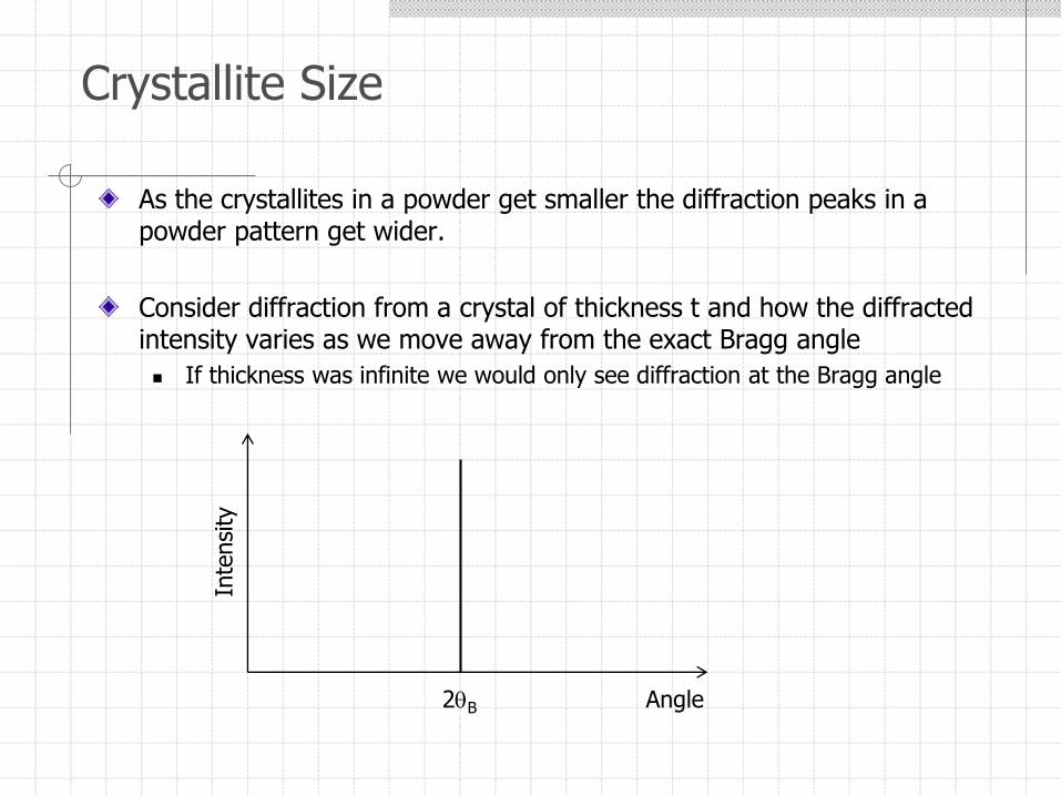
Crystallite Size

As the crystallites in a powder get smaller the diffraction peaks in a powder pattern get wider.

Consider diffraction from a crystal of thickness t and how the diffracted intensity varies as we move away from the exact Bragg angle

If thickness was infinite we would only see diffraction at the Bragg angle

Inte

nsi

ty

Angle2B

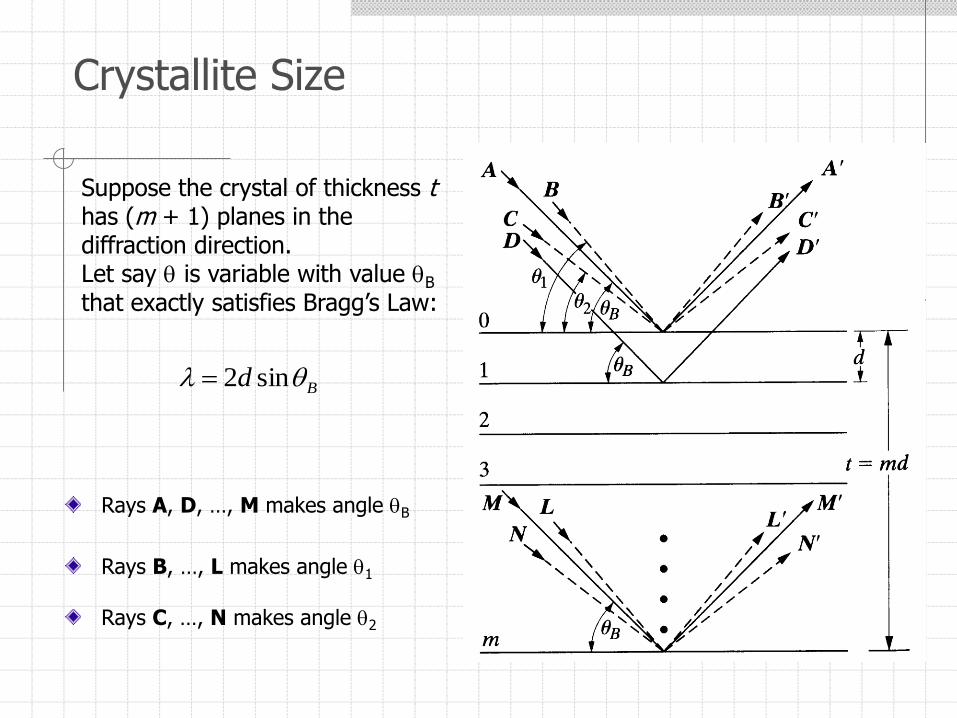
Crystallite Size

Rays A, D, …, M makes angle B

Rays B, …, L makes angle 1

Rays C, …, N makes angle 2

Suppose the crystal of thickness thas (m + 1) planes in the diffraction direction.Let say is variable with value B

that exactly satisfies Bragg’s Law:

Bd sin2

Crystallite Size

For angle B diffracted intensity is maximum

For 1 and 2 – intensity is 0.

For angles 1 > > 2 – intensity is nonzero.

Real case Ideal case

2121 222

1 B

The Scherrer Equation

.1sin2

,1sin2

2

1

mt

mt

.2

sin2

cos2

,sinsin

2121

21

t

tSubtracting:

1 and 2 are close to B, so:

.22

sin

,2

2121

21

B

Thus:

B

B

Bt

t

cos

,cos2

2 21

The Scherrer Equation

More exact treatment (see Warren) gives:

BBt

cos

94.0 Scherrer’s formula

Suppose = 1.54 Å, d = 1.0 Å, and = 49o:

for crystal size of 1 mm, B = 10-5 deg.for crystal size of 500 Å, B = 0.2 deg.

• Peak width B varies inversely with the crystallite size.

• The proportionality constant, K, is usually 0.94 and is valid for spherical crystals with cubic symmetry when B is taken as full width at half maximum (FWHM).

• The proportionality constant, K, is 0.89 for spherical crystals with cubic symmetry when B is taken as integral breadth.

• K sometimes is rounded up to 1.

• K might vary from 0.62 to 2.08.

Instrument broadening has to be subtracted

Peak Width

Full Width at Half Maximum (FWHM):

Width of the peak at half intensity value between background and peak maximum intensity.

Integral Breadth:

Total area under the peak divided by the peak height.

Same as the width of a rectangle which has the same area and the same height as the peak

FWHM

Williamson-Hall Plot

Size broadening (Scherrer equation):

Strain broadening:

Convoluted broadening:

𝐵𝑡 2𝜃 =𝐾𝜆

𝑡 𝑐𝑜𝑠𝜃

𝐵𝜀 2𝜃 = 4𝜀 𝑡𝑎𝑛𝜃

𝐵𝑡𝑜𝑡 2𝜃 = 𝐵𝑡 2𝜃 +𝐵𝜀 2𝜃 =𝐾𝜆

𝑡 𝑐𝑜𝑠𝜃+ 4𝜀 𝑡𝑎𝑛𝜃

𝐵𝑡𝑜𝑡𝑐𝑜𝑠𝜃 =𝐾𝜆

𝑡+ 4𝜀 𝑠𝑖𝑛𝜃

Slope =

4𝑠𝑖𝑛𝜃

𝐾𝜆

𝑡

𝐵𝑡𝑜𝑡𝑐𝑜𝑠𝜃

Instrument broadening has to be subtracted

Corrections for Instrumental Broadening

There is a link between peak width and crystallite size/strain, but other sources of peak broadening have to be considered when analyzing diffraction data

Instrumental broadening:

slit widths

sample size

penetration in the sample

imperfect focusing

unresolved 1 and 2 peaks

or wavelengths widths where 1 and 2 peaks are resolved

To correct for instrumental broadening:

measure the sample

measure under the same conditions the standard with unstrained particles large enough to eliminate particle-size broadening

Corrections for Instrumental Broadening

Lorentzian shape:

Gaussian shape:

Voigt, Pseudo-Voigt: Deconvolute peaks into gaussian and lorentzian fractions and then subtract

instrumental broadening.

𝐵𝑜𝑏𝑠 = 𝐵𝑠𝑖𝑧𝑒+𝐵𝑠𝑡𝑟𝑎𝑖𝑛+𝐵𝑖𝑛𝑠𝑡

𝐵𝑜𝑏𝑠 − 𝐵𝑖𝑛𝑠𝑡 = 𝐵𝑠𝑖𝑧𝑒+𝐵𝑠𝑡𝑟𝑎𝑖𝑛

𝐵𝑜𝑏𝑠2 =𝐵𝑠𝑖𝑧𝑒

2 +𝐵𝑠𝑡𝑟𝑎𝑖𝑛2 +𝐵𝑖𝑛𝑠𝑡

2

𝐵𝑜𝑏𝑠2 − 𝐵𝑖𝑛𝑠𝑡

2 =𝐵𝑠𝑖𝑧𝑒2 +𝐵𝑠𝑡𝑟𝑎𝑖𝑛

2

LorentzianGaussian

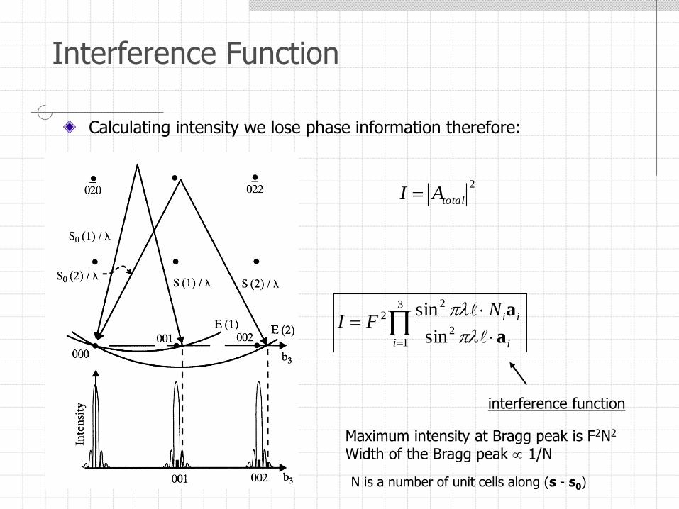
Interference Function

We calculate the diffraction peak at the exact Bragg angle B and at angles that have small deviations from B.

If crystal is infinite then at B intensity = 0.

If crystal is small then at B intensity 0. It varies with angle as a function of the number of unit cells along the diffraction vector (s – s0).

At deviations from B individual unit cells will scatter slightly out of phase.

Vector (s – s0)/ no longer extends to the reciprocal lattice point (RLP).

3210 bbb

sslkh

)(

Interference Function

(1) > B(1) for 001 and (2) > B(2) for 002

If Hhkl = H is reciprocal lattice vector then (s – s0)/ H.

Real space Reciprocal space

Interference Function

We define:

as deviation parameter

HSS 0

Interference Function

In order to calculate the intensity diffracted from the crystal at B, the phase differences from different unit cells must be included.

For three unit vectors a1, a2 and a3:

1

0

332211

1

0

1

0

3

3

2

2

1

1

2exp

N

n

N

n

N

n

total nnni

FA aaass 0

ni – particular unit cellNi – total number of unit cells along ai

332211 bbbHss 0 lkh

From the definition of the reciprocal lattice vector:

Interference Function

1 2 3

1 2 3

332211332211

332211

2exp

2exp

n n n

n n n

total

nnnlkhiF

nnniFA

aaabbb

aaaH

since: ijij ab

321

332211 2exp2exp2expnnn

total anianianiFA

Converting from exp to sines:

332211

3

1

111expsin

sinaaa

a

a

NNNN

FAi i

iitotal

Interference Function

Calculating intensity we lose phase information therefore:

2

totalAI

3

12

22

sin

sin

i i

iiNFI

a

a

interference function

Maximum intensity at Bragg peak is F2N2

Width of the Bragg peak 1/N

N is a number of unit cells along (s - s0)

Interference Function

Crystallite Size

Perfect Crystals

The diffracted intensity calculations make use of ideally imperfect crystals

This is the “kinematical” theory of diffraction

The integrated intensity from a perfect crystal – large and no mosaic blocks – is less than that from an ideally imperfect crystal

Our consideration of Bragg peak width also has some problems. When we have very large perfect crystals the peak width is not zero. The width converges to a finite small value as the size of the crystal increases

We need a better theory!

Dynamical theory is used to treat diffraction in perfect crystals

Perfect Crystals

Dynamical diffraction theory is complicated. It includes the possibility of multiple scattering in a crystal. Diffracted beam is phase shifted by 90° every time it is diffracted within the crystal (this is in addition to the 180°shift on scattering from an individual electron or atom)

Scattering twice off a set of lattice planes K0 to K1 to K2, produces a diffracted beam in the direction of the incident beam but with a 180° phase shift. The resulting destructive interferences reduces the intensity of the beam in the incident direction

This is PRIMARY EXTINCTION

Perfect Crystals

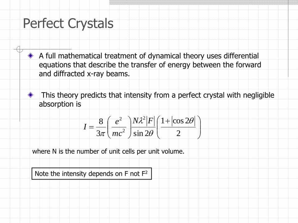
A full mathematical treatment of dynamical theory uses differential equations that describe the transfer of energy between the forward and diffracted x-ray beams.

This theory predicts that intensity from a perfect crystal with negligible absorption is

2

2cos1

2sin3

82

2

2

FN

mc

eI

where N is the number of unit cells per unit volume.

Note the intensity depends on F not F2

Perfect Crystals

The theory also predicts that the peak shape on rocking the crystal in the diffracted beam. The width of this rocking curve is called the Darwin width. Note that at the top of the curve the reflectivity is ~100%.

The width of the curve 2s is given by

2

2cos1

2sin

2

2

2

FN

mc

es

Changes in shape:due to absorption

FWHM, 0, for Darwin curve = 2.12s

For first order reflections:5 arcs < 0 < 20 arcs

Higher order reflections have considerably narrower rocking curves

The Powder Diffraction File

Experience has shown that the ensemble of d-spacings (“d “ s) and intensities (“I “ s) is sufficiently distinctive in order to identify phases

Phase determination can be performed by a comparison of a set of experimental d’’s and I ’s with a database of d -I files

d - spacings are independent of wavelength

Intensities are relative (most intense = 100 or 1000 or 1)

Powder Diffraction File (PDF) Database

1919 -- Hull pointed out that powder diffraction could be used for routine chemical analyses

powder pattern is characteristic of the substance

the patterns of a combination of phases will superimpose

only a small amount is needed

1938 -- Hanawalt, Rinn and Frevel at Dow Chemical compiled diffraction data on about 1000 compounds as 3”x5” file cards and devised a simple means of classifying the data

1942 -- the American Society for Testing Materials (ASTM) published the first edition of diffraction data cards (1300 entries)

Card image for Ce2(SO4)3 from PDF Set 1 as issued in 1941

Source: ICDD

Powder Diffraction File (PDF) Database

1962, the d-I’s, formulas, and PDF numbers were first keyboarded for a computer-readable database.

1969 -- the Joint Committee on Powder Diffraction Standards (JCPDS) was formed as a non-profit corporation to oversee the database

By 1971 the Powder Diffraction File (PDF) contained 21 sets of data with about 21,500 entries

1978 – name change to the International Centre for Diffraction Data (ICDD)

PDF-4 Release 2011

316,291 total datasets

Source: ICDD

Computer Searching of the PDF

Computerization has dramatically improved the efficiency of searching the JCPDS database

Cards are no longer printed – data are on CD-ROM

Numerous third-party vendors have software for searching the PDF database

Computerized “cards” can contain much more crystallographic information

Evolution of the database is continuing…

Experimental Issues and Problems

Searching of the PDF requires high-quality data

accurate line positions are a must!

calibration of camera and diffractometer with known d - spacing standards

careful measurement of line intensities

elimination of artifacts (e.g. preferred orientation)

solid solutions and strains shift peak positions

“garbage in, garbage out” -- poor quality data will usually give a poor match

mixtures of two or more phases

errors in the database

Whole Pattern Fitting

Traditional quantitative phase analysis focuses on the intensities of one or a small number of peaks

Greater accuracy can be obtained by fitting the whole diffraction pattern to what would be expected for a mixture of components

This approach gives an analysis that is an average over all of the peaks, so it is less susceptible to errors that arise from preferred orientation or poor particle statistics

The Rietveld method fits the whole of the diffraction pattern to calculated intensities for the various phases that are present. Gives crystal structure information as well as composition.

XRD on Mars

This image from NASA’s Curiosity rover shows the first sample of powdered rock extracted by the rover’s drill. The image was taken after the sample was transferred from the drill to the rover’s scoop. In planned subsequent steps, the sample will be sieved, and portions of it delivered to the Chemistry and Mineralogy instrument and the Sample Analysis at Mars instrument.

XRD on Mars

Schematic diagram of the CheMin instrument and resulting XRF and XRD data.

Bish et al.

Volume 1 | Part 6 | November 2014 | Pages 514–522 | 10.1107/S2052252514021150

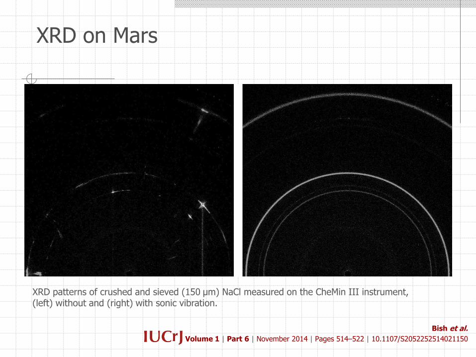
XRD on Mars

XRD patterns of crushed and sieved (150 µm) NaCl measured on the CheMin III instrument, (left) without and (right) with sonic vibration.

Bish et al.

Volume 1 | Part 6 | November 2014 | Pages 514–522 | 10.1107/S2052252514021150

XRD on Mars

A two-dimensional XRD pattern for the Rocknest aeolian bedform (dune).Bish et al.

Volume 1 | Part 6 | November 2014 | Pages 514–522 | 10.1107/S2052252514021150

XRD on Mars

Observed (blue, integrated from the two-dimensional image in Fig.6) and calculated (red) plots from Rietveld refinement using data for Rocknest (∼26.4 h integration, phases listed in Table1).

Bish et al.

Volume 1 | Part 6 | November 2014 | Pages 514–522 | 10.1107/S2052252514021150

Mineral Weight (%)

Plagioclase 30

Forsterite-Fe 16

Augite 11

Pigeonite 10

Magnetite 1.5

Anhydrite 1.1

Quartz 1.0

Sanidine† 1.0

Hematite† 0.8

Ilmenite† 0.9

Amorphous 27

†At or near the detection limit.

First Reported:"LiFePO4: A Novel Cathode Material for Rechargeable Batteries“,A.K. Padhi, K.S. Nanjundaswamy, J.B. Goodenough, Electrochimical Society Meeting Abstracts, 96-1, May, 1996, pp 73.

Excellent candidate for the cathode of rechargeable lithium battery that is inexpensive, nontoxic, and environmentally benign.

Structure of LiFePO4

Padhi, A. K.; Nanjundaswamy, K. S.; Goodenough, J. B. J. Electrochem. Soc. 1997, 144, 1188

Whole Pattern Fitting - Example: LiFePO4

Cathode (LixCoO2: 0 < x < 1)Anode (LixC6: 0 < x < 1)

Commercialized by Sony Corp. in 1991

Limits for the large scale applications:1. Safety2. Cost (Co)

Whole Pattern Fitting - Example: LiFePO4

•When a lithium-based cell is discharging, the lithium is extracted from the anode and inserted into the cathode.•When the cell is charging, the reverse occurs.

Maximum entropy method (MEM)-based whole-pattern fitting of room temperature high-resolution synchrotron X-ray diffraction data for LiFePO4. The incident beam from the bending magnet source was monochromated by a double-crystal Si (111) monochromator, and the diffraction data were collected by a multiple-detector system with flat Ge (111) analysis crystals and scintillation counters. The wavelength was calibrated as 1.206353 Å by powder diffraction data from NIST SRM640c.

Whole Pattern Fitting - Example: LiFePO4

“Experimental visualization of lithium diffusion in LixFePO4”Shin-ichi Nishimura, Genki Kobayashi, Kenji Ohoyama, Ryoji Kanno, Masatomo Yashima & Atsuo YamadaNature Materials 7, 707 (2008) Published online: 10 August 2008

Whole Pattern Fitting - Example: LiFePO4

Whole Pattern Fitting - Example: LiFePO4

Rietveld refinement results for LiFePO4 with neutron diffraction data measured at room temperature in air.

Whole Pattern Fitting - Example: LiFePO4

X-ray diffraction patterns of a mixture of 0.6 LiFePO4 and 0.4 FePO4 recorded at 30 K steps from 298 K to 633 K with magnification of 200 reflections. Bruker AXS D8 ADVANCE powder diffractometer was used with Co-K radiation and linear position-sensitive detector

Vantec-1. Measurement ranges were from 15° to 100°. The measurements were conducted under a high-purity He atmosphere in an Anton Paar HTK 450 temperature-controlled chamber.

Whole Pattern Fitting - Example: LiFePO4

Rietveld refinement results for LiFePO4 with neutron diffraction data measured at room temperature in air.

Rietveld refinement results for Li0.6FePO4 using neutron diffraction data measured at 620 K in Ar.

Whole Pattern Fitting - Example: LiFePO4

Nuclear distribution of lithium calculated by the Maximum Entropy Method (MEM) using neutron powder diffraction data measured for Li0.6FePO4 at 620 K.

(a) Three-dimensional Li nuclear density data shown as blue contours. The brown octahedra represent FeO6 and the purple tetrahedra represent PO4 units.

(b) Two-dimensional contour map sliced on the (001) plane at z = 0.5; lithium delocalizes along the curved one-dimensional chain along the [010] direction, whereas Fe, P and O remain near their original positions.

(c) Two-dimensional contour map sliced on the (010) plane at y = 0; all atoms remain near their original positions.