Different Regions, Differences in Energy Consumption: Do regions
16
Different Regions, Differences in Energy Consumption: Do regions account for the variability in household energy consumption? Hossein Estiri *, Ryan Gabriel, Eric Howard, and Li Wang University of Washington Working Paper no. 134 Center for Statistics and the Social Sciences University of Washington June 14, 2013 * Interdisciplinary PhD program in Urban Design and Planning, College of Built Environments, University of Washington. Email: [email protected]; Web: http://students.washington.edu/hestiri. This working paper was developed in partial fulfillment of the requirement for CS&SS 560 Hierarchical Modeling for the Social Sciences. The authors would like to acknowledge Adrian Dobra for his instructions and supervision throughout this research.
Transcript of Different Regions, Differences in Energy Consumption: Do regions

1
Different Regions, Differences in Energy Consumption: Do regions account for the
variability in household energy consumption?
Hossein Estiri *, Ryan Gabriel, Eric Howard, and Li Wang
University of Washington
Working Paper no. 134
Center for Statistics and the Social Sciences
University of Washington
June 14, 2013
* Interdisciplinary PhD program in Urban Design and Planning, College of Built Environments, University
of Washington. Email: [email protected]; Web: http://students.washington.edu/hestiri. This working paper was
developed in partial fulfillment of the requirement for CS&SS 560 Hierarchical Modeling for the Social
Sciences. The authors would like to acknowledge Adrian Dobra for his instructions and supervision
throughout this research.

2
Abstract
This research aims to discover between-region variability in household energy consumption behaviors, using
multilevel modeling with data from Residential Energy Consumption Survey in 2009. Where past research
focuses on the physical characteristics of housing, our effort in this research centers on between-region
variability and micro-level determinants of residential energy usage. We found significant between-region
variability with household energy usage across the U.S. Results suggest that the association between heating
degree days and energy consumption varies depending on the type of climate that a household lives in.
Further, household energy usage is significantly associated with the race of the householder and income. In
the discussion section, we connect this outcome to racial disparities between whites and non-whites in
location choice, access to housing, and residential stratification. Moreover, the structure of our research
reveals the necessity of multilevel modeling in gaining an accurate picture of residential energy consumption
for more efficient energy conservation policy.
KEY WORDS: Energy Consumption; Residential Sector; Multilevel Modeling; Racial Disparities; Housing
Choice

1
Residential
EnergyConsumption
Household
Building
Home Appliances
Energy Market
Climate
1. Introduction
Global climate change is causing shifts in current climate regions. Energy use in residential
buildings is one of the major sources of carbon dioxide emissions production from cities.
Comprising between 16% and 50% of the total global energy consumption, most of the urban
energy usage comes from building operations (Swan & Ugursal, 2009; Perez-Lombard, Ortiz, &
Pout, 2008). The crucial role of urban areas in shaping global energy demand, as well as the
emergent urban leadership in climate change mitigation and adaptation, has stimulated growing
attention to urban-scale energy consumption information (Parshall, Gurney, Hammer, & Mendoza,
2010).
Nonetheless, compared with other GHG (greenhouse gases) emission production sectors
(e.g. transportation, industry, etc.), the residential sector is largely an indeterminate energy sink (Swan & Ugursal, 2009). Analysis of energy consumption in cities, in general, and in residential
buildings in particular, has seen little policy or financial support. Additionally, suitable data sources
are not easily accessible for research (Ewing & Rong, 2008; Hirst, 1980; Lutzenhiser, 1992). As a
result, research in this area is dispersed across, and separated by, a variety of disciplines, distinct
theoretical orientations, and research methods (Lutzenhiser, 1992; Perez-Lombard, Ortiz, & Pout,
2008).
The residential sector consumes secondary energy in major end-use groups such as space
heating and cooling, domestic hot water, and appliance and lighting. Energy use in these groups is
highly dependent on local climate, the housing unit, home appliances, energy control systems,
energy markets, household characteristics and behaviors (Swan & Ugursal, 2009; Shimoda, Asahi,
Taniguchi, & Mizuno, 2007; Perez-Lombard, Ortiz, & Pout, 2008; Hirst, Goeltz, & Carney, 1982;
Cramer, et al., 1984) (Figure 1).
Figure 1: Determinants of residential energy consumption

2
Determinants of residential energy use can be categorized into contextual and behavioral
domains (Wilson & Dowlatabadi, 2007). Behavioral domains characterize energy consumption
under the rubric of life-styles and consumption behaviors (Lutzenhiser, 1992), most of which
correlate with sociodemographic and economic characteristics of households. On the contextual
domain, along with local climate, energy market, and home appliances, characteristics of the
housing units embrace the main constituents of the contextual domain. There are two groups of
housing unit characteristics that influence energy consumption: construction quality and physical
attributes of a building. In this paper, we focus on the impact of physical attributes of buildings on
energy consumption.
The Effects of Physical Attributes of Buildings on Energy Consumption
An increase in size of residential buildings, which is often associated with an increase home
appliance use, escalates total energy consumption in the residential sector (Shimoda, Asahi,
Taniguchi, & Mizuno, 2007; Ewing & Rong, 2008; Kaza, 2010; Kelly, 2011). Further, residential
energy consumption varies across different housing types (Brounen, Kok, & Quigley, 2012). This
difference is often more pronounced between single-family and multifamily residential buildings
(Kaza, 2010). Ewing and Rong (2008) show that detached single-family units consume more energy
for heating and cooling, in comparison to households living in multifamily housing units.
Households living in detached single-family units consume 54% more energy for heating and 26%
more for cooling in comparison to households living in multifamily units (Ewing & Rong, 2008).
However, the influence of floor area on energy use per unit floor area is negative, suggesting that
energy use increases more slowly than floor area (Hirst, Goeltz, & Carney, 1982).
The Effects of Household Characteristics on Energy Consumption
Energy consumption behaviors of households vary systematically among socioeconomic
groups and across geographic locations (Lutzenhiser, 1992; Brandon & Lewis, 1999). Household
size and composition are important determinants of energy consumption for residential buildings
(O'Neill & Chen, 2002; Kaza, 2010; Brounen, Kok, & Quigley, 2012). Among all socioeconomic
determinants of residential energy use, household size has the largest impact (Kelly, 2011). An
increase in household size is often associated with higher total energy consumption, but a lower per-
capita consumption (O'Neill & Chen, 2002). The impact of household size, is nuanced, and varies
further by household composition (e.g. number of children and adults, sex of household members).
For example, while the presence of children is expected to increase energy use at home (Van Raaij
& Verhallen, 1983), the number of adults has a much larger influence on total energy use than the
number of children (Hirst, Goeltz, & Carney, 1982).
The role of household income on energy consumption indices is consistent in the literature.
Generally, energy consumption indices are positively associated with income (Hirst, Goeltz, &
Carney, 1982; Brandon & Lewis, 1999; Kahn, 2000; Van Raaij & Verhallen, 1983; Santin, 2011;
Brounen, Kok, & Quigley, 2012; O'Neill & Chen, 2002). Yet, there are complexities in the energy
consumption of lower-income groups. While these groups use less energy, they are less able to
reduce their energy use, compared with high-income consumers. That is in part because low-income
households are more likely to reside in older buildings with poor envelope conditions (Santamouris,
Kapsis, Korres, Livada, Pavlou, & Assimakopoulos, 2007).

3
2. Problem statement and conceptual model
Clear understanding of residential energy consumption is the key constituent of effective
energy policy and planning (Hirst, 1980; Brounen, Kok, & Quigley, 2012), which is supposed to be
achieved through research. However, there are at least two issues in the prior research on residential
energy consumption. First, most of the current residential energy debate focuses on aspects of the
physical characteristics of the housing stock and other technical factors, underestimating the role of
residential household behaviors. Second, much of the traditional research on the determinants of
energy use in the residential sector fails to account for complexities and variations in the effect of
housing- and household-related predictors, such as variations across space, and mediations and
interactions between variables.
We posit that energy consumption behaviors might be different across different regions. Our
hypothesis is based on the assumption that macro-level determinants of energy use, such as climate,
energy market, and local and regional regulatory environments can alter residential energy
consumption by changing effects of micro-level variables. This research focuses on household- and
housing-related determinants of residential energy consumption, aiming to evaluate current
household energy consumption patterns to see if there is significant variability between households
in different regions of the U.S.
3. Data and the Substantive Model
We use microdata from the 13th Residential Energy Consumption Survey (RECS), collected
by the U.S. Energy Information Administration in 2009 (U.S. Energy Information Administration,
2013). Since 1978, RECS has collected energy-related data for occupied primary housing units in a
national area-probability sample survey. Using a complex multistage, area-probability design, the
2009 survey collected data from a random sample of 12,083 households in the U.S. To comply with
the structure and purpose of this study, we use listwise deletion and excluded 493 cases from the
original sample size, leading to a sub-sample of 11590 households for this analysis. A set of 12
variables representing total energy use, household and housing units characteristics, local climate,
regional grouping are selected from the initial set of 325 variables collected as part of the RECS
based on our theoretical focus. These variables include: total energy consumption (BTU), housing
type, total square footage, number of rooms, duration of residence, race, income, household size,
housing unit age, heating degree-days, cooling degree-days, and state group.
For the purpose of this study, we consider a two-level data structure. Figure 2 illustrates the
classification diagram of the dataset for our research. 27 state groups define our macro-level
variable, the regions (for the list of state groups see Appendix). Household and housing unit
information institute our micro-level, along with local climate information. Using local climate
variables helps us to control for climate impacts in our model and focus on household-related and
housing-related predictors of energy consumption.
Households
Regions
Figure 2: Classification diagram of this study's two-level nested structure: households in state groups

4
4. Methods
Before developing our multilevel model, descriptive statistics and histograms are generated
for each of the variables. We recode or transform variables when appropriate. First, the response
variable, total energy usage (BTU), is the square root transformed in order to produce a more
normal distribution.
Figure 3: Histograms illustrating the square root transformation of the response variable Total Energy Usage in BTUs
Also, the housing type covariate includes mobile homes into the single family detached
category, as the mobile home category has a relatively low number of responses. The covariate for
housing unit age is recoded to produce a smoother distribution. And the duration of residence is a
binary predictor with one indicating the household has moved in within the past four years. The
household income variable is recoded so that each of the income groupings represents a change of
$10,000. Finally, the total square footage variable is log transformed to produce a more normal
distribution. Descriptions of each of these covariates are presented in Table 1. The correlations
between each pair of variables can be seen in Figure 4. After the data preparation steps are
complete, the model selection process is started.
Table 1: Variable names and descriptions
Variable Name Variable Description
HTYPE1 Represent house type: 1=single-family detached, 2=single-family attached, 3=apartments with 2-4
units, and 4=apartments with more than 5 units.
TOTSQFT2 Log of the housing unit total square footage
TOTROOMS Total number of rooms in the housing unit
DOR1 A binary variable representing short duration of residents (1= moved in less than 4 years)
MAJORITY A binary variable representing whether or not the householder is White only (non-Hispanic)
HHSIZE Number of household members
HHINC2 2009 gross household income-in 10k intervals
H_AGE2 Age of the housing unit in 4-year intervals
HHAGE Age of the householder
HDD30YR Heating degree days, 30-year average 1981-2010, base 65F
CDD30YR Cooling degree days, 30-year average 1981-2010, base 65F
TOTALBTU
Total 2009 energy usage in thousands BTU. (To justify a non-linear functional form and reduce departure from
multivariate normality, we transformed the output variable, total annual energy consumption, in the square root scale)

5
Figure 4: Correlations between each of the variables
The first step in the model selection process is to start with all 11 potential predictor
variables of interest and include them as the fixed-effects elements in our model. Then all possible
nested subsets of this model are calculated. The best fixed-effects model is selected based on the
lowest Bayesian Information Criterion (BIC) score of 126,701. This model includes cooling degree-
days, heating degree-days, housing unit type, household income, household size, total rooms, total
square footages, race, housing unit age, and the age of the householder, and has the following
general form:
𝑇𝑂𝑇𝐴𝐿𝐵𝑇𝑈 = 𝐶𝐷𝐷30𝑌𝑅 + 𝐻𝐷𝐷30𝑌𝑅 + 𝐻𝑇𝑌𝑃𝐸1 + 𝐻𝐻𝐼𝑁𝐶2 + 𝐻𝐻𝑆𝐼𝑍𝐸 + 𝑇𝑂𝑇𝑅𝑂𝑂𝑀𝑆
+ 𝑇𝑂𝑇𝑆𝑄𝐹𝑇2 + 𝑀𝐴𝐽𝑂𝑅𝐼𝑇𝑌 + 𝐻_𝐴𝐺𝐸2 + 𝐻𝐻𝐴𝐺𝐸 + (1|𝑆𝑇𝐴𝑇𝐸𝑆)
Additionally, two potential interaction terms are evaluated by adding them as fixed-effects
into model. These terms comprise the interaction of race and household income and race and
housing type. The model that contains the race and household income interaction term has the
lowest BIC score and shows a significantly better fit using a log likelihood ratio test. The resulting
BIC scores and the p-values from the log likelihood tests are presented in Table 2.
Table 2: BIC score and the results of log likelihood ratio test from adding the interaction terms to the baseline model
Interactions BIC P-Value of log likelihood test against the baseline random-effects model
MAJORITY*HHINC2
and
MAJORITY*HTYPE1
126,694 3.244e-9
MAJORITY*HHINC2 126,673 9.553e-10
MAJORITY*HTYPE1 126,713 1.079e-3
The random-effects model is selected by developing a random intercepts model using the
state groupings. Then a series of models are calculated by allowing the slopes to vary by each one

6
of the micro-level variables individually. By comparing BIC scores the model that allows the slopes
to vary by heating degree-days is shown to be the best fit with a score of 126,439. This model has
the following basic form:
𝑇𝑂𝑇𝐴𝐿𝐵𝑇𝑈 = 𝐶𝐷𝐷30𝑌𝑅 + 𝐻𝐷𝐷30𝑌𝑅 + 𝐻𝑇𝑌𝑃𝐸1 + 𝐻𝐻𝐼𝑁𝐶2 + 𝐻𝐻𝑆𝐼𝑍𝐸 + 𝑇𝑂𝑇𝑅𝑂𝑂𝑀𝑆
+ 𝑇𝑂𝑇𝑆𝑄𝐹𝑇2 + 𝑀𝐴𝐽𝑂𝑅𝐼𝑇𝑌 + 𝐻_𝐴𝐺𝐸2 + 𝐻𝐻𝐴𝐺𝐸 + 𝑀𝐴𝐽𝑂𝑅𝐼𝑇𝑌 ∗ 𝐻𝐻𝐼𝑁𝐶2+ (1 + 𝐻𝐻𝐷30𝑌𝑅 | 𝑆𝑇𝐴𝑇𝐸𝑆)
Each possible combination of the micro-level variables is introduced in conjunction with heating
degree-days in allowing the slopes to vary. Through this process the random slopes model that
includes the race and heating degree-days variables has the overall lowest BIC score of 126,413.
The resulting model has the following form:
𝑇𝑂𝑇𝐴𝐿𝐵𝑇𝑈 = 𝐶𝐷𝐷30𝑌𝑅 + 𝐻𝐷𝐷30𝑌𝑅 + 𝐻𝑇𝑌𝑃𝐸1 + 𝐻𝐻𝐼𝑁𝐶2 + 𝐻𝐻𝑆𝐼𝑍𝐸 + 𝑇𝑂𝑇𝑅𝑂𝑂𝑀𝑆
+ 𝑇𝑂𝑇𝑆𝑄𝐹𝑇2 + 𝑀𝐴𝐽𝑂𝑅𝐼𝑇𝑌 + 𝐻_𝐴𝐺𝐸2 + 𝐻𝐻𝐴𝐺𝐸 + 𝑀𝐴𝐽𝑂𝑅𝐼𝑇𝑌 ∗ 𝐻𝐻𝐼𝑁𝐶2+ (1 + 𝑀𝐴𝐽𝑂𝑅𝐼𝑇𝑌 + 𝐻𝐻𝐷30𝑌𝑅 | 𝑆𝑇𝐴𝑇𝐸𝑆)
We use log likelihood ratio tests to confirm that random-effects varying slopes and
intercepts model have the best fit compared to the fixed-effects and the random-effects varying
intercepts model. The tests between the fixed-effects model and both of the random-effects models
produce a p-value equal to zero. Additionally, the test between the varying intercepts model and the
varying slopes and intercepts also produce a value of zero. These test results indicate that the
varying slopes and intercepts model is the best fit with the available data.
5. Results
The final chosen model has fixed additive effects, fixed effect interaction, random effect
intercepts, and random effect slopes. The dependent variables associated with each are shown in
Table 3 All the variables shown are either significant or included because an interaction term is
significant.
Table 3: Components of the chosen model.
Chosen model
Fixed effects cooling degree days, heating degree days, number of rooms, total sq. ft. size, housing age,
housing type, household income, household size, household age, majority status
Interaction majority status × household income
Random effect grouping states groups
Random effect slopes majority status, heating degree days
Fixed effects
The fixed effect coefficients are shown in Table 4. The actual magnitudes of these
coefficients are not comparable. First, they are the results of a model selection process; the
coefficients do not account for the uncertainty in the model. If the interest is in predicting the
energy consumption of households, Bayesian Model Averaging (BMA) can be used to weigh and
combine the contribution from multiple models. Secondly, the variables have not been standardized.
The ranges of the predictors have a large effect on the size of the coefficients. For example, the

7
binary variable (Majority) has a range of (0, 1), which gives a –18 contribution to the response,
while the variable (HDD30YR) has a range of (0, 13346), which translates to a 159 contribution to
the response over that range.
Table 4: Fixed effects coefficients
Coefficient Estimate Standard Error
Intercept -130.3000 16.6100
Cooling Degree Days 0.0166 0.0017
Heating Degree Days 0.0119 0.0022
Housing Type (Single Family Attached) -13.6000 2.1110
Housing Type (Apartment, 2-4 Units) -11.1300 2.2490
Housing Type (Apartment, 5+ Units) -32.2100 1.9130
Household Income 0.8399 0.2907
Household Size 7.9530 0.4071
Total Rooms 7.0160 0.4038
Total Square Feet 84.0700 3.3370
Majority -18.0700 3.1190
House Age 1.8540 0.1178
Household Age 0.2501 0.0354
Household Income * Majority 1.8960 0.3317
The signs of the coefficients are important for interpretation, to see if they match up with our
scientific intuition about energy consumption. The variables can be grouped into three categories –
residence, household, and climate characteristics. Residence characteristics, which include the total
number of rooms and size of the residence, have positive coefficients. This makes sense intuitively
as larger residences are associated with more energy consumption. Apartments and attached
housing are associated with lower energy usage than single-family detached homes. The age of the
house has a positive association with energy consumption. This association may result from older
homes having poorer insulation and less overall energy efficiency.
Household characteristics contain household size, householder age, household income, and
majority. Household size and householder age are both positively associated with energy
consumption. This indicates that large families use more energy, and that older families may be less
mindful of energy use. Household income also has a positive relationship indicating that richer
families may be consuming more energy. Majority has a negative coefficient; we will consider the
effect of racial characteristic in greater detail below.
Climate characteristics incorporate heating and cooling degree days. Heating degree days is
positively associated with energy consumption, showing the significant impact of electrical heating.
Although cooling degree days is negatively associated with the response variable, its coefficient is
positive after controlling for other variables – mainly the effect of heating degree days. So, for areas
with equally cold winters, the ones with hotter summers may consume more energy. This effect
shows the potential impact of air conditioning.
As seen in the correlation plot (Figure 4), Majority is positively associated with energy
consumption. However, after adjusting for other variables in the model, particularly for heating
8
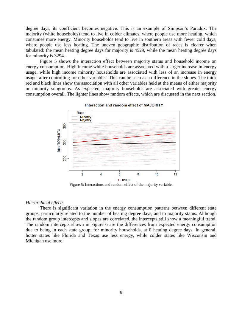
degree days, its coefficient becomes negative. This is an example of Simpson’s Paradox. The
majority (white households) tend to live in colder climates, where people use more heating, which
consumes more energy. Minority households tend to live in southern areas with fewer cold days,
where people use less heating. The uneven geographic distribution of races is clearer when
tabulated: the mean heating degree days for majority is 4529, while the mean heating degree days
for minority is 3294.
Figure 5 shows the interaction effect between majority status and household income on
energy consumption. High income white households are associated with a larger increase in energy
usage, while high income minority households are associated with less of an increase in energy
usage, after controlling for other variables. This can be seen as a difference in the slopes. The thick
red and black lines show the association with all other variables held at the means of either majority
or minority subgroups. As expected, majority households are associated with greater energy
consumption overall. The lighter lines show random effects, which are discussed in the next section.
Figure 5: Interactions and random effect of the majority variable.
Hierarchical effects
There is significant variation in the energy consumption patterns between different state
groups, particularly related to the number of heating degree days, and to majority status. Although
the random group intercepts and slopes are correlated, the intercepts still show a meaningful trend.
The random intercepts shown in Figure 6 are the differences from expected energy consumption
due to being in each state group, for minority households, at 0 heating degree days. In general,
hotter states like Florida and Texas use less energy, while colder states like Wisconsin and
Michigan use more.

9
Figure 6: State effects on estimated energy consumption
The association between heating degree days (HDD) and energy consumption for state
group j is given by the formula:
𝛽HDD + 𝑢HDD,𝑗
The three figures below show random slopes for heating degree days in three different states. The
dashed black line shows the average association between HDD and energy consumption, 𝛽𝐻𝐷𝐷 .
Florida has lower energy consumption than average, but it rises more quickly when the weather gets
cold. Wisconsin has higher energy consumption than average, but it does not change significantly
with cold weather. The effect here may be due to regional differences in housing that’s not in our
model, such as the amount of insulation; or it may be due to regional household behavior
differences.
Figure 7: Random slope for FL
Figure 8: Random slope for WI

10
The slope for the state group Alaska, Hawaii, Oregon, and Washington show that when there
is heterogeneity in climate pattern in a state group, it can overwhelm the random effect we are
trying to capture. For this group, the slope is determined by the differences between Hawaii (low
energy usage, warm climate) and Alaska (high energy usage, cold climate).
The difference between majority and minority for state group j, controlling for other
variables, is given by
𝛽majority + 𝛽interaction × 𝐻𝐻𝐼𝑁𝐶2 + 𝑢majority,𝑗
Figure 5 in the previous section showed the random effects of majority status along with its
interaction with household income, for each of the states. The random effect lines are plotted while
holding all the other variables constant at the means for that state. Below, two of the states are
selected, and their state effects are plotted in thick dashed lines. In Michigan, an average white
household uses less energy than an average minority family, though the difference decreases for
higher income. In Texas, minority households use less energy, and the difference increases for
higher income.
Figure 9: Random slope for AK, HI, OR, & WA
Figure 10: Random slope for Michigan Figure 11: Random slope for Texas

11
6. Summary and Conclusions
With this research we have endeavored to discover if there is between-region variability in
household energy consumption behaviors. We find significant between-region variability with
household energy usage across the U.S. Our results suggest that heating degree days vary depending
on the type of climate that a household is in. For instance, households in areas of the country that
experience colder weather tend use more energy than those households that reside in warmer
climates. A salient theoretical finding from our investigation is that household energy usage is
significantly associated with the race of the householder and income. This is not surprising. Past
research finds that racial disparities between whites and non-whites exist in almost every social
circumstance. Non-whites generally have lower incomes, higher negative health outcomes, and
detrimental neighborhood conditions, along with other socially deleterious circumstances. Thus, this
finding is telling in that it mirrors minority groups’ experiences, especially blacks, with residential
stratification. Research evinces that as blacks increase in education and income that they are unable
to gain access to white neighborhoods. Some argue that this is due to preferences – that races tend
to prefer in-group solidarity – but others point to discrimination as the main driver of this
phenomenon. What might be occurring in our research is that we are capturing an outcome of
residential housing stratification. Since a large proportion of blacks are living in urban cores they
are on average using less household energy as compared to suburban whites.
We readily acknowledge the limitations of this study. First, mindfulness is necessary when
making causal statements from a model. A regression study does not give any evidence of the
direction or structure of causality between variables. The interpretations above are speculations
based on prior knowledge. Structural equations modeling (SEM) analysis may provide stronger
evidence of causation. Also, our study has limits because we focus on white versus non-white
differences in energy usage based on income. Disaggregating non-whites into other racial categories
will provide a clearer picture of the differences in energy consumption behavior based on race.
Furthermore, prospective studies should break up regions into specific states. Our study has 27 state
groups, which are roughly culled together based on geographic closeness, but there are exceptions.
For example, we have a grouping that includes Alaska, Hawaii, Oregon and Washington. Where
Oregon and Washington are similar in climate, Alaska and Hawaii could not be any different.
Consequently, having all 50 states will eliminate that source of bias.
Our research, being explorative, is effective at defining key variables that are essential in the
investigation of energy consumption within households. Where past research focuses on the
physical characteristics of housing, our efforts center on between-region variability and micro-level
determinants of residential energy usage. We explore the role of household energy behaviors, which
the understanding of is essential to future energy policies. Moreover, the structure of our research
reveals the necessity of multilevel modeling in gaining an accurate picture of residential energy
consumption.
REFERENCES
Beguin, H. (1982). The Effect of Urban Spatial Structure on Residential-Mobility. Annals of Regional
Science , 16-35.
Boehm, T. P. (1982). A Hierarchical Model of Housing Choice. Urban Studies , 17-31.

12
Brandon, G., & Lewis, A. (1999). Reducing Household Energy Consumption: A qualitative and quantitative
field study. Journal of Environmental Psychology , 75-85.
Brounen, D., Kok, N., & Quigley, J. M. (2012). Residentialenergy use and conservation: Economics and
demographics. European Economic Review , 931–945.
Chan, S. (2001). Spatial Lock-in: Do Falling House Prices Constrain Residential Mobility? Journal of Urban
Economics , 567-586.
Chevan, A. (1971). Family Growth, Household Density, and Moving. Demography , 451-458.
Clark, W. A., & Dieleman, F. M. (1996). Households and Housing: Choice and Outcomes in the Housing
Market. New Brunswick, New Jersey: Center for Urban Policy Research, Rutgers.
Clark, W. A., Deurloo, M. C., & Dieleman, F. M. (1984). Housing Consumption and Residential Mobility.
Annals of the Association of American Geographers , 29-43.
Cramer, J. C., Hackett, B., Craig, P. P., Vine, E., Levine, M., Dietz, T. M., et al. (1984). Structural-
Behavioral Determinants of Residential Energy Use: summer electricity use in Davis. Energy , 207-216.
Ewing, R., & Rong, F. (2008). The impact of urban form on US residential energy use. Housing Policy
Debate , 1-30.
Hirst, E. (1980). Review of Data Related to Energy Use in Residential and Commercial Buildings.
Management Science , 857-870.
Hirst, E., Goeltz, R., & Carney, J. (1982). Residential energy use: analysis of disaggregate data . Energy
Economics , 74-82.
Kahn, M. E. (2000). The environmental impact of suburbanization. Journal of Policy Analysis and
Management , 19 (4), 569–586.
Kaza, N. (2010). Understanding the spectrum of residential energy consumption: A quantile regression
approach. Energy Policy , 6574–6585.
Kelly, S. (2011). Do homes that are more energy efficient consume less energy?: A structural equation model
of the English residential sector. Energy , 5610–5620.
Lutzenhiser, L. (1992). A Cultural Model of Household Energy Consumption. Energy , 47-60.
Norman, J., MacLean, H. L., & Kennedy, C. A. (2006). Comparing High and Low Residential Density: Life-
Cycle analysis of energy use and greenhouse gas emissions. Journal of Urban Planning and Development .
O'Neill, B. C., & Chen, B. S. (2002). Demographic Determinants of Household Energy Use in the United
States. Population and Development Review , 53-88.
Parshall, L., Gurney, K., Hammer, S. A., & Mendoza, D. (2010). Modeling energy consumption and CO2
emission at the urban scale: methodological challenges and insights from the United States. Energy Policy ,
4765-4782.
Perez-Lombard, L., Ortiz, J., & Pout, C. (2008). A review on buildings energy consumption information .
Energy and Buildings , 394-398.
Santamouris, M., Kapsis, K., Korres, D., Livada, I., Pavlou, C., & Assimakopoulos, M. (2007). On the
relation between the energy and social characteristics of the residential sector. Energy and Buildings , 39 (8),
893–905.

13
Santin, O. G. (2011). Behavioural Patterns and User Profiles related to energy consumption for heating.
Energy and Buildings , 43 (10), 2662–2672.
Shimoda, Y., Asahi, T., Taniguchi, A., & Mizuno, M. (2007). Evaluation of city-scale impact of residential
energy conservation measures using the detailed end-use simulation model. Energy , 1617-1633.
Swan, L. G., & Ugursal, V. I. (2009). Modeling of end-use energy consumption in the residential sector: A
review of modeling techniques. Renewable and SUstainable Energy Reviews , 1819-1835.
U.S. Energy Information Administration. (2012). 2009 RECS Survey Data. Retrieved from CONSUMPTION
& EFFICIENCY- RESIDENTIAL ENERGY CONSUMPTION SURVEY (RECS):
http://www.eia.gov/consumption/residential/data/2009/#microdata
U.S. Energy Information Administration. (2013). 2009 RECS Survey Data. Retrieved from CONSUMPTION
& EFFICIENCY- RESIDENTIAL ENERGY CONSUMPTION SURVEY (RECS):
http://www.eia.gov/consumption/residential/data/2009/#microdata
U.S. Energy Information Administration. (2010). Annual Energy Review 2010. Retrieved from U.S. Energy
Information Administration: http://205.254.135.24/totalenergy/data/annual/pdf/aer.pdf
Van Raaij, W. F., & Verhallen, T. M. (1983). A behavioral Model of Residential Energy Use. Journal of
Economic Psychology , 39-63.
Wilson, C., & Dowlatabadi, H. (2007). Model of Decision Making and Residential Energy Use. Annual
Review of Environment and Resources , 169-203.

14
APPENDIX
Table A1: 27 State Groupings
1
2
3
4
5
6
7
8
9
10
11
12
13
14
15
16
17
18
19
20
21
22
23
24
25
26
27
Connecticut, Maine, New Hampshire, Rhode Island, Vermont
Massachusetts
New York
New Jersey
Pennsylvania
Illinois
Indiana, Ohio
Michigan
Wisconsin
Iowa, Minnesota, North Dakota, South Dakota
Kansas, Nebraska
Missouri
Virginia
Delaware, District of Columbia, Maryland, West Virginia
Georgia
North Carolina, South Carolina
Florida
Alabama, Kentucky, Mississippi
Tennessee
Arkansas, Louisiana, Oklahoma
Texas
Colorado
Idaho, Montana, Utah, Wyoming
Arizona
Nevada, New Mexico
California
Alaska, Hawaii, Oregon, Washington