Diapositive 1 - astro.ulg.ac.bedupret/cours-structurevol1-ang2017.pdf · 1 . Ψ. 2 . Ψ. 3 . Else...
187
Stellar Structure SPAT0044 Marc-Antoine Dupret Associate Professor email: [email protected] tel: 04 3669732 Bât. B5c, 1 er étage Slides: https://www.astro.ulg.ac.be/~dupret/
Transcript of Diapositive 1 - astro.ulg.ac.bedupret/cours-structurevol1-ang2017.pdf · 1 . Ψ. 2 . Ψ. 3 . Else...

Stellar Structure SPAT0044
Marc-Antoine Dupret Associate Professor email: [email protected] tel: 04 3669732 Bât. B5c, 1er étage Slides: https://www.astro.ulg.ac.be/~dupret/

Goals of the course • Physical processes inside the stars
stars = laboratories of fundamental physics - Quantum physics (radiation - matter) and nuclear physics - Thermodynamics and quantum statistical physics
- Hydrodynamics
• Presentation of simple approximations enabling a
mathematical analysis of the stellar properties
• Link theory - observations
The Hertzsprung-Russell diagram
Lum
inos
ity
Color – spectral type Effective temperature ~ surface temperature
Stars of different masses,
different ages
Different positions in the HR diagram
L = Luminosity = Power radiated
by the star
Ejnar Hertzsprung Henry Norris Russell (1910)
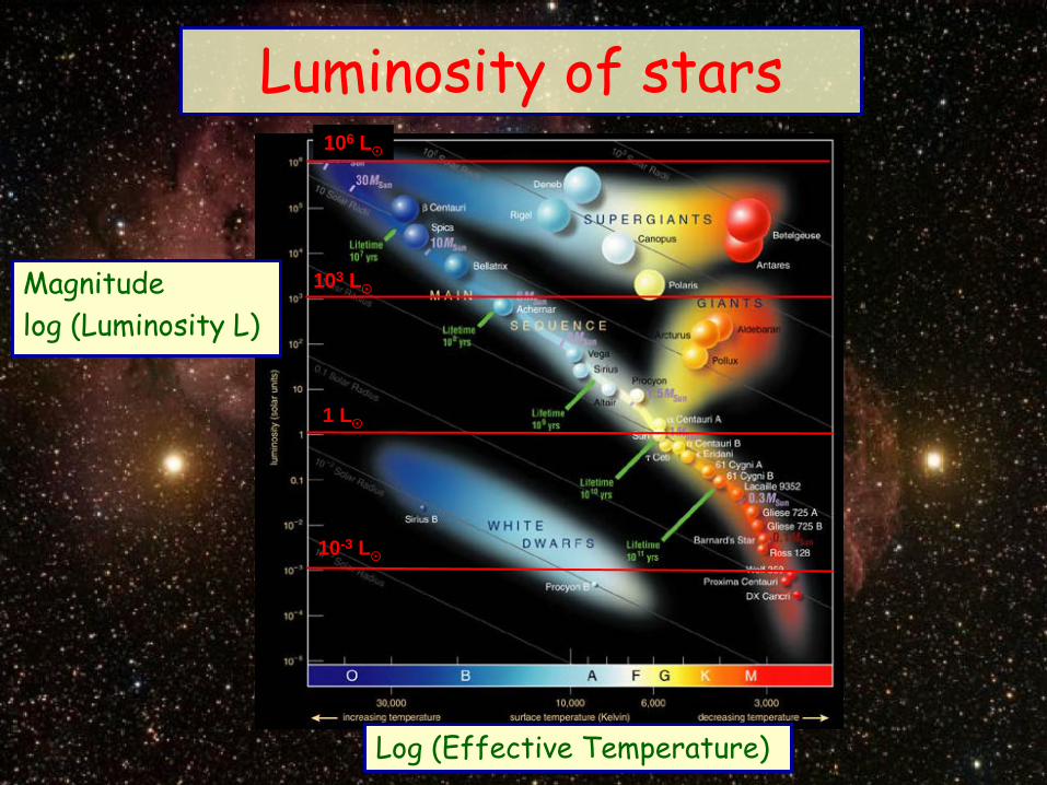
Magnitude log (Luminosity L)
106 L¯
1 L¯
Luminosity of stars
103 L¯
10-3 L¯
Log (Effective Temperature)
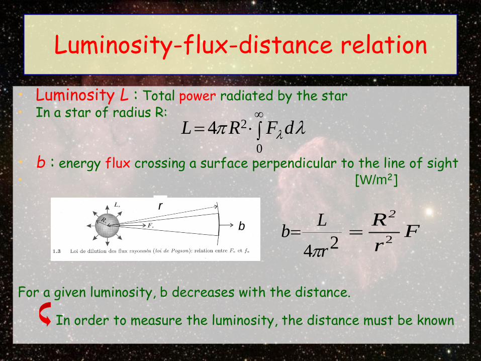
Luminosity-flux-distance relation
• Luminosity L : Total power radiated by the star • In a star of radius R:
• b : energy flux crossing a surface perpendicular to the line of sight • [W/m2]
For a given luminosity, b decreases with the distance.
In order to measure the luminosity, the distance must be known
2
04L R F dλπ λ
∞= ⋅ ∫
24 r
Lbπ
=b
r
FrR2
2 =

Hertzsprung-Russell diagram
Stars whose distance was measured by the Hipparcos satellite
(parallax method)
d?
α α’
b MB – MV
MV
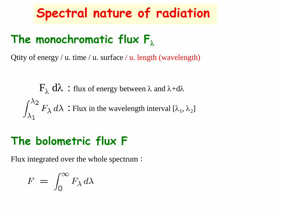
The monochromatic flux Fλ
Qtity of energy / u. time / u. surface / u. length (wavelength)
Fλ dλ : flux of energy between λ and λ+dλ
: Flux in the wavelength interval [λ1, λ2]
The bolometric flux F
Flux integrated over the whole spectrum :
Spectral nature of radiation
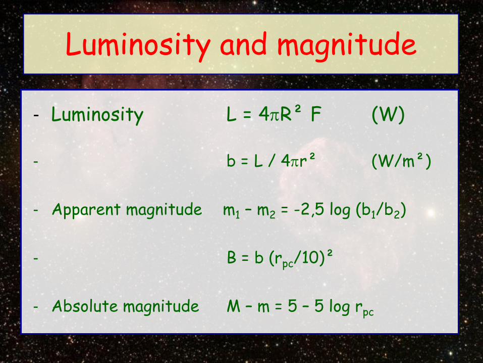
Luminosity and magnitude
- Luminosity L = 4πR² F (W)
- b = L / 4πr² (W/m²)
- Apparent magnitude m1 – m2 = -2,5 log (b1/b2)
- B = b (rpc/10)²
- Absolute magnitude M – m = 5 – 5 log rpc

The black body spectrum
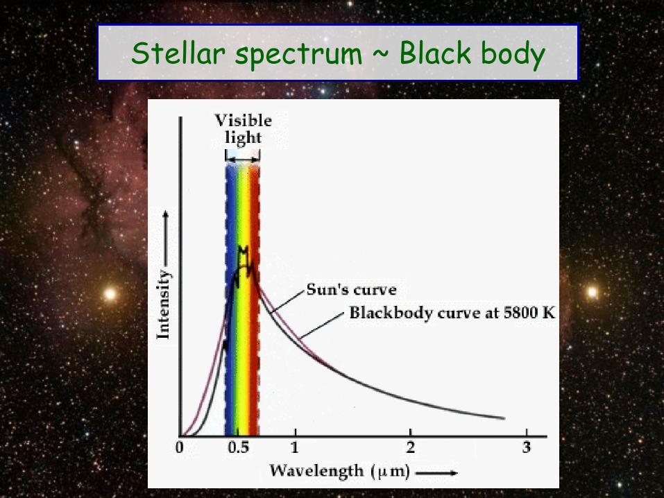
Stellar spectrum ~ Black body

o Planck function
o Stefan-Boltzmann law
o Wien law
max0,29( )( )
cmT K
λ =
Black body laws
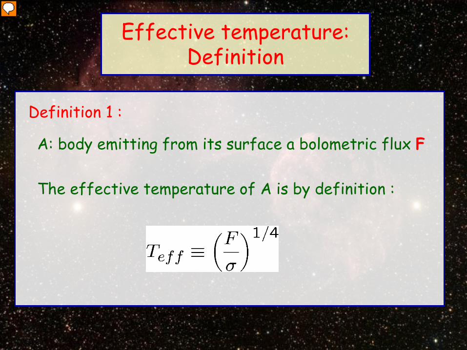
Definition 1 :
A: body emitting from its surface a bolometric flux F
The effective temperature of A is by definition :
Effective temperature: Definition
Presenter
Presentation Notes
ˈtɛmprɪtʃə

The effective temperature of an emitting body is the temperature of a hypothetical black body emitting the same bolometric flux.
For a spherical symetric body of radius R and luminosity L, we have by definition :
L = 4πR²σTeff4
Definition 2 :
Any body : F = σ Teff4
Black body : F = σ T4
Effective temperature: Definition
Presenter
Presentation Notes
haɪpəˈθɛtɪkəl language abuse

Magnitude log (Luminosity L)
30000 K
Effective temperatures of stars
10000 K
Log (Effective Temperature) 3000 K

Size of stars
•Size of stars : 4 ²4 effT
RLF σ
π==
- Main Sequence stars have a restricted range of radii
- Supergiants are thousands times larger than the Sun
- Giants are ten-hundred times larger than the Sun
- White dwarfs are one hundred times smaller than the Sun
Cst T log 4 Rlog 2 Llog eff ++=

Magnitude log (Luminosity L)
Stellar sizes
Log (Effective Temperature)

Hertzsprung-Russell diagram
The main sequence
Stellar source of energy: Thermonuclear reactions
Longest Phase : Fusion of hydrogen into helium
Our Sun is a main sequence star
Most stars are in this phase
M ~ 100 M¯
They occupy a specific region of the HR diagram: The main sequence
M ~ 0.1 M¯

Red giants
Phase of core helium fusion into carbon and oxygen,
and/or shell hydrogen fusion
The core of a red giant is very dense,
its envelope is huge (van encompass the earth orbit)
M ~ 100 M¯
M ~ 0.1 M¯
Hertzsprung-Russell diagram

White dwarfs
Slow cooling …
End of the life of our Sun: Small and dense (R ~ 0.01 R¯ , ρ ~ 1 ton / cm3)
M ~ 100 M¯
M ~ 0.1 M¯
Hertzsprung-Russell diagram
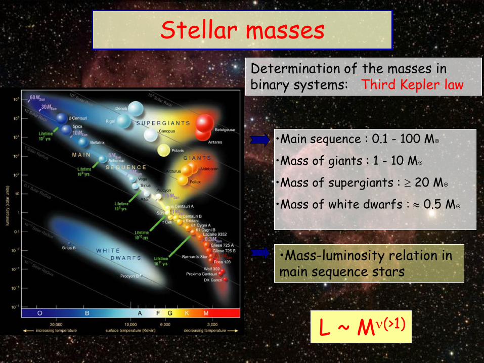
Stellar masses Determination of the masses in binary systems: Third Kepler law
•Main sequence : 0.1 - 100 M
•Mass of giants : 1 - 10 M
•Mass of supergiants : ≥ 20 M
•Mass of white dwarfs : ≈ 0.5 M
•Mass-luminosity relation in main sequence stars
L ~ Mν(>1)

3000 K < Teff < 100000 K
0.08 M < M < 100 M
…0… < L < 106 L
…0… < R < 1000 R
Pop I – Pop II ⇒ X, Y, Z
Characteristics of stars

Our Sun
L = 4π R2σTeff4
Radius = 0.697 £ 106 km
Can be measured, knowing: - Its distance d - Its angular diameter θ
Luminosity = 3.826 £ 1026 W Can be measured, knowing :
- Its distance d - The flux f received on earth
R = d tg θ/2
L = 4π d2 f
Effective temperature = 5777 K ~ Surface temperature
Obtained from its definition :
Mass = 1.989 £ 1030 kg From the third Kepler law:
GM = 4π2 a3/P2

24 rdrdm ρπ=
drr dVdm 2 4 = = πρρ
Internal characteristics of stars
Spherical Symetry Only one space dimension: r
Masse
m
dm
Mass of each spherical shell of thickness dr
~ 1.4£103 kg/m3
Sun :

A gas sphere in hydrostatic equilibrium
The resultant force on each material volume
= 0

Sphere of gas in hydrostatic equilibrium
2 g r
GmdrdP
−=−= ρρ0 =∑F
dr
Equilibrium of the forces :
dmr
GmdrgrPM
rm
R
r
4
)()(
4∫∫ ==
πρ
Resultant force on an infinitesimal volume (1 m2 section) :
Pressure : -P(r+dr) + P(r) (surface force) Weight : -ρ g dr (volume force)
Integrated form :
-P(r+dr)
P(r)
g dm
( P(R) = 0 )

Sun, simplified model of constant density :
~ 5£1014 Pa
21 on accelerati Radial
rmG
drdP - −=
ρ
Dynamical time ~ free fall time
(pressure suppressed) GM
3
dynR t =22
dyntR
RGM
=
Sun : tdyn = 26 min << stellar evolution time
Out of equilibrium state:
Order of magnitude:
During the main part of the stellar life, hydrostatic equilibrium Exception : Explosion of a supernova (dynamical instability)
0 == ∑Fdm
γ

r£ (rP/ρ) = -(1/ρ2) rρ£r P = (1/2) r(Ω2) £ r(s2)
Rotational of the equilibrium equation s es = (1/2) r(s2)
For a rigid or cylindrical rotation (Ω(s)): rρ£rP = 0
Isobars = Iso-density = Isotherms : P(Ψ), ρ(Ψ), T(Ψ), …
Ψ = Total Potential =
Ψ1
Ψ2
Ψ3
Else (more complex differential rotation of real cases):
Isobars ≠ Iso-density ≠ Isotherms
Baroclinity
Fast rotation and hydrostatic equilibrium
s = r sinθ es = rs
Critical speed : if Veq = Ω R > Vcrit ¼ (GM/R)1/2 ,
Centrifugal force > gravity ) the envelope is expelled
Stars can rotate fast ) centrifugal force:
rP/ρ = -rφ + Ω2 s es
) Deformation of the star
Ω2 s es
Presenter
Presentation Notes
Break-up, disintegration

Stars can rotate fast ) centrifugal force:
Fast rotation and hydrostatic equilibrium
rP/ρ = -rφ + Ω2 r sinθ es
) Deformation of the star
) All quantities (T, P, ρ, F, …) depend on 2 space dimensions (r, θ) ) much harder to solve
Critical speed : if Veq = Ω R > Vcrit ¼ (GM/R)1/2 ,
Centrifugal force > gravity ) the envelope is expelled
Some stars (Be stars, …) are not far away from that !
Influence of rotation
Affects the stellar structure and evolution : - 2D structure - Transport processes
Affects spectroscopic and photometric observables (Teff , …),
Because at the photosphere: F(θ), ge(θ)
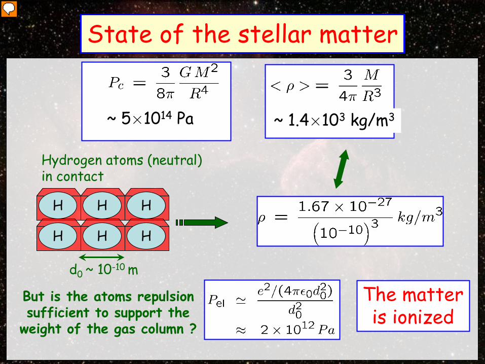
State of the stellar matter
~ 5£1014 Pa
H H
H
H
H H
d0 ~ 10-10 m
Hydrogen atoms (neutral) in contact
~ 1.4£103 kg/m3
But is the atoms repulsion sufficient to support the
weight of the gas column ?
The matter is ionized
Presenter
Presentation Notes
ad absurdum argument
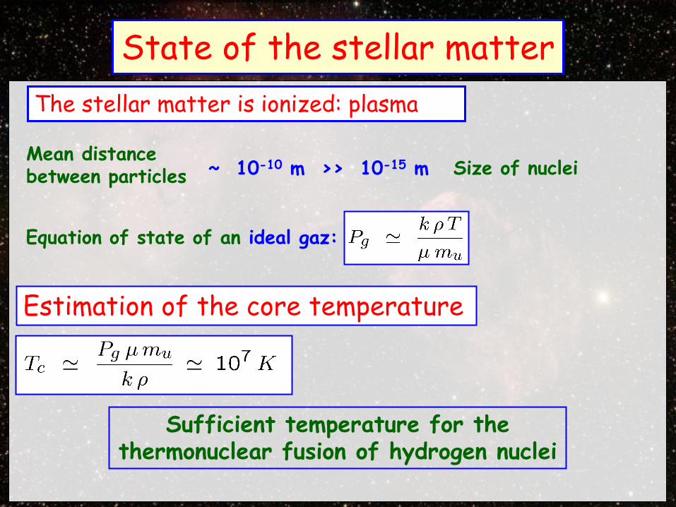
Mean distance between particles
The stellar matter is ionized: plasma
Size of nuclei ~ 10-10 m >> 10-15 m
Equation of state of an ideal gaz:
Estimation of the core temperature
Sufficient temperature for the thermonuclear fusion of hydrogen nuclei
State of the stellar matter
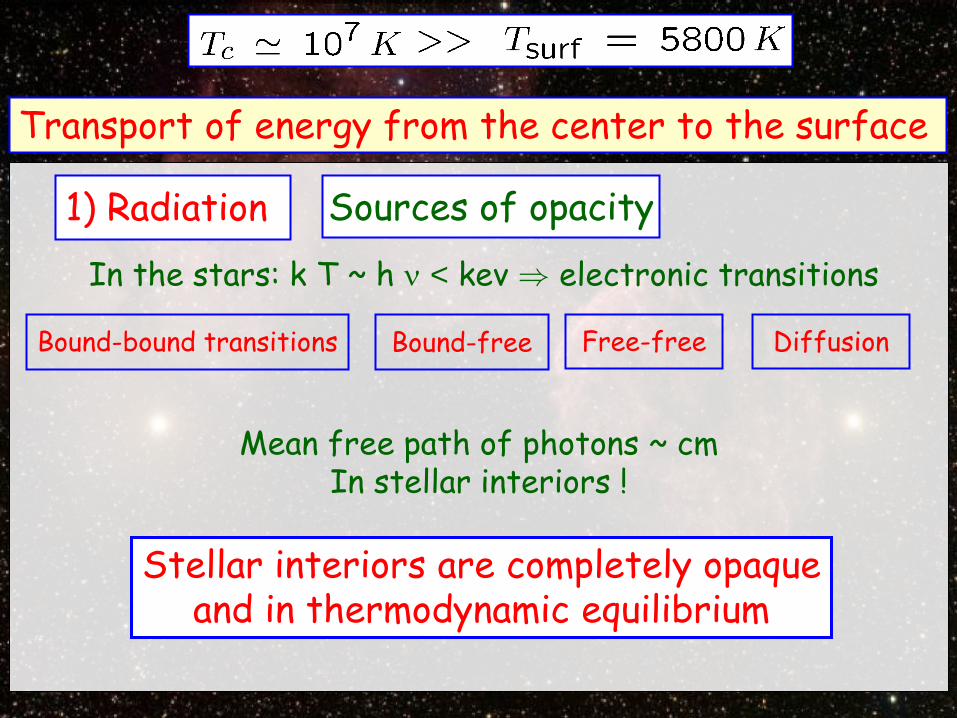
1) Radiation
Transport of energy from the center to the surface
Sources of opacity
Bound-bound transitions
In the stars: k T ~ h ν < kev ) electronic transitions
Bound-free Free-free Diffusion
Mean free path of photons ~ cm In stellar interiors !
Stellar interiors are completely opaque and in thermodynamic equilibrium

Transport of energy (from the center to the surface)
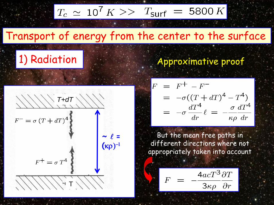
1) Radiation
In stellar interiors:
Mean free path of photons :
= (κρ)-1 ¼ 2cm <<
dr / dlnT, dr/dln P, …
Opaque interior
Matter-radiation thermodynamic equilibrium
Stefan law :
Planck law :
1) Radiation
dTTdTTL
3
4
4 )
σ
σ
=
+( =4T σ
T+dT
T
~ = (κρ)−1
Approximative proof
But the mean free paths in different directions where not
appropriately taken into account
Transport of energy from the center to the surface

1) Radiation Rigorous proof Solution of the radiative
transfer equation:
Radiative transfer equation
θ
* 2 π µ and integration
2/3
Rosseland mean
0

1) Radiation
κ % ) |dT/dr| %
dTTdTTL
3
4
4 )
σ
σ
=
+( =4T σ
T+dT
T
Gradient of T L
Tcenter >> Tsurface
Whatever the source of energy
For a fixed L
Example: partial ionization zones
Transport of energy (from the center to the surface)

2) Convection
m m
If (∆ρ)e < (∆ρ)m
Archimedes force upwards
Convectively unstable medium
Transport of energy (from the center to the surface)

2) Convection
ρe < ρm Convectively unstable medium
if and only if :
Temperature criterion ? Pressure equilibrium:
P=RρT/µ Ideal gas
Te /µe > Tm / µm m m
Transport of energy (from the center to the surface)
Pe = Pm
Pe = R ρe Te / µe = Pm = R ρm Tm / µm
ρe < ρm
Te > Tm If µe = µm

2) Convection
|dlnT/dr|e < |dlnT/dr|m (∆T/T)e > (∆T/T)m
∆ P < 0
(dlnT/dlnP)e < (dlnT/dlnP)m
Transport of energy !
m m
∆ T < 0
Transport of energy (from the center to the surface)
Convectively unstable medium if and only if : Te > Tm

2) Convection
m m
(dlnT/dlnP)e < (dlnT/dlnP)m
Efficient convection Negligible radiative loss
(dlnT/dlnP)e = ∂ lnT/∂ lnP|s ´ rad
(dlnT/dlnP)m ´ r > rad
Transport of energy (from the center to the surface)
Convectively unstable medium if and only if :
Convectively unstable medium if and only if :
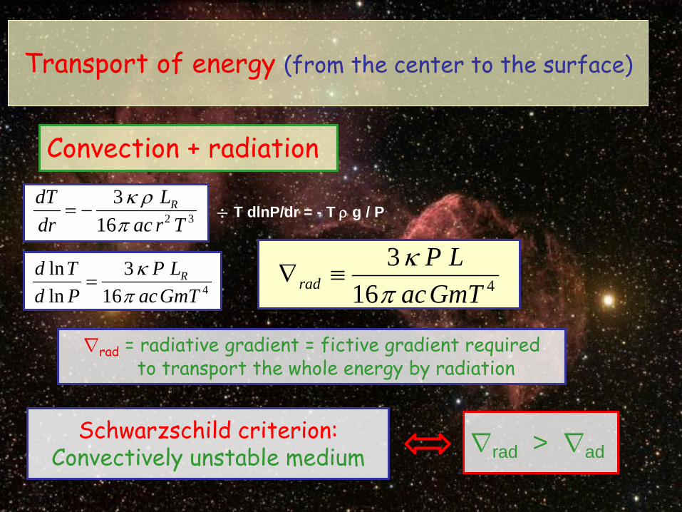
Convection + radiation
rrad = radiative gradient = fictive gradient required to transport the whole energy by radiation
32163
TracL
drdT R
πρκ
−= ¥ T dlnP/dr = - T ρ g / P
4163
lnln
GmTacLP
PdTd R
πκ
= 4163
GmTacLP
rad πκ
≡∇
rrad > rad
Transport of energy (from the center to the surface)
Schwarzschild criterion: Convectively unstable medium

rrad > rad Schwarzschild criterion:
Convectively unstable medium
4163
GmTacLP
rad πκ
≡∇Convection typically appears when :
L/m Very high
Nuclear reactions only near the center
Convective core
κ (opacity) very high
Partial ionization zones near the surface
Convective envelope
Transport of energy (from the center to the surface)
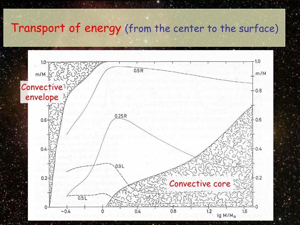
Convective core
Convective envelope
Transport of energy (from the center to the surface)

A small (r - rad) is sufficient
In the deep layers where convective transport
is very efficient r ' rad ' 2/5
Fully ionized gas
Very high heat capacity
Fc = ρ cp Vc,r ∆T (Enthalpy flux) ¼ ρ cpT (P/ρ)1/2α2(r - rad)3/2
Mixing-length theory (very approximative !)
Transport of energy (from the center to the surface)
How efficient is this energy transport ?
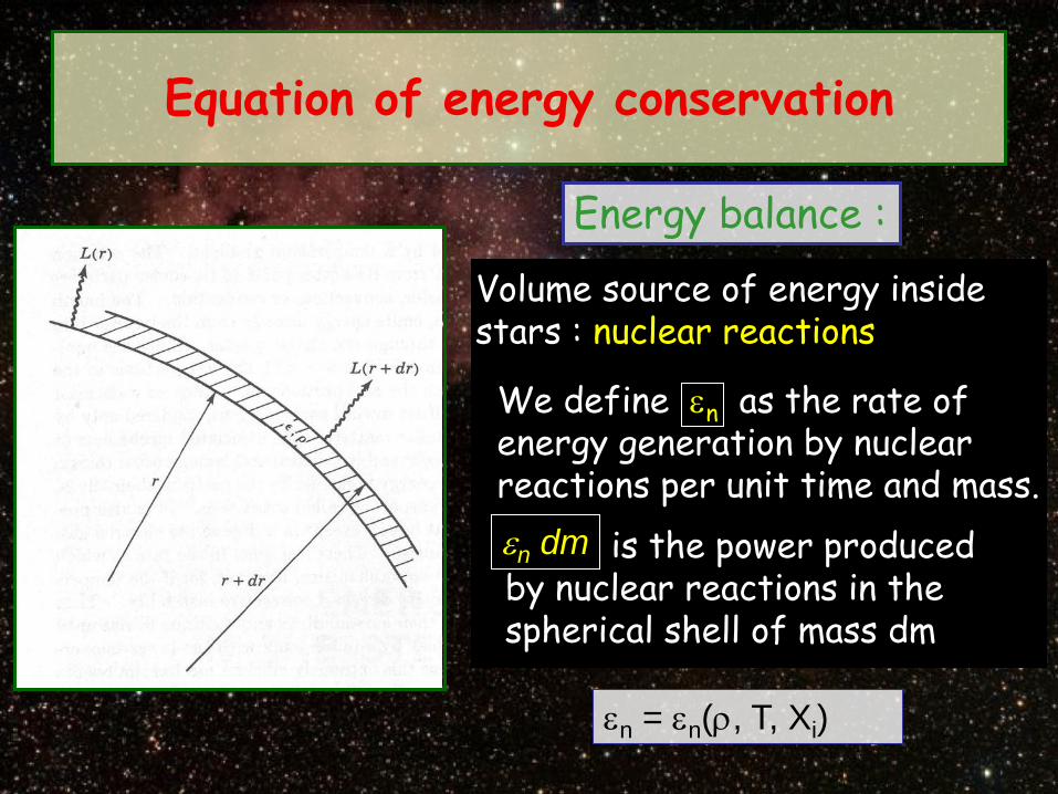
Energy balance :
Equation of energy conservation
Volume source of energy inside stars : nuclear reactions
εn = εn(ρ, T, Xi)
is the power produced by nuclear reactions in the spherical shell of mass dm
εn dm
We define εn as the rate of energy generation by nuclear reactions per unit time and mass.

Energy lost by the spherical shell per unit time:
L(r+dr) – L(r) = dL = ∂ L/∂ r dr
dL = εn dm ) d L/d m = εn
At thermal equilibrium: produced energy = lost energy
) dL/dr = 4π r2 ρ εn
Equation of energy conservation
Energy balance :

dtdsT
dmdL
n −= ε
dmdtdsTdm
dtdvP
dtdu
dmdtdQdLdm
- n
=
+ =
=ε
Out of thermal equilibrium
εgrav « Energy supply from the gravitational contraction » (see the Virial theorem)
Expansion power
Internal energy variation
Equation of energy conservation
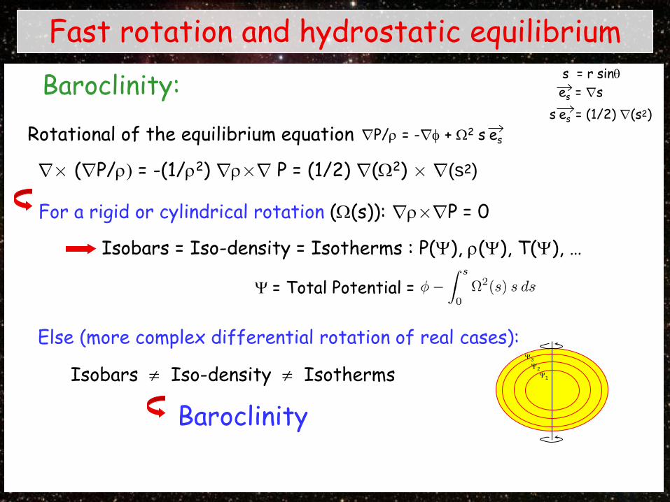
Baroclinity:
r£ (rP/ρ) = -(1/ρ2) rρ£r P = (1/2) r(Ω2) £ r(s2)
Rotational of the equilibrium equation rP/ρ = -rφ + Ω2 s es
s es = (1/2) r(s2)
For a rigid or cylindrical rotation (Ω(s)): rρ£rP = 0
Isobars = Iso-density = Isotherms : P(Ψ), ρ(Ψ), T(Ψ), …
Ψ = Total Potential =
Ψ1
Ψ2
Ψ3
Else (more complex differential rotation of real cases):
Isobars ≠ Iso-density ≠ Isotherms
Baroclinity
Fast rotation and hydrostatic equilibrium
s = r sinθ es = rs
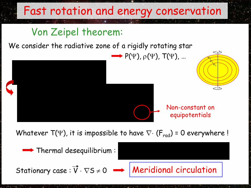
Fast rotation and energy conservation
Von Zeipel theorem: We consider the radiative zone of a rigidly rotating star P(Ψ), ρ(Ψ), T(Ψ), …
Ψ1
Ψ2
Ψ3
Non-constant on equipotentials
Whatever T(Ψ), it is impossible to have r¢ (Frad) = 0 everywhere !
Thermal desequilibrium :
Stationary case : V ¢ rS ≠ 0 Meridional circulation
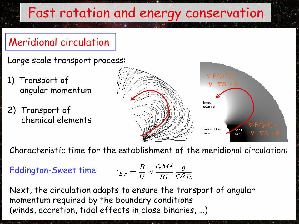
Large scale transport process: 1) Transport of angular momentum
2) Transport of chemical elements
Characteristic time for the establishment of the meridional circulation: Eddington-Sweet time: Next, the circulation adapts to ensure the transport of angular momentum required by the boundary conditions (winds, accretion, tidal effects in close binaries, …)
r¢F/(ρT) = - V ¢ rS < 0
r¢F/(ρT) = - V ¢ rS > 0
Fast rotation and energy conservation
Meridional circulation

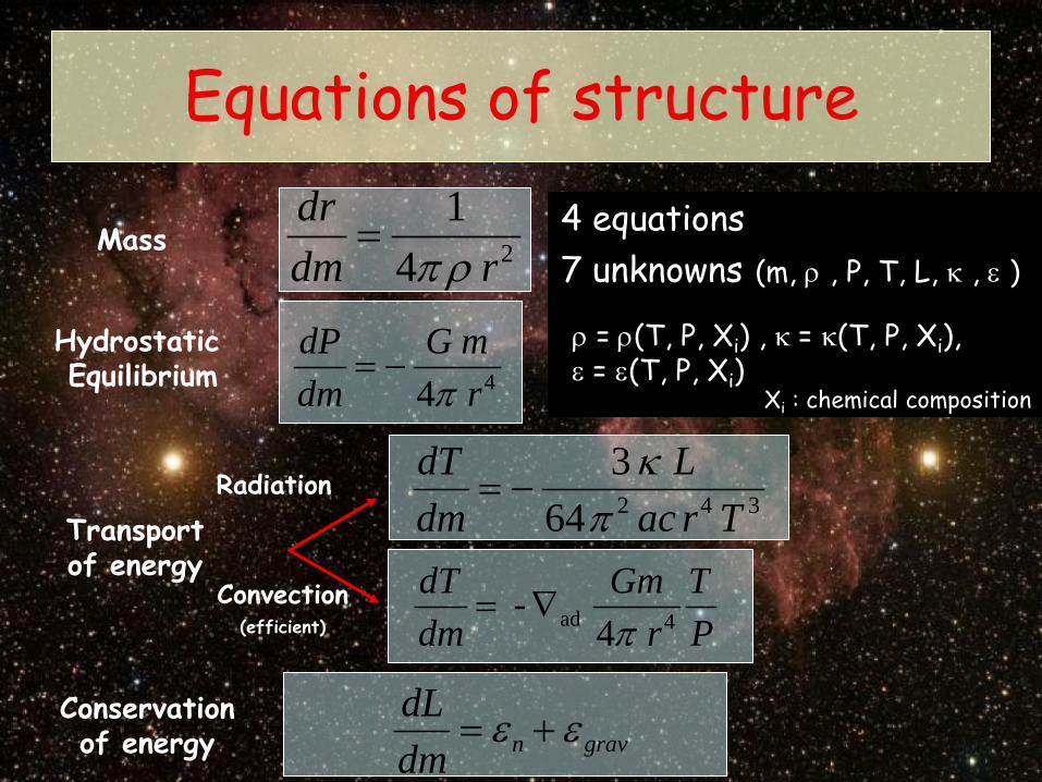
Equations of structure
24 rdrdm ρπ=Mass
2rmG
drdP ρ
−=Hydrostatic Equilibrium
32163
TracL
drdT
πρκ
−=Radiation
PT
rGm
drdT
2ad- ρ∇=
Transport of energy
)(4 2gravnr
drdL εερπ +=Conservation
of energy
4 equations 7 unknowns (m, ρ , P, T, L, κ , ε )
ρ = ρ(T, P, Xi) , κ = κ(T, P, Xi), ε = ε(T, P, Xi)
Xi : chemical composition
Convection (efficient)
241
rdmdr
ρπ=
4 4 rmG
dmdP
π−=
342643
TracL
dmdT
πκ
−=
PT
rGm
dmdT
4ad 4 -
π∇=
gravndmdL εε +=
Equations of structure
Mass
Hydrostatic Equilibrium
Radiation
Convection (efficient)
Transport of energy
Conservation of energy
4 equations 7 unknowns (m, ρ , P, T, L, κ , ε )
ρ = ρ(T, P, Xi) , κ = κ(T, P, Xi), ε = ε(T, P, Xi)
Xi : chemical composition
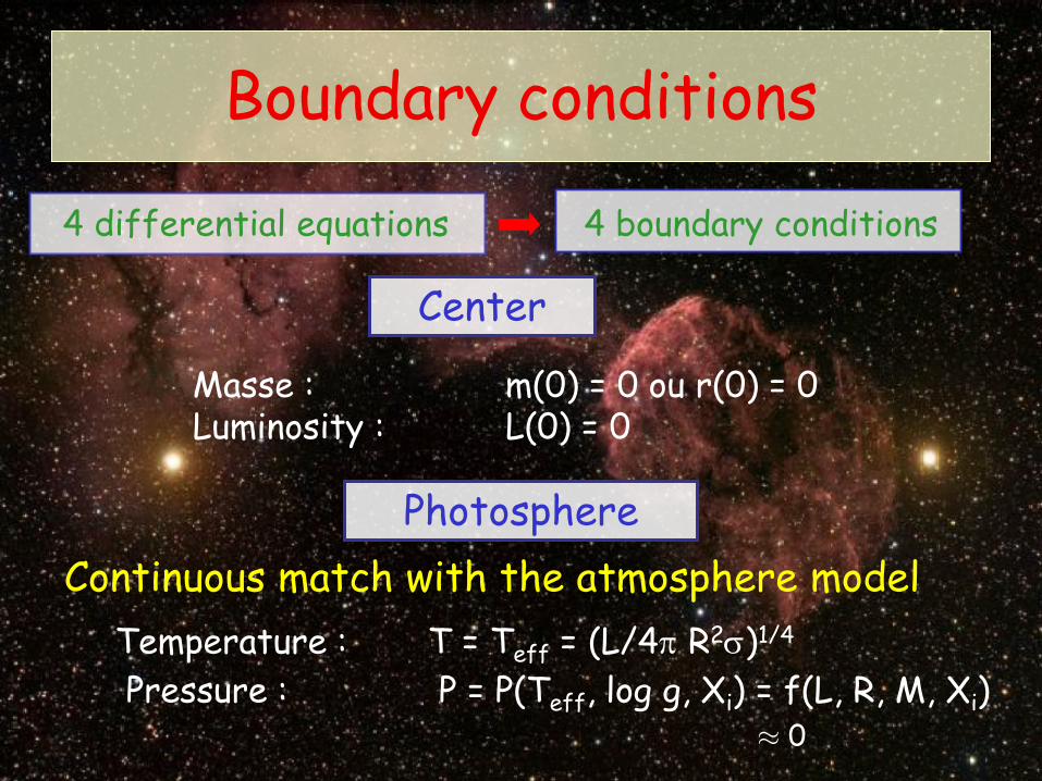
Boundary conditions
4 differential equations 4 boundary conditions
Masse : m(0) = 0 ou r(0) = 0 Luminosity : L(0) = 0
Center
Photosphere Continuous match with the atmosphere model
Temperature : T = Teff = (L/4π R2σ)1/4 Pressure : P = P(Teff, log g, Xi) = f(L, R, M, Xi)
¼ 0

State equation and chemical composition
Stars are mainly composed of: - Hydrogen (initial mass fraction X ~ 0.7) - Helium (initial mass fraction Y ~ 0.28) - Heavy elements (« metals »: Fe, C, N, O, …) total mass fraction Z ~ 0.015 for the Sun)
~ Perfect gas
The gas is nearly fully ionized in the stellar interior but Coulombian interaction between ions and electrons does not affect significantly their trajectories: (3/2) kT = Ekin > e2/d (electrostatic potential energy)

ugaz m
Tkk TnPµ
ρ ==Perfect gas Mean molecular weight (dimensionless)
n = ne + ∑i ni = ∑i (1+Zi)ni
Mixing of free electrons and nuclei
(fully ionized case)
Pgaz = Pe + ∑i Pi
ni = ρi/(Αi mu) = ρ Xi /(Αi mu)
µ = ( ∑i Xi (1+Zi) / Αi )-1
Equation of State

Pressure = normal momentum flux
Pressure integral
θ
All particles in the same direction :
Isotropic gas: Fraction of particles with direction between θ and θ+dθ :
Pressure of particles with angles in [θ, θ+dθ ] and momentum in [p, p+dp] :
Total pressure:
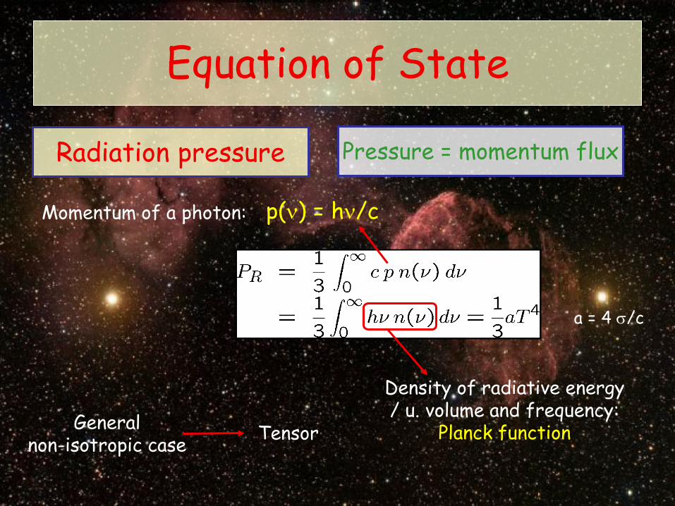
p(ν) = hν/c Momentum of a photon:
Radiation pressure
General non-isotropic case Tensor
Density of radiative energy / u. volume and frequency:
Planck function
Pressure = momentum flux
Equation of State
a = 4 σ/c

Total pressure 4
31 aTm
TkPu
+= µρ
In « hot » stars, PR = (1/3) aT4 can become significant
compared to Pgaz.
Equation of State

Total pressure 4
31 aTm
TkPu
+= µρ
But, gas of fermions
Pauli exclusion principle
Not more than 2 fermions in the phase volume: dpxdpydpz
dx dy dz = h3
Equation of State

Volume occupied in the phase space:
Equation of State
Quantum degeneracy of the electron gas
Maxwell-Boltzmann distribution
of momentum :
Number of electrons

Volume occupé dans l’espace des phases:
4π p2 dp dV
Equation of State
Quantum degeneracy of the electron gas
Volume occupied in the phase space:
Maxwell-Boltzmann distribution
of momentum :
Number of electrons

Degeneracy appears when ρ or T
Fermi-Dirac statistics
Equation of State
Quantum degeneracy of the electron gas
Maxwell-Boltzmann distribution
of momentum :

Degeneracy criterion
Equation of State
Quantum degeneracy of the electron gas
No degeneracy if
Mean molecular weight / electron
The degeneracy appears first for the electrons

Equation of State
Quantum degeneracy of the electron gas
A simple example: completely degenerated gas
(T ! 0 limit)
Fermi momentum
n
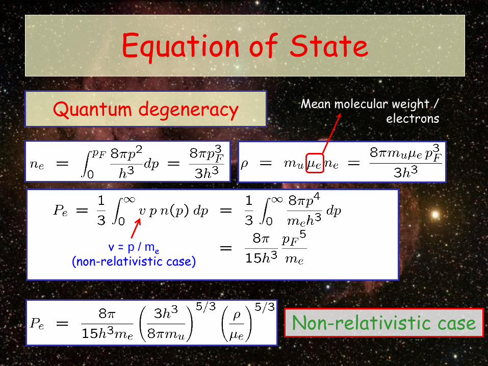
Quantum degeneracy
Non-relativistic case
Mean molecular weight / electrons
Equation of State
v = p / me (non-relativistic case)

Quantum degeneracy Mean molecular weight /
electrons
Equation of State
v ~ c (relativistic case)
Extremely relativistic case
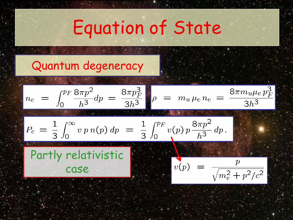
Partly relativistic case
Equation of State
Quantum degeneracy

Calculus of the electronic density and the mean molecular weight per electron
ni = ρi/(Αi mu) = ρ Xi /(Αi mu)
µe = ( ∑i Xi Zi / Αi )-1
Hydrogen (X), Helium (Y), metals (for the metals, Zi/Αi ' ½)
Equation of State
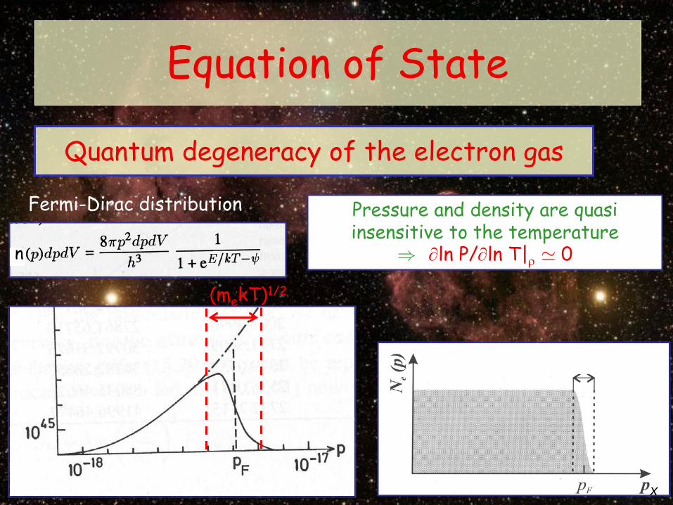
Pressure and density are quasi insensitive to the temperature
) ∂ln P/∂ln T|ρ ' 0
Fermi-Dirac distribution
x
(mekT)1/2
Equation of State
Quantum degeneracy of the electron gas
n

Radiation pressure:
ugR m
TkPaTPµ
ρ=≥= 4
31
Degeneracy:
(MKSA)
Relativistic degeneracy: Crystalisation
of ions
(g/cm3)
Equation of State

4
31 aTm
TkPu
+= µρ
Degenerated :
3/5)(e
eKP µ
ρ≈ 3/4)(e
eKP µ
ρ∗≈
Non-relativistic degeneracy Relativistic degeneracy
Non-degenerated :
Equation of State

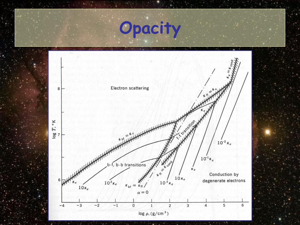
Opacity
Mean Rosseland opacity
32163
TracL
drdT
πρκ
−=
Parts of the spectrum which have the highest weight: - Maximum of the Planck distribution : ν ¼ kT/h - Less opaque regions (harmonic mean)
κ = κ(T, ρ, Xi) κν = f(ν, T, ρ, Xi)
Depends on the frequency

Planck function (Black body)
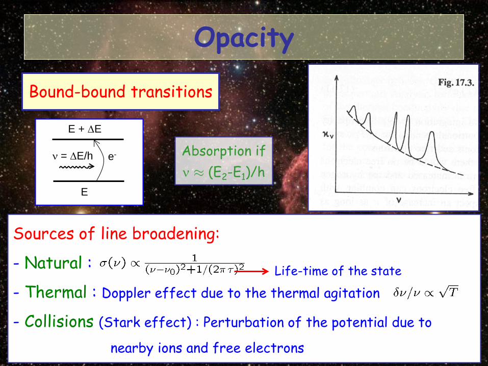
Opacity
Bound-bound transitions
Sources of line broadening:
- Natural :
- Thermal : Doppler effect due to the thermal agitation
- Collisions (Stark effect) : Perturbation of the potential due to
nearby ions and free electrons
Life-time of the state
Absorption if ν ¼ (E2-E1)/h
ν = ∆E/h
E
E + ∆E
e-

Opacity
Bound-bound transitions ν = ∆E/h
E
E + ∆E
e-
Calculation of the opacity : Nbr / m3
Cross-section of one transition
- Cross section determination for all transitions ! …
- Determination of the occupation of all electronic states
Cross section: σν n = κν ρ = Σi,j ni σν i,j
T < 106 K up to 50% T ~ 107 K less than 10%
Contribution of the bound-bound transitions to the total opacity :
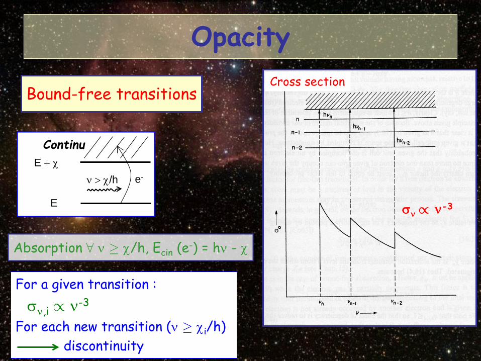
Bound-free transitions
Absorption 8 ν ¸ χ/h, Ecin (e-) = hν - χ
σν / ν-3
For a given transition : σν,i / ν-3 For each new transition (ν ¸ χi/h) discontinuity
Cross section
Opacity
ν > χ/h
E
E + χ
e-
Continu
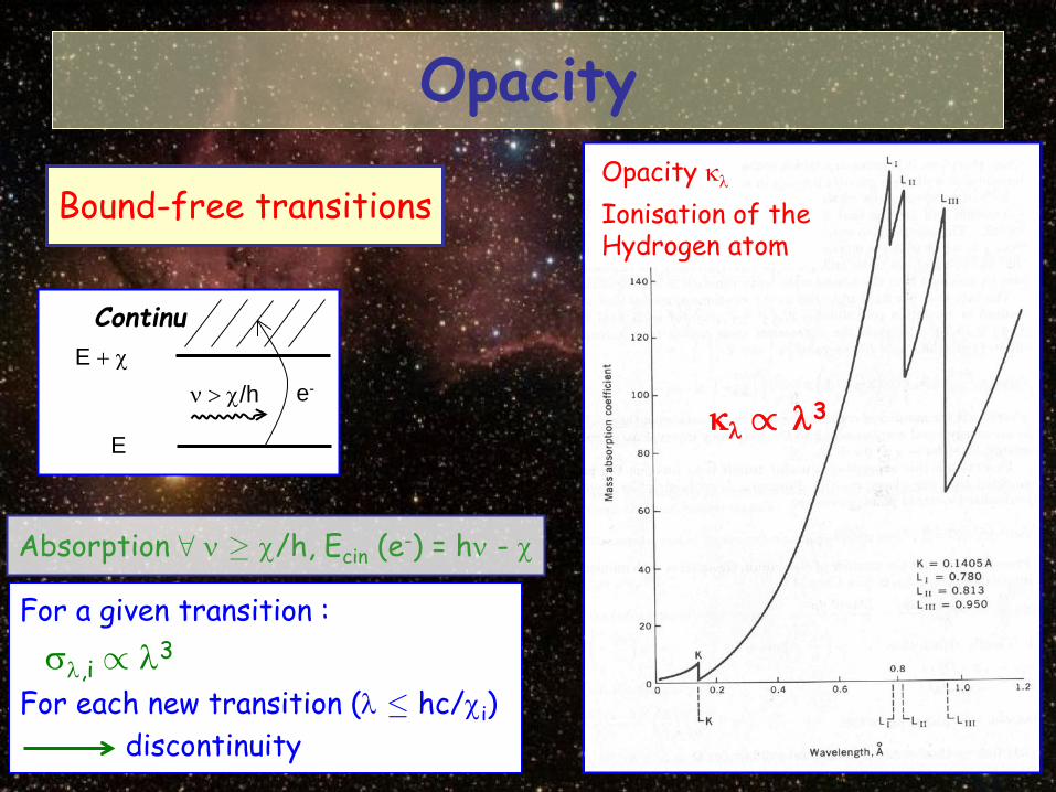
Absorption 8 ν ¸ χ/h, Ecin (e-) = hν - χ
κλ / λ3
For a given transition : σλ,i / λ3 For each new transition (λ · hc/χi) discontinuity
Ionisation of the Hydrogen atom
Opacity κλ
Opacity
Bound-free transitions
ν > χ/h
E
E + χ
e-
Continu

Grosso-modo … At a given temperature : hν ~ kT
Opacity calculation : - Cross section determination for all possible ionizations …
- Determination of the occupation of all electronic states :
free electrons, states of ionisation (Saha eq.) and excitation (Boltzmann)
Transitions with χi >> kT never occur because too few photons have enough energy Transitions with χi << kT never occur because too few ions are at the required initial ionization state (Saha)
transitions with χi ' kT occur
Absorption 8 ν ¸ χ/h, Ecin (e-) = hν - χ
Opacity
Bound-free transitions

Absorption 8 ν ¸ χ/h
Total opacity : complicated !
Opacity
Bound-free transitions
ν > χ/h
E
E + χ
e-
Continu
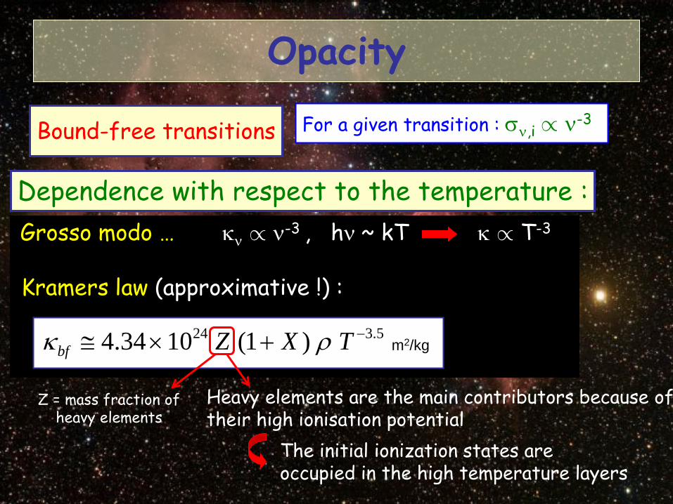
For a given transition : σν,i / ν-3
Dependence with respect to the temperature : Grosso modo … κν / ν-3 , hν ~ kT κ / T-3
Kramers law (approximative !) :
5.324 )1(1034.4 −+×≅ TXZbf ρκ
Heavy elements are the main contributors because of their high ionisation potential
The initial ionization states are occupied in the high temperature layers
Z = mass fraction of heavy elements
m2/kg
Opacity
Bound-free transitions

Free-free absorptions
E cin, fin(e-) = E cin, init(e-) + hν
hν e-
Z
e- An ion is needed to ensure the momentum conservation
5.321 )1()(1068.3 −++≅ TXYXff ρκ
Kramers law(approx.)
σλ / λ3/v
Initial velocity of the electron
λ ~ hc/(kT)
v ~ (3kT/me)1/2
κ / T-3.5
Inverse Bremsstrahlung
Limitation: Degenerated gas
High number of impossible transitions (many occupied states)
Smaller opacity
m2/kg
Opacity
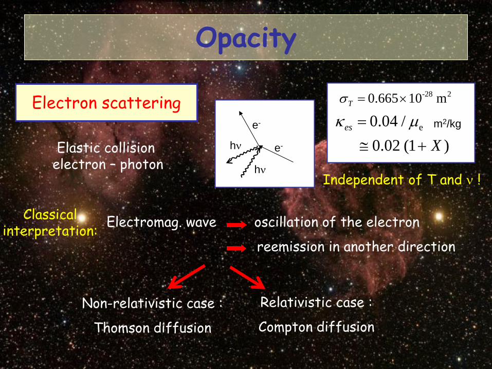
)1(02.0 / 0.04 e
Xes
+≅= µκ
Electron scattering
hν e-
e-
hν
Elastic collision electron – photon
Non-relativistic case :
Thomson diffusion
Relativistic case :
Compton diffusion
Electromag. wave oscillation of the electron
reemission in another direction
Classical interpretation:
Independent of T and ν !
2-28 m 10 0.665 ×=Tσ
m2/kg
Opacity

Bound-Free transitions
Free-Free transitions
Approximation Kramers laws
5.324 )1(1034.4 −+≅ TXZbf ρκ
5.321 )1()(1068.3 −++≅ TXYXff ρκ
Electron scattering )1(02.0 Xes +≅κ
Bound-Bound transitions
m2/kg
m2/kg
m2/kg
In the 3 last cases: κ / nbr. e-/m3 / 1+X
Opacity

Electronic conduction
If the electron gas is highly degenerated
Very high kinetic energy of the electrons
They efficiently transport energy by conduction
« As if the opacity was lower »
Opacity
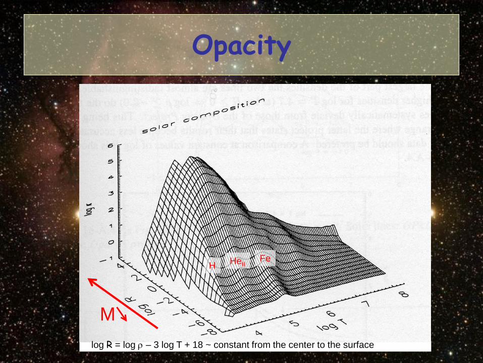
Opacity
M
HeII Fe H
log R = log ρ – 3 log T + 18 ~ constant from the center to the surface
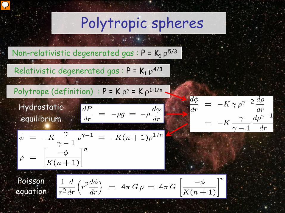
Polytropic spheres
Non-relativistic degenerated gas : P = K1 ρ5/3
Relativistic degenerated gas : P = K1 ρ4/3
Polytrope (definition) : P = K ργ = K ρ1+1/n
Hydrostatic equilibrium
Poisson
equation
Presenter
Presentation Notes
short-circuit
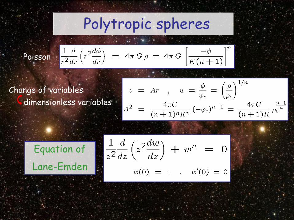
Poisson
Change of variables dimensionless variables
Equation of
Lane-Emden
Polytropic spheres

Cases with analytical solutions :
Equation de
Lane-Emden
Other important cases: n = 3/2 (γ = 5/3, non-relativistic degenerated)
n = 3 (γ = 4/3, relativistic degenerated) n = 1 (γ = 1, isothermal sphere, infinite radius)
n < 5 ( γ > 6/5 ) Finite radius, n ¸ 5 Infinite radius
Polytropic spheres
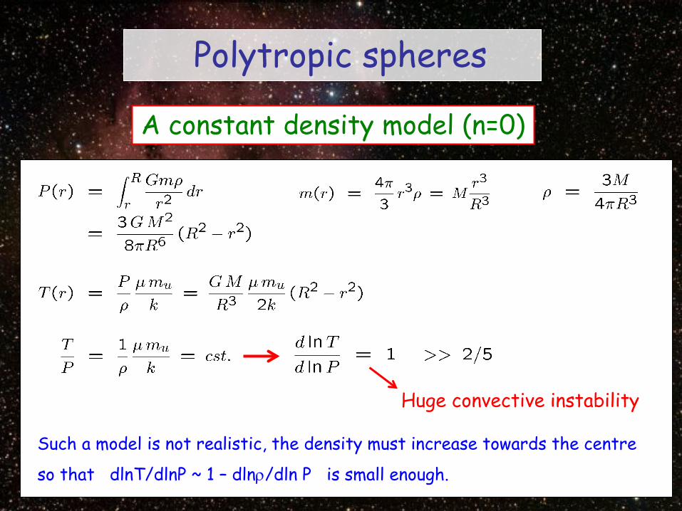
A constant density model (n=0)
Huge convective instability
Such a model is not realistic, the density must increase towards the centre
so that dlnT/dlnP ~ 1 – dlnρ/dln P is small enough.
Polytropic spheres
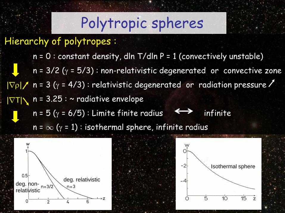
Hierarchy of polytropes : n = 0 : constant density, dln T/dln P = 1 (convectively unstable)
n = 3/2 (γ = 5/3) : non-relativistic degenerated or convective zone
n = 3 (γ = 4/3) : relativistic degenerated or radiation pressure
n = 3.25 : ~ radiative envelope
n = 5 (γ = 6/5) : Limite finite radius infinite n = 1 (γ = 1) : isothermal sphere, infinite radius
|rρ| |rT|
deg. relativistic deg. non- relativistic
Isothermal sphere
Polytropic spheres

Un modèle simple d’enveloppe radiative
Kramers : a = 1 , b = -4.5
Hypothèses:
- Enveloppe radiative :
- Opacités : - L, m constants (ε = 0, ρ petit)
Polytrope n = 3.25

Mass
Mass-radius relation of polytropes
Polytropic spheres
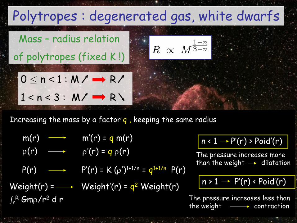
Mass – radius relation
of polytropes (fixed K !)
Polytropes : degenerated gas, white dwarfs
0 · n < 1 : M R
1 < n < 3 : M R
m(r) m’(r) = q m(r)
ρ(r) ρ’(r) = q ρ(r)
Weight(r) = Weight’(r) = q2 Weight(r) sr
R Gmρ/r2 d r
P(r) P’(r) = K (ρ’)1+1/n = q1+1/n P(r)
n < 1 P’(r) > Poid’(r)
Increasing the mass by a factor q , keeping the same radius
The pressure increases more than the weight dilatation
n > 1 P’(r) < Poid’(r)
The pressure increases less than the weight contraction

Mass - Radius relation of polytropes (fixed K)
Non-relativistic degenerated gas, n = 3/2 :
Polytropes : degenerated gas, white dwarfs
Relativistic degenerated gas, n = 3 : M = Constant !
Chandrasekhar’s limiting mass
When the state of matter tends towards complete non-rel. degeneracy:
R ~ constant Cooling at constant radius of white dwarfs
Presenter
Presentation Notes
Subrahmanyan Chandrasekhar est un astrophysicien et un mathématicien d'origine indienne. Il est lauréat du prix Nobel de physique de 1983. (19 octobre 1910 à Lahore, Punjab, Indes britanniques - 21 août 1995 à Chicago).
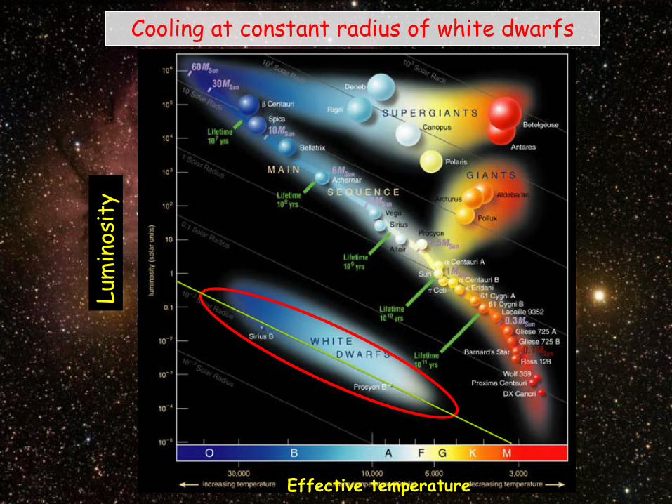
Lum
inos
ity
Effective temperature
Cooling at constant radius of white dwarfs
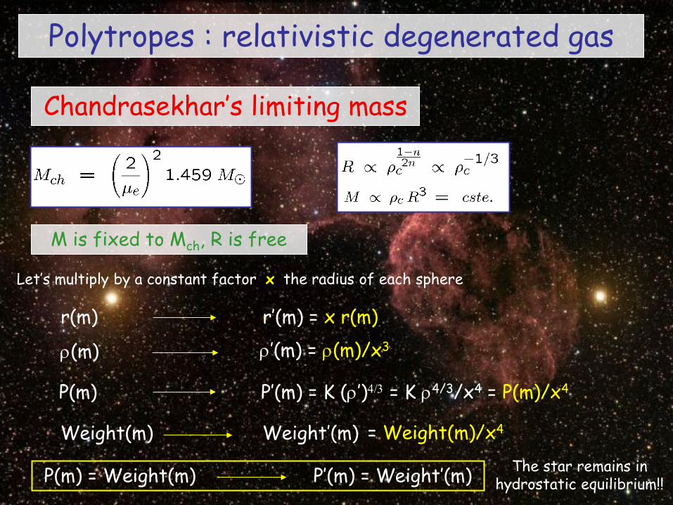
Chandrasekhar’s limiting mass
M is fixed to Mch, R is free
r(m) r’(m) = x r(m)
ρ(m) ρ’(m) = ρ(m)/x3
Weight(m) Weight’(m) = Weight(m)/x4
P(m) P’(m) = K (ρ’)4/3 = K ρ4/3/x4 = P(m)/x4
P(m) = Weight(m) P’(m) = Weight’(m)
Polytropes : relativistic degenerated gas
Let’s multiply by a constant factor x the radius of each sphere
The star remains in hydrostatic equilibrium!!

What happens when M > Mch ?
r(m) r’(m) = x r(m)
ρ(m) ρ’(m) = ρ(m)/x3
Weight(m) Weight’(m) = Weight(m)/x4
P(m) P’(m) = P(m)/x4
P’(m) < Poid’(m) The collapse continues
P(m) < Poids(m) contraction
No hydrostatic equilibrium
Chandrasekhar’s limiting mass
Polytropes : relativistic degenerated gas
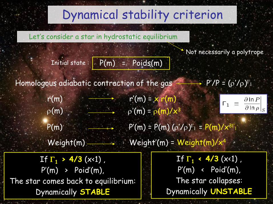
Let’s consider a star in hydrostatic equilibrium
r(m) r’(m) = x r(m)
ρ(m) ρ’(m) = ρ(m)/x3
Weight(m) Weight’(m) = Weight(m)/x4
P(m) P’(m) = P(m) (ρ’/ρ)Γ1 = P(m)/x3Γ1
If Γ1 > 4/3 (x<1) , P’(m) > Poid’(m),
The star comes back to equilibrium: Dynamically STABLE
P(m) = Poids(m)
Dynamical stability criterion
Not necessarily a polytrope
Initial state :
Homologous adiabatic contraction of the gas P’/P = (ρ’/ρ)Γ1
If Γ1 < 4/3 (x<1) , P’(m) < Poid’(m), The star collapses:
Dynamically UNSTABLE
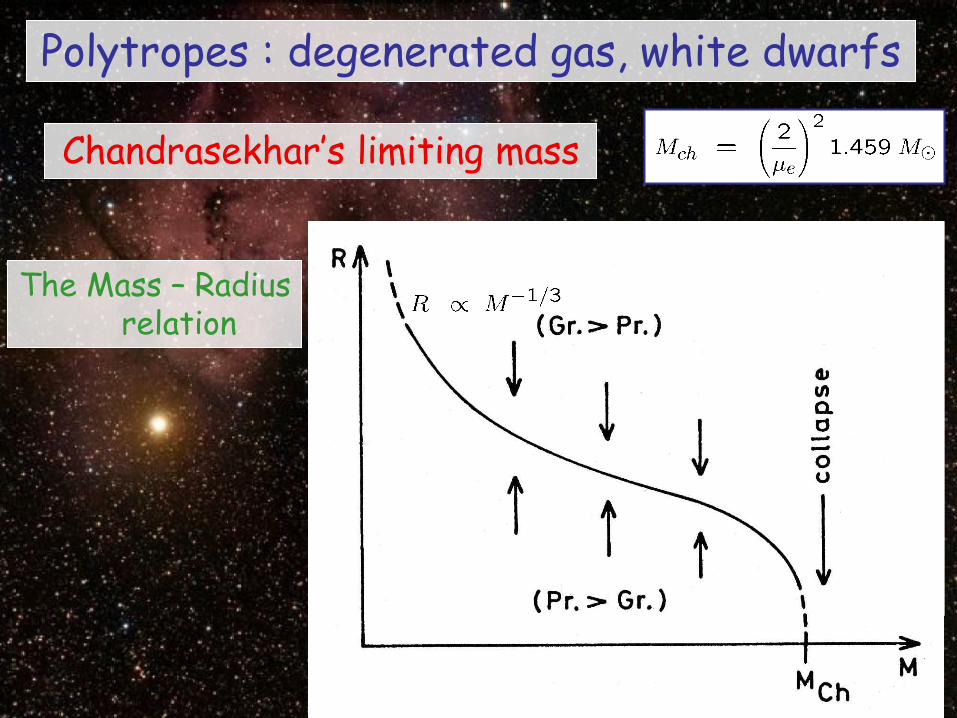
The Mass – Radius relation
Chandrasekhar’s limiting mass
Polytropes : degenerated gas, white dwarfs

slowly accretes matter from its red giant companion
1st scenario (the most frequent): White dwarf of C-O in a binary system
What happens when the Chandrasekhar’s limiting mass is reached ?
The C-O core’s mass reaches the Chandrasekhar’s limit !
the C-O core’s mass increases
2nd scenario : During shell burning of H and He,
The core contracts and reaches huge densities
Nuclear reactions in a degenerated medium thermal runaway The entire star burns and explodes like a huge thermonuclear bomb.
Type Ia supernova L ~ 109 - 1010 L¯
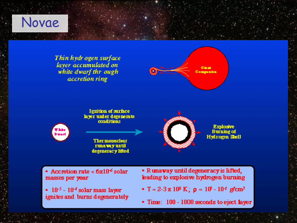
Novae
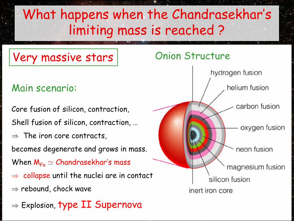
Very massive stars
Main scenario:
Core fusion of silicon, contraction,
Shell fusion of silicon, contraction, …
) The iron core contracts,
becomes degenerate and grows in mass.
When MFe ' Chandrasekhar’s mass
) collapse until the nuclei are in contact
) rebound, chock wave
) Explosion, type II Supernova
Onion Structure
What happens when the Chandrasekhar’s limiting mass is reached ?
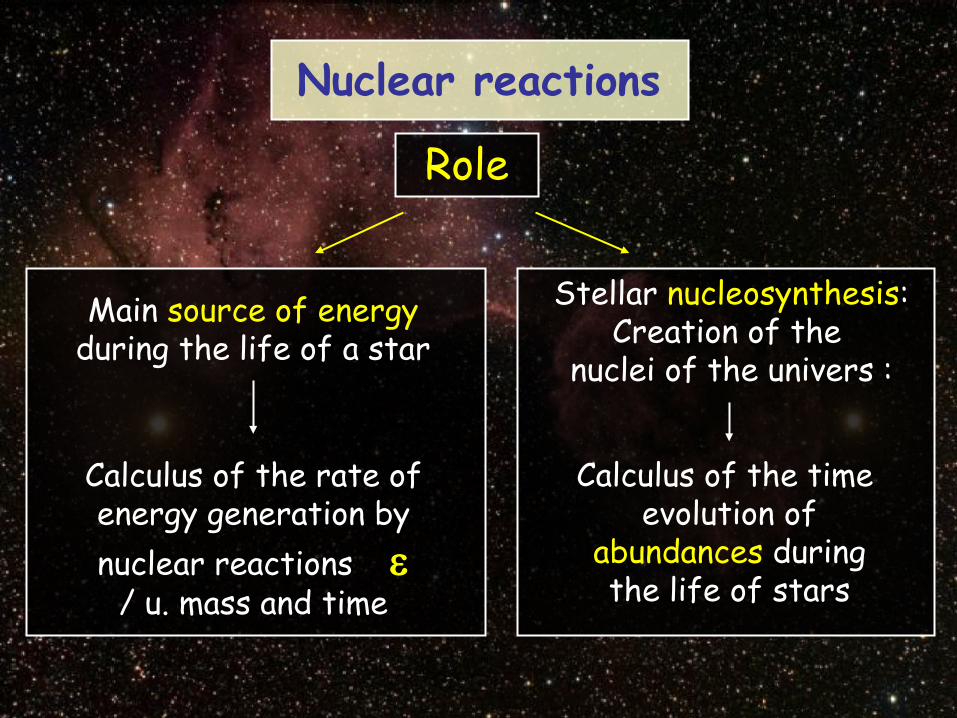
Nuclear reactions
Main source of energy during the life of a star
Role
Calculus of the rate of energy generation by nuclear reactions ε
/ u. mass and time
Stellar nucleosynthesis: Creation of the
nuclei of the univers :
Calculus of the time evolution of
abundances during the life of stars

• Momentum conservation
Movement eq. of the “relative particle” in a fixed potential :
Classical (Newton):
Quantum (Schroedinger) :
Conservation laws
Reduced mass
(2 bodies problem, non-relativistic)
• Charge conservation
• Nuclei conservation
Nuclear reactions
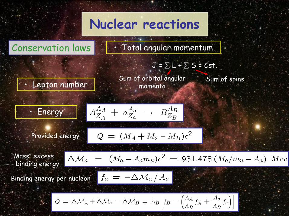
• Total angular momentum
J = ∑ L + ∑ S = Cst.
“Mass” excess = - binding energy
Sum of spins
• Energy
Sum of orbital angular momenta
Provided energy
• Lepton number
Binding energy per nucleon
Nuclear reactions
Conservation laws

• Energy
Provided energy Binding energy / nucleon

Reaction rate = nbr. of reactions
/ u. time and volume
Nbr. of particle couples
/ u. volume2 Relative speed
Cross section
Speed distribution
Rate of energy generation ε = power / u. mass
Sum over all reactions
Nuclear reactions

Total kinetic energy in the center of mass frame:
Probability density of E : (Boltzmann, Fermi-Dirac, …)
The whole difficulty is the determination of the cross section σ(E)
Nuclear reactions
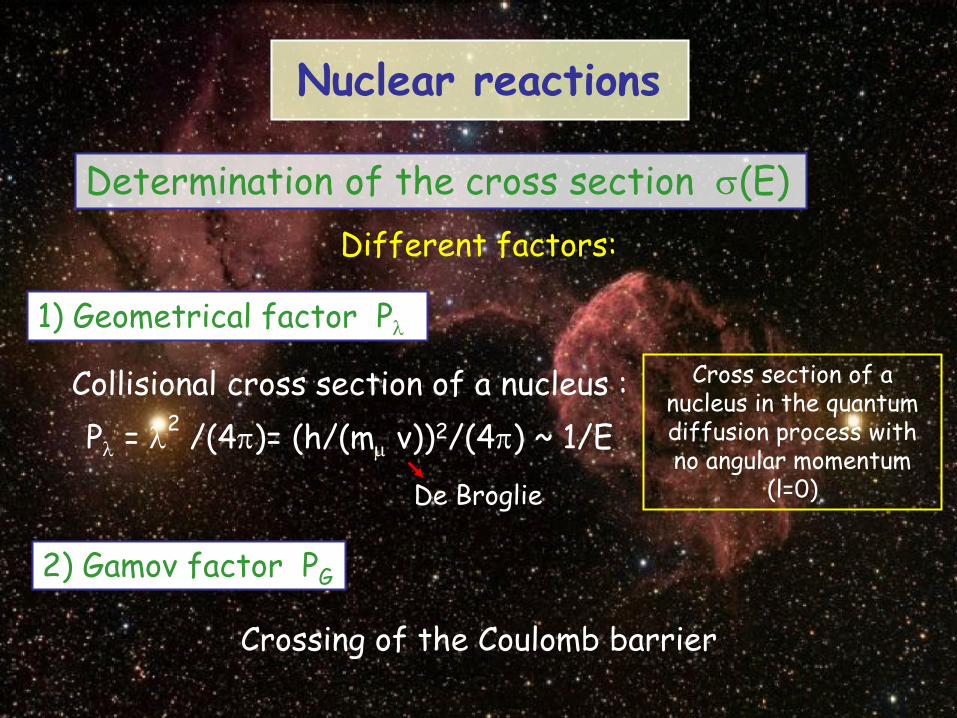
Determination of the cross section σ(E) Different factors:
1) Geometrical factor Pλ
Collisional cross section of a nucleus : Pλ = λ2 /(4π)= (h/(mµ v))2/(4π) ~ 1/E
De Broglie
2) Gamov factor PG
Crossing of the Coulomb barrier
Cross section of a nucleus in the quantum diffusion process with no angular momentum
(l=0)
Nuclear reactions

The Coulomb barrier
for T ~ 107 K
r0 : nuclear radius
More than 1000 times too small
Probability e-1000 (Max-Boltz.) !
Impossible
ECb
rmin
Nuclear reactions
Determination of the cross section σ(E)
2) Gamov factor PG
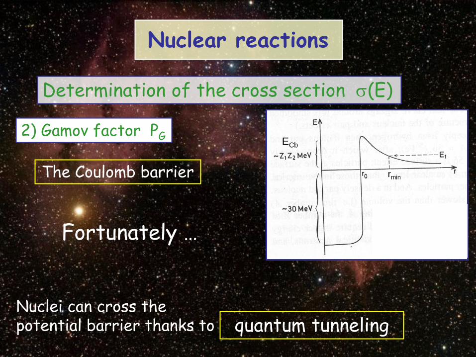
Fortunately …
quantum tunneling Nuclei can cross the potential barrier thanks to
ECb
rmin
Nuclear reactions
The Coulomb barrier
2) Gamov factor PG
Determination of the cross section σ(E)

Wave function :
Schroedinger eq. :
Crossing probability of the Coulomb barrier
Square potential barrier
2) Gamov factor PG
Determination of the cross section σ(E)
Nuclear reactions

Quantum tunneling
Coulomb potential Crossing probability of the Coulomb
barrier (WKB approximation) :
ECb
rmin
Nuclear reactions
2) Gamov factor PG
Determination of the cross section σ(E)

Crossing probability of the Coulomb barrier (WKB approximation) :
ECb
rmin
Nuclear reactions
2) Gamov factor PG
Determination of the cross section σ(E)
Quantum tunneling
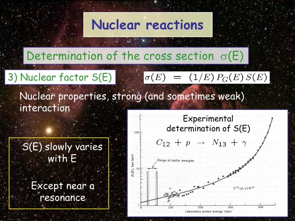
3) Nuclear factor S(E)
Nuclear properties, strong (and sometimes weak) interaction
S(E) slowly varies with E
Except near a resonance
Experimental determination of S(E)
Nuclear reactions
Determination of the cross section σ(E)

f
m
m
Nuclear reactions
Determination of the cross section σ(E)
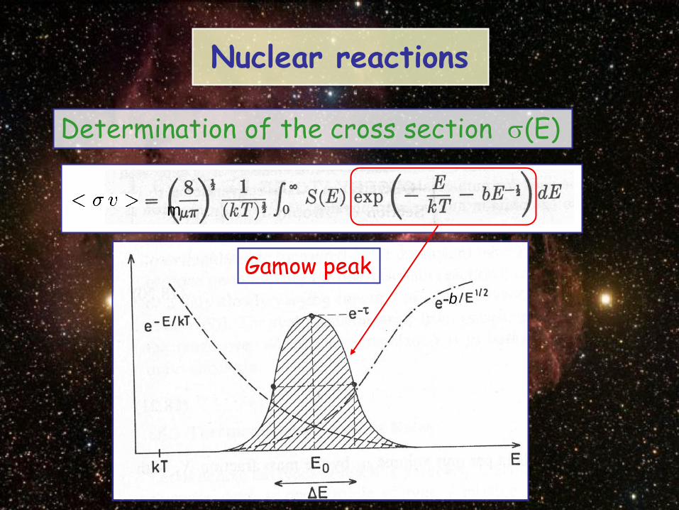
b
Gamow peak
m
Nuclear reactions
Determination of the cross section σ(E)

m
Nuclear reactions
Determination of the cross section σ(E)
Gamow peak
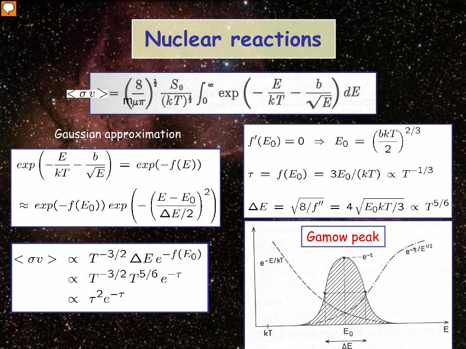
Gaussian approximation
m
Nuclear reactions
Gamow peak
Presenter
Presentation Notes
standard deviation Integral d’une gaussienne normalisée : racine(pi)

Light nuclei: ν ∼ 6 ( < σ v > / T6 )
Heavy nuclei:
ν ∼ 20-30 !! ( < σ v > / T30 )
Extremely sensitive to the temperature !!
T7 = T (K) / 107
Nuclear reactions

Resonant reactions
Discrete set of states-energies of the nuclei ~ electronic levels of atoms
Shell-model: Each nucleon in the average potential generated by the
others
Nuclear reactions
Presenter
Presentation Notes
This observation, that there are certain magic numbers of nucleons: 2, 8, 20, 28, 50, 82, 126 which are more tightly bound than the next higher number, is the origin of the shell model 82 : Plomb (lead=liiid)

Discrete set of states-energies of the nuclei ~ atoms
Quasi- stationary levels
Stationary levels
If E is near En
Resonant reaction
Nuclear reactions
Resonant reactions

Around the resonance energy:
For E ~ Eres , σ ∼ σmax = (2l+1) λ2 /(4π) = (2l+1) π (~/(mµ v))2
σ very high for the nuclei colliding with the required angular momentum and a near-resonance energy
S(E) is sharp around Eres
Γ
Even more sensitive to the temperature
ex : reaction 3α : ε ~ T40 !!!
Must remain inside the integral
Γ = ~/τ Nuclear reactions
Resonant reactions

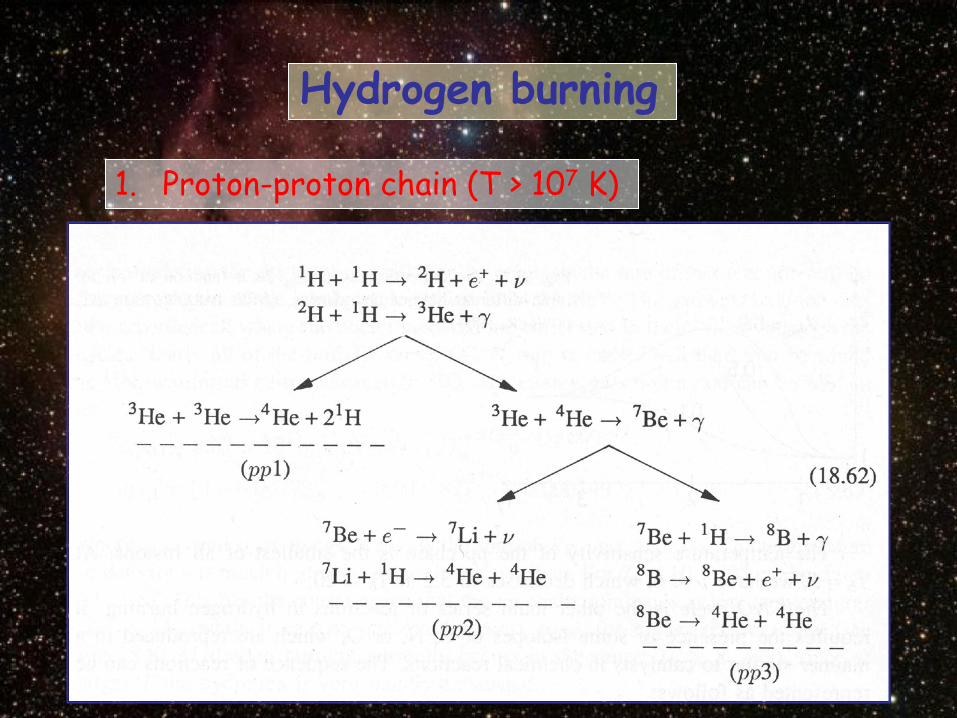
Hydrogen burning
1. Proton-proton chain (T > 107 K)
eeHHH ν++→+ 0
1
2
1
1
1
1
1
γ+→+ HeHH 32
21
11
HHeHeHe 11
42
32
32 2+→+
PPI
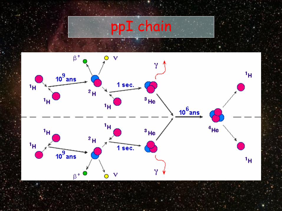
ppI chain
Hydrogen burning
1. Proton-proton chain (T > 107 K)

eeHHH ν++→+ 0
1
2
1
1
1
1
1
γ+→+ HeHH 32
21
11
HHeHeHe 11
42
32
32 2+→+
PPI
But : - Energy loss by neutrinos ! - Out of equilibrium !
Energy of the neutrino
Somme sur les réactions
4
Hydrogen burning
1. Proton-proton chain (T > 107 K)
Presenter
Presentation Notes
“Mass” excess
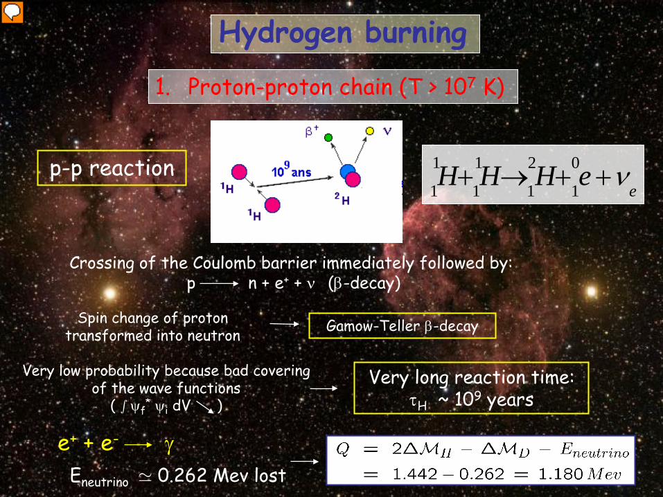
Crossing of the Coulomb barrier immediately followed by: p n + e+ + ν (β-decay)
Spin change of proton transformed into neutron Gamow-Teller β-decay
Very low probability because bad covering of the wave functions
( s ψf* ψi dV )
Very long reaction time: τH ~ 109 years
e+ + e- γ Eneutrino ' 0.262 Mev lost
eeHHH ν++→+ 0
1
2
1
1
1
1
1p-p reaction
1. Proton-proton chain (T > 107 K)
Hydrogen burning
Presenter
Presentation Notes
Discovered by Hans Bethe (1939)

Deuterium life-time:
τD ~ 1 sec. γ+→+ HeHH 32
21
11
Deuterium burning
In earth’s oceans: D/H = 1.5 £ 10-4
(Big-bang + solar heating of comets’ ice ?)
First: Burning of initial deuterium, next equilibrium.
1. Proton-proton chain (T > 107 K)
Hydrogen burning
Presenter
Presentation Notes
This is thought to be as a result of natural isotope separation processes that occur from solar heating of ices in comets. Like the water-cycle in Earth's weather, such heating processes may enrich deuterium with respect to protium. Kinetics -> kineeetiks

He3 + He3 reaction
Deuterium at equilibrium
HHeHeHe 11
42
32
32 2+→+
First, very slow reaction !!
Decreases as T
For too low T, He3 does not have time to reach equilibrium He3 peak
1. Proton-proton chain (T > 107 K)
Hydrogen burning

HHeHeHe 11
42
32
32 2+→+
Decreases as T
τeq (years)
Sun
m/M
1. Proton-proton chain
He3 + He3 reaction
Hydrogen burning
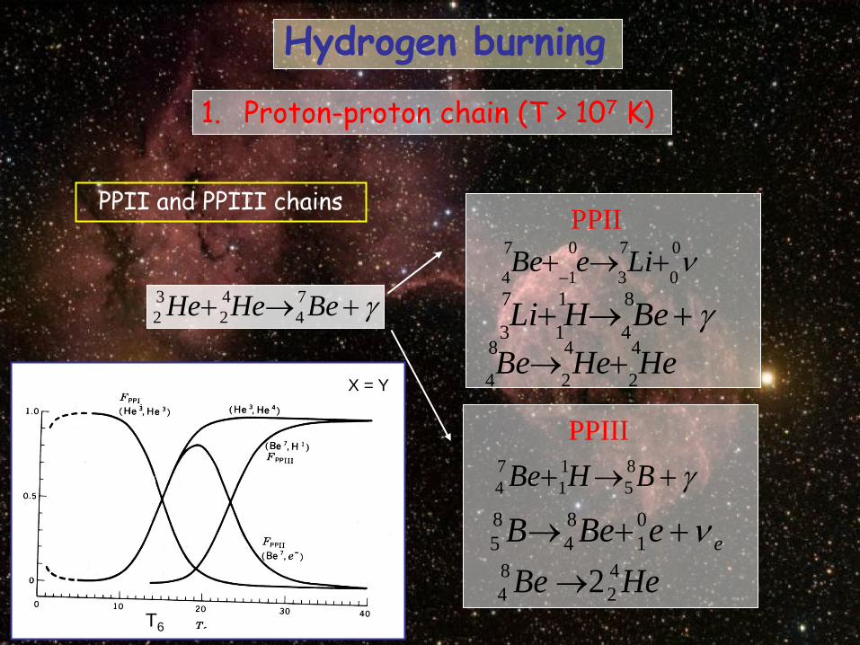
PPII and PPIII chains
γ+→+ BeHeHe 74
42
32
PPIII γ+→+ BHBe 8
511
74
eeBeB ν++→ 01
84
85
HeBe 42
84 2→
PPII ν0
0
7
3
0
1
7
4+→+
−LieBe
γ+→+ BeHLi 8
4
1
1
7
3
HeHeBe 4
2
4
2
8
4+→
T6
X = Y
Hydrogen burning
1. Proton-proton chain (T > 107 K)
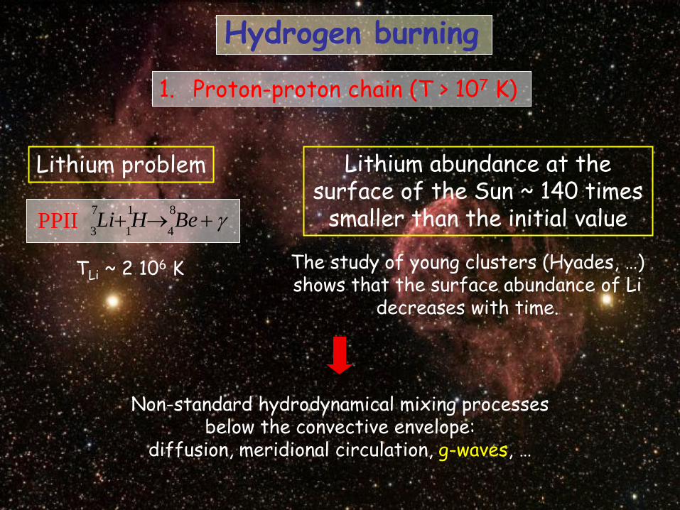
Lithium problem
Non-standard hydrodynamical mixing processes below the convective envelope:
diffusion, meridional circulation, g-waves, …
Lithium abundance at the surface of the Sun ~ 140 times
smaller than the initial value PPII γ+→+ BeHLi 8
4
1
1
7
3
The study of young clusters (Hyades, …) shows that the surface abundance of Li
decreases with time.
TLi ~ 2 106 K
Hydrogen burning
1. Proton-proton chain (T > 107 K)

Different energies of the neutrinos :
PPII ν00
7
3
0
1
7
4+→+
−LieBe
PPIII eeBeB ν++→ 01
84
85
PPI eeHHH ν++→+ 0
1
2
1
1
1
1
1
Eν = 0.263 Mev
Eν = 0.8 Mev
Eν = 7.2 Mev
Loss : 2 £ 0.263 = 2 %
Loss : 0.263 + 0.8 = 4 %
Loss : 0.263 + 7.2 = 27.9 %
26.73
26.73
26.73
Hydrogen burning
1. Proton-proton chain (T > 107 K)

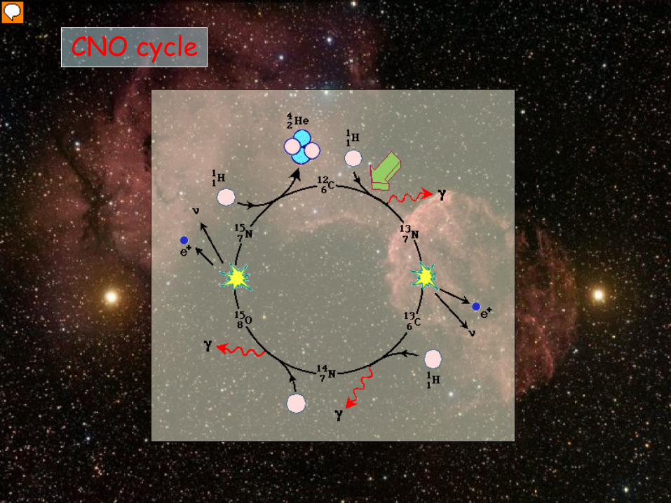
2. CNO cycle T > 17 x 106 K
Hydrogen burning
CNO cycle
Presenter
Presentation Notes
Catalyseur = catalyst

2. CNO cycle T > 17 x 106 K
γ+→+ OHN 15
8
1
1
14
7
Main loop :
Slowest reaction: At equilibrium, most of the C and O has been transformed
into 14N
Secondary loop
104 times less probable Main role: conversion O16 N14
Hydrogen burning
104 times less probable

1. C12 N14 O16 N14 (much slower)
2. Complex because : - Presence of a convective core which
homogenizes and of which mass is varying
- Some elements never reach the equilibrium value
Initially : C12 : N14 : O16 = 5.5 : 1 : 9.5
At equilibrium (typically) : C12 : N14 : O16 = 0.15 : 15 : 0.3
2. CNO cycle T > 17 x 106 K
Hydrogen burning

T15
T5 Log ε
T6
The CNO dominates for T > 17 £ 106 K
Massive stars
εpp / T5 εCNO / T15
2. CNO cycle T > 17 x 106 K
Hydrogen burning
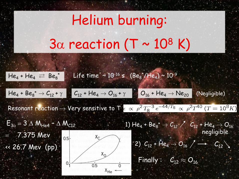
Helium burning:
3α reaction (T ~ 108 K)
He4 + He4 À Be8*
He4 + Be8* ! C12 + γ C12 + He4 ! O16 + γ O16 + He4 ! Ne20
Resonant reaction ! Very sensitive to T
Life time ~ 10-16 s (Be8*/He4) ~ 10-9
(Negligible)
C12 + He4 ! O16 negligible
2) C12 + He4 ! O16
1) He4 + Be8* ! C12
Finally : C12 ¼ O16
C12
E3α = 3 ∆ MHe4 – ∆ MC12
= 7.375 Mev
<< 26.7 Mev (pp)

α Captures
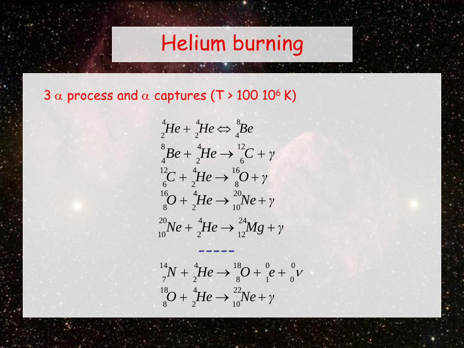
Helium burning
3 α process and α captures (T > 100 106 K)
γO HeC +→+ 16
8
4
2
12
6
γCHeBe +→+ 12
6
4
2
8
4
BeHeHe 8
4
4
2
4
2⇔+
ν00
0
1
18
8
4
2
14
7++→+ eO HeN
γNe HeO +→+ 20
10
4
2
16
8
γMg HeNe +→+ 24
12
4
2
20
10
γNe HeO +→+ 22
10
4
2
18
8
-----

Evolution: high masses Advanced phases of nuclear reactions
in high mass stars
HNaCC 1
1
23
12
12
6
12
6+→+
n Mg CC 1
0
23
12
12
6
12
6+→+
HeNeCC 4
2
20
10
12
6
12
6+→+
Q (Mev)
Carbon burning (T ~ 6-8 x 10⁸ K)
12C + 1H → 13N + γ 13N → 13C + e+ + ν 13C + 4He → 16O + 1n
Source of neutrons
<Q> ~ 13 Mev εcc / exp(-84/T9
1/3)

Photo-disintegration of neon (T ~ 1.2-1.5 x 10⁹ K) HeOγNe 4
2168
*2010 Ne +→→+ kT ~ 0.12 MeV Q = 4.73 Mev
« Thermodynamic » equilibrium
As much reactions in each sense ! reaction rate :
T % ) equilibrium towards more de photo-disintegration
~ Saha
The liberated α nuclei are immediately captured:
MgNe 2412
42
2010 He →+ Mev4.58 O 2 24
1216
82010 ++→ MgNe)
Advanced phases of nuclear reactions
in high mass stars

Oxygen burning (T ~ 2 x 10⁹ K)
Q (Mev)
For example …
<Q> ~ 16 Mev
Final product: 2/3 of 28Si for 1/3 of 32S
Advanced phases of nuclear reactions
in high mass stars

Q (Mev)
Advanced phases of nuclear reactions
in high mass stars
Oxygen burning (T ~ 2 x 10⁹ K)
<Q> ~ 16 Mev
Final product: 2/3 of 28Si for 1/3 of 32S
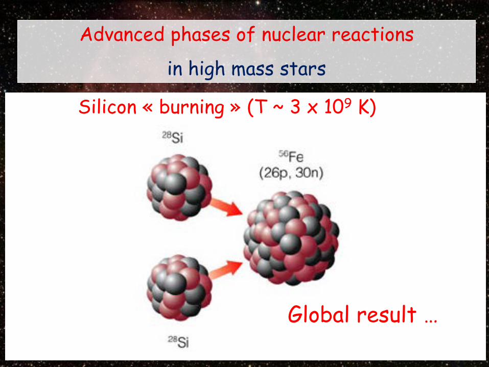
Global result …
Silicon « burning » (T ~ 3 x 10⁹ K)
Advanced phases of nuclear reactions
in high mass stars

γSHeSi +⇔+ 32
16
4
2
28
14
γ+⇔+ CaHeAr 40
20
4
2
36
18
γ+⇔+ ArHeS 36
18
4
2
32
16
• •
Complicated network !
kT <~ Q for the weakly linked nuclei ) photodisintegrations and a captures towards more stable nuclei ) rearrangement: Fe, Ni %, …
α captures:
Fe
Advanced phases of nuclear reactions
in high mass stars
Silicon « burning » (T ~ 3.3 x 10⁹ K)

Nuclear thermodynamic equilibrium (T ~ 7 x 10⁹ K) kT <~ Q for most reactions ) nuclear thermodynamic equilibrium ) Equal rates of direct and inverse reactions ) Abundance ratios given by « Saha-like » equations:
All abundances are obtained if np and nn are given ) 2 additional constraints are required : Fixed because equilibrium well before the β disintegrations
Advanced phases of nuclear reactions
in high mass stars
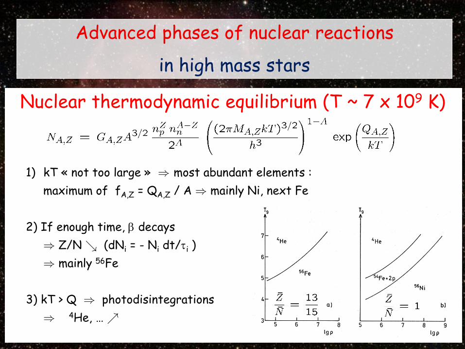
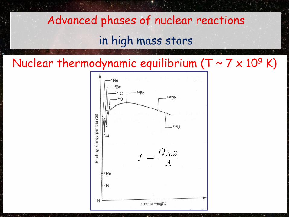
1) kT « not too large » ) most abundant elements : maximum of fA,Z = QA,Z / A ) mainly Ni, next Fe 2) If enough time, β decays ) Z/N & (dNi = - Ni dt/τi ) ) mainly 56Fe 3) kT > Q ) photodisintegrations ) 4He, … %
Advanced phases of nuclear reactions
in high mass stars
Nuclear thermodynamic equilibrium (T ~ 7 x 10⁹ K)

Core of a pre-supernova
Hydrogen Helium Carbon Oxygen Silicon Iron
Onion-like structure
Duration of ultimate phase (15 M¯) : Burning of Carbon : ~ 6000 ans Neon : ~ 7 ans Oxygen : ~ 2 ans Silicon : ~ 6 jours
Advanced phases of nuclear reactions
in high mass stars
Nuclear thermodynamic equilibrium (T ~ 7 x 10⁹ K)
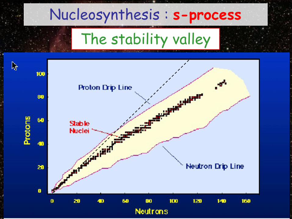
The stability valley Nucleosynthesis : s-process
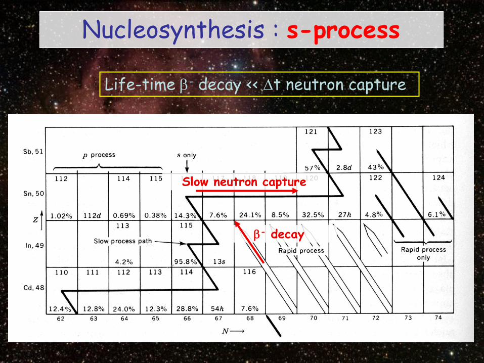
Slow neutron capture
β- decay
Nucleosynthesis : s-process
Life-time β- decay << ∆t neutron capture

Nucleosynthesis : s-process

Nucleosynthesis : s-process

Life-time β- decay >> ∆t neutron capture
1) Neutrons source: Electrons capture by the nuclei: endothermal reaction
2) Rapid neutrons capture process: Just after the nuclear reactions due to the chock wave passage, the
heavy nuclei capture very quickly the produced free neutrons:
r-process
Nucleosynthesis : r-process

Nucleosynthesis : r-process
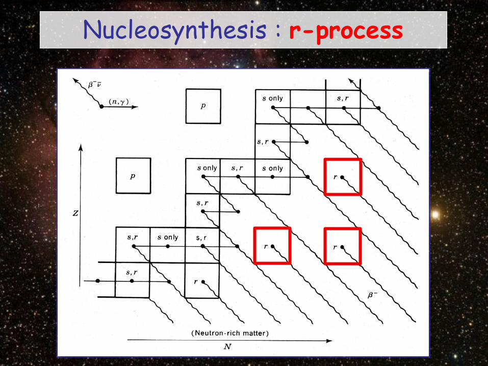
Nucleosynthesis : r-process
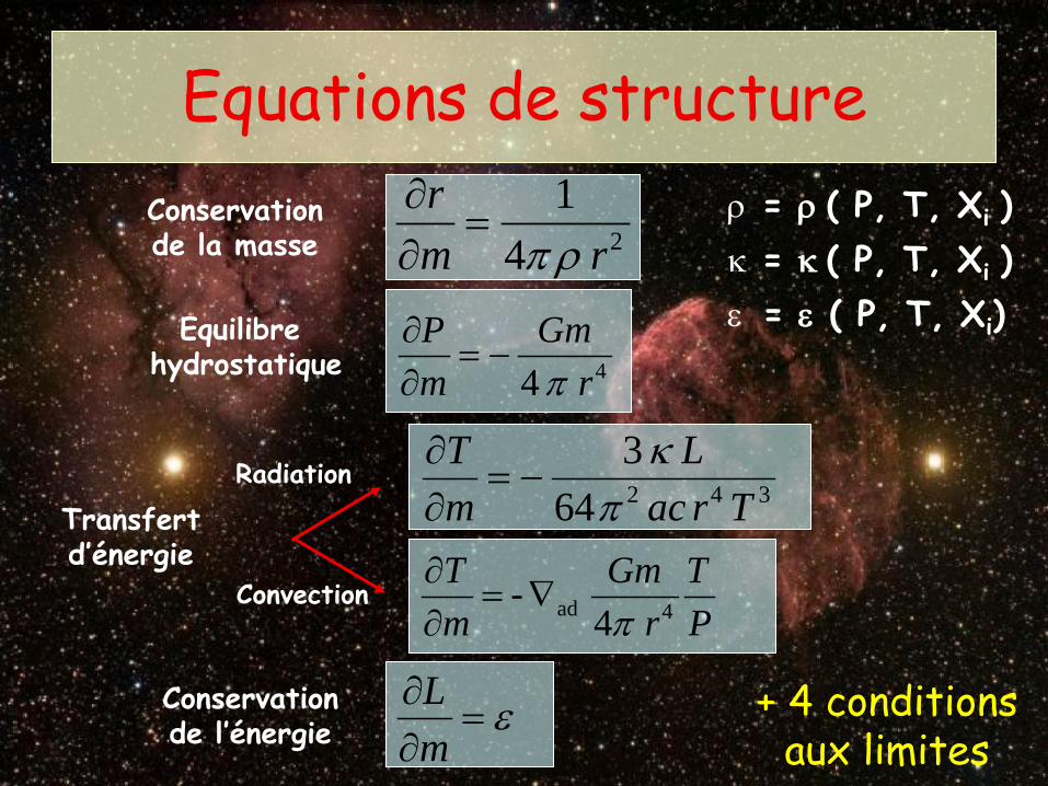
Equations de structure
241
rmr
ρπ=
∂∂Conservation
de la masse
4 4 rGm
mP
−=
∂∂
πEquilibre
hydrostatique
342643
TracL
mT
πκ
−=∂∂
Radiation
PT
rGm
mT
4ad 4 -
π∇=
∂∂
Convection
Transfert d’énergie
ε=∂∂mLConservation
de l’énergie
+ 4 conditions aux limites
ρ = ρ ( P, T, Xi ) κ = κ ( P, T, Xi ) ε = ε ( P, T, Xi)
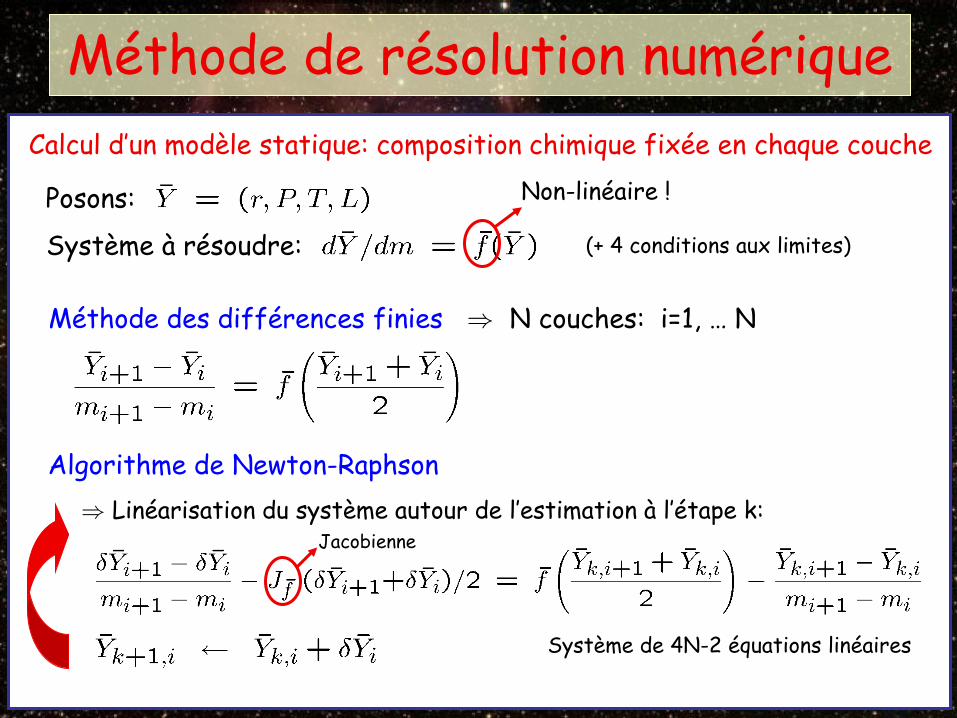
Méthode de résolution numérique
+ 4 conditions aux limites
Posons:
Système à résoudre:
Non-linéaire !
Méthode des différences finies ) N couches: i=1, … N
(+ 4 conditions aux limites)
Système de 4N-2 équations linéaires
Algorithme de Newton-Raphson ) Linéarisation du système autour de l’estimation à l’étape k:
Calcul d’un modèle statique: composition chimique fixée en chaque couche
Jacobienne

Méthode de résolution numérique
+ 4 conditions aux limites
Posons:
Système à résoudre:
Non-linéaire !
Méthode des différences finies ) N couches: i=1, … N
Algorithme de Newton-Raphson ) Linéarisation du système autour de l’estimation à l’étape k:
Calcul d’un modèle statique: composition chimique fixée en chaque couche
Jacobienne
(+ 4 conditions aux limites) CL 1 CL 2 1-2 1-2 1-2 1-2 2-3 2-3 2-3 2-3 3-4 3-4 3-4 3-4
VARIABLES Système de 4N-2 équations linéaires
E Q U A T I O N S

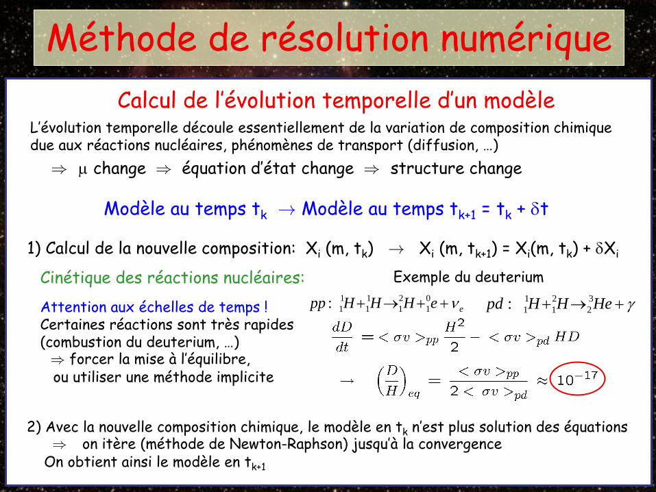
Calcul de l’évolution temporelle d’un modèle L’évolution temporelle découle essentiellement de la variation de composition chimique due aux réactions nucléaires, phénomènes de transport (diffusion, …)
Modèle au temps tk ! Modèle au temps tk+1 = tk + δt
1) Calcul de la nouvelle composition: Xi (m, tk) ! Xi (m, tk+1) = Xi(m, tk) + δXi
) µ change ) équation d’état change ) structure change
2) Avec la nouvelle composition chimique, le modèle en tk n’est plus solution des équations ) on itère (méthode de Newton-Raphson) jusqu’à la convergence On obtient ainsi le modèle en tk+1
Cinétique des réactions nucléaires: Attention aux échelles de temps ! Certaines réactions sont très rapides (combustion du deuterium, …) ) forcer la mise à l’équilibre, ou utiliser une méthode implicite
Méthode de résolution numérique
Calcul de l’évolution temporelle d’un modèle L’évolution temporelle découle essentiellement de la variation de composition chimique due aux réactions nucléaires, phénomènes de transport (diffusion, …)
Modèle au temps tk ! Modèle au temps tk+1 = tk + δt
1) Calcul de la nouvelle composition: Xi (m, tk) ! Xi (m, tk+1) = Xi(m, tk) + δXi
) µ change ) équation d’état change ) structure change
2) Avec la nouvelle composition chimique, le modèle en tk n’est plus solution des équations ) on itère (méthode de Newton-Raphson) jusqu’à la convergence On obtient ainsi le modèle en tk+1
Cinétique des réactions nucléaires: γ+→+ HeHHpd 3
221
11 :Attention aux échelles de temps !
Certaines réactions sont très rapides (combustion du deuterium, …) ) forcer la mise à l’équilibre, ou utiliser une méthode implicite
Exemple du deuterium
eeHHHpp ν++→+ 01
21
11
11 :
Méthode de résolution numérique
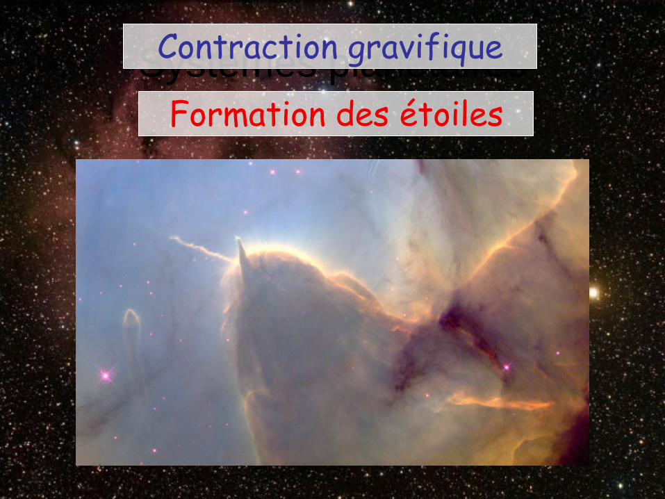
Systèmes planétaires Contraction gravifique
Formation des étoiles

Formation des étoiles
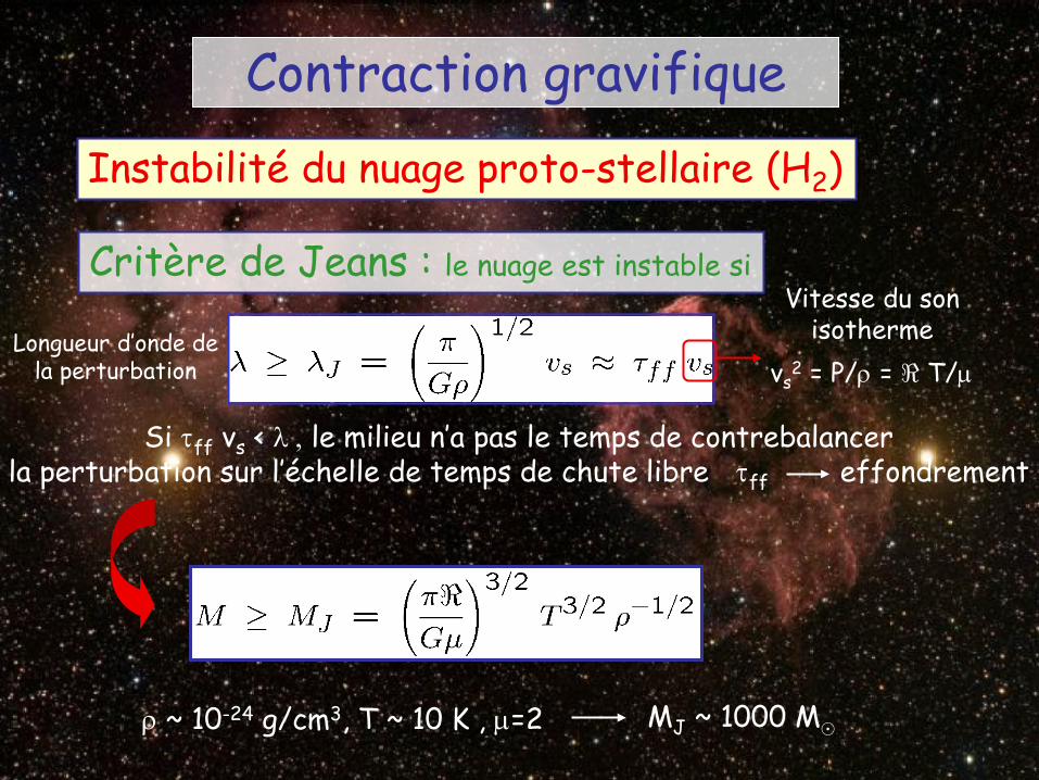
Contraction gravifique Instabilité du nuage proto-stellaire (H2)
Critère de Jeans : le nuage est instable si
ρ ~ 10-24 g/cm3, T ~ 10 K , µ=2 MJ ~ 1000 M¯
Vitesse du son isotherme
Si τff vs < λ , le milieu n’a pas le temps de contrebalancer la perturbation sur l’échelle de temps de chute libre τff effondrement
Longueur d’onde de la perturbation vs
2 = P/ρ = < T/µ

Contraction gravifique
Contraction isotherme
Etape 1 : Effondrement gravifique ~ isotherme Temps de chute libre ~ (Gρ)-1/2 ~ 108 ans >> temps d’ajustement thermique ~ λ/c (milieu optiquement mince)
Fragmentations
MJ ~ ρ-1/2

Contraction gravifique Etape 1 : Effondrement gravifique ~ isotherme
Fragmentations car MJ
Etape 2 : Effondrement gravifique ~ adiabatique Quand M ~ 1 M¯, temps de chute libre ~ temps d’ajustement thermique :
Contraction adiabatique Tc, Pc • Apparition d’un 1er front d’onde de choc
(Tc ~ 2000 K) H2 H + H
• Apparition d’un 2er front d’onde de choc
• Equilibre hydrostatique

Etape 3 : Contraction gravifique tout en maintenant l’équilibre hydrostatique
Théorème du Viriel
Energie potentielle gravifique totale
44 rmG
mP
−=
∂∂
π ρπ 241rm
r
=∂∂Equilibre
hydrostatique Masse
Gaz parfait ionisé dégénéré ou non, non-relativiste
Ei = s0M u dm Eg = - 2 Ei
Intégration par partie

Etape 3 : Contraction gravifique tout en maintenant l’équilibre hydrostatique
Théorème du Viriel
(Gaz parfait) Eg = - 2 Ei
Temps d’Helmoltz – Kelvin : τHK = GM2 / (2 R L)
Etot = Ei + Eg Energie totale :
Conservation de l’énergie globale sans production interne
Pas de réactions nucléaires !
L = - dEtot /dt = – d Ei / dt – dEg / dt = dEi /dt = -(1/2) dEg / dt
L - s ε dm
Si réactions nucléaires, remplacer L par
La moitié de l’énergie potentielle gravifique libérée lors de la contraction de l’étoile conduit à une augmentation de son énergie interne, l’autre moitié est rayonnée.

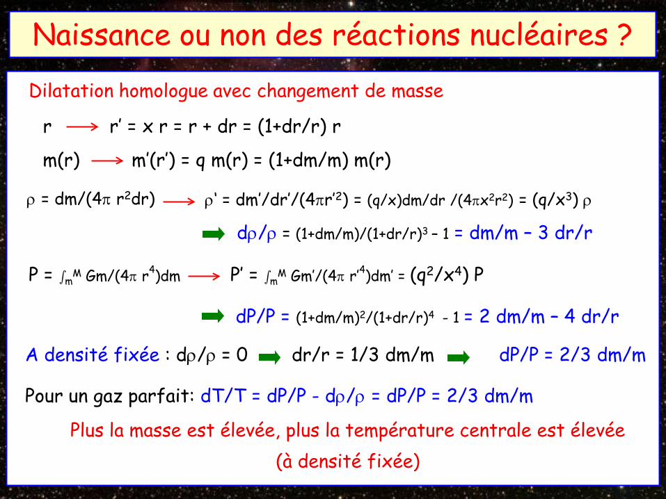
Naissance ou non des réactions nucléaires ?
Rôle de la dégénérescence
Question : lors de la contraction gravifique, Tc augmente-t-elle toujours ?
Theorème du Viriel ) P/ρ augmente Pour un gaz parfait : P/ρ / T oui pour un gaz parfait non-dégénéré
Mais … ce n’est plus le cas pour un gaz dégénéré.
r r’ = x r = r + dr = (1+dr/r) r
ρ ρ’ = ρ/x3
P=Poids P’ = Poids’ = P/x4
dρ/ρ = ρ’(m)/ρ(m) – 1 = 1/(1+dr/r)3 - 1 = – 3 dr/r
dP/P = P’(m)/P(m) – 1 = 1/(1+dr/r)4 - 1 = – 4 dr/r
Contraction homologue
dr/r = x-1 = cst

Rôle de la dégénérescence
Equation d’état générale : dρ/ρ = α dP/P - δ dT/T
dT/T = (α/δ) dP/P - (1/δ) dρ/ρ = (4α-3)/(3δ) dρ/ρ
dP/P = (4/3) dρ/ρ
Naissance ou non des réactions nucléaires ?
r r’ = x r = r + dr = (1+dr/r) r
ρ ρ’ = ρ/x3
P P’ = P/x4
dρ/ρ = ρ’(m)/ρ(m) – 1 = 1/(1+dr/r)3 - 1 = – 3 dr/r
dP/P = P’(m)/P(m) – 1 = 1/(1+dr/r)4 - 1 = – 4 dr/r
Contraction homologue
dr/r = x-1 = cst

Rôle de la dégénérescence
dT/T = (4α-3)/(3δ) dρ/ρ
Pour un gaz parfait : α = 1 , δ = 1 dT/T = (1/3) dρ/ρ non-dégénéré
Naissance ou non des réactions nucléaires ?
Pour un gaz dégénéré : α = 3/5 , δ = 0 dT/T = - 1 dρ/ρ non-relativiste
dρ/ρ = α dP/P - δ dT/T
T
T
L’énergie gravifique libérée lors de la contraction n’est pas suffisante pour accélérer les électrons dégénérés (énergie de Fermi ). L’énergie manquante est puisée dans l’énergie cinétique des ions non- dégénérés de sorte que la température diminue.

Pour un gaz dégénéré : dT/T = - ∞ dρ/ρ non-relativiste
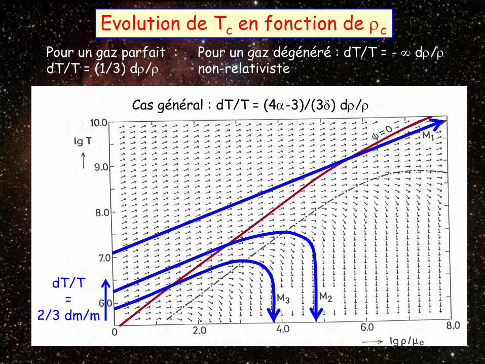
ψ : paramètre de dégénérescence
Pour un gaz parfait : dT/T = (1/3) dρ/ρ
Cas général : dT/T = (4α-3)/(3δ) dρ/ρ
Pente 1/3
Pente 2/3 ρT-3/2 = cte
Cas général : dT/T = (4α-3)/(3δ) dρ/ρ
Naissance ou non des réactions nucléaires ?
r r’ = x r = r + dr = (1+dr/r) r
Dilatation homologue avec changement de masse
A densité fixée : dρ/ρ = 0 dr/r = 1/3 dm/m dP/P = 2/3 dm/m
Pour un gaz parfait: dT/T = dP/P - dρ/ρ = dP/P = 2/3 dm/m
Plus la masse est élevée, plus la température centrale est élevée (à densité fixée)
ρ = dm/(4π r2dr)
dP/P = (1+dm/m)2/(1+dr/r)4 - 1 = 2 dm/m – 4 dr/r
P = smM Gm/(4π r4)dm
m(r) m’(r’) = q m(r) = (1+dm/m) m(r)
ρ‘ = dm’/dr’/(4πr’2) = (q/x)dm/dr /(4πx2r2) = (q/x3) ρ
dρ/ρ = (1+dm/m)/(1+dr/r)3 – 1 = dm/m – 3 dr/r
P’ = smM Gm’/(4π r’4)dm’ = (q2/x4) P
Pour un gaz parfait : dT/T = (1/3) dρ/ρ
Pour un gaz dégénéré : dT/T = - ∞ dρ/ρ non-relativiste
Cas général : dT/T = (4α-3)/(3δ) dρ/ρ
Evolution de Tc en fonction de ρc
dT/T =
2/3 dm/m
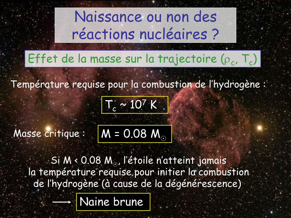
Effet de la masse sur la trajectoire (ρc, Tc)
Naissance ou non des réactions nucléaires ?
Température requise pour la combustion de l’hydrogène :
Tc ~ 107 K
Masse critique : M = 0.08 M¯
Si M < 0.08 M¯, l’étoile n’atteint jamais la température requise pour initier la combustion de l’hydrogène (à cause de la dégénérescence)
Naine brune

Energie potentielle gravifique totale
Ei, tot = s0M u dm = 3/2 s0
Μ (P/ρ) dm
Eg = - 2 Ei, tot
-1/2 dEg/dt = L = dEi /dt
Refroidissement des naines brunes et blanches
Energie interne totale
Théorème du Viriel
L’énergie interne totale augmente lors de la contraction d’un gaz dégénéré (naine blanche) aussi !!

-1/2 δ Eg = δ Ei,tot
Les naines blanche : refroidissement
Ei, tot : Energie interne totale (ions + électrons)
Eg : Energie potentielle gravifique
Théorème du Viriel
Ee : Energie interne des électrons
Eions << Ee
Toute l’énergie gravifique libérée augmente l’énergie cinétique des électrons
δρ/ρ = cst.
= - 3 δr/r
Eg = - 2 Ei, tot

Les naines blanches : refroidissement
Toute l’énergie gravifique libérée augmente l’énergie cinétique des électrons
L = - dEtot /dt = - d Eions /dt – d Ee /dt – d Eg /dt = - d Eions /dt
Toute l’énergie rayonnée est puisée dans l’énergie cinétique des ions
Découplage
Hydrostatique, gravité : Gaz d’électrons
Thermique : Gaz d’ions
La température diminue

Les naines blanches : refroidissement
L = - d Eions /dt = - cv M dT0 /dt
Toute l’énergie rayonnée est puisée dans l’énergie cinétique des ions
Eions = s0M uions dm = cv T0 M
Cœur quasi isotherme (conduction électronique très efficace)
La température diminue lentement

Panorama des scénarios possibles d’évolution des étoiles
Naine brune
Combustion de l’Hydrogène
M < 0.08 M¯
T ' 107 K
Tem
péra
ture
cen
trale
temps
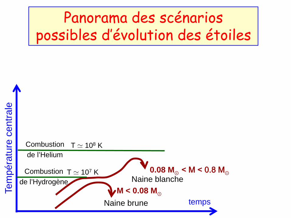
Panorama des scénarios possibles d’évolution des étoiles
Naine brune
Naine blanche Combustion
de l’Hydrogène
Combustion de l’Helium
0.08 M¯ < M < 0.8 M¯
M < 0.08 M¯
T ' 107 K
T ' 108 K
Tem
péra
ture
cen
trale
temps

Panorama des scénarios possibles d’évolution des étoiles
Naine brune
Naine blanche Combustion
de l’Hydrogène
Combustion de l’Helium
Combustion du Carbone
Naine blanche 0.8 M¯ < M < 9 M¯
0.08 M¯ < M < 0.8 M¯
M < 0.08 M¯
T ' 108 K
T ' 107 K
T ' 6 £ 108 K
Tem
péra
ture
cen
trale
temps
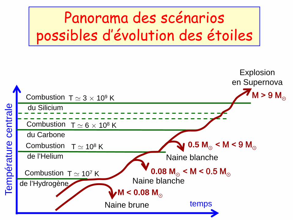
Panorama des scénarios possibles d’évolution des étoiles
Tem
péra
ture
cen
trale
Naine brune
Naine blanche Combustion
de l’Hydrogène
Combustion de l’Helium
Combustion du Carbone
Combustion du Silicium
Naine blanche
Explosion en Supernova
M > 9 M¯
0.5 M¯ < M < 9 M¯
0.08 M¯ < M < 0.5 M¯
M < 0.08 M¯
T ' 108 K
T ' 107 K
T ' 6 £ 108 K
T ' 3 £ 109 K
temps

Panorama des scénarios possibles d’évolution des étoiles