Diane Redekop FINALTHESISS

The Examination of Hemispherical Photography as a means of obtaining In Situ Remotely Sensed Sky Gap Estimates in Snow-Covered Coniferous Environments

by

Diane Evelyne Redekop

A thesis presented to the University of Waterloo

in fulfillment of the thesis requirement for the degree of Master of Environmental Studies

in Geography

Waterloo, Ontario, Canada, 2008

© Diane Evelyne Redekop 2008

ii

AUTHOR’S DECLARATION

I hereby declare that I am the sole author of this thesis. This is a true copy of the thesis,

including any required final revisions, as accepted by my examiners.

I understand that my thesis may be made electronically available to the public.

iii

ABSTRACT

In remote sensing, the application determines the type of platform and scale used during

air or space –borne data collection as the pixel size of the collected data varies depending on the

sensor or platform used. Applications involving some cryospheric environments require the use

of the microwave band of the electromagnetic spectrum, with snow water equivalent (SWE)

studies making use of passively emitted microwave radiation.

A key issue in the use of passive microwave remotely sensed data is its spatial resolution,

which ranges from 10 to 25 kilometres. The Climate Research Branch division of the

Meteorological Service Canada is using passive microwave remote sensing as a means to

monitor and obtain SWE values for Canada’s varying land-cover regions for use in climate

change studies. Canada’s diverse landscape necessitated the creation of a snow water equivalent

retrieval algorithm suite comprised of four different algorithms; all reflecting different vegetative

covers. The spatial resolution of small scale remotely sensed data does provide a means for

monitoring Canada’s large landmass, but it does, however, result in generalizations of land-

cover, and in particular, vegetative structure, which is shown to influence both snow cover and

algorithm performance.

The Climate Research Branch is currently developing its SWE algorithm for Canada’s

boreal forest region. This thesis presents a means of successfully and easily collecting in situ

remotely sensed data in the form of hemispherical photographs for gathering vegetative structure

data to ground-truth remotely sensed data. This thesis also demonstrates that the Gap Light

Analyzer software suite used for analyzing hemispherical photographs of mainly deciduous

environments during the spring-fall months can be successfully applied towards cryospheric

studies of predominantly coniferous environments.

iv

ACKNOWLEDGEMENTS

Dr. LeDrew I would like to thank Dr. Ellsworth LeDrew for his guidance, limitless opportunities, never-ending ear, and for most of all, his patience.

Jefferson You have brought focus and calmness to my life, which has allowed me to see the difference between things I need and those I want.

Mensa Thank you to my cat, Mensa, for doing what he does best: listening. I hope you never learn to talk for I will truly be in trouble.

Grandparents I wish you could have been here to experience the present and future with me.

Friends Thank you to my many friends for believing in their ever so frequently absent friend.

“We are the music makers, and we are the dreamers of dreams” - Willy Wonky - Arthur O'Shaughnessy

v

TABLE OF CONTENTS LIST OF TABLES......................................................................................................................................................vi

LIST OF ILLUSTRATIONS................................................................................................................................... vii

CHAPTER ONE: INTRODUCTION.......................................................................................................................1 1.1 MONITORING CRYOSPHERIC ENVIRONMENTS .....................................................................................................1 1.2 OVERVIEW OF RESEARCH PROBLEM ...................................................................................................................2 1.3 RESEARCH OBJECTIVES ......................................................................................................................................4 1.4 THESIS ORGANIZATION.......................................................................................................................................5

CHAPTER TWO: LITERATURE REVIEW..........................................................................................................7 2.1 BASIC PRINCIPLES OF PASSIVE MICROWAVE REMOTE SENSING OF SWE ...........................................................7 2.2 FACTORS THAT INFLUENCE PASSIVE MICROWAVE EMISSIONS/SWE ESTIMATES ................................................8 2.3 CURRENT STATE OF RESEARCH FOR PASSIVE MICROWAVE REMOTE SENSING OF PRAIRIE SWE .....................14 2.4 CURRENT STATE OF RESEARCH FOR IN-SITU REMOTE SENSING OF FOREST ENVIRONMENTS ............................18 2.5 CURRENT STATE OF RESEARCH FOR ANALYZING HEMISPHERICAL PHOTOGRAPHS ..........................................28

CHAPTER THREE: METHODOLOGY ..............................................................................................................32 3.1 INTRODUCTION .................................................................................................................................................32 3.2 PRELIMINARY STUDY: BOREAL FOREST SNOW WATER EQUIVALENT SCALING EXPERIMENT ..........................33 3.3 SECONDARY STUDY: FEBRUARY 2004 MSC EXPERIMENT ...............................................................................36 3.4 THESIS STUDY: FEBRUARY 2004 HEMISPHERICAL PHOTOGRAPHY EXPERIMENT..............................................36 3.5 SENSOR PLATFORM PREPARATION....................................................................................................................42 3.6 ANALYSIS .........................................................................................................................................................49

CHAPTER FOUR: DATA ANALYSIS AND RESULTS .....................................................................................51 4.1 DATA ANALYSIS DESIGN ..................................................................................................................................51 4.2 ANALYSIS OF VARIANCE...................................................................................................................................52 4.3 OUTPUT TABLE .................................................................................................................................................53 4.4 NULL HYPOTHESES ...........................................................................................................................................55 4.5 EXPERIMENTAL ERROR .....................................................................................................................................56 4.6 CONCLUSION FOR EXPERIMENTAL ERROR ........................................................................................................61 4.7 PROCESSING ERROR..........................................................................................................................................61 4.8 CONCLUSION FOR PROCESSING ERROR .............................................................................................................65 4.9 CONCLUSION.....................................................................................................................................................65

CHAPTER FIVE: SUMMARY AND CONCLUSIONS.......................................................................................66 5.1 INTRODUCTION .................................................................................................................................................66 5.2 MAJOR FINDINGS ..............................................................................................................................................69 5.3 SOURCES OF ERROR ..........................................................................................................................................72 5.4 FUTURE RESEARCH DEMANDS..........................................................................................................................73

APPENDICES

APPENDIX 1.0 ..........................................................................................................................................................74 1.1 GLA© OUTPUT DATA FOR POPULATIONS 1 THROUGH 3....................................................................................74

APPENDIX 2.0 ..........................................................................................................................................................76 2.1 ACRONYM LIST .........................................................................................................................................76 2.2 SOFTWARE LIST ........................................................................................................................................76

REFERENCES ..........................................................................................................................................................77 ACADEMIC REFERENCES .................................................................................................................................77 INTERNET REFERENCES ...................................................................................................................................81

vi

LIST OF TABLES

Table 2.1: Snow cover Parameters and their Influence on SWE Algorithm Performance............ 9 Table 2.2: Strategies for Compensating for Issues of Scale in Forest Stand Research ............... 11 Table 2.3: Radial Projection Characteristics................................................................................ 22 Table 3.1: Description of Data Populations................................................................................. 46 Table 4.1: ANOVA Output Table................................................................................................ 54 Table 4.2: Variables used during Experimental Error Analysis .................................................. 56 Table 4.3: ANOVA Summary – Dataset 1 to Dataset 2 (Observations 0º to 5º)......................... 57 Table 4.4: ANOVA Summary – Dataset 1 to Dataset 3 (Observations 0º to 10º)....................... 59 Table 4.5: ANOVA Summary – Dataset 2 to Dataset 3 (Observations 5 º to 10 º)..................... 59 Table 4.6: ANOVA Summary – Dataset 1 to Dataset 4 (Observations 0 º to 20 º)..................... 60 Table 4.7: Variables used during Processing Error Analysis ...................................................... 62 Table 4.8: ANOVA Summary – 0° Observations only (Dataset 5 to Dataset 6)......................... 63 Table 4.9: ANOVA Summary – 0° Observations only (Dataset 5 to Dataset 7)......................... 64 Table 4.10: ANOVA Summary – 0° Observation 1 .................................................................... 64 Table 5.1: Current Organizations monitoring and providing information about Canada’s Cryosphere .................................................................................................................................... 67

vii

LIST OF ILLUSTRATIONS

Figure 2.1: Cryosphere-Climate Interactions................................................................................. 8 Figure 2.2: Main Co-ordinators of SWE Algorithm Suite........................................................... 16 Figure 3.1: BERMS Study Area used for Winter 2003 Scaling Experiment............................... 33 Figure 3.2: Sample Problematic Hemispherical Photograph from Winter 2003 Experiment ..... 35 Figure 3.3: Procedures in a Digital Photography Derived Sky Gap Estimates Task................... 37 Figure 3.4: Map and Airphoto of Macton Agreement Forest ...................................................... 39 Figure 3.5: Macton Agreement Forest ......................................................................................... 40 Figure 3.6: Macton Agreement Forest – Sample Vegetative Structure ....................................... 41 Figure 3.7: Macton Agreement Forest – Sample Management History ...................................... 41 Figure 3.8: Hemispherical Photograph Experiment Design ........................................................ 43 Figure 3.9: Controlled Experimental Error (Population 1).......................................................... 45 Figure 3.10: Population 2 Sample Dataset................................................................................... 47 Figure 3.11: Population 3 Threshold Modification...................................................................... 48

1

CHAPTER ONE: Introduction

1.1 Monitoring Cryospheric Environments In 2001, Canada experienced a national drought, with the situation compounded in the

Prairie region during a warmer and drier than normal 2001-2002 winter. Low snow

accumulation in the Prairies meant minimal runoff during the spring of 2002, which left that

region with water shortages, in addition to low soil moisture levels. Impacts from low snow

accumulation in Canada’s Prairie region include lower annual crop yields and unreliable and

uncertain industry (Agriculture and Agri-Food Canada [agr.gc.ca/pfra/drought02sum_e.htm]

October, 2006).

The Prairie region drought of 2001-2002 highlights how Canada is increasingly

experiencing negative impact associated with changes in its climate, especially in its cryospheric

environments. The cryosphere refers to frozen natural phenomena within the world’s climate

system. These phenomena include river, sea and lake ice, seasonal snow cover, glaciers, and

permafrost (SOCC [socc.ca], October 2006; LeDrew, 2002). Large cryosphere environments are

degrading from climate change and industrialization, resulting in ecosystem diversity being

threatened, physical features being altered, and industry being on alert. Canada is at the forefront

of this issue because of its variety of cryospheric environments, significant Arctic region, and

resource-based economy (LeDrew et al., 1995). Seasonal snow cover is one component of the

cryosphere that is impacted by climate change, and Canada’s increasingly variable snow

accumulation is resulting in negative conditions similar to those experienced during the 2001-

2002 Prairie region drought.

Canada has six main snow cover regions: tundra, taiga (boreal forest), Prairie, maritime,

alpine and ephemeral. These regions are based on climate and snow characteristics, including:

snow extent; depth; water equivalent; structure; wetness; and surface albedo/reflectivity (Barry et

2

al., 1993; Barry et al., 1994; Goodison, 1995; Sturm et al., 1995 in Ross, 1996).

Snow cover, a component of the cryosphere, has a snow water equivalent (SWE1)

characteristic that is determined from snow depth and density and represents the depth of water

that would result if snow were melted (SOCC [socc.ca], October 2006). SWE is currently being

used by the Meteorological Service of Canada’s Climate Research Branch to identify snow

accumulation and depth. Derksen et al. (2002, pg. 203) describe SWE as an important

component of climate models because of the,

“climatological impacts of snow distribution on local, regional, and hemispheric energy exchange and the hydrological significant of snowpack water storage.”

SWE provides crucial information concerning water available for irrigation, hydroelectric power

generation, industry and human consumption (Barry et al., 1993; Derksen, 2001; LeDrew, 2002).

SWE has played an important role in Canadian water issues; most recently, it was used in

2002 to identify low snow accumulation in the Prairies, which subsequently resulted in crop

failure brought on by insufficient soil moisture levels (LeDrew, 2002). That project highlights

the utility of SWE in forecasting and modeling Canadian cryosphere and water issues. This

example utilized a prairie SWE retrieval algorithm, developed by Environment Canada’s

Meteorological Service of Canada (MSC), and made use of data collected by satellite remote

sensing2 to obtain SWE surface measurements.

1.2 Overview of Research Problem Remote sensing, a method of collecting information about the earth’s surface without

physical contact, is a valuable tool for obtaining snow cover data. This technology has the

capability to provide “quantitative, repetitive and spatially continuous observations” over large

1 All acronyms are summarized at the end of the thesis in Appendix 2.1. 2 In this thesis, ‘satellite remote sensing’ refers to space-based platforms.

3

areas (Derksen et al., 2002a, pg. 1). Obtaining comparable snow cover data, like SWE

measurements, through terrestrial sampling is difficult. Extreme climate and terrain conditions

can make it near impossible.

The MSC has developed a suite of operational, passive microwave SWE retrieval

algorithms that makes use of data derived from both terrestrial and remotely sensed sources

(using airborne and satellite acquisition programs) for the different snow cover and terrestrial

regions of central Canada, beginning in the 1980s with the development of a SWE algorithm for

Canada’s prairie region (see Goodison et al., 1995; Goita et al., 1997 in Derksen et al., 2002;

Derksen et al., 2002a). Derksen (2001; 2002) applied the prairie SWE algorithm to other

Canadian snow cover regions, but determined that standing vegetation structure, characteristics

of the remotely sensed data including pixel size, and variable physical properties of the snow

cover negatively impact the accuracy of the prairie SWE algorithm in non-prairie environments.

Standing vegetation structure, for instance, results in the absorption, emission and scattering of

microwave energy, and interception of falling snow (Foster et al., 1991 in Derksen et al., 2000).

Remotely sensed passive microwave data has a spatial resolution that ranges from 10 to

25 kilometres. Obtaining SWE derived measurements using passive microwave data with a

spatial resolution of 25 kilometres will retrieve only one SWE value for 625 kilometres2. This

consequently assumes spatial homogeneity with regards to the local land-cover and snow cover.

Land-cover and snow cover, particularly in regions outside of the prairies are, however,

heterogeneous, and are difficult to accurately account for with the small scale of passive

microwave derived data because all features in a pixel area are generalized to obtain one pixel

value. Derksen (2001; 2002) concluded that the influence of these outside factors do not allow

the prairie SWE algorithm to be effectively implemented in non-prairie environments.

4

Consequently, research at the MSC has since focused on land-cover specific SWE retrieval

algorithms, including one for the boreal snow cover region of central Canada, to augment the

algorithm suite (Derksen et al., 2002a).

The MSC is focusing on developing the boreal SWE algorithm, and Canada’s

heterogeneous landscape and snow cover requires collecting several types of auxiliary data,

including in situ snow cover data (depth, density, SWE) and second order land-cover variables

(vegetative structure characteristics and canopy closure, etc.) (IGBP, 1992; and Houghton et al.,

1996 in Curran et al., 1998; Derksen, 2002). Hemispherical photography is considered a suitable

ground-based (in situ) remote sensing tool for indirectly measuring forest canopy architecture

and light interception (Fournier et al., 1996; 1997; 2003).

Hemispherical photography assesses variation in vegetation on a large scale, making this

tool sensitive to local scale variations in forest canopy structure. The collection of hemispherical

photography makes use of a sensor (the camera with a hemispherical lens) facing skyward from

beneath the forest canopy to measure light transmission and forest canopy structure (Fournier et

al., 2003; Frazer et al., 1999). The open area, or gaps, within the forest canopy is referred to as

sky gap, and sky gap values can help describe the density of the neighbouring forest canopy.

1.3 Research Objectives

The objective of this thesis is to examine and test the use of hemispherical photography

as a means of obtaining in situ remotely sensed sky gap estimates in snow-covered

predominantly coniferous environments. Two field programs were designed around the

collection of in situ, airborne and remotely sensed snow water equivalent measurements, which

also incorporated the collection of hemispherical photography of the vegetative canopy to attain

this objective. By varying the conditions by which the hemispherical photographs of the forest

5

canopy were taken, including angle from horizontal, cloud cover, and height above the ground,

in this thesis we will determine if hemispherical photography can easily and successfully be used

as a means for obtaining in situ sky gap values for snow-covered predominantly coniferous

environments.

The motivation behind this research is to find a correction factor for the passive

microwave sensor in order to be able to interpret and better understand all surface land-cover

types and obtain more representative remotely sensed SWE values (Derksen et al., 2000). Once

the utility of hemispherical photography and its use as a correction factor is determined and

understood, this information can be applied to MSC’s remaining SWE passive microwave

algorithms by incorporating forest canopy research structure in studies concerning cryospheric

environments.

1.4 Thesis Organization Themes covered in the first chapter included cryospheric environments; SWE algorithm

suite development; land-cover variability; in situ and satellite remote sensing; hemispherical

photography; sky gap; measurement sensitivity and the application of in situ land-cover

measurement to remotely sensed SWE data.

In chapter two, a brief overview of the historical context of this thesis’ research

application is provided. This includes a description of SWE algorithm suite development, how

both snow and vegetative structure impact remotely sensed data and its collection, and to a

discussion concerning the current state of research and application for in situ remote sensing of

forested environments. An introduction to two different software suites that analyze

hemispherical photography is also provided.

6

In chapter three, the methodology, various study sites and collection of hemispherical

photography are described. Data analysis and results are described in chapter four, with chapter

five containing major findings, conclusions and suggestions for research. Suggestions for future

research focus on extending the thesis findings, exploring hemispherical photography

applications in coniferous environments and cryospheric environments, and improving the

accuracy of the SWE algorithm suite.

7

CHAPTER TWO: Literature Review

2.1 Basic Principles of Passive Microwave Remote Sensing of SWE Remote sensing involves acquiring imagery or data with varying spatial and radiometric

resolutions about the earth’s surface from airborne or satellite platforms (Richards and Jia,

1999). Remotely sensed digital images contain data in the form of two-dimensional pixels that

reflect the spatial resolution of the sensor, and this data has varying brightness values based on

its radiometric resolution (Avery and Berlin, 1985). The microwave band of the electromagnetic

spectrum has a wavelength between 0.1 and 30 centimetres. There are two methods of remotely

sensing microwave radiation; passive or active. Passive remote sensing involves detecting

microwave radiation that is naturally emitted from the earth’s surface, whereas active remote

sensing utilizes energy transmitted from the remote sensing platform itself (Richards and Jia,

1999; Avery and Berlin, 1985). Small scale remotely sensed imagery has the benefit of covering

a large area, but in the case of a passive microwave pixel its spatial resolution, ranging from 10

to 25 kilometres, can negatively influence the accuracy of intra-pixel variability of land cover

characteristics, including vegetation structure (Derksen, 2002). Large spatial resolutions such as

those experienced in passive microwave derived-SWE data result in questions of scale and

variability, which will be addressed later in the chapter. In the context of this thesis, small scale

remotely sensed data refers to passive microwave data, whereas in situ hemispherical

photography refers to large scale data.

The use of satellite and airborne remote sensing can be an effective tool for use in land

cover monitoring for scientific studies, resource management and human activities; such as

monitoring the clean-up of the 9/11 terrorist attacks on New York’s World Trade Center twin-

towers (Cihlar, 2000, National Park Service [home.nps.gov/gis/applications/wtcgis.html] April,

2008).

8

2.2 Factors that influence Passive Microwave emissions/SWE estimates Canada’s research and development into SWE monitoring is out of necessity as the

country hosts a variety of cryospheric components over large geographical areas, including snow

and ice. In a show of national and global responsibility towards cryospheric research, the

Canadian government is an invested stakeholder into furthering the measuring, modeling, and

understanding of relationships between the cryosphere surface and atmosphere energy exchanges

(Piwowar et al., 2002; Brown, 1996; Barry et al., 1994). Research examining changes in snow

cover has identified that these alterations, such as the breaking-up of glaciers, can be

compounded by changes in atmospheric conditions, including air temperature and radiation

(World Glacier Monitoring Service [geo.unizh.ch/wgms/monitoring.html] April, 2008). As a

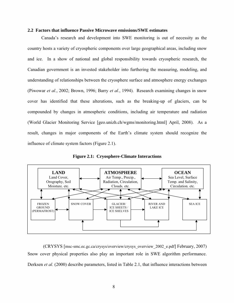
result, changes in major components of the Earth’s climate system should recognize the

influence of climate system factors (Figure 2.1).

Figure 2.1: Cryosphere-Climate Interactions

(CRYSYS [msc-smc.ec.gc.ca/crysys/overview/crysys_overview_2002_e.pdf] February, 2007)

Snow cover physical properties also play an important role in SWE algorithm performance.

Derksen et al. (2000) describe parameters, listed in Table 2.1, that influence interactions between

LAND Land Cover,

Orography, Soil Moisture, etc.

ATMOSPHERE Air Temp., Precip.,

Radiation, Circulation, Clouds, etc.

OCEAN Sea Level, Surface Temp. and Salinity,

Circulation, etc.

FROZEN GROUND

(PERMAFROST)

SNOW COVER

GLACIER/ ICE SHEETS / ICE SHELVES

RIVER AND LAKE ICE

SEA ICE

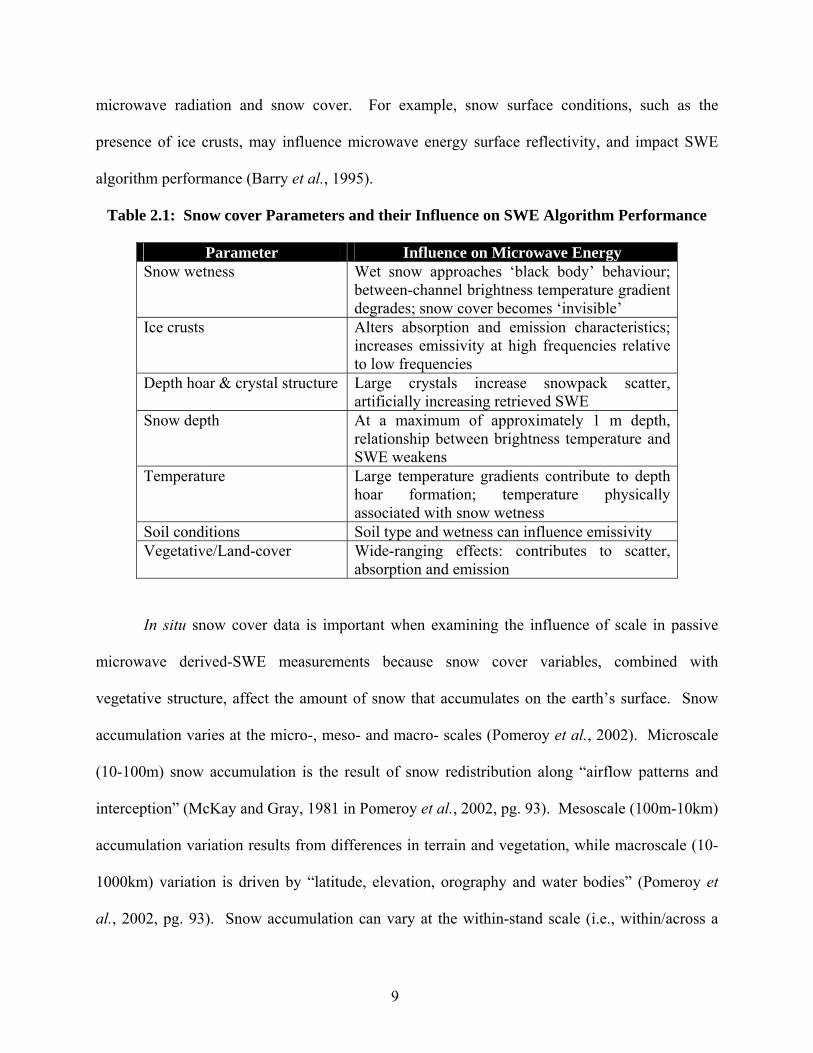
9

microwave radiation and snow cover. For example, snow surface conditions, such as the

presence of ice crusts, may influence microwave energy surface reflectivity, and impact SWE

algorithm performance (Barry et al., 1995).

Table 2.1: Snow cover Parameters and their Influence on SWE Algorithm Performance

Parameter Influence on Microwave Energy Snow wetness Wet snow approaches ‘black body’ behaviour;

between-channel brightness temperature gradient degrades; snow cover becomes ‘invisible’

Ice crusts Alters absorption and emission characteristics; increases emissivity at high frequencies relative to low frequencies

Depth hoar & crystal structure Large crystals increase snowpack scatter, artificially increasing retrieved SWE

Snow depth At a maximum of approximately 1 m depth, relationship between brightness temperature and SWE weakens

Temperature Large temperature gradients contribute to depth hoar formation; temperature physically associated with snow wetness

Soil conditions Soil type and wetness can influence emissivity Vegetative/Land-cover Wide-ranging effects: contributes to scatter,

absorption and emission

In situ snow cover data is important when examining the influence of scale in passive

microwave derived-SWE measurements because snow cover variables, combined with

vegetative structure, affect the amount of snow that accumulates on the earth’s surface. Snow

accumulation varies at the micro-, meso- and macro- scales (Pomeroy et al., 2002). Microscale

(10-100m) snow accumulation is the result of snow redistribution along “airflow patterns and

interception” (McKay and Gray, 1981 in Pomeroy et al., 2002, pg. 93). Mesoscale (100m-10km)

accumulation variation results from differences in terrain and vegetation, while macroscale (10-

1000km) variation is driven by “latitude, elevation, orography and water bodies” (Pomeroy et

al., 2002, pg. 93). Snow accumulation can vary at the within-stand scale (i.e., within/across a

10

specific stand of trees) because of the stand’s characteristics: disturbed, which is the case in a

commercial forestry zone, or in its natural state, such as in protected wilderness areas (Pomeroy

et al., 2002). Snow accumulation is typically greater in forest clearings, but the difference in

snow accumulation between disturbed and natural forests is related to the size of the clearing

(Golding et al., 1978 in Pomeroy et al., 2002). Smaller clearings tend to have accumulations

affected by, for example, neighbouring forest canopy, whereas larger clearings can lose

accumulation via wind transport (i.e., blowing snow). Variations in snow accumulation in

Saskatchewan’s boreal forest region are influenced by many factors that help prevent snow loss,

and maintain snow accumulation brought by winter snow (Pomeroy et al., 1997 in Pomeroy et

al., 2002). The factors include conditions characterized by a relatively low wind speed in the

winter, and treefellings and trimmings left at the site of a clear-cut. The treefellings and

trimmings act as natural snow fences and wind-breakers, while the low wind speed helps to

prevent snow from being blown away.

Vegetative cover in the boreal forest contains both deciduous and coniferous trees, and

although this thesis examines the sky gap of a predominantly coniferous forest stand, deciduous

canopy cover is also examined as there were deciduous trees present in the study site. Forest

canopy is defined by Howard (1991, pg. 303) as, “the proportion per unit area of the ground

covered by the vertical projection on to it of the overall tree crowns”. In this thesis we examine

forest canopy vegetative structure for obtaining sky gap measurements using in situ remote

sensing. Sky gap (also known as gap fraction) is defined by Inoue et al. (2004a, pg. 92) as, “the

total amount of sky visible as a proportion of the whole hemisphere when viewed from a point”.

Vegetative structure and sky gap are of concern in SWE studies as they can both impact

snow cover characteristics and cause variations in forest canopy light conditions. Vegetative

11

structure is of particular concern to studies using passive microwave data as the sensor’s spatial

resolution cannot take into account local changes in vegetative structure.

A strategy derived from Fournier et al. (2003) to compensate for issues of scale with

standing forest data is used to obtain data from each of the three scale levels: ground plot, stand

and regional/national (Table 2.2). Questions of scale are frequently the basis of research

problems in remote sensing and data analysis, and information about a forest canopy, such as

that found in Canada’s boreal region, should be collected at the scale required to answer the

problem (Fournier et al., 1997).

Table 2.2: Strategies for Compensating for Issues of Scale in Forest Stand Research

Spatial Scale of Interpretation

Parameter Measured Methodology

Regional Climate, ecosystem, landscape parameters

Climate statistics; maps (topography, soil, etc.); interpretation of aerial photographs

Stand Hemispherical views of canopy architecture

Catalog of hemispherical photographs

Stand Tree location; understory mapping Site characterization Individual crown Height of tree, live crown, trunk

diameter at breast height; crown horizontal extent

Site characterization

Trunk and branch units

Trunk inventory; branch segments geometry and position; branch segments topology

Vectorization

Foliage Geometric description of foliage Vectorization

(Fourniet et al., 1997)

Forest stand canopies create two major concerns for geographers: the canopy modifies incoming

solar radiation and reflects radiation, as well as creating a microclimate that impacts the

exchange of heat, water and carbon during ecophysical processes (Fournier et al., 1997).

12

The amount of light reaching the forest floor is determined by many factors, and Gendron

et al. (1998) and Hardy et al. (2004) summarize these factors as relating to the “position of the

solar track, location within gaps, gap size, canopy height, loudness (spectral resolution of the

data), leaf phenology, and foliage movement due to wind”. These factors also vary based on

where in the canopy the sky gaps are measured. The spatial variability of incoming solar

radiation increases if measured within discontinuous canopies. Tree species, tree size, and solar

incidence angle also influence incoming solar radiation under a canopy, while light quantity and

intensity help to determine physiological and ecological processes (Engelbrecht and Herz, 2001).

Light does, however, vary in different forest conditions and climatic gradients. Accurate

modeling of solar radiation underneath forest canopies is important for understanding energy

transfer models and snow cover below a canopy (Hardy et al., 2004).

Energy transfer models manage the complexity of canopy radiative transfer by applying a

variation of the Beer’s law (also known as the Beer-Lambert law) to examine transmissivity.

Transmissivity is defined as, “the dimensionless ratio of radiation transmitted through the canopy

to that incident upon it” (Hardy et al., 2004, pg 258). Beer’s law, in its original form, is a linear

equation examining the relationship between absorbance and material concentration used to

describe atmospheric attenuation (Sheffield Hallam University

[teaching.shu.ac.uk/hwb/chemistry/tutorials/molspec/beers1.htm], August 2008). Beer’s law is

frequently used to describe attenuation in optical materials and water environments (Friedman

and Miller, 2003). A variation of the Beer’s law is utilized to examine the probability of a

photon reaching the ground below a horizontal, uniform canopy, with a correction factor

introduced to the energy transfer algorithm to account for snow surface albedo. Tarboton and

13

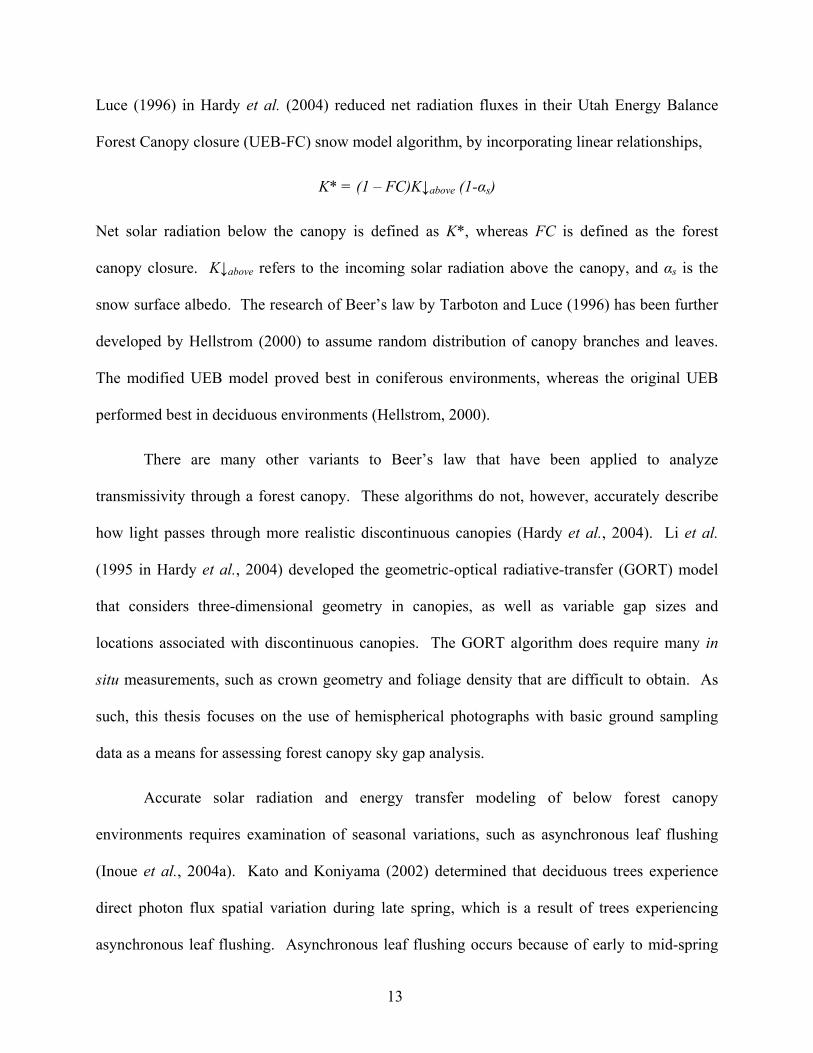
Luce (1996) in Hardy et al. (2004) reduced net radiation fluxes in their Utah Energy Balance

Forest Canopy closure (UEB-FC) snow model algorithm, by incorporating linear relationships,

K* = (1 – FC)K↓above (1-αs)

Net solar radiation below the canopy is defined as K*, whereas FC is defined as the forest

canopy closure. K↓above refers to the incoming solar radiation above the canopy, and αs is the

snow surface albedo. The research of Beer’s law by Tarboton and Luce (1996) has been further

developed by Hellstrom (2000) to assume random distribution of canopy branches and leaves.

The modified UEB model proved best in coniferous environments, whereas the original UEB

performed best in deciduous environments (Hellstrom, 2000).

There are many other variants to Beer’s law that have been applied to analyze

transmissivity through a forest canopy. These algorithms do not, however, accurately describe

how light passes through more realistic discontinuous canopies (Hardy et al., 2004). Li et al.

(1995 in Hardy et al., 2004) developed the geometric-optical radiative-transfer (GORT) model

that considers three-dimensional geometry in canopies, as well as variable gap sizes and

locations associated with discontinuous canopies. The GORT algorithm does require many in

situ measurements, such as crown geometry and foliage density that are difficult to obtain. As

such, this thesis focuses on the use of hemispherical photographs with basic ground sampling

data as a means for assessing forest canopy sky gap analysis.

Accurate solar radiation and energy transfer modeling of below forest canopy

environments requires examination of seasonal variations, such as asynchronous leaf flushing

(Inoue et al., 2004a). Kato and Koniyama (2002) determined that deciduous trees experience

direct photon flux spatial variation during late spring, which is a result of trees experiencing

asynchronous leaf flushing. Asynchronous leaf flushing occurs because of early to mid-spring

14

flushing trees nearing the end of their flushing stage, while late-spring flushing trees having just

begun their leaf flushing (Kato and Koniyama, 2002).

Understory trees frequently leaf flush before overstory trees, which may negatively

influence sky gap values derived from in situ remote sensing. Deciduous broad-leaved trees also

experience significant leaf phenology variation, as this forest characteristic is tree and tree-

species specific. This too can influence sky gap results, especially during the spring and fall

seasons.

Data collection involving forest components must then include any and all observed

changes to and within a forest and its canopy during data measurement. Forests are constantly

evolving at different spatial scales, and these changes vary based on environmental conditions,

human disturbance, physical appearance, individual tree type, forest type, forest size and forest

canopy (Gong and Xu, 2003). Forests at the stand scale experience changes to their canopies in

terms of both horizontal and vertical components. Horizontal components of a forest canopy

include changes in canopy closure, gap size and shape, whereas vertical components include the

number of layers and height of each layer in the understory.

MSC’s algorithm suite involves the collection of passive microwave remotely sensed

data. This type of remotely sensed data can be collected through both airborne and space-borne

platforms, and the use of data derived from passive microwave remote sensing is prone to issues

of scale. The issues and the research involved to correct it will be discussed.

2.3 Current State of Research for Passive Microwave Remote Sensing of Prairie SWE

Monitoring snow accumulation and depth in Canada can help prepare different

stakeholders about foreseeable droughts or flooding (Rango et al., 1983). Snow accumulation

and depth is important in monitoring water levels for many water-reliant activities because

15

snowmelt contributes in excess of 50% of the total annual discharge in many mountainous

regions, including Canada’s Rocky Mountains. Snow depth has two main purposes during the

winter months; (i) it acts as a source of stored water come spring runoff, and (ii) it acts as an

insulator protecting the soil and vegetation from winter elements. Monitoring SWE is important

for understanding the relationship between global climate change and Canada’s variable snow

accumulation, as well as helping to improve water conservation and preparedness practices

(Rango et al., 1983).

There are many Canadian organizations involved in climate change research and in the

development of functional remote sensing tools that can be applied to SWE data retrieval. The

SWE algorithm suite is one major Canadian contribution to understanding and monitoring

variable snow accumulation and depth in the form of SWE. The SWE algorithm suite is an

intensive passive microwave algorithm suite that makes use of passive microwave and in situ

data to obtain estimated SWE values for different vegetative structure regions in Canada.

Many scientists and researchers are involved in the development of the SWE algorithm

suite, with main co-ordinators including MSC’s Climate Research Branch, with Dr. Chris

Derksen focusing that branch’s efforts, with main research activities for the project spear-headed

by Dr. Ellsworth LeDrew at the University of Waterloo, Canadian Cryospheric Information

Network (CCIN), State of the Canadian Cryosphere (SOCC) and CRYospheric SYStem in

Canada (CRYSYS) (Figure 2.2).

16

Figure 1.2: Main Co-ordinators of SWE Algorithm Suite

Holistically, cryospheric research, including the development of MSC’s SWE algorithm suite,

affects climate change decision-making at the national and global levels. As such, citizens at

large are stakeholders when dealing with a national or global issue, like the cryosphere’s role in

climate change (Piwowar et al., 2002).

The algorithm suite makes use of passive microwave radiation, and the algorithms are

based on the “vertically polarized difference index for dual channels (19 and 37 GHz) of the

Special Sensor Microwave/Imager (SSM/I)” (Derksen et al., 2002a, pg. 1). The vertical

polarized difference is used because its accuracy with retrieving SWE is stronger than with the

horizontal polarized difference. The algorithm suite makes use of dual channels, or frequencies,

because the use of a single channel would make it more sensitive to changes in snow

characteristics (Derksen et al., 2002a; Goodison et al., 1994 in Derksen et al., 2000). The 37

GHz channel is a high scattering frequency, while the 19 GHz channel is a low scattering

frequency. The changes to microwave radiation scattering are caused by the presence of snow

crystals, and permit measuring ‘terrestrial SWE in the microwave portion of the electromagnetic

spectrum’ (Derksen et al., 2002, pg. 2).

17

The algorithm suite is comprised of four different SWE retrieval algorithms. As

previously mentioned, each algorithm represents a particular standing vegetative structure:

deciduous forest (FDSWED), coniferous forest (FCSWEC), sparse forest (FSSWES) and

open/prairie environments (FOSWEO). The algorithm suite is shown below:

SWE = FDSWED + FCSWEC + FSSWES + FOSWEO

(e.g. Derksen, 2002; Derksen et al., 2002a)

The final SWE value obtained from the algorithm suite represents a spatial location’s weighted

average derived from the proportion of standing vegetation structure within each pixel (Derksen

et al., 2002; Derksen et al., 2002a; 2002b). Characteristics of the remotely sensed data, such as

spatial resolution, and physical properties of the snow influence the SWE algorithm suite

performance (Derksen, 2002; Derksen et al., 2002).

A characteristic of passive microwave remotely sensed data that negatively impacts SWE

algorithm suite performance is its large pixel size. In order to obtain an accurate final weighted

SWE value based on the four standing vegetative structure algorithms and to effectively use

snow cover data for climate modeling, it is necessary for the passive microwave sensor to first be

able to interpret large scale vegetative structures (Derksen et al., 2000). The MSC are managing

this concern by developing their algorithm suite to take into account varying vegetative structure.

MSC synchronize the collection of ground snow pit data with the collection of their remotely

sensed passive microwave data. The collection of ground snow pit data is an example of using

large scale in situ data to ground-truth small scale remotely sensed data.

Howard (1991) recommends using large scale methods of remote sensing data retrieval

when assessing spatial variability as small scale remote sensing methods do not result in the

same usable data. Large scale spatial data used in ecological applications is frequently prone to

18

errors and biases during the analysis and decision making steps (Case and Fisher, 2001).

Uncertainty can relate to,

(i) absolute positions of features on the landscape;

(ii) type and characteristics of land cover;

(iii) shape of vegetation and its influence on neighbouring flora and fauna ecosystem

components;

(iv) importance of knowing spatial locations of different ecosystem components in

understanding different ecological processes; and

(v) how to weigh the importance of species and ecological processes in determining the

overall function of an ecosystem in address legislative priorities, such as addressing

global climate change.

Howard (1991) recommends that potential errors be addressed and documented so as to

minimize their influence on data analysis results.

In this thesis we examine and test digital in situ remote sensing as a means to obtain sky

gap estimates for a snow-covered predominantly coniferous environment. In this chapter we

address the utility of a type of in situ remote sensing, hemispherical photography, in assessing

forest stands at the canopy scale for accounting of vegetative structure during SWE analysis

undertaken at the passive microwave scale.

2.4 Current State of Research for In-situ Remote Sensing of Forest Environments In situ remote sensing of forest environments provides the framework for measuring

forest attributes of all scales (Fournier et al., 2003). Culvenor (2003) highlights that the choice

of spatial resolution of the remote sensing platform is dependent on the subject matter, and

choice of the platform determines the quality of information obtained. Hemispherical

19

photography permits the analysis of individual forest stands, which results in this type of data

being referred to as having a high spatial resolution (Culvenor, 2003).

Hemispherical canopy photography involves the use of a hemispherical, or ‘fish-eye’,

lens with a field of view (FOV) approaching or near 180-degrees, and taking a picture while

looking up at the tree canopy. Hemispherical photography is a passive indirect optical means of

obtaining information about numerous tree canopy characteristics, including canopy gaps (sky

gap analysis), LAI (Leaf Area Index) and transmittance (e.g. Hale and Edwards, 2002; Rich,

1990).

Passive indirect optical measurement methods, unlike active methods, measures the

interaction between the forest canopy and solar radiation during documented weather conditions,

and the information is then used to determine structural characteristics of the forest canopy

(Fournier et al., 2003). Canopy gap size, position and distribution can be measured through the

use of hemispherical photography, or by determining the proportion of beam or diffuse light

transmitting through the forest canopy (Fournier et al., 2003). Indirect measurements of a forest

canopy can complement additional datasets, and act as an alternative data source in locations

without direct datasets (Fournier et al., 2003). Indirect measurements frequently provide a cost-

effective option for more frequent or complimentary data retrieval.

Hemispherical canopy photography is considered a suitable ground-based (in situ) remote

sensing tool for indirectly measuring forest canopy architecture and light interception. Fournier

et al. (2003) summarized five main advantages that the use of hemispherical photography has

over alternative optical methods for in situ sky gap analysis:

20

(i) camera settings allow for photographic adjustments to compensate for errors arising from variations in transmittance;

(ii) spatial information is permanently stored in the image;

(iii) provides a means for analyzing LAI at the canopy level;

(iv) provides a visual aid for the interpretation of canopy attributes and structure; and

(v) is an alternative for when weather and sky conditions do not permit data acquisition from other techniques.

Hemispherical canopy photography may be taken facing upwards from below a canopy, or

facing downwards from above the canopy (Fournier et al., 1996; 1997, Herbert, 1987; Rich,

1990). If facing upwards from below the forest canopy, a circular image is produced that

presents the zenith in the center with the image edges showing the horizon. Hemispherical

canopy photography makes use of an extreme wide-angle sensor (the camera with a

hemispherical lens) to measure light transmission, and the resultant sky gap analysis reflects the

“size, shape, and location of gaps in the forest” canopy so as to obtain an instantaneous

measurement of the forest canopy structure (Fournier et al., 2003; Frazer et al., 1999, pg. 1;

Anderson, 1964 in Rich, 1990).

Hemispherical photography assesses variation in vegetation on a local scale, making this

indirect measurement technique sensitive to small variations in the forest canopy. This

sensitivity to changes in forest canopy make hemispherical canopy photography an inexpensive

alternative to light sensors, such as radiometers, which can directly assess light measurements

underneath the forest canopy at a specific point and time, but requires costly maintenance (Inoue

et al., 2004a).

Canham and Burbank (1994) and Herbert (1987) detail standard procedures for

producing hemispherical photographs so that outside variables, such as height above the ground

in which the photographs are taken, are constant. The need for a photograph procedure is

important because small inconsistencies arising from, for example, varying photograph height

21

may result in contradictory results, while angular distortions can result in large changes to the

hemispherical object region (i.e., the forest area that is displayed in the hemispherical

photograph) (Herbert, 1987). Angular distortions occur when the base of hemispherical

photography platform is not horizontal to the study site.

Inoue et al. (2004a; 2004b) describe their photograph procedure as including mounting

the digital camera with hemispherical lens on a tripod at a height of 1.2 metres above ground.

The camera platform was then made flush with horizontal using a bubble level. Automatic

camera settings for aperture width and shutter speed were also used to minimize time delay

between photographs (Englund et al., 2000).

Awareness of the type of lens projection permits the understanding of radial lens

distortion. Hemispherical lenses have object regions of “equal solid angle [that] do not result in

images of equal area” (Herbert, 1987). Instead, the object region is projected, resulting in a

radial lens distortion, because the region area is a function of the angle between the lens’ optical

axis and the object region center. Herbert (1987) determined that even a very small amount of

radial lens distortion results in substantial changes to the projected area on the hemispherical

photograph plane.

It is important to understand how the hemispherical object region is displayed as there are

four main types of hemispherical lens projections: polar, orthographic, stereographic, and

Lambert’s Equal Area (Frazer et al., 1999). Miyamoto (1964 in Herbert 1987) summarized the

influence of the four main hemispherical projections by examining how a point on a hemisphere

can be examined by its azimuthal angle α, and zenith angle ζ. The radial projection of a point

was examined by how the projection influenced its location on a circular disk with radius π/2

22

with final polar coordinates α', and zenith angle ζ', where 0 ≤ ζ ≤ π/2 and 0 ≤ ζ' ≤ π/2. The four

radial projections are further described by Miyamoto (1965 in Herbert, 1987) in Table 2.3.

Table 2.3: Radial Projection Characteristics

Projection Type Radial Projection Characteristics Polar ζ' = ζ Orthographic ζ' = (π/2)sin(ζ) Stereographic ζ' = (π/2)tan(ζ/2) Lambert’s ζ' = (π/√2)sin(ζ/2)

The Lambert projection is useful in ecological studies as it preserves areas during the transfer of

information from the object area to the projected area. The stereographic projection preserves

angles between arcs of great circles, whereas the orthographic projection displays points in a

normal direction to the projected area. Most common hemispherical lenses have, however, a

polar projection, which is neither equal area nor equal angle.

Additional procedures recommended by Canham and Burbank (1994) and Herbert (1987)

include ensuring (i) that the photographs are taken perfectly horizontal (i.e., without the camera

tilted), and (ii) that the lens and camera calibration remain consistent for all hemispherical

photographs in a study. It is also recommended that the hemispherical lens’ FOV be positioned

towards the north compass direction to meet software requirements that request the user to

indicate where the compass directions are on the image (Rich, 1990; Frazer et al., 1999).

Hemispherical photographs of forest canopies can be recorded using two different forms

of photography: film and digital. Digital hemispherical photography provide an added incentive

of being able to visually check and redo photographs while in the field, and have an added bonus

during temporal studies on light environments as they do not require film processing and image

scanning (Hale and Edwards, 2002; Inoue et al., 2004a).

23

Inoue et al. (2004a) summarize that digital hemispherical photography is an effective tool

for studying light environments beneath a forest canopy as they may be more sensitive than film

photography in recording light reflecting off of forest canopy features, such as leaves. This

increased sensitivity may, however, result in occasional overestimation of light in digital

hemispherical photographs (Englund et al., 2000). To avoid misinterpretation of data derived

from digital or film photographs, Inoue et al. (2004b) suggest indicating the platform used.

Specifying the platform also permits comparing data results obtained from a different digital

camera.

Hale and Edwards (2002) compared the utility of film and digital hemispherical

photography and determined strong positive correlation between the two mediums over a

transmittance range of 10 to 70%. Film and digital hemispherical photographs do, however,

produce variable transmittance values below very dense canopies (transmittance greater than

10%), with digital hemispherical photographs reporting higher estimates of transmittance, and

corresponding estimates of LAI are generally lower. Research findings are, however, conflicting

on whether hemispherical photography, in either film or digital format, can discriminate

transmittance levels in dense canopies (where transmittance is between 5-10%) (Hale and

Edwards, 2002).

In the comparison of digital and film hemispherical photography undertaken by Englund

et al. (2000), it was highlighted that some of the differences between the many hemispherical

photograph platforms could be attributed to the view angle and distortion of the hemispherical

lenses used. The Nikon FC-E8 hemispherical lens, for instance, has a FOV greater than the

expected 180° (Inoue et al., 2004a). The FC-E8’s FOV of 183° resulted in a systemic error

which will be addressed in Chapter 4.

24

Frazer et al. (2001) examined the utility of a consumer-grade inexpensive digital camera

in obtaining hemispherical photographs for use in scientific inquiry. Hemispherical

photography, either film or digital, should be set for underexposure, as this has frequently

provided the best contrast between the sky and canopy (Hale and Edwards, 2002; Chen et al.,

1991). Underexposure is typically set on the camera by ½ and 1 f-stop. On digital cameras,

image quality (compression) has been found to not significantly impact the photograph or

extraction of data from it (Hale and Edwards, 2002; Englund et al., 2000).

Frazer et al. (2001) compared the Nikon Coolpix 950 with Nikon FC-E8 hemispherical

converter, which is the same system used during the retrieval of hemispherical photographs for

this thesis, along side a film camera, and determined that the digital camera system frequently

produced canopy photographs with significant colour blurring along the outer fringe of the

photo. Colour blurring, or chromatic aberration, on digital hemispherical photographs negatively

influence the photos and much of the analysis completed on them. Frazer et al. (2001) has

summarized how chromatic aberration of hemispherical photographs can impact the data

obtained through the use of the Nikon Coolpix 950 with FC-E8 hemispherical converter

platform, and their findings are included below:

(i) the size, shape, and distribution of canopy gaps vary;

(ii) the accuracy of edge detection and the binary division of pixels into sky and

canopy elements are negatively impacted; and

(iii) the magnitude, range and replication of canopy openness, leaf area, and

transmitted global radiation results are negatively impacted.

Setting the Nikon Coolpix 950 to record photographs in black and white, and taking the

photographs under uniformly overcast weather conditions help to minimize the negative impacts

25

caused by the chromatic aberration. Englund et al. (2000) highlights that the conveniences of

digital photographs first outlined by Hale and Edwards (2002) and Inoue et al. (2004a),

combined with the cost savings from not having to develop film outweighed any disadvantages

observed from image quality.

Inoue et al. (2004a) examined the use of digital hemispherical photographs from two

different Coolpix camera suites; Coolpix 900 and Coolpix 990. Inoue et al. (2004) determined

that changing the image quality to any of the three image quality settings - basic, normal and fine

- did not result in any significant variations between hemispherical photograph-derived gap

fraction estimates. Changes to the image quality (basic, normal, fine and high) in the Nikon

Coolpix 950 with FC-E8 hemispherical converter does not greatly impact data derived from the

photographs, such as sky gap, and thus basic image quality is sufficient (Englund et al., 2000;

Inoue et al., 2004a; Frazer et al., 2001).

Inoue et al. (2004a) did determine that changing the image size setting on the Coolpix

900 and 990 cameras resulted in notable variations between hemispherical photograph-derived

sky gap estimates. Sky gap estimates were lower in full-size images than with VGA-size images:

full-size images have a higher pixel resolution than VGA-size images. Inoue et al. (2004a)

suggest using full-size images as these images can better capture full canopy structure, including

smaller branches, leaves and needles. Inoue et al. (2004a) made use of hemispherical

photographs Frazer et al. (2001) obtained using a Coolpix 950 camera with a Nikon FC-E8

hemispherical lens, and compared their results to those obtained on either the Coolpix 900 or 990

platforms. Inoue et al. (2004a) determined that derived sky gap estimates using the Coolpix 950

platform were opposite to those obtained on the 900 or 950 platforms. The Coolpix 950 derived

sky gap estimates were lower in VGA and XGA-size images than in the higher resolution full-

26

size (FINE) images, but that these variations do not greatly influence data derived from FC-E8

hemispherical photographs (Inoue et al., 2002 in Inoue et al., 2004a).

Many of the differences Inoue et al. (2004a) and Frazer et al. (2001) observed in their

derived-sky gap results, such as the ability to capture full canopy structure were due to variations

in the effective pixel count of the camera, which varies from camera to camera. The Coolpix

990 camera has a higher effective pixel count than the Coolpix 900, 3.14 million pixels to 1.22

million pixels, whereas the Coolpix 950 has an effective pixel count of 1.92 million pixels

(Nikon [oregonstate.edu/mediaservices/classup/manuals/cp950rm.pdf] February, 2007). The

writer recognizes that the Coolpix 950 does not have the highest effective pixel count currently

technologically available, but this model was available for use and the effectiveness of the

Coolpix cameras have mainly been documented in deciduous environments; however, in this

thesis we examine mixed wood to coniferous type environments.

The Nikon FC-E8 hemispherical converter used in this thesis provides a simple polar

projection (Herbert, 1987; Inoue et al., 2004a). Inoue et al. (2004a) addressed lens distortion in

the FC-E8, and obtained unpublished data from the Electric Image Technical Center of Nikon,

which Inoue et al. then used to develop a calibration to compensate for the lens distortion. In

comparing data derived from hemispherical photographs with lens distortion and from calibrated

hemispherical photographs, Inoue el al. noted a positive correlation between calibrated and

uncalibrated -derived canopy cover and weighted openness values, although both slope and

intercept of the regression line between the two datasets were comparatively different.

Inoue et al. (2004a) hypothesized that their research into the differences between

calibrated and uncalibrated hemispherical photographs highlights that there must be other factors

27

acting on the differences between film and digital hemispherical photograph-derived data. These

differences may instead arise from, for example, light sensitivity and sky condition.

Ishida (2004) summarized the utility of digital hemispherical photography in different

forest conditions, and states that this type of data retrieval is best suited for open areas and at

forest edges, but is prone to overestimating canopy in dense forests. Hemispherical photography

is also best suited for areas with minimal slope. Slope impacts the collection of hemispherical

photography as gap algorithms and software are not typically designed to factor in changes in

forest path length caused by a slope (Fournier et al., 2003). Forest canopy facing upslope in

hemispherical photographs appear dense with small canopy gaps, while forest canopy facing

downslope appears open with large canopy gaps.

Hemispherical photographs are instantaneous measurements of the forest canopy. As a

result, derived-sky gap values are instantaneous as well. It is ideal to sample the light

environment of forest floors over an extended period of time, such as over numerous days, to

further understand light’s spatial and temporal differences. Measuring the below canopy light

environment for an extended period of time is, unfortunately, unfeasible or impractical for most

research missions (Gendron et al., 1998). More practically, it is suggested to take instantaneous

light measurements on overcast days when the solar radiation is in the form of diffuse light,

which can be considered stable throughout the day thus reducing spatial variability (Messier and

Puttonen, 1995 in Gendron et al., 1998; Gendron et al., 1998).

Minimal spatial variability can, however, hinder contrast between the sky and vegetation

(Gendron et al., 1998). Anderson (1964) suggests taking instantaneous measurements both

inside and outside the forest canopy to account for diffuse light differences. Weather conditions

such as full sun and part-sun may result in the short-term fluctuations of light. On part-sun days,

28

light conditions may be experience variations from clouds and diffuse light from the sky

(Anderson, 1964).

There are many variables that should be addressed when designing a procedure involving

the collection of in situ hemispherical photographs. These variables include, but are not limited

to, deciding on film type; camera settings; type of radial projection to use; weather preference

and need (or lack thereof) of constant outside variables (camera height, etc.). Variables that need

addressing may also depend on how the collected hemispherical photographs will be analyzed.

2.5 Current State of Research for Analyzing Hemispherical Photographs Rich (1990) outlines two methods of analyzing hemispherical canopy photographs: by

hand and digitally. Hand analysis is described as extremely tedious and impractical for

analyzing many hemispherical photographs in a short period of time, and in this thesis we will

therefore focus on digital image analysis. Hale and Edwards (2002) used Hemiview© (Delta-T

Devices, Cambridge, UK) to calculate canopy openness, diffuse and direct transmittance, and

LAI. Hemiview provides settings for different lenses, which allows the user to compensate for

differences derived from lens distortion. The use of software to analyze hemispherical

photographs uses a threshold value to differentiate between sky and canopy elements, thus

eliminating any human subjectivity that traditionally influenced the results for both sky gap and

canopy cover analyses (Anderson, 1964 in Ishida, 2004).

GLI/C© (Gap Light Index) and GLA© (Gap Light Analyzer) are two separate software

suites that can be used for analyzing hemispherical photographs. Both were created with the

assistance of Dr. Charles Canham from the Institute of Ecosystem Studies (Millbrook, New

York, USA). GLI/C is the predecessor to GLA, and has fewer options than GLA, and makes use

of the GLI algorithm, which calculates the %PAR (Photosynthetically Active Radiation)

29

transmitted through a canopy gap to any location in the forest understory over a growing season

(Canham, 1988). The GLI algorithm assumes there is a correlation between the size and shape

of a canopy gap with the beam (direct) and diffuse (indirect) transmission of light to a location

within or near the gap. The GLI algorithm is shown below:

GLI = [(TdiffusePdiffuse) + (TbeamPbeam)] · 100.0

(Canham, 1988)

Seasonal PAR received at the top of the forest canopy is illustrated in the algorithm as diffuse

PAR (Pdiffuse) or beam PAR (Pbeam), where diffuse PAR can be calculated as,

Pdiffuse = 1 - Pbeam

The proportion of diffuse and direct PAR that is transmitted through the canopy to a position in

the understory is shown as Tdiffuse and Tbeam. Values computed through the use of this algorithm

range from 0, which occurs when no defined canopy gap is present, to an open site with a value

of 100 (Canham, 1988). An atmospheric transmission coefficient (KT) is available for the GLI

algorithm, and accounts for seasonal variations in the amount of atmospheric incident solar

radiation transmitted to the earth’s surface. The coefficient value and direct PAR (Pbeam), have a

positive correlation. Thus as the amount of beam PAR increases for the instantaneous

measurement site, so does the value of the coefficient, and as the coefficient value decreases so

does the amount of beam PAR. The coefficient has more utility when studying deciduous forest

canopy sky gap where the growing season and annual seasons will have varying sky gap values

(Canham, 1988).

In comparison, GLA permits the user to set, for example, the solar time; sky-brightness

model; inclination angle of the hemispherical lens, in addition to adding a different projection or

30

distortion model. The correlation of results between GLI/C and GLA is dependent on the user’s

adjustments of GLA’s added features. The GLA User Manual (Frazer et al., 1999) states that

GLA’s added feature of setting the solar time allows the software to more accurately compute

beam transmission through canopy gaps by checking to see if pixels in the digital photograph are

open or closed based on the sun’s position at a particular time in the day. The sun’s position can

either be obstructed by the canopy, which results in a direct radiation value of zero, or it can be

directly overhead, which results in a direct radiation value equal to the above-canopy radiation

value (Hardy et al., 2004). Solar beam enrichment from either scattered and/or reflected

radiation is not considered in the GLI algorithm.

User-supplied variables for the GLA Software include both measured and assumed

values, and a general description of these variables is from the GLA Version 2.0 User Manual

and Program Documentation, and Hardy et al. (2004). User variables include a cloudiness index

(ranges from 0 to 1), image orientation (slope and aspect of the study site), custom hemispherical

lens projection transformation, site location (inclusion of latitude, longitude and elevation for the

study site), solar time step (measured in minutes), sky region (regions within the sky hemisphere

used to attempt to model diffuse-light transmission), and dates of field study.

GLA provides a range of output data on analyzed hemispherical photographs. Output

data is in tabular format, and involves key information such as % Canopy Openness values. In

this thesis we interpret GLA’s % Canopy Openness Values derived from the hemispherical

photographs as instantaneous sky gap estimates. The objective of this thesis is to test and

examine the utility of a type of in situ remote sensing, hemispherical photography, as a means of

obtaining sky gap estimates for use in forest and remote sensing studies. The motivating

application for this thesis is to find a correction factor that will account for vegetative structure

31

when using passive microwave data in snow-covered predominantly coniferous environments.

Experiment procedure and GLA output data will be addressed further in Chapter 3.

32

CHAPTER THREE: Methodology

3.1 Introduction The purpose of this research is to examine and test the use of hemispherical photography

as a means for obtaining in situ sky gap estimates in a snow-covered boreal forest. The

collection of hemispherical photographs is a method for obtaining in situ sky gap estimates

concerning forest canopy structure to correct the issue of scale in deriving SWE values from

passive microwave data. Hemispherical photography is a means for collecting large scale data,

which permits assessment of vegetative structure at the local level.

In this research we identify four components to data collection: weather and radiation

data for the field sites on field days, snow pit data for hemispherical photograph test sites, visual

interpretation of vegetation structure in the form of field notes surrounding snow pit sites, and

hemispherical photographs for each snow pit site. The four data collection components are

intended to ensure that procedures recommended by hemispherical photographer researchers is

followed (see Fournier et al., 2003 and Inoue et al., 2004a, etc.), and to ensure that requirements

of the GLA software are met.

The framework adopted in this thesis requires that sky gap data be extracted from digital

hemispherical photographs of forest canopy. The procedure and apparatus for collecting digital

hemispherical photographs used in this research was determined as a result of experience gained

during previous collaborative SWE data collection experiments lead by the MSC. These two

winter field experiments involved the collection of multi-scale data, including both space-borne

and airborne remotely sensed passive microwave data, as well as extensive temporally-

coincident ground samples (Derksen, 2002).

33

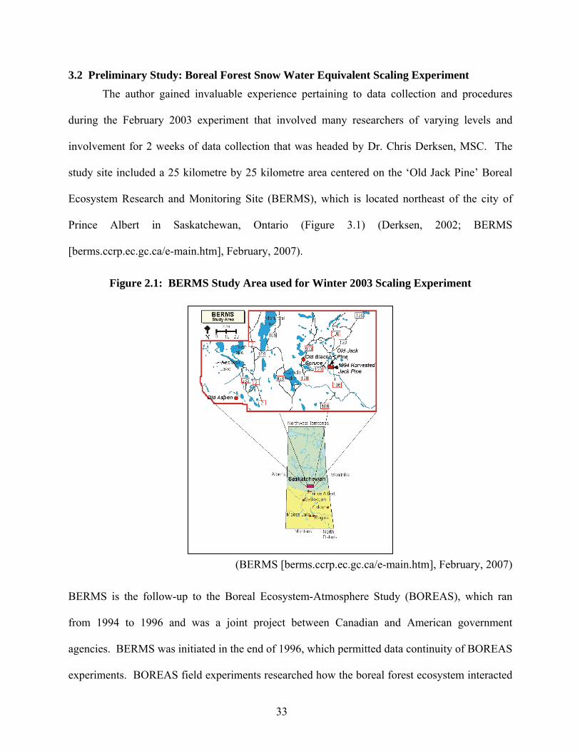
3.2 Preliminary Study: Boreal Forest Snow Water Equivalent Scaling Experiment The author gained invaluable experience pertaining to data collection and procedures

during the February 2003 experiment that involved many researchers of varying levels and

involvement for 2 weeks of data collection that was headed by Dr. Chris Derksen, MSC. The

study site included a 25 kilometre by 25 kilometre area centered on the ‘Old Jack Pine’ Boreal

Ecosystem Research and Monitoring Site (BERMS), which is located northeast of the city of

Prince Albert in Saskatchewan, Ontario (Figure 3.1) (Derksen, 2002; BERMS

[berms.ccrp.ec.gc.ca/e-main.htm], February, 2007).

Figure 2.1: BERMS Study Area used for Winter 2003 Scaling Experiment

(BERMS [berms.ccrp.ec.gc.ca/e-main.htm], February, 2007)

BERMS is the follow-up to the Boreal Ecosystem-Atmosphere Study (BOREAS), which ran

from 1994 to 1996 and was a joint project between Canadian and American government

agencies. BERMS was initiated in the end of 1996, which permitted data continuity of BOREAS

experiments. BOREAS field experiments researched how the boreal forest ecosystem interacted

34

with the “atmosphere in relation to climate change”, whereas a focus of BERMS is to obtain data

and information to help define the current global carbon dioxide (CO2) budget (BERMS

[berms.ccrp.ec.gc.ca/e-main.htm], February, 2007).

BERMS is located in the southern fringe of the boreal forest, and has many qualities ideal to

the research objectives of examining issues related to the development of the boreal SWE

algorithm, including:

• variety of coniferous species; • range in vegetation age, structure and resultant size; • environmental changes associated with human activities (i.e. logging and forest

maintenance practices); • pre-existing instrument towers from BERMS and BOREAS field experiments; and • pre-existing remotely sensed and ground sampling data from both BERMS and BOREAS

field experiments.

The author was involved in collecting snow pit data, snow crystal macro-photography and

hemispherical photography of the canopy cover. The hemispherical photographs collected

during the winter 2003 field experiment had many sampling errors introduced as a result of

inconsistencies regarding how the camera was set-up to take each photograph at the different

snow pit sites, and from periodic electronic and battery failure during the experiment resulting

from prolonged exposure to extreme cold temperatures (i.e., temperatures approaching -48°C).

The collection of hemispherical photographs was part of an auxiliary dataset, and an

apparatus such as a tripod was not utilized as there was no means to transport it along with more

important snow pit measuring devices while traversing on-foot along different snow courses.

A sample hemispherical photograph from the winter 2003 experiment is shown in Figure 3.2.

35

Figure 3.2: Sample Problematic Hemispherical Photograph from Winter 2003 Experiment

© Diane Redekop, 2003

Problems with the winter 2003 hemispherical photograph set that are visible in Figure 3.2

include the unidentified angle from the horizontal the photograph was taken from, in addition to

capturing the author’s hat and fellow researcher in the image. Additional inconsistencies in the

2003 hemispherical photograph dataset include not knowing the height above ground surface that

the images were taken at, as well as not standardizing the compass directions on the images. The

listed inconsistencies, as well as the sun’s low position and clear skies create problems with the

GLA software and do not follow the recommendations set by Anderson (1964) to obtain these

images under cloudy conditions. To meet the data needs of this experiment, a second experiment

was designed that prioritized the collection of hemispherical photography.

36

3.3 Secondary Study: February 2004 MSC Experiment The two-day MSC experiment in February 2004 was headed by Ms. Anne Walker, MSC,

and involved both professional and student researchers from the University of Waterloo to

collect ground snow pit data to aid in calibrating temporally co-incident airborne microwave

SWE data. The goal of the experiment, like the February 2003 experiment, was to help in the

development of MSC’s SWE Algorithm Suite, and in particular, to examine how vegetative

structure influences algorithm performance. This experiment used different farm fields and an

Agreement Forest located in the Region of Waterloo, Ontario, to collect snow course data that

followed the flight lines used to collect MSC’s airborne microwave data.

The author gained additional experience in snow pit data collection, as well as in

experiment planning and execution. As a result, the author made use of her familiarity with the

Waterloo Region Agreement Forest used during the February 2004 MSC Experiment to

coordinate a hemispherical photograph field experiment with corresponding snow pit data.

3.4 Thesis Study: February 2004 Hemispherical Photography Experiment The author made use of a modified-version of a digital hemispherical photography

collection procedure described by Gong and Xu (2003) during the February 2004 field

experiment (Figure 3.3). This 5 step experiment procedure begins with in situ hemispherical

photography data collection and auxiliary snow pit data, which will be followed with image

preprocessing using Adobe Photoshop 7.0, which will then be followed by image processing

using Gap Light Analyzer Version 2.0 and data analysis using Microsoft Office XP Excel.

37

Figure 3.3: Procedures in a Digital Photography Derived Sky Gap Estimates Task

Raw hemispherical photographs were collected during a one-day experiment performed

on February 19, 2004 with the aid of Mr. Gerry McIsaac, a student researcher who also

participated in the February 2004 MSC Experiment. Unlike previous snow experiments, data

priority during this experiment focused on the collection of hemispherical photography in a

boreal forest-like environment with snow pit data being complimentary. The sample size of

collected hemispherical photographs was restricted by, for instance, field experiment duration,

which was limited to one day because of logistical and weather reasons. Additionally, some of

the hemispherical photographs collected were not suitable for use during data analysis, and is

further described in section 4.2.

The 2004 Hemispherical Photography Experiment was completed at the Macton

Agreement Forest (Figure 3.4: Map and Airphoto of Macton Agreement Forest), which is a

forest stand owned and managed by the Region of Waterloo and formerly managed by the

Ministry of Natural Resource. For the purposes of this thesis, a forest stand refers to an

aggregation of trees with uniform composition making it distinguishable from nearby crops

Raw Image Collection

Image Preprocessing

Image Registration in

Software

Derived Sky Gap Estimates

Image Processing

38

(Howard, 1991). Macton Agreement Forest is located in the Township of Wellesley at the

southwest corner of Highway 86 and Manser Road (also known as Highway 19/Perth Road 131)

in the Region of Waterloo.

39

Figure 3.4: Map and Airphoto of Macton Agreement Forest

Macton Agreement Forest is bordered by Highway 86 to the north, Manser Road to the east and

barren fields to the south and west. There is understory and fringe deciduous tree growth with

periodic mixed tree environment open areas in the Agreement Forest (Figure 3.5).

© Region of Waterloo Locator [locator.region.waterloo.on.ca], 2007

Colour ortho-imagery taken in 2006 with 30 centimetre resolution.

Macton Agreement Forest

40

Figure 3.5: Macton Agreement Forest

The older coniferous trees in the Agreement Forest appear to have been planted as they are in

rows, and some rows appear to have been logged. New undergrowth is a variation of both

coniferous and deciduous trees. Figures 3.6 and 3.7 provide photographic detail of the

Agreement Forest’s vegetative structure and visible management history.


Picture taken facing south on the west side of Manser Road.

41

Figure 3.6: Macton Agreement Forest – Sample Vegetative Structure

Figure 3.7: Macton Agreement Forest – Sample Management History

The Agreement Forest, with its planted and logged history is characteristic of many coniferous

environments in Canada’s boreal region as they too frequently undergo forestry management

practices, including different types of logging and (re)planting practices. As a result, the

Tree planting in Forest was completed in what appears to be rows. Logging of the Forest is both scattered and sectional (in rows).



42

Agreement Forest is considered a suitable example of a coniferous environment for the purposes

of this thesis. Test sites were selected to represent a range of canopy openness – closed canopy,

gaps of various sizes and open canopy (Gendron et al., 1998). Sites were also chosen based on

depth of snow below the canopy (i.e., deep snow cover and shallow snow cover)

3.5 Sensor Platform Preparation Hemispherical photographs were captured using a Nikon Coolpix 950 digital camera and

a Nikon FC-E8 hemispherical converter that were mounted to a standard tripod. Figure 3.8

illustrates how experimental errors were reduced by having the base of the camera platform

consistently 1 metre from the earth’s surface. This was done by manually shoveling a ground

area clear of snow cover. The shoveled area doubled as a snow pit site where snow depth,

density, temperature and site characteristics were observed. Auxiliary data from the University

of Waterloo weather station for the day was obtained from their website [weather.uwaterloo.ca]

to compliment site information. A standard measuring tape ensured 1 metre distance between

the earth’s surface and top of the hemispherical converter.

43

Figure 3.8: Hemispherical Photograph Experiment Design

The camera platform was flush with the horizontal using a standard wood-working level that also

permitted angling the camera and hemispherical converter a consistent degree away from

horizontal. Additionally, each of the three tripod legs could be adjusted for length depending on

the topography of the forest floor. A compass aligned with the camera acted to ensure that north

on each image was identified. North direction was at the bottom of each image. All images

were taken using automatic camera settings, and saved in .JPG format at full image resolution

(1600 x 1200 pixels) and in normal (medium) quality image compression. The FC-E8 fisheye

lens has two modes: circular and full frame. Images were taken in circular mode for use in sky

gap analysis (requirement of GLA software).

© Diane Redekop and Jefferson Stephens, 2007 © Nikon [http://oregonstate.edu/mediaservices/classup/manuals/cp950rm.pdf], 2007

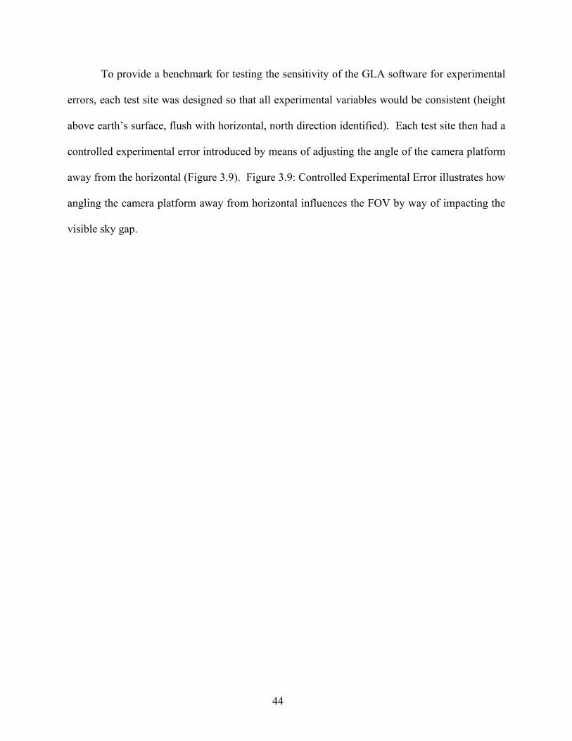
44

To provide a benchmark for testing the sensitivity of the GLA software for experimental

errors, each test site was designed so that all experimental variables would be consistent (height

above earth’s surface, flush with horizontal, north direction identified). Each test site then had a

controlled experimental error introduced by means of adjusting the angle of the camera platform

away from the horizontal (Figure 3.9). Figure 3.9: Controlled Experimental Error illustrates how

angling the camera platform away from horizontal influences the FOV by way of impacting the

visible sky gap.

45

Figure 3.9: Controlled Experimental Error (Population 1)


0º from horizontal © Diane Redekop, 2004

5º from horizontal


10º from horizontal



Angling the camera platform was done using the wood-working level at intervals of 0°

(horizontal), 5°, 10° and 20° from the horizontal, and the approximate centre of the

hemispherical lens was used as a guideline for measuring camera platform height of 1 metre

above the ground surface. While taking the photographs, the author and student crouched

underneath the platform and are not visible on any of the hemispherical photographs.

46

Hemispherical photographs were downloaded directly from the Nikon Coolpix 950 to a

personal computer. Hemispherical photographs were categorized based on test site and angle

from horizontal. The first test site was labeled as “A” with its four angled photographs being

A_0.jpg, A_5.jpg, A_10.jpg and A_20.jpg. Two identical copies of the original (raw) labeled

photographs were created and saved in separate folders. Three populations of photographs were

created using the raw photos and two copies, and are described in Table 3.1: Description of Data

Populations.

Table 3.1: Description of Data Populations

Population Main Description Modification Description Population 1 Raw Data No modifications made Population 2 Modified Framed Image Ground area around image

perimeter cropped out using Adobe Photoshop© 7.0

Population 3 Modified Threshold in GLA GLA© default threshold changed from 128 to 100

All 3 Population datasets of digital hemispherical images were analyzed using Gap Light

Analyzer© (GLA), Version 2.0, developed by the Institute of Ecosystem Studies at Simon Fraser

University, which is available on the Internet at http://www.ecostudies.org/gla/. Population 1

was left unmodified and there was no interactive thresholding of the photographs, as this is

frequently accompanied with observer bias and variation, caused by observer subjectivity (Inoue

et al., 2004a).

Population 2: Modified Framed Image had the black portions surrounding the image

removed in addition to cropping out the ground (snow area) around each of the images. This

step was completed to test for processing error in the GLA software. Snow and sky areas both

have high brightness values, and removing snow area from the image will be used to assess if the

software can differentiate between snow and sky brightness values when calculating sky gap.

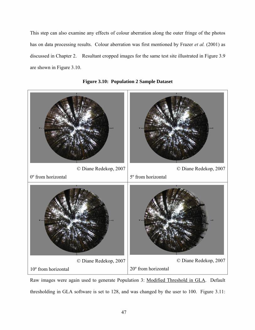
47

This step can also examine any effects of colour aberration along the outer fringe of the photos

has on data processing results. Colour aberration was first mentioned by Frazer et al. (2001) as

discussed in Chapter 2. Resultant cropped images for the same test site illustrated in Figure 3.9

are shown in Figure 3.10.

Figure 3.10: Population 2 Sample Dataset


0º from horizontal


5º from horizontal





Raw images were again used to generate Population 3: Modified Threshold in GLA. Default

thresholding in GLA software is set to 128, and was changed by the user to 100. Figure 3.11:

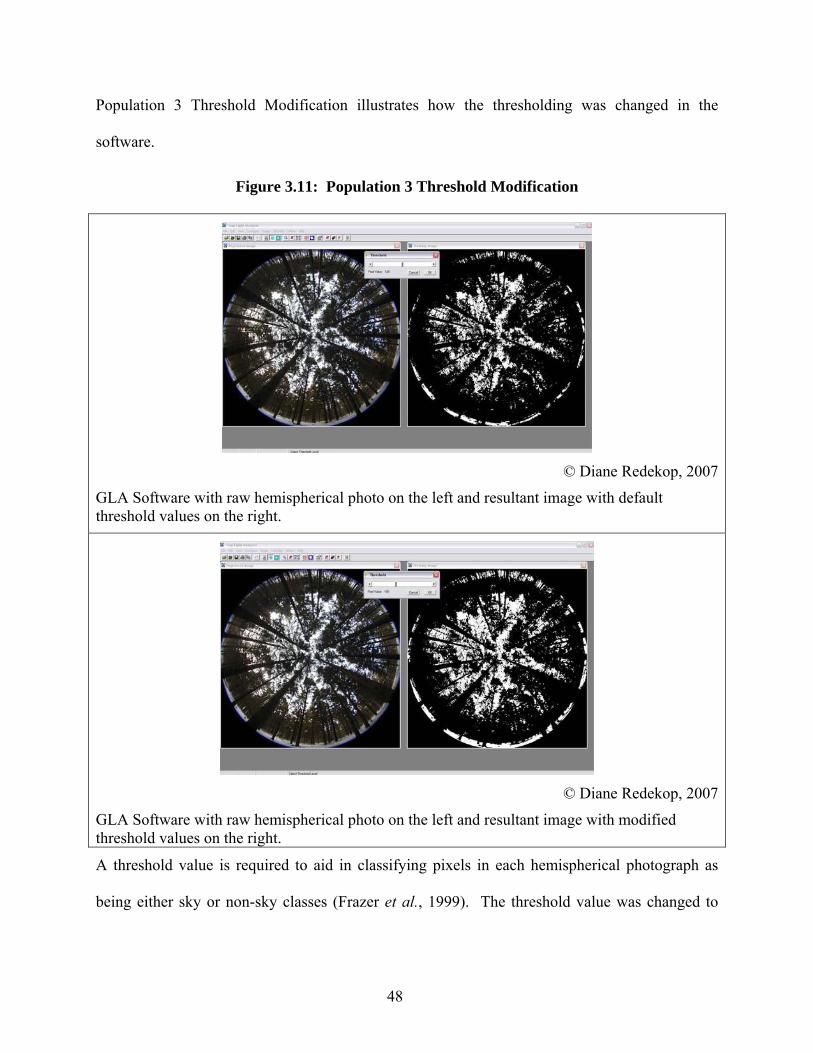
48

Population 3 Threshold Modification illustrates how the thresholding was changed in the

software.

Figure 3.11: Population 3 Threshold Modification


GLA Software with raw hemispherical photo on the left and resultant image with default threshold values on the right.


GLA Software with raw hemispherical photo on the left and resultant image with modified threshold values on the right.

A threshold value is required to aid in classifying pixels in each hemispherical photograph as

being either sky or non-sky classes (Frazer et al., 1999). The threshold value was changed to

49

100, instead of any other value because this modification resulted in noticeable, but not

exaggerated, change to the classified image.

Threshold values that were changed to values further away from the default threshold

values resulted in exaggerated classifications, while threshold values changed to values closer to

the default value resulted in barely noticeable changes. Additionally, a threshold setting of 100

was chosen because the true-colour image bright spot was blue sky (and not pure white),

therefore the median default threshold in GLA of 128 was not applicable to the images used in

this thesis. Threshold values less than the user-specified 100 resulted in fine-detail tree canopy

and partially snow-covered fallen branches and brush being reclassified as snow/sky. Threshold

values much greater than the user-specified 128 (threshold value of approximately 156+) result

in small sky gaps and small clusters of surface snow being reclassified as canopy.

The hemispherical photographs in Population 3 were themselves unmodified. Instead an

input (threshold) value for computing sky gap (% Canopy Openness) was altered from a default

setting in the GLA software to user-specified. This step was completed to test for software

sensitivity and processing error from modifying the default threshold values.

3.6 Analysis

GLA provides a range of output data on analyzed hemispherical photographs. A

calculation pertinent to this thesis includes percentage of canopy openness (% Canopy Openness)

for every hemispherical photograph in each of the three populations. The % Canopy Openness

values represent the “percentage of entire sky hemisphere visible from a point beneath the forest

canopy” (Frazer, 2007). These values were compiled in an Excel spreadsheet according to the

hemispherical photograph’s file name. Auxiliary data were also compiled for each of the

50

photographs, including time of photograph, temperature and climatic conditions at time of

photograph.

Analysis of variance calculations were completed in Excel on GLA’s % Canopy

Openness values. The analysis of variance calculations were done to test experimental and

processing errors and will be discussed further in Chapter 4.

51

CHAPTER FOUR: Data Analysis and Results

4.1 Data Analysis Design In situ data are frequently collected as ground-truth for remotely sensed data, and are

used to help classify remotely sensed images. In this thesis we examine and test in situ data as a

means for accounting for forest canopy structure in SWE values derived from passive microwave

data (Zhang and Goodchild, 2002).

In this thesis we use hemispherical photography as a means for obtaining in situ data

concerning forest canopy structure. The utility of this type of photography is examined by

analyzing variance in population means caused by the influence of procedural errors. Rich

(1990) states that there are three separate types of procedural errors that can occur during

hemispherical photography investigations; experimental, digitization, and processing. The use of

digital photography in this experiment has eliminated errors associated with digitizing film

photography to digital media. In this chapter we focus on experimental and processing errors.

In situ data acquired for use in this research consists of three separate populations (see

Table 3.1) with 14 test sites labeled sequentially from A to N. Four individual observations were

taken for each site based on the angle the hemispherical photograph was taken from horizontal

(see Figure 3.9). Changing the camera angle during photograph acquisition is considered a

controlled experimental error.

Processing errors were assessed by the use of user-specified variables in the GLA

software, such as cloudiness index and beam fraction, as this data would vary for each site and

on the equipment used to collect the auxiliary data, and its collection is not in the scope of this

thesis (Hardy et al., 2004). Instead, controlled-processing errors were introduced by cropping

out the snow-covered ground area in each of the images (Population 2). Population 2 was

52

developed to include the potential error due to the fact that most sky gap analysis software

packages are developed for use during summer months, and that snow-covered areas may be

misinterpreted as sky gaps based on similar brightness values (Rich, 1990).

Threshold values were modified to create Population 3, which reflects how user-specified

threshold changes can influence the observed sky gaps in the GLA software. Sky gap values are

represented in GLA by the resultant percentage of canopy openness observed in the image. GLA

works best when there is a high degree of colour contrast in the image (Frazer et. al, 1999). To

improve image contrast, a user may wish to modify images on an individual basis. Population 3

was developed so as to examine processing errors associated with modifying threshold values.

The goal of this chapter is to statistically evaluate the influence of experimental and

processing errors on the utility of hemispherical photographs to act as a tool to obtain sky gap

values for accounting of vegetative structure, and to determine the variability of these

permutations within and between populations and sites.

4.2 Analysis of Variance Analysis of Variance (ANOVA) is a statistical analysis procedure used to determine if

differences between sample means are a result of chance (variability) or reflective of actual

differences between the parent populations (Freund, 1967). Differences between samples may

be caused by different ranges of population variability or significant differences between the

means for each sample.

ANOVA involves testing a hypothesis about a population’s mean with results leading to

either the acceptance or rejection of the null hypothesis (Freund, 1967). ANOVA assumes that

observations are obtained from populations with close to, or having, normal distributions and

having the same variance σ2 (Freund, 1967). If the assumption is determined to be true, the

53

samples can be considered to be from one and the same population. In this case, it is frequently

said that the null hypothesis is accepted. The assumption is determined to be false when the null

hypothesis is rejected and the samples are then considered to be from different populations.

In this thesis, ANOVA: Single Factor tests are performed on three separate populations

(see Table 3.1). ANOVA tests are based on the logic that Y=f(x), and more specifically if,

% Canopy Openness = f(Experimental Error, Processing Error).

(csulb.edu/~mwolfin/ANOVA%20lecture_compress.ppt, 1998)

Preliminary analysis of GLA results for the 14 sites for the three different populations revealed a

site that had substantially different results from the remaining 13 sites (Appendix 1: GLA©

Output Data for Populations 1 through 3). It was observed that site G had a drop of water on the

lens during the time the photographs were taken, which may account for this site’s variation in

results. Consequently, site G was not included in subsequent analysis, including ANOVA tests.

4.3 Output Table Microsoft Excel (2003) displays its ANOVA: Single Factor test results in an output table

(Table 4.1). The table indicates the source of variation as being between or within the

populations. Additional statistical results include “SS”, which refers to the Sum of Squares (more

formally, sum of squared deviations), “df” represents the degrees of freedom, “MS” is the

estimates of population variance representing the Mean Square. The null hypothesis is typically

rejected and a difference between population means is concluded if the samples MS (Between

Groups) value is much greater than its MS (Within Groups) value.

54

Table 4.1: ANOVA Output Table

ANOVA

Source of Variation SS df MS F P-value F crit

Between Groups X x x x x x Within Groups X x x

Total X x

“F” represents the F-test statistic, which is calculated by dividing MS (Between Groups) by MS

(Within Groups). The F-test statistic is used to verify differences or similarities between

populations. The calculated F-test statistic is compared to a critical F-distribution value (“F

crit”). The F crit value is dependent on data population sizes, which are used to calculate its

degrees of freedom for both the numerator and denominator. F crit values can be found in F

distribution tables (see Freund, 1967). The F-test is used when examining more than 2 datasets,

whereas the T-test is limited 2 datasets. This thesis examines more than 2 datasets, and therefore

makes use of the F-test statistic.

Microsoft Excel default settings in its ANOVA: Single Factor calculations were used, as

such ANOVA was completed using a significance level of α = 0.05 for two-tailed testing. Two-

tailed testing is more rigorous than one-tailed testing, and indicates if the means are from

different or the same populations, whereas one-tailed testing only specifies if one mean is higher

than the other. A null hypothesis is rejected when the calculated F-test value is greater than the

critical F value, and the null hypothesis is accepted when the F-test value is less than the critical

F value.

The “P-value” shown in Table 4.1 refers to the smallest significance level used to reject

the null hypothesis. The null hypothesis is typically rejected when the P-value is ≤ α. This

55

means that we can reject the null hypothesis with the probability of α that we are incorrect in this

rejection.

In this thesis, the null hypothesis is accepted when,

i) F-test statistic < critical F distribution, and

ii) P-value ≥ α,

resulting in variances between and within the populations as being not statistically significant at

the 5% level.

4.4 Null Hypotheses In this thesis we used two separate null hypotheses statements to aid in statistically

evaluating the influence of experimental and processing errors on the variability of different

permutations within and between populations and sites. Experimental errors were evaluated

using the HEx null statement, while procedural errors were evaluated using the HPr null statement.

HEx: Percent canopy openness mean values calculated from observations in Dataset 1 are similar between and within sites to Dataset 2 or 3 or 4, and any differences in dataset means (µ) are purely random.

HPr : Percent canopy openness mean values from Dataset 6 or 7 are similar between and within sites to Dataset 5, and any differences in population means (µ) are purely random.

Both null statements were compared to the same alternative hypothesis statement H1, which is

interpreted as the dataset means (µ) not being equal.

Quantitatively testing these hypotheses statements will identify experimental and

procedural sensitivities of the in situ remote sensing platform in acting as a tool for accounting of

vegetative structure. ANOVA results for both the controlled experimental errors and controlled

processing errors are reviewed below.

56

4.5 Experimental Error A controlled experimental error was introduced during hemispherical photograph

acquisition by modifying the camera angle away from the horizontal at measurement intervals of

0º, 5º, 10º and 20º for each site. This controlled experimental error was introduced to acquire

four observations for each site to test the sensitivity of GLA software to differences in camera

angle in computing the percentage of canopy openness values. ANOVA analysis was completed

for the four observations from all sites in Population 1 (raw data), to create four separate

datasets. ANOVA results and hypotheses tests will help determine the variability of these

permutations within and between datasets and sites, and the sensitivity of hemispherical

photography to experimental errors.

The four observations for each test site for Population 1 were kept in their natural

groupings with all 0º observations treated as one dataset, all 5º observations treated as a separate

dataset, and similar treatment for all 10º observations and 20º observations. These groupings are

shown in Table 4.2.

Table 4.2: Variables used during Experimental Error Analysis

Population Percent Canopy Openness Mean Values

Population Sample Used in Analysis

µ1 Dataset 1 (Raw data, 0º observations) µ 2 Dataset 2 (Raw data, 5º observations) µ 3 Dataset 3 (Raw data, 10º observations) µ 4 Dataset 4 (Raw data, 20º observations)

The hypotheses to be testing through ANOVA analysis are to see if the mean values for the

different datasets representing the different angles shown in Table 4.2 are due to chance or

reflect actual differences in dataset means. The null hypothesis and alternative statements were

described earlier in this chapter. Quantitatively, the null hypothesis (HEx) and alternative (H1)

statement are presented as:

57

HEx : µ 1 = µ 2 = µ 3 = µ 4,

H1 : dataset means (µ) are not equal

Rejecting the null hypothesis indicates that the GLA software is sensitive to changes in camera

angle from the horizontal when computing percentage canopy openness values, while accepting

the null hypothesis indicates that there is no sensitivity in the GLA software that can account for

these changes in camera angle when completing its canopy openness computations.

ANOVA analysis was completed four times to assess if the GLA software was able to

correct for certain angles, while being sensitive to others. The four ANOVA permutations

include,

i) Dataset 1 to Dataset 2, ii) Dataset 1 to Dataset 3, iii) Dataset 2 to Dataset 3, and iv) Dataset 1 to Dataset 4.

The ANOVA output table for the first permutation is shown below in Table 4.3.

Table 4.3: ANOVA Summary – Dataset 1 to Dataset 2 (Observations 0º to 5º)

SUMMARY

Groups Count Sum Average Variance %Canopy Openness, Dataset 1 13 237.82 18.29 3.24 %Canopy Openness, Dataset 2 13 240.71 18.52 3.03

ANOVA


Between Groups 0.32 1 0.32 0.10 0.75 4.26 Within Groups 75.15 24 3.13

Total 75.47 25

The F-test statistic for comparing Dataset 1 to Dataset 2 is less than the F crit value, and the P-

value is greater than the significance level. These results indicate that we cannot reject the null

hypothesis and that any variation in dataset means is not statistically significant at the 5% level.

58

This ANOVA analysis indicates that there is no sensitivity in the GLA software to

hemispherical photographs with changes in camera angle from the horizontal up to 5º. The

second ANOVA permutation examines GLA software sensitivity to changes in camera angles up

to 10º, and the ANOVA output table is shown in Table 4.4 below.

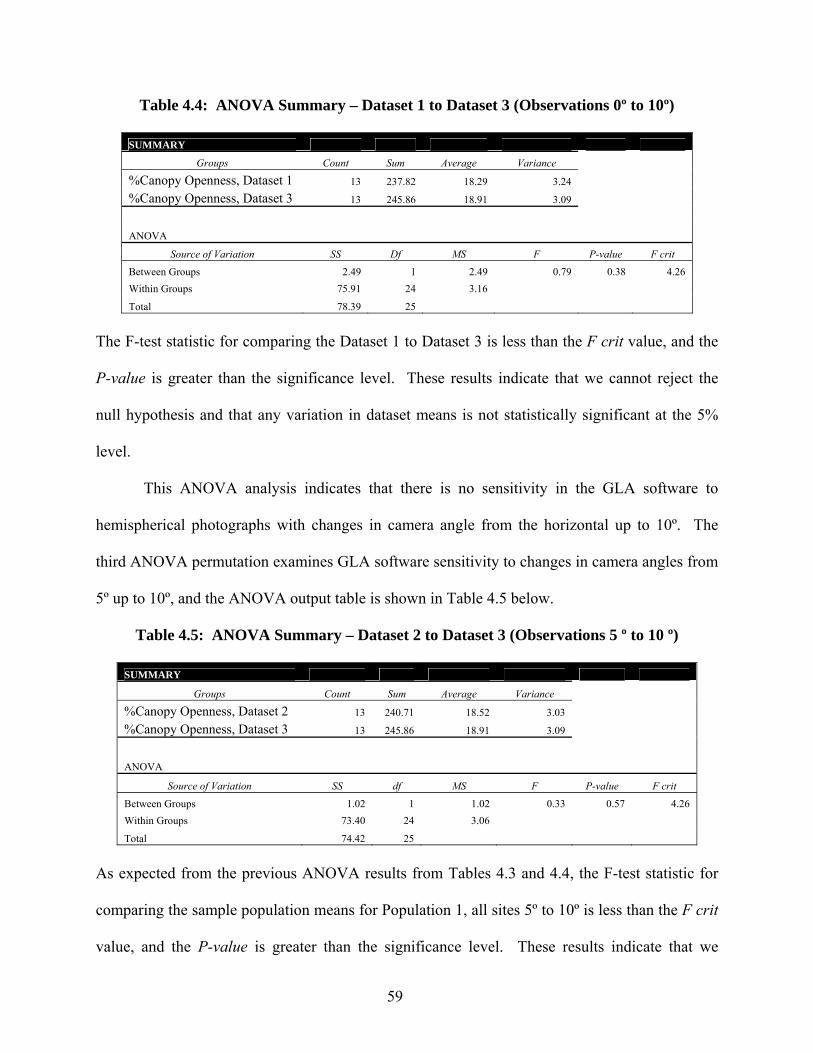
59

Table 4.4: ANOVA Summary – Dataset 1 to Dataset 3 (Observations 0º to 10º)

SUMMARY

Groups Count Sum Average Variance

%Canopy Openness, Dataset 1 13 237.82 18.29 3.24


ANOVA

Source of Variation SS Df MS F P-value F crit


Total 78.39 25

The F-test statistic for comparing the Dataset 1 to Dataset 3 is less than the F crit value, and the

P-value is greater than the significance level. These results indicate that we cannot reject the

null hypothesis and that any variation in dataset means is not statistically significant at the 5%

level.


hemispherical photographs with changes in camera angle from the horizontal up to 10º. The

third ANOVA permutation examines GLA software sensitivity to changes in camera angles from

5º up to 10º, and the ANOVA output table is shown in Table 4.5 below.

Table 4.5: ANOVA Summary – Dataset 2 to Dataset 3 (Observations 5 º to 10 º)

SUMMARY

Groups Count Sum Average Variance



ANOVA



Total 74.42 25

As expected from the previous ANOVA results from Tables 4.3 and 4.4, the F-test statistic for

comparing the sample population means for Population 1, all sites 5º to 10º is less than the F crit

value, and the P-value is greater than the significance level. These results indicate that we

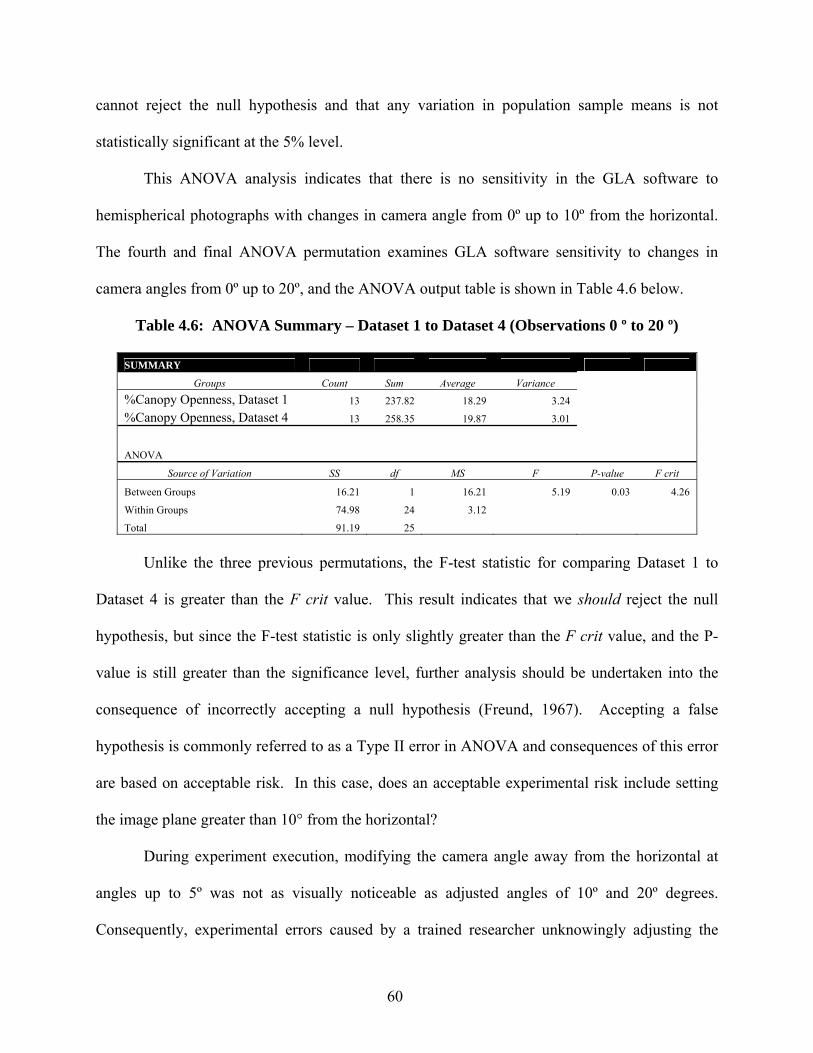
60

cannot reject the null hypothesis and that any variation in population sample means is not

statistically significant at the 5% level.


hemispherical photographs with changes in camera angle from 0º up to 10º from the horizontal.

The fourth and final ANOVA permutation examines GLA software sensitivity to changes in

camera angles from 0º up to 20º, and the ANOVA output table is shown in Table 4.6 below.

Table 4.6: ANOVA Summary – Dataset 1 to Dataset 4 (Observations 0 º to 20 º)

SUMMARY

Groups Count Sum Average Variance %Canopy Openness, Dataset 1 13 237.82 18.29 3.24 %Canopy Openness, Dataset 4 13 258.35 19.87 3.01

ANOVA


Between Groups 16.21 1 16.21 5.19 0.03 4.26

Within Groups 74.98 24 3.12

Total 91.19 25

Unlike the three previous permutations, the F-test statistic for comparing Dataset 1 to

Dataset 4 is greater than the F crit value. This result indicates that we should reject the null

hypothesis, but since the F-test statistic is only slightly greater than the F crit value, and the P-

value is still greater than the significance level, further analysis should be undertaken into the

consequence of incorrectly accepting a null hypothesis (Freund, 1967). Accepting a false

hypothesis is commonly referred to as a Type II error in ANOVA and consequences of this error

are based on acceptable risk. In this case, does an acceptable experimental risk include setting

the image plane greater than 10° from the horizontal?

During experiment execution, modifying the camera angle away from the horizontal at

angles up to 5º was not as visually noticeable as adjusted angles of 10º and 20º degrees.

Consequently, experimental errors caused by a trained researcher unknowingly adjusting the

61

camera to angles greater than 10º is considered unlikely. Therefore, we take the position that it is

an acceptable, albeit unlikely, experimental risk of setting the image plain to angles greater than

10° and up to 20° from the horizontal, and therefore cannot reject the null hypothesis and that

any variation in dataset means is not statistically significant at the 5% level.

4.6 Conclusion for Experimental Error ANOVA analysis of the four permutations was completed to test the sensitivity of GLA

software to camera angle modifications in computing the percentage of canopy openness values.

It was determined that camera angle modifications of 5° or even 10° do not greatly impact GLA

percentage of canopy openness results, thus resulting in us not rejecting the null hypothesis, HEx.

Angles greater than 10° can, however, slightly impact GLA software results, but any differences

in GLA values brought on by greater camera angles are considered an acceptable experimental

risk for the reasons listed above.

4.7 Processing Error

Two separate controlled processing errors were introduced during the processing of

hemispherical photographs by creating two new data populations (see Chapter 3 and Table 3.1),

which were both derived from the raw hemispherical photographs (Population 1). Population 2:

Modified Framed Image was completed to test the sensitivity of GLA software to brightness

values, and to see if the ground snow values were improperly categorized as sky values.

Population 3: Modified Threshold in GLA was completed to test for GLA software sensitivity to

modifications to its default threshold values. GLA software default threshold values were

modified from 128 to 100 for all hemispherical photographs to create Population 3.

ANOVA analysis was completed on all sites but only for the first observation (0°) in the

three populations, where the 0° observations from Population 1 were treated as Dataset 5, the 0°

62

observations from Population 2 referred to as Dataset 6, and Dataset 7 was composed of the 0°

observations from Population 3 (see Table 4.7). Only the 0° observations were used during

processing error analysis as the other observations related to introduction of experimental errors

(camera angling of 5°, 10° and 20° from the horizontal). ANOVA results and hypotheses tests

on the 0° observations will help determine the variability of these permutations within and

between populations, and the sensitivity of GLA software computations to processing errors.

Table 4.7: Variables used during Processing Error Analysis

Population Percent Canopy Openness Mean Values

Population Sample Used in Analysis

µ 5 Dataset 5 (0° Observations only) µ 6 Dataset 6 (0° Observations only) µ 7 Dataset 7 (0° Observations only)

The hypotheses tested through ANOVA analysis will determine if the mean values for the

different datasets shown in Table 4.7 are due to chance or reflect actual differences in dataset

means. The null hypothesis and alternative statements were described earlier in this chapter.

Quantitatively, the null hypothesis (HPr) and alternative (H1) statement are presented as:

HPr : µ 5 = µ 6 = µ 7

H1 : dataset means (µ) are not equal

Rejecting the null hypothesis indicates that the GLA software is sensitive to processing errors,

while not rejecting the null hypothesis indicates that the GLA software may account for

processing errors when completing its percentage of canopy openness computations.

ANOVA analysis was completed three times to assess if the GLA software was sensitive to

processing errors, such as interpretation of brightness values and modifications to threshold

values. The three ANOVA permutations include,

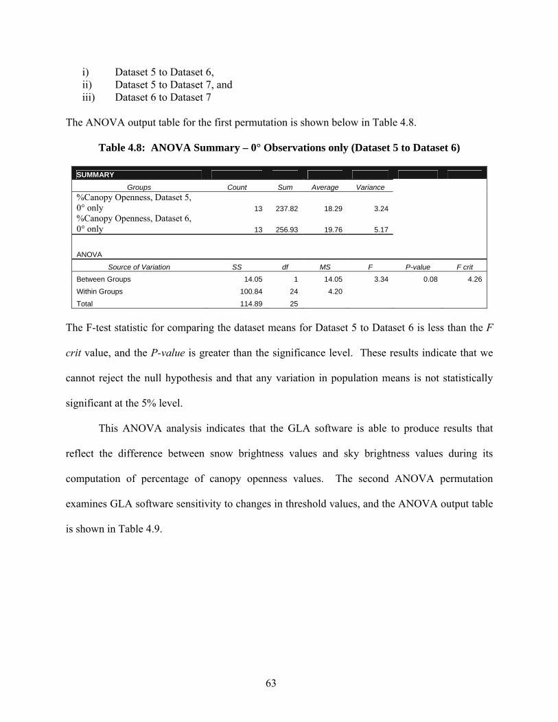
63

i) Dataset 5 to Dataset 6, ii) Dataset 5 to Dataset 7, and iii) Dataset 6 to Dataset 7

The ANOVA output table for the first permutation is shown below in Table 4.8.

Table 4.8: ANOVA Summary – 0° Observations only (Dataset 5 to Dataset 6)

SUMMARY Groups Count Sum Average Variance

%Canopy Openness, Dataset 5, 0° only 13 237.82 18.29 3.24 %Canopy Openness, Dataset 6, 0° only 13 256.93 19.76 5.17

ANOVA


Between Groups 14.05 1 14.05 3.34 0.08 4.26


Total 114.89 25

The F-test statistic for comparing the dataset means for Dataset 5 to Dataset 6 is less than the F

crit value, and the P-value is greater than the significance level. These results indicate that we

cannot reject the null hypothesis and that any variation in population means is not statistically

significant at the 5% level.

This ANOVA analysis indicates that the GLA software is able to produce results that

reflect the difference between snow brightness values and sky brightness values during its

computation of percentage of canopy openness values. The second ANOVA permutation

examines GLA software sensitivity to changes in threshold values, and the ANOVA output table

is shown in Table 4.9.

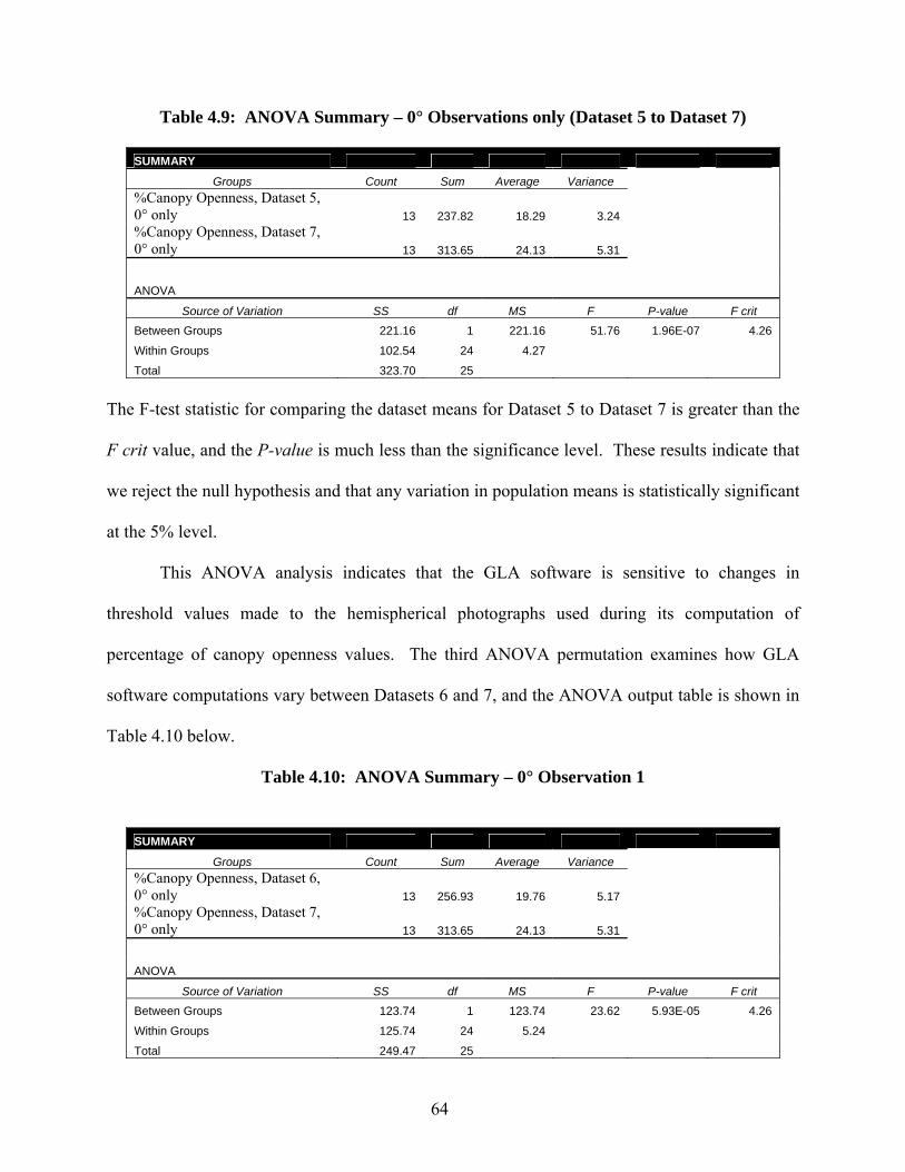
64

Table 4.9: ANOVA Summary – 0° Observations only (Dataset 5 to Dataset 7)

SUMMARY Groups Count Sum Average Variance

%Canopy Openness, Dataset 5, 0° only 13 237.82 18.29 3.24 %Canopy Openness, Dataset 7, 0° only 13 313.65 24.13 5.31

ANOVA


Between Groups 221.16 1 221.16 51.76 1.96E-07 4.26


Total 323.70 25

The F-test statistic for comparing the dataset means for Dataset 5 to Dataset 7 is greater than the

F crit value, and the P-value is much less than the significance level. These results indicate that

we reject the null hypothesis and that any variation in population means is statistically significant

at the 5% level.

This ANOVA analysis indicates that the GLA software is sensitive to changes in

threshold values made to the hemispherical photographs used during its computation of

percentage of canopy openness values. The third ANOVA permutation examines how GLA

software computations vary between Datasets 6 and 7, and the ANOVA output table is shown in

Table 4.10 below.

Table 4.10: ANOVA Summary – 0° Observation 1

SUMMARY

Groups Count Sum Average Variance %Canopy Openness, Dataset 6, 0° only 13 256.93 19.76 5.17 %Canopy Openness, Dataset 7, 0° only 13 313.65 24.13 5.31

ANOVA


Between Groups 123.74 1 123.74 23.62 5.93E-05 4.26


Total 249.47 25

65

The F-test statistic for comparing the dataset means for Dataset 6 to Dataset 7 is greater than the

F crit value, and the P-value is must less than the significance level. These results indicate that

we reject the null hypothesis and that any variation in population means is statistically significant

at the 5% level.

This ANOVA analysis, like the one in presented in Table 4.9, verifies that the GLA

software is sensitive to changes in threshold values made to the hemispherical photographs.

4.8 Conclusion for Processing Error The GLA software is capable of differentiating between snow and sky brightness values,

making it a useful tool in cryospheric research. The GLA software is, however, sensitive to

changes in the software parameters, such as modifications made to threshold values. It is then

suggested that these settings be left at default for use in mass collection and processing of

hemispherical photographs used in snow-based studies.

4.9 Conclusion Results using Population 2 (cropped hemispherical photographs) unintentionally provide

a means to address issues of compatibility of colour digital hemispherical photographs with the

GLA software. Colour aberration typically occurs along the outer fringe of the photograph, and

Population 2 had its outer fringe cropped off, thus providing a means to address and test this

potential systemic error. ANOVA results shown in Table 4.10 highlight the compatibility

between digital hemispherical photography and GLA software as the % Canopy Openness values

were not impacted by colour aberration, which was first mentioned by Frazer et al. (2001) in

Chapter 2.

66

CHAPTER FIVE: Summary and Conclusions

5.1 Introduction The Canadian Government’s responsibility to monitor its large Arctic region has put that

country at the forefront of both cryospheric research and remote sensing development (LeDrew

et al., 1995). Canada’s cryosphere environments are, however, degrading from climate change

and industrialization, thus threatening ecosystem diversity, altering physical features and

impacting some of the country’s industries, including farming.

One component of the cryosphere that has been negatively impacted by climate change is

seasonal snow cover. Canada’s snow accumulation has been increasingly variable and, as

evidenced by the 2001-2002 drought in south-central Canada, has greatly impacted Canada’s

Prairie Region. Snow cover’s SWE characteristic can be used to identify both snow

accumulation and depth. Many of Canada’s water-reliant industries monitor water levels, with

both snow accumulation and depth values being crucial to identifying spring runoff levels.

Spring runoff is of special concern in Canada’s Prairie region as runoff originating mainly from

the Rocky Mountains is needed to replenish water supply and reservoirs, in addition to ensuring

adequate soil moisture levels for the region’s farming industry.

Monitoring SWE is important to understanding the relationship between global climate

change and Canada’s variable snow accumulation, as well as helping to improve water

conservation and preparedness practices (Rango et al., 1983). Many organizations within

Canada recognize the importance of monitoring SWE and provide historical and current

cryospheric data, such as SWE, for use by the scientific and non-profit communities. These

organizations are summarized in Table 5.1.

67

Table 5.1: Current Organizations monitoring and providing information about Canada’s Cryosphere

Organization Purpose Approach Web Site

Canadian Cryospheric Information Network (CCIN)

Act as a cryospheric data and information portal among Canadian scientists and international colleagues

Provide central access to cryospheric information and data as provided to CCIN by the CRYSYS research council

www.ccin.ca

CRYosphere SYStem in Canada (CRYSYS)

Canadian-led project developing capabilities for monitoring and understanding issues of scale in cryospheric variables, in addition to further examining the role of the cryosphere in the climate system

Centralize project information and create a portal for education purposes containing basic definitions to pictures to overviews of different components of the cryosphere

www.crysys.ca

State Of the Canadian Cryosphere (SOCC)

Centrally provide historical and current information, as well as future state, of important cryospheric variables in Canada

Provide central location to easily access other cryospheric websites, including CCIN and CRYSYS, in addition to providing quick links to maps and graphs presenting historical and current states of the Canadian cryosphere

www.socc.ca

There are additional organizations that examine a portion of Canada’s cryosphere, but these

organizations focus on either a specific location, such as the Canadian Polar Commission

(www.polarcom.gc.ca), or cryosphere variable, such as the Canadian Ice Service (ice-

glaces.ec.gc.ca).

The CRYSYS website highlights one project that focuses on the use of remote sensing to

monitor SWE characteristics in Canada’s Prairie region. This project also supplies their

collected information to the public in easy-to-read generated maps through the SOCC initiative

68

(Environment Canada [socc.ca/SWE/snow_swe.html], 2008). This CRYSYS project is based

out of MSC’s Climate Research Branch, and its focus is the development of the passive

microwave SWE retrieval algorithm suite as led by Dr. Chris Derksen, and is the framework for

this thesis. The Climate Research Branch generated SWE maps series is, however, restricted to

Canada’s Prairie region.

Documentation accompanying the SWE maps indicates that as of 1999, a new SWE

algorithm has been used in generating the maps that takes into account forest vegetation in

computing its passive microwave-derived SWE values. The Climate Research Branch is still in

the process of developing its full algorithm suite so that its SWE estimates better and more fully

account for vegetation structure. This development includes refining its Prairie SWE algorithm

and eventually putting to operation its three remaining SWE retrieval algorithms.

The methodology developed in this study provides insight to the existing Prairie SWE

algorithm, and highlights the research of correction factors to account for vegetative structure,

which may aid in the development of the Boreal SWE retrieval algorithm. In this thesis we also

highlight the utility of a particular type of in situ remote sensing technique in monitoring and

assessing vegetative structure in a snow-covered boreal forest environment: hemispherical

photography. One means for accounting of vegetative structure in remotely sensed data is to

incorporate in situ data to act as ground-truthing when classifying the remotely sensed images.

The collection of in situ hemispherical photography was performed to test its effectiveness for

accounting for forest canopy structure through derived sky gap values (Zhang and Goodchild,

2002).

69

Chapters 3 and 4 highlighted that the in situ hemispherical photography can be collected

with relative ease, with the greatest concern being the logistics of remote location data collection

and computer processing of the images.

5.2 Major Findings The objective of this thesis was to examine and test the use of hemispherical photography

in obtaining sky gap estimates, with application to account for vegetation structure in ground-

truthing MSC’s boreal SWE algorithm. Manipulation of the conditions by which the

hemispherical photographs of the forest canopy were taken, including angle from horizontal,

cloud cover, and height above the ground, helped to determine the sensitivity and utility of sky

gap values derived from hemispherical photography. Conditions by which the resultant

hemispherical photographs were analyzed using the software highlighted any sensitivity to

changes in photograph or software settings. These conditions were introduced systematically

into the methodology and were referred to as experimental and processing errors.

ANOVA tests were used to evaluate the influence of experimental and processing errors

on the utility of hemispherical photographs to act as a tool for accounting of vegetative structure,

and to determine the variability of these permutations within and between populations and sites.

The hemispherical photographs were organized into three populations; raw data, modified frame

image and modified threshold values. The populations were further organized into datasets to

provide more sensitive error analysis, which reduced the potential for additional variability. All

hemispherical photographs had sky gap (% Canopy Openness) values derived using GLA

software, with ANOVA analysis performed on the resultant sky gap value. Major findings are

grouped into two categories, experimental error and processing error.

70

The first major finding of this study was that modifying the camera angle away from the

horizontal at measurements up to and including 10º do not greatly impact GLA software results.

Angles greater than 10° can, however, slightly impact GLA software results, but any differences

in sky gap values brought on by greater camera angles are considered an acceptable experimental

risk.

Camera angles of 0º, 5º, 10º and 20º were sampled for 13 different sites, and ANOVA

results on the raw images indicate that the 0º, 5º, and 10º population samples belong to a single

population. Only the raw image population was analyzed during experimental error analysis as

the two other populations relate to the introduction of processing errors. The 20º population

sample did initially suggest that they belong to a separate population, but with the F-test statistic

being only slightly greater than the F crit value, and the P-value being greater than the

significance level, it was determined to be a Type II error in ANOVA analysis, with the

consequences of this error based on acceptable risk. We take the position that it is an acceptable,

albeit unlikely, experimental risk of setting the image plain to angles greater than 10° and up to

20° from the horizontal.

Consequently, ANOVA results on the raw data for the different population samples

indicate that we cannot reject the null hypothesis, and that the population percent canopy

openness means values for the four population samples are equal, thus concluding that modifying

the camera angle up to and including 10º does not greatly impact GLA software results, with

camera angles up to 20º being an acceptable risk.

The second major finding of this study was that the Gap Light Analyzer (GLA) software

is capable of differentiating between snow and sky brightness values, making it a useful tool in

cryospheric research. The GLA software is, however, sensitive to changes in the software

71

parameters, such as modifications made to threshold values, used during its computation of

percentage of canopy openness values and it is suggested that these settings be left at their

default values.

ANOVA analysis was completed on all sites for the three populations, but for only the

first observation (0°). Only the 0° population sample was used during processing error analysis

as the 5°, 10° and 20° population samples related to the introduction of experimental errors.

ANOVA results on the raw, modified frame image, and modified threshold value datasets

indicate that we cannot reject the null hypothesis, and that the population percent canopy

openness means values for the three populations are equal, thus concluding that the GLA

software may account for processing errors.

The two major findings indicated that with minimal effort, hemispherical photography

may act as a correction factor to account for local scale land-cover variability with real-world

application including MSC’s boreal SWE retrieval algorithm. Thesis findings may also apply to

more traditional applications of hemispherical photography, such as characterizing light

environments for specific plants and leaf structures, which mainly apply to agricultural, forest

meteorologly and ecological applications (Chazdon and Field, 1987; Herbert, 1987).

Applications may include comparing sky gaps and leaf structures for varying climatic

conditions, including droughts (Becker and Smith, 1990). Chazdon and Field (1987) highlight

the utility of manual analysis of hemispherical photographs for spring to fall based ecological

studies, but also recognize that individual bias during manual analysis is a major limitation that

may be manual analysis with computerized processing. Thesis findings highlight that some

experimental and processing steps may be unnecessary when digitally analyzing hemispherical

photographs.

72

5.3 Sources of Error Sources of error in this study were mostly controlled, and categorized as either

experimental or processing errors, and were initiated as part of the methodology (see Chapter 3).

These errors were introduced to assess the sensitivity and utility of sky gap values derived from

hemispherical photography using GLA software. Additional sources of error included systemic

errors as evidenced by the problematic hemispherical photographs from the winter 2003 SWE

Scaling Experiment (see Figure 3.2). Consequently a second field experiment was held in

February 2004 to collect hemispherical photographs that had minimal systemic errors.

The February 2004 experiment provided the opportunity to prioritize the capturing of the

photographs, which provided for extra time in setting up the hemispherical photograph

experiment design (see Figure 3.8). Foreseeable systemic errors from the 2003 field experiment

that were addressed in the February 2004 experiment include having the base of the camera

platform consistently 1 metre from the earth’s surface; removing outside variables (such as

people’s heads); using a compass to ensure that north on each image was identified; using

consistent camera settings (either default or constant FOV); and using a level to measure the

camera’s angle from the horizontal.

There were, however, inconsistencies with the amount of cloud cover in the

hemispherical photograph’s FOV. Anderson (1964) suggests that all images be taken on cloudy

days. The images used in this study were a mixture of full sun, partial sun and cloudy.

Additionally, errors such as water droplets from snow on the camera lens rendered four

observations from one site defective, and were not included during ANOVA testing. It was also

noted that wind could be a factor in adding water droplets to the camera lens as snow would fall

from overhead branches during wind gusts.

73

It is then recommended that the photographs be taken on purely cloudy days with

minimal wind and where the temperature remains below 0°C, so as to reduce the concern for

water droplets on the camera lens, movement of the tree branches captured in the photograph,

and to maintain a constant amount of cloud coverage.

5.4 Future Research Demands Estimates of derived-SWE values from passive microwave remotely sensed data have

been improving with the introduction of correction factors to account for vegetative cover

(Environment Canada [socc.ca/SWE/snow_swe.html], 2008). These correction factors recognize

issues with using small scale remotely sensed data in a variable landscape. The SWE algorithm

suite correction factors take into account the vegetation covers effects on the remotely sensed

data, with the goal being to provide more representative SWE estimates. A SWE algorithm suite

that takes into account the geometry of vegetation would result in representative SWE estimates.

More accurate SWE values could be used to better prepare Canada’s agricultural community

about potential drought periods, as well as provide a more detailed view of how climate change

is impacting Canada’s climate and resultant environment.

It was determined that an easily designed experiment involving hemispherical

photography may act as a correction factor for accounting of vegetative structure when using in

situ remotely sensed data. This study also determined that hemispherical photography can be

applied to many other forestry uses, and although most research into the use of these types of

photographs are for mainly deciduous environments during the spring to fall seasons, there is

utility in this type of in situ remote sensing in cryosphere and coniferous-forest based studies.

74

APPENDIX 1.0

1.1 GLA© output data for Populations 1 through 3

Experiment Date: Thursday, February 19, 2004 Population #1 Population #2 Population #3

TIME TEMP. (ºC) WEATHER CONDITIONS SITE/DATA ID % CANOPY OPENNESS % CANOPY OPENNESS % CANOPY OPENNESS

10:54 AM A_0 19.47 21.38 25.67

10:55 A_5 20.31 22.45 27.26

10:55 A_10 22.04 23.99 30.25

10:56

-3

Overcast A_20 21.08 22.77 31.1

11:19 B_0 18.46 20.5 24.13

11:20 B_5 18.23 20.26 24.02

11:20 B_10 18.3 20.37 24.92

11:20

N/A

Overcast B_20 17.84 19.79 26.52

Note: large break because of equipment (thermometer) failure

1:33 PM C_0 16.8 18.03 23.14

1:33 C_5 16.72 18.03 22.94

1:34 C_10 16.88 17.81 22.82

1:34

N/A

Overcast C_20 19.1 19.03 25.32

1:51 D_0 15.6 17.08 22.36

1:52 D_5 15.44 16.94 21.82

1:52 D_10 15.67 17.2 22.38

1:52

0.5

Partly sunny wind increasing

D_20 17.07 17.89 24.5

2:19 E_0 17.13 18.95 23.82

2:20 E_5 17.01 18.46 23.33

2:20 E_10 17.31 18.88 24.32

2:20

-0.5

Partly sunny E_20 17.06 18.75 25.48

2:39 F_0 21.84 24.04 30.12

2:40 F_5 21.38 23.53 29.16

2:40 F_10 21.09 22.82 28.59

2:40

0

Partly sunny F_20 22.52 22.97 30.05

3:13 H_0 19.53 21.57 25.61

3:14 H_5 19.52 21.55 25.67

3:17 H_10 19.25 21.22 25.54

3:17

-1

Mainly sunny H_20 19.12 20.82 26.54

3:36 I_0 17.55 18.89 23.85

3:37 I_5 17.54 18.69 23.89

3:37 I_10 17.99 18.75 24.49

3:38

-1

Partly sunny I_20 20.51 21.06 28.46

75

GLA© output data for Populations 1 through 3 continued

Experiment Date: Thursday, February 19, 2004 Population #1 Population #2 Population #3

TIME TEMP. (ºC) WEATHER CONDITIONS SITE/DATA ID % CANOPY OPENNESS % CANOPY OPENNESS % CANOPY OPENNESS

4:00 J_0 18.12 18.55 23

4:00 J_5 18.53 19.19 23.88

4:00 J_10 19.55 20.77 26.11

4:01

-1

Partly sunny J_20 20.22 21.44 28.18

4:15 K_0 17.11 18.02 21.71

4:16 K_5 17.66 17.57 21.54

4:16 K_10 19.14 18.86 23.34

4:16

-2

Overcast K_20 20.66 20.99 26.54

4:35 L_0 21.29 23.7 26.01

4:36 L_5 21.18 23.56 26.04

4:36 L_10 20.79 23.12 25.85

4:36

-1

Partly sunny L_20 20.49 22.71 27.61

4:56 M_0 17.7 18.43 22.43

4:56 M_5 18.42 19.03 23.38

4:57 M_10 18.82 19.44 24.64

4:57

-2

Partly sunny M_20 20.71 21.52 28.68

5:15 N_0 17.22 17.79 21.8

5:15 N_5 18.77 18.43 22.58

5:15 N_10 19.03 18.79 22.82

5:16

-2

Partly sunny N_20 21.97 21.86 26.36

76

APPENDIX 2.0

2.1 Acronym List

Acronym Full Name

ANOVA ANalysis Of VAriance

FOV Field of View

GLA Gap Light Analyzer

GLI Gap Light Index

GORT Geometric-Optical Radiative-Transfer

LAI Leaf Area Index

MSC Meteorological Service of Canada

PAR Photosynthetically Active Radiation

PPFD Photosynthetic Photon Flux Density

SWE Snow Water Equivalent

UEBFC Utah Energy Balance Forest Canopy closure

2.2 Software List

Software Packages Uses

Excel, Microsoft Office Spreadsheet functions, i.e. sorting, ANOVA

Gap Light Analyzer, V 2.0 Sky gap analysis through calculation of % Canopy Openness values. Testing of processing errors through modification of threshold values.

Adobe Photoshop 7.0 Cropping hemispherical photographs to create Population 2 from raw data (Population 1)

77

REFERENCES

ACADEMIC REFERENCES Anderson,MC, 1964, Studies of the Woodland Light Climate: I. The Photographic Computation

of Light Conditions: The Journal of Ecology, v. 52, p. 27-41.

Barry,RG, R L Armstrong, A N Krenke, 1993, An Approach to Assessing Changes in Snow Cover: An Example for the Former Soviet Union, 25-33. Quebec City, Quebec, Proceedings of the 50th Eastern Snow Conference and 61st Western Snow Conference.

Barry,RG, J M Fallot, R L Armstrong, 1994, Accessing Decadal changes in the Cryosphere: Eurasian Snow Cover, 148-155. Nashville, Tennessee, Proceedings of the 5th Symposium on Global Change Studies, and the Symposium on Global Electrical Circuit, Global Change, and the Meteorological Applications of Lightning Information.

Barry,RG, J M Fallot, R L Armstrong, 1995, Twentieth-century variability in snow-cover conditions and approaches to detecting and monitoring changes: status and prospects: Progress in Physical Geography, v.19, p. 520-532.

Becker,P, A Smith, 1990, Spatial autocorrelation of solar radiation in a tropical moist forest understory: Agricultural and Forest Meteorology, v.2: 373-379.

Brown,RD, 1996, Evaluation of Methods for Climatological Reconstruction of Snow Depth and Snow Cover Duration at Canadian Meteorological Stations, 55-61, Williamsburg, Virginia, Proceedings of the 53rd Eastern Snow Conference.

Canham,CD, 1988, An Index For Understory Light Levels in and Around Canopy Gaps: Ecology, v. 69, p. 1634-1638.

Canham,CD, A C Finzi, S W Pacala, D H Burbank, 1994, Causes and Consequences of resource heterogeneity in forests: interspecific variation in light transmission by canopy trees: Canadian Journal of Forest Research, v. 24, p. 337-349.

Case,TJ, R N Fisher, 2001, Measuring and Predicting Species Presence: Coastal Sage Scrub Case Study, in CT Hunsaker, M F Goodchild, M A Friedl, T J Case (eds.), Spatial Uncertainty in Ecology: Implications for Remote Sensing and GIS Applications: New York, Springer, p. 47-71.

Chazdon,RL, C B Field, 1987, Photographic estimation of photosynthetically active radiation: evaluation of a computerized technique: Oecologia, v. 73: p. 525 – 532.

Chen,JM, T A Black, R S Adams, 1991, Evaluation of hemispherical photography for determining plant area index and geometry of a forest stand: Agricultural and Forest Meteorology, v. 56, p. 129-143.

Cihlar,J, 2000, Land cover mapping of large areas from satellites: status and research priorities: International Journal of Remote Sensing, v. 21, p. 1093-1114.

Culvenor,DS, 2003, Extracting Individual Tree Information: A Survey of Techniques for High Spatial Resolution, in M A Wulder, S E Franklin (eds.), Remote Sensing of Forest Environments: Concepts and Case Studies: Boston, Kluwer Academic Publishers, p. 255-277.

78

Curran,PJ, P M Atkinson, 1998, Geostatistics and remote sensing: Progress in Physical Geography, v. 22, p. 61-78.

Derksen,C, A Walker, E LeDrew, B Goodison, 2002, Time-series analysis of passive-microwave-derived central North American snow water equivalent imagery: Annals of Glaciology, v. 34, p. 1-7.

Derksen,C, R Brown, A Walker, B Brasnett, 2002a, Comparison of Model, Snow, Course and Passive Microwave Derived Snow Water Equivalent Data for Western North America. Stowe, Vermont, Proceedings of the 59th Eastern Snow Conference.

Derksen,C, E LeDrew, A Walker, B Goodison, 2000, Winter season variability in North American SWE distribution and atmospheric circulation: Hydrological Processes, v. 14, p. 3273-3290.

Derksen,C, 2002, Boreal Forest Snow Water Equivalent Scaling Experiment: Winter 2003 Field Experiment Science Plan. Downsview: Environment Canada, Climate Research Branch.

Engelbrecht,BMJ, H M Herz, 2001, Evaluation of different methods to estimate understorey light conditions in tropical forests: Journal of Tropical Ecology, v. 17, p. 207-221.

Englund,SR, J J O’Brien, D B Clark, 2000, Evaluation of digital and film hemispherical photography and spherical densiometry for measuring forest light environments: Canadian Journal of Forest Research, v. 30, p. 1999-2005.

Fournier,RA, R Landry, N M August, G Fedosejevs, R P Gauthier, 1996, Modelling light obstruction in three conifer forests using hemispherical photography and fine tree architecture: Agricultural and Forest Meteorology, v. 82, p. 47-72.

Fournier,RA, P M Rich, R Landry, 1997, Hierarchical characterization of canopy architecture for boreal forest: Journal of Geophysical Research, v. 102, p. 29445-29454.

Fournier,RA, D Mailly, J-M N Walter, K Soudani, 2003, Indirect Measurement of Forest Canopy Structure from In Situ Optical Sensors, in M A Wulder, S E Franklin (eds.), Remote Sensing of Forest Environments: Concepts and Case Studies: Boston, Kluwer Academic Publishers, p. 77-113.

Frazer,GW, CD Canham, KP Lertzman, 1999, Gap Light Analyzer (GLA), Version 2.0: Imaging software to extract canopy structure and gap light transmission indices from true-color fisheye photographs. Burnaby, B.C.: Simon Fraser University.

Frazer,GW, R A Fournier, J A Trofymow, R J Hall, 2001, A comparison of digital and film fisheye photography for analysis of forest canopy structure and gap light transmission: Agricultural and Forest Meteorology, v. 109, p. 249-263.

Frazer,G, 2007, Personal Communication.

Freund, John E. 1967. Modern Elementary Statistics. 3rd Ed. Englewood Cliffs, N. J.: Prentice-Hall, Inc.

Friedman,E, J Miller. 2003. Photonics Rule of Thumb: Optics, Electro-optics, Fiber Optics, and Lasers. 2nd Ed. New York: McGraw-Hill Professional.

79

Gendron,F, C Messier, P G Comeau, 1998, Comparison of various methods for estimating the mean growing season percent photosynthetic photon flux density in forests: Agricultural and Forest Meteorology, v. 92, p. 55-70.

Gong,P, B Xu, 2003, Remote Sensing of Forests Over Time: Change Types, Methods, and Opportunities, in M A Wulder, S E Franklin (eds.), Remote Sensing of Forest Environments: Concepts and Case Studies: Boston, Kluwer Academic Publishers, p. 301-333.

Hale,SE, C Edwards, 2002, Comparison of film and digital hemispherical photography across a wide range of canopy densities: Agricultural and Forest Meteorology, v. 112, p. 51-56.

Hardy,JP, R Melloh, G Koenig, D Marks, A Winstral, J W Pomeroy, T Link, 2004, Solar radiation transmission through conifer canopies: Agricultural and Forest Meteorology, v. 126, p. 257-270.

Hellstrom,R, 2000, Forest cover algorithms for estimating meteorological forcing in a numerical snow model: Hydrological Process, v. 14, p. 3239-3256.

Herbert,TJ, 1987, Area Projections of Fisheye Photographic Lenses: Agricultural and Forest Meteorology, v. 30, p. 215-223.

Houghton,JT, L Meira Filho, B Callander, N Harris, A Kattenberg, K Maskell (eds.), 1996, Climate change 1995: the science of climate change: Cambridge: Cambridge University Press.

Howard,JA, 1991, Remote Sensing of Forest Resources: Theory and application: London, Chapman and Hall, p. 298-350.

Inoue,A, K Yamamoto, N Mizoue, Y Kawahara, 2004a, Effects of image quality, size and camera type on forest light environment estimates using digital hemispherical photography: Agricultural and Forest Meteorology, v. 126, p. 89-97.

Inoue,A, K Yamamoto, N Mizoue, Y Kawahara, 2004b, Calibrating view angle and lens distortion of the Nikon fish-eye converter FC-E8: Journal of Forest Research, v. 9, p. 177-181.

Ishida,M, 2004, Automatic thresholding for digital hemispherical photography: Canadian Journal of Forest Research, v. 34, p. 2208-2216.

Kato,S, A Komiyama, 2002, Spatial and seasonal heterogeneity in understory light conditions caused by differential leaf flushing of deciduous overstory trees: Ecological Research, v. 17, p. 687-693.

LeDrew, Ellsworth F., Murray Strome, and Frank Hegyi, 1995, Introduction. In The Canadian Remote Sensing Contribution to Understanding Global Change. Ellsworth LeDrew, Murray Strome, and Frank Hegyi (eds.). Department of Geography Publication Series, No. 38, University of Waterloo: xxv – xxviii.

LeDrew, Ellsworth, 2002, A Uniquely Canadian Dimension to Climate Change: The Role of the Cryosphere in the Everyday Lives of Canadians. Faculty of Environmental Studies Research Lecture: Department of Geography, University of Waterloo.

80

Messier,C, P Puttonen, 1995, Spatial and temporal variation in the light environment by developing Scots pine stands: the basis for a quick and efficient method of characterizing light: Canadian Journal of Forest Research: v.25, p. 343-354.

Pomeroy,JW, D M Gray, N R Hedstrom, J R Janowicz, 2002, Physically Based Estimation of Seasonal Snow Accumulation in the Boreal Forest. Stowe, Vermont, Proceedings of the 59th Eastern Snow Conference.

Rango,A, J Martinec, J Foster, D Marks, 1983, Resolution in operation remote sensing of snow cover, 371-382. Proceedings of the Hamburg Symposium.

Rich,PM, 1990, Characterizing Plant Canopies with Hemispherical Photographs, in N S Goel, J M Norman (eds.), Remote Sensing Reviews: Instrumentation for studying vegetation canopies for remote sensing in optical and thermal infrared regions, v. 5, United Kingdom: Bell and Bain Ltd., p. 13-29.

Tarboton,D, C Luce, 1996, Utah energy balance snow accumulation and melt model (UEB), computer model technical descriptions and users guide. Utah Water Research Laboratory, Utah State University and USDA Forest Service, Intermountain Research Station.

Zhang,J, M F Goodchild, 2002, Chapter 4 Exploring Geographical Uncertainty, in J Zhang and M F Goodchild (eds.), Uncertainty in Geographical Information: New York, Taylor & Francis Inc, p. 69-92.

81

INTERNET REFERENCES Agriculture and Agri-Food Canada. “The 2002 Prairie Drought Summary – December 2002”

[Online] October, 2006. <http://www.agr.gc.ca/pfra/drought02sum_e.htm>

BERMS. “BERMS: Boreal Ecosystem Research and Monitoring Sites” [Online], February, 2007. <http://berms.ccrp.ec.gc.ca/e-main.htm>

CRYSYS. “Overview of CRYSYS Project and Recent Results, June 2002” [Online] February, 2007. <http://www.msc-smc.ec.gc.ca/crysys/overview/crysys_overview_2002_e.pdf>

Environment Canada. “Current State of the Cryosphere in Canada – Snow” [Online] February 2008. <http://www.socc.ca/SWE/snow_swe.html>

National Park Service. “GIS Responds to World Trade Center All-Risk Incident” [Online] April, 2008. <http://home.nps.gov/gis/applications/wtcgis.html>

Nikon. “Digital Camera Coolpix 950 Reference Manual” [Online] February, 2007. <http://oregonstate.edu/mediaservices/classup/manuals/cp950rm.pdf>

Sheffield Hallam University. “Beer’s Law” [Online] August, 2008. <http://teaching.shu.ac.uk/hwb/chemistry/tutorials/molspec/beers1.htm>

SOCC. “State of the Canadian Cryosphere” [Online] October, 2006. <http://www.socc.ca>

United Nations Environment Program. “Melting Permafrost may accelerate Global Warming, UNEP Scientists Warn” [Online] October, 2006. <http://www.unep.org/Documents.multilingual/Default.asp?DocumentID=102&ArticleID=2763>

World Glacier Monitoring Service. “Monitoring Strategy” [Online] April, 2008. <http://www.geo.unizh.ch/wgms/monitoring.html>.

Diane Redekop FINALTHESISS

Documents

Transcript of Diane Redekop FINALTHESISS