DIAGNOSIS AND PROGNOSIS OF ELECTRICAL AND

MECHANICAL FAULTS USING WIRELESS

SENSOR NETWORKS AND TWO-STAGE

NEURAL NETWORK CLASSIFIER

by

AKARSHA RAMANI

Presented to the Faculty of the Graduate School of

The University of Texas at Arlington in Partial Fulfillment

of the Requirements

for the Degree of

MASTER OF SCIENCE IN ELECTRICAL ENGINEERING

THE UNIVERSITY OF TEXAS AT ARLINGTON

August 2008

To my family.

ACKNOWLEDGEMENTS

I would like to acknowledge and extend my heartfelt gratitude to my su-

pervising professor, Dr. Frank Lewis, for his encouragement and motivation all

through my thesis; Dr. Wei-Jen Lee and Dr. Chiman Kwan for their timely inputs

and support, and Dr. Haiying Huang for agreeing to be on my defense committee.

I am grateful to Prasanna Ballal, my mentor at ARRI, for helping and guiding

me throughout my work. I would like to thank Matt Middleton and Chris Mc-

Murrough, without whom the thesis would not have reached its completion. I also

extend my gratitude to Aditya Telang, for his assistance with my documentation.

And most especially, I am thankful to my family for believing in my abilities and

encouraging me to strive for greater heights; I would have never reached here but

for their love and conviction.

Last but not the least, I express my gratitude to all my friends and colleagues at

ARRI and UTA, who have constantly motivated me to work at the best of my

potential.

This work has been sponsored by ARO grant DAAD 19-02-1-0366.

July 3, 2008

iii

ABSTRACT

DIAGNOSIS AND PROGNOSIS OF ELECTRICAL AND

MECHANICAL FAULTS USING WIRELESS

SENSOR NETWORKS AND TWO-STAGE

NEURAL NETWORK CLASSIFIER

AKARSHA RAMANI, M.S.

The University of Texas at Arlington, 2008

Supervising Professor: Frank L. Lewis

Diagnosis and isolation of electrical and mechanical problems in induction

motors has always been a very challenging task. Some of the common problems

in induction motors are: bearing, stator winding, and rotor bar failures. This the-

sis has three phases: The first one pertains to development of low-cost test-beds

for simulating bearing faults and short circuit stator winding faults in a motor.

Bearing fault is due to the failure of any of the components of the bearing and

the stator winding fault is due to the failure of insulation between the windings.

Bearing faults can be identified from the motor vibration signatures; where as

the stator winding fault can be identified through the measurement of the fault

voltage. Second, wireless modules for collection of voltage values and vibration

data from the test-beds have been developed. Wireless sensors have been used

because of their advantages over wired sensors in remote sensing and data col-

lection without human intervention. Finally, a novel two-stage neural network is

iv

used to classify various bearing and short circuit faults. The first stage neural

network estimates the principal components using the Generalized Hebbian Algo-

rithm (GHA). Principal Component Analysis is used to reduce the dimensionality

of the data and to extract the fault features. The second stage neural network

uses a supervised learning vector quantization network (SLVQ) utilizing a self or-

ganizing map approach. This stage is used to classify various fault modes. This

is followed by computation of performance metrics (Confusion Matrix, Receiver

Operating Characteristics and Health Index) in order to determine the condition

of the system at any instant of time and to predict the performance of the system

in future. Neural networks have been used because of their flexibility in terms of

online adaptive reformulation.

v

TABLE OF CONTENTS

ACKNOWLEDGEMENTS . . . . . . . . . . . . . . . . . . . . . . . . . . . iii

ABSTRACT . . . . . . . . . . . . . . . . . . . . . . . . . . . . . . . . . . . iv

LIST OF FIGURES . . . . . . . . . . . . . . . . . . . . . . . . . . . . . . . ix

CHAPTER PAGE

1. INTRODUCTION . . . . . . . . . . . . . . . . . . . . . . . . . . . . . . 1

1.1 Wireless Sensor Networks . . . . . . . . . . . . . . . . . . . . . . . 1

1.2 Condition Based Maintenance (CBM) . . . . . . . . . . . . . . . . . 2

1.3 Wireless Sensor Network for Condition Based Maintenance . . . . . 3

1.4 Related Work . . . . . . . . . . . . . . . . . . . . . . . . . . . . . . 4

1.4.1 Model Based Technique . . . . . . . . . . . . . . . . . . . . 5

1.4.2 Time-Domain Technique . . . . . . . . . . . . . . . . . . . . 6

1.4.3 Frequency Domain Technique . . . . . . . . . . . . . . . . . 6

1.4.4 Time-Frequency Domain Analysis . . . . . . . . . . . . . . . 7

1.4.5 Higher Order Spectral Analysis . . . . . . . . . . . . . . . . 9

1.4.6 Fuzzy Logic . . . . . . . . . . . . . . . . . . . . . . . . . . . 9

1.4.7 Neural Network (NN) Based Techniques . . . . . . . . . . . 10

1.5 Problem Definition . . . . . . . . . . . . . . . . . . . . . . . . . . . 11

2. EXPERIMENTAL SET UP OF THE TEST BEDS . . . . . . . . . . . . 14

2.1 Induction Motor . . . . . . . . . . . . . . . . . . . . . . . . . . . . . 14

2.1.1 Working Principle of AC Induction Working . . . . . . . . . 14

2.1.2 Construction . . . . . . . . . . . . . . . . . . . . . . . . . . 15

2.1.3 Internal Faults in an Induction Motor . . . . . . . . . . . . . 17

vi

2.2 Test Beds . . . . . . . . . . . . . . . . . . . . . . . . . . . . . . . . 20

2.2.1 Electrical Test Bed . . . . . . . . . . . . . . . . . . . . . . . 20

2.2.2 Mechanical Test Bed . . . . . . . . . . . . . . . . . . . . . . 26

2.3 Wireless Modules and Sensors . . . . . . . . . . . . . . . . . . . . . 29

2.3.1 Vibration Measurement . . . . . . . . . . . . . . . . . . . . 34

3. INTRODUCTION TO TIME DOMAIN ANALYSIS . . . . . . . . . . . 40

3.1 Time Domain Analysis . . . . . . . . . . . . . . . . . . . . . . . . . 40

3.1.1 Probability Density Function . . . . . . . . . . . . . . . . . 42

3.1.2 Root Mean Square and Peak Value . . . . . . . . . . . . . . 44

3.1.3 Statistical Parameters . . . . . . . . . . . . . . . . . . . . . 46

3.1.4 Covariance, Correlation and Convolution . . . . . . . . . . . 49

4. INTRODUCTION TO FREQUENCY DOMAIN ANALYSIS . . . . . . . 52

4.1 Frequency Domain Analysis . . . . . . . . . . . . . . . . . . . . . . 52

4.1.1 Properties of Discrete Fourier Transform . . . . . . . . . . . 56

4.1.2 Power Spectral Density . . . . . . . . . . . . . . . . . . . . . 57

5. TWO STAGE NEURAL NETWORK . . . . . . . . . . . . . . . . . . . . 60

5.1 First Stage Neural Network: Principal Components Estimation . . . 60

5.1.1 Convergence Rate . . . . . . . . . . . . . . . . . . . . . . . . 67

5.1.2 Extraction of the Principal Components . . . . . . . . . . . 68

5.1.3 Independent Component Analysis(ICA) . . . . . . . . . . . . 69

5.2 Second Stage Neural Network . . . . . . . . . . . . . . . . . . . . . 72

5.2.1 Self-Organizing Map(SOM) . . . . . . . . . . . . . . . . . . 74

5.2.2 Learning Vector Quantization(LVQ) . . . . . . . . . . . . . . 74

6. CLASSIFICATION OF FEATURE VECTORS . . . . . . . . . . . . . . 76

6.1 Classification . . . . . . . . . . . . . . . . . . . . . . . . . . . . . . 76

6.1.1 Different Techniques of Fault Classification . . . . . . . . . . 77

vii

7. EXPERIMENTAL RESULTS . . . . . . . . . . . . . . . . . . . . . . . . 97

7.1 Implementation . . . . . . . . . . . . . . . . . . . . . . . . . . . . . 97

7.2 Performance Analysis . . . . . . . . . . . . . . . . . . . . . . . . . . 97

7.2.1 Classification of the Input vectors . . . . . . . . . . . . . . . 97

7.2.2 Confusion Matrix . . . . . . . . . . . . . . . . . . . . . . . . 99

7.2.3 Health Index . . . . . . . . . . . . . . . . . . . . . . . . . . 103

8. CONCLUSION AND FUTURE WORK . . . . . . . . . . . . . . . . . . 107

REFERENCES . . . . . . . . . . . . . . . . . . . . . . . . . . . . . . . . . . 109

BIOGRAPHICAL STATEMENT . . . . . . . . . . . . . . . . . . . . . . . . 114

viii

LIST OF FIGURES

Figure Page

2.1 Parts of an Induction Motor . . . . . . . . . . . . . . . . . . . . . . 15

2.2 Cross Section of a Rolling Element Ball Bearing . . . . . . . . . . . 19

2.3 Conceptual Design of the test-bed for electrical faults . . . . . . . . 21

2.4 Experimental Set-Up for the Electrical Test-Bed . . . . . . . . . . . 22

2.5 Induction Coils Simulating the Fault Generator . . . . . . . . . . . . 23

2.6 Hall Effect Sensor . . . . . . . . . . . . . . . . . . . . . . . . . . . . 24

2.7 OPA-227 Pin Layout . . . . . . . . . . . . . . . . . . . . . . . . . . 25

2.8 Voltage Shifting Circuit using Op-Amp 227 . . . . . . . . . . . . . . 26

2.9 Conceptual design for the mechanical test-bed . . . . . . . . . . . . 27

2.10 Enclosed Setup for the experiment . . . . . . . . . . . . . . . . . . . 28

2.11 Metallic Disc with drilled holes . . . . . . . . . . . . . . . . . . . . . 29

2.12 Jennic Wireless Module . . . . . . . . . . . . . . . . . . . . . . . . . 33

2.13 PIC 18F4550 Module . . . . . . . . . . . . . . . . . . . . . . . . . . 34

2.14 Ultra Trak 750 Sensor . . . . . . . . . . . . . . . . . . . . . . . . . . 36

2.15 Accelerometer Sensing Node for recording 3D values . . . . . . . . . 37

2.16 Transceiver Unit of the Glink accelerometer . . . . . . . . . . . . . . 38

2.17 Diagram showing alignment of sensor with respect to the motor . . 39

3.1 Voltage values in the faultless condition . . . . . . . . . . . . . . . . 41

3.2 Voltage values in solid fault condition . . . . . . . . . . . . . . . . . 42

3.3 Voltage values in resistance fault condition . . . . . . . . . . . . . . 43

3.4 Probability Density Function of a faultless case . . . . . . . . . . . . 44

ix

3.5 Probability Density Function of a faulty case . . . . . . . . . . . . . 45

3.6 General Forms of Kurtosis . . . . . . . . . . . . . . . . . . . . . . . 47

3.7 Data Sample for finding Kurtosis values-Mechanical test bed . . . . 48

3.8 Data Sample for finding Kurtosis values-Electrical test bed . . . . . 49

3.9 Sensor/Data readings for computing the covariance values . . . . . . 50

3.10 Covariance Values . . . . . . . . . . . . . . . . . . . . . . . . . . . . 50

3.11 Correlation Values . . . . . . . . . . . . . . . . . . . . . . . . . . . . 51

3.12 Data to compute the correlation values . . . . . . . . . . . . . . . . 51

4.1 Frequency Spectrum for faultless condition-Electrical Test Bed . . . 53

4.2 Frequency Spectrum for a fault condition-Electrical Test Bed . . . . 54

4.3 Frequency Spectrum for faultless condition-Mechanical Test Bed . . 55

4.4 Frequency Spectrum for a fault condition-Mechanical Test Bed . . . 55

4.5 Frequency Spectrum of “20 g” weight in the outer ring . . . . . . . 56

4.6 Frequency Spectrum of “20 g” weight in the middle ring . . . . . . . 57

4.7 Frequency Spectrum of “20 g” weight in the inner ring . . . . . . . . 58

4.8 Frequency Spectrum of Solid Fault . . . . . . . . . . . . . . . . . . . 58

4.9 Frequency Spectrum of Resistance Fault . . . . . . . . . . . . . . . 59

4.10 PSD of a 20mH inductance added to the middle of the coil . . . . . 59

5.1 PCA Neural Network Model for Principal Component Extraction . . 66

5.2 Data Points Tracking a person on the Ferris Wheel . . . . . . . . . 72

5.3 LVQ Network . . . . . . . . . . . . . . . . . . . . . . . . . . . . . . 73

6.1 Some Basis Functions in Wavelet Analysis . . . . . . . . . . . . . . 78

6.2 Wavelet Transform . . . . . . . . . . . . . . . . . . . . . . . . . . . 80

6.3 Linguistic Variables denoting Induction motor Stator condition . . . 83

6.4 Fuzzy membership function for the stator currents . . . . . . . . . . 84

6.5 Fuzzy membership function for the stator condition . . . . . . . . . 85

x

6.6 Three state left-to-right Hidden Markov Model . . . . . . . . . . . . 86

6.7 Multiplayer Neural Network Architecture with two hidden layers . . 89

6.8 A Neuron Model . . . . . . . . . . . . . . . . . . . . . . . . . . . . . 90

7.1 Classified Output-Mechanical Test Bed . . . . . . . . . . . . . . . . 98

7.2 Classified Output-Electrical Test Bed . . . . . . . . . . . . . . . . . 99

7.3 Confusion Matrix . . . . . . . . . . . . . . . . . . . . . . . . . . . . 100

7.4 Confusion Matrix of testing data for the Mechanical Test Bed . . . . 101

7.5 Receiver Operating Characteristics of the Mechanical Test Bed . . . 102

7.6 Receiver Operating Characteristics of the Electrical Test Bed . . . . 103

7.7 Health Index for the Mechanical Test Bed . . . . . . . . . . . . . . . 105

7.8 Health Index for the Electrical Test Bed . . . . . . . . . . . . . . . . 106

xi

CHAPTER 1

INTRODUCTION

Failure avoidance is one of the main approaches for ensuring the quality and

performance of a system. There are two main types of failure avoidance in terms

of maintenance, namely preventive and corrective. In preventive maintenance, the

focus is on keeping the equipments in good operating condition, in order for it to

indicate the possible occurrence of a failure, so that actions can be taken to avert

the failures [1]. In corrective maintenance, a repair is performed after a failure

has occurred. Condition-based maintenance (CBM) is an approach of preventive

maintenance. The process of CBM involves monitoring the system, predicting

failures and making repairs before these failures occur. A system can contain

many fault modes and a decision has to be taken on the type of repair necessary

for eliminating any future faults.

1.1 Wireless Sensor Networks

Monitoring of the system is done using a range of sensors which can ei-

ther be wired or wireless. Wireless sensors are generally used to enable remote

monitoring. Wireless Sensor Networks (WSN) provide an intelligent platform to

gather and analyze data without human intervention [1]. Typically, a sensor net-

work consists of autonomous wireless sensing nodes that are organized to form a

network. Each node is equipped with sensors, embedded processing unit, short-

range radio communication module, and power supply, which is typically 9-volt

battery. With recent innovations in MEMS sensor technology, WSN hold signif-

1

2

icant promise in many application domains.Description of the parts of a wireless

sensor is as follows [2]:

• Sensing Unit:Consists of a sensor and an Analog to Digital Converter (ADC).

The analog signals from the sensor which could be light, vibration or tem-

perature depending on the application of the sensor is converted to digital

values using the ADC.

• Processing Unit:Acts upon the signal sent from the sensing unit.

• Transreceiver Unit:Connects the sensor nodes to the network.

• Power Unit: For small fields, replaceable batteries are used where as recharge-

able batteries are used for remote locations.

Additional units such as localization module, mobilizer unit and a power generator

can be used depending upon the application. The localization module helps in

finding the location of the senor node in the field [2]. The mobilizer unit connects

the sensors to the mobile robots.

1.2 Condition Based Maintenance (CBM)

Condition Based Maintenance is an automatic process which determines

the occurrence of a fault in the system and subsequently diagnoses the cause of

it. It makes use of sensors, algorithms, models and automated reasoning for the

monitoring and maintenance task. One of the biggest advantages of Condition

Based Maintenance is reduction of life-cycle costs by efficient planning and effec-

tive maintenance, which in turn is brought about by understanding of the working

of the equipments and the machineries. Assessing the health of machinery helps

in increasing the productivity and reliability of the machine as the faults can be

diagnosed and corrected on time before it takes a bigger dimension. Prior warn-

ing of an impending failure maximizes effectiveness of the maintenance repair and

3

minimizes downtime and resource requirement. CBM technology also provides

significant savings compared to preventive maintenance based systems on run-to-

fail-maintenance [3]. In order for a condition based maintenance system to be

effective, it should operate as a system which detects and classifies the incipient

faults, predicts the remaining life cycle of the equipment, supports the operator’s

decision for the course of action; interfaces with the control system to take ac-

tion; aids the maintainer in making repairs; and provides feedback to the logistics

support and machinery design communities [3].

1.3 Wireless Sensor Network for Condition Based Maintenance

Real time data interpretation which is one of the primary ingredients of CBM

are systems which mature with time. Distributed date acquisition which is another

important aspect of CBM, should hence be appropriate for both maintenance

and monitoring systems. Details on this can be obtained from [1]. Wireless

Sensors help in providing a component in controlling the machinery as well as

for identifying the system. Wireless Sensors have an edge over the conventional

wired systems in terms of being installed in hazardous, restricted and difficult to

reach areas.

The WSN help in collecting data from the various distributed sensors such as

accelerometer, temperature sensors, light sensors etc. which could then be used for

diagnostic and prognostic purposes. The results obtained through the running of

these data are compared with the stored fault pattern library in order to diagnose

faults and eventually upgrade the existing fault pattern library. The final step

involves estimating the Remaining Useful Life of the equipment which would be

useful to the maintenance personnel.

4

1.4 Related Work

Diagnosis and isolation of electrical and mechanical problems in induction

motors has always been a very challenging task. Some of the common problems in

induction motors are: bearing problems, followed by stator winding failures and

rotor bar failures, out of which bearing faults account for 40% of all the failures.

Since the bearings carry the weight of the rotor, its fault diagnosis becomes very

important [4]. Vibration monitoring is one of the methods used for bearing fault

analysis. Vibration monitoring for the critical power plant components has been

used for a number of years. There are several things that need to be kept in

mind for online health monitoring systems [5]. Signals that can help in diagnosis

and prognosis must be identified through the right type of sensors and supporting

instrumentation. Basic signal processing techniques which can highlight the fault

signature and suppress the dominant system dynamics and noise must be taken

into consideration. The final step should be the development of detection and

decision making process for prognosis. There are many challenges that need to be

faced before successful implementation of diagnosis and prognosis, for example,

for an induction motor the magnetic flux distribution is the best indicator for the

stator winding fault, but this requires a good magnetic sensor to be fixed inside

the motor, which could prove to be expensive and a difficult task. Therefore, a

solution for this could lie in measuring the fault current, which should be analyzed

properly for detection and decision making, but there are certain problems such

as: a) The fault signature, i.e., the stator current is 50 − 80dB smaller than

the signals themselves [5].In such cases, even the manufacturing defects could be

treated as fault signals. b) The other problem faced is due to the fact that no two

machines have identical characteristics, even if they are from the same assembly

5

line. Therefore, systems need to be developed which can overcome these problems.

There are two ways in ways in which the bearing maintenance can be done:

1. By estimating the bearing life based on statistical methods. But this is not a

very appropriate method as there could be post manufacturing defects that

might give a wrong estimated life span based on the statistical analysis of

experimental data. Their inaccuracy also lies in the fact that they do not

work real time to give the results. Therefore, we go for the second method.

2. Bearing condition monitoring and diagnosis, where signal processing tech-

niques can be used for real time monitoring. This is generally done using

two types of information - vibration and acoustics and secondly, current and

electromagnetic flux information.

Some of the fault diagnosis techniques which have been proposed have been dis-

cussed in the following section.

1.4.1 Model Based Technique

In Model Based technique, a mathematical model is tried to fit into a me-

chanical system. They match the vibration response of the system due to the

faults present in the bearing [6]. These models are system dependent and require

true knowledge of the system being modeled [6]. In the technique proposed in [7],

the description of the vibration produced by a single point defect on the inner race

of a rolling element bearing under constant radial load was done with the help of a

model. The bearing geometry, shaft speed, bearing load distribution were some of

the features incorporated by the model suggested. The model helped in comparing

the predicted and demodulated vibration spectra.

6

1.4.2 Time-Domain Technique

Time Domain analysis is one of the simplest methods for detecting incipient

bearing faults. It can be done either visually or by applying some statistical

parameters such as Crest factor, Root Mean Square Value, Kurtosis Value etc.

These have a greater value when the machine is under fault compared to the

faultless condition. Parameters like crest factor and kurtosis give spikiness of

the signal and not the vibration magnitude. Initially, the crest factor and kurtosis

increase as the spikiness of the vibration increases, but as the damage increases the

vibration becomes random and these values move towards normal values. Thus,

the time domain analysis lacks the ability to track the defects in the later stages

of the fault. Time domain analysis technique to detect the bearing faults was

used in [8] and [9]. The skew values of rectified data and the kurtosis values of

the unrectified data were used to detect the bearing fault. These results were

independent of load and speed variations. In [9] statistical parameters (Crest

Factor and Skew) were used to detect vibration and sound pressure signals to

detect the bearing defects. Even beta distribution function was used in the same

paper but it was inferred they did not prove to be very helpful in identifying

different types of bearing defects.

1.4.3 Frequency Domain Technique

In Frequency Domain Analysis frequency components and their amplitudes

are used for detecting bearing faults. The FFT of signal is analyzed, which shows

peaks and harmonics in the vibration spectra at the bearing defect frequency in

the event of a fault. These peaks show a marked increase as the severity of the

fault increases. When there are a large number of frequency components in the

spectrum and the signal to noise ratio is low, it becomes difficult to distinguish

7

between the faults and the noise components. This therefore, becomes a drawback.

Envelope Analysis, also known as High Frequency Resonance Technique has been

used to overcome this problem which has been studied in [10]. It is based on

the concept that every time the raceway is hit by a localized defect, an impulsive

force gets generated exciting the resonance of the mechanical system between the

point of impact and the point of measurement. This method helps in getting the

amplitude modulation of the resonance which lets the location and detection of

the defect to be known.

1.4.4 Time-Frequency Domain Analysis

Time-Frequency Domain Analysis uses both time and frequency domain in-

formation to detect the transient features such as impact. There are a number

of time-frequency domain techniques such as Short Time Frequency Transform

(STFT), the Wigner-Ville Distribution (WVD) and the Wavelet Transform (WT).

In cases where the signal to noise ratio is low and there is a presence of a lot of

frequency components, these time-frequency domain techniques prove to be useful

in detection of faults as explained in [11].

In [5], a solution for bearing outer race failure and faults due to stator voltage

imbalances have been suggested, where the concept of machine modeling along

with wavelet and symbolic dynamic analysis has been used for early detection of

faults in an induction motor. Development of sensor fusion technique gives a prob-

abilistic approach to these problems in induction motors. The method extends the

D-Markov process to combine the information from both electrical and mechanical

sensors. The vibration data that is obtained is analyzed using Continuous Wavelet

Transform which has been discussed in detail in Chapter 6. Parks vector modulus

has been computed on the signals that have been obtained from the machine un-

8

der consideration, which converts the instantaneous 3-phase stator current (R3)

signals into orthogonal reference frame (R2) and then again this value is converted

to a single value (R) using a modulus operator. The time domain signals that are

obtained from the above method is analyzed using wavelet transform. This is then

followed by Markov machine construction, which lets compression of information

and helps is giving an accurate measure of the fault. This measurement of fault

leads to an estimate of the health of the machine.

There may be certain disadvantages of using CWT in analysis: 1) there is a prob-

lem of redundancy associated with CWT - the calculation of the wavelet transform

is done by continuously shifting a continuously scalable function over a signal and

calculating the correlation between the two. These scaled functions do not give an

orthogonal basis function and hence, result in redundancy. This may sometimes

not be looked as a great disadvantage because making a signal orthogonal, reduces

the Signal to Noise Ratio. 2)There are an infinite number of wavelets present in

the wavelet transform which have to be reduced to a smaller amount for further

analysis. 3) For most of the wavelet transform, analysis can be done only mathe-

matically and hence it poses a limitation. This makes it necessary to use Discrete

Wavelet Transform. But the use of DWT for analysis makes the signal no longer

shift-invariant, which means that the time shifted version and the wavelet trans-

form of the same signal are not shifted versions of each other.

In [12], Multi-Resolution Analysis using wavelet technique has been used to iden-

tify thermal degradation or degradation via electrical charge of the bearing, where

an increase in the characteristic frequencies can be captured when the bearing

undergoes degradation. The MRA calculates the general RMS trend for the mea-

sured vibration signals from the bearings. The higher frequencies dominate the

signal when the motor becomes old and hence, gives an indication of bearing

9

damage. The MRA therefore, gives the bearing information without distorting

the original signal. Hence, this paper proposed a method to find the age of the

three phase squirrel cage motor through analysis of the vibration spectra from the

bearings.

In [13], wavelet transform based bearing-localized defect detection has been pre-

sented, where, wavelets are applied to detect the periodic structural ringing due

to repetitive impulsive forces created when rolling element passes over a defect.

This proposed a method which reduced the compromise on frequency resolution

for time localization.

1.4.5 Higher Order Spectral Analysis

Higher Order Spectral Analysis which describes the degree of correlation

among different frequencies present in the signal can also be used for fault detec-

tion. When there are large values of phase correlation among the harmonics of

defect frequency, it indicates some bearing fault. Bicoherence has been used for

analysis in the research work [14] which helps in extraction of the features deter-

mining the condition of the bearing. Bicoherence has been used to find the degree

of phase correlation among any three harmonics of the bearing characteristic defect

frequencies.

1.4.6 Fuzzy Logic

Diagnosis of the frequency spectra of the bearing fault can also be done with

the help of fuzzy logic if the input is processed in the right way as mentioned in

the work presented in [15]

10

1.4.7 Neural Network (NN) Based Techniques

Neural Network Approach makes use of pattern identification technique to

detect the bearing faults. Vibration monitoring using neural networks has been

done in [16] [17]. The extracted features from the vibration signals are used for

training the network, which in turn is used to match the condition of the bearing.

Analysis using Artificial Neural Network (ANN) is very useful when a large amount

of data needs to be classified. Data classification (pass or fail) using ANN helps

in letting the user know whether the data can be used for further analysis. Since

it does not require development of decision rules, its more adaptable to decision

rules[18]. Some of the advantages of using ANN are:

1. The weights used in ANN make it more robust compared to the Decision

trees.

2. The performance of ANN is improved through learning, which continues

even after the application of training set.

3. The error rate is low and the accuracy is high after the training.

4. They are more robust in noisy environments.

Some of the applications of ANN are:

• Statistical Modeling

• Image Compression

• Optical Character Recognition

• Medical diagnosis based on some symptoms

• Industrial Adaptive Control

In the analysis proposed in [19], a multi-layered feed forward NN trained

with Error Back propagation technique and an unsupervised Adaptive Resonance

Theory-2 (ART2) based NN was used for detection and diagnosis of localized faults

in ball bearings. The NN was trained using the statistical parameters obtained

11

from the signals under faultless and fault condition. The state of the ball bearing

was obtained from the output of the Neural Network.

In this thesis, we have made use of a two stage Neural Network through which

online adaptive reformulation is possible. This method eliminates the need for the

entire set of data to be present for classification as opposed to back propagation

method and hence, saves on the processing time if the volume of data is large.

Principal Component Analysis for feature extraction used in the first stage of NN

is advantageous compared to statistical methods as it avoids batch processing.

The proposed algorithm works well both with linear and non-linear systems in

comparison to Radial Basis Function and back propagation methods, which work

best when the system is linear. The analysis used in this work is more accurate

compared to time domain and frequency domain techniques.

1.5 Problem Definition

The work in this thesis puts forward a method for machine maintenance

and monitoring through signal processing techniques by measuring the vibration

and fault current. A wireless sensor network with advanced prognostic capability

for monitoring critical power plant components has been proposed. The proposed

system combines the hardware and the prognostic software in a unified frame-

work which will subsequently reduce the system downtime and the maintenance

cost. The data collection part consists of the test-beds (for generation of fault

signals) and wireless sensors and modules (for recording the fault information),

and a Personal Computer (for storing the fault values for analysis). The analysis

involves using Artificial Neural Network based approach which would help in iden-

tifying the degraded state of the system or more precisely, it helps in determining

the point at which the degradation has begun. ANN has been used because of

12

its good functional approximation property and extraordinary ability on pattern

recognition.

The advantages of the proposed system are:

• Saving in installation cost The proposed WSN system can be set up in

a short time of around 1 hour and has a low installation cost. This is much

lesser compared to cost of wired network which ranges from 10−1000 per

foot. The buffer and the sampling rate of these sensors can be kept high.

• Continuous and Real Time Collection of Data Since the sensing is

continuous and real time, the failures can be detected at an early stage

itself. Hence, it is helpful in preventive maintenance.

• Low Cost The sensors which have been used in the experiment are inex-

pensive. Hence, their usage saves on the cost.

• Portable hardware processor with state-of-the-art prognostic algo-

rithm The data can be measured on a continuous basis with the help of the

sensors. Even a Data Acquisition Card can be used to record the data on a

continuous basis on a PC.

• Use of Advanced Prognostic Tools Prognostic tools like ANN, and Hid-

den Markov Model can be used for prognosis for Condition Based Mainte-

nance.

• Performance of the Algorithm used The performances of these prognos-

tic algorithms used have been proved through various researches that have

taken place in the similar field.

The work also proposes a novel two-stage neural network to classify var-

ious short circuit and bearing faults. The first stage neural network estimates

the principal components using the Generalized Hebbian Algorithm (GHA). Prin-

cipal Component Analysis is used to reduce the dimensionality of the data and

13

to extract the fault features. This gives the flexibility of updating the principal

components online as new data comes in. The second stage neural network uses a

supervised learning vector quantization network (SLVQ) utilizing a self organizing

map approach. This stage is used to classify various fault modes. Neural networks

have been used because of their flexibility in terms of online adaptive reformula-

tion. In the end, a discussion on the performance of the proposed classification

method has been done.

The preceding section 1.4 gave an insight into the various researches that

have gone in the field with a brief introduction to the work that is going to be

explained in the forthcoming chapters. The second chapter explains in detail the

experimental set up for the the mechanical and electrical test beds, the wireless

modules and sensors used in these test beds for measuring the signals. The third

chapter provides information regarding the various time domain techniques and

their application to the signals that have been recorded for the experiment. The

fourth chapter describes the various frequency domain techniques and the manner

in which they have been used for the data obtained from the two test beds. Fifth

chapter gives in detail the Principal Component Analysis and the two stage neural

network used in this thesis. Sixth chapter describes the various classification

techniques. The results are presented in the seventh chapter followed by conclusion

and future work in the eighth chapter.

CHAPTER 2

EXPERIMENTAL SET UP OF THE TEST BEDS

One of the prime focus of this thesis is development of test beds for recording

signals from the machines for “Condition Based Maintenance”. Therefore, this

along with the appropriate selection of sensors for the experimentation forms an

important part. This chapter is broadly divided into three sections and hence,

explains: a) Induction Motor- its working principle, parts and types of internal

faults in it. b) The detailed description of experimental set-up of the two test beds

- electrical and mechanical, and c) The wireless modules and sensors used in the

experiment.

2.1 Induction Motor

The Induction Motor is a type of AC motor where, power is supplied to

the rotor by means of electromagnetic induction. Because of the relative motion

between the rotor circuits and the rotating magnetic field produced by the stator

windings, a torque is produced which causes the rotation. The following sections

give an insight into the operation and the fault types in Induction Motors.

2.1.1 Working Principle of AC Induction Working

The AC induction motor is a rotating electric machine which operates from

a three phase alternating voltage source. The induction motors are so called

because the current in the rotor conductors are supplied by induction. The three

phase stator has three windings which are displaced by 120◦. When currents flow

14

15

through the three symmetrically placed windings, a sinusoidally distributed air

gap flux generating the rotor current is produced. The rotor conductors are cut

by the alternating field in the stator set up by the alternating supply, thereby

inducing alternating current in the armature conductors. The interaction of this

sinusoidally distributed air gap flux and induced rotor currents produces a torque

on the rotor to give the mechanical output. The electromechanical interaction

between the stator and the rotor also constitutes transformer action. More details

can be found in [5]

2.1.2 Construction

Figure 2.1 [12] shows the parts of an Induction motor.

Figure 2.1 Parts of an Induction Motor

16

The two main parts of the induction motor are:

• Stator

• Rotor

The stator consists of a core of stacked, insulated, iron laminations with Polyphase

windings of insulated copper wire filling the slots in the core. The windings of

the stator are such that they produce an air gap magnetic motive force which is

symmetrically distributed around the magnetic poles. The rotor also consists of a

core of stacked, insulated, iron laminates. The slots are filled by aluminum bars

or copper windings. There are two types of rotors:

• Squirrel Cage Rotor

• Slip-Ring Rotor

Squirrel Cage Induction Motor

The name comes because of its shape: a cylindrical cage comprised of axial bars

terminated in annular rings. Cast Aluminum is used for the bars and the end rings.

The conductors are generally skewed along the rotor length to reduce the noise

and torque fluctuations. The thin laminations reduce the eddy current losses.

Slip-Ring Induction Motor

In this case the rotor windings are made up of wire and have the same number of

poles as the stator winding. Electrical connections are made from the rotor to the

ring. Brushes which are in contact with the rings transfer electric power to the

exterior part such as variable resistor which can help changing motor’s slip rate.

These require more maintenance and are more expensive compared to squirrel

cage induction motor.

17

2.1.3 Internal Faults in an Induction Motor

The faults in induction motor can be categorized as electrical or mechanical

faults. Electrical faults can be further sub-divided into stator or rotor faults. The

mechanical faults are the faults associated with the bearings of the machine [5].

2.1.3.1 Stator Faults

The stator faults pertain to the short circuit or open circuit of the stator

windings. Short circuit of the windings are caused due to

• failure of the winding insulation between turns within a phase coil

• failure of the winding insulation between turns of different phases

• failure of insulation between a turn and the stator core

The failure of insulation may be because of thermal, mechanical, chemical or

environmental stress.

• Thermal stresses are caused due to: overloading, unbalanced phase voltages,

obstructed ventilation and high ambient temperature.

• Electrical stresses are due to excessive voltages which are caused due to:

switching induced over voltages, lightening and variable frequency drives.

This would eventually lead to the breakdown of the dielectric.

• Mechanical stresses develop due to the relative motion between the coil bun-

dles and the stator, leading to loss of insulation. It can also be developed

due to relative motion of the conductors arising from vibration or magnetic

forces.

• Environmental stresses are caused due to moisture, chemicals and foreign

particles present in the atmosphere.

18

2.1.3.2 Rotor Cage Faults

The rotor is subjected to much lower voltages and much higher temperature

compared to the stator windings. Therefore, the most common failure mode in

rotors is open or broken rotor bar. This in turn can be caused due to mechanical,

thermal or residual stresses. Much of the thermal stresses in rotor are due to it

design and construction. The mechanical causes are magnetic forces, vibrations

and shock which is much greater than what the stator is subjected to. The rotor

gets affected by only those stresses which affect its geometry. These stresses can

be present in any of the planes-tangential, radial or axial. Whenever there is

a transition from no load to loaded condition, the stresses produced result in a

change in the rotor geometry and hence, produce vibrations.

2.1.3.3 Bearing Faults

Bearing faults are the most common faults occurring in all the machines

probably because of the reason that they carry the weight of the rotor. Rolling

bearings generally consist of two concentric rings (called the outer raceway and

inner raceway, respectively) with a set of rolling elements running in their tracks.

The rolling elements come in the following standard shapes: the ball, cylindrical

roller, tapered roller, needle roller, and symmetrical and unsymmetrical barrel

roller [5]. In order to have uniform spacing and for prevention of mutual contact,

the rolling elements in a bearing are guided in a cage. The rolling element type

is the most common bearing type which can be seen in the figure 2.2 [5]. Each

component of the bearing can undergo a failure in order to cause the fault. Some

of the causes of this fault are:

19

Figure 2.2 Cross Section of a Rolling Element Ball Bearing

• Mechanical Damage: Improper handling of the bearings results in dents

and nicks, causing displacement of the metal particles which can intro-

duce secondary effects in the motor when they indent the raceway. Even

brinelling (permanent indentation due to overload) might occur due to im-

proper mounting techniques.

• Damage due to wear: The wear and tear in the bearings may result in

gradual deterioration producing conditions which may become prominent

for the bearing failure in the long run

• Corrosion Damage: This kind of damage comes into picture when the mo-

tor is operated in a moist atmosphere. The moisture in the air causes surface

oxidation and rusting, paving the way for abrasion and crack initiation.

• Crack Damage: This occurs when the motor is subjected to large stresses

through overloading or cyclic loading. Cracks may also be produced because

of manufacturing defects and improper heat treatment and grinding.

20

• Electric Arc Damage: Bearings can be damaged when the grounding

of the equipment is not done properly. An arc is produced between non

contacting elements and its runways when current passes through it resulting

in damage.

• Damage due to lubricants: It is caused due to improper lubrication

system of the bearings which is present as the lubrication between the rolling

elements and the raceways.

2.2 Test Beds

2.2.1 Electrical Test Bed

This test bed aims at monitoring the short circuit current faults in a motor

by analyzing the input current of the motor. The stator coils of the motor have

been simulated by connecting inductors of different sizes (1 mH, 2.5 mH, 5 mH,

10 mH, 20 mH, 30 mH) in series. The conceptual design of the entire electrical

test bed setup can be seen in figure 2.3 The test bed has the following capabilities:

• Fault Location: It can simulate the fault at the beginning of the coil,

middle of the coil, and end of the coil.

• Fault Duration: Varying the length difference of the make-break contact

can adjust the duration of the fault. This was brought about by varying the

length of the two metallic strips used for getting the short circuit spark.

• Faults Severity: We can short 1 mH inductor for low level fault or 30 mH

inductor for severe fault. In addition, we can also adjust the value of the

variable resistor to simulate the bolded fault or resistance faults. In case of

resistance fault, the severity is more as the presence of resistance increases

the spark produced and hence the current and the corresponding voltage.

21

Figure 2.3 Conceptual Design of the test-bed for electrical faults

• Data Collection: The data will be recorded through wireless modules.

The experimental set up as shown in the block diagram figure 2.4 aims at collecting

the profile for different cases of fault current by recording the input current of

the motor at each case and by observing the severity of the fault at different

values of the inductances measured at the beginning, middle and end of the series

inductance coils. The total inductance of the coil in the test bed is 68.5mH which

has been split into the following inductance values: 30, 20, 10, 5, 2.5 and 1mH.

When the data is recorded with the inductance in the beginning of this 68.5mH

coil, it is called the beginning of the coil, when placed in the middle (in the case

of the middle of the coil, the inductances on either side should be approximately

same, i.e., for 20mH in the middle, the distribution of inductances should be:

22

30, 20, 10, 5, 2.5 and 1mH) it is called the middle of the coil and when placed at

the end of 68.5mH, it is called the end of the coil. The fault generator as shown

Figure 2.4 Experimental Set-Up for the Electrical Test-Bed

in figure 2.5 has the following characteristics:

1. This is capable of simulating an arcing fault of a 4 pole machine with a speed

of 1800 rpm (with 60 metal poles; each with a rating of 30 rpm).

2. The duration of the fault can be adjusted by varying the length difference

of the make break contact. It can be either in the beginning, middle or at

the end of the inductance coil.

3. A variable resistance can be inserted to simulate the bolded fault.

Since the input current to the motor is high, the data obtained cannot be

directly recorded by the Wireless Modules. Therefore, we make use of Hall Effect

Sensor which converts the current to a small voltage value. The Hall Effect Sensor

23

Figure 2.5 Induction Coils Simulating the Fault Generator

used is L03S050D15-L03S series. Figure 2.6 shows the Hall Effect Sensor that has

been used for the experiment.

The secondary output range of this sensor is -4 to +4 Volts which can be

easily detected by the Wireless Modules. It is based on the principle of production

of magnetic flux proportional to the current flowing in the coil. The sensor mea-

sures this magnetic flux which is produced without any contact with the primary

circuit; as a result of which no voltage drop is produced in the measured circuit

which provides excellent galvanic isolation. Some of the features of this Hall Effect

Sensor are:

• Zero Insertion Loss

• Measures both AC and DC

• Galvanic Isolation between the primary and the measuring circuit

24

Figure 2.6 Hall Effect Sensor

• Quick Response.

Some of the specifications of this sensor are:

• Operating Temperature : -10◦ - 80◦ C

• Response Time : 5µ sec

• Output Linearity : ±1 %

• Frequency Bandwidth: -3dB

The Wireless Modules can read only the positive values, hence an oper-

ational amplifier is used for DC voltage level shifting. The OP-AMP used for

the experiment is OPA227-DIP8. Figure 2.7 shows the pin diagram of the Op-

Amp used. OPA227 is an industry standard series operational amplifier which

combines low noise (3nV/√

Hz) and wide bandwidth (8MHz, 2.3Vµ s) with high

25

Figure 2.7 OPA-227 Pin Layout

precision to be used for AC and DC precision performance. The OPA227 is unity

gain stable and features high slew rate. Some other features of this OP-AMP are:

• Small settling time: 5µ sec

• High CMRR: 138dB

• High Open Loop Gain: 160dB

• Low Input Bias Current: 10nA max

• Low Offset Voltage: 75µV max

• Wide Supply Range: ±2.5V to ±18V

• Available as single dual and quad versions

OPA227 is ideal for professional audio equipment. It is also good for portable

applications requiring high precision because of its low cost and low quiescent

current. The other applications where it can be put into use are:

• Data Acquisition

• Telecom Equipment

• Geophysical Analysis

• Vibration Analysis

• Spectral Analysis

26

• Active Filter

• Power Supply Control

The operational amplifier is connected to an analog interface circuit which does the

level shifting for the analog input obtained through the Hall Effect Sensor. This

level shifting is required because the wireless modules can record only positive

values. The analog interface circuit consists of the operational amplifier along

with resistors and capacitors which act as the RC filter. Figure 2.8 shows the

analog interface circuit used for the voltage level shifting of the input obtained

from the Hall Effect sensor. An offset voltage of 2V is given to the operational

amplifier.

Figure 2.8 Voltage Shifting Circuit using Op-Amp 227

2.2.2 Mechanical Test Bed

For a particular bearing geometry, the rolling elements in the bearing pro-

duce vibration spectra which have unique frequency components. These frequency

27

components along with their magnitude help in determining the condition of the

bearing. The test bed for the mechanical fault consists of a motor to which a

flywheel is attached figure 2.9. The most important element of this test bed is the

flywheel which has holes drilled on it (as shown in figure 2.11), because it actually

simulates the corrupted bearings of the motor. The weights applied to these holes

produce the imbalance in the flywheel. The holes are drilled in three concentric

rings-inner, middle and outer.

The severity of the fault is determined by the location of the weight-the highest

Figure 2.9 Conceptual design for the mechanical test-bed

being when the weight is applied on the outermost ring and vice versa. The disc,

therefore acts as the load to the motor, with the screws (weights) simulating the

mechanical fault at the bearings of the motor. The increase in the addition of

the weight increases the rotational frictional loss of the rotor which in turn would

increase the total loss in the motor and hence reduce the efficiency of the machine.

There is an imbalance in the system when center of mass of the rotor/shaft system

is not centered along the axis of rotation [12]. Another reason for the imbalance in

the motor is also a shift in the center of gravity of the flywheel when weights are

added to it. The motor rotates in order to reduce the effect of this shift so that

28

the entire weight acts through the center of the body. The mechanical test bed

consists of measuring the vibration produced from the machine in which a fault

has been created. The vibration that is produced when loads are added to the

disc is because of the pitting of the ball in the bearing which causes a deflection

in the radial direction. This pitting can also cause the ball to lose its pure rolling

condition to give tangential acceleration. The term ”acceleration” actually means

the deviation of the operating speed (positive or negative) from the normal oper-

ating speed. The other cause of the vibration is the manner in which the motor

is coupled to the outside system. The entire setup is enclosed in a metallic cage

for the purpose of safety when the loads are attached to it as shown in the figure

2.10.

Figure 2.10 Enclosed Setup for the experiment

29

Figure 2.11 Metallic Disc with drilled holes

2.3 Wireless Modules and Sensors

The recording of the data for the electrical test bed is done by the wire-

less modules-PIC18f4550 and the Jennic. The data from the wireless modules is

stored on the PC with the help of RealTerm terminal software. The values ob-

tained are in ASCII which are converted to analog values (with the help of MAT-

LAB code) for analysis. The sampling rate of the Wireless Module is 1.2KHz. A

custom PCB, designed at ARRI, has been used for the wireless sensing. After the

fabrication of the board by a third-party company, they were manually populated

with surface mount components in the lab. The remote sensing board contains a

Microchip PIC18F4550 microprocessor running at 20MHz connected to a Jennic

wireless micro controller module. Some of the features of PIC18F4550 controller

are:

30

• Alternate Run Modes: Power consumption during code execution can

be reduced by as much as 90% by clocking the controller from the Timer1

source or the internal oscillator block.

• Multiple Idle Modes: The controller can also run with its CPU core dis-

abled but the peripherals still active. In these states, power consumption can

be reduced even further, to as little as 4 of normal operation requirements.

• On-the-fly Mode Switching: The user can incorporate power-saving

ideas into their applications software design through power-managed modes

which are invoked by user code during operation.

• Low Consumption in Key Modules: The power requirements for both

Timer1 and the Watchdog Timer are minimized.

• Memory Endurance: The Enhanced Flash cells for both program memory

and data EEPROM are rated to last for many thousands of erase/write

cycles up to 100, 000 for program memory and 1, 000, 000 for EEPROM.

Data retention without refresh is conservatively estimated to be greater than

40 years.

• Self-Programmability: These devices can write to their own program

memory spaces under internal software control. By using a bootloader rou-

tine, located in the protected Boot Block at the top of program memory, it

becomes possible to create an application that can update itself in the field.

• Extended Instruction Set: The PIC18F4550 family introduces an op-

tional extension to the PIC18 instruction set, which adds 8 new instructions

and an Indexed Literal Offset Addressing mode. This extension, enabled

as a device configuration option, has been specifically designed to optimize

re-entrant application code originally developed in high-level languages such

as C.

31

• Enhanced CCP Module: In PWM mode, this module provides 1, 2 or 4

modulated outputs for controlling half-bridge and full-bridge drivers. Other

features include auto-shutdown for disabling PWM outputs on interrupt

or other select conditions and auto-restart to reactivate outputs once the

condition has cleared.

• Enhanced Addressable USART: This serial communication module is

capable of standard RS-232 operation and provides support for the LIN bus

protocol. Other enhancements include Automatic Baud Rate Detection and

a 16-bit Baud Rate Generator for improved resolution. When the micro

controller is using the internal oscillator block, the EUSART provides stable

operation for applications that talk to the outside world without using an

external crystal (or its accompanying power requirement).

• 10-bit A/D Converter: This module incorporates programmable acqui-

sition time, allowing for a channel to be selected and a conversion to be

initiated, without waiting for a sampling period and thus, reducing code

overhead.

• Dedicated ICD/ICSP Port: These devices introduce the use of debugger

and programming pins that are not multiplexed with other micro controller

features. Offered as an option in select packages, this feature allows users

to develop I/O intensive applications while retaining the ability to program

and debug in the circuit.

This module transmits in the 2.4GHz spectrum using the 802.15.4 wireless pro-

tocol. In this setup, the PIC micro controller is dedicated entirely to collecting

the samples using its on board analog to digital peripheral and then transmitting

them through its UART peripheral to the Jennic module for wireless transmission

to the computer. The Jennic is responsible for receiving the incoming serial data

32

and transmitting it as quickly as possible. Previously attempts were made to use

only the Jennic which has its own analog to digital peripheral, but the module

by itself was too slow to handle the data collection and transmission functions

together.

The receiving end consists of another Jennic module that receives the samples and

outputs a digital representation on the UART. The UART of the Jennic module is

connected to the computer’s serial port via a TTL-RS232 converter. Jennic uses

the ZigBee protocol which is a low cost protocol widely used in wireless sensing.

The firmware for this project consists of the programs running on both the PIC

and the Jennic modules. The Jennic firmware was created using the freely pro-

vided Jennic SDK. The firmware is based on a Jennic provided application note

that provides interrupt-driven transmission of serial data over the wireless radio.

On the receiving end, the firmware on the Jennic formats the sample data in a

manner to make it easier to parse and use by the computer application. The

PIC firmware was developed using the CCS compiler for mid-range PIC micro

controllers. This firmware was optimized to collect 8-bit samples at a rate com-

mensurate with the bandwidth of the RF link. As the samples are collected at

the desired sample rate, they are stored in a FIFO buffer and sent to the Jennic

module as the UART becomes available.

This wireless board also has many other capabilities not utilized in this project.

Originally, it was designed and used for autonomous aerial vehicle control. In

addition to collecting analog data, it is also capable of interfacing to sensors that

use simple general purpose IO or synchronous serial buses including I2C. It is

also capable of driving its IO pins to logic levels and generating PWM signals for

possible control applications. Figures 2.12 and 2.13 show the Wireless Modules.

33

Figure 2.12 Jennic Wireless Module

The implementation of the electrical test bed consists of measuring the

voltage values from the motor under fault for different values of inductances

(30, 20, 10, 5, 2.5, 1mH) over a period of five days. The ”faultless” condition per-

tains to the case where there are no inductances added to the coil of the motor,

where as the “faulty” condition pertains to the readings taken when the exter-

nal inductances are added to the coil of the motor. The voltage is given by the

equation:

V = IXL (2.1)

where, V gives the output voltage, I is the short circuit current for the machine

under fault and XL is inductive reactance which is given by:

XL = j × ω × L (2.2)

and, ω = 2× π× f . From the equation 2.1, it can be inferred that as the value of

the inductance increases, the output voltage value increases, which can be easily

34

Figure 2.13 PIC 18F4550 Module

seen in the values recorded during the experiment- the voltage values for a 30mH

inductance is greater than the voltage values obtained for 10mH inductance. The

supply frequency is constant at 60Hz.

In the case of bolted fault a resistance (rheostat of 10 Ohms) is included in the

circuit to increase the fault level further. Now, the V becomes V = I(XL + R).

2.3.1 Vibration Measurement

For a particular bearing geometry, the rolling elements in the bearing pro-

duce vibration spectra which have unique frequency components. These frequency

components along with their magnitude help in determining the condition of the

bearing. In the mechanical test bed, recording of the data consists of measuring

the AC and the DC component. The DC component which is used to check for the

input DC current of the motor is recorded by the Ultrasonic Sensor, Ultra-Trak

750 (figure 2.14), whose output is connected to the PIC wireless modules. Since,

the wireless modules cannot be directly attached to the rotating flywheel, Ultra-

35

Trak sensor is used which helps in issuing warning of a mechanical failure of the

system by detecting changes in ultra sonic amplitude. Because of its low current

and demodulated output, the Ultra-Trak sensor can be connected to alarms or

data loggers. It can be mounted in any type of environment because of its stain-

less steel covering and water and dust resistance properties. Wide dynamic range

and sensitivity adjustment facilitates its use in many sensing environments. Some

of the special features of this sensor are:

• Demodulated output for analysis

• Dynamic Range: 120dB

• Sensing Range: 40dB

• Peak Frequency Response: 40 kHz

• Outputs for External Data Logging or Sound Recording

• IP 64 Rated

2.3.1.1 Working of Ultra-Trak 750

The Ultra-Trak senses the high frequency emissions produced by the motor.

Once a baseline threshold is set (within a wide range of 120dB), the Ultra-Trak

monitors the changes in the ultrasonic amplitude within a range of 40 decibels.

This sensor can be connected to other devices which can issue an alarm or it can

be used to track potential problems. It can be used for sound level increases as in

the case of detecting bearing failures.

This Ultra-Trak sensor is then connected to the PIC18f4550 and the Jennic

wireless micro controller whose details have already been explained in the previous

section.

G link Micro strain sensors have been used to measure the three dimensional

(radial, axial and tangential) components of the vibration. The G link sensors con-

36

Figure 2.14 Ultra Trak 750 Sensor

sists of triaxial MEMS accelerometer and Analog devices ADXL202 or ADXL210.

These accelerometer nodes have data logging transceivers in order to be used in

high speed wireless networks. Figure 2.15 shows the sensing node which detects

the vibration values and the figure 2.16 shows the receiver unit which sends the

output to the PC to which it is connected. Since every node in the wireless net-

work has a unique 16 bits address, therefore, a single host transceiver can cater

to many sensing nodes. These sensors with bi-directional RF communication link

can be used up to a range of 70m for line-of-sight and 300m with the optional

high gain antenna. The host PC can also log in data on a real time basis from

up to 16 nodes simultaneously in 2.4GHz range. This sensor has a flash memory

of 2MB and with a sweep rate of 2kHz. The transceiver communicates with the

PC using a serial port having a baud rate of 115.2kBd. It uses an open commu-

nication architecture IEEE802.15.4. The acceleration range of this sensor is ±2g

or ±10g. Some of its other features are:

• Resolution: 200 µg/Hz

• Data Logging Points: Up to 1000000 data points at 32Hz to 2048Hz.

37

• Measurement Accuracy: 10mg

Figure 2.15 Accelerometer Sensing Node for recording 3D values

Some of the applications of G-Link Wireless Accelerometer Node are:

• Condition Based Maintenance by Wireless Sensor Networks

• Sports performance and sports medicine analysis

• Assembly line testing with smart packaging

• Security Systems enabled by wireless sensor networks

• Inclination and Vibration Testing and control

Figure 2.17 shows the arrangement of the sensor for recording the three di-

mensional vibration data from the motor. This arrangement is chosen to maintain

uniformity in x, y and z values obtained each time of the experiment.

The implementation involves recording the three dimensional vibration data

from the motor over a period of five days. The vibration data is measured for con-

ditions of no weight as well as for weights of 5g, 10g, 15g, 20g applied on the inner,

38

Figure 2.16 Transceiver Unit of the Glink accelerometer

middle and outer rings of the flywheel respectively. Each experiment (for a par-

ticular weight and its position on the flywheel) is performed five times.“Faultless”

condition pertains to the reading taken when there are no weights added to the

disc, where as “faulty” condition pertains to the reading recorded when the various

weights are added to the disc. The data recorded is then used for PCA estimation

and prediction of the motor condition for fault prognosis. While performing the

experiment itself it was clearly seen that the vibrations produced were more when

higher weights like 20 g were placed than when lower weights like 5g was placed

on the inner ring.

Initially, Crossbow sensors with Lab View interface were used for the real

time data acquisition, but because of their sampling rate limitation; the PIC

wireless modules were used for the experimentation. Some of the disadvantages

of using the Wireless Motes were:

39

Figure 2.17 Diagram showing alignment of sensor with respect to the motor

1. Large amount of data cannot be stored in the buffer of the Mica motes,

which posed a sampling rate limitation on their usage. The data recorded is

stored in the queue which when retrieved do not reproduce the input signal

and resulting in data loss. The wireless modules used in the experiment,

(have a maximum sampling rate of 100k-which cannot be used because of

data transmission limitations) can be used for a higher sampling rate and

hence, help in overcoming this problem of data loss.

2. The wireless modules used in the experiment can be used up to a maximum

voltage of 5V where as, the Mica2 motes can be used for a maximum voltage

value of 3V .

Both the Mica2 motes and the wireless modules used for the experiment can work

only on DC.

CHAPTER 3

INTRODUCTION TO TIME DOMAIN ANALYSIS

Analysis of any signal with respect to time is called “Time-Domain” Analy-

sis. Analysis of the voltage and vibration signals, as in the case of this thesis in the

time domain is one simplest method of detecting faults. This can be done either

visually or by examining some statistical parameters like RMS, crest factor and

Kurtosis value. These parameters act as trend parameters for detecting incipient

bearing faults. Their values are higher for fault conditions rather than faultless

condition. This chapter describes the various time domain techniques such as

Probability Density Function, Correlation, Convolution, etc. and also shows the

outputs that were obtained when these methods were performed on the signals

obtained from the motor under consideration.

3.1 Time Domain Analysis

Analysis of signals obtained from the “faulty” machines requires extraction

of feature parameters, in which the knowledge of the system dictates the number

of feature space dimensions. The better the system is, the easier monitoring and

diagnostics become. The selected features must be robust and noise free for further

analysis. Time domain analysis is one of the methods of feature extraction. Time

Domain as the name suggests pertains to the analysis of a mathematical function

with respect to time. The signals recorded at any point of time from the machine

can determine the condition of the machine, for e.g., high impulses can be seen

for a higher fault intensity etc. For this thesis, time domain parameters have

40

41

been extracted as a part of pre-processing stage to examine the fact whether these

signals recorded can be used for further analysis. Figures 3.1, 3.2 and 3.3 show

the output of a machine under “faultless” and “fault” conditions respectively.

Figure 3.1 Voltage values in the faultless condition

From the figures it can be clearly inferred that the number of spikes (har-

monics) are more in the faulty case as compared to the “faultless” case. This

(presence of spikes) can be used as an indication for the fault condition. Greater

the number of spikes, more is the severity of fault. Figure 3.3 shows the voltage

value for the “bolted” fault, where a resistance is added to increase the fault level.

Statistical parameters can be used for extraction of time domain features, which

in turn provide information about the probability density distribution of the data.

This probability density function gives the amount of spikiness in the data, which

in turn gives the extent to which the fault is present in the system. Peak and

Root Mean Square are also measures with which the time domain parameters can

be extracted. Details on this can be found from [4]

42

Figure 3.2 Voltage values in solid fault condition

3.1.1 Probability Density Function

Probability density function gives the distribution of probability in terms of

integrals. A series of vibrations which can be superimposed onto a random back-

ground vibration and can be modulated with the bearing rotation are produced

due to the discontinuity of the material on the surface of the bearing raceways.

And in the case of electrical fault, as the value of inductance increases from 1mH

to 30mH, the voltage level increases (the increase in the value of the inductance

increases the inductive reactance which in turn increases the fault voltage level).

These impulses quickly decay in time due to the damping effect on the bearing

material. The severity and the location of the faults can be assessed with the

pattern of the fault that is generated. For example, the signals obtained at the

starting of a defect is going to be different from the signals obtained under severe

fault condition in either case.

The amplitude characteristics of the signals (X(t), which is assumed to be sta-

43

Figure 3.3 Voltage values in resistance fault condition

tionary for random processes) obtained from the faulty machine can be expressed

in terms of probability density function (PDF ). More information can be found

in [4]. This PDF is found out by determining the time period for which a signal

remains in a set of amplitude window.

P (x ≤ X(t) ≤ x + δx) =N∑

i=1

δtiT

(3.1)

where

δti is the time duration of the signal (X(t)) obtained from the machine falling into

the amplitude window (δx). T is the total time duration of the signal. Equation

3.1 can be used for health monitoring of the machine. The normalized PDF of

the signals from the machine does not vary with load and speed but changes as

the condition of the bearing deteriorates as in the case of mechanical fault or

changes as the value of fault inductance increases, as in the case of electrical fault.

The tails of the PDF broaden as the damage increases. Large spread at low

probabilities and high values of PDF at the median give a highly impulsive time

domain waveform. The probability returns to the basic Gaussian form, once the

44

spall has spread over most of the working surface of the bearing element as in the

case of mechanical fault. Figures 3.4 and 3.5 show the probability density function

for a faultless and a faulty case respectively. Kernel Smoothing function has been

used in each of the cases to compute the probability density function. The graph

obtained under faultless condition is closer to the Gaussian curve and has a tail

that is less broad compared to the plot obtained under fault.

Figure 3.4 Probability Density Function of a faultless case

3.1.2 Root Mean Square and Peak Value

Root Mean Square (RMS) also known as quadratic mean is the statistical

measure of the magnitude of a varying quantity. It is very useful in case of sinu-

soidal waves. It is used to indicate the energy levels of the vibration signals. The

45

Figure 3.5 Probability Density Function of a faulty case

maximum amplitude of the vibrations is designated by the peak, which is given

by:

RMS =

√∫ ∞

−∞x(t)2p(x)dx (3.2)

Peak = E 〈max[x(t)]〉 (3.3)

where, x(t) is the random variable signal, p(x) is the amplitude probability density

function of x(t) and E represents the expected value. RMS, which is an indicator

of effective energy can be used to determine the condition of the bearing at any

instant of time. The deterioration can be detected by the peak value changes.

More information can be obtained from [4]. Gustafsson et al. determined the

bearing condition by comparing the peak counts for the measured signal and for a

signal with a Gaussian amplitude distribution. In the initial stages of the bearing

fault, when the peaks have just begin to occur, discrete signals can be seen which

keep the total vibration energy constant, and hence, the RMS remains virtually

constant. There is an increase in the RMS only when the number of peak increases

as a result of an increase in the fault level; but without much appreciable change in

46

the level of the peak value. With the fault becoming more severe, both the RMS

and Peak value increase, which can help in indicating the condition of the machine.

Though RMS and Peak Values can be used to determine the energy levels of the

fault signals obtained, yet, they cannot be used for single snapshot detection of the

bearing damage, as the expected values generally exhibit wide range depending on

the operating conditions such as the load and speed of the testing environment [4].

RMS and Peak values can be used effectively only unless the RMS and peak

values are compared with the baseline values for the system, under the same

operating conditions. Sun et al, proposed the usage of normalized RMS and peak

values so that operation condition and non-defect induced vibration can be taken

into consideration.

Rv = RMS/RMS0

Pk = Peak/RMS0

where, RMS0 gives the reference value of a faultless bearing. This value can be

obtained depending upon the application its being put into; in case of bearings

in fixed machinery, RMS0 could be the value taken under the loadless condition

when the bearings are without any damage.

3.1.3 Statistical Parameters

Incipient faults can also be detected with the help of time domain statistical

parameters. Some of the commonly used statistical parameters are: Histogram,

Kurtosis Value, Crest Factor, covariance, correlation, and convolution.

Kurtosis Value

Kurtosis is a value which describes the shape of a random variable’s probability

density function. Figure 3.6 [20] shows some of the general forms of kurtosis. The

PDF which is more peaked and which has flatter tails has higher kurtosis. The

47

advantage of using kurtosis is that it’s robust to the operating conditions.

Figure 3.6 General Forms of Kurtosis

The kurtosis value is given by:

kv =

∫∞−∞ x(t)4p(x)dx

[∫∞−∞ x(t)2p(x)dx]2

(3.4)

where, x(t) is the amplitude of the signal and p(x) is the probability density

function of the signal obtained from the machine. Kurtosis values of 4.0743, 6.074,

3.1197 (mechanical) and 1.5418 (electrical) are obtained for sample of data (figures

3.7 and 3.8) for the 20g applied to the middle of the disc for the mechanical test

bed and for the faultless case for the electrical test bed respectively.

Crest Factor

It is the ratio of Peak and RMS value. It gives an indication of the spikiness of the

signal obtained from the test system. It does not get affected with the changes in

the bearing speed and load. Crest factor is partially effective in indicating bearing

on-set defects as they tend to cause sharp impulses in the vibration signals [4].

An abrupt increase in Crest value can easily be observed. With the increase in

48

Figure 3.7 Data Sample for finding Kurtosis values-Mechanical test bed

damage, the number of impulses per cycle increases, which causes an increase in

the value of the RMS keeping a constant peak value. The Crest factor which is

given by equation 3.5 will decrease under these conditions.

cf =E 〈[x(t)]〉√∫∞−∞ x(t)2p(x)dx

(3.5)

The shape of probability density distribution can be known through a series of

statistical moments, which are defined as follows:

Mn =

∫ ∞

−∞xnp(x)dx (3.6)

where, n = 1, 2, 3, ..., m represents the order of the statistical moment and m is

the maximum order under consideration. The first moment gives the mean value,

where as the second moment gives the standard deviation. Skewness is given by

the third moment and kurtosis is given by the fourth moment.

Both Kurtosis and Crest Factor respond only to the level of spikiness of the signal

measured and are independent of the actual value of the signal.

49

Figure 3.8 Data Sample for finding Kurtosis values-Electrical test bed

3.1.4 Covariance, Correlation and Convolution

Covariance

The covariance gives a measure of the extent to which two variables change to-

gether. Mathematically it is given by

Px(n) =1

N

N∑

k=1

(xk − x−)(xk+n − x−) (3.7)

where, xk is the time series, N is the time interval.

The covariance between the two variables will be positive, if two variables tend

to vary together (that is, when one of them is above its expected value, then the

other variable tends to be above its expected value too), and its negative, if one

of them is above its expected value and the other variable tends to be below its

expected value. Details on this can be got from [2]. Figure 3.9 gives a sample

of the three dimensional data (vibration sensor readings) from which covariance

values as shown in figure 3.10 have been calculated.

Correlation

The correlation gives the strength and direction of a linear relationship between

50

Figure 3.9 Sensor/Data readings for computing the covariance values

Figure 3.10 Covariance Values

two variables. It is called cross-correlation when it’s been two vectors and is

defined as:

Rxy(n) =1

N

N∑

k=1

(xkyk+n) (3.8)

When the y is replaced by x in equation 3.8, we get auto-correlation. The corre-

lation values can be seen from figure 3.11, which have been calculated from the

data set (three dimensional values from the vibration sensor) recorded, a sample

of which has been shown in figure 3.12.

The measure cross-covariance is given as

Pxy(n) =1

N

N∑

k=1

(xk − x−)(yk+n − y−) (3.9)

51

Figure 3.11 Correlation Values

Figure 3.12 Data to compute the correlation values

Convolution

Convolution is a mathematical operator that takes two functions and produces a

third function, which is the modified version of one of the original function. It has

applications in signal processing, statistics etc. The discrete-time convolution for

N point sequence is given by:

x ∗ y(n) =N−1∑

k=0

xkyn−k (3.10)

This actually gives the polynomial multiplication. Correlation can be expressed

in terms of convolution as [2]:

Rxy(n) =1

N

N∑

k=1

(xkyk+n) =1

Nx(k) ∗ y(−k) (3.11)

CHAPTER 4

INTRODUCTION TO FREQUENCY DOMAIN ANALYSIS

Analysis of any signal with respect to frequency is called “Frequency-Domain”

Analysis. Major frequency components and their amplitudes are used for detect-

ing short circuit current and bearing faults in an induction motor, which requires

the fundamental frequency to be known beforehand. This chapter describes the

various frequency domain techniques such as Power Spectral Density and Discrete

Fourier Transform and also shows the outputs that were obtained when these

methods were performed on the signals obtained from the motor under consider-

ation.

4.1 Frequency Domain Analysis

Time domain analysis can be used to detect faults but, they cannot be used

to determine the location of the fault (that is, whether the fault in the inner, middle

or outer ring of the disc simulating the faulty bearing as in the case of mechanical

fault) [6]. The frequency spectrum analysis of the time signal is done using discrete

Fourier transform (DFT ). The DFT is a specific form of Fourier analysis, which

requires a discrete input whose non-zero values has a limited duration. Therefore,

it is a transform for Fourier analysis of finite time domain discrete-time functions.

Fast Fourier Transform (FFT ) is an efficient algorithm to compute DFT . Given

an N -point time series (x(n)), DFT is given by:

X(k) =N∑

n=1

x(n)ej2π(k−1)(n−1)/N (4.1)

52

53

where, k = 1, 2, 3, ..., N .

The spectrum of the signal can be used for diagnosis of the faults. A fundamen-

tal frequency of 60Hz is used for all the analysis of the vibration spectra. The

frequency spectrum under faultless and fault (20mH inductance) condition for

the electrical fault can be seen from figures 4.1 and 4.2 respectively. Figures 4.3

and 4.4 show the frequency spectrum under the faultless and fault condition(5g

inner) for the mechanical test bed. Fast Fourier Transform has been performed

on the signals recorded by the sensors in order to get the spectrum. We can see

distinctive peaks (harmonics) in the plots in the case of the machine under fault

as compared to the faultless condition. These peaks in the spectrum indicate the

presence of faults.

The contact stress between the rollers and raceways are high, which

Figure 4.1 Frequency Spectrum for faultless condition-Electrical Test Bed

54

Figure 4.2 Frequency Spectrum for a fault condition-Electrical Test Bed

results in abrupt changes in the stress caused by the passage of defects; resulting

in impulsive excitations to the structure. Details can be obtained from [4] and [8].

In the case of mechanical test bed, the weight can be placed on the inner, middle

or outer ring of the disc. It is known that the vibrations produced are more in

the case of weight being applied to the outer ring. Figures 4.5, 4.6 and 4.7 show

the spectrum produced when a weight of 20g is added to the outer, middle and

inner rings (simulating the faulted bearing) respectively. We can clearly see that

the number of peaks are more in the case when the 20g weight is added to the

outer ring than in the case when it is added to the inner ring, which implies that

the vibration produced is more when the weight is placed in the outer ring rather

than when it is placed in the inner ring. Similar results are obtained in the case

of electrical fault as well when the fault has a resistance included in it compared

to the case when it is a solid fault as shown in figures 4.8 and 4.9

55

Figure 4.3 Frequency Spectrum for faultless condition-Mechanical Test Bed

Figure 4.4 Frequency Spectrum for a fault condition-Mechanical Test Bed

Although, the frequency spectrum can be used to detect the position of

the fault, yet it is difficult to automatically detect the impulses at these frequen-

cies because the frequency spectrum shows stronger peaks at higher frequencies,

representing higher order structural resonance compared to the characteristic fre-

quencies. Vibration energy of the bearing which spreads across a wider bandwidth

could easily get buried in the noise.

56

Figure 4.5 Frequency Spectrum of “20 g” weight in the outer ring

4.1.1 Properties of Discrete Fourier Transform

Details on the properties of DFT can be found in [2]. Some of the properties

of DFT are:

• Parseval’s Theorem:

It can be mathematically stated as:N∑

n=1

x2(n) =1

N

N∑

k=1

|X(k)|2 (4.2)

• Convolution Theorem:

It states that the transform of the convolution

x ∗ y(n) =N−1∑

k=0

xkyn−k (4.3)

is given by the product of the transforms X(k)Y (k). This actually means

that the convolution in one domain (e.g., frequency domain) is equal to the

point-wise multiplication in the other domain (e.g.,time domain)

• Correlation Theorem It states that the transform of the correlation

Rxy(n) =1

N

N∑

k=1

(XkY′(k + n)) (4.4)

57

Figure 4.6 Frequency Spectrum of “20 g” weight in the middle ring

is given by X(k)Y ′(k)/N , where, Y ′(k) denotes the complex conjugate trans-

pose of Y (k).

4.1.2 Power Spectral Density

Power Spectral density is a positive real function of a frequency variable

associated with a stochastic stationary process, or a deterministic function of time.

It captures the frequency content of the measured signal. It is mathematically

defined as [2]

Φk =1

NX(k)X ′(k) =

1

N|X(k)|2 (4.5)

Figure 4.10 shows the plot of power spectral density for the electrical test bed

where an inductance of 20mH has been added to the middle of the coil.

58

Figure 4.7 Frequency Spectrum of “20 g” weight in the inner ring

Figure 4.8 Frequency Spectrum of Solid Fault

59

Figure 4.9 Frequency Spectrum of Resistance Fault

Figure 4.10 PSD of a 20mH inductance added to the middle of the coil

CHAPTER 5

TWO STAGE NEURAL NETWORK

The data collected from the wireless modules is analyzed using a two-stage

neural network for “fault classification”. Reduction in dimensionality of the large

amount of data recorded is one of the important steps before the data can be

classified into various fault types. Therefore, this chapter describes a novel two

stage neural network, where, the first stage is used for estimation of Principal

Components and the second stage is used for fault classification.

5.1 First Stage Neural Network: Principal Components Estimation

Principal Component Analysis (PCA) is a vector space transform which is

used to reduce the dimensionality of the large amount of the data recorded. PCA

is a way of identifying patterns in a data, and expressing the data in a way so

that it can highlight the differences and similarities [21]. Therefore, PCA becomes

a powerful tool for analysis of data. This reduction is done by retaining only

those values in the data set which have a significant value of variance. The main

advantage of this method is that the information content is retained despite a

reduction in the dimensionality. PCA is used for two reasons:

• to reduce the dimensionality of the data and

• to extract the features

Hebbian Learning Rule Neural Network is used for PCA estimation. Information

on PCA estimation using GHA can be found in [22] and [21]. It is used because it

60

61

extracts m actual principal eigenvectors as those obtained from the conventional

method. PCA estimation consists of the following steps:

1. Finding the mean of the data set.

2. Subtracting the mean from each of the values in the data set. This produces

a data set which has zero mean.

3. Calculating the covariance matrix.

4. Finding the eigenvalues and eigenvectors of the covariance matrix. The

calculation of eigenvectors and eigenvalues of the covariance matrix helps

in extraction of those lines which characterize the data. These eigenvectors

which have been calculated are unit eigenvectors, i.e., their lengths are 1.

5. Arrangement of these eigenvectors in a descending order to get the compo-

nents in the order of their significance. This would help in ignoring com-

ponents with lesser significance and hence, bring about a reduction in the

dimension of the data. For e.g., n original eigenvalues would be reduced to

p values after the elimination of smaller values.

6. The feature vectors are then formed in the columns with the chosen eigen-

vectors. The matrix will look like this after its formulation:

Featurevector = (eig1eig2eig3...eign) (5.1)

7. Deriving the new data set. This can be shown mathematically as:

FinalData = RowFeatureV ector ×RowDataAdjust (5.2)

where, RowFeatureV ector is the matrix with the eigenvectors in the columns

transposed so that we now have the eigenvectors in the rows, and RowDataAdjust

is the mean-adjusted data transposed, i.e., the data items are in each col-

umn, with each row holding a separate dimension and FinalData is the

62

final data set, with data items in columns and dimensions along rows [21].

Through this transformation, the data is being expressed in terms of the

patterns between them, which in turn describe the relationships between

the data. This gives us the data values which tell the relation that it has

with the rest of the data since our data is in terms of eigenvectors instead

of the usual axes.

PCA compresses the data XεRn×1 and gives a lower dimension of y = WX where,

y = Rm×1. Here, W matrix represents the eigenvectors chosen [23] [24] [25].

Neural Networks is preferred for PCA estimation rather than statistical methods

because of its flexibility in terms of online adaptive reformulation [26]. The conven-

tional method involves calculation of the covariance matrix and then application

of the diagonalization procedure for extracting the eigenvalues and corresponding

eigenvectors. As the size of the data increases, matrix manipulation and compu-

tation becomes cumbersome and inefficient due to round off errors. Hence, this

poses a limitation on the statistical based methods [27].

Let us take an example in order to understand the difference between the 2 ap-

proaches: The dimension of the vibration data obtained is: [XY Z]T = [5, 10, 15]T

and the total number of data points is M = 16000. This data([5, 10, 15]) gives the

vibration value in x, y and z directions respectively. The data points obtained are

converted to one dimensional vector given by τi, corresponding to the data point

i. The dimension of τi is {N, 1}, where, N = X × Y ×Z = 750. The mean of the

data set is given by:

ψi =1

M

∑τk =

1

M[τ1 + τ2 + ... + τM ] (5.3)

And subtracting the mean from the original data gives the difference value as :

φi = τi − ψ (5.4)

63

where, i = 1, 2, 3, ..., M . The difference values are gathered to form a set which is

given by

A = [φ1φ2φ3...φM ] (5.5)

where, the dimension of A is [750, 16000]. The covariance matrix C is obtained as

C =1

M

M∑n=2

φnφTn = AAT (5.6)

The eigenvectors of C are computed to form the transformation matrix W . It

can be observed that the dimension of the matrix C is N,N which makes it

cumbersome to compute the N eigenvectors. As the number of eigenvectors giving

information about the data is equal to the number of data points over which the

information is obtained; therefore, only M eigenvectors are used to form the W

matrix. In order to compute the M eigenvectors the following method is used,

where a new matrix is given as

L = AAT (5.7)

The dimension of L is {M, M} and let its eigenvalues be µi and the eigenvectors

be ρi.

Therefore we get

Lρi = µiρi (5.8)

Substituting for L in equation 5.8, we get

AT Aρi = µiρi (5.9)

Multiplying the above equation 5.9 by A gives

AAT Aρi = Aµiρi (5.10)

Since, C = AAT , therefore, Aρi are the eigenvectors of matrix C. This results in

computation of M eigenvectors instead of N eigenvectors. Then the transforma-

tion matrix W is constructed for dimension reduction. From this we can observe

64

that this approach requires all the information to be known in advance for for-

mulating the transformation matrix W . The addition of new data would entail

repetition of the entire process of PCA estimation. The use of neural networks

tackles this problem by presenting only the new data to the Neural Network, hence

avoiding batch processing.

The algorithm for estimating the PCA is the re-estimation algorithm in which the

neural network has only forward connection, whose weights are modified following

the Generalized Hebbian Algorithm (GHA) [22] [28]. The weight update equation

is given by

w(n + 1) = w(n) + β(n).y(n).(X − y(n).w(n)) (5.11)

where, w(.) is the synaptic weight vector connecting the input data vector, X, to

the output, y. β(n) is the learning-rate parameter. β(n).y(n).X represents the

Hebbian modification to w(n). The negative term −y(n).w(n) assures stability;

it modifies the input X in a manner which is dependent on y(n) (output) and

w(n) (synaptic weight). The w(n) converges with probability 1 to the principal

eigenvector of the covariance matrix of the input data . The generalization of this

learning rule may be used to train a feedforward part of the network. The vector

wj(n) is adapted using Sanger’s and Oja’s rule based on the GHA [29] [30] [25]as

wj(n + 1) = wj(n) + β(n).yf (n).(X ′ − yf (n).wf (n)) (5.12)

X ′ = X −j∑

k=1

wkyk (5.13)

where, X ′ represents the modified input. The behavior of the feedforward network

from equations 5.12 and 5.13 is as follows:

1. j = 1 and X ′ = X for the first PC extraction. The GHA then gets reduced

to equation 5.11, which causes convergence to the eigen vector with largest

eigenvalue.

65

2. j = 2 and X ′ = X − w1.y1 for the second PC extraction, provided the

first neuron has already converged to the first PC, which is y1. The second

neuron which sees an input X ′, therefore, extracts the first PC of X ′, which is

equivalent to the second PC of the original input vector (i.e., second largest

eigenvalue and associated eigenvector).

3. j = 3 and X ′ = X − w1.y1 − w2y2, for the third PC extraction, provided

the first two neurons have already converged to the first and the second PC

respectively. The third neuron now sees the input vector X ′ from which

the first two eigenvectors, w1 and w2 have been removed. It results in the

extraction of the first PC of X ′, which is equivalent to the third PC (i.e.,

the third largest eigenvalue and associated eigenvector) of the original input

vector X.

4. The process continues like this till the output for each of the hidden layers

is got as shown in figure 5.1 which eventually results in the extraction of all

the Principal Components.

This phase is followed by the second phase where, the synaptic weight vectors of

the neurons in the feedforward part of Figure 5.1 [28] converge to the normalized

eigenvectors associated with the largest P eigenvalues of ΣX , ordered in descending

order [28]. Therefore, we get δwj(n) → 0 and wj(n) → uj as n → ∞, with

‖wj(n)‖ = 1, for all j. This can also be written as: limasn→∞yj(n) = XT .uj =

uT .X, which means

limx→∞E(yj(n).yk(n)) = uT .∑X

.uK = {λj, k = j} (5.14)

limasn→∞E(yj(n).yk(n)) = uT .∑X

.uK = {0, k 6= j} (5.15)

where, X is the reconstructed input vector X for which equations 5.14 and 5.15

is satisfied for j = P . Therefore, we get

66

Figure 5.1 PCA Neural Network Model for Principal Component Extraction

X =∑P

k=1 yk(n).uk as n →∞W1 and W2 correspond to the optimal weight matrices of the two parts of the

network as shown in the figure 5.1. The relationship between W1 and W2 can

be defined as W2 = W T1 , where W1 is a matrix with rows consisting of the P

normalized principal eigenvectors of Σx. Because of this constraint, the weight

vectors have unit norm. The aim now becomes combining the two parts of the

vector to, develop a training algorithm to extract all the Principal Components.

It becomes necessary to develop a function that would drive the weight vectors

towards the normalized eigenvectors associated with the eigenvalues of Σx, and to

provide an optimal data reconstitution at the outputs of the second layer. Let wj

be the synaptic vector of the first matrix, W1, while wTj is the synaptic weight of

67

the second matrix W T1 . Let also assume that the neurons are trained sequentially,

therefore, the extraction of every PC differs from the others. y1(n+1) = wT1 (n).X

gives the output of the first hidden layer at iteration n, and X = w1(n).wT1 (n).X is

the output of the network. At mth iteration, the criterion for first PC extraction

becomes Cm =∑m

n=1(X − X)T (X − X). From equations 5.12, 5.13 and 5.1, by

taking the partial derivative of C1 according to w1(n) and setting it to zero, we

getm∑

n=1

y1(n).(X − w1(m).y1(n)) = 0 (5.16)

The equation 5.16 which gives the performance criterion should be tend to zero

when the synaptic weight converges to the principal eigenvector of∑

X [28]. The

deflated data is used for extraction of the other Principal Components. Hence,

the objective function that is to be used for each PC extraction is :

m∑n=1

yj(n).(X − wj(m).yj(n)) = 0 (5.17)

where, j gives the neuron order. The equation 5.17 should be nearing zero, at

convergence, which means that the synaptic weight vector (wj) converges to the

eigenvector of ΣX .

5.1.1 Convergence Rate

The convergence rate for the PC extraction as mentioned in section 5.1 de-

pends on the value of the learning rate parameter(β(n)), and the manner in which

its value gets computed during the learning process. The learning rate parame-

ter is also dependent on the statistical characteristics of the input data because

of which the updating process becomes self-regulatory, bringing about improved

convergence characteristics in terms of both speed and accuracy. Accuracy versus

convergence speed trade-off problems are mentioned in [26] and [30]. It also gives

68

a good method to find the variance associated with each PC recursively. The

learning-rate parameter for each neuron j, at iteration n is given as

βj(n + 1) = Pj(n).yj(n + 1)/(1 + y2j (n + 1).Pj(n)) (5.18)

pj(n) = (n∑

l=1

y2j (l))

−1 (5.19)

The variance of the output neuron can be found out directly without finding them

out from the neuron output. The variance can be computed as follows:

(Pj((n + 1).L)−1 − Pj(n.L)−1) =

(1+n).M∑

k=n.M

y2j (k) = λj (5.20)

where, L is the input data size.

5.1.2 Extraction of the Principal Components

5.1.2.1 First Principal Component

The structure for extraction of the Principal Components consists of a hid-

den layer with two neurons in it. The weight vector can be updated with the

following algorithm [28]:

1. Initializing the weight vector w1(0) with some random value, and having

P1(0) = 0.1.

2. The output hidden neuron is given as y1(n + 1) = wT1 (n).X

3. The weight vector gets updated as per the equations 5.11, 5.18 and 5.19

4. Evaluation of the performance criterion as given in equation5.16

5. Steps from 2 have to be repeated in the event of non minimization, else, the

variance from equation 5.20 is computed.

69

5.1.2.2 Other Principal Components

The following steps are adopted for the other principal component extrac-

tion:

1. The weight vector is initialized with some small random value as in the

previous case.

2. The new input data vector is formulated from equation 5.13.

3. Output hidden neuron is computed as in the previous case.

4. The weight vector gets updated as per the equations 5.12, 5.18 and 5.19.

5. Evaluation of the performance criterion as given in equation 5.16.

6. Steps from 2 have to be repeated in the event of non-minimization, else, the

variance given by equation 5.20 is computed.

5.1.3 Independent Component Analysis(ICA)

Independent Component Analysis is a statistical and computational tech-

nique for revealing hidden factors that underlie sets of random variables, measure-

ments or signals [31]. It is one of the methods for extracting useful information

from data, where, statistically independent signals can be extracted from a mix-

ture of signals. ICA gives a model, where, the data variables are assumed to be

linear mixtures of some unknown latent variables, which in turn are assumed to

be non-Gaussian and mutually independent of the observed data. ICA is based on

the assumption that the components are statistically independent. If the signals

are statistically independent, then each of the signals extracted by ICA will have

been generated by different physical process, and will therefore be the desired sig-

nal [32].

ICA is related to conventional methods like the Principal Component Analysis.

70

ICA finds a set of independent signal sources, where as PCA finds a set of sig-

nals which have properties much weaker than Independent components, because

incase of PCA, the components are uncorrelated with each other. For e.g., in case

of a mixture of signals from the microphone, PCA would simply extract a set of

uncorrelated signals from this, where as, ICA would extract a set of independent

signals so that the extracted signals would be a set of signal.

Certain algorithms like centering, whitening, and dimensionality reduction are used

for preprocessing the mixture of signals in order to reduce the complexity of the

signals for future processing. Mathematically, Linear Independent Component

Analysis can be divided into noiseless and noisy cases. Let the data be repre-

sented as a random vector x = (x1, x2, ..., xm) and the components be described

as s = (s1, s2, ..., sn). The linear static transformation (W ) into maximally in-

dependent components s measured by some function F (s1, s2, ..., sn) is described

as:

s = Wx (5.21)

5.1.3.1 Limitations Of Principal Component Analysis

1. The fact that Principal Component Analysis is a non-parametric analysis can

be viewed as a strength as well as a weakness. Non-parametric methods are

so called because they do not rely on the estimation of parameters such as the

mean or the standard deviation. They are so developed because there is no

prior information about the parameters of variable of interest in the data set.

PCA is an optimal linear scheme which gives a unique answer, independent

of any hypothesis about data probability. The assumption that the system

is linear means that there are no coefficients that need to be adjusted based

on user experience to get the output, hence, giving an output independent

71

of the user. This becomes a weakness-if one has apriori information of some

of the features of the system, then a parametric estimation can be used.

Methods such as kernel PCA are being used to in order to overcome the

problem of linearity.

2. PCA makes use of eigenvectors and covariance matrix and finds the inde-

pendent axes of the data under the Gaussian assumption. In case of non-

Gaussian data, PCA de-correlates the axes. When used for clustering, PCA

does not account for class separability, as it makes no use of the class label

of the feature vector. The directions of maximum variance may not contain

good features for discrimination.

3. PCA assumes that large variances have important dynamics; this is true only

when the observed data has a high signal-to-noise ratio. PCA just performs

a coordinate rotation that aligns the transformed axes in the directions of

maximum variance.

Let us take an example where we are considering the position of a person

on the Ferris wheel as shown in figure 5.2 [33]. (p1, p2) gives the extracted

principal components and θ gives the phase. The probability distributions

along the axes are approximately Gaussian and thus, PCA finds (p1, p2),

which may not be optimal. The best way to tackle this problem would be to

find the phase or angle along the ferris wheel which may contain all dynamic

information. Thus, the appropriate parametric algorithm is to first convert

the data to centered polar coordinates and then compute the PCA [33].

This prior non-linear transformation is called kernel transformation. Even

Fourier or Gaussian transformations can be used. This procedure is para-

metric because the user must incorporate prior knowledge of the structure

72

in the selection of the kernel but it is also more optimal in the sense that

the structure is more concisely described [33].

Figure 5.2 Data Points Tracking a person on the Ferris Wheel

5.2 Second Stage Neural Network

The second stage is used to classify the input data where the output of

the first stage becomes the input to the second stage. This process is called dis-

criminative learning which uses a supervised learning vector quantization (LVQ)

network utilizing a self organizing map approach. Details on this can be obtained

from [27] [22] [34]. It uses a training vector to distinguish the different categories

of the input and is based on winner-take-all policy. This is preferred over Radial

Basis Function or the Backpropagation method because the processing time is

very less. The training of the network in supervised LVQ is done using standard

Kohonen learning rule. The LVQ network consists of a first stage of competitive

layer followed by a second stage of linear layer as shown in Figure 5.3.

The output of the first layer is given as:

73

Figure 5.3 LVQ Network

a1 = compet(∥∥w1 − p)

∥∥ (5.22)

where, p is the inputs with dimensions of R × 1 elements and w1 are the weights

of the first layer of neural network. The second layer output is given as:

a2 = W 2a1 (5.23)

The number of neurons in equation 5.23 is S2, which is equal to the number of

classes; W 2 are the weights of the second layer of neural network. Therefore, the

neurons with weight vector closest to the input vector will give an output as 1,

and the other neurons will give an output as 0.

In the LVQ network, each neuron in the first layer is assigned to a class with

many neurons being assigned to that class and each class is then assigned to a

neuron in the second layer. The number of neurons in the first layer will therefore

always be at least as large as the number of neurons in the second layer. As in the

case of competitive network, each neuron in the first layer of the network learns

a prototype vector allowing it to classify the inputs. Here, the LVQ vector is

simulated using the distance directly rather than using the inner product between

the weight vector and the input. This is advantageous, as the vectors need not

74

be normalized; the response of the network is the same in either case when the

vectors are normalized.

5.2.1 Self-Organizing Map(SOM)

SOM is used to transform an incoming signal pattern of arbitrary dimension

into a one or two dimensional discrete map [26]. This is done adaptively in a

topologically ordered fashion. Details on SOM can be obtained from [26]. The

algorithm for SOM starts with initialization of the synaptic weights in the network.

In doing so no prior order is imposed on the feature maps. This is followed by

these three steps:

1. Competition: The neurons compute the discriminant function values in the

input pattern, which forms the basis for competition amongst the neurons.

The neuron with the largest value of discriminant function is declared the

winner.

2. Cooperation: The winning neuron determines the spatial location of a topo-

logical neighborhood of excited neurons, thereby, providing the basis for

cooperation among the neighborhood neurons [26].

3. Synaptic Adaptation: This lets the excited neurons to increase their indi-

vidual values of the discriminant function with respect to the input though

adjustments in the synaptic weights. This enhances the response of the

winning neuron to the subsequent application of a similar input pattern.

5.2.2 Learning Vector Quantization(LVQ)

LVQ is a method of data compression by exploiting the underlying structure

of the input vectors. The input space is divided into a number of regions and for

each region, a reconstruction vector is is defined [26]. Upon being presented by

75

a new input vector, the quantizer first determines the region in which the vector

lies then the input is represented by the reproduction vector for that region. This

encoded version for storage and transmission results in considerable saving in the

storage or transmission bandwidth, though this happens with little distortion. A

vector quantizer with minimum encoding distortion is called Voronoi vector.

LVQ is a supervised learning technique where class information is used to move

the Voronoi vectors a little, so that the there is an improvement in the quality

of the classifier decision regions. An input vector x is picked at random from the

input space [26]. If the class labels of this vector and the Voronoi vector w agree,

then the Voronoi vector is moved in the direction of the input vector, else moved

away from the input vector.

CHAPTER 6

CLASSIFICATION OF FEATURE VECTORS

This chapter describes some of the classification and diagnosis techniques

such as Fuzzy logic and Wavelet technique which can also be used for Condition

Based Maintenance.

6.1 Classification

A classifier maps a list of measured features into a classification state. The

aim of classification is to assign the input cases to one of a number of classes.

More details on this can be obtained from [35]. Neural networks are categorized

in accordance to the training algorithms as

• Fixed-Weights networks

• Unsupervised networks

• Supervised networks

Supervised Learning Rules

In this, the training data consists of many pairs of input/output patterns, where a

teacher tells the output what its desired response to the input signals ought to be.

Details on this can be found from [36]. Some of the examples in supervised learn-

ing are: error-correction learning, reinforcement learning, and stochastic learning.

This type of learning suffers from the problem of error convergence (minimization

of error between the desired and calculated values). Least Mean Square Conver-

gence algorithm is used to compute the weights which minimize the error.

76

77

Unsupervised Learning Rules

In case of an unsupervised learning rule, the training set consists of input patterns

only. The network trains to adapt depending on the experience through the previ-

ous training patterns; all in the absence of a teacher. Some of the examples of the

unsupervised network are: Hebbian learning rule, and the competitive learning

rule.

6.1.1 Different Techniques of Fault Classification

6.1.1.1 Wavelet Transform

A wavelet transform is a transform which provides time and frequency do-

main information simultaneously and hence, gives the time-frequency representa-

tion of the signal [37]. The signal-cutting problem is avoided in wavelet analysis

because it uses a fully scalable modulated window. The window is shifted along

the signal and for every position the spectrum is calculated [37]. This is followed

by the repetition of the process with a slightly shorter (or longer) window for every

new cycle. The end result would be a collection of time-frequency representations

of the signal, all with different resolutions. This gives a multi-resolution analysis,

and hence, a wavelet transform overcomes the shortcomings of a Fourier Trans-

form. A wavelet is a waveform of limited duration with an average value of zero

which can be described mathematically as

∫ ∞

−∞f (t) Ψ (t) dt = 0 (6.1)

Wavelet Analysis is a technique in which an array of N numbers is transformed

from an array of N actual numerical values to an array of N wavelet coefficients.

It is the decomposition of a signal into shifted and scaled versions of the mother

wavelet, which in turn are formed by the translation of the a prototype function.

78

Details can be obtained from [38]. Each of the wavelet coefficients represents cor-

relation between the wavelet function at a particular size and a particular location

within the data array. By varying the size of the wavelet function (generally in

powers-of-two) and by shifting the wavelet so that it covers the entire array, an

overall match between the wavelet function and the data array can be built up.

Wavelet functions are composed of a family of wavelet basis functions as shown in

figure 6.1 [39]. The choice of a particular basis function depends on the applica-

tion. Generally functions other than sine and cosine are chosen as these two are

used for Fourier analysis.

Figure 6.1 Some Basis Functions in Wavelet Analysis

Because of the compactness of the wavelet function, the wavelet coefficients

measure the variations only around a small region of the data array, which makes

it advantageous to be used in signal and image processing fields. The localized

79

nature of the wavelet helps in feature extraction such as spikes (e.g., noise), edges

of objects and discrete objects (e.g., satellite pictures) etc. Because of the local-

ization, a wavelet coefficient at one location is not affected by the coefficients at

another location in the data, thus, removing ”noise” of all different scales from a

signal by discarding the lowest wavelet coefficients. One of the main drawbacks of

Fourier analysis is that it transforms signals in the frequency domain, where, the

spatial distribution of the signal is not available. The wavelet transform overcomes

this by retaining both the time and frequency domain information by decompos-

ing the signal to multiple scales or resolutions. More details on this can be found

in [40], [41], [42]. In wavelet transform, a real valued continuous time function is

taken with two main properties: a) It will integrate to zero, and b) it is square

integrable. This function is called the mother wavelet or wavelet (Ψ(t)). Property

a) suggests that the function is oscillatory or wavy, and thus, in contrast to a

sinusoidal function, it is a small wave or wavelet. Property b) suggests that most

of the energy of the wave is confined to a finite interval. The continuous wavelet

transform (CWT) of a function f(t) with respect to (Ψ(t)) is given as

W (a, b) =

∫ ∞

−∞f (t) Ψ∗

a,b (t) dt (6.2)

where

Ψa,b (t) =1√|a|Ψ

(t− b

a

)(6.3)

a, b indicates the real parts where as * indicates conjugate. W (a, b) is the trans-

form coefficient of f(t) for given a, b. Thus, the wavelet transform becomes a

function of 2 variables. b represents time shift and a represents time scaling. If

a > 1, then there is stretching of (Ψ(t)) along the time axis, where as, if 0 < a < 1,

then there is contraction of (Ψ(t)). Each wavelet coefficient W (a, b) represents

the measure of approximation of the input waveform in terms of the stretched and

80

contracted versions of the mother wavelet. In order to reduce the computational

burden, Discrete Wavelet Transform (DWT) is used. Though both CWT and

DWT give time and frequency domain information using discrete sequences, yet,

there is a difference between the two in the form of its output- DWT has several

filters as the output, whereas, CWT has series of convolutions for every time shift.

The fault detection using Wavelet Transform consists of comparing the current

signature between the faulty condition and the faultless condition. One of the

possible drawbacks of wavelet analysis could be lack in resolution in the higher

frequency region. Hence, it could be a problem when analyzing signals in the high

frequency region. Figure 6.2 shows the block diagram of the wavelet transform

technique.

Figure 6.2 Wavelet Transform

6.1.1.2 Fuzzy Logic

The data collected by the sensors in motor fault diagnosis have to be inter-

preted and analyzed for which fuzzy logic can be used. Fuzzy logic is a multi-valued

logic derived from fuzzy set for approximate reasoning. In fuzzy logic, the degree

of truth of a statement can range between 0 and 1 and need not be restricted to

81

0 or 1 only. Details on CBM using Fuzzy logic can be found in [43], [44], [45], [46]

and [47]. With the help of Fuzzy logic an item can be described as having a

certain membership degree in a set. This allows a computer, which is normally

constrained to 1 and 0, to delve into the continuous realm [48]. During induction

motor fault diagnosis, there may arise situations where the fault may fall into some

range which cannot be categorized as “good” or “bad”. Since fuzzy logic mimics

human thinking, it can be used for fault diagnosis from vague information. By

integrating human knowledge and experience Fuzzy sets and Fuzzy rules (which

are obtained from the amplitude features of the stator current) can be defined for

diagnosis. These rules and sets which help in the formulation of the knowledge

database lead to the fuzzy inference. The induction motor condition can then be

diagnosed using a compositional rule of fuzzy inference. The experimental set up

could include measuring the stator current amplitude (Ia, Ib, Ic) as explained in

[47]. As already mentioned, fuzzy systems rely on a set of rules which allow the

input data to be fuzzy. Human interpretations like “overloaded” or “somewhat

secure” can be expressed by the fuzzy system directly. This, therefore, eases the

interface between domain knowledge and engineer knowledge and finally lets us

simulate the real world where nothing can be concluded “concrete”. The fuzzy

logic data recorded is represented in terms of linguistic information. The stator

condition CM is chosen as the output where Ia, Ib and Ic are the inputs. These

inputs and outputs are expressed in fuzzy set theory.

Ia = µIa(iaj)/iajεIa

Ib = µIb(ibj)/iajεIb

Ic = µIc(icj)/icjεIc

CM = µCM(cmj)/cmjεCM

82

where, iaj, ibj, icj, and CM are the elements of discrete universe for the discourse

Ia, Ib and Ic and CM respectively. µIa(iaj), µIb(ibj), µIc(icj), µCM(cmj), are the

corresponding membership functions respectively. Linguistic variables are values

in an artificial language which provide a means of systematic manipulation of

vague concepts. It is characterized by a quintuple (x, T (x), U,G, M),where x is

the variable name; T (x) is the set of names of the linguistic values of x, each

a fuzzy variable, denoted by x and ranging over a universe of discourse U . G

is a syntactic rule for generating the names of x values; M is the semantic rule

associating a meaning with each value. Details can be found from [47]. As an

example, the term T (CM) which gives the stator condition, CM , as a linguistic

variable, can be T (CM) = Good,Damage, SeriouslyDamaged where, each term

of T (CM) is characterized by a fuzzy subset in a universe of discourse CM. Good

could be interpreted as a stator with no faults, damaged as a stator with voltage

unbalance, and seriously damaged as a stator with an open phase. The stator

condition as a linguistic variable is shown in figures 6.3 [47].

Similarly, the input variables Ia, Ib, and Ic are interpreted as linguistic vari-

ables, with

T (Q) = Zero, Small,Medium, Big (6.4)

Where Q = Ia, Ib, Ic respectively. The data set is observed to build the fuzzy rules

and membership functions. The membership functions for the stator currents will

be generated for zero, small, medium and big. As far as the measurement for

stator condition is concerned, it is only necessary to know whether the stator

is in good, damaged or seriously damaged condition. Figure 6.4( Z: Zero, S:

Small, M: Medium, and B:Big) [47] and figure 6.5(G: Good, D: Damaged, and SD:

Seriously Damaged) [47] show the membership functions for the stator currents

83

Figure 6.3 Linguistic Variables denoting Induction motor Stator condition

and condition respectively. After the determination of the membership functions,

the fuzzy if-then rules are derived. Some of the fuzzy rules for stator voltage

imbalance and open voltages are:

• Rule 1: If Ia is Z then CM is SD

• Rule 2: If Ib is Z then CM is SD

• Rule 3: If Ic is Z Then CM is SD

• Rule 4: If Ia is B Then CM is SD

• Rule 5: If Ib is B Then CM is SD

• Rule 6: If Ic is B Then CM is SD

• Rule 7: If Ia is S and Ib is S and Ic is M Then CM is D

• Rule 8 : If Ia is S and Ib is M and Ic is M Then CM is D

• Rule 9 : If Ia is M and Ib is S and Ic is M Then CM is D

• Rule 10 : If Ia is M and Ib is M and Ic is M Then CM is G

84

• Rule 11 : If Ia is S and Ib is S and Ic is S Then CM is G

• Rule 12 : If Ia is S and Ib is M and Ic is S Then CM is D

• Rule 13 : If Iais M and Ib is S and Ic is S Then CM is D

• Rule 14 : If Ia is M and Ib is M and Ic is S Then CM is D

Figure 6.4 Fuzzy membership function for the stator currents

For diagnosis, the amplitudes measured were converted to corresponding

discourse universe as inputs. The inputs are then evaluated by the fuzzy logic

inference engine using the knowledge base. The ultimate step consists of converting

the fuzzy action into “net results”.

6.1.1.3 Hidden Markov Model

A finite state Hidden Markov Model consists of a finite number of states. A

detailed explanation of Markov Models is provided in [49] [6]. Transition proba-

bilities govern the transitions between the various states. Markov Models are used

in places where the occurrence of an event depends on the previous events.

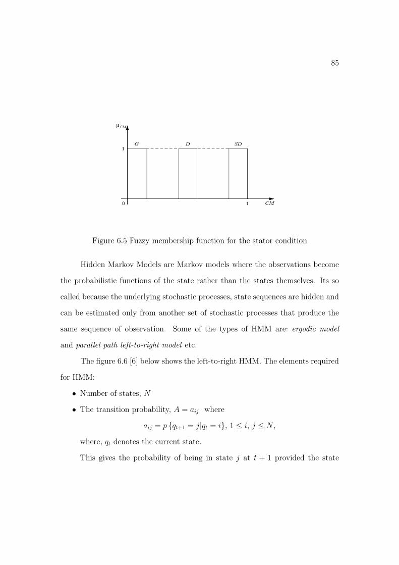
85

Figure 6.5 Fuzzy membership function for the stator condition

Hidden Markov Models are Markov models where the observations become

the probabilistic functions of the state rather than the states themselves. Its so

called because the underlying stochastic processes, state sequences are hidden and

can be estimated only from another set of stochastic processes that produce the

same sequence of observation. Some of the types of HMM are: ergodic model

and parallel path left-to-right model etc.

The figure 6.6 [6] below shows the left-to-right HMM. The elements required

for HMM:

• Number of states, N

• The transition probability, A = aij where

aij = p {qt+1 = j|qt = i}, 1 ≤ i, j ≤ N ,

where, qt denotes the current state.

This gives the probability of being in state j at t + 1 provided the state

86

Figure 6.6 Three state left-to-right Hidden Markov Model

at time t is i. For a stochastic matrix A, the following conditions must be

satisfied:

aij ≥ 0, 1 ≤ i, j ≤ N∑N

j=1 = 1, 1 ≤ i, j ≤ N

Since in the case of left-to-right HMM, the transitions are uni-directional,

the matrix A is upper-triangular.

• Observation probability distribution of each state, B = bj(k), where

bj(k) = pok|qt = j, 1 ≤ j ≤ N , 1 ≤ k ≤ M

ok = kth observation

M = number of distinct observation

These conditions must be satisfied:

bj(k) ≥ 0, 1 ≤ j ≤ N , 1 ≤ k ≤ M

∑Mk=1 bj(k) = 1, 1 ≤ j ≤ N

i.e, the discrete probability should be positive and must sum up to one for

each state. A continuous probability density function for each state must

87

be specified for a continuous observation, in which case a weighted sum of

several Gaussian distributions is used.

bj(ot) =∑M

m=1 cjmN(µjm, Σjm, ot), where cjm = weighter coefficients

µjm = mean vectors

Σjm = covariance matrices

ot = tth observation vector

where, the Gaussian distribution N is given by

N(µjm, Σjm, ot) = e−0.5(ot−µjm)Σ−1

jm(ot−µjm )√

(2π)n|Σjm|

bj(oj)dot is the probability of the jth state generating the observation vector

in the set [ot, ot + dot]. The conditions that need to be satisfied are:

cjm ≥ 0, 1 ≤ j ≤ N , 1 ≤ m ≤ M∑M

m=1 = 1, 1 ≤ j ≤ N

i.e, the weighting coefficients have to be positive and must sum up to one in

each state.

• Initial state distribution, π = πi, where,

πi = pq1 = i, 1 ≤ i ≤ N

i.e, the probability of the ith state being the initial state. These conditions

must be satisfied:

∑Ni=1 πi = 1

i.e, the initial distribution must sum up to one. Since the initial state is

always the first state in case of left-to-right HMMs, therefore, the initial

distribution π is given as [10...0]. The continuous density HMM which is

given by λ is given as:

λ = [A, cjm, µjm, Σjm, π] (6.5)

Some of the problems with HMM are:

88

1. Evaluation Problem: It pertains to the calculation of probability of a set of

O observations, where, O = {o1, o2, o3, ..., oT} for a given Markov Model λ.

Forward-Backward algorithm can be used to calculate the probability.

2. Decoding Problem: It pertains to finding the optimal state sequence of a

HMM, λ for a given set of observations O = {o1, o2, o3, ..., oT}. ”Single best

state sequence” is the most used criteria for defining the optimality, where,

Q = {q1, q2, qT} (this optimal state sequence can be found from Viterbi

algorithm), which maximizes P (Q|O, λ) or P (Q,O|λ).

3. Training Problem: It pertains to finding out the optimal HMM parameters

λ = [A, cjm, µjm, Σjm, π], for a set of observations given as O = {o1, o2, o3, ..., oT}.These parameters can be found from Baum-Welch Algorithm.

6.1.1.4 Neural Network

In the case of linear mapping, the samples in the feature space are projected

in the classification space with the weights of the data sets determined through

known bearing condition. In case of data belonging to the same class, the least

squared criterion is used to create cluster effects. More information on this can be

found from [4]. This however, does not guarantee a clear demarcation of the classes

in the classification space by linear boundaries. There could be an overlapping of

the patterns which belong to different classes in the classification space. This leads

to the necessity of non-linear mapping in the classification space.

A three layered artificial neural network can be used to accomplish non-linear

mapping from the feature space to the classification space. This artificial neural

network represents the non-linear relationship between the input and the output.

The fact that we can develop a non-linear relationship between the input and

the output in the absence of sufficient system information is one of the biggest

89

advantages of using neural networks. Training is the most important aspect of this

neural network structure where most of the intense computation takes place. Once

the training has been done, the network starts working fast for the identification

of any unknown input samples; identifying the relation between any input data

even in the presence of spurious signals.

Artificial Neural Networks(ANN)

Figure 6.7 Multiplayer Neural Network Architecture with two hidden layers

ANN helps in describing a system when it becomes impossible to use analytical

methods. They describe the system in terms of input and output. An ANN

consists of several layers of neurons, an input layer, one or more hidden layers

and an output layer. Details on this can be found in [4]. The output of first

layer (input layer) is fed to the first hidden layer, whose output is fed to the next

90

hidden layer and so on. Figure 6.7 [4] shows the architecture of multiplayer neural

network with two hidden layers.

Figure 6.8 A Neuron Model

A fully connected network is one in which the neuron in one layer is con-

nected to all the neurons or nodes in the previous layer. The signal flows in the

forward direction from layer to layer. Neuron is an information processing unit

for the operation of the neural network. Figure 6.8 [4] shows one such neuron

model. The three elements to the neuron model are:

1. Synapses or connecting links, which is characterized by weight of its own.

For example, a signal xi at the input of synapse i connected to neuron j is

multiplied by the synaptic weight wji, where j is the neuron in question and

i refers to the input end of the synapse.

2. An adder for summing the input signals, weighted by the respective synapses

of the neuron. This forms a linear combiner.

91

3. An activation function which limits the output of a neuron. Except for the

input, every neuron has an activation value which is the weighted sum of the

input signals [4]. The amplitude range of the output signal is limited to some

finite value because of the activation function. Generally, the amplitude

range of the output of a neuron is written as the closed interval [0, 1] or

[−1, 1] [4] Mathematically, neuron j may be described as

uj =I∑

i=1

wjixi (6.6)

and

yi = f(uj − θj) (6.7)

where,

x1, x2, ..., x1 are the input signals

wj1, wj2, ..., wjI are the synaptic weights of the neuron

uj is the linear combiner output

θj is the threshold

f(.) is the activation function

yj is the output signal.

vj, the internal activity level, is the linear combiner output uj modified with

the threshold θj:

vj = uj − θj (6.8)

Equations 6.6 and 6.7 can be combined to give

vj =I∑

i=1

wjixi (6.9)

and

yi = f(vj) (6.10)

92

f(.) is the activation function which denotes the output of a neuron in terms

of the internal activity level at its input. The activation function could be

threshold function, Piecewise-Linear Function and Sigmoid Function.

MultiLayer Feedforward Artificial Neural Network

They are used to solve complicated problems through supervised training with

a popular algorithm called the error back-propagation algorithm. This algorithm

helps in training multilayer perceptrons. Training of feed forward network takes

place in an iterative fashion, where, each iteration cycle involves forward propaga-

tion path followed by an error backward-propagation pass to update the weights [4].

When the input nodes receive their activation function levels in the form of in-

put patterns, the propagation starts, which proceeds through hidden layers up to

the output levels by computing the activation levels of the nodes in each of those

layers. The outputs are produced at the end of it which gives the actual response

of the system. There is no change in the synaptic weight during this propaga-

tion. Weight adjustment is brought by the propagation of the error function of

the output back through the net and modifying all the weights. The iterative

method propagates error function required to adapt weights back from the nodes

in the output layers to nodes in the hidden layers in accordance with the training

rule [4]. In order for the actual response to move closer to the desired response

the weights are adjusted. The adjustments of the training sets are done until the

error criterion is met. Once the training is done, it is possible to relate any input

pattern with an appropriate output pattern. The trained network would give an

output when an input sample is presented to it. A new input would lead to an

output with features that are similar to input vectors with similiar features used

in training. Therefore, the training can be done on a certain set of input/output

pairs without including all the input/output pairs.

93

Back-Propagation Training Algorithm

The NN has to compute the error derivative of the weights in order to train a NN,

so that the error between the desired and actual output is reduced. The derivative

pertains to calculating the error changes as each weight is increased or decreased.

The back propagation algorithm is the most widely used method for computing

this error derivative. It is easiest to understand the back-propagation algorithm

if the network is linear. Each of the error derivatives of the weights is computed

by calculating the error activity, which is the difference between the actual and

desired output. In order to compute the error activity of a hidden unit in the just

before the output layer, all the weights between that hidden unit and the output

units to which it is connected is identified. These weights are then multiplied by

the error activity function of those output units and add the products. This would

give the error activity of the particular hidden unit. We can similarly compute

in like fashion the error activity for other layers, moving from layer to layer in a

direction opposite to the way activities propagate through the network after calcu-

lating all the error activities in the hidden layer just before the output layer, hence,

giving it the name of “back-propagation”. The error derivative of the weight for

each of the incoming connection is calculated once the error activity is calculated.

The Error derivative is the product of the error activity and the activity through

the incoming connection. Gradient descent method is used for implementation of

back-propagation algorithm. The effectiveness and convergence of this algorithm

depends on the value of learning rate constant η. Though gradient descent is an

efficient method for obtaining the weight values that minimizes error, but there

in no constant value of η suitable for all the cases causing errors which reduce the

convergence rate.

94

Radial Basis Function Neural Network (RBFNN)

In case of RBFNN, the activation of the hidden unit is determined by the dis-

tance between the input vector and the prototype vector. It is basically a nearest

neighbor classifier. The structure of a Radial Basis Function is as follows:

f(y, α) = exp(−∑

k |yk − µ|αNθα

) (6.11)

where the exponent parameter α ε (0,∞); and µ and θα are the center and αth

central moment of the data set, respectively. f() becomes Gaussian, for α = 2

which is the typical radial basis function used in the neural network. For any

application, the first task is to calculate the mean and the central moment from the

sampled time series data when the dynamical system is in the nominal condition.

The mean µ and the central moment θα are calculated as:

µ =1

N

N∑

k=1

yk (6.12)

and

θα =1

N

N∑

k=1

|yk − µ|α (6.13)

The distance between any vector y and the center i is obtained as

d (y, µ) ≡ (|y(n)− µ|α)1α (6.14)

From equation 6.11, the RBF at the nominal condition is: f0 = f(y). Under all

conditions, the mean and central moment is constant.

Online Adaptive Reformulation is one of the biggest advantages of using Neural

Networks compared to statistical based methods. This gives it the flexibility which

cannot be achieved through statistical methods. It also eliminates the need for

batch processing. But designing an effective neural network system has always

95

been a challenging task. Back-propagation and RBF give a classification rate of

71.8% and 73.2% respectively [27]. In the case of back-propagation NN, the entire

set of data is used for classification, which eventually becomes a time consuming

process if the data is large, where as, in the case of RBF, the accuracy achieved

is less on account of the dimensioanlity reduction in the data.

Competitive Neural Network

In competitive learning, the output neurons of a NN compete among themselves to

be fired. Details on this can be got from [26]. In case on a NN based on Hebbian

Rule, several of the output neurons may be active at the same time, where as in

competitive learning only a single output neuron is active at any instant of time.

This makes it very useful to discover statistically salient features that can be used

to classify a set of input patterns. The basic elements of a competitive learning

rule are:

• A set of neurons that are same except for the randomly distributed synaptic

weights, and hence give different response to a given set of input patterns.

• A limit imposed on the “strength” of each neuron.

• A mechanism that permits neurons to compete for the right to respond to a

given input, such that only one neuron is active at any given time.

In its simplest form, competitive learning NN has a single layer of output neurons,

each of which is fully connected to the input nodes. For a neuron k to be the

winning neuron, its induced local field vk for a specified input pattern x must

be the largest among all the neurons in the network. The output signal yk of

winning neuron k is set to one; the output signals of all the neurons that lose the

competition are set to 0.

yk = 1 for all j, j 6= k

yk = 0 otherwise

96

where the induced local field vk represents the combined action of all forward and

feedback inputs to neuron k

Let wkj denote the synaptic weight connecting the input node j to neuron k. If

all synaptic weights are positive, then

∑j wkj = 1 for all k

A neuron learns by shifting synaptic weights from its inactive to active input nodes.

Learning does not take place if a neuron does not respond to a particular input

node. If a particular neuron wins the competition, each input node of that neuron

relinquishes some proportion of its synaptic weight, and the weight relinquished

is then distributed equally among the active input nodes [26]. According to the

competitive learning rule, the change (∆wkj) in weight applied to the synaptic

weight (wkj) is given as

∆wkj = η (xj − wkj) if neuron k wins the competition

∆wkj = 0 if neuron k loses the competition

where, η is the learning-rate parameter. This causes the synaptic weight vector

wk of the winning neuron k to move in the direction of the input pattern x. This

neural network also brings about clustering. However, for clustering to happen

in a stable manner, the input patterns must fall into distinct groupings to begin

with; otherwise the network will be unstable. Neural Network has been used in

this thesis because it can handle data which may be distorted and noisy and at

the same time can be used for operation in real time mode.

CHAPTER 7

EXPERIMENTAL RESULTS

Once the analysis of the data is done using a two stage neural network, it is

necessary to evaluate the performance of the fault classifier. This is done through

the performance metrics - Confusion Matrix, Receiver Operating Characteristics

and finally Health Index.

7.1 Implementation

The implementation involves recording the voltage values in the case of

electrical test bed and recording the vibration values for the motor in the case of

mechanical test bed over a period of five days. For recording these values, the test

beds as explained in chapter 2 were used.

7.2 Performance Analysis

7.2.1 Classification of the Input vectors

A classifier maps a list of measured features into a classification state. Figure

7.1 shows the classification of the input data after passing through the artificial

neural network, where the x, y and z axes represent the x, y and z component

of the vibration data respectively. And figure 7.2 shows the classified data for

the electrical test bed, where x and y represent the x and y values of the two

dimensional voltage data. Artificial Neural Network Classifiers implement non-

linear decision boundaries which use ”K-nearest neighbor” discriminant function

analysis to benchmark the neural network’s performance. The nearest neighbor

97

98

classifier can be explained as follows: If it is required to classify an unknown vec-

tor x, where a number of classes are represented by example points in a feature

space vector, then this is done by finding the point closest to x and assigning

the closest point’s class to it. In K-nearest neighbor, nearest K points to x are

found, and x gets assigned the class which is represented by the largest number

of neighboring points. This classification of data paves the way for formulation of

confusion matrix (with the help of testing data) and finally the Receiver Operating

Characteristics. Confusion matrix is used to evaluate the algorithm proposed in

the thesis. Health Index is another method for evaluating the performance of the

machine.

Figure 7.1 Classified Output-Mechanical Test Bed

99

Figure 7.2 Classified Output-Electrical Test Bed

7.2.2 Confusion Matrix

Confusion matrix is a visualization tool used for performance evaluation.

Details on this can be obtained from [27] [50] [51] [52]. It gives a degree of

correlation between various parameters such as features, classes, etc. It is a square

matrix where the entries represent the degree of correlation between its ith and jth

element. The number of rows and columns is equivalent to the number of classes.

The columns represent the system’s classification where as the rows represent the

true classification. For a perfect system, only the diagonal elements will be present

in the confusion matrix, where as, the presence of off diagonal elements indicates

100

misclassification. The sum of all the elements is equal to the number of testing

data. The entries (cij) give the data which are actually of class i but are classified

as class j by the Neural Network System. Thus, it allows the user to understand

the manner in which the classes have been confused with each other. The entries

of the confusion matrix as shown in figure 7.3 is explained as follows:

Figure 7.3 Confusion Matrix

True Positive (TP) gives the number of correct predictions; False Positive

(FP) gives the number of incorrect predictions; False Negative (FN) gives the

number of misses and True Negative (TN) is the number of correct rejections. Out

of all the recorded data, some data sets were chosen for testing the performance of

the two stage neural network. This method of formulating the Confusion Matrix

is called the Generalization Test. After training, the testing data set of known

categories is passed through artificial neural network classification system in order

to find the number of correct and incorrect classifications for each class for getting

101

the TP and FP rates. Figure 7.4 shows the confusion matrix for the testing data

from which the true positive rate (hits) and false positive rate (wrong predictions)

can be determined to get the Receiver Operating Characteristics (ROC) as shown

in figures 7.5 and 7.6.

Figure 7.4 Confusion Matrix of testing data for the Mechanical Test Bed

ROC is a plot of the classifier’s TP rate (sensitivity) against the FP rate

(specificity). Sensitivity is defined as TPTP+FN

and Specificity is defined as FPFP+TN

.

High sensitivity means that the classifier identifies most of the positive samples

and its performance is good, where as high specificity means that the classifier

identifies most of the negative samples and its performance is poor. The curve

always goes through two points (0, 0) and (1, 1). (0, 0) is the point at which no

positives are found by the classifier, where as (1, 1) gives the point where the

classifier finds everything as positive. At (0, 0), the classifier identifies all the

negative cases correctly but the positive cases are identified incorrectly, where as

102

Figure 7.5 Receiver Operating Characteristics of the Mechanical Test Bed

at (1, 1), the classifier identifies all the positive cases correctly but the negative

cases get identified incorrectly. The graph on figure 7.5 shows the ROC for the

mechanical test bed for each of the five days during which the experiment was

performed. Figure 7.6 shows the same for the electrical test bed. It can be clearly

inferred from the graphs that the condition of the motor deteriorates as the days

proceed, i.e, the ROC curve is higher for day 1 compared to day 5. As already

explained, the best performance is achieved near the point (0, 1). The multi-class

task learning vector quantization is reduced to the binary decision, i.e., either it

belongs to a desired class or it does not, irrespective of the number of classes

present.

103

Figure 7.6 Receiver Operating Characteristics of the Electrical Test Bed

7.2.3 Health Index

Health index is also plotted to evaluate the performance of the machine. In

the case of mechanical test bed it is computed by adding weights to various regions

of the metallic disc simulating the faulty bearing, and in the case of electrical test

bed it is done by varying the value of inductance during the course of experiment.

The health index as the name indicates tells the state of the machine under a

particular loading condition. Further information can be obtained from [53]. It

checks the condition of the motor under no load and then uses a fault dictionary to

facilitate the use of pattern recognition techniques to diagnose the faults. Signal

behavior characteristics can be used to study the condition of the motor under no-

load (faultless) and loaded (fault) condition by which we can get the heath index

104

to get the deviation from the normal condition. The health index is calculated

using:

HV (faultless) =

√[(∑

i

(((faultlessi − Yn)/Yn)j × 0.1)2)/(N − 1)] (7.1)

where,

j = 1, 2, 3, ...N

Yn = mean

faultlessi = ith sampled response

Thus, HV (faultless) is the faultless value which acts as the reference for the

system.

For the loaded system (system under fault), the equation would be given by,

HV (fault) =

√[(∑

i

(((faulti − Yn)/Yn)j × 0.1)2)/(N − 1)] (7.2)

The health index if the system can therefore be calculated as

HI = HV (faultless)HV (fault)

if HV (faultless) < HV (fault)

HI = 1 if HV (faultless) > HV (fault)

Figures 7.7 and 7.8 show the health index plot for the mechanical and elec-

trical test bed respectively. It is clear from this figure that the health index would

range between Zero (poor) and 1 (fine), giving an indication of the health of the

system. For the experiments performed in the lab it was found that the health in-

dex was larger for smaller values of weights applied on the inner ring compared to

the larger value of weights which were applied on the outer ring, in the case of me-

chanical test-bed; and it was larger for smaller value of inductances as compared to

the larger values of inductances in the case of electrical test-bed. This also implies

that the vibrations produced are lesser when the weights are applied on the inner

105

Figure 7.7 Health Index for the Mechanical Test Bed

ring as opposed to those applied on the middle and outer rings respectively in the

case of mechanical test bed experimentation. Similarly, the value of fault voltage

obtained is greater when the value of the external inductance added is higher in

value as in the case of electrical test bed. This would help condition monitoring

systems to be implemented, where maintenance action can be brought into service

at some predetermined value of failure. During failure, the latest response can be

assigned as the cause for diagnosis. The trend obtained from this polt can be used

for fault prognosis.

106

Figure 7.8 Health Index for the Electrical Test Bed

CHAPTER 8

CONCLUSION AND FUTURE WORK

This research work proposes diagnosis and prognosis of bearing faults and

stator winding faults using Wireless Modules and Wireless Sensors, where in, a

novel two stage neural network has been used to analyze the vibration data and

the voltage values obtained from the mechanical and electrical test-bed setup re-

spectively. The work suggests an experimental setup which is a low cost approach

for emulating bearing fault and short circuit current fault in a motor; to wire-

lessly sense the vibrations and voltages produced due to these faults. The fault

classification algorithm used has certain features such as: (a) Using PCA rather

than conventional statistical methods to reduce the dimensionality of the data,

(b) A method which estimates and recursively calculates the principal compo-

nents, hence, giving robustness in the diagnosis, (c) Use of Supervised Learning

Quantization which has a fast processing time, (d) Finally, Receiver Operating

Characteristics is plotted and the health index is computed to find the condition

of the motor at a given instant. One of the features that could be used in the

future is the use of energy efficient wireless sensors and modules in order to make

the Condition Based Maintenance more effective. The sampling rate of the wire-

less modules for vibration and voltage measurement could be increased further by

using a SD card which would store the values and then transmit to the computer;

The vibration measurement is basically the measurement of sound, so there could

be better reproduction of the signals obtained from the machine if a wireless mod-

ule is programmed with a sampling rate of more than 7K (Nyquist Criterion).

107

108

Since, in the measurement of vibration, the value of g(center of gravity) plays a

very significant role, comparative studies can be done if the entire experiment is

done in a new environment as this would give a set of values with different center

of gravity-giving the extent to which the center of gravity has an effect on the

readings, this could also show the effect of external parameters on the readings

obtained. In this thesis we have considered only two type of faults in the induc-

tion motor- one each for electrical and mechanical. We could also consider other

fault types to determine the classifier performance for indicating the condition of

the motor at any instant of time. Last, the experiment has been conducted on

induction motor since its widely used in the industry and has simple and rugged

construction, we could examine the classifier performance by performing the ex-

periments on other types of motor like the synchronous motor.

REFERENCES

[1] A. Tiwari, P. Ballal, and F. L. Lewis, “Energy-efficient wireless sensor network

design and implementation for condition-based maintenance,” vol. 1, 2007,

pp. 1–23.

[2] P. Ballal and F. Lewis, Wireless Sensor Network Design. Pearson Education,

to be published.

[3] http://www.bmpcoe.org/bestpractices/internal/arlps/arlps7.html.

[4] C. Ping, “Bearing condition monitoring and fault diagnosis,” Master’s thesis,

University of Calgary (Canada), 2001.

[5] R. Samsi, “A probabilistic framework for fault detection in induction motors,”

Ph.D. dissertation, The Pennsylvania State University, 2006.

[6] O. Hasan, “Fault detection, diagnosis and prognosis of rolling element bear-

ings: Frequency domain methods and hidden markov modeling,” Ph.D. dis-

sertation, Case Western Reserve University, 2004.

[7] P. D. McFadden and J. D. Smith, “Model for the vibration produced by

a single point defect in a rolling element bearing,” Journal of Sound and

Vibration, pp. 69–82, 1984.

[8] H. R. Martin and F. Honarvar, “Application of statistical moments to bearing

failure detection,” vol. 44, 1995, pp. 67–77.

[9] R. B. W. Heng and M. J. M. Nor, “Statistical analysis of sound and vibration

signals for monitoring rolling element bearing condition,” vol. 53, 1998, pp.

211–226.

109

110

[10] P. D. McFadden and J. D. Smith, “Vibration monitoring of rolling element

bearings by high frequency resonance technique-a review,” vol. 77, 1984, pp.

3–10.

[11] I. Howard, “A review of rolling element bearing vibration: Detection, diag-

nosis and prognosis,” 1994.

[12] E. A. Seyfettin, “Multisensor fusion for induction motor aging analysis and

fault diagnosis,” Ph.D. dissertation, The University of Tennessee, 1999.

[13] C. J. Li and J. Ma, “Wavelet decomposition of vibrations for detection of

bearing localized faults,” vol. 30, 1997, pp. 143–149.

[14] ——, “Bearing localization defect detection by bicoherence analysis of vibra-

tions,” Journal of Engineering for Industry, vol. 117, pp. 625–629, 1995.

[15] G. Godi, B. Li, M. Y. Chow, and J. C. Hung, “Motor bearing diagnosis by a

fundamental frequency amplitude based fuzzy decision system,” vol. 4, 1998,

pp. 1961–1965.

[16] Vibration analysis via neural network inverse models to determine aircraft

engine unbalance condition, vol. 4, 2003.

[17] I. E. Alguindigue, A. Loskiewicz-Buczak, R. E. Uhrig, L. Hamon, and

F. Lefevre, “Vibration monitoring of edf rotating machinery using artificial

neural networks,” 1991.

[18] D. H. Hanson, “Artificial neural network based survival analysis for hydro-

mechanical systems,” Ph.D. dissertation, The University of Iowa, 2004.

[19] M. Subrahmanyam and C. Sujatha, “Using neural networks for the diagnosis

of localized defects in ball bearings,” vol. 30, 1997, pp. 739–752.

[20] http://images.google.com/imgres?imgurl=http://mvpprograms.com/help/images/KurtosisPict.

[21] L. I. Smith, A tutorial on Principal Component Analysis.

111

[22] M. H. Fredric and K. Ivica, Principles of Neurocomputing for Science and

Engineering. McGraw-Hill.

[23] M. A. Turk and A. P. Pentland, “Face recognition using eigenfaces,” pp.

586–591.

[24] ——, “Eigenfaces for recognition,” vol. 3(1), 1991.

[25] T. Sanger, “Optimal unsupervised learning in a single layer linear feedforward

neural network,” vol. 12, 1989, pp. 459–473.

[26] S. Haykin, Neural Networks A Comprehensive Foundation. Pearson Educa-

tion, 2003.

[27] P. S. Dang, “A potential field approach for distributed control of discrete

actuator and sensor arrays,” Ph.D. dissertation, University of Texas at Ar-

lington, 2007.

[28] S. Chitroub, A. Houacine, and B. Sansal, “Principal component analysis of

multispectral images using neural networks,” pp. 89 – 95.

[29] E. Oja, “Neural networks principal components and subspaces,” Intenational

Journal of Neural Systems, pp. 61–68, 1989.

[30] ——, “A simplified neuron model as a principal components analyzer,” Jour-

nal of Mathematical Biology, pp. 267–273, 1989.

[31] http://www.cs.helsinki.fi/u/ahyvarin/whatisica.shtml.

[32] V. J. Stone, Independent Component Analysis: A Tutorial Introduction.

[33] J. Shlens, A tutorial on Principal Component Analysis.

[34] M. T. Hagan, H. B. Demuth, and M. Beale, Neural Network Design. PWS

Publishing Company.

[35] http://www.statsoft.com/textbook/glosc.htmlClassification.

[36] http://www.gc.ssr.upm.es/inves/neural/ann1/concepts/Suunsupm.htm.

[37] http://pagesperso-orange.fr/polyvalens/clemens/wavelets/wavelets.html.

112

[38] http://www.astro.princeton.edu/esirko/idlhtmlhelp/examples3.html.

[39] F. A. K. A. Badour, “Application of wavelet techniques to vibration analysis

of rotating machines,” Master’s thesis, King Fahd University of Petroleum

and Minerals, December 2007.

[40] S. Bhunia, K. Roy, and J. Segura, “A novel wavelet transform based transient

current analysis for fault detection and localization,” New Orleans Louisiana

USA, 2002, pp. 0–412.

[41] I. Daubechies, Ten Lectures on Wavelets, ser. CBMS-NSF Reg. Conf. Ser.

Appl. Math. 61. Philadelphia, PA: SIAM, 1992.

[42] R. Rao and A. Bopardikar, Wavelet Transforms: Introduction to Theory and

Applications Reading. Massachussets, MA: Addison-Wesley, 1998.

[43] M. E. H. Benbouzid and H. Nejjari, “A simple fuzzy logic approach for in-

duction motors stator condition monitoring,” 2001, pp. 634 – 639.

[44] D. Sauter, N. Mary, F. Sirou, and Thieltgen, “Fault diagnosis in systems

using fuzzy logic,” vol. 2, 1994, pp. 883 – 888.

[45] A fuzzy diagnostic System: application to linear induction motor drives,

vol. 1, 1997.

[46] G. G. et al., “Motor bearing fault diagnosis by a fundamental frequency

amplitude based fuzzy decision system,” vol. 4, 1998, pp. 1961–1965.

[47] M. Zeraoulia, A. Mamoune, H. Mangel, and M. E. H. Benbouzid, “A sim-

ple fuzzy logic approach for induction motors stator condition monitoring,”

Journal of Electrical Systems, pp. 15–25, 2005.

[48] J. M. Mendel, “Fuzzy logic systems for engineering: a tutorial,” vol. 83, 1995,

pp. 345–377.

[49] A. W. Drake, Fundamentals of Applied Probability Theory. NewYork:

McGraw-Hill Company, 1967.

113

[50] A. Zaknich, Neural networks for intelligent signal processing: World Scientific

Singapore. John Wiley and Sons Inc., 2003.

[51] G. Vachtsevanos, F. Lewis, M. Roemer, A. Hess, and B. Wu, Intelligent Fault

Diagnosis and Prognosis for Engineering Systems. John Wiley and Sons

Inc., 2006.

[52] C. Chen, Signal and image processing for remote sensing. CRC Press Tech-

nology and Industrial Arts, 2006.

[53] A. Davies, Handbook of Condition Monitoring: Techniques and Methodology.

Chapman and Hall, 1998.

BIOGRAPHICAL STATEMENT

Akarsha Ramani received her Bachelor of Engineering degree in Electrical

and Electronics Engineering from Anna University, 2005. She pursued her Master

of Science in University of Texas at Arlington, where she worked as a Graduate

Research Assistant at Automation and Robotics Research Institute.

114