Mutual diffusion in the ternary mixturewater + methanol + ethanol and its binary subsystems

Stanislav Parez,1 Gabriela Guevara-Carrion,2 Hans Hasse2 and Jadran Vrabec3a

1 Institute of Chemical Process Fundamentals, Academy of Sciences of the Czech Republic,165 02 Prague, Czech Republic.

2 Laboratory for Engineering Thermodynamics, University of Kaiserslautern, 67663Kaiserslautern, Germany.

3 Thermodynamics and Energy Technology, University of Paderborn, 33098 Paderborn,Germany.

Keywords: Fick diffusion, Maxwell-Stefan diffusion, thermodynamic factor, molecular simu-lation, Taylor dispersion, water, methanol, ethanol

Abstract

Mutual diffusion is investigated my means of experiment and molecular simulation for liquidmixtures containing water + methanol + ethanol. The Fick diffusion coefficient is measuredby Taylor dispersion as a function of composition for all three binary subsystems at ambientconditions. For the aqueous systems, these data compare well with literature values. In case ofmethanol + ethanol, experimental measurements of the Fick diffusion coefficient are presentedfor the first time. The Maxwell-Stefan diffusion coefficient and the thermodynamic factor arepredicted for the ternary mixture as well as its binary subsystems by molecular simulationin a consistent manner. The resulting Fick diffusion coefficient is compared to present mea-surements and to the classical simulation approach, which requires experimental vapor-liquidequilibrium or excess enthalpy data. Moreover, the self-diffusion coefficients and the shearviscosity are predicted by molecular dynamics and are favorably compared to experimentalliterature values. The presented ternary diffusion data should facilitate the development ofaggregated predictive models for diffusion coefficients of polar and hydrogen-bonding systems.

a To whom correspondence should be addressed, Email: jadran.vrabec@upb.de

1

1 Introduction

The chemical industry has a need for accurate thermodynamic properties of mixtures in gen-eral1. Almost all separation processes in chemical engineering, such as distillation, absorptionor extraction, are affected by diffusion in liquids. Diffusion may even be the rate determiningprocess in mass transfer unit operations2 so that knowledge of the mutual diffusion coefficientsis required for their design and optimization3.

To determine diffusion coefficients, experimental methods, molecular simulation, theoret-ical or empirical approaches are used. Numerous theoretical and empirical approaches topredict mutual diffusion coefficients in multicomponent mixtures can be found in the liter-ature1,4–7. However, these approaches often fail in predictive applications, especially whenhighly polar and hydrogen-bonding liquids are considered, because they relate mutual dif-fusion coefficients to one-component properties or simplify the interaction between unlikemolecules. In this context, molecular simulation offers a promising alternative for predictingmutual diffusion coefficients.

Two rigorous descriptions of diffusive mass transport in multicomponent liquids are com-monly used: generalized Fick’s law and Maxwell-Stefan (MS) theory5. Fick’s law relates adiffusive flux to a gradient of a measurable quantity, e.g. a mole fraction, whereas in MStheory, the driving force is the gradient of the chemical potential so that the MS diffusioncoefficient is not directly accessible by experiment. The MS diffusion coefficient can be calcu-lated by equilibrium molecular dynamics (EMD) simulation from velocity correlation functions(Green-Kubo formalism) or, alternatively, via the Einstein formalism5,8. The thermodynamicfactor serves as a conversion factor between both mutual diffusion coefficient types. Therefore,knowledge of the thermodynamic factor is required to determine the Fick diffusion coefficienton the basis of EMD simulation. It should be noted that the mutual diffusion coefficients andthe thermodynamic factor are matrices for mixtures containing three or more components.

The thermodynamic factor is usually estimated from experimental vapor-liquid equilibrium(VLE) or excess enthalpy data9,10, employing an equation of state, like Soave-Redlich-Kwongor PC-SAFT, or an excess Gibbs energy GE model, such as Margules, Van Laar, Wilson,NRTL, UNIQUAC or UNIFAC. Some examples can be found in11–16. However, this classicalapproach suffers from two drawbacks. First, the thermodynamic factor highly depends onthe underlying thermodynamic model, because different GE models may describe VLE dataequally well, but yield significantly different values for the thermodynamic factor10,17. Thehigh uncertainty related to the thermodynamic factor from a thermodynamic continuum modelthat was regressed to VLE data has been recognized by many authors9,10,12,18. Second, thethermodynamic factor determined by this approach corresponds to thermodynamic conditionsunder which VLE data were measured. These conditions usually differ from those where thethermodynamic factor is needed for the conversion between the mutual diffusion coefficienttypes.

In recent years, there has been a growing effort to obtain the thermodynamic factor di-rectly from molecular simulation. E.g., it can be estimated directly from the integration ofthe radial distribution function with respect to the distance using the Kirkwood-Buff the-ory19,20. This method has some drawbacks because of the presence of strong fluctuations atlarge distances, thus, very large systems are required and it is difficult to obtain good statis-tics21,22. Wedberg et al.23–25 describe a method for extending radial distribution functionsthat allows the Kirkwood-Buff integrals to be calculated from simulations of relatively smallsystems. Schnell et al.26–28 developed a method to compute the thermodynamic factor using

2

the Kirkwood-Buff integrals that were obtained from density fluctuations in small subsystemsembedded in a larger simulation box using EMD simulations. They used the formalism ofHill29 to obtain a finite size scaling factor, here the different boundary conditions of smallperiodic and non-periodic systems were accounted for by adding an effective surface energyterm26. This approach has been tested by Schnell et al.26 for binary mixtures of WCA andLennard-Jones fluids and by Liuet al. for the binary liquid mixtures acetone + methanoland acetone + tetrachloromethane30, as well as for the ternary liquid mixture chloroform +acetone + methanol31.

Another molecular simulation approach is to determine the composition dependence of thechemical potential using free energy perturbation methods like Widom’s particle insertion14.Recently, Balaji et al.32 proposed a modification of the Widom method33 to compute thethermodynamic factor from a single simulation for mixtures of Lennard-Jones fluids.

In this work, the thermodynamic factor was calculated from the composition dependence ofthe chemical potential at constant temperature and pressure by Monte Carlo (MC) simulation.Because this approach is (for dense liquids) challenging with respect to the quality of molecularmodels, the technique used for the calculation of the chemical potential and the availabilityof high performance computing resources, it has often been avoided. The aim of this workis to show that the current capabilities of molecular simulation meet this challenge even forstrongly polar and hydrogen-bonding liquids like aqueous alcohol mixtures.

Experiments provide the Fick diffusion coefficient on the basis of a variety of usuallytime consuming techniques from optical interferometry to NMR spin relaxation34. The mostfrequently applied methods are interferometry, the diaphragm cell and Taylor dispersion, whichis also known as peak broadening technique. In Taylor dispersion35,36, a laminar flow of acarrier solution is pumped through a long capillary tube. A pulse of the same solution witha slightly different composition is injected. Convection and diffusion in the laminar capillaryflow lead to a distortion of the peak which takes the form of a Gaussian distribution of theconcentration37. The Fick diffusion coefficient is calculated from the resulting concentrationprofile that is measured at the end of the capillary tube. This method was used in this workbecause it is relatively fast (1 to 3 h per experimental point) and requires a rather simpleexperimental set-up.

The systems under study, i.e. the ternary mixture water + methanol + ethanol and itsbinary subsystems, are highly polar hydrogen-bonding liquids, which are challenging from thepoint of view of both simulation and experiment. Molecular simulation results are provided forseveral transport properties, i.e. MS and Fick diffusion coefficients, self-diffusion coefficientsand shear viscosity. Furthermore, experimental results for the Fick diffusion coefficient aregiven for all binary subsystems. In particular, experimental Fick diffusion coefficient data ofmethanol + ethanol are presented here for the first time.

Although binary data on the Fick diffusion coefficient are relatively abundant, experimentaldata on diffusion of ternary and quaternary mixtures are scarce13,38, which is mainly becauseof experimental difficulties. Recently, Wambui Mutoru and Firoozabadi38 made a literaturesurvey on diffusion coefficient data for mixtures containing three or more components. Theyfound experimental data points for only 94 ternary and 13 quaternary mixtures, where mostof them contain water. Moreover, only data at ambient pressure and temperatures between286 and 323 K have been reported. Unfortunately, the ternary mixture water + methanol +ethanol was not yet studied by experiment.

The number of molecular simulation studies on transport properties for complex liquids

3

is still low. Simulation works on mixtures containing three or more components are almostabsent. Typically, aqueous solutions of methanol39–43 or ethanol22,39,43–46 have been studiedby EMD simulation. Nevertheless, most of these works investigate the self-diffusion coefficientand leave aside mutual diffusion, which is more demanding than self-diffusion. For the mix-ture methanol + ethanol, transport properties, including the MS diffusion coefficient, werecalculated in our preceding work47. Non-equilibrium molecular dynamics simulations havealso been applied to determine the shear viscosity for aqueous alcohols43,48,49. However, non-equilibrium simulations are difficult to evaluate regarding diffusion, because they require veryhigh concentration gradients beyond the linear response regime.

The success of molecular simulation to predict thermodynamic properties is primarily de-pendent on the molecular model that describes the intermolecular interactions. In this work,rigid, united-atom type models were used. The models for both alcohols were developed inour group50,51; for water, the TIP4P/2005 model52 was taken from the literature. Thesemodels were tested in our previous works with respect to the binary mixtures under consider-ation39,47,48 and successfully reproduced the experimental values of transport properties in thewhole composition range without a need for introducing additional parameters to adjust theinteraction between unlike components. Furthermore, the TIP4P/2005 model was appreciatedby many authors to be the most successful among the rigid, non-polarizable water models withrespect to various structural and transport properties39,53–55.

This paper is organized as follows. In section 2, the methods for the determination ofthe Fick diffusion coefficient from molecular simulation and experiment are described. Theemployed molecular models and the technical simulation details are introduced in sections 3and 4. The experimental details are described in section 5. In section 6, results from simulationand experiment are presented and discussed. Finally, conclusions are drawn.

2 Methodology

To describe mass transport in liquid mixtures, Fick’s law and MS theory are used. Fick’s law5

relates a mass flux to a gradient of a driving force causing this flux. In this case, the drivingforce is given in terms of the gradient of a mole fraction ∇xj. The diffusive molar flux Ji ofcomponent i is

Ji = −ρn−1∑j=1

Dij∇xj , i = 1 . . . n− 1, (1)

where n is the number of components in the mixture, ρ is the molar density of the mixtureand Dij denotes the Fick diffusion coefficient that couples the flux of component i with thegradient of the mole fraction of component j. Because the molar fluxes depend on a choice ofthe reference frame, the diffusion coefficients are defined accordingly. In this work, the averagemolar velocity frame was used, which propagates with respect to the laboratory frame withthe velocity

u =n∑

i=1

xiui , (2)

4

where ui is the average velocity of component i in the laboratory frame. For this choice,∑ni=1 Ji = 0 holds. Hence, the molar flux of the reference component n is obtained from the

flux balance and there are (n− 1)2 independent Fick diffusion coefficients.

In MS theory5, the driving force is the gradient of the chemical potential ∇µi, which isassumed to be balanced by a friction force that is proportional to the mutual velocity betweenthe components

−β∇µi =n∑

j 6=i=1

xj(ui − uj)−Dij

, (3)

where β = 1/(kBT ) is the Boltzmann factor. The MS diffusion coefficient −Dij thus playsthe role of an inverse friction coefficient between components i and j. MS diffusivities aresymmetric −Dij = −Dji so that there are n(n− 1)/2 independent MS diffusion coefficients.

Because Eqs. (1) and (3) describe the same phenomenon, a relation between both sets ofdiffusion coefficients exists5

D = B−1Γ , (4)

in which all three symbols represent (n−1)×(n−1) matrices. D is the matrix of Fick diffusioncoefficients Dij, the elements of the matrix B are given by

Bii =xi

−Din

+n∑

j 6=i=1

xj−Dij

, Bij = −xi(

1−Dij

− 1−Din

), (5)

and the so-called matrix of the thermodynamic factor Γ is defined by

Γij = δij + xi∂ ln γi∂xj

∣∣∣∣T,p,xk,k 6=j=1...n−1

, (6)

where δij is the Kronecker delta and γi is the activity coefficient of component i.

For binary mixtures, Eq. (4) reduces to the scalar relation

D = −DΓ , (7)

because there is only a single independent MS and Fick diffusion coefficient. Here,

Γ = 1 + x1d ln γ1dx1

= 1 + x2d ln γ2dx2

. (8)

The MS diffusion coefficient can be transformed to the Fick diffusion coefficient and viceversa if the thermodynamic factor is known. Only the Fick diffusion coefficient can be mea-sured experimentally, whereas only the MS diffusion coefficient can be obtained directly fromEMD simulation.

5

2.1 Molecular Simulation

The Fick diffusion coefficient was determined consistently by means of molecular simulation.In particular, both the MS diffusion coefficient and the thermodynamic factor were computed.As discussed above, the latter is usually derived from experimental VLE data, despite thefact that this method suffers from inaccuracies. In the present method, the thermodynamicfactor was calculated straightforwardly following its definition (6). The chemical potentials,and thus the activity coefficients, were sampled by MC simulation. The derivatives of theactivity coefficients at constant temperature and pressure were subsequently obtained froma fit of the simulation results using a thermodynamic model. Having the thermodynamicfactor, the MS diffusion coefficients, as determined by EMD simulation, were transformed tothe Fick diffusion coefficients according to Eq. (4). It will be shown that with an appropriatemethod and suitably chosen parameters, the composition profile of the chemical potentialscan be obtained by relatively inexpensive simulations (using efficient molecular models) moreplausibly than with the method based on experimental VLE data.

Transport Properties

EMD simulation and the Green-Kubo formalism56,57 were used here to calculate transportproperties. This formalism establishes a direct relationship between a transport coefficientand the time integral of the auto-correlation function of the corresponding microscopic flux ina system under equilibrium.

For the MS diffusion coefficient, the relevant Green-Kubo expression is based on the netvelocity auto-correlation function6

Lij =1

3N

∫ ∞

0

dt⟨ Ni∑

k=1

vi,k(0) ·Nj∑l=1

vj,l(t)⟩, (9)

where N is the total number of molecules, Ni is the number of molecules of component i andvi,k(t) denotes the velocity of k-th molecule of component i relative to the molar averaged frameof reference at a time t58 that was used in the definition of the Fick diffusion coefficient (2).The MS diffusion coefficient in binary mixtures is defined by6

−D =x2x1L11 +

x1x2L22 − L12 − L21 . (10)

For a ternary mixture, the B−1 matrix that represents the MS contribution to mutual diffu-sivity, cf. Eqs. (4) and (5), reads

B−111 = (1− x1)

(L11

x1− L13

x3

)− x1

(L21

x1− L23

x3+L31

x1− L33

x3

),

B−112 = (1− x1)

(L12

x2− L13

x3

)− x1

(L22

x2− L23

x3+L32

x2− L33

x3

),

B−121 = (1− x2)

(L21

x1− L23

x3

)− x2

(L11

x1− L13

x3+L31

x1− L33

x3

),

B−122 = (1− x2)

(L22

x2− L23

x3

)− x2

(L12

x2− L13

x3+L32

x2− L33

x3

). (11)

6

Beside the MS diffusion coefficient, the self-diffusion coefficient and the shear viscosity weresampled. The self-diffusion coefficient Dself

i is related to the mass flux of a single molecule ofcomponent i within a fluid. Therefore, the relevant Green-Kubo expression is based on theindividual molecule velocity auto-correlation function59

Dselfi =

1

3Ni

∫ ∞

0

dt

Ni∑k=1

⟨vi,k(t) · vi,k(0)

⟩. (12)

Because all molecules of a given species contribute to the self-diffusion coefficient, the auto-correlation function is averaged over all Ni molecules of component i. Thereby, a betterconvergence than in case of Lij is achieved. This is favorable in connection with some classicalpredictive approaches, such as the Darken model, that estimate the MS diffusion coefficient onthe basis of self-diffusion coefficients. The Darken model considers only the self-correlationsin Eq. (9), resulting for binary mixtures to60

−D = x1Dself2 + x2D

self1 . (13)

Hence, the Darken model is applicable for ideally diffusing mixtures, where the contributionof the velocity cross-correlations to the net velocity auto-correlation function is negligible30.Recently, Liu et al.61 proposed a model which requires only self-diffusion coefficients at infinitedilution to parameterize Eq. (13)

1

Dselfi

=n∑

j=1

xjlimxj→1Dself

i

. (14)

Diffusivity is often discussed in the context of viscous properties. The shear viscosity η, asdefined by Newton’s ”law”, is associated with the momentum transport under the influenceof velocity gradients. Hence, the shear viscosity can be related to the time auto-correlationfunction of the off-diagonal elements of the stress tensor Jxy

p59

η =β

V

∫ ∞

0

dt⟨Jxyp (t) · Jxy

p (0)⟩, (15)

where V stands for the molar volume. Averaging over all three independent elements of thestress tensor, i.e. Jxy

p , Jxzp and Jyz

p , improves the statistics of the simulation. The componentJxyp of the microscopic stress tensor Jp is given by62

Jxyp =

N∑i=1

mivxi v

yi −

1

2

N∑i=1

N∑j 6=i

l∑a=1

m∑b=1

rxij∂uij∂ryab

. (16)

Here, the lower indices a and b count the interaction sites and the upper indices x and ydenote the spatial vector components. The index denoting a component is omitted, becausethe summation is carried out over all molecules regardless of their species. Finally, mi is themass of molecule i.

7

Chemical Potential

The chemical potential µi of component i can be separated into the solely temperature depen-dent ideal contribution µid

i (T ) and the remaining contribution µi(T, p,x) ≡ µi(T, p,x)−µidi (T ).

This contribution contains the desired ln γi term that appears in Eq. (6)

βµi(T, p,x) ≡ ⵕi (T, p) + lnxi + ln γi(T, p,x) ,

where • denotes a pure component property. Thus, the solely temperature dependent idealcontribution does not need to be determined for the present purpose.

The composition derivative of the activity coefficient becomes

∂ ln γi∂xj

∣∣∣∣T,p,xk,k 6=j=1...n−1

=∂(βµi − ln xi)

∂xj

∣∣∣∣T,p,xk,k 6=j=1...n−1

. (17)

This derivative was calculated here analytically from the Wilson model10 that was fitted topresent simulation data of βµi − lnxi

βµi − ln xi = βMi + 1− lnSi −n∑

k=1

xkΛki/Sk , i = 1 . . . n , (18)

Si =n∑

k=1

xkΛik , Λii = 1 ,

where Mi and Λij for i 6= j are adjustable parameters. The parameter Mi stands for thechemical potential of the pure component i, while Λij is related to the change of the chemicalpotential of component i with respect to the mole fraction of component j. The diagonalterms Λii are constrained to be unity. In a ternary mixture, there are thus nine parameters tofit the three chemical potentials with the Wilson model: three Mi and six Λij.

Inserting Eq. (18) into Eq. (6) using Eq. (17) yields the thermodynamic factor

Γij = δij + xi(Qij −Qin) , (19)

Qij = −Λij/Si − Λji/Sj +n∑

k=1

xkΛkiΛkj/S2k .

Note that the thermodynamic model of a n-component mixture determines the propertiesof its subsystems. As a consequence, once the Wilson model for a ternary mixture is available(Eq. (18) with n = 3), the properties of all binary subsystems can be expressed in terms ofmole fractions and the parameters of the model corresponding to the selected two components.E.g., the thermodynamic factor of the binary mixture of components i and j is determined by(only two) parameters of the ternary model, i.e. Λij and Λji,

8

Γ = 1 + xid ln γidxi

= 1 + xi(Qii −Qij) =

= 1 + xi

(−2 + Λij

xi + xjΛij

+Λji

xj + xiΛji

+ xi1− Λij

(xi + xjΛij)2+ xjΛji

Λji − 1

(xj + xiΛji)2

).

(20)

2.2 Experiment

A fluid flowing through a tube develops a velocity profile which is a function of the radialposition. In a fully developed laminar flow, Newtonian fluids propagate with a parabolicvelocity profile. When a pulse of a solution with a different composition is injected into alaminar carrier solution flow, it propagates with the carrier flow velocity that corresponds toits position in the tube cross section63. This leads to a radial concentration gradient whichin turn causes radial diffusion. The molecules at the pulse front near the tube axis diffusetowards the wall into streamlines with a lower flow velocity and the molecules near the walldiffuse towards the center of the tube into streamlines with a higher flow velocity. These radialmotions become important if they are of the same order of magnitude as the convective axialmotion, i.e. when the axial flow velocity is low or the radial distances are small64. At the endof the capillary tube, the pulse exhibits an axial Gaussian concentration profile35,65.

The mathematical description of this process in binary mixtures is given by2

D

[∂2ci∂z2

+1

r

∂ci∂r

+∂2ci∂r2

]=∂ci∂t

+ U0

(1− r2

R2

)∂ci∂z, (21)

where D is the binary Fick diffusion coefficient, ci the molarity of component i and U0 is thevelocity maximum at the center of the tube with an internal radius R. t is the time, r and zare the radial and axial coordinates, respectively.

Taylor35 used a set of assumptions to find a solution for Eq. (21). He assumed that atlow laminar flow rates transport via axial diffusion is small compared to the transport viaconvection, and that the length of the capillary tube is much larger than its diameter2. Whena Dirac δ-pulse is injected into the carrier solution, the shape of the dispersed pulse can thenbe related to a dispersion coefficient k by35

∆ci (t) =∆ne

2πR2√πkt

exp

[−L2 (1− t/τ)2

4kt

]· (22)

Here, ∆ci (t) is the temporal change in concentration of component i, ∆ne is the excess numberof moles present in the pulse solution when compared to the carrier solution, L is the lengthof the capillary tube and τ is the mean residence time. The dispersion coefficient is related tothe Fick diffusion coefficient D by65

k = D +R2L2

48τ 2D· (23)

If D is very small, the dispersion coefficient simplifies to36

9

k =R2L2

48τ 2D· (24)

Aris65 proposed another solution to Eq. (21) that employs the first

t =

∞∫0

dt∆cit

∞∫0

dt∆ci

, (25)

and second

σ2 =

∞∫0

dt (t− t)2∆ci

∞∫0

dt∆ci

, (26)

moments of the concentration distribution. The Fick diffusion coefficient is then given by

D =R2t

24σ2· (27)

3 Molecular Models

Throughout this work, rigid, non-polarizable molecular models of united-atom type were used.These simple models account for the intermolecular interactions, including hydrogen-bonding,by a set of Lennard-Jones (LJ) sites and point charges which may or may not coincide withthe LJ site positions. The potential energy uij between two molecules i and j can thus bewritten as

uij (rijab) =l∑

a=1

m∑b=1

4εab

[(σabrijab

)12

−(σabrijab

)6]+

qiaqjb4πε0rijab

,

where a is the site index of molecule i, b the site index of molecule j, while l and m indicatethe number of interaction sites of molecules i and j, respectively. rijab represents the site-sitedistance between molecules i and j. The LJ size and energy parameters are σab and εab. qiaand qjb are the point charges located at the sites a and b of the molecules i and j, whereas ε0is the permittivity of vacuum.

For water, the TIP4P/2005 model by Abascal and Vega52 was used here. It consists of oneLJ site and three point charges. The molecular models for methanol and ethanol were takenfrom prior work50,51 of our group. They consist of two (methanol) or three (ethanol) LJ sitesand three point charges each. All models are simple, i.e. they do not consider internal degreesof freedom and also do not cover the polarizability in an explicit way. The interested readeris referred to the original publications50–52 for detailed information about the three molecularpure substance models and their parameters.

10

To define a molecular model for a binary mixture on the basis of pairwise additive puresubstance models, only the unlike interactions have to be specified. In case of polar interactionsites, i.e. point charges here, this can straightforwardly be done using the laws of electrostatics.However, for the unlike LJ parameters, there is no physically sound approach so that combiningrules have to be employed for predictions. Here, the interactions between unlike LJ sites oftwo molecules were determined by the simple Lorentz-Berthelot combining rule

σab =σaa + σbb

2,

and

εab =√εaaεbb .

The mixture data presented below are strictly predictive, because not a single experimentaldata point on mixture properties or on transport properties was considered in the modelparameterization.

4 Simulation Details

All simulations were carried out in a cubic volume with periodic boundary conditions. Electro-static long-range corrections were considered by the reaction field technique with conductingboundary conditions (εRF = ∞). The statistical uncertainties of the predicted values wereestimated with a block averaging method66.

Transport Properties

EMD simulations were performed with the program ms267. These were done in two steps:first, a simulation in the isobaric-isothermal (NpT ) ensemble was carried out to calculatethe density at the desired temperature, pressure and composition. Second, a canonic (NV T )ensemble simulation was carried out to determine the MS and self-diffusion coefficient as wellas the shear viscosity at the temperature, composition and density from the first step.

The simulations in the NpT ensemble were equilibrated over 8×104 time steps, followed bya production run over 7×105 time steps. The NV T simulations were equilibrated over 8×104

time steps, followed by production runs of 9 to 14 × 106 time steps. The MS and the self-diffusion coefficients were calculated with Eqs. (10) to (12) using up to 7 × 104 independenttime origins of the auto-correlation functions. The sampling length of the auto-correlationfunctions was 13 ps. The separation between the time origins was chosen such that all auto-correlation functions have decayed at least to 1/e of their normalized value to achieve theirtime independence68.

In all EMD simulations, Newton’s equations of motion were solved using a fifth-orderGear predictor-corrector numerical integrator with the integration time step of 0.98 fs. Thetemperature was controlled by velocity scaling. Here, the velocities were scaled such that theactual kinetic energy matches the specified temperature. The scaling was applied equally overall molecular degrees of freedom. The pressure was maintained using Andersen’s barostat69.The number of molecules and the cut-off radius were chosen according to our experience for

11

simulations of polar liquids39,47. As shown there, transport properties obtained by molecularsimulation may be sensitive to the system size and the cut-off radius. The cut-off was set torc = 15 A and the number of molecules was N = 4000. These values were also confirmed byother authors70 to be large enough to suppress finite size effects.

Chemical Potential

Chemical potentials were calculated by MC simulations in the NV T ensemble with the pro-gram ms267. The density was determined in the NpT ensemble by EMD simulation as dis-cussed above. The system was equilibrated over 2.5 × 104 MC moves per molecule, followedby production runs of 7.5× 105 MC moves per molecule. Here, N = 1024 molecules were usedand the cut-off radius was set to rc = 15 A.

Because the system under study is an associating liquid with a high density, Widom’s testmolecule insertion33 is inappropriate to determine the chemical potential and a more complextechnique has to be used. In this work, the gradual insertion method71 was employed. Insteadof inserting complete test molecules, a fluctuating molecule was introduced into the simulation,which appears in different states of coupling with the other molecules. In its decoupled state,the fluctuating molecule does not interact at all with the other molecules, while in the fullycoupled state, it acts like a ”real” molecule of the specified component i. Between thesestates, a set of partially coupled states has to be defined, each with a larger fraction of thereal molecule interaction.

The N real molecules plus the fluctuating molecule πl in the state l form a set of sub-ensembles, which can be depicted by the following scheme

[N + π0] ↔ [N + π1] ↔ ...↔ [N + πl] ↔ ...↔ [N + πk−1] ↔ [N + πk] . (28)

To switch between neighboring sub-ensembles, an additional move is introduced in a standardMC simulation. The probability of accepting a change of the fluctuating molecule from a stateof coupling l to a state of coupling m is given by

Pacc(l → m) = min(1,ωm

ωl

exp[− β(ψm − ψl)

]), (29)

where ψl denotes the interaction energy of the fluctuating molecule in the state l with all otherN real molecules. The states of coupling are weighted by the weighting factors ωl to avoidan unbalanced sampling of the different states. The weighting factors were adjusted duringsimulation, depending on the number of times Ns the fluctuating molecule appeared in statel, according to

ωnewl = ωold

l

Ns(k)

Ns(l). (30)

The fully coupled state k serves as a reference state for the weighting factors. Local relaxationaround the fluctuating molecule was enhanced by biased translational and rotational moves inthe vicinity of the fluctuating molecule throughout the simulation72. The chemical potentialµi(T, p,x) of component i was then determined by

βµi(T, p,x) = ln⟨Ni

V

ωk

ω0

Prob[N + π0]

Prob[N + πk]

⟩, (31)

where Prob[N + π0] and Prob[N + πk] are the probabilities to observe an ensemble with thefluctuating molecule in the fully decoupled and fully coupled state, respectively.

12

The gradual insertion method yields good results for the chemical potential in cases whereWidom’s test molecule method fails. Disadvantages of the method are the extended simulationtime and the additional effort needed to define the fluctuating states.

In the present simulations, six unique successive states of coupling were employed to turnon the interaction of the fluctuating molecule with the remaining molecules. These states aregiven in Table 1.

5 Experimental Equipment and Procedure

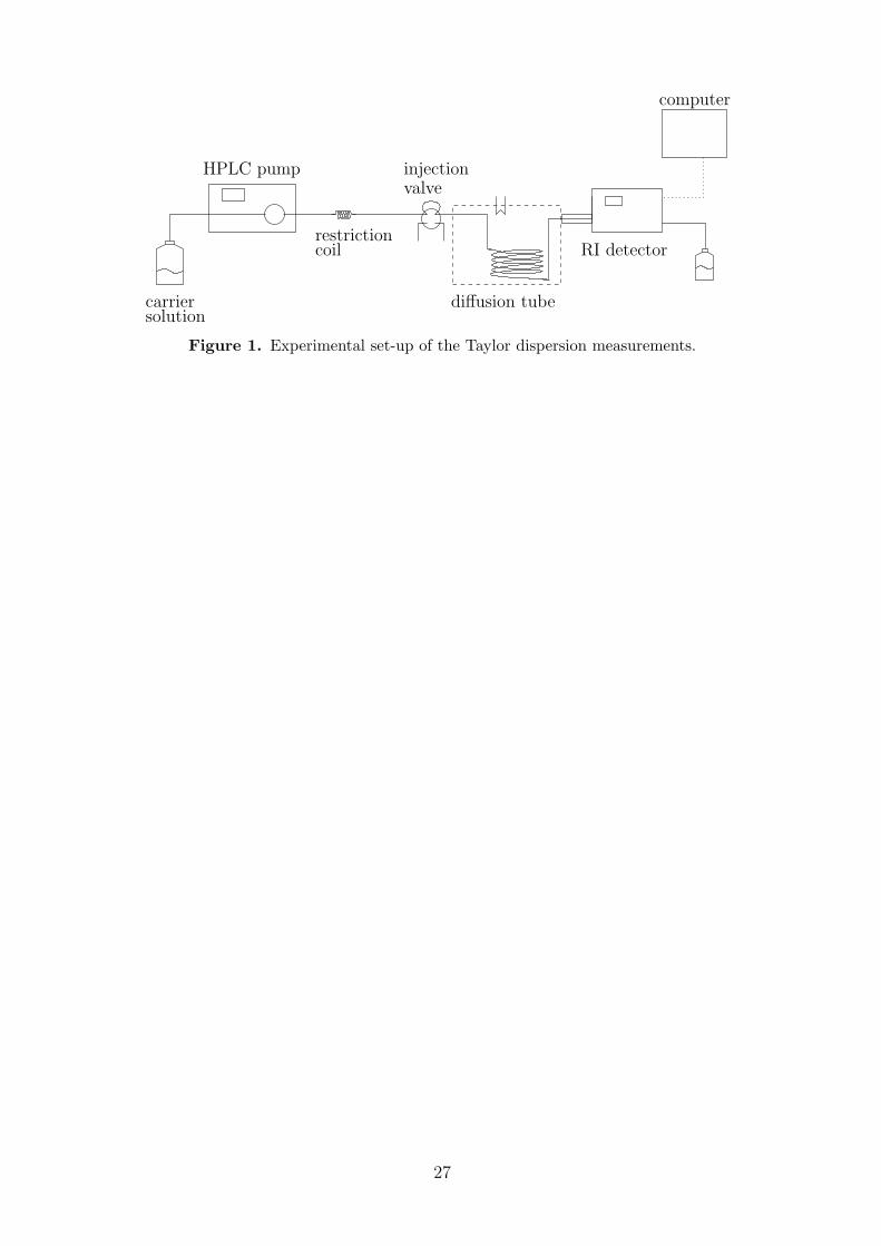
5.1 Apparatus

Figure 1 shows the set-up of the Taylor dispersion equipment that was employed in thiswork. Its design fulfills the criteria described by Alizadeh et al.73. The diffusion tube was apolyetheretherketone (PEEK) capillary with a length L = 30.945 m and an internal diameter2R = 0.53 mm. The capillary was coiled around a cylinder with a radius Rc = 0.2 m andwas placed in a thermostat (Julabo, ± 0.1 K) to maintain a specified temperature. A HPLCpump (Varian ProStar 240) with a built-in pulsation dampener was used to propagate thecarrier solution in laminar flow through the dispersion tube. The part of the dispersion tubebetween the thermostat and the detector was also maintained at the specified temperature byshielding it with insulated tubing through which thermostat water was pumped. Zero deadvolume fittings were used to connect the capillary with a six-port injection valve (Rheodyne7725i) with an injection volume Vinj = 20 µL and with the differential refractive index (RI)detector (Varian ProStart 355 RI). This differential detector measures the difference of therefractive index between the sample stream and a liquid in a reference cell. It is equipped witha thermostatted prism and a low dead volume flow cell (6 µL). The detector was connected toa computer for digital data acquisition using the Galaxy Chromatography Software by Varian.The sampling interval of the detector was 0.2 s.

5.2 Operating Conditions

In order to investigate possible errors arising from pulsation of the HPLC pump, some testruns were carried out with a pulsation-free syringe pump. The Fick diffusion coefficient of themixture water + ethanol at infinite dilution (pure water as a carrier) was measured for thispurpose. The results from three independent measurements obtained with the syringe pumpdeviated by less than 1% from the results with the HPLC pump. Furthermore, no significantdifference with respect to detector noise was observed. This conclusion was also reached byVan de Ven-Lucassen et al.37. Subsequently, the HPLC pump was preferred, because it allowsfor continuous operation.

Taylor’s solution of Eq. (21) requires the composition of the injected sample to be as closeas possible to the composition of the carrier. In this work, the composition difference betweencarrier and injected pulse solution was kept below 0.04 g/g (relative difference). The RIdetector was found to have a linear response up to a mass fraction difference of 0.06 g/g, i.e.the measured diffusion coefficient did not show any significant dependence on the compositionof the pulse solution in this range.

13

The influence of flow rate and capillary tube coiling on the measured Fick diffusion coef-ficient was examined for the two mixtures water + methanol and water + ethanol. Differentexperiments were carried out for flow rates from 0.05 to 0.5 mL min−1. It was found that forflow rates below 0.1 mL min−1, the Fick diffusion coefficient remained constant, whereas itincreased above that flow rate. These erroneously high values of the Fick diffusion coefficientare most likely due to the presence of a secondary flow induced by coiling74. Therefore, anoperating flow rate of 0.05 mL min−1 was chosen. As consequence, the retention time wasbetween 7100 and 7300 s.

5.3 Experimental Procedure

Bidestilled water was used for the present experiments. Both alcohols were of analytical gradeand were purchased from Sigma-Aldrich. Methanol p.a. absolute ≥ 99.8% and Ethanol ACSreagent ≥ 99.5% were used without further purification. The carrier solutions were preparedgravimetrically with an accuracy of ±0.001 g. The pulse solutions were prepared volumet-rically; approximately 10 mL of the carrier solution was poured into a vial, subsequently, asmall amount (0.1 to 0.3 mL) of one of the components was added. After each step, the vialwas weighed to determine the composition of the solution. This procedure was repeated threetimes for each component, giving rise to six different pulse solutions for every measured statepoint. When the carrier was a pure liquid, four different pulse solutions were prepared.

The carrier was allowed to flow through the Taylor apparatus for at least one day to ensurea stationary base line. The pulse solutions were then injected manually into the carrier flow.Every hour after an injection, a new sample was injected into the carrier. The time betweentwo successive injections was chosen such that there was no overlap between the dispersionpeaks of the injected pulses. Each pulse solution was injected at least three times. Hence,a total of 12 (pure carrier) or 18 measurements was carried out for each studied state point.When the carrier solution was exchanged, the apparatus was flushed for 2 h with a flow rateof 1 mL min−1, before it was allowed to run overnight at the operating flow for equilibration.

The detector voltage output signal s(t) was assumed to be linearly dependent on theconcentration change of the flow37. The base line drift of the detector was modeled using apolynomial fit of order N

s(t) = w∆ci +N∑i=0

aiti, (32)

where w is the detector sensitivity. The data acquired by the detector was processed with aMatlab program that was complemented with a visualization tool.

The data processing program employed three different approaches to calculate the Fickdiffusion coefficient from the detector signal. The numerical values of the Fick diffusion co-efficient obtained from these approaches generally differed by less than 0.8%, which is belowthe estimated uncertainty of the Taylor dispersion method.

In the first approach, the baseline was fitted with a cubic polynomial (N = 3) using a leastsquares fit. A visual inspection of the fit was made. If it was not satisfactory, N was increaseduntil a good fit was obtained. The base line drift was then subtracted from the detector signal.In the following step, the program localized and isolated each peak in the detector signal, i.e.data points having values below 5% of a peak maximum were discarded. The data points of an

14

isolated peak were then used to calculate the first and second moments of the concentrationprofile according to Eqs. (25) and (26). The corrections for the first and second moments givenby Alizadeh et al.73 were applied to account for errors caused by a finite injection volume andthe volume of the detector cell. Finally, the Fick diffusion coefficient was calculated with Eq.(27).

The second approach followed the work of Van de Ven-Lucassen et al.37. The followingequation was fitted to the detector signal

s (t) =A√πkt

exp

[−L2 (1− t/τ)2

4kt

]+ a1t+ a0. (33)

Note that the baseline was modeled in this case by a linear function (N = 1). Here, A, k, τ ,a1 and a0 were fitted simultaneously using a trust-region-reflective algorithm75,76.

In the third approach, a three-parameter (A, k and τ) fit was carried out on the basisof data points where the base line was corrected as in case of the first approach. A visualinspection of the validity of the fit was made for every measurement. If the fit was acceptableand the Peclet number was larger than 700, Eq. (24) was employed to calculate the Fickdiffusion coefficient. Otherwise, Eq. (23) was used.

The values for the Fick diffusion coefficient that are obtained with the Taylor dispersionmethod refer to an average composition between the composition of the carrier solution andthat of the injected pulse solution. This effective concentration was calculated by77

ci,eff = ci,car + (ci,inj − ci,car)Vinj2πR3

√48D

πUL· (34)

6 Results

6.1 Experiment

To determine the reliability of the present experimental set-up and the operating procedure,experiments were carried out for the two mixtures water + methanol and water + ethanolat 298.15 K and 1 bar. These mixtures have been studied before by other authors using thediaphragm cell78–82 and the Taylor dispersion technique37,83–86. The present results are givenin Table 2. Each reported value is an average over the individual Fick diffusion coefficientmeasurements of the different injected samples as well as from the three different fitting ap-proaches. The mole fraction is an average over the effective composition calculated by Eq. (34)for each injected solution. The standard deviation of the averaged values is also reported.

The present measurements are consistent with the experimental data from the literaturefor both mixtures at 298.15 K, cf. Figure 2. The average deviation of the present data to apolynomial fit of the literature data sets is in both cases ≤ 2%. Furthermore, the standarddeviation from the observed values was also ≤ 2%, which is in agreement with the expectedaccuracy of the present measurements (2%).

In addition, new experimental data for the Fick diffusion coefficient of the mixture methanol+ ethanol are listed in Table 2 and shown in Figure 2. In this case, the Fick diffusioncoefficient does not exhibit a strong composition dependence, which is in contrast to the

15

aqueous mixtures. The Fick diffusion coefficient depends almost linearly on the mole fraction,which is evidence for an ideal solution. This finding was expected, since both alcohols are verysimilar in terms of their molecular interactions.

Besides the measurements at 298.15 K the isotherm 288.15 K was also considered for themixture water + methanol. To the best of our knowledge, there are no previous measurementsof the Fick diffusion coefficient for this mixture at this temperature. Figure 3 shows the presentresults together with the literature data at 278.15, 298.15 and 308.15 K. It can be seen thatsmall variations of temperature strongly affect the Fick diffusion coefficient, however, thecomposition dependence remains almost unchanged.

The present experimental results are compared with predictions from molecular simulationand classical models in the following section.

6.2 Molecular Simulation

Predictive molecular simulations of transport properties and the thermodynamic factor of theternary mixture water + methanol + ethanol and its binary subsystems were carried out at298.15 K and 1 bar for various compositions as depicted in Figure 4.

The chemical potentials, which were obtained by the gradual insertion method, are listedin Table 3. The ternary Wilson GE model, i.e. Eq. (18) with n = 3, was fitted to thesedata. For this purpose, the binary mixtures were treated as ternary mixtures with a vanishingmole fraction of the absent component. The parameters of the Wilson model are reportedin Table 4. The resulting composition dependence of the chemical potentials is plotted inFigure 5. Figure 6 shows a comparison of the Wilson model with the original simulationdata for the three binary subsystems. While the composition dependence of the chemicalpotentials of the mixture methanol + ethanol is well described by the ideal mixing term lnxi,the aqueous alcohols are strongly non-ideal. A comparison of the Wilson model with trueternary simulation data is given in Table 3. Obviously, the model reproduces the simulationdata well.

On the basis of the Wilson model for the chemical potentials, the thermodynamic fac-tor was computed according to Eq. (19) for the ternary mixture or Eq. (20) for the binarysubsystems. For the latter case, it is compared to the thermodynamic factor obtained fromexperimental VLE data in Figure 7. For this purpose, recommended values for the interactionand non-randomness parameters of the Wilson model were taken (as listed in the DECHEMAVapor-Liquid Equilibrium Data Collection87) for 298.15 K. In addition, the thermodynamicfactor resulting from a direct fit of the Wilson model to experimental VLE data88 at 298.15 Kis plotted. The mole fraction derivatives of the activity coefficients were calculated analyticallyusing the equations given by Taylor and Kooijman10. Figure 7 shows that all three approachesgive a different thermodynamic factor, except for the binary subsystem methanol + ethanol.In particular, the results based on two different parameterizations of the GE model differsubstantially. This demonstrates the general problem encountered when deriving the thermo-dynamic factor from experimental VLE data: although parameterizations of a GE model mayreproduce the VLE data equally well10, the differing composition derivatives may lead to asignificantly differing thermodynamic factor. The fit of the chemical potential to the WilsonGE model, introduces some systematic error to the reported thermodynamic factors. This er-ror was estimated to be less than 5% in magnitude by comparing the thermodynamic factorsreported in this work with the results using other GE models. This shows that the present

16

approach suffers from model sensitivity too, though not as much the classical approach.

Figure 8 shows the MS diffusion coefficient of the three binary subsystems. The presentsimulation results are compared to predictions from the Darken model, Eq. (13). The self-diffusivities needed in the Darken equation were taken from experimental data or were com-puted by EMD simulation. Alternatively, they were predicted with the approach by Liu et al.,Eq. (14), which requires only data at infinite dilution. The most pronounced difference be-tween the data sets is the apparently S-shaped slope of the simulation data for the aqueoussystems, for which the other approaches lead to a convex or concave slope. Except for themixture methanol + ethanol, the Darken model yields only a rough estimate of the MS dif-fusion coefficient, confirming that aqueous alcohols cannot be considered as ideally diffusingmixtures. Similarly, the prediction by Liu et al. fails for the aqueous binaries.

Multiplying the MS diffusion coefficient with the thermodynamic factor according to Eq. (7)leads to the Fick diffusion coefficient. To compare the present method with the method basedon experimental VLE data, the MS diffusion coefficient was multiplied with the thermody-namic factor obtained from present simulations as well as from the VLE approach. In thelatter case, the two parameterizations of the Wilson model were employed as discussed above,resulting in two different values of the thermodynamic factor. Figure 9 compares all respectivesimulation results to the present experimental data.

The present strictly predictive simulation results for the MS and the Fick diffusion coeffi-cients as well as the thermodynamic factor are listed for the binary systems in Table 5. Forthe ternary mixture, the MS diffusion is given in Table 6 in terms of the B−1 matrix, whichis identical to the MS diffusion coefficient in case of binary mixtures, cf. Eqs. (4) and (5).

Figure 9 reveals for the aqueous binary subsystems that the present simulation methodyields a smoother profile for the Fick diffusion coefficient, which qualitatively better reproducesexperimental data than the classical method based on VLE data. Although both methods yieldcomparable deviations from the experimental data points, the profiles resulting from VLE dataare flatter and exhibit a broader minimum, which is most pronounced for the case water +methanol. On the other hand, the simulation results are systematically below the experimentalvalues. An enlarged deviation on the alcohol end of the composition range and a shift of thecomposition minimum are present. These drawbacks are mainly caused by deviations of purecomponent properties. Considering that simple molecular models were used that were fittedto static properties only and the Lorentz-Berthelot combining rule was employed to describethe interaction between unlike LJ sites, the prediction quality with respect to mutual diffusionis nonetheless remarkable.

The simulations of ternary diffusion coefficients yield consistent results. The numericalvalues of D fulfill the theoretical restrictions for thermodynamic stability given by Taylor andKrishna5,i.e. D has positive and real eigenvalues, positive diagonal elements and a positivedeterminant38. The main term diffusion coefficient Dii is larger than Dij, i6=j, which is expectedas the diffusive flow of component i is mainly driven by its own concentration gradient89. Thecoupling effects described by the cross-term diffusion coefficient D21 are usually smaller by oneorder of magnitude than D22. On the other hand, the absolute numerical values of the cross-term diffusion coefficient D12 are important when compared to the main term D22, suggestinglarger coupling effects, which are typical for non-ideal mixtures. With the exception of a singlestate point, the cross-term D12 is negative. Furthermore, D22 is greater than D11 in all cases.

Unfortunately, because of the absence of experimental data on the ternary mixture, it isnot possible to compare them to the present simulation results as it was done for the binary

17

mixtures. However, no dramatic changes in the precision of the present results for ternarymixtures when compared to the binary case are expected. The chemical potential was fittedto a unique model comprising both binary and ternary data and reproduce ternary data asgood as binary ones, thus there is no loss of precision. On the other hand, the simulationuncertainty of the ternary mixtures is expected to be higher but still of the same order ofmagnitude than in the binary case. E.g., the Maxwell-Stefan diffusion coefficients for theternary mixtures contain more terms than the binary ones, so their uncertainty is accordinglyincreased. Another factor that influence the simulation uncertainty is the reduced amount ofparticles for each component in the ternary case because the number of the simulated particleswas kept constant.

To complete the prediction of transport properties, self-diffusion coefficients and shearviscosity are reported in Table 7 and plotted in Figures 10 and 11. The simulation resultsshow a very good agreement with experimental data.

7 Conclusions

The Fick diffusion coefficient of the ternary mixture water + methanol + ethanol was consis-tently determined by equilibrium molecular simulation, i.e. both the MS diffusion coefficientand the thermodynamic factor were calculated by simulation on the basis of a given molecularmodel. The MS diffusion coefficient was sampled by EMD simulation, while the thermo-dynamic factor was obtained from a fit of the Wilson model to the composition profile ofthe chemical potentials that were directly determined by MC simulation. This method wascompared for the studied binary subsystems with the classical method in which the Wilsonmodel is regressed to experimental VLE data. As a benchmark, new experimental data for theFick diffusion coefficient were measured by Taylor dispersion, including the mixture methanol+ ethanol for which no data was previously available. For this almost ideal mixture, bothsimulation methods yielded very similar results and followed the experimental compositiontrend. However, for water + methanol and water + ethanol, the present method predictedthe composition profiles qualitatively better, exhibiting pronounced minima that reflect thestrong non-ideality of these systems. Furthermore, the use of classical method is limited tosystems and conditions for which experimental VLE data exist, and its results vary signifi-cantly depending on which set of VLE data is used. Hence, the present simulation methodis more plausible, while its agreement with experimental results is at least comparable to theclassical method.

Predictive models for the MS diffusion coefficient, i.e. the Darken model and its simplifi-cation by Liu et al., were compared to the present simulation results. For this purpose, theself-diffusion coefficients were simulated. The predictions of these models were found to beunsatisfactory for the aqueous alcohols. To complement the picture of transport properties,the shear viscosity was calculated. Similarly, as in case of the self-diffusion coefficients, theresults for the shear viscosity showed a very good agreement with the experimental data fromthe literature.

When comparing experimental and simulative results, the experiment yields more precisedata for binary mixtures (the accuracy of the Fick diffusion coefficient in present measurementsis 2%). However, the use of experimental techniques for ternary diffusion measurements ishindered by serious complications, leading to the lack of experimental data in the literature.In this case, molecular simulation is an interesting alternative, since the present simulation

18

method does not rely on ternary experimental data and yields the ternary Fick diffusioncoefficient in a similar computation time and with a similar accuracy as in the binary case.

Acknowledgments

The presented research was conducted under the auspices of the Boltzmann-Zuse Society ofComputational Molecular Engineering (BZS), and the simulations were performed on the na-tional supercomputer hermit at the High Performance Computing Center Stuttgart (HLRS)within the project MMHBF2 and on the HP X6000 supercomputer at the Steinbuch Centrefor Computing, Karlsruhe within the project MOCOS. Stanislav Parez acknowledges financialsupport from the ERASMUS Program which enabled his traineeship at University of Pader-born. Finally, we would like to thank Gabor Rutkai for his support in carrying out some ofthe simulation runs.

19

Table 1. Successive states used for the gradual insertion method to couple the fluctuatingmolecule with the system. d∗/d is the geometric factor scaling the intramolecular distances,σ∗/σ as well as ε∗/ε are the fractions of the actual LJ parameters and q∗/q is the fraction ofcharge magnitudes of the fully interacting molecule.

state d∗/d σ∗/σ ε∗/ε q∗/q

0 0 0 0 01 0.10 0.10 0.10 02 0.25 0.25 0.25 03 0.30 0.60 0.60 0.254 0.50 0.90 0.90 0.505 0.75 1.00 1.00 0.756 1 1 1 1

20

Table 2. Fick diffusion coefficient of the binary subsystems containing water (1), methanol(2) or ethanol (3) from present experiment. The numbers in parentheses indicate the standarddeviation in the last digits.

x1 x2 x3 D (288.15 K) D (298.15 K)

molmol−1 molmol−1 molmol−1 10−10m2s−1 10−10m2s−1

water (1) + methanol (2)

0.998 (1) 0.002 (1) 11.87 (14) 15.23 (16)0.800 (1) 0.200 (1) 7.84 (8) 10.31 (10)0.601 (2) 0.399 (2) 7.21 (7) 9.20 (10)0.502 (3) 0.498 (3) 7.69 (12) 10.20 (7)0.401 (2) 0.599 (2) 9.19 (10) 11.83 (14)0.220 (4) 0.780 (4) 12.67 (11) 15.85 (9)0.008 (5) 0.992 (5) 18.29 (10) 21.06 (18)

water (1) + ethanol (3)

0.9990 (8) 0.0010 (8) 12.37 (12)0.899 (2) 0.101 (2) 6.61 (8)0.750 (3) 0.250 (3) 3.83 (6)0.594 (2) 0.406 (2) 4.11 (9)0.506 (3) 0.494 (3) 4.92 (12)0.459 (3) 0.541 (3) 5.54 (11)0.291 (2) 0.709 (2) 7.78 (8)0.189 (4) 0.811 (4) 9.60 (7)0.008 (6) 0.992 (6) 11.65 (10)

methanol (2) + ethanol (3)

0.995 (3) 0.005 (3) 12.32 (10)0.799 (2) 0.201 (2) 13.45 (5)0.601 (2) 0.399 (2) 14.92 (9)0.501 (3) 0.499 (3) 15.60 (6)0.402 (3) 0.598 (3) 16.39 (7)0.201 (3) 0.799 (3) 18.42 (15)0.008 (5) 0.992 (5) 20.34 (18)

21

Table 3. Chemical potentials of the ternary mixture water (1) + methanol (2) + ethanol (3) andits binary subsystems from present simulations. The density ρ was chosen to yield a pressure of1 bar at the temperature 298.15 K. The numbers in parentheses indicate the standard deviationin the last digits. The numbers in square brackets below the ternary data are the correspondingvalues of the present Wilson model.

x1 x2 x3 ρ βµ1 − lnx1 βµ2 − ln x2 βµ3 − lnx3

molmol−1 molmol−1 molmol−1 mol l−1

water (1) + methanol (2)

1.00 0.00 55.29 -12.30 (2)0.95 0.05 52.41 -12.29 (2) -8.18 (11)0.90 0.10 49.80 -12.32 (2) -8.46 (9)0.80 0.20 45.25 -12.27 (3) -8.72 (6)0.60 0.40 37.89 -12.11 (4) -9.13 (5)0.40 0.60 32.33 -11.92 (4) -9.33 (3)0.20 0.80 27.99 -11.73 (5) -9.35 (2)0.10 0.90 26.18 -11.64 (6) -9.34 (2)0.05 0.95 25.31 -11.56 (8) -9.36 (2)0.00 1.00 24.54 -9.34 (4)

water (1) + ethanol (3)

1.00 0.00 55.29 -12.30 (2)0.99 0.01 54.16 -12.30 (2) -7.71 (30)0.90 0.10 46.13 -12.34 (3) -8.64 (21)0.80 0.20 39.33 -12.28 (3) -9.43 (16)0.60 0.40 30.00 -12.10 (3) -9.96 (8)0.40 0.60 24.11 -11.89 (3) -10.04 (5)0.20 0.80 20.08 -11.46 (5) -10.05 (5)0.10 0.90 18.49 -11.34 (6) -10.06 (4)0.01 0.99 17.24 -11.08 (15) -10.10 (2)0.00 1.00 17.13 -10.09 (4)

methanol (2) + ethanol (3)

1.00 0.00 24.54 -9.34 (4)0.89 0.11 23.40 -9.37 (2) -10.09 (7)0.80 0.20 22.57 -9.36 (2) -10.09 (6)0.60 0.40 20.89 -9.35 (2) -10.09 (4)0.40 0.60 19.47 -9.35 (3) -10.07 (4)0.20 0.80 18.21 -9.38 (4) -10.11 (4)0.14 0.86 17.85 -9.39 (4) -10.13 (3)0.00 1.00 17.13 -10.09 (4)

water (1) + methanol (2) + ethanol (3)

0.20 0.40 0.40 23.39 -11.61 (4) -9.42 (2) -10.04 (4)[-11.63] [-9.39] [-10.08]

0.40 0.20 0.40 26.37 -11.83 (3) -9.39 (3) -10.01 (6)[-11.82] [-9.37] [-9.95]

0.40 0.40 0.20 29.045 -11.88 (3) -9.38 (3) -9.99 (5)[-11.88] [-9.32] [-9.93]

0.33 0.33 0.34 26.09 -11.77 (3) -9.37 (2) -9.98 (5)[-11.78] [-9.37] [-9.99]

22

Table 4. Parameters of the Wilson model, cf. Eq. (18), fitted to the chemical potentials of theternary mixture water (1) + methanol (2) + ethanol (3) and its binary subsystems from presentsimulations, cf. Table 3.

M1 -12.34

M2 -9.37

M3 -10.13Λ12 1.02Λ21 0.22Λ13 0.80Λ31 0.10Λ23 1.01Λ32 1.03

23

Table 5. Maxwell-Stefan and Fick diffusion coefficients of the binary subsystems containingwater (1), methanol (2) or ethanol (3) from present simulations. The density ρ was chosen toyield a pressure of 1 bar at the temperature 298.15 K. The numbers in parentheses indicate thestandard deviation in the last digits.

x1 x2 x3 ρ −D Γ D

molmol−1 molmol−1 molmol−1 mol l−1 10−10m2 s−1 10−10m2 s−1

water (1) + methanol (2)

0.95 0.05 52.41 15.5 (1.2) 0.73 11.40.90 0.10 49.80 15.9 (1.1) 0.59 9.40.80 0.20 45.25 17.7 (1.7) 0.48 8.40.70 0.30 41.28 18.0 (1.4) 0.47 8.50.60 0.40 37.89 17.6 (1.9) 0.51 9.00.40 0.60 32.33 16.0 (1.6) 0.65 10.40.20 0.80 27.99 17.0 (1.7) 0.82 13.90.10 0.90 26.18 17.3 (1.7) 0.91 15.70.05 0.95 25.31 17.7 (1.8) 0.95 16.9

water (1) + ethanol (3)

0.99 0.01 54.16 12.2 (7) 0.84 10.30.95 0.05 50.30 10.8 (8) 0.49 5.30.90 0.10 46.13 9.7 (7) 0.32 3.10.80 0.20 39.33 9.7 (8) 0.25 2.40.70 0.30 34.11 11.2 (9) 0.27 3.10.60 0.40 30.00 11.2 (1.0) 0.33 3.70.40 0.60 24.11 10.0 (1.2) 0.51 5.10.20 0.80 20.08 9.5 (1.1) 0.73 7.00.10 0.90 18.49 9.1 (1.1) 0.86 7.830.01 0.99 17.24 10.3 (1.1) 0.99 10.2

methanol (2) + ethanol (3)

0.89 0.11 23.40 21.7 (1.6) 1.01 21.80.80 0.20 22.57 19.5 (2.0) 1.01 19.80.60 0.40 20.89 17.1 (1.9) 1.02 17.50.40 0.60 19.47 16.1 (1.4) 1.02 16.40.20 0.80 18.21 15.0 (1.4) 1.01 15.20.14 0.86 17.85 14.1 (1.4) 1.01 14.2

24

Table 6. Maxwell-Stefan and Fick diffusion coefficients of the ternary mixture water (1) +methanol (2) + ethanol (3) from present simulations. The density ρ was chosen to yield a pressureof 1 bar at the temperature 298.15 K. Note that for the 2×2 matrices B−1, Γ andD, the referencecomponent is ethanol.

x1 x2 x3 ρ B−1 Γ D

molmol−1 molmol−1 molmol−1 mol l−1 10−10m2 s−1 10−10m2 s−1

0.33 0.33 0.34 26.09(

13.4 0.2

−1.7 9.6

) (0.59 −0.10

0.14 1.07

) (8.0 −1.2

0.3 10.5

)0.20 0.40 0.40 23.39

(12.1 −0.1

−0.4 11.7

) (0.75 −0.06

0.06 1.06

) (9.0 −0.9

0.4 12.4

)0.40 0.20 0.40 26.37

(10.0 −1.3

−0.4 11.4

) (0.52 −0.11

0.10 1.06

) (5.1 −2.5

1.0 12.1

)0.40 0.40 0.20 29.05

(12.5 −1.0

−1.6 11.5

) (0.53 −0.12

0.26 1.10

) (6.3 −2.6

2.2 12.9

)0.20 0.20 0.60 21.60

(12.1 0.9

0.3 9.6

) (0.74 −0.06

0.01 1.03

) (8.9 0.2

0.3 9.9

)0.20 0.60 0.20 25.48

(12.9 −1.2

0.7 16.2

) (0.75 −0.06

0.14 1.07

) (9.5 −2.1

2.8 17.2

)0.60 0.20 0.20 33.53

(14.3 −1.8

−3.3 10.1

) (0.34 −0.16

0.27 1.10

) (4.4 −4.3

1.6 11.7

)

25

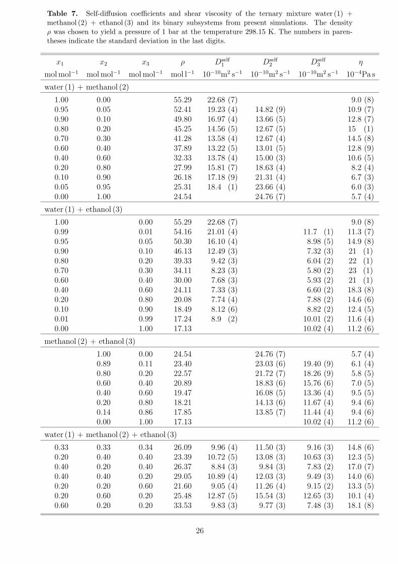
Table 7. Self-diffusion coefficients and shear viscosity of the ternary mixture water (1) +methanol (2) + ethanol (3) and its binary subsystems from present simulations. The densityρ was chosen to yield a pressure of 1 bar at the temperature 298.15 K. The numbers in paren-theses indicate the standard deviation in the last digits.

x1 x2 x3 ρ Dself1 Dself

2 Dself3 η

molmol−1 molmol−1 molmol−1 mol l−1 10−10m2 s−1 10−10m2 s−1 10−10m2 s−1 10−4Pa s

water (1) + methanol (2)

1.00 0.00 55.29 22.68 (7) 9.0 (8)0.95 0.05 52.41 19.23 (4) 14.82 (9) 10.9 (7)0.90 0.10 49.80 16.97 (4) 13.66 (5) 12.8 (7)0.80 0.20 45.25 14.56 (5) 12.67 (5) 15 (1)0.70 0.30 41.28 13.58 (4) 12.67 (4) 14.5 (8)0.60 0.40 37.89 13.22 (5) 13.01 (5) 12.8 (9)0.40 0.60 32.33 13.78 (4) 15.00 (3) 10.6 (5)0.20 0.80 27.99 15.81 (7) 18.63 (4) 8.2 (4)0.10 0.90 26.18 17.18 (9) 21.31 (4) 6.7 (3)0.05 0.95 25.31 18.4 (1) 23.66 (4) 6.0 (3)0.00 1.00 24.54 24.76 (7) 5.7 (4)

water (1) + ethanol (3)

1.00 0.00 55.29 22.68 (7) 9.0 (8)0.99 0.01 54.16 21.01 (4) 11.7 (1) 11.3 (7)0.95 0.05 50.30 16.10 (4) 8.98 (5) 14.9 (8)0.90 0.10 46.13 12.49 (3) 7.32 (3) 21 (1)0.80 0.20 39.33 9.42 (3) 6.04 (2) 22 (1)0.70 0.30 34.11 8.23 (3) 5.80 (2) 23 (1)0.60 0.40 30.00 7.68 (3) 5.93 (2) 21 (1)0.40 0.60 24.11 7.33 (3) 6.60 (2) 18.3 (8)0.20 0.80 20.08 7.74 (4) 7.88 (2) 14.6 (6)0.10 0.90 18.49 8.12 (6) 8.82 (2) 12.4 (5)0.01 0.99 17.24 8.9 (2) 10.01 (2) 11.6 (4)0.00 1.00 17.13 10.02 (4) 11.2 (6)

methanol (2) + ethanol (3)

1.00 0.00 24.54 24.76 (7) 5.7 (4)0.89 0.11 23.40 23.03 (6) 19.40 (9) 6.1 (4)0.80 0.20 22.57 21.72 (7) 18.26 (9) 5.8 (5)0.60 0.40 20.89 18.83 (6) 15.76 (6) 7.0 (5)0.40 0.60 19.47 16.08 (5) 13.36 (4) 9.5 (5)0.20 0.80 18.21 14.13 (6) 11.67 (4) 9.4 (6)0.14 0.86 17.85 13.85 (7) 11.44 (4) 9.4 (6)0.00 1.00 17.13 10.02 (4) 11.2 (6)

water (1) + methanol (2) + ethanol (3)

0.33 0.33 0.34 26.09 9.96 (4) 11.50 (3) 9.16 (3) 14.8 (6)0.20 0.40 0.40 23.39 10.72 (5) 13.08 (3) 10.63 (3) 12.3 (5)0.40 0.20 0.40 26.37 8.84 (3) 9.84 (3) 7.83 (2) 17.0 (7)0.40 0.40 0.20 29.05 10.89 (4) 12.03 (3) 9.49 (3) 14.0 (6)0.20 0.20 0.60 21.60 9.05 (4) 11.26 (4) 9.15 (2) 13.3 (5)0.20 0.60 0.20 25.48 12.87 (5) 15.54 (3) 12.65 (3) 10.1 (4)0.60 0.20 0.20 33.53 9.83 (3) 9.77 (3) 7.48 (3) 18.1 (8)

26

carriersolution

HPLC pump

restrictioncoil

injectionvalve

diffusion tube

RI detector

computer

Figure 1. Experimental set-up of the Taylor dispersion measurements.

27

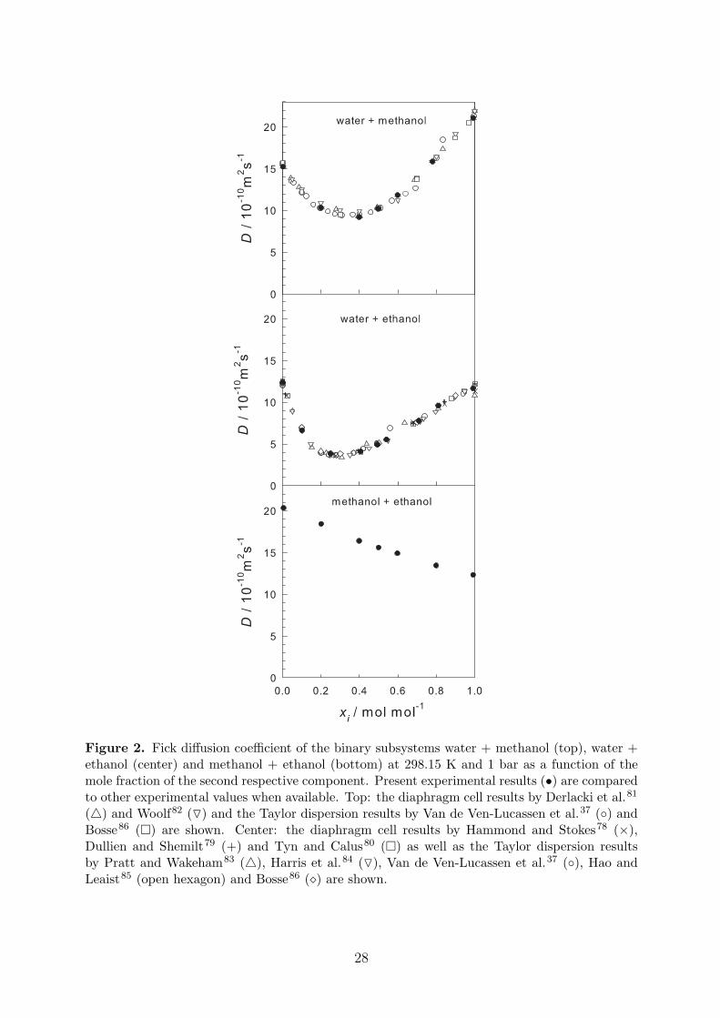
Figure 2. Fick diffusion coefficient of the binary subsystems water + methanol (top), water +ethanol (center) and methanol + ethanol (bottom) at 298.15 K and 1 bar as a function of themole fraction of the second respective component. Present experimental results (•) are comparedto other experimental values when available. Top: the diaphragm cell results by Derlacki et al.81

(4) and Woolf82 (O) and the Taylor dispersion results by Van de Ven-Lucassen et al.37 (◦) andBosse86 (�) are shown. Center: the diaphragm cell results by Hammond and Stokes78 (×),Dullien and Shemilt79 (+) and Tyn and Calus80 (�) as well as the Taylor dispersion resultsby Pratt and Wakeham83 (4), Harris et al.84 (O), Van de Ven-Lucassen et al.37 (◦), Hao andLeaist85 (open hexagon) and Bosse86 (�) are shown.

28

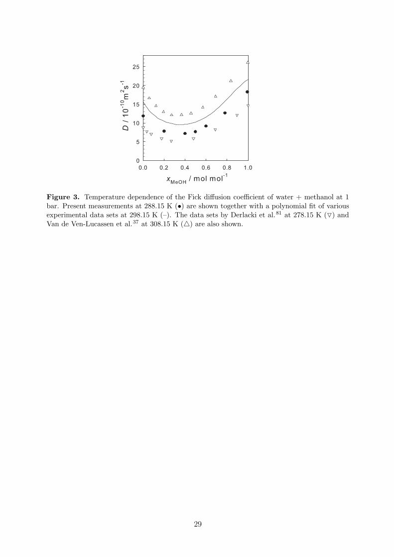
Figure 3. Temperature dependence of the Fick diffusion coefficient of water + methanol at 1bar. Present measurements at 288.15 K (•) are shown together with a polynomial fit of variousexperimental data sets at 298.15 K (–). The data sets by Derlacki et al.81 at 278.15 K (O) andVan de Ven-Lucassen et al.37 at 308.15 K (4) are also shown.

29

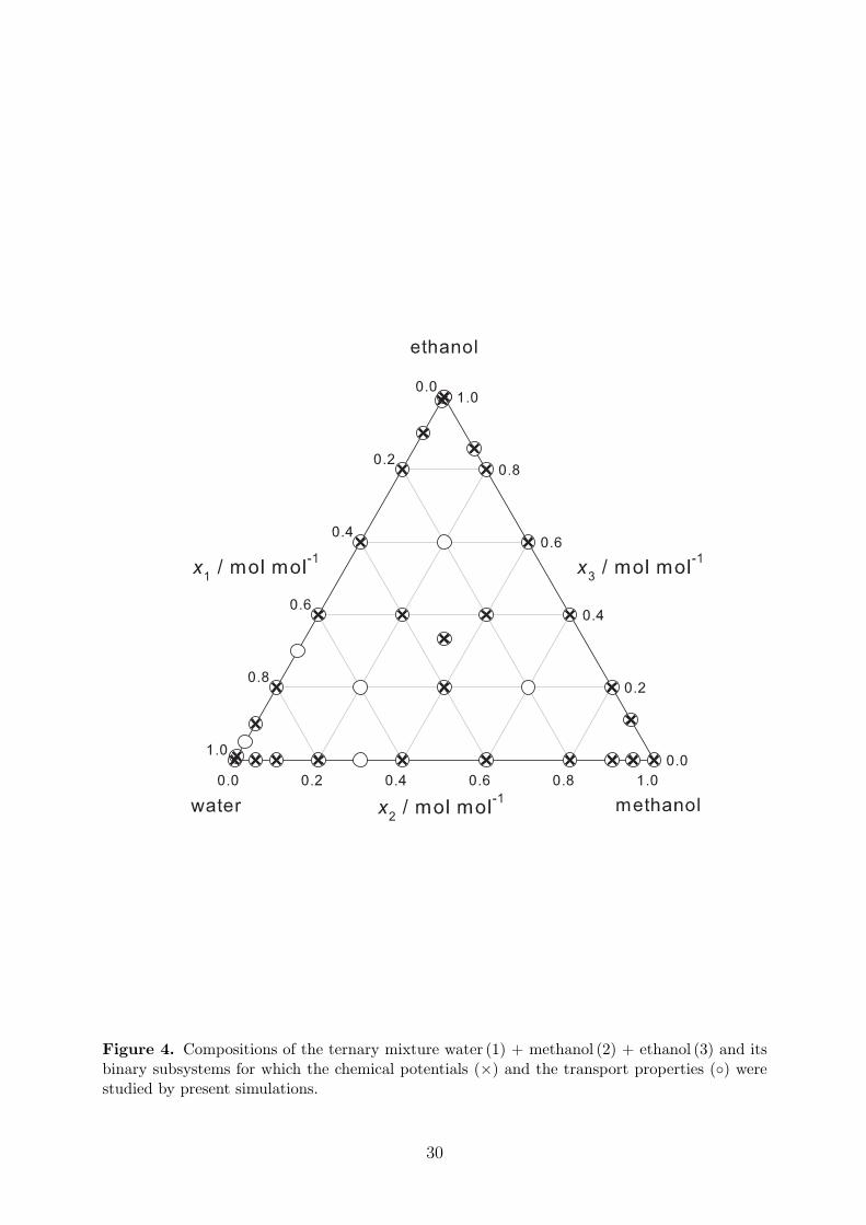
Figure 4. Compositions of the ternary mixture water (1) + methanol (2) + ethanol (3) and itsbinary subsystems for which the chemical potentials (×) and the transport properties (◦) werestudied by present simulations.

30

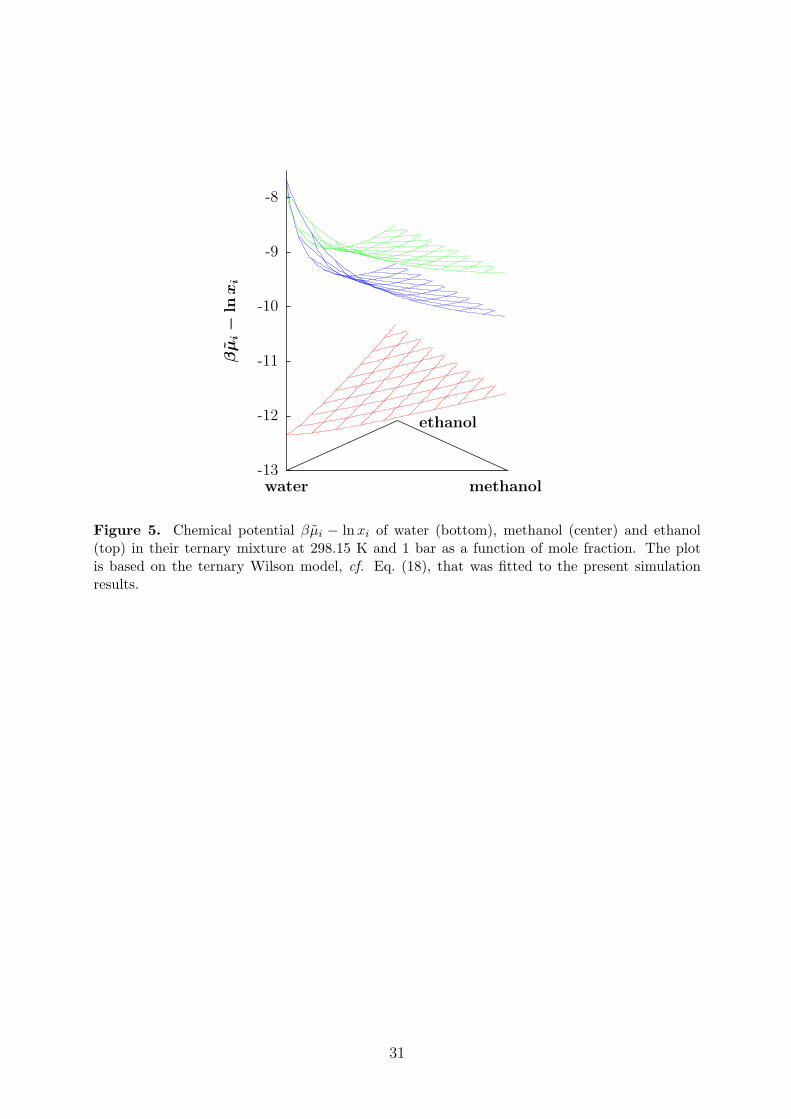
-13

-12

-11

-10

-9

-8

water methanol

ethanol

βµ

i−

lnxi

Figure 5. Chemical potential βµi − lnxi of water (bottom), methanol (center) and ethanol(top) in their ternary mixture at 298.15 K and 1 bar as a function of mole fraction. The plotis based on the ternary Wilson model, cf. Eq. (18), that was fitted to the present simulationresults.

31

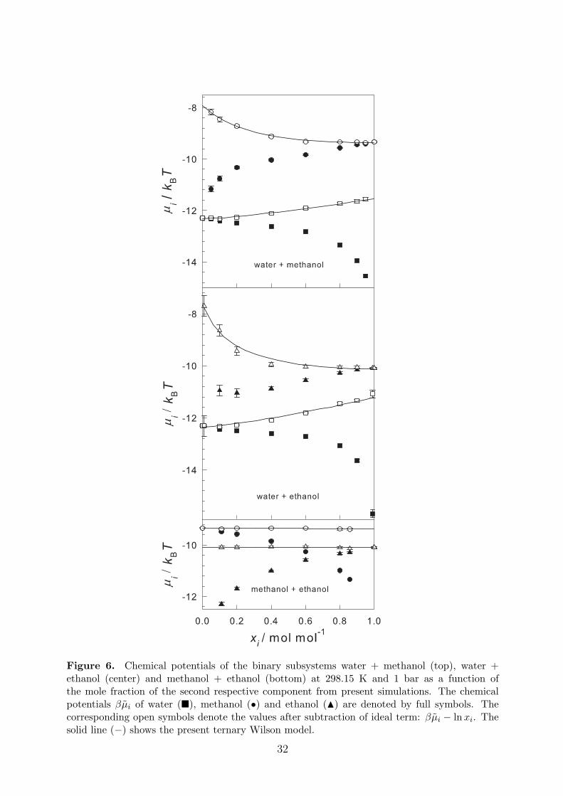
Figure 6. Chemical potentials of the binary subsystems water + methanol (top), water +ethanol (center) and methanol + ethanol (bottom) at 298.15 K and 1 bar as a function ofthe mole fraction of the second respective component from present simulations. The chemicalpotentials βµi of water (�), methanol (•) and ethanol (N) are denoted by full symbols. Thecorresponding open symbols denote the values after subtraction of ideal term: βµi − lnxi. Thesolid line (−) shows the present ternary Wilson model.

32

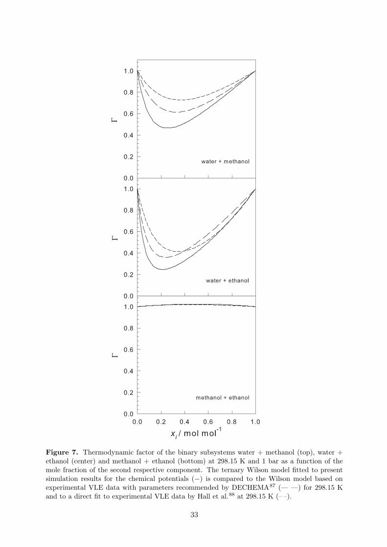
Figure 7. Thermodynamic factor of the binary subsystems water + methanol (top), water +ethanol (center) and methanol + ethanol (bottom) at 298.15 K and 1 bar as a function of themole fraction of the second respective component. The ternary Wilson model fitted to presentsimulation results for the chemical potentials (−) is compared to the Wilson model based onexperimental VLE data with parameters recommended by DECHEMA87 (— —) for 298.15 Kand to a direct fit to experimental VLE data by Hall et al.88 at 298.15 K (– –).

33

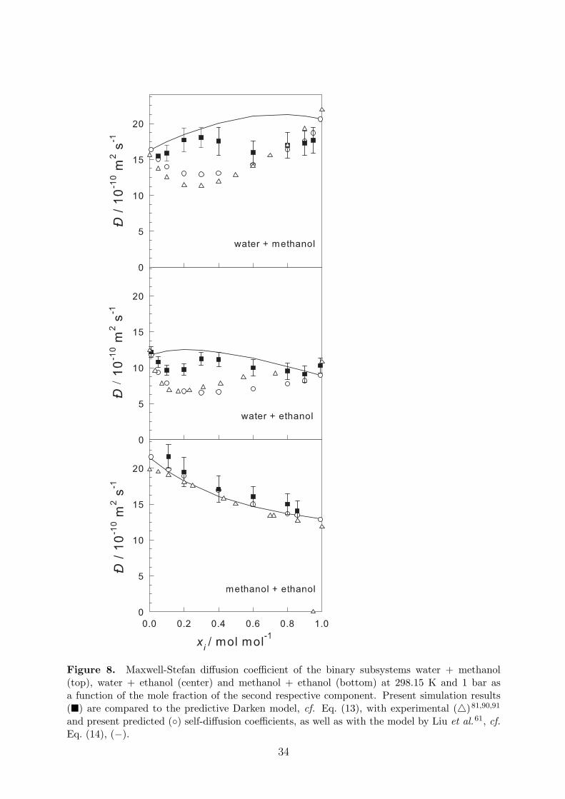
Figure 8. Maxwell-Stefan diffusion coefficient of the binary subsystems water + methanol(top), water + ethanol (center) and methanol + ethanol (bottom) at 298.15 K and 1 bar asa function of the mole fraction of the second respective component. Present simulation results(�) are compared to the predictive Darken model, cf. Eq. (13), with experimental (4)81,90,91

and present predicted (◦) self-diffusion coefficients, as well as with the model by Liu et al.61, cf.Eq. (14), (−).

34

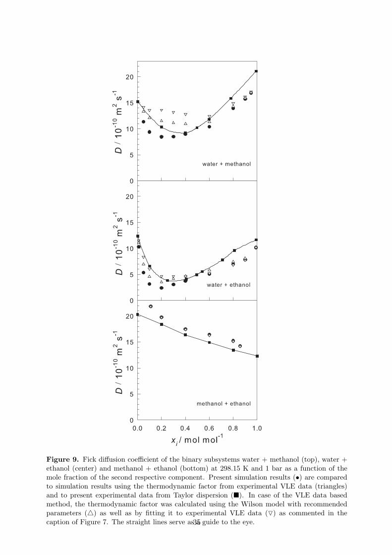
Figure 9. Fick diffusion coefficient of the binary subsystems water + methanol (top), water +ethanol (center) and methanol + ethanol (bottom) at 298.15 K and 1 bar as a function of themole fraction of the second respective component. Present simulation results (•) are comparedto simulation results using the thermodynamic factor from experimental VLE data (triangles)and to present experimental data from Taylor dispersion (�). In case of the VLE data basedmethod, the thermodynamic factor was calculated using the Wilson model with recommendedparameters (4) as well as by fitting it to experimental VLE data (O) as commented in thecaption of Figure 7. The straight lines serve as a guide to the eye.35

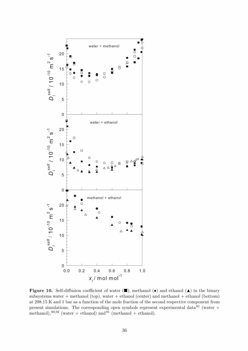
Figure 10. Self-diffusion coefficient of water (�), methanol (•) and ethanol (N) in the binarysubsystems water + methanol (top), water + ethanol (center) and methanol + ethanol (bottom)at 298.15 K and 1 bar as a function of the mole fraction of the second respective component frompresent simulations. The corresponding open symbols represent experimental data81 (water +methanol),90,92 (water + ethanol) and91 (methanol + ethanol).

36

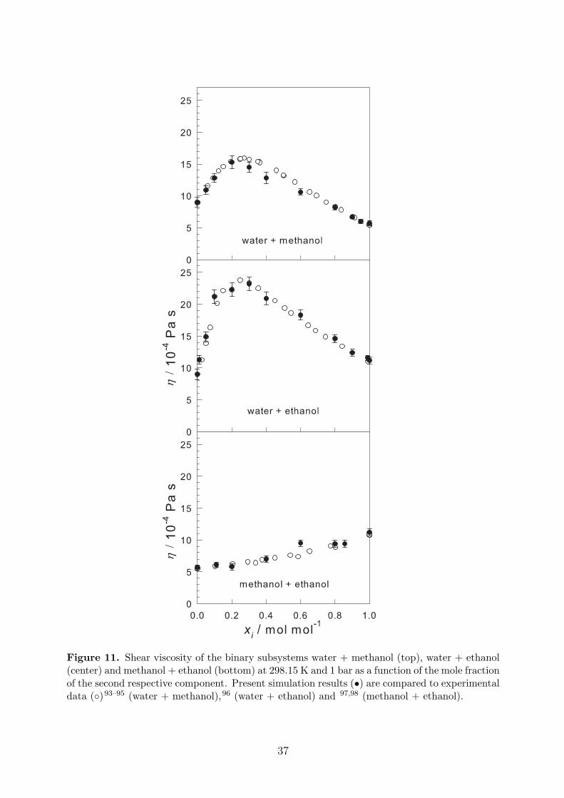
Figure 11. Shear viscosity of the binary subsystems water + methanol (top), water + ethanol(center) and methanol + ethanol (bottom) at 298.15 K and 1 bar as a function of the mole fractionof the second respective component. Present simulation results (•) are compared to experimentaldata (◦)93–95 (water + methanol),96 (water + ethanol) and 97,98 (methanol + ethanol).

37

References

[1] B. Poling, J. Prausnitz and J. O’Connell, The properties of gases and liquids, McGrawHill, New York, 5th edn, 2007.

[2] P. W. M. Rutten, Diffusion in Liquids, Delft University Press, Delft, 1992.

[3] Y. Hu and L. Honglai, Fluid Phase Equilib., 2006, 241, 248.

[4] Y. Hsu and Y. Chen, Fluid Phase Equilib., 1998, 152, 149.

[5] R. Taylor and R. Krishna, Multicomponent mass transfer, John Wiley and sons, NewYork, 1993.

[6] R. Krishna and J. Wesselingh, Chem. Eng. Sci., 1997, 52, 861.

[7] X. Liu, A. Bardow and T. J. H. Vlugt, Ind. Eng. Chem. Res., 2011, 50, 4776.

[8] M. P. Allen and D. J. Tildesley, Computer Simulation of Liquids, Clarendon Press, Ox-ford, 1997.

[9] R. Mills, R. Malhotra, L. A. Woolf and D. G. Miller, J. Chem. Eng. Data, 1994, 39, 929.

[10] R. Taylor and H. Kooijman, Chem. Eng. Comm., 1991, 102, 87.

[11] M. A. Siddiqi and K. Lucas, Can. J. Chem. Eng., 1986, 64, 839.

[12] C. Zhong, Y. Qu and J. He, J. Chem. Eng. Jpn., 2001, 34, 1493.

[13] O. O. Medvedev and A. A. Shapiro, Fluid Phase Equilib., 2003, 208, 291.

[14] D. J. Keffer and P. Adhangale, Chem. Eng. J., 2004, 100, 51.

[15] D. Zabala, C. Nieto-Draghi, J. C. de Hemptinne and A. L. Lopez de Ramos, J. Phys.Chem. B, 2008, 112, 16610.

[16] Z. A. Makrodimitri, D. J. Unruh and I. G. Economou, J. Phys. Chem. B, 2011, 115,1429.

[17] Y. Demirel and H. O. Paksoy, Thermochim. Acta, 1997, 303, 129.

[18] F. A. L. Dullien, Ind. Eng. Chem. Fundam., 1971, 10, 41.

[19] S. Weerasinghe and P. E. Smith, J. Phys. Chem. B, 2005, 109, 15080.

[20] Z. Zhou, B. D. Todd, K. P. Travis and R. J. Sadus, J. Chem. Phys., 2005, 123, 054505.

[21] Y. Kataoka, J. Mol. Liq., 2001, 90, 35.

[22] L. Zhang, Q. Wang, Y.-C. Liu and L.-Z. Zhang, J. Chem. Phys., 2006, 125, 104502.

[23] R. Wedberg, J. P. O’Connell, G. H. Peters and J. Abildskov, Mol. Sim., 2010, 36, 1243.

[24] R. Wedberg, J. P. O’Connell, G. H. Peters and J. Abildskov, J. Chem. Phys., 2011, 135,084113.

38

[25] R. Wedberg, J. P. O’Connell, G. H. Peters and J. Abildskov, Fluid Phase Equilib., 2011,302, 32.

[26] S. K. Schnell, X. Liu, J. M. Simon, A. Bardow, D. Bedeaux, T. J. Vlugt and S. Kjelstrup,J. Phys. Chem. B, 2011, 115, 10911.

[27] S. K. Schnell, T. J. Vlugt, J. M. Simon, D. Bedeaux and S. Kjelstrup, Chem. Phys. Lett.,2011, 504, 199.

[28] S. K. Schnell, T. J. H. Vlugt, J.-M. Simon, D. Bedeaux and S. Kjelstrup, Mol. Phys.,2012, 110, 1069.

[29] T. L. Hill, Thermodynamics of Small Systems, Benjamin, New York, 1963, vol. Part 1.

[30] X. Liu, S. K. Schnell, J.-M. Simon, D. Bedeaux, S. Kjelstrup, A. Bardow and T. J. H.Vlugt, J. Phys. Chem. B, 2011, 115, 12921.

[31] X. Liu, A. Martin-Calvo, E. S. McGarrity, S. K. Schnell, S. Calero, J.-M. Simon, D. Be-deaux, S. Kjelstrup, A. Bardow and T. J. H. Vlugt, Ind. Eng. Chem. Res., 2012, 51,10247.

[32] S. P. Balaji, S. K. Schnell, E. S. McGarrity and T. J. H. Vlugt, Mol. Phys., 2012, doi:10.1080/00268976.2012.720386.

[33] B. Widom, J. Chem. Phys., 1963, 39, 2808.

[34] W. A. Wakeham and M. J. Assael, Chemical thermodynamics for industry, The RoyalSociety of Chemistry, Cambridge, 2004.

[35] G. I. Taylor, Proc. R. Soc. London Ser. A, 1953, 219, 186.

[36] G. I. Taylor, Proc. R. Soc. London Ser. A, 1954, 225, 473.

[37] I. M. J. J. van de Ven-Lucassen, F. G. Kieviet and P. J. A. M. Kerkhof, J. Chem. Eng.Data, 1995, 40, 407.

[38] J. Wambui Mutoru and A. Firoozabadi, J. Chem. Thermodyn., 2011, 43, 1192.

[39] G. Guevara-Carrion, J. Vrabec and H. Hasse, J. Chem. Phys., 2011, 134, 074508.

[40] D. R. Wheeler and R. L. Rowley, Mol. Phys., 1998, 94, 555.

[41] I. M. J. J. van de Ven-Lucassen, T. J. H. Vlugt, A. J. J. van der Zanden and P. J. A. M.Kerkhof, Mol. Simul., 1999, 23, 79.

[42] E. Hawlicka and D. Swiatla-Wojcik, Phys. Chem. Chem. Phys., 2000, 2, 3175.

[43] E. J. W. Wensink, A. Hoffmann, P. J. van Maaren and D. van der Spoel, J. Chem. Phys.,2003, 119, 7308.

[44] F. Muller-Plathe, Mol. Simul., 1996, 18, 133.

[45] S. Y. Noskov, G. Lamoureux and B. Roux, J. Phys. Chem. B, 2005, 109, 6705.

[46] C. Zhang and X. Yang, Fluid Phase Equilib., 2005, 231, 1.

39

[47] G. Guevara-Carrion, C. Nieto-Draghi, J. Vrabec and H. Hasse, J. Phys. Chem. B, 2008,112, 16664.

[48] S. Parez and M. Predota, Phys. Chem. Chem. Phys., 2012, 14, 3640.

[49] M. Predota, P. T. Cummings and D. J. Wesolowski, J. Phys. Chem. C, 2007, 111, 3071.

[50] T. Schnabel, J. Vrabec and H. Hasse, Fluid Phase Equilib., 2005, 233, 134.

[51] T. Schnabel, A. Srivastava, J. Vrabec and H. Hasse, J. Phys. Chem. B, 2007, 111, 9871.

[52] J. L. F. Abascal and C. Vega, J. Chem. Phys., 2005, 123, 234505.

[53] C. Vega and J. L. F. Abascala, Phys. Chem. Chem. Phys., 2011, 13, 19663.

[54] G. S. Fanourgakis, J. S. Medina and R. Prosmiti, J. Phys. Chem. A, 2012, 116, 2564.

[55] S. Tazi, A. Botan, M. Salanne, V. Marry, P. Turq and B. Rotenber, ArXiv:, 2012,1204.2501v1.

[56] M. S. Green, J. Chem. Phys., 1954, 22, 398.

[57] R. Kubo, J. Phys. Soc. Jpn., 1957, 12, 570.

[58] D. J. Keffer, C. Y. Gao and B. J. Edwards, J. Phys. Chem. B, 2005, 109, 5279.

[59] K. E. Gubbins, Statistical Mechanics Vol. 1, The Chemical Society Burlington house,London, 1972.

[60] L. S. Darken, Transactions of the American Institute of Mining and Metallurgical Engi-neers, 1948, 175, 184.

[61] X. Liu, T. J. H. Vlugt and A. Bardow, Ind. Eng. Chem. Res., 2011, 50, 10350.

[62] C. Hoheisel, Phys. Rep., 1994, 245, 111.

[63] M. S. Bello, R. Rezzonico and P. G. Righetti, Science, 1994, 266, 773.

[64] A. M. Bollen, PhD thesis, University of Groningen, 1996.

[65] R. Aris, Proc. R. Soc. London Ser. A, 1956, 235, 67.

[66] H. Flyvbjerg and H. G. Petersen, J. Chem. Phys., 1989, 91, 461.

[67] S. Deublein, J. Vrabec, B. Eckl, J. Stoll, S. V. Lishchuk, G. Guevara-Carrion, C. W. Glass,T. Merker, M. Bernreuther and H. Hasse, Comput. Phys. Comm., 2011, 182, 2350.

[68] M. Schoen and C. Hoheisel, Mol. Phys., 1984, 52, 33.

[69] H. Andersen, J. Chem. Phys., 1980, 72, 2384.

[70] D. Rozmanov and P. G. Kusalik, J. Chem. Phys., 2012, 136, 044507.

[71] K. K. Mon and R. B. Griffiths, Phys. Rev. A, 1985, 31, 956.

[72] I. Nezbeda and J. Kolafa, Mol. Sim., 1991, 5, 391.

40

[73] A. Alizadeh, C. A. Nieto de Castro and W. A. Wakeham, Int. J. Thermophys., 1980, 1,243.

[74] L. A. M. Janssen, Chem. Eng. Sci., 1976, 31, 215.

[75] T. F. Coleman and Y. Li, Mathematical Programming, 1994, 67, 189.

[76] T. F. Coleman and Y. Li, SIAM Journal on Optimization, 1996, 6, 418.

[77] W. Baldauf, PhD thesis, Technical University of Berlin, 1981.

[78] B. R. Hammond and R. H. Stokes, Trans. Farad. Soc., 1953, 49, 890.

[79] F. A. L. Dullien and L. W. Shemilt, Can. J. Chem. Eng., 1961, 39, 242.

[80] M. T. Tyn and W. F. Calus, J. Chem. Eng. Data, 1975, 20, 310.

[81] Z. J. Derlacki, A. J. Easteal, A. V. J. Edge, L. A. Woolf and Z. Roksandic, J. Phys.Chem., 1985, 89, 5318.

[82] L. A. Woolf, Pure & Appl. Chem, 1985, 57, 1083.

[83] K. C. Pratt and W. A. Wakeham, Proc. R. Soc. London Ser. A, 1974, 336, 393.

[84] K. R. Harris, T. Goscinska and H. N. Lam, Chem. Soc., Faraday Trans., 1993, 89, 1969.

[85] L. Hao and D. G. Leaist, J. Chem. Eng. Data, 1996, 41, 210.

[86] D. Bosse, PhD thesis, Technische Universitat Kaiserslautern, 2005.

[87] J. Gmehling, U. Onken and W. Arlt, Vapor-Liquid Equilibrium Data Collection.,DECHEMA, Frankfurt a. M., 2001, vol. 1.

[88] D. J. Hall, C. J. Mash and R. C. Pemberton, NPL Report Chem., 1979, 95, year.

[89] E. L. Cussler,Multicomponent Diffusion, Elsevier Scientific Publishing, Amsterdam, 1976.

[90] K. R. Harris, P. J. Newitt and Z. J. Derlacki, J. Chem. Soc. Faraday Trans., 1998, 94,1963.

[91] P. A. Johnson and A. L. Babb, J. Phys. Chem., 1956, 60, 14.

[92] W. S. Price, H. Ide and Y. Arata, J. Phys. Chem. A, 2003, 107, 4784.

[93] S. Z. Mikhail and W. R. Kimel, J. Chem. Eng. Data, 1961, 6, 533.

[94] J. D. Isdale, A. J. Easteal and L. A. Woolf, Int. J. Thermophys., 1985, 6, 439.

[95] H. Kubota, S. Tsuda, M. Murata, T. Yamamoto, Y. Tanaka and T. Makita, Rev. Phys.Chem. Jpn., 1979, 49, 59.

[96] K. R. Harris and H. N. Lam, J. Chem. Soc. Faraday Trans., 1995, 91, 4071.

[97] I. C. Wei and R. L. Rowley, J. Chem. Eng. Data, 1984, 29, 332.

[98] M. J. Mussche and L. A. Verhoeye, J. Chem. Eng. Data, 1975, 20, 46.

41