Difference-in-Differences with Multiple Time Periods and

an Application on the Minimum Wage and Employment∗

Brantly Callaway† Pedro H. C. Sant’Anna‡

March 24, 2018

Abstract

In this article, we consider identification and estimation of treatment effect parameters

using difference-in-differences (DID) with (i) multiple time periods, (ii) variation in treat-

ment timing, and (iii) when the “parallel trends assumption” holds potentially only after

conditioning on observed covariates. We propose a simple two-step estimation strategy, es-

tablish the asymptotic properties of the proposed estimators, and prove the validity of a

computationally convenient bootstrap procedure. Furthermore we propose a semiparamet-

ric data-driven testing procedure to assess the credibility of the DID design in our context.

Finally, we analyze the effect of the minimum wage on teen employment from 2001-2007.

JEL: C14, C21, C23, J23, J38.

Keywords: Difference-in-Differences, Multiple Periods, Variation in Treatment Timing, Pre-

Testing, Minimum Wage.

∗We thank Andrew Goodman-Bacon, Federico Gutierrez, Na’Ama Shenhav, and seminar participants at the2017 Southern Economics Association for valuable comments. Code to implement the methods proposed in thepaper are available in the R package did which is available on CRAN.†Department of Economics, Temple University. Email: brantly.callaway@temple.edu‡Department of Economics, Vanderbilt University. Email: pedro.h.santanna@vanderbilt.edu

1

1 Introduction

Difference-in-Differences (DID) has become one of the most popular designs used to evaluate the

causal effect of policy interventions. In its canonical format, there are two time periods and

two groups: in the first period, no one is treated and in the second period some individuals are

treated (the treated group) and some individuals are not (the control group). If, in the absence

of treatment, the average outcomes for treated and control groups would have followed parallel

paths over time (which is the so-called parallel trends assumption), one can measure the average

treatment effect for the treated subpopulation (ATT) by comparing the average change in outcomes

experienced by the treated group to the average change in outcomes experienced by the control

group. Most methodological extensions of DID methods have been confined to this standard two

periods, two groups setup, see e.g. Heckman et al. (1997, 1998), Abadie (2005), Athey and Imbens

(2006), Qin and Zhang (2008), Bonhomme and Sauder (2011), de Chaisemartin and D’Haultfœuille

(2017), Botosaru and Gutierrez (2017), and Callaway et al. (2018).

Many DID empirical applications, however, deviate from the standard DID setup. For example,

half of the articles published in 2014/2015 in the American Economic Review, Quarterly Journal

of Economics, and the Journal of Political Economy that used DID methods had more than two

time periods and exploited variation in treatment timing.1 In these cases, researchers usually

consider the following regression model

Yit = αt + ci + βDit + θXi + εit,

where Yit is the outcome of interest, αt is a time fixed effect, ci is an individual/group fixed

effect, Dit is a treatment indicator that takes value one if an individual i is treated at time

t and zero otherwise, Xi is a vector of observed characteristics, and εit is an error term, and

interpret β as the causal effect of interest. Despite the popularity of this approach, Wooldridge

(2005), Chernozhukov et al. (2013), de Chaisemartin and D’Haultfoeuille (2016), Borusyak and

Jaravel (2017), Goodman-Bacon (2017) and S loczynski (2017) have shown that once one allows

for heterogeneous treatment effects, β does not represent an easy to interpret average treatment

1We thank Andrew Goodman-Bacon for sharing with us this statistic.

2

effect parameter. As a consequence, inference about the effectiveness of a given policy can be

misleading when based on such a two-way fixed effects regression model.

In this article we aim to fill this important gap and consider identification and inference proce-

dures for average treatment effects in DID models with (i) multiple time periods, (ii) variation in

treatment timing, and (iii) when the parallel trends assumption holds potentially only after con-

ditioning on observed covariates. First, we provide conditions under which the average treatment

effect for group g at time t is nonparametrically identified, where a “group” is defined by when

units are first treated. We call these causal parameters group-time average treatment effects.

Second, although these disaggregated group-time average treatment effects can be of interest

by themselves, in some applications there are perhaps too many of them, potentially making the

analysis of the effectiveness of the policy intervention harder, particularly when the sample size

is moderate. In such cases, researchers may be interested in summarizing these disaggregated

causal effects into a single, easy to interpret, causal parameter. We suggest different ideas for

combining the group-time average treatment effects, depending on whether one allows for (a)

selective treatment timing, i.e., allowing, for example, the possibility that individuals with the

largest benefits from participating in a treatment choose to become treated earlier than those

with a smaller benefit; (b) dynamic treatment effects – where the effect of a treatment can depend

on the length of exposure to the treatment; or (c) calendar time effects – where the effect of

treatment may depend on the time period. Overall, we note that the best way to aggregate the

group-time average treatment effects is likely to be application specific. Aggregating group-time

parameters is also likely to increase statistical power.

Third, we develop the asymptotic properties for a semiparametric two-step estimator for the

group-time average treatment effects, and for the different aggregated causal parameters. Estimat-

ing these treatment effects involves estimating a generalized propensity score for each group g, and

using these to construct appropriate weights for a “long difference” of outcomes. We establish√n-

consistency and asymptotic normality of our estimators. We propose computationally convenient

bootstrapped simultaneous confidence bands that can be used for visualizing estimation uncer-

tainty for the group-time average treatment effects. Unlike traditional pointwise confidence bands,

3

our simultaneous confidence bands asymptotically cover the entire path of the group-time average

treatment effects with probability 1−α. Importantly, our inference procedures can accommodate

clustering in a relatively straightforward manner.

Finally, it is important to emphasize that all the aforementioned results rely on the fundamen-

tally untestable conditional parallel trends assumption. Nonetheless, we note that if one imposes a

slightly stronger conditional parallel trends assumption – namely, that conditional parallel trends

holds in all periods, specifically including pre-treatment periods – there are testable implications,

provided the availability of more than two time periods. A fourth contribution of this article is to

take advantage of this observation and propose a falsification test based on it. Our pre-test for

the plausibility of the conditional parallel trends assumption is based on the integrated moments

approach, see e.g. Bierens (1982) and Stute (1997), completely avoids selecting tuning parame-

ters, and is fully data-driven. We use results from the empirical processes literature to study the

asymptotic properties of our falsification test. In particular, we derive its asymptotic null distri-

bution, prove that it is consistent against fixed nonparametric alternatives, and show that critical

values can be computed with the assistance of an easy to implement multiplier-type bootstrap.

We illustrate the appeal of our method by revisiting findings about the effect of the minimum

wage on teen employment. Although standard economic theory says that a wage floor should

result in lower employment, there is a bulk of literature that finds no disemployment effects of the

minimum wage, even when focusing on groups that are most likely to be affected by minimum

wage increases such as teenagers or fast-food restaurant employees. Notable among these is the

landmark DID paper, Card and Krueger (1994), Dube et al. (2010), among many others; see also

Doucouliagos and Stanley (2009), Schmitt (2013), and Belman and Wolfso (2014) for summaries

of the literature. There is notable disagreement with this view though. For instance, in a series of

work, David Neumark and William Wascher (see e.g. Neumark and Wascher (1992, 2000, 2008),

Neumark et al. (2014)), as well as Jardim et al. (2017) provide evidence for the view that increasing

the minimum wage decreases employment.

We use data from 2001-2007, where the federal minimum wage was flat at $5.15 per hour.

Using a period where the federal minimum wage is flat allows for a clear source of identification

4

- state level changes in minimum wage policy. However, we also need to confront the issue that

states changed their minimum wage policy at different points in time over this period – an issue

not encountered in the case study approach to studying the employment effects of the minimum

wage. In addition, for states that changed their minimum wage policy in later periods, we can

pre-test the parallel trends assumption which serves as a check of the internal consistency of the

models used to identify minimum wage effects.

We consider both an unconditional and conditional DID approach to estimating the effect of

increasing the minimum wage on teen employment rates. For the unconditional case, we find that

increases in the minimum wage tend to decrease teen employment; the effects range from 2.3%

lower teen employment to 13.6% lower teen employment across groups and time. This result is not

surprising; most of the work on the minimum wage that reaches a similar conclusion uses a similar

setup. Dube et al. (2010) points out that such negative effects may be spurious given potential

violations of the common trend assumption. Indeed, when we tests for the reliability of the

unconditional common trend assumption, we reject it. Given that we reject the unconditional DID

design, we then follow Dube et al. (2010) proposal and consider a two-way fixed effects regression

model with region-year fixed effects. As in Dube et al. (2010), such an estimation strategy finds no

adverse effect on teen employment. Nonetheless, one must bear in mind that, as discussed before,

such two-way fixed effects regressions may not identify easy to interpret causal parameters. To

circumvent this issue, we use our conditional DID approach and find that increasing the minimum

wage does tend to decrease teen employment with effects ranging from 0.8% higher employment

(not statistically significant) to 7.3% lower employment across groups and time. In addition, like

Meer and West (2016), we find that the effect of minimum wage increases is dynamic – the effect

is increasing in the length of exposure to the minimum wage increase. However, we find evidence

against the conditional parallel trends assumption using our pre-test. Thus, our findings should

be interpreted with care.

The methodological results in this article are related to other papers in the DID literature.

Heckman et al. (1997, 1998), Blundell et al. (2004), Abadie (2005), and, Qin and Zhang (2008)

consider identifying assumptions similar to ours, but focus on the standard DID setup of two

5

periods, two groups. Our proposal particularly builds on Abadie (2005) as we also adjusts for

covariates using propensity score weighting. On top of accounting for variation in treatment

timing, another important difference between our proposal and Abadie (2005) is that our estimator

is based on stabilized (normalized) weights, whereas his proposed estimator is of the Horvitz and

Thompson (1952) type. As the simulations results in Busso et al. (2014) show, stabilized weights

can lead to important finite sample improvements when compared to Horvitz and Thompson

(1952) type estimators.

Our pre-test for the plausibility of the conditional parallel trends assumption is also related

to many papers in the goodness-of-fit literature, including Bierens (1982), Bierens and Ploberger

(1997), Stute (1997), Stinchcombe and White (1998), Escanciano (2006a,b, 2008), Sant’Anna

(2017), and Sant’Anna and Song (2018); for a recent overview, see Gonzalez-Manteiga and Cru-

jeiras (2013). Despite the similarities, we seem to be the first to realize that such a procedure could

be used to pre-test for the reliability of the conditional parallel trends identification assumption.

The remainder of this article is organized as follows. Section 2 presents our main identification

results. We discuss estimation and inference procedures for the treatment effects of interest in

Section 3. Section 4 describes our pre-tests for the credibility of the conditional parallel trends

assumption. We revisit the effect of minimum wage on employment in Section 5. Section 6

concludes. All proofs are gathered in the Appendix.

2 Identification

2.1 Framework

We first introduce the notation we use throughout the article. We consider the case with T periods

and denote a particular time period by t where t = 1, . . . , T . In a standard DID setup, T = 2 and

no one is treated in period 1. Let Dt be a binary variable equal to one if an individual is treated in

period t and equal to zero otherwise. Also, define Gg to be a binary variable that is equal to one

if an individual is first treated in period g, and define C as a binary variable that is equal to one

for individuals in the control group – these are individuals who are never treated so the notation

6

is not indexed by time. For each individual, exactly one of the Gg or C is equal to one. Denote

the generalized propensity score as pg(X) = P (Gg = 1|X,Gg +C = 1). Note that pg(X) indicates

the probability that an individual is treated conditional on having covariates X and conditional

on being a member of group g or the control group. Finally, let Yt (1) and Yt (0) be the potential

outcome at time t with and without treatment, respectively. The observed outcome in each period

can be expressed as Yt = DtYt (1) + (1−Dt)Yt (0) .

Given that Yt (1) and Yt (0) cannot be observed for the same individual at the same time,

researchers often focus on estimating some function of the potential outcomes. For instance, in

the standard DID setup, the most popular treatment effect parameter is the average treatment

effect on the treated, denoted by2

ATT = E[Y2(1)− Y2(0)|G2 = 1].

Unlike the two period and two group case, when there are more than two periods and variation

in treatment timing, it is not obvious which is the main causal parameter of interest. Instead, we

consider the the average treatment effect for individuals first treated in period g at time period t,

denoted by

ATT (g, t) = E[Yt(1)− Yt(0)|Gg = 1].

We call this causal parameter the group-time average treatment effect. In particular, note that in

the classical DID setup, ATT (2, 2) collapses to ATT .

In this article, we are interested in identifying and estimating ATT (g, t) and functions of

ATT (g, t). Towards this end, we impose the following assumptions.

Assumption 1 (Sampling). {Yi1, Yi2, . . . YiT , Xi, Di1, Di2, . . . , DiT }ni=1 is independent and identi-

cally distributed (iid).

Assumption 2 (Conditional Parallel Trends). For all t = 2, . . . , T , g = 2, . . . , T such that g ≤ t,

E[Yt(0)− Yt−1(0)|X,Gg = 1] = E[Yt(0)− Yt−1(0)|X,C = 1] a.s..

2Existence of expectations is assumed throughout.

7

Assumption 3 (Irreversibility of Treatment). For t = 2, . . . , T ,

Dt = 1 implies that Dt+1 = 1

Assumption 4 (Overlap). For all g = 2, . . . , T , P (Gg = 1) > 0 and pg(X) < 1 a.s..

Assumption 1 implies that we are considering the case with panel data. The extension to

the case with repeated cross sections is relatively simple and is developed in Appendix B in the

Supplementary Appendix.

Assumption 2, which we refer to as the (conditional) parallel trends assumption throughout the

paper, is the crucial identifying restriction for our DID model, and it generalizes the two-period

DID assumption to the case where it holds in all periods and for all groups; see e.g. Heckman et al.

(1997, 1998), Blundell et al. (2004), and Abadie (2005). It states that, conditional on covariates,

the average outcomes for the group first treated in period g and for the control group would

have followed parallel paths in the absence of treatment. We require this assumption to hold for

all groups g and all time periods t such that g ≤ t; that is, it holds in all periods after group

g is first treated. It is important to emphasize that the parallel trends assumption holds only

after conditioning on some covariates X, therefore allowing for X-specific time trends. All of our

analysis continues to go through in the case where an unconditional parallel trends assumption

holds by simply setting X = 1.

Assumption 3 states that once an individual becomes treated, that individual will also be

treated in the next period. With regards to the minimum wage application, Assumption 3 says

that once a state increases its minimum wage above the federal level, it does not decrease it back

to the federal level during the analyzed period. Moreover, this assumption is consistent with most

DID setups that exploit the enacting of a policy in some location while the policy is not enacted

in another location.3

Finally, Assumption 4 states that a positive fraction of the population started to be treated in

period g, and that, for any possible value of the covariates X, there is some positive probability

3One could potentially relax this assumption by forming groups on the basis of having the entire path oftreatment status being the same and then perform the same analysis that we do.

8

that an individual is not treated.4 This is a standard covariate overlap condition, see e.g. Heckman

et al. (1997, 1998), Blundell et al. (2004), Abadie (2005).

Remark 1. In some applications, eventually all units are treated, implying that C is never equal

to one. In such cases one can consider the “not yet treated” (Dt = 0) as a control group instead of

the “never treated” (C = 1). We consider this case in Appendix C in the Supplementary Appendix,

which resembles the event study research design, see e.g. Borusyak and Jaravel (2017).

2.2 Group-Time Average Treatment Effects

In this section, we introduce the nonparametric identification strategy for the group-time average

treatment effect ATT (g, t). Importantly, we allow for arbitrary treatment effect heterogeneity.

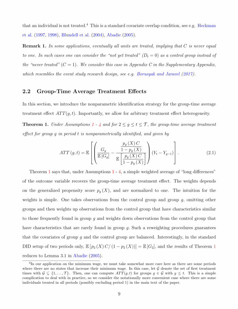
Theorem 1. Under Assumptions 1 - 4 and for 2 ≤ g ≤ t ≤ T , the group-time average treatment

effect for group g in period t is nonparametrically identified, and given by

ATT (g, t) = E

Gg

E [Gg]−

pg (X)C

1− pg (X)

E[pg (X)C

1− pg (X)

] (Yt − Yg−1)

. (2.1)

Theorem 1 says that, under Assumptions 1 - 4, a simple weighted average of “long differences”

of the outcome variable recovers the group-time average treatment effect. The weights depends

on the generalized propensity score pg (X), and are normalized to one. The intuition for the

weights is simple. One takes observations from the control group and group g, omitting other

groups and then weights up observations from the control group that have characteristics similar

to those frequently found in group g and weights down observations from the control group that

have characteristics that are rarely found in group g. Such a reweighting procedures guarantees

that the covariates of group g and the control group are balanced. Interestingly, in the standard

DID setup of two periods only, E [p2 (X)C/ (1− p2 (X))] = E [G2], and the results of Theorem 1

reduces to Lemma 3.1 in Abadie (2005).

4In our application on the minimum wage, we must take somewhat more care here as there are some periodswhere there are no states that increase their minimum wage. In this case, let G denote the set of first treatmenttimes with G ⊆ {1, . . . , T }. Then, one can compute ATT (g, t) for groups g ∈ G with g ≤ t. This is a simplecomplication to deal with in practice, so we consider the notationally more convenient case where there are someindividuals treated in all periods (possibly excluding period 1) in the main text of the paper.

9

To shed light on the role of the “long difference”, we give a sketch of how this argument works

in the unconditional case, i.e., when X = 1. Recall that the key identification challenge is for

E[Yt(0)|Gg = 1] which is not observed when g ≤ t. Under the parallel trends assumption,

E[Yt(0)|Gg = 1] = E[Yt(0)− Yt−1(0)|Gg = 1] + E[Yt−1(0)|Gg = 1]

= E[Yt − Yt−1|C = 1] + E[Yt−1(0)|Gg = 1]

The first term is identified, it is the change in outcomes between t − 1 and t experienced by the

control group. If g > t− 1, then the last term is identified. If not,

E[Yt−1(0)|Gg = 1] = E[Yt−1 − Yt−2|C = 1] + E[Yt−2(0)|Gg = 1]

which holds under the parallel trends assumption. If g > t−2, then every term above is identified.

If not, one can proceed recursively in this same fashion until

E[Yt(0)|Gg = 1] = E[Yt − Yg−1|C = 1] + E[Yg−1|Gg = 1],

implying the result for ATT (g, t).

One final thing to consider in this section is the case when the parallel trends assumption holds

without needing to condition on covariates. In this case, (2.1) simplifies to

ATT (g, t) = E[Yt − Yg−1|Gg = 1]− E[Yt − Yg−1|C = 1], (2.2)

which is simpler than the weighted representation in (2.1) but also implies that all of our results will

also cover the unconditional case which is very commonly used in empirical work. We discuss an

alternative regression based approach to obtaining ATT (g, t) in Appendix D in the Supplementary

Appendix.5

5Unlike the two period, two group case, there does not appear to be any advantage to trying to obtain ATT (g, t)from a regression as it appears to require post-processing the regression output.

10

2.3 Summarizing Group-time Average Treatment Effects

The previous section shows that the group-time average treatment effect ATT (g, t) is identified for

g ≤ t. These are very useful parameters – they allow one to consider how the effect of treatment

varies by group and time. However, in some applications there may be many of them, perhaps

too many to easily interpret the effect of a given policy intervention. This section considers ways

to aggregate group-time average treatment effects into a few number of interpretable causal effect

parameters. In applications, aggregating the group-time average treatment effects is also likely to

increase statistical power, reducing estimation uncertainty.

The two simplest ways of combining ATT (g, t) across g and t are

2

T (T − 1)

T∑g=2

T∑t=2

1{g ≤ t}ATT (g, t) and1

κ

T∑g=2

T∑t=2

1{g ≤ t}ATT (g, t)P (G = g) (2.3)

where κ =∑T

g=2

∑Tt=2 1{g ≤ t}P (G = g) (which ensures that the weights on ATT (g, t) in the

second term sum to 1).6 The first term in (2.3) is just the simple average of ATT (g, t); the second

is a weighted average of each ATT (g, t) putting more weight on ATT (g, t) with larger group sizes.

As we argue below, neither of the terms in (2.3) are likely to be “appropriate” summary treatment

effect measures, except in the particular case where the effect of treatment is homogeneous across

groups and time.

In contrast to our approach in this section, the most common approach to estimating the effect

of a binary treatment in a panel data setup is to interpret β in the following regression as the

average treatment effect

Yit = αt + ci + βDit + θXi + εit,

where αt is a time fixed effect and ci is an individual/group fixed effect. Interestingly, Wooldridge

(2005), Chernozhukov et al. (2013), de Chaisemartin and D’Haultfoeuille (2016), Borusyak and

Jaravel (2017), Goodman-Bacon (2017) and S loczynski (2017) have shown that, in general, β does

not represent an easy to interpret average treatment effect parameter. The results in this section

6Here we use the shorthand notation P (G = g) to denote P (Gg = 1|G1 + C = 0) . Thus, P (G = g) is theprobability that an individual is first treated in period g conditional on not being in the control group or in thegroup first treated in period 1. Throughout this section, conditional probabilities such as P (G = g|g ≤ t) alsoimplicitly condition on not being in the control group or in the group first treated in period 1.

11

can be used in exactly the same setup to identify a single interpretable average treatment effect

parameter and, thus, provide a way to circumvent the issues with the more common approach.

In the following, we consider several common cases that are likely to occur in practice: (a)

selective treatment timing, (b) dynamic treatment effects, and (c) calendar time effects. We

provide some recommendations on constructing interpretable treatment effect parameters under

each of these setups. It is worth mentioning that in each of these cases, ATT (g, t) still provides

the average causal effect of the treatment for group g in period t; the issue in this section is how

to aggregate ATT (g, t) into a smaller number of causal effect parameters.

Selective Treatment Timing In many cases, when to become treated is a choice variable.

The parallel trends assumptions does place some restrictions on how individuals select when to be

treated. In particular, in order for the path of untreated potential outcomes to be the same for a

particular group and the control group, the parallel trends assumption does not permit individuals

to select into treatment in period t because they anticipate Yt(0) being small (assuming larger Y

is “good”). On the other hand, the parallel trends assumption does not place restrictions on how

treated potential outcomes are generated. Thus, our imposed DID assumptions fully allow for

individuals to select into treatment on the basis of expected future values of treated potential

outcomes.

While some forms of selective treatment timing are permitted under the parallel trends as-

sumption and do not affect identification of group-time average treatment effects, they do have

implications for the “best ways” to combine ATT (g, t) into a single, easy to interpret treatment

effect parameter. In particular, when there is selective treatment timing, the period when an

individual is first treated may provide information about the size of the treatment effect. In such

cases, we propose to summarize the causal effect of a policy by first aggregating ATT (g, t) by

group, and then combine group average treatment effects based on the size of each group.

More precisely, we first consider

θS(g) =1

T − g + 1

T∑t=2

1{g ≤ t}ATT (g, t).

12

Note that θS(g) is the time-averaged treatment effect for individuals in group g, i.e., just a time-

average of each available ATT (g, t) for group g. Next, in order to further reduce the dimensionality

of θS(g), one can average θS(g) across groups to get

θS =T∑g=2

θS(g)P (G = g). (2.4)

Note that θS appears to be quite similar to the second term in (2.3). The difference is in the

weights. The second term in (2.3) puts more weight on groups that are exposed to treatment

longer. The weights in (2.4) only depend on group size, not on the number of post-treatment

periods available per group. For example, suppose there is positive selective treatment timing so

that individuals who are treated earlier experience larger benefits from being treated than those

who are treated later. In the presence of selective treatment timing, the approach in (2.3) would

tend to overstate the effect of the treatment due to putting more weight on the groups that are

treated the longest, which are precisely the ones that experience the largest benefits of being

treated. Thus, we argue that, in the presence of selective treatment timing, θS in (2.4) is a more

natural causal parameter than the second term in (2.3).

Dynamic Treatment Effects In other cases, the effect of a policy intervention may depend on

the length of exposure to it. To give some examples, Jacobson et al. (1993) argues that workers

that are displaced from their jobs tend to have immediate large earnings effects that get smaller

over time, and both the immediate effect and the dynamic effect are of interest. In the case of the

minimum wage, Meer and West (2016) argue that increasing the minimum wage leads to lower job

creation and thus that the effect of the minimum wage on employment is dynamic – one should

expect larger effects in subsequent periods than in the initial period.

In the presence of dynamic treatment effects (but not selective treatment timing), we propose

to summarize the effects of the policy by first aggregating ATT (g, t) by the length of exposure to

treatment (we denote this by e), and then (possibly) combining average effects based on length of

13

exposure by averaging over different lengths of exposure. That is, we first consider the parameter

θD(e) =T∑g=2

T∑t=2

1{t− g + 1 = e}ATT (g, t)P (G = g|t− g + 1 = e),

which provides the average effect of treatment for individuals that have been treated for exactly e

periods. For example, when e = 1, it averages (based on group size) ATT (g, t) for g = t (groups

that have been exposed to treatment for exactly one period). Averaging over all possible values

of e results in the parameter

θD =1

T − 1

T −1∑e=1

θD(e). (2.5)

The primary difference between θD, θS, and the second term in (2.3) is the weights. Relative

to the other parameters, θD puts the most weight on ATT (g, t) when g is much less than t, which

corresponds to large values of e, because there are few groups available for large values of e. In

the absence of selective treatment timing, these groups are informative about the dynamic effects

of treatment for all groups. Hence, we argue that θD is appealing when treatment effects evolves

over time.

Calendar Time Effects In other cases, calendar time may matter. For example, graduating

during a recession may have a large effect on future earnings, see e.g. Oreopoulos et al. (2012).

The case with calendar time effects is similar to the case with dynamic treatment effects. Our

proposed summary treatment effect parameter involves first computing an average treatment effect

for all individuals that are treated in period t, and then averaging across all periods. Consider the

parameter

θC(t) =T∑g=2

1{g ≤ t}ATT (g, t)P (G = g|g ≤ t).

Here, θC(t) can be interpreted as the average treatment effect for all groups that are treated by

period t. With θC(t) at hand, one can compute

θC =1

T − 1

T∑t=2

θC(t),

14

which can be interpreted as the average treatment effect when calendar time matters. When

calendar time matters, the most weight is put on groups that are treated in the earliest periods.

This is because there are fewer groups available to estimate the average treatment effect in period

t when t is small relative to the number of groups available to estimate the average treatment

effect in period t when t is large.

Selective Treatment Timing and Dynamic Treatment Effects Finally, we consider the

case where the timing of treatment is selected and there are dynamic treatment effects. This

might very well be the most relevant case in studying the effect of increasing the minimum wage

as (i) states are not likely to raise their minimum wage during a recession and (ii) the effect of

the minimum wage takes some time to play out; see e.g. Meer and West (2016).

The fundamental problem with using the dynamic treatment effects approach when there is

selective treatment timing is that the composition of the treated group changes when the length

of exposure to treatment (e) changes. Without selective treatment timing, this does not matter

because when an individual first becomes treated does not affect their outcomes. However, with

selective treatment timing, changing the composition of the treatment group can have a big effect

(See Figure 1 for an example where the dynamic treatment effect is declining with length of

exposure to treatment for all groups but ignoring selective treatment timing leads to the opposite

(wrong) conclusion – that the effect of treatment is increasing over time.).

To circumvent such an issue, we consider dynamic treatment effects only for e ≤ e′ and for

groups with at least e′ periods of post-treatment data available. This setup removes the effect of

selective treatment timing by keeping the same set of groups across all values of e. For example,

one could consider the dynamic effect of treatment over three periods by averaging ATT (g, t) for

all the groups that have at least three periods of post-treatment observations while not utilizing

ATT (g, t) for groups that have less than three periods of post-treatment observations. Note that

there is some trade-off here. Setting e′ small results in many groups satisfying the requirement,

but in only being able to study the effect of length of exposure to treatment for relatively few

periods. Setting e′ to be large decreases the number of available groups but allows one to consider

15

●

●

●

●

●

●●

●●0

2

4

6

8

2 3 4 5 6

period

att ●

●

●

●

●●

●

0

2

4

6

8

1 2 3

period

att

Figure 1: Example of Selective Treatment Timing and Dynamic Treatment Effects

Notes: In this example, there are three groups: G2 (first treated in period 2), G3 (first treated inperiod 3), and G4 (first treated in period 4). Suppose that the last period available in the sampleis period 4; thus, the group-time average treatment effect is available in periods 2 through 4 –these are the dark lines in the left panel of the figure. The light lines in the left panel representgroup-time average treatment effects that are not observed. Each group experiences a decliningdynamic treatment effect, but there is also selective treatment timing. Groups that are treatedearlier experience larger effects of the treatment. The right panel (dashed line) plots the dynamictreatment effect ignoring selective treatment timing and allowing the composition of the treatedgroup to change. In particular, this means that group G4 is only included in the average forperiod 1, and group G3 only is included in the average for periods 1 and 2. In this case, selectivetreatment timing leads to exactly the wrong interpretation of the dynamic treatment effect –it appears as though the effect of the treatment is increasing. The solid line plots the dynamictreatment effect as suggested in Equation (2.6) that adjusts for selective treatment timing andfor e = 1, 2 and e′ = 2.

the effect of length of exposure to treatment for relatively more periods.

Next, we describe how this proposed summary causal parameter is constructed. Let δgt(e, e′) =

1{t − g + 1 = e}1{T − g + 1 ≥ e′}1{e ≤ e′}. Here, δgt(e, e′) is equal to one in the period where

group g has been treated for exactly e periods, if group g has at least e′ post-treatment periods

available, and if the length of exposure e is less than the post-treatment periods requirement e′.

Then, the average treatment effect for groups that have been treated for e periods and have

at least e′ post-treatment periods of data available is given by

θSD(e, e′) =T∑g=2

T∑t=2

δgt(e, e′)ATT (g, t)P (G = g|δgt(e, e′) = 1) (2.6)

which is defined for e ≤ e′. Effectively, we put zero weight on ATT (g, t) for groups that do not

meet the minimum required number of periods in order to prevent the composition of groups from

16

changing. Once θSD(e, e′) is computed, one can further aggregate it to get

θSD(e′) =1

T − e′T −e′∑e=1

θSD(e, e′)

which should be interpreted as the average treatment effect for groups with at least e′ periods of

post-treatment data allowing for dynamic treatment effects and selective treatment timing. Such

a causal parameter has the strengths of both θS and θD in (2.4) and (2.5), respectively.

3 Estimation and Inference

In this section, we study estimation and inference procedures for estimators corresponding to the

estimands introduced in Section 2. Note that the nonparametric identification result in Theorem

1 suggests a simple two-step strategy to estimate ATT (g, t). In the first step, estimate the gen-

eralized propensity score pg(x) = P (Gg = 1|X = x,Gg + C = 1) for each group g, and compute

the fitted values for the sample. In the second step, one plugs the fitted values into the sample

analogue of ATT (g, t) in (2.1) to obtain estimates of the group-time average treatment effect.

More concisely, we propose to estimate ATT (g, t) by

ATT (g, t) = En

Gg

En [Gg]−

pg (X)C

1− pg (X)

En[pg (X)C

1− pg (X)

] (Yt − Yg−1)

,where pg (·) is an estimate of pg(·), and for a generic Z, En [Z] = n−1

∑ni=1 Zi. As noted in Theorem

1, ATT (g, t) is nonparametrically identified for 2 ≤ g ≤ t ≤ T .

With ATT (g, t) in hand, one can use the analogy principle and combine these to estimate the

summarized average treatment effect parameters discussed in Section 2.3.

In what follows, we consider the case in which one imposes a parametric restriction on pg

and estimates it by maximum likelihood. This is perhaps the most popular approach adopted

by practitioners. Nonetheless, under some additional regularity conditions, our results can be

extended to allow nonparametric estimators for the pg(·), see e.g. Abadie (2005), Donald and Hsu

(2014) and Sant’Anna (2016, 2017). Finally, we note that when propensity score misspecification

17

is a concern, one can use the data-driven specification tests proposed by Sant’Anna and Song

(2018).

Assumption 5. For all g = 2, . . . , T , (i) there exists a known function Λ : R → [0, 1] such that

pg(X) = P (Gg = 1|X,Gg + C = 1) = Λ(X ′π0g); (ii) π0

g ∈ int(Π), where Π is a compact subset of

Rk; (iii) the support of X, X , is a subset of a compact set S, and E[XX ′|Gg + C = 1] is positive

definite; (iv) let U = {x′π : x ∈ X , π ∈ Π} ; ∀ u ∈ U , ∃ε > 0 such that Λ (u) ∈ [ε, 1− ε] , Λ (u) is

strictly increasing and twice continuously differentiable with first derivatives bounded away from

zero and infinity, and bounded second derivative; (vi)E [Y 2t ] <∞ for all t = 1, . . . , T .

Assumption 5 is standard in the literature, see e.g. Section 9.2.2 in Amemiya (1985), Example

5.40 in van der Vaart (1998), or Assumption 4.2 in Abadie (2005), and it allows for Logit and

Probit models.

Under Assumption 5, π0g can be estimated by maximum likelihood:

πg = arg maxπ

∑i:Gig+Ci=1

Gig ln (pg (X ′iπ)) + (1−Gig) ln (1− pg (X ′iπ)) .

Let W = (Y1, . . . , YT , X,G1, . . . , GT , C)′, p (Xi) = pg (X ′iπg) , pg = ∂pg (u)/ ∂u, pg (X) =

pg(X ′π0

g

). Under Assumption 5, πg is asymptotically linear, that is,

√n(πg − π0

g

)=

1√n

n∑i=1

ξπg (Wi) + op (1) ,

where

ξπg (W) = E

[(Gg + C) pg (X)2

pg (X) (1− pg (X))XX ′

]−1X

(Gg + C) (Gg − pg (X)) pg (X)

pg (X) (1− pg (X)), (3.1)

see Lemma A.2 in the Appendix.

3.1 Asymptotic Theory for Group-Time Average Treatment Effects

Denote the normalized weights by

wGg =Gg

E [Gg], wCg =

pg (X)C

1− pg (X)

/E[pg (X)C

1− pg (X)

], (3.2)

18

and define

ψgt(Wi) = ψGgt(Wi)− ψCgt(Wi), (3.3)

where

ψGgt(W) = wGg[(Yt − Yg−1)− E

[wGg (Yt − Yg−1)

]],

ψCgt(W) = wCg[(Yt − Yg−1)− E

[wCg (Yt − Yg−1)

]]+M ′

gt ξπg (W) ,

and

Mgt =

E

[X

(C

1− pg (X)

)2

pg (X)[(Yit − Yig−1)− E

[wCg (Yt − Yg−1)

]]]

E[pg (X)C

1− pg (X)

]which is a k × 1 vector, with k the dimension of X, and ξπg (W) is as defined in (3.1).

Finally, let ATTg≤t and ATT g≤t denote the vector of ATT (g, t) and ATT (g, t), respectively,

for all g = 2, . . . , T and t = 2, . . . , T with g ≤ t. Analogously, let Ψg≤t denote the collection of

ψgt across all periods t and groups g such that g ≤ t.

The next theorem establishes the joint limiting distribution of ATT g≤t.

Theorem 2. Under Assumptions 1-5, for 2 ≤ g ≤ t ≤ T ,

√n(ATT (g, t)− ATT (g, t)) =

1√n

n∑i=1

ψgt(Wi) + op(1).

Furthermore,√n(ATT g≤t − ATTg≤t)

d−→ N(0,Σ)

where Σ = E[Ψg≤t(W)Ψg≤t(W)′].

Theorem 2 provides the influence function for estimating the vector of group-time average

treatment effects ATTg≤t, as well as its limiting distribution. In order to conduct inference, one

can show that the sample analogue of Σ is a consistent estimator for Σ, see e.g. Theorem 4.4 in

Abadie (2005) which leads directly to standard errors and pointwise confidence intervals.

Instead of following this route, we propose to use a simple multiplier bootstrap procedure to

conduct asymptotically valid inference. Our proposed bootstrap leverages the asymptotic linear

19

representations derived in Theorem 2 and inherits important advantages. First, it is easy to

implement and very fast to compute. Each bootstrap iteration simply amounts to “perturbing”

the influence function by a random weight V , and it does not require re-estimating the propensity

score in each bootstrap draw. Second, in each bootstrap iteration, there are always observations

from each group. This can be a real problem with the traditional empirical bootstrap where there

may be no observations from a particular group in some particular bootstrap iteration. Third,

computation of simultaneous (in g and t) valid confidence bands is relatively straightforward. This

is particularly important, since researchers are likely to use confidence bands to visualize estimation

uncertainty about ATT (g, t) . Unlike pointwise confidence bands, simultaneous confidences bands

do not suffer from multiple-testing problems, and are guaranteed to cover all ATT (g, t) with at

probability at least 1− α. Finally, we note that our proposed bootstrap procedure can be readily

modified to account for clustering, see Remark 2 below.

To proceed, let Ψg≤t(W) denote the sample-analogue of Ψg≤t(W), where population expecta-

tions are replaced by their empirical analogue, and the true generalized propensity score, pg, and

its derivatives, pg, are replaced by their MLE estimates, pg and pg, respectively. Let {Vi}ni=1 be

a sequence of iid random variables with zero mean, unit variance and bounded support, inde-

pendent of the original sample {Wi}ni=1. A popular example involves iid Bernoulli variates {Vi}

with P (V = 1− κ) = κ/√

5 and P (V = κ) = 1− κ/√

5, where κ =(√

5 + 1)/2, as suggested by

Mammen (1993).

We define ATT∗g≤t , a bootstrap draw of ATT g≤t, via

ATT∗g≤t = ATT g≤t + En

[V · Ψg≤t(W)

]. (3.4)

The next theorem establishes the asymptotic validity of the multiplier bootstrap procedure pro-

posed above.

Theorem 3. Under Assumptions 1-5,

√n(ATT

∗g≤t − ATT g≤t

)d→∗N(0,Σ),

where Σ = E[Ψg≤t(W)Ψg≤t(W)′] as in Theorem 2, andd→∗

denotes weak convergence (convergence

20

in distribution) of the bootstrap law in probability, i.e. conditional on the original sample {Wi}ni=1.

Additionally, for any continuous functional Γ(·)

Γ(√

n(ATT

∗g≤t − ATT g≤t

))d→∗

Γ (N(0, V )) .

We now describe a practical bootstrap algorithm to compute studentized confidence bands

that covers ATT (g, t) simultaneously over all g ≤ t with a prespecified probability 1− α in large

samples. This is similar to the bootstrap procedure used in Kline and Santos (2012), Belloni et al.

(2017) and Chernozhukov et al. (2017) in different contexts.

Algorithm 1. 1) Draw a realization of {Vi}ni=1. 2) Compute ATT∗g≤t as in (3.4), denote its

(g, t)-element as ATT∗

(g, t) , and form a bootstrap draw of its limiting distribution as R∗ (g, t) =

√n(ATT

∗(g, t)− ATT (g, t)

). 3) Repeat steps 1-2 B times. 4) Compute a bootstrap estimator

of the main diagonal of Σ such as the bootstrap interquartile range normalized by the interquar-

tile range of the standard normal distribution, Σ (g, t) = (q0.75 (g, t)− q0.25 (g, t)) / (z0.75 − z0.25) ,

where qp (g, t) is the pth sample quantile of the R∗ (g, t) in the B draws, and zp is the pth quan-

tile of the standard normal distribution. 5) For each bootstrap draw, compute t − testg≤t =

max(g,t)

∣∣∣R∗ (g, t)∣∣∣ Σ (g, t)−1/2 . 5) Construct c1−α as the empirical (1− a)-quantile of the B boot-

strap draws of t−testg≤t. 6) Construct the bootstrapped simultaneous confidence band for ATT (g, t),

g ≤ t, as C (g, t) = [ATT (g, t)± c1−αΣ (g, t)−1/2 /√n].

The next corollary to Theorem 3 states that the simultaneous confidence band for ATT (g, t)

describe in Algorithm 1 has correct asymptotic coverage.

Corollary 1. Under the Assumptions of Theorem 3, for any 0 < α < 1, as n→∞,

P(ATT (g, t) ∈ C (g, t) : g ≤ t

)→ 1− α,

where C (g, t) is as defined in Algorithm 1.

Remark 2. Frequently, in DID applications, one wishes to account for clustering, see e.g. Bertrand

et al. (2004). This is straightforward to implement with the multiplier bootstrap describe above.

In the case of county-level minimum wage data, one could allow for clustering at the state level

21

by drawing a scalar Us S times – where S is the number of states – and setting Vi = Us for

all observations i in state s, see e.g. Sherman and Le Cessie (2007), Kline and Santos (2012),

Cheng et al. (2013), and MacKinnon and Webb (2016, 2017). Such a cluster-robust bootstrap

procedure will lead to reliable inference provided that the number of clusters is “large”. Finally,

it is important to emphasize that our proposed multipliplier-bootstrap procedure accounts for the

autocorrelation of the data.

Remark 3. In Algorithm 1 we have required an estimator for the main diagonal of Σ. However,

we note that if one takes Σ (g, t) = 1 for all (g, t), the result in Corollary 1 continue to hold.

However, the resulting “constant width” simultaneous confidence band may be of larger length,

see e.g. Montiel Olea and Plagborg-Møller (2017) and Freyberger and Rai (2018).

3.2 Asymptotic Theory for Summary Parameters

Let θ generically represent one of the parameters from Section 2.3, including the ones indexed by

some variable (for example, θS(g) or θSD(e, e′)). Notice that all of the parameters in Section 2.3

can be expressed as weighted averages of ATT (g, t). Write this generically as

θ =T∑g=2

T∑t=2

wgtATT (g, t)

where wgt are some potentially random weights. θ can be estimated by

θ =T∑g=2

T∑t=2

wgtATT (g, t),

where wgt are estimators for wgt such that for all g, t = 2, . . . , T ,

√n (wgt − wgt) =

1√n

n∑i=1

ξwgt(Wi) + op (1) ,

with E[ξwgt(W)

]= 0 and E

[ξwgt(W)ξwgt(W)′

]finite and positive definite. Estimators based on the

sample analogue of the weights discussed in Section 2.3 satisfy this condition.

Let

lw (Wi) =T∑g=2

T∑t=2

wgt · ψgt(Wi) + ξwgt(Wi) · ATT (g, t),

22

where ψgt(W) are as defined in (3.3).

The following result follows immediately from Theorem 2, and can be used to conduct asymp-

totically valid inference for the summary causal parameters θ.

Corollary 2. Under Assumptions 1-5,

√n(θ − θ) =

1√n

n∑i=1

lw (Wi) + op(1)

d−→ N(0,E

[lw (W)2

])Corollary 2 implies that one can construct standard errors and confidence intervals for summary

treatment effect parameters based on a consistent estimator of E[lw (W)2

]or by using a bootstrap

procedure like the one in Algorithm 1.

4 Pre-testing the Conditional Parallel Trend Assumption

So far, we have discussed how one can nonparametrically identify, and conduct asymptotically valid

inference about causal treatment effect parameters using conditional DID models with multiple

periods and variation in treatment timing. The credibility of our results crucially relies on the

conditional parallel trends assumption stated in Assumption 2. This assumption is fundamentally

untestable. However, when one imposes a stronger version of the conditional parallel trends

assumption, that is, that Assumption 2 holds for all periods t, and not only for the periods

g ≤ t, one can assess the reliability of the parallel trends assumption. Relative to Assumption 2,

the additional time periods are ones where g > t which are pre-treatment time periods. In this

section, we describe how one can construct such a test in our context. Interestingly, our proposed

testing procedure exploits more information than simply testing whether ATT (g, t) are equal to

zero for all 2 ≤ t < g, and therefore is able to detect a broader set of violations of the stronger

conditional parallel trends condition.

Before proceeding, we state the “augmented” conditional parallel trends assumption that allows

us to “pre-test” for the conditional parallel trends assumption stated in Assumption 2.

23

Assumption 6 (Augmented Conditional Parallel Trends). For all t = 2, . . . , T , g = 2, . . . , T ,

E[Yt(0)− Yt−1(0)|X,Gg = 1] = E[Yt(0)− Yt−1(0)|X,C = 1] a.s..

In order to understand how such an assumption leads to testable implications, note that, under

Assumption 6, for 2 ≤ t < g ≤ T , E[Yt(0)|X,Gg = 1] can be expressed as

E[Yt(0)|X,Gg = 1] = E[Yt(0)− Yt−1(0)|X,C = 1] + E[Yt−1(0)|X,Gg = 1]

= E[Yt − Yt−1|X,C = 1] + E[Yt−1|X,Gg = 1], (4.1)

where the second equality follows since for individuals in group g when g > t, Yt−1(0) is observed

since treatment did not started yet. Using exactly the same logic, Yt(0) is also the observed

outcome for individuals in group g when g > t. Thus, the construction of our test is based on

comparing E[Yt(0)|X,Gg = 1] in (4.1) to E[Yt|X,Gg = 1] for all periods such 2 ≤ t < g: under

Assumption 6 these conditional expectations should be equal.

Formally, the null hypothesis we seek to test is

H0 : E[Yt − Yt−1|X,Gg = 1]− E[Yt − Yt−1|X,C = 1] = 0 a.s. for all 2 ≤ t < g ≤ T . (4.2)

One option to assess H0 is to nonparametrically estimate each conditional expectation in (4.2),

and compare how close their difference is to zero. Such a procedure would involve choosing

smoothing parameters such as bandwidths, assuming additional smoothness conditions of these

expectations, potentially ruling out discrete covariates X, and would also suffer from the “curse

of dimensionality” when the dimension of X is moderate.

In order to avoid these potential drawbacks, one can test an implication of H0 by using the

results Theorem 1, and compare how close to zero are the estimates of ATT (g, t) for all 2 ≤ t <

g ≤ T . Although intuitive, such a procedure does not exploit all the restrictions imposed by

H0. For instance, deviations from H0 in opposite directions for different values of X could offset

each other, implying that one may fail to reject the plausibility of the conditional parallel trends

assumption, even when H0 is violated in some directions. See Remark 5 at the end of this section

for more details about this case.

24

We adopt an alternative approach that avoids all the aforementioned drawbacks: it does not

involve choosing bandwidths, does not impose additional smoothness conditions, does not suf-

fer from the “curse of dimensionality,”and exploits all the testable restrictions implied by the

augmented conditional parallel trends assumption. Our proposal builds on the integrated condi-

tional moments (ICM) approach commonly used in the goodness-of-fit literature; see e.g. Bierens

(1982), Bierens and Ploberger (1997), Stute (1997), Stinchcombe and White (1998), and Escan-

ciano (2006a,b, 2008). To the best of our knowledge, we are the first to propose to use ICM to

assess the plausibility of the parallel trends assumption, even when there is no treatment timing

variation.

Let wGg and wCg be defined as in (3.2). After some algebra, under Assumptions 1-5, we can

rewrite H0 as

H0 : E[(wGg − wCg

)(Yt − Yt−1) |X

]= 0 a.s. for all 2 ≤ t < g ≤ T , (4.3)

see Lemma A.4 in the Appendix. In fact, by exploiting Lemma 1 in Escanciano (2006b), we can

further characterize (4.3) as

H0 : E[(wGg − wCg

)γ(X, u) (Yt − Yt−1)

]= 0 ∀u ∈ Ξ for all 2 ≤ t < g ≤ T , (4.4)

where Ξ is a properly chosen space, and the parametric family {γ(·, u) : u ∈ Ξ} is a family of

weighting functions such that the equivalence between (4.3) and (4.4) holds. The most popular

weighting functions include γ(X, u) = exp(iX ′u) as in Bierens (1982) and γ(X, u) = 1{X ≤ u}

as in Stute (1997). In the following, to ease the notation, we concentrate our attention to the

indicator functions, γ(X, u) = 1{X ≤ u}, with Ξ = X , the support of the covariates X.

The advantage of the representation in (4.4) is that it resembles the expression for ATT (g, t)

in (2.1), and therefore we can use a similar estimation procedure that avoids the use of smoothing

parameters. To see this, let

J(u, g, t, pg) = E[(wGg − wCg

)1(X ≤ u) (Yt − Yt−1)

],

25

and, for each u in the support of X, we can estimate J(u, g, t, pg) by

J(u, g, t, pg) = En

Gg

En [Gg]−

pg (X)C

1− pg (X)

En[pg (X)C

1− pg (X)

] 1(X ≤ u) (Yt − Yt−1)

,where pg is a first-step estimator of pg.

With J(u, g, t, pg) in hand, one should reject H0 when it is not “too close” to zero across

different values of u, g, and t, 2 ≤ t < g ≤ T . In order to evaluate the distance from J(u, g, t, pg)

to zero, we consider the Cramer-von Mises norm,

CvMn =

∫X

∣∣∣√nJg>t (u)∣∣∣2MFn,X (du)

where Jg>t (u) and Jg>t (u) denote the vector of J(u, g, t, pg) and J(u, g, t, pg), respectively, for all

g = 2, . . . , T and t = 2, . . . , T , such that 2 ≤ t < g ≤ T , |A|M denotes the weighted seminorm√A′MA for a positive semidefinite matrix M and a real vector A, and Fn,X is the empirical CDF

of X. To simplify exposition and leverage intuition, we fix M to be a (T − 1)2× (T − 1)2 diagonal

matrix such that its (g, t)-th diagonal element is given by 1 {g > t}. As a result, we can write

CvMn as

CvMn =T∑g=2

T∑t=2

1 {g > t}∫X

∣∣∣√nJ(u, g, t, pg)∣∣∣2 Fn,X (du) . (4.5)

This choice of test statistic is similar to the one used by Escanciano (2008) in a different context.

However, one can choose some other M or other norms as well.

The key step to derive the asymptotic properties of CvMn is to study the process√nJ(u, g, t, pg).

Here, note that in contrast to ATT (g, t), J(u, g, t, pg) is infinite dimensional (since it involves a

continuum of u), and therefore we need to use uniform (instead of pointwise) arguments. Further-

more, we must account for the uncertainty inherited by using the estimated generalized propensity

scores pg instead of the unknown true pg. To accomplish this, we build on the existing literature

on empirical processes with a first step estimation of the propensity score; see e.g. Donald and

Hsu (2014) and Sant’Anna (2017) for applications in the causal inference context. As before, we

focus on the case where the pg is estimated parametrically.

26

Define

ψtestugt (Wi) = ψG,testugt (Wi)− ψC,testugt (Wi), (4.6)

where

ψG,testugt (W) = wGg[(Yt − Yt−1) 1(X ≤ u)− E

[wGg 1(X ≤ u) (Yt − Yt−1)

]],

ψC,testugt (W) = wCg[(Yt − Yt−1) 1(X ≤ u)− E

[wCg 1(X ≤ u) (Yt − Yt−1)

]]+M test ′

ugt ξπg (W) ,

with ξπg (W) as defined in (3.1), and

M testugt =

E

[X

(C

1− pg (X)

)2

pg (X)[(Yt − Yt−1) 1(X ≤ u)− E

[wCg 1(X ≤ u) (Yt − Yt−1)

]]]

E[pg (X)C

1− pg (X)

] .

Let Ψtestg>t (Wi;u) denote the vector of ψtestugt (Wi) across all periods t and groups g such that 2 ≤

t < g ≤ T .

The next theorem establishes the weak convergence of the process√nJg>t (u) under H0, char-

acterizes the limiting null distribution of CvMn, and shows that our proposed test is consistent.

From these results, we can conclude that our proposed test controls size, and if Assumption 6 does

not hold, our test procedure rejects H0 with probability approaching one as n goes to infinity.

Hence, our tests can indeed be used to assess the reliability of our main identification assumption.

Theorem 4. Suppose Assumptions 1-5 hold. Then,

1. If Assumption 6 holds, i.e., under the null hypothesis (4.4), as n→∞,

√nJg>t (u)⇒ G(u) in l∞ (X ) ,

where⇒ denote weak convergence in the sense of J. Hoffmann-Jφrgensen (see e.g. Definition 1.3.3

in van der Vaart and Wellner (1996)), X is the support of X, and G is a zero-mean Gaussian

process with covariance function

V (u1, u2) = E[Ψtestg>t (W ;u1) Ψtest

g>t (W ;u2)′].

27

In particular, as n→∞.

CvMnd→∫X|G(u)|2M FX (du)

2. If Assumption 6 does not hold, i.e., under the negation of the null hypothesis (4.4)

limn→∞

P(CvMn > cCvMα

)= 1,

where cCvMα = inf {c ∈ [0,∞) : limn→∞ P (CvMn > c) = α}.

From Theorem 4, we see that the asymptotic distribution of CvMn depends on the underlying

data generating process (DGP) and standardization is complicated. To overcome this problem,

we propose to compute critical values with the assistance of the multiplier bootstrap akin to the

one discussed in Theorem 3.

To proceed, let Ψtestg>t(·;u) denote the sample-analogue of Ψtest

g>t(·;u), where population expecta-

tion are replaced by their empirical analogue, and the true generalized propensity score, pg, and

its derivatives, pg, are replaced by their MLE estimates, pg and pg, respectively. Let

J∗g>t (u) = En[V · Ψtest

g>t(W ;u)], (4.7)

where {Vi}ni=1 is defined as in Section 3. The next algorithm provides a step-by-step procedure to

approximate cα, the critical value of our test CvMn.

Algorithm 2. 1) Draw a realization of {Vi}ni=1. 2) For each u ∈ X , compute J∗g>t (u) as in (4.7).

3) Compute CvM∗n =

∫X

∣∣∣√nJ∗g>t (u)∣∣∣2MFn,X (du). 4) Repeat steps 1-3 B times. 5) Construct cCvM1−α

as the empirical (1− a)-quantile of the B bootstrap draws of CvM∗n.

The next Theorem establishes the asymptotic validity of the multiplier bootstrap described in

Algorithm 2.

Theorem 5. Suppose Assumptions 1-5 hold. Then, under the null hypothesis (4.4) or under fixed

alternatives (i.e., the negation of (4.4)),

√nJ∗g>t (u)⇒

∗G(u) in l∞ (X ) ,

28

where G(u) in l∞ (X ) is the same Gaussian process of Theorem 4 and ⇒∗

indicates weak conver-

gence in probability under the bootstrap law, see Gine and Zinn (1990). In particular,

CvM∗n

d→∗

∫X|G(u)|2M FX (du) .

Remark 4. As discussed in Remark 2, it is straightforward to account for clustering with the

multiplier bootstrap described above.

Remark 5. As described above, our proposed test CvMn fully exploits the null hypothesis (4.4),

and can detect a broad set of violations against the conditional parallel trends assumption. How-

ever, sometimes researchers are also interested in visualizing deviations from the conditional par-

allel trend assumption, but our proposed Cramer-von Mises test does not directly provide that. In

such cases, we note that one can test an implication of the augmented conditional parallel trends

assumption, at the cost of losing power against some directions. Namely, under the augmented

conditional parallel trends assumptions, ATT (g, t) should be equal to 0 in periods before individ-

uals become treated, that is, when g > t. This test is simple to implement in practice though

it is distinct from the tests most commonly employed in DID with multiple periods and multiple

groups (see e.g. Autor et al. (2007) and Angrist and Pischke (2008)) which we discuss in more

detail in Appendix D in the Supplementary Appendix.

Let ATTg>t denote the “ATT” in periods before an individual in group g is treated (and

also satisfying 2 ≤ g). Using exactly the same arguments as in Section 3, one can establish the

limiting distribution of an estimator of ATTg>t (we omit the details for brevity). And one can

implement a test of the augmented parallel trends assumption using a Wald-type test. We also

found it helpful in the application to obtain the joint limiting distribution of estimators of ATTg≤t

and ATTg>t (once again using the same arguments as in Section 3) and then reporting uniform

confidence bands that cover both pre-tests and estimates of ATT (g, t) across all g = 2, . . . , T and

t = 2, . . . , T . From these uniform confidence bands, one can immediately infer whether or not the

implication of the augmented parallel trends assumption is violated.

29

5 The Effect of Minimum Wage Policy on Teen Employ-

ment

In this section, we illustrate the empirical relevance of our proposed methods by studying the

effect of the minimum wage on teen employment.

From 1999-2007, the federal minimum wage was flat at $5.15 per hour. In July 2007, the

federal minimum wage was raised from $5.15 to $5.85. We focus on county level teen employment

in states whose minimum wage was equal to the federal minimum wage at the beginning of the

period. Some of these states increased their minimum wage over this period – these become treated

groups. Others did not – these are the untreated group. This setup allows us to have more data

than local case study approaches. On the other hand, it also allows us to have cleaner identification

(state-level minimum wage policy changes) than in studies with more periods; the latter setup is

more complicated than ours particularly because of the variation in the federal minimum wage

over time. It also allows us to check for internal consistency of identifying assumptions – namely

whether or not the identifying assumptions hold in periods before particular states raised their

minimum wages.

We use county-level data on teen employment and other county characteristics. County level

teen employment as well as minimum wage levels by state comes from Dube et al. (2016) which

comes from the Quarterly Workforce Indicators (QWI). See Dube et al. (2016) for a detailed

discussion of this dataset. Other county characteristics come from the 2000 County Data Book.

These include whether or not a county is located in an MSA, county population in 2000, the

fraction of population that are white, educational characteristics from 1990, median income in

1997, and the fraction of population below the poverty level in 1997.

For forty-one states, the federal minimum wage was binding in quarter 2 of 1999. We omit

two states that raised their minimum wage between then and the first quarter of 2004. We drop

several other states for lack of data. We use quarterly employment in the first quarter of each year

from 2001 to 2007 for employment among teenagers. Alternatively, we could use more periods of

data, but this would come at the cost of losing several states due to lack of data. Also, we choose

30

first quarter employment because it is further away from the federal minimum wage increase in

Q3 of 2007. Our final sample includes county level teen employment for 33 states matched with

county characteristics.

Our strategy is to divide the observations based on the timing of when a state increased its

minimum wage above the federal minimum wage. States that did not raise their minimum wage

during this period form the untreated group. We also have groups of states that increased their

minimum wage during 2004, 2006, and 2007.7 Before 2004, Illinois did not have a state minimum

wage. In Q1 of 2004, Illinois set a state minimum wage of $5.50 which was 35 cents higher than

the federal minimum wage. In Q1 of 2005, Illinois increased its minimum wage to $6.50 where it

stayed for the remainder of the period that we consider. No other states changed their minimum

wage policy by the first quarter of 2005. In the second quarter of 2005, Florida and Wisconsin set

a state minimum wages above the federal minimum wage. In Q3 of 2005, Minnesota also set a

state minimum wage. Florida and Wisconsin each gradually increased their minimum wages over

time, while Minnesota’s was flat over the rest of the period. These three states constitute the

treated group for 2006. West Virginia increased its minimum wage in Q3 of 2006; Michigan and

Nevada increased their minimum wages in Q4 of 2006; Colorado, Maryland, Missouri, Montana,

North Carolina, and Ohio increased their state minimum wages in Q1 of 2007. These states form

the 2007 treated group. Among these there is some heterogeneity in the size of the minimum wage

increase. For example, North Carolina only increased its minimum wage to $6.15 though each

state increased its minimum wage to strictly more than the new federal minimum wage of $5.85

per hour in Q3 of 2007. At the other extreme, Michigan increased its minimum wage to $6.95 and

then to $7.15 by Q2 of 2007.

Figure 2 contains the spatial distribution of state-level minimum wage policy changes in our

sample. Dube et al. (2010) argue that differential trends in employment rates across regions bias

estimates of the effect of changes in state-level minimum wages. Indeed, Figure 2 shows that

states in the Southeast are less likely to increase their minimum wage between 2001 and 2007 than

states in the Northeast or Midwest. Table 1 contains the complete details of the exact date when

7To be precise, we use only employment data from the first quarter of each year. A state is considered to raiseits minimum wage in year y if it raised its minimum wage in Q2, Q3, or Q4 of year y − 1 or in Q1 of year y.

31

a states changed its minimum wage as well as which states are used in our analysis.

Figure 2: The Spatial Distribution of States by Minimum Wage Policy

Notes: Blue states had minimum wages higher than the federal minimum wage in Q1 of 2000.Green states increased their state minimum wage between Q2 of 2000 and Q1 of 2007. Someof these states are omitted from the main dataset either due to missing data or being locatedin the Northern census region where there are no states that did not raise their minimum wagebetween 2000 and 2007 with available data. Otherwise, the green states constitute the treatedgroup. See Table 1 for exact timing of each state’s change in the minimum wage. Red states didnot increase their minimum wage over the period from 2000 to 2007.

Summary statistics for county characteristics are provided in Table 2. As discussed above,

treated counties are much more likely to be in the South. They also have much lower population

(on average 53,000 compared to 94,000 for treated counties). The proportion of black residents is

much higher in treated counties (on average, 10% compared to 6% for untreated counties). There

are smaller differences in the fraction with high school degrees and the poverty rate though the

differences are both statistically significant. Treated counties have a somewhat smaller fraction of

high school graduates and a somewhat higher poverty rate.

In the following we discuss different set of results using different identification strategies. In

particular, we consider the cases in which one would assume that the parallel trends assumption

32

Table 1: Timing of States Raising Minimum Wage

State Year-Quarter Raised MW State Year-Quarter Raised MW

Alabama Never Increased Montana* 2007-1

Alaska Always Above Nebraska* Never Increased

Arizona 2007-1 Nevada* 2006-4

Arkansas 2006-4 New Hampshire Never Increased

California Always Above New Jersey 2005-4

Colorado* 2007-1 New Mexico* Never Increased

Connecticut Always Above New York 2005-1

Delaware 1999-2 North Carolina* 2007-1

Florida* 2005-2 North Dakota* Never Increased

Georgia* Never Increased Ohio* 2007-1

Hawaii Always Above Oklahoma* Never Increased

Idaho* Never Increased Oregon Always Above

Illinois* 2004-1 Pennsylvania 2007-1

Indiana* Never Increased Rhode Island 1999-3

Iowa* 2007-2 South Carolina* Never Increased

Kansas* Never Increased South Dakota* Never Increased

Kentucky Never Increased Tennessee* Never Increased

Louisiana* Never Increased Texas* Never Increased

Maine 2002-1 Utah* Never Increased

Maryland* 2007-1 Vermont Always Above

Massachusetts Always Above Virginia* Never Increased

Michigan* 2006-4 Washington 1999-1

Minnesota* 2005-3 West Virginia* 2006-3

Mississippi Never Increased Wisconsin* 2005-2

Missouri* 2007-1 Wyoming Never Increased

Notes: The timing of states increasing their minimum wage above the federal minimum wage of $5.15 per hourwhich was set in Q4 of 1997 and did not change again until it increased in Q3 of 2007. States that are ultimatelyincluded in the main sample are denoted with a *. States that had minimum wages higher than the federalminimum wage at the beginning of the period are excluded. We also exclude some states who raised theirminimum wage very soon after the federal minimum wage increase, some others due to lack of data availability,and those in the Northern Census region. There are 29 states ultimately included in the sample.

33

Table 2: Summary Statistics for Main Dataset

Treated States Untreated States Diff P-val on Difference

Midwest 0.59 0.34 0.259 0.00

South 0.27 0.59 -0.326 0.00

West 0.14 0.07 0.067 0.00

Black 0.06 0.10 -0.042 0.00

HS Graduates 0.59 0.55 0.327 0.00

Population (1000s) 94.32 53.43 40.896 0.00

Poverty Rate 0.13 0.16 -0.259 0.00

Notes: Summary statistics for counties located in states that raised their minimum wage between Q2of 2003 and Q1 of 2007 (treated) and states whose minimum wage was effectively set at the federalminimum wage for the entire period (untreated). The sample consists of 2284 counties.Sources: Quarterly Workforce Indicators and 2000 County Data Book

would hold unconditionally, and when it holds only after controlling for observed characteristics

X.

The first set of results come from using the unconditional parallel trends assumption to estimate

the effect of raising the minimum wage on teen employment. The results for group-time average

treatment effects are reported in Figure 3 along with a uniform 95% confidence band. All inference

procedures use clustered bootstrapped standard errors at the county level, and account for the

autocorrelation of the data. The plot contains pre-treatment estimates that can be used to test

the parallel trends assumption as well as treatment effect estimates in post-treatment periods.

The group-time average treatment effect estimates provide fairly strong support for state-level

policies that increased the minimum wage leading to a reduction in teen employment. For 4 out of

7 group-time average treatment effects, there is a clear statistically significant negative effect on

employment. The other three are marginally insignificant (and negative). The group-time average

treatment effects range from 2.3% lower teen employment to 13.6% lower teen employment. The

simple average (weighted only by group size) is 5.2% lower teen employment (see Table 3). A

two-way fixed effects model with a post treatment dummy variable also provides similar results,

indicating 3.7% lower teen employment due to increasing the minimum wage. In light of the

literature on the minimum wage these results are not surprising as they correspond to the types

of regressions that tend to find that increasing the minimum wage decreases employment; see the

34

discussion in Dube et al. (2010).

● ●

●

●

●●

−0.2

−0.1

0.0

0.1

0.2

2002 2003 2004 2005 2006 2007

post●

●

0

1

States that raised minimum wage in 2004

●

●

● ●

●

●

−0.2

−0.1

0.0

0.1

0.2

2002 2003 2004 2005 2006 2007

post●

●

0

1

States that raised minimum wage in 2006

●

● ●●

●●

−0.2

−0.1

0.0

0.1

0.2

2002 2003 2004 2005 2006 2007

post●

●

0

1

States that raised minimum wage in 2007

Figure 3: Minimum Wage Results under Unconditional DID

Notes: The effect of the minimum wage on teen employment estimated under the UnconditionalDID Assumption. Red lines give point estimates and uniform 95% confidence bands for pre-treatment periods allowing for clustering at the county level. Under the null hypothesis of theConditional DID Assumption holding in all periods, these should be equal to 0. Blue linesprovide point estimates and uniform 95% confidence bands for the treatment effect of increasingthe minimum wage allowing for clustering at the county level. The top panel includes statesthat increased their minimum wage in 2004, the middle panel includes states that increased theirminimum wage in 2006, and the bottom panel includes states that increased their minimum wagein 2007. No states raised their minimum wages in other years prior to 2007.

35

As in Meer and West (2016), there also appears to be a dynamic effect of increasing the

minimum wage. For Illinois (the only state in the group that first raised its minimum wage in

2004), teen employment is 3.4% lower on average in 2004 than it would have been if the minimum

wage had not been increased. In 2005, teen employment is estimated to 7.1% lower; in 2006, 12.5%

lower; and in 2007, 13.6% lower. For states first treated in 2006, there is a small effect in 2006 –

2.3% lower teen employment; however, it is larger in 2007 – 7.1% lower teen employment.

Table 3 reports aggregated treatment effect measures. Allowing for dynamic treatment effects

is perhaps the most useful for our study. These parameters paint largely the same picture as

the group-time average treatment effects. The effect of increasing the minimum wage on teen

employment appears to be negative and getting stronger the longer states are exposed to the

higher minimum wage. In particular, in the first year that a state increases its minimum wage,

teen employment is estimated to decrease by 2.7%, in the second year it is estimated to decrease

by 7.1%, in the third year by 12.5%, and in the fourth year by 13.6%. Notice that the last two

dynamic treatment effect estimates are exactly the same as the estimates coming from Illinois

alone because Illinois is the only state that is treated for more than two years. These results are

robust to keeping the treated group constant to make sure that selective treatment timing does

not bias the results (see the row in Table 3 labeled ‘Selectivity and Dynamics’). When we restrict

the sample to only include groups with at least two years of exposure to treatment (and only

considering the first two periods of exposure which keeps the groups constant across length of

exposure), we estimate that the effect of minimum wage increases in the first period of exposure

is 2.7% lower teen employment and 7.1% lower teen employment in the second period.8

Allowing for calendar time effects or selective treatment timing also is consistent with the idea

that states that increased their minimum wage experienced negative effects on teen employment

relative to what they would have experienced if they had not increased their minimum wage.

We consider testing the unconditional parallel trends assumption. First, since the confidence

8Notice that these estimates are exactly the same as in the first two periods for the dynamic treatment effectestimates that do not condition on the group remaining constant. The reason that they are the same for the firstperiod is coincidental; the estimated effect of the minimum wage in 2007 for the group of states first treated in2007 is 2.76% lower teen employment which just happens to correspond to the estimated effect in the latter case.For the second period, they correspond by construction.

36

Table 3: Aggregate Treatment Effect Parameters under Unconditional Parallel Trends

Partially Aggregated Single ParametersStandard DID

-0.037(0.006)

Simple Weighted Average-0.052(0.006)

Selective Treatment Timing g=2004 g=2006 g=2007-0.091 -0.047 -0.028 -0.039(0.019) (0.008) (0.007) (0.007)

Dynamic Treatment Effects e=1 e=2 e=3 e=4-0.027 -0.071 -0.125 -0.136 -0.090(0.006) (0.009) (0.021) (0.023) (0.013)

Calendar Time Effects t=2004 t=2005 t=2006 t=2007-0.034 -0.071 -0.055 -0.050 -0.052(0.019) (0.02) (0.009) (0.006) (0.013)

Selectivity and Dynamics e=1 e=2-0.027 -0.071 -0.049(0.009) (0.009) (0.008)

Notes: The table reports aggregated treatment effect parameters under the Unconditional DID Assumption andwith clustering at the county level. The row ‘Standard DID’ reports the coefficient on a post-treatment dummyvariable from a two-way fixed effects regression. The row ‘Single Weighted Average’ reports the weighted average (bygroup size) of all available group-time average treatment effects as in Equation (2.3). The row ‘Selective TreatmentTiming’ allows for period that a county is first treated to affect its group-time average treatment effect; here, gindexes the year that a county is first treated. The row ‘Dynamic Treatment Effects’ allows for the effect of theminimum wage to depend on length of exposure; here, e indexes the length of exposure to the treatment. The row‘Calendar Time Effects’ allows the effect of the minimum wage to change across years; here, t indexes the year. Therow ‘Selectivity and Dynamics’ allows for the effect of the minimum wage to depend on length of exposure whilemaking sure that the composition of the treatment group does not change with e; here, e indexes the length ofexposure and the sample consists of counties that have at least two years of exposure to minimum wage increases.The column ‘Single Parameters’ represents a further aggregation of each type of parameter, as discussed in the text.

bands in Figure 3 are uniform, one can immediately infer that the unconditional parallel trends

assumption should be rejected based on the implication of the unconditional parallel trends as-

sumption that the “ATT” in periods before treatment should be equal to 0. Likewise, our proposed

test also rejects the unconditional parallel trends assumption (p-value: 0.000). The estimated uni-

form confidence bands in Figure 3 also provide some insight into how to think about our pre-tests.

For the group first treated in 2004, the parallel trends assumption is not rejected in any period.

For the group first treated in 2006, it is rejected in 2003; for the group first treated in 2007, it is

rejected in 2006. Interestingly, with the exception of 2006 for the group first treated in 2007, in

37

each of the cases where it is rejected, the placebo estimates are positive.

The second set of results come from using the conditional parallel trends assumption; that is,

we assume only that counties with the same characteristics would follow the same trend in teen

employment in the absence of treatment. The county characteristics that we use are region of the

country, county population, county median income, the fraction of the population that is white, the

fraction of the population with a high school education, and the county’s poverty rate. Estimation

requires a first step estimation of the generalized propensity score. For each generalized propensity

score, we estimate a logit model that includes each county characteristic along with quadratic terms

for population and median income9. In particular, the conditional results allow for differential

trends in teen employment across different regions as well as in the other county characteristics

mentioned above. In what follows, all inference procedures use clustered bootstrapped standard

errors at the county level.

For comparison’s sake, we first estimate the coefficient on a post-treatment dummy variable

in a model with individual fixed effects and region-year fixed effects. This is very similar to

one of the sorts of models that Dube et al. (2010) finds to eliminate the correlation between

the minimum wage and employment. Like Dube et al. (2010), using this specification, we find

that the estimated coefficient is small and not statistically different from 0. However, one must

have in mind that the approach we proposed in this article is different from the two-way fixed

effects regression. In particular, we explicitly identify group-time average treatment effects for

different groups and different times, allowing for arbitrary treatment effect heterogeneity as long

as the conditional parallel trends assumption is satisfied. Thus, our causal parameters have a clear

interpretation. As pointed out by Wooldridge (2005), Chernozhukov et al. (2013), de Chaisemartin

and D’Haultfoeuille (2016), Borusyak and Jaravel (2017), Goodman-Bacon (2017) and S loczynski

(2017), the same may not be true for two-way fixed effect regressions in the presence of treatment

effect heterogeneity.10

9Using the propensity score specification tests proposed by Sant’Anna and Song (2018), we fail to reject thenull hypothesis that these models are correctly specified at the usual significance levels.

10Our approach is also different from that of Dube et al. (2010) in several other ways that are worth mentioning.We focus on teen employment; Dube et al. (2010) considers employment in the restaurant industry. Their mostsimilar specification to the one mentioned above includes census division-time fixed effects rather than region-timefixed effects though the results are similar. Finally, our period of analysis is different from theirs; in particular,

38

●

●

● ●●

●

−0.2

−0.1

0.0

0.1

0.2

2002 2003 2004 2005 2006 2007

post●

●

0

1

States that raised minimum wage in 2004

●

●

●●

●

●

−0.2

−0.1

0.0

0.1

0.2

2002 2003 2004 2005 2006 2007

post●

●

0

1

States that raised minimum wage in 2006

●

● ●●

● ●

−0.2

−0.1

0.0

0.1

0.2

2002 2003 2004 2005 2006 2007

post●

●

0

1

States that raised minimum wage in 2007

Figure 4: Minimum Wage Results under Conditional DID

Notes: The effect of the minimum wage on teen employment estimated under the ConditionalDID Assumption. Red lines give point estimates and uniform 95% confidence bands for pre-treatment periods allowing for clustering at the county level. Under the null hypothesis of theConditional DID Assumption holding in all periods, these should be equal to 0. Blue linesprovide point estimates and uniform 95% confidence bands for the treatment effect of increasingthe minimum wage allowing for clustering at the county level. The top panel includes statesthat increased their minimum wage in 2004, the middle panel includes states that increased theirminimum wage in 2006, and the bottom panel includes states that increased their minimum wagein 2007. No states raised their minimum wages in other years prior to 2007.

there are no federal minimum wage changes over the periods we analyze.

39

The results using our approach are available in Figure 4 and Table 4. Interestingly, we find

quite different results using our approach than are suggested by the two-way fixed effect regression

approach. In particular, we continue to find evidence that increasing the minimum wage tended

to reduce teen employment. The estimated group-time average treatment effects range from 0.8%

lower teen employment (not statistically different from 0) in 2006 for the group of states first

treated in 2006 to 7.3% lower teen employment in 2007 for states first treated in 2004. Now only

2 of 7 group-time average treatment effects are statistically significant. The pattern of dynamic

treatment effects where the effect of minimum wage increases tends to increase with length of

exposure is the same as in the unconditional case. Similarly, using our aggregated treatment effect

parameters, allowing for dynamic treatment effects, we estimate that increasing the minimum

wage led on average to 4.8% lower teen employment. Allowing for dynamic treatment effects and

selective treatment timing, we estimate that increasing the minimum wage lowers teen employment

by 2.8%.

The evidence of the negative effect of minimum wage increases is somewhat mitigated by the

fact that we reject the conditional parallel trends assumption in pre-treatment periods. This is

immediately evident from Figure 4 because we can reject that the “ATT” is equal to 0 in 2 out of

11 pre-treatment periods. Using the consistent Cramer-von Mises tests discussed in Section 4, we

also reject the conditional parallel trends assumption (p-value: 0.000).

Overall, our results suggests that the minimum wage decreased teen employment in states

that increased their minimum wage relative to what it would have been had those states not

increased their minimum wage. Nonetheless, our proposed tests indicate that the parallel trends

assumption should be rejected in pre-treatment periods, implying that the DID research design

may lead to non-reliable conclusions. Perhaps not surprisingly, given the amount of disagreement

in the minimum wage literature, our results should be interpreted with care and are ultimately

inconclusive.

40

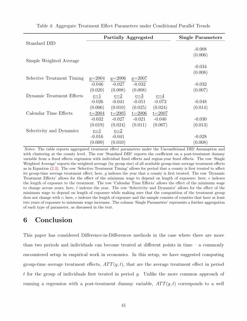
Table 4: Aggregate Treatment Effect Parameters under Conditional Parallel Trends

Partially Aggregated Single ParametersStandard DID

-0.008(0.006)

Simple Weighted Average-0.034(0.008)

Selective Treatment Timing g=2004 g=2006 g=2007-0.046 -0.027 -0.032 -0.032(0.020) (0.008) (0.008) (0.007)

Dynamic Treatment Effects e=1 e=2 e=3 e=4-0.026 -0.041 -0.051 -0.073 -0.048(0.006) (0.010) (0.025) (0.024) (0.014)

Calendar Time Effects t=2004 t=2005 t=2006 t=2007-0.032 -0.027 -0.021 -0.040 -0.030(0.019) (0.024) (0.011) (0.007) (0.013)

Selectivity and Dynamics e=1 e=2-0.016 -0.041 -0.028(0.009) (0.010) (0.008)

Notes: The table reports aggregated treatment effect parameters under the Unconditional DID Assumption andwith clustering at the county level. The row ‘Standard DID’ reports the coefficient on a post-treatment dummyvariable from a fixed effects regression with individual fixed effects and region-year fixed effects. The row ‘SingleWeighted Average’ reports the weighted average (by group size) of all available group-time average treatment effectsas in Equation (2.3). The row ‘Selective Treatment Timing’ allows for period that a county is first treated to affectits group-time average treatment effect; here, g indexes the year that a county is first treated. The row ‘DynamicTreatment Effects’ allows for the effect of the minimum wage to depend on length of exposure; here, e indexesthe length of exposure to the treatment. The row ‘Calendar Time Effects’ allows the effect of the minimum wageto change across years; here, t indexes the year. The row ‘Selectivity and Dynamics’ allows for the effect of theminimum wage to depend on length of exposure while making sure that the composition of the treatment groupdoes not change with e; here, e indexes the length of exposure and the sample consists of counties that have at leasttwo years of exposure to minimum wage increases. The column ‘Single Parameters’ represents a further aggregationof each type of parameter, as discussed in the text.

6 Conclusion

This paper has considered Difference-in-Differences methods in the case where there are more

than two periods and individuals can become treated at different points in time – a commonly

encountered setup in empirical work in economics. In this setup, we have suggested computing

group-time average treatment effects, ATT (g, t), that are the average treatment effect in period

t for the group of individuals first treated in period g. Unlike the more common approach of

running a regression with a post-treatment dummy variable, ATT (g, t) corresponds to a well

41

defined treatment effect parameter. And once ATT (g, t) has been obtained for different values of

g and t, they can be aggregated into a single parameter, though the exact implementation depends

on the particular case. We view such a flexibility as a plus of our proposed methodology.

Given that our nonparametric identification results are constructive, we proposed to estimate

ATT (g, t) using its sample analogue. We established consistency and asymptotically normality

of the proposed estimators, and proved the validity of a powerful, but easy to implement, multi-

plier bootstrap procedure to construct simultaneous confidence bands for ATT (g, t). Importantly,

we have also proposed a new pre-test for the the reliability of the conditional parallel trends

assumption.

We applied our approach to study the effect of minimum wage increases on teen employment.

We found some evidence that increasing the minimum wage led to reductions in teen employment

and found strikingly different results from the more common approach of interpreting the coef-

ficient on a post-treatment dummy variable as the effect of the minimum wage on employment.

However, using the pre-tests developed in the current paper, we found evidence against both the

unconditional and conditional parallel trends assumption.

42

(For Online Publication) Appendix A: Mathematical Proofs

We provide the proofs of our results in this appendix. Before proceeding, we first state and prove

several auxiliary lemmas that help us proving our main theorems.

Let

ATTX(g, t) = E[Yt(1)− Yt(0)|X,Gg = 1].

Lemma A.1. Under Assumptions 1-4, and for 2 ≤ g ≤ t ≤ T ,

ATTX(g, t) = E[Yt − Yg−1|X,Gg = 1]− E[Yt − Yg−1|X,C = 1] a.s..

Proof of Lemma A.1: In what follows, take all equalities to hold almost surely (a.s.). Notice

that for identifying ATTX(g, t), the key term is E[Yt(0)|X,Gg = 1]. And notice that for h > s,

E[Ys(0)|X,Gs = 1] = E[Ys|X,Gh = 1], which holds because in time periods before an individual

is first treated, their untreated potential outcomes are observed outcomes. Also, note that, for

2 ≤ g ≤ t ≤ T ,

E[Yt(0)|X,Gg = 1] = E[∆Yt(0)|X,Gg = 1] + E[Yt−1(0)|X,Gg = 1] (A.1)

= E[∆Yt|X,C = 1] + E[Yt−1(0)|X,Gg = 1],

where the first equality holds by adding and subtracting E[Yt−1(0)|X,Gg = 1] and the second

equality holds by Assumption 2. If g = t− 1, then the last term in the final equation is identified;

otherwise, one can continue recursively in similar way to (A.1) but starting with E[Yt−1(0)|X,Gg =

1]. As a result,

E[Yt(0)|X,Gg = 1] =

t−g∑j=0

E[∆Yt−j|X,C = 1] + E[Yg−1|X,Gg = 1]

= E[Yt − Yg−1|X,C = 1] + E[Yg−1|X,Gg = 1]. (A.2)

Combining (A.2) with the fact that, for all g ≤ t, E[Yt(1)|X,Gg = 1] = E[Yt|X,Gg = 1] (which

holds because observed outcomes for group g in period t with g ≤ t are treated potential outcomes),

implies the result. �

43

Next, recall that

πg = arg maxπ

∑i:Gig+Ci=1

Gig ln (pg (X ′iπ)) + (1−Gig) ln (1− pg (X ′iπ)) ,

pg = ∂pg (u)/ ∂u, pg (X) = pg(X ′π0

g

), and π0

g is the true, unknown vector of parameter indexed

the generalized propensity score pg (X) = E [Gg = 1|X,Gg + C = 1].

Lemma A.2. Under Assumption 5,

√n(πg − π0

g

)=

1√n

n∑i=1

ξπg (Wi) + op (1) ,

where

ξπg (W) = E

[(Gg + C) pg (X)2

pg (X) (1− pg (X))XX ′

]−1X

(Gg + C) (Gg − pg (X)) pg (X)

pg (X) (1− pg (X)).

Proof of Lemma A.2: Let ngc =∑n

i=1 (Ci +Gig). Under Assumption 5, from Theorem 5.39

and Example 5.40 in van der Vaart (1998), we have

√ngc(πg − π0

g

)=

1√ngc

∑i:Gig+Ci=1

E

[pg (X)2

pg (X) (1− pg (X))XX ′

∣∣∣Gg + C = 1

]−1Xi

(Gig − pg (Xi)) pg (Xi)

pg (Xi) (1− pg (Xi))

+op (1)

=E [Gg + C]√ngc

n∑i=1

E

[(Gg + C) pg (X)2

pg (X) (1− pg (X))XX ′

]−1Xi

(Gig + Ci) (Gig − pg (Xi)) pg (Xi)

pg (Xi) (1− pg (Xi))

+op (1)

=En [Gg + C]√ngc

n∑i=1

ξπg (Wi) +op (1)

=

√ngc

n

n∑i=1

ξπg (Wi) +op (1) .

Thus,

√n(πg − π0

g

)=

√n

√ngc

√ngc(πg − π0

g

)=

1√n

n∑i=1

ξπg (Wi) + op (1) ,

44

and the proof is complete. �

For an arbitrary π, let pg (x; π) = pg (x′π) , pg (x; π) = pg (x′π), for all g = 2, . . . , T . Define

the classes of functions,

H1,g =

{(x, c) 7→ c

pg (x; π)

1− pg (x; π): π ∈ Πg

},

H2,g =

{(x, c, yt, yg−1) 7→ c

pg (x; π) (yt − yg−1)1− pg (x; π)

: π ∈ Πg

}H3,g =

{(x, c, yt, yg−1) 7→ x

c pg (x; π) (yt − yg−1)(1− pg (x; π))2

: π ∈ Πg

},

H4,g =

{(x, c) 7→ x

c pg (x; π)

(1− pg (x; π))2: π ∈ Πg

},

H5,g =

{(x, c, gg) 7→ x

(gg + c) (gg − pg (x; π)) pg (x; π)

pg (x; π) (1− pg (x; π)): π ∈ Πg

}.

Lemma A.3. Under Assumptions 1 and 5, for all g = 2, . . . , T , t = 2, . . . , T , the classes of

functions Hj,g, j = {1, 2 . . . , 5}, are Donsker.

Proof of Lemma A.3: This follows from Example 19.7 in van der Vaart (1998).

Lemma A.4. Under Assumptions 1 and 5, the null hypothesis

H0 : E[Yt − Yt−1|X,Gg = 1]− E[Yt − Yt−1|X,C = 1] = 0 a.s.for all 2 ≤ t < g ≤ T ,

can be equivalently written as

H0 : E

Gg

E [Gg]−

pg (X)C

1− pg (X)

E[pg (X)C

1− pg (X)

] (Yt − Yt−1)

∣∣∣∣∣∣∣∣X = 0 a.s.for all 2 ≤ t < g ≤ T .

Proof of Lemma A.4: First note that

E[Yt − Yt−1|X,Gg = 1] = E[Gg (Yt − Yt−1) |X,Gg = 1]

= E[

Gg

E [Gg|X](Yt − Yt−1)

∣∣∣∣X] .45

Analogously,

E[Yt − Yt−1|X,C = 1] = E[

C

E [C|X](Yt − Yt−1)

∣∣∣∣X] ,implying that

E[Yt − Yt−1|X,Gg = 1]− E[Yt − Yt−1|X,C = 1] = 0 a.s.for all 2 ≤ t < g ≤ T .

⇐⇒

E[(

Gg

E [Gg|X]− C

E [C|X]

)(Yt − Yt−1)

∣∣∣∣X] = 0 a.s.for all 2 ≤ t < g ≤ T .

Given that under Assumptions 4 and 5, E [Gg + C|X] > 0 a.s., we have that

E[(

Gg

E [Gg|X]− C

E [C|X]

)(Yt − Yt−1)

∣∣∣∣X] = 0 a.s.for all 2 ≤ t < g ≤ T

if an only if

E[E [Gg + C|X]

(Gg

E [Gg|X]− C

E [C|X]

)(Yt − Yt−1)

∣∣∣∣X] = 0 a.s.for all 2 ≤ t < g ≤ T . (A.3)

By noticing that

pg (X) =E [Gg|X]

E [Gg + C|X], 1− pg (X) =

E [C|X]

E [Gg + C|X],

and that both of these are bounded away from zero under Assumption 5, we can rewrite (A.3) as

E

Gg

E [Gg]−

pg (X)C

1− pg (X)

E[pg (X)C

1− pg (X)

] (Yt − Yt−1)

∣∣∣∣∣∣∣∣X = 0 a.s.for all 2 ≤ t < g ≤ T ,

since

E[

pg (X)C

(1− pg(X))

]= E

[E [Gg|X,C +Gg = 1]C

E [C|X,C +Gg = 1]

]= E

[E [Gg|X]C

E [C|X]

]= E

[E [Gg|X]E [C|X]

E [C|X]

]= E [E [Gg|X]]

= E [Gg] . (A.4)

46

This completes the proof.�

Now, we are ready to proceed with the proofs of our main theorems.

Proof of Theorem 1: Given the result in Lemma A.1,

ATT (g, t) = E[ATTX(g, t)|Gg = 1]

= E[E[Yt − Yg−1|X,Gg = 1]− E[Yt − Yg−1|X,C = 1]

∣∣∣Gg = 1]

:= E[AX |Gg = 1]− E[BX |Gg = 1],

and we consider each term separately. For the first term

E[AX |Gg = 1] = E[Yt − Yg−1|Gg = 1]

= E[

Gg

E [Gg](Yt − Yg−1)

]. (A.5)

For the second term, by repetition of the law of iterated expectations, we have

E[BX |Gg = 1] = E[E[Yt − Yg−1|X,C = 1]

∣∣∣Gg = 1]

= E[GgE[C(Yt − Yg−1)|X,C = 1]

∣∣∣Gg = 1]

= E[GgE

[C

(1− pg(X))(Yt − Yg−1)

∣∣X,Gg + C = 1

] ∣∣∣Gg = 1

]

=

E[GgE

[C

(1− pg(X))(Yt − Yg−1)

∣∣X,Gg + C = 1

] ∣∣∣Gg + C = 1

]E [Gg|Gg + C = 1]

=

E[E[

pg (X)C

(1− pg(X))(Yt − Yg−1)

∣∣X,Gg + C = 1

] ∣∣∣Gg + C = 1

]E [Gg|Gg + C = 1]

= E [Gg]−1 E

[E [Gg + C|X]E

[pg (X)C

(1− pg(X))(Yt − Yg−1)

∣∣X,Gg + C = 1

]]= E [Gg]

−1 E[E[

pg (X)C

(1− pg(X))(Yt − Yg−1)

∣∣X]]= E [Gg]

−1 E[E[

pg (X)C

(1− pg(X))(Yt − Yg−1)

]]

=

E[

pg (X)C

(1− pg(X))(Yt − Yg−1)

]E[

pg (X)C

(1− pg(X))

] , (A.6)

47

where (A.6) follows from (A.4). The proof is completed by combining (A.5) and (A.6). �

Proof of Theorem 2: Remember that

ATT (g, t) = En[

Gg

En [Gg](Yt − Yg−1)

]− En

pg (X)C

1− pg (X)

En[pg (X)C

1− pg (X)

] (Yt − Yg−1)

,:= ATT g(g, t)− ATTC(g, t),

and

ATT (g, t) = E[

Gg

E [Gg](Yt − Yg−1)

]− E

pg (X)C

1− pg (X)

E[pg (X)C

1− pg (X)

] (Yt − Yg−1)

:= ATTg(g, t)− ATTC(g, t).

In what follows we will separately show that, for 2 ≤ g ≤ t ≤ T ,

√n(ATT g(g, t)− ATTg(g, t)

)=

1√n

n∑i=1

ψGgt(Wi) + op (1) , (A.7)

and√n(ATTC(g, t)− ATTC(g, t)

)=

1√n

n∑i=1

ψCgt(Wi) + op (1) . (A.8)

Then,√n(ATT (g, t)− ATT (g, t)) =

1√n

n∑i=1

ψgt(Wi) + op(1)

hold from (A.7) and (A.8), and the asymptotic normality result follows from the application of

the central limit theorem.

Let βg = E [Gg] and βg = En [Gg], and note that

√n(βg − βg

)=

1√n

n∑i=1

(Gig − E [Gg]) .

Then, for all 2 ≤ g ≤ t ≤ T , by the continuous mapping theorem,

√n(ATT g(g, t)− ATTg(g, t)

)=

1

βg

√n (En [Gg (Yt − Yg−1)]− E [Gg (Yt − Yg−1)])

48

− E [Gg (Yt − Yg−1)]√n

(1

βg− 1

βg

)

=1

βg

1√n

n∑i=1

(Gig (Yit − Yig−1)− E [Gg (Yt − Yg−1)])

− E [Gg (Yt − Yg−1)]β2g

√n(βg − βg

)+ op (1)

=1√n

n∑i=1

(Gig (Yit − Yig−1)

βg− GigE [Gg (Yt − Yg−1)]

β2g

)+ op (1)

=1√n

n∑i=1

Gig ((Yit − Yig−1)− ATTg(g, t))βg

+ op (1)

:=1√n

n∑i=1

ψGgt(Wi) + op (1) ,

concluding the proof of (A.7).

Next we focus on (A.8). For an arbitrary function g, let

w (g) =g (X)C

1− g (X),

and note that

√n(ATTC(g, t)− ATTC(g, t)

)=

1

En [w (pg)]

√n (En [w (pg) (Yt − Yg−1)]− E [w (pg) (Yt − Yg−1)])

− E [w (pg) (Yt − Yg−1)]En [w (pg)]E [w (pg)]

√n (En [w (pg)]− E [w (pg)])

:=1

En [w (pg)]·√nAn (pg)−

ATTC(g, t)

En [w (pg)]·√nBn (pg) .

From Assumption 5, Lemmas A.2 and A.3, and the continuous mapping theorem,

1

En [w (pg)]=

1

E [w (pg)]+ op (1) ,

ATTC(g, t)

En [w (pg)]=ATTC(g, t)

E [w (pg)]+ op (1) .

Thus,

√n(ATTC(g, t)− ATTC(g, t)

)=

1

E [w (pg)]·√nAn (pg)

− ATTC(g, t)

E [w (pg)]·√nBn (pg) + op (1) (A.9)

49

Applying a classical mean value theorem argument,

An (pg) = En [w (pg) (Yt − Yg−1)]− E [w (pg) (Yt − Yg−1)]

+ En

[X

(C

1− pg (X; πg)

)2

pg (X; πg) (Yit − Yig−1)

]′ (πg − π0

g

),

where π is an intermediate point that satisfies∣∣πg − π0

g

∣∣ ≤ ∣∣πg − π0g

∣∣ a.s. Thus, by Assumption 5,

Lemmas A.2 and A.3, and the Classical Glivenko-Cantelli’s theorem,

An (pg) = En [w (pg) (Yt − Yg−1)− E [w (pg) (Yt − Yg−1)]] (A.10)

+ E

[X

(C

1− pg (X)

)2

pg (X) (Yit − Yig−1)

]′ (πg − π0

g

)+ op

(n−1/2

). (A.11)

Analogously,

Bn (pg) = En [w (pg)− E [w (pg)]]

+ E

[X

(C

1− pg (X)

)2

pg (X)

]′ (πg − π0

g

)+ op

(n−1/2

). (A.12)

Then, (A.9), (A.10), (A.12) and Lemma A.2 yield (A.8), concluding the proof.�

Proof of Theorem 3: Note that, by the conditional multiplier central limit theorem, see Lemma

2.9.5 in van der Vaart and Wellner (1996), as n→∞,

1√n

n∑i=1

Vi ·Ψg≤t(Wi)d→ N(0,Σ), (A.13)

where Σ = E[Ψg≤t(W)Ψg≤t(W)′]. Thus, to conclude the proof that

√n(ATT

∗g≤t − ATT g≤t

)d→∗N(0,Σ),

it suffices to show that, for all 2 ≤ g ≤ t ≤ T ,

1√n

n∑i=1

Vi ·[ψgt(Wi)− ψgt(Wi)

]= op∗ (1) .

50

Towards this, note that

1√n

n∑i=1

Vi ·[ψgt(Wi)− ψgt(Wi)

]=

1√n

n∑i=1

Vi ·[ψGgt(Wi)− ψGgt(Wi)

](A.14)

− 1√n

n∑i=1

Vi ·[ψCgt(Wi)− ψCgt(Wi)

],

where

ψGgt(W) =Gg

En [Gg]

[(Yt − Yg−1)− ATT g(g, t)

],

and

ψCgt(W) =w (pg)

En [w (pg)]

[(Yit − Yig−1)− ATTC(g, t)

]+ M ′

gt ξπg (W) ,

with

w (pg) =pg (X)C

1− pg (X),

Mgt =

En

[X

(C

1− pg (X)

)2 pg (X)[(Yit − Yig−1)− ATT g(g, t)

]]En [w (pg)]

,

ξπg (W) = En

[(Gg + C) pg (X)2

pg (X) (1− pg (X))XX ′

]−1X

(Gg + C) (Gg − pg (X)) pg (X)

pg (X) (1− pg (X)).

We will show that each term in (A.14) is op∗ (1). For the first term in (A.14), we have

1√n

n∑i=1

Vi ·[ψGgt(Wi)− ψGgt(Wi)

]=

[1

En [Gg]− 1

E [Gg]

]1√n

n∑i=1

Vi ·Gig (Yit − Yig−1)

−[ATT g(g, t)− ATTg(g, t)

] 1√n

n∑i=1

Vi ·Gig,

= op∗ (1) , (A.15)

where the last equality follows from the results in Theorem 1, together with the law of large

numbers, continuous mapping theorem, and Lemma 2.9.5 in van der Vaart and Wellner (1996).

51

For the second term in (A.14), we have

1√n

n∑i=1

Vi ·[ψCgt(Wi)− ψCgt(Wi)

]=

1

En [w (pg)]

1√n

n∑i=1

Vi · (wi (pg)− wi (pg)) (Yit − Yig−1)

+

(1

En [w (pg)]− 1

E [w (pg)]

)1√n

n∑i=1

Vi · wi (pg) (Yit − Yig−1)

+(Mgt −Mgt

) 1√n

n∑i=1

Vi · ξπg (Wi) .

+ Mgt1√n

n∑i=1

Vi ·(ξπg (Wi)− ξπg (Wi)

):= A1n + A2n + A3n + A4n.

From Lemma A.3, we have that H1,g, H2,g, H3,g and H5,g are Donsker, and by Assumption 5,

E [w (pg)] it is bounded away from zero. Thus, by a stochastic equicontinuity argument, Glivenko-

Cantelli’s theorem, continuous mapping theorem, and Theorem 2.9.6 in van der Vaart and Wellner

(1996),

A1n = op∗ (1) , A2n = op∗ (1) , A3n = op∗ (1) , and A4n = op∗ (1) ,

implying that

1√n

n∑i=1

Vi ·[ψCgt(Wi)− ψCgt(Wi)

]= op∗ (1) . (A.16)

From (A.13)-(A.16), it follows that

√n(ATT

∗g≤t − ATT g≤t

)d→∗N(0,Σ).

Finally, by the continuous mapping theorem, see e.g. Theorem 10.8 in Kosorok (2008), for any

continuous functional Γ(·)

Γ(√

n(ATT

∗g≤t − ATT g≤t

))d→∗

Γ (N(0, V )) ,

concluding our proof. �

Proof of Theorem 4: In order to prove the first part of Theorem 4, we first show that, under

52

H0, for all 2 ≤ t < g ≤ T ,

J(u, g, t, pg) = En[ψtestugt (Wi)

]+ op

(n−1/2

),

Towards this end, we write

J(u, g, t, pg) = En[

Gg

En [Gg]1(X ≤ u) (Yt − Yt−1)

]

− En

pg (X)C

1− pg (X)

En[pg (X)C

1− pg (X)

]1(X ≤ u) (Yt − Yt−1)

:= JG(u, g, t, pg)− JC(u, g, t, pg),

and analyze each term separately.

As in the proof of Theorem 1, let βg = E [Gg] and βg = En [Gg]. Applying a classical mean

value theorem argument, uniformly in u ∈ X ,

JG(u, g, t, pg) = En[Gg

βg1(X ≤ u) (Yt − Yt−1)

]− En [Gg1(X ≤ u) (Yt − Yt−1)]

β2g

· En [Gg − E [Gg]] .

where βg is an intermediate point that satisfies∣∣βg − βg∣∣ ≤ ∣∣∣βg − βg∣∣∣ a.s.. Define the class of

functions

H6,g = {(x, gg, yt, yt−1) 7→ gg (yt − yt−1) 1 {x ≤ u} : u ∈ X} .

By Example 19.11 in van der Vaart (1998), H6,g is Donsker under Assumption 5. Furthermore,

En [Gg − E [Gg]] = Op

(n−1/2

).

Thus, by the Glivenko-Cantelli’s theorem and the continuous mapping theorem, uniformly in

u ∈ X ,

JG(u, g, t, pg) = En[

Gg

E [Gg]1(X ≤ u) (Yt − Yt−1)

]− JG(u, g, t, pg)

E [Gg]· En [Gg − E [Gg]] + op

(n−1/2

)

53

= En[wGg((Yt − Yt−1) 1(X ≤ u)− E

[wGg 1(X ≤ u) (Yt − Yt−1)

])]+ JG(u, g, t, pg)

(A.17)

+ op(n−1/2

),

where

JG(u, g, t, pg) = E[

Gg

E [Gg]1(X ≤ u) (Yt − Yt−1)

].

We analyze JC(u, g, t, pg) next. Applying a classical mean value theorem argument, uniformly

in u ∈ X ,

JC(u, g, t, pg) = JC(u, g, t, pg)

+

En

[X

C pg (X; πg)

(1− pg (X; πg))21(X ≤ u) (Yt − Yt−1)

]

En[pg (X; πg)C

1− pg (X; πg)

]′

(πg − π0

g

)

−En

[X

C pg (X; πg)

(1− pg (X; πg))2

]′En[pg (X; πg)C

1− pg (X; πg)

] En[pg (X; πg)C

1− pg (X; πg)1(X ≤ u) (Yt − Yt−1)

]En[pg (X; πg)C

1− pg (X; πg)

] (πg − π0

g

)

where π is an intermediate point that satisfies∣∣πg − π0

g

∣∣ ≤ ∣∣πg − π0g

∣∣ a.s, and

JC(u, g, t, pg) =

En[pg (X)C

1− pg (X)1(X ≤ u) (Yt − Yt−1)

]En[pg (X)C

1− pg (X)

] .

Define the classes of functions

H7,g =

{(x, c, yt, yt−1) 7→

pg (x; π)

1− pg (x; π)c (yt − yt−1) 1 {x ≤ u} : π ∈ Πg, u ∈ X

},

H8,g =

{(x, c, yt, yt−1) 7→ x

pg (x; π) c (yt − yt−1) 1 {x ≤ u}(1− pg (x; π))2

: π ∈ Πg, u ∈ X

},

H9,g =

{(x, c) 7→ cpg (x; π)

1− pg (x; π): π ∈ Πg,

},

H10,g =

{(x, c) 7→ x

pg (x; π) c

(1− pg (x; π))2: π ∈ Πg

}.

54

By Examples 19.7, 19.11, and 19.20 in van der Vaart (1998), all these classes of functions are

Donsker under Assumption 5. Thus, by the Glivenko-Cantelli’s theorem, continuous mapping

theorem, and Lemma A.2, uniformly in u ∈ X ,

JC(u, g, t, pg) = JC(u, g, t, pg) +M test ′ugt

(πg − π0

g

)+ op

(n−1/2

), (A.18)

for every g, t.

Denote

βCg = En[pg (X)C

1− pg (X)

], βCg = E

[pg (X)C

1− pg (X)

].

Applying a classical mean value theorem argument, we have

JC(u, g, t, pg) =

En[pg (X)C

1− pg (X)1(X ≤ u) (Yt − Yt−1)

]E[pg (X)C

1− pg (X)

]

−En[pg (X)C

1− pg (X)1(X ≤ u) (Yt − Yt−1)

](βCg)2 · En

[pg (X)C

1− pg (X)− E

[pg (X)C

1− pg (X)

]]

where βCg is an intermediate point that satisfies∣∣βCg − βCg ∣∣ ≤ ∣∣∣βCg − βCg ∣∣∣ a.s.. Since H7,g is a

Donsker Class of functions and

En[pg (X)C

1− pg (X)− E

[pg (X)C

1− pg (X)

]]= Op

(n−1/2

),

we have that, by the Glivenko-Cantelli’s theorem and the continuous mapping theorem, uniformly

in u ∈ X ,

JC(u, g, t, pg) = En[wCg (Yt − Yt−1) 1(X ≤ u)

]−

E[wCg (Yt − Yt−1) 1(X ≤ u)

]E[pg (X)C

1− pg (X)

] · En[pg (X)C

1− pg (X)− E

[pg (X)C

1− pg (X)

]]+ op

(n−1/2

)

= En[wCg

((Yt − Yt−1) 1(X ≤ u)− E

[wCg 1(X ≤ u) (Yt − Yt−1)

])]+ JC(u, g, t, pg)

(A.19)

+ op(n−1/2

).

55

Hence, from (A.17), (A.18), (A.19), and the asymptotic linear representation of(πg − π0

g

)in

Lemma A.2, for every g, t,

J(u, g, t, pg) = En[ψtestugt (W)

]+ (JG(u, g, t, pg)− JC(u, g, t, pg)) + op

(n−1/2

)(A.20)

By noticing that under H0, JG(u, g, t, pg) = JC(u, g, t, pg) for all u ∈ X , (g, t) such that

2 ≤ t < g ≤ T , we have that, under H0, uniformly in u ∈ X , for all 2 ≤ t < g ≤ T

J(u, g, t, pg) = En[ψtestugt (Wi)

]+ op

(n−1/2

).

In order to show that√nJg>t (u) ⇒ G(u) in l∞ (X ), it suffices to show that the class of

functions

H10 ={

(x, gg, c, yt, yt−1) 7→ ψtestugt : u ∈ X , 2 ≤ t < g ≤ T}

is Donsker. This follows straightforwardly from the the previously discussed Donsker results and

Example 19.20 in van der Vaart (1998). Finally,

CvMnd→∫X|G(u)|2M FX (du)

follows from the continuous mapping theorem,

supu∈X|Fn,X (u)− FX (u)| = oa.s. (1) ,

and the Helly-Bray Theorem.

Next, we study the behavior of CvMn under H1. First, note that under H1, for some u ∈ X ,

and some (g, t), 2 ≤ t < g ≤ T ,

J(u, g, t, pg) 6= 0 .

Thus, from (A.20), under H1, uniformly in u ∈ X ,

√nJg>t (u) = Op

(n1/2

),

implying that CvMn diverges to infinity under H1. Because cCvMα = O (1) a.s., as n→∞,

P(CvMn > cCvMα

)→ 1,

56

concluding the proof of Theorem 4. �

Proof of Theorem 5: In the proof of Theorem 4, we have shown that

H11 ={

(x, gg, c, yt, yt−1) 7→ ψtestugt : u ∈ X , 2 ≤ t < g ≤ T}

is a Donsker class of functions. Then, by the conditional multiplier functional central limit theorem,

see Theorem 2.9.6, in van der Vaart and Wellner (1996), as n→∞,

1√n

n∑i=1

Vi ·Ψtestg>t(Wi)⇒∗ G(u) in l∞ (X ) ,

where G(u) in l∞ (X ) is the same Gaussian process of Theorem 4 and ⇒∗

indicates weak conver-

gence in probability under the bootstrap law. Thus, to conclude the proof it suffices to show that,

for all 2 ≤ t < g ≤ T , uniformly in u ∈ X ,

1√n

n∑i=1

Vi ·[ψtestugt (Wi)− ψtestugt (Wi)

]= op∗ (1) . (A.21)

The proof of (A.21) follows exactly the same steps as the proof of Theorem (3), and is therefore

omitted.�

References

Abadie, A. (2005), “Semiparametric difference-in-difference estimators,” Review of Economic Stud-

ies, 72, 1–19.

Amemiya, T. (1985), Advanced Econometrics, Cambridge: Harvard University Press.

Angrist, J. D., and Pischke, J.-S. (2008), Mostly Harmless Econometrics: An Empiricist’s Com-

panion, : Princeton University Press.

Athey, S., and Imbens, G. W. (2006), “Identification and inference in nonlinear difference in

differences models,” Econometrica, 74(2), 431–497.

Autor, D. H., Kerr, W. R., and Kugler, A. D. (2007), “Does Employment Protection Reduce

Productivity? Evidence From US States,” The Economic Journal, 117(521), F189–F217.

Belloni, A., Chernozhukov, V., Fernandez-Val, I., and Hansen, C. (2017), “Program Evaluation

and Causal Inference With High-Dimensional Data,” Econometrica, 85(1), 233–298.

Belman, D., and Wolfso, P. J. (2014), What does the minimum wage do?, Kalamazoo, MI: W.E.

Upjohn Institute for Employment Research.

57

Bertrand, M., Duflo, E., and Mullainathan, S. (2004), “How Much Should We Trust Differences-

In-Differences Estimates?,” The Quarterly Journal of Economics, 119(1), 249–275.

Bierens, H. J. (1982), “Consistent model specification tests,” Journal of Econometrics,

20(1982), 105–134.

Bierens, H. J., and Ploberger, W. (1997), “Asymptotic theory of integrated conditional moment

tests,” Econometrica, 65(5), 1129–1151.

Blundell, R., Dias, M. C., Meghir, C., and van Reenen, J. (2004), “Evaluating the Employment

Impact of a Mandatory Job Search Program,” Journal of the European Economic Association,

2(4), 569–606.

Bonhomme, S., and Sauder, U. (2011), “Recovering distributions in difference-in-differences mod-

els: a comparison of selective and comprehensive schooling,” , 93(May), 479–494.

Borusyak, K., and Jaravel, X. (2017), “Revisiting Event Study Designs,” Mimeo, pp. 1–33.

Botosaru, I., and Gutierrez, F. H. (2017), “Difference-in-differences when the treatment status is

observed in only one period,” Journal of Applied Econometrics, (March 2017), 73–90.

Busso, M., Dinardo, J., and McCrary, J. (2014), “New Evidence on the Finite Sample Properties

of Propensity Score Reweighting and Matching Estimators,” The Review of Economics and

Statistics, 96(5), 885–895.

Callaway, B., Li, T., and Oka, T. (2018), “Quantile Treatment Effects in Difference in Differ-

ences Models Under Dependence Restrictions and with Only Two Time Periods,” Journal of

Econometrics, Forthcoming.

Card, D., and Krueger, A. B. (1994), “Minimum Wages and Employment: A Case Study of the

Fast-Food Industry in New Jersey and Pennsylvania,” American Economic Review, 84(4), 772–

793.

Cheng, G., Yu, Z., and Huang, J. Z. (2013), “The cluster bootstrap consistency in generalized

estimating equations,” Journal of Multivariate Analysis, 115, 33–47.

Chernozhukov, V., Fernandez-Val, I., Hahn, J., and Newey, W. (2013), “Average and Quantile

Effects in Nonseparable Panel Models,” Econometrica, 81(2), 535–580.

Chernozhukov, V., Fernandez-Val, I., and Luo, Y. (2017), “The sorted effects method: discovering

heterogeneous effects beyond their averages,” Arxiv preprint arXiv:1512.05635, .

de Chaisemartin, C., and D’Haultfoeuille, X. (2016), “Double fixed effects estimators with hetero-

geneous treatment effects,” Working Paper, (Did), 1–23.

de Chaisemartin, C., and D’Haultfœuille, X. (2017), “Fuzzy Differences-in-Differences,” The Re-

view of Economic Studies, (February), 1–30.

Donald, S. G., and Hsu, Y.-C. (2014), “Estimation and inference for distribution functions and

quantile functions in treatment effect models,” Journal of Econometrics, 178(3), 383–397.

Doucouliagos, H., and Stanley, T. D. (2009), “Publication selection bias in minimum-wage re-

search? A meta-regression analysis,” British Journal of Industrial Relations, 47(2), 406–428.

58

Dube, A., Lester, T. W., and Reich, M. (2010), “Minimum Wage Effects Across State Borders:

Estimates Using Contiguous Counties,” Review of Economics and Statistics, 92(4), 945–964.

Dube, A., Lester, T. W., and Reich, M. (2016), “Minimum wage shocks, employment flows, and

labor market frictions,” Journal of Labor Economics, 34(3), 663–704.

Escanciano, J. C. (2006a), “A consistent diagnostic test for regression models using projections,”

Econometric Theory, 22, 1030–1051.

Escanciano, J. C. (2006b), “Goodness-of-Fit Tests for Linear and Nonlinear Time Series Models,”

Journal of the American Statistical Association, 101(474), 531–541.

Escanciano, J. C. (2008), “Joint and marginal specification tests for conditional mean and variance

models,” Journal of Econometrics, 143(1), 74–87.

Freyberger, J., and Rai, Y. (2018), “Uniform confidence bands: characterization and optimality,”

Journal of Econometrics, Forthcoming.

Gine, E., and Zinn, J. (1990), “Bootstrapping general empirical measures,” The Annals of Proba-

bility, 18(2), 851–869.

Gonzalez-Manteiga, W., and Crujeiras, R. M. (2013), “An updated review of Goodness-of-Fit tests

for regression models,” Test, 22(3), 361–411.

Goodman-Bacon, A. (2017), “Difference-in-Differences with Variation in Treatment Timing,”

Working Paper, .

Heckman, J. J., Ichimura, H., Smith, J., and Todd, P. (1998), “Characterizing selection bias using

experimental data,” Econometrica, 66(5), 1017–1098.

Heckman, J. J., Ichimura, H., and Todd, P. (1997), “Matching as an econometric evaluation

estimator: Evidence from evaluating a job training programme,” The Review of Economic

Studies, 64(4605-654).

Horvitz, D. G., and Thompson, D. J. (1952), “A Generalization of Sampling Without Replacement

From a Finite Universe,” Journal of the American Statistical Association, 47(260), 663–685.

Jacobson, L. S., Lalonde, R. J., and Sullivan, D. G. (1993), “Earnings Losses of Displaced Work-

ers,” American Economic Review, 83(4), 685–709.

Jardim, E., Long, M., Plotnick, R., van Inwegen, E., Vigdor, J., and Wething, H. (2017), Minimum

Wage Increases, Wages, and Low-Wage Employment: Evidence from Seattle,, Technical report,

National Bureau of Economic Research, Cambridge, MA.

Kline, P., and Santos, A. (2012), “A Score Based Approach to Wild Bootstrap Inference,” Journal

of Econometric Methods, 1(1), 1–40.

Kosorok, M. R. (2008), Introduction to empirical processes and semiparametric inference, New

York, NY: Springer.

MacKinnon, J. G., and Webb, M. D. (2016), “Difference-in-Differences Inference with Few Treated

Clusters,” Queen’s Economics Department Working Papers No. 1355, pp. 1–44.

59

MacKinnon, J. G., and Webb, M. D. (2017), “The wild bootstrap for few (treated) clusters,” The

Econometrics Journal, 20, 1–22.

Mammen, E. (1993), “Bootstrap and wild bootstrap for high dimensional linear models,” The

Annals of Statistics, 21(1), 255–285.

Meer, J., and West, J. (2016), “Effects of the Minimum Wage on Employment Dynamics,” Journal

of Human Resources, 51(2), 500–522.

Montiel Olea, J. L., and Plagborg-Møller, M. (2017), “Simultaneous Confidence Bands: Theory,

Implementation, and an Application to SVARs,” Working Paper, pp. 1–64.

Neumark, D., Salas, J. M., and Wascher, W. (2014), “Revisiting the minimum wage-employment

debate: Throwing out the baby with the bathwater?,” Industrial and Labor Relations Review,

67(SUPPL), 608–648.

Neumark, D., and Wascher, W. (1992), “Evidence on Employment Effects of Minimum Wages

and Subminimum Wage Provisions from Panel Data on State Minimum Wage Laws,” Industrial

and Labor Relations Review, 46(1), 55–81.

Neumark, D., and Wascher, W. (2000), “Minimum Wages and Employment: A Case Study of the

Fast-Food Industry in New Jersey and Pennsylvania: Comment,” American Economic Review,

90(5), 1362–1396.

Neumark, D., and Wascher, W. L. (2008), Minimum Wages, Cambridge, MA: The MIT Press.

Oreopoulos, P., von Wachter, T., and Heisz, A. (2012), “The Short- and Long-Term Career Effects

of Graduating in a Recession,” American Economic Journal: Applied Economics, 4(1), 1–29.

Qin, J., and Zhang, B. (2008), “Empirical-Likelihood-Based Difference-in-Differences Estimators,”

Journal of the Royal Statistical Society. Series B (Methodological), 75(8), 329–349.

Sant’Anna, P. H. C. (2016), “Program Evaluation with Right-Censored Data,” ArXiv preprint

arXiv:1604.02642, .

Sant’Anna, P. H. C. (2017), “Nonparametric Tests for Treatment Effect Heterogeneity with Du-

ration Outcomes,” Arxiv preprint arXiv:1612.02090, .

Sant’Anna, P. H. C., and Song, X. (2018), “Specification Tests for the Propensity Score,” Arxiv

preprint arXiv:1611.06217, .

Schmitt, J. (2013), “Why Does the Minimum Wage Have No Discernible Effect on Employment?,”

Center for Economic and Policy Research, (February), 1–28.

Sherman, M., and Le Cessie, S. (2007), “A comparison between bootstrap methods and generalized

estimating equations for correlated outcomes in generalized linear models,” Communications in

Statistics - Simulation and Computation, 26(3), 901–925.

S loczynski, T. (2017), “A General Weighted Average Representation of the Ordinary and Two-

Stage Least Squares Estimands,” Working Paper, .

Stinchcombe, M. B., and White, H. (1998), “Consistent specification testing with nuisance pa-

rameters present only under the alternative,” Econometric Theory, 14, 295–325.

60

Stute, W. (1997), “Nonparametric model checks for regression,” The Annals of Statistics,

25(2), 613–641.

van der Vaart, A. W. (1998), Asymptotic Statistics, Cambridge: Cambridge University Press.

van der Vaart, A. W., and Wellner, J. A. (1996), Weak Convergence and Empirical Processes, New

York: Springer.

Wooldridge, J. M. (2005), “Fixed-Effects and Related Estimators for Correlated Random-

Coefficient and Treatment-Effect Panel Data Models,” Review of Economics and Statistics,

87(2), 385–390.

61

Supplementary Appendix: Difference-in-Differences with

Multiple Time Periods and an Application on the Minimum

Wage and Employment

Brantly Callaway∗ Pedro H. C. Sant’Anna†

March 23, 2018

This supplementary appendix contains results for (1) the case where a researcher has access to

repeated cross sections data rather than panel data; (2) additional details on group-time average

treatment effects under an unconditional parallel trends assumption, paying particular attention

to the possibilities of using regressions to estimate group-time average treatment effects; and

(3) extending our results to using “not yet treated” observations as an additional control group.

Appendix A (contained in the main text of the paper) contains the proofs of the main results, so

we start the supplementary appendix with Appendix B.

Appendix B: Additional Results for Repeated Cross Sec-

tions

It is also fairly straightforward to extend our approach to the case with repeated cross sections data

instead of panel data. Here we assume that for each individual we observe (Y,G1, . . . , GT , C, T,X)

where T ∈ {1, . . . , T } denotes the time period when that individual is observed. We also define

Tt to a dummy variable that is equal to 1 for observations in period t and 0 otherwise, and let

λt = P (Tt = 1) – which is the probability of a draw being in period t in the repeated cross sections

data. Also, let λ = 1/T – the fraction of individuals in each period in the population. Then, our

∗Department of Economics, Temple University. Email: brantly.callaway@temple.edu†Department of Economics, Vanderbilt University. Email: pedro.h.santanna@vanderbilt.edu

1

sample consists of random draws from the mixture distribution

FM(y, g1, . . . , gT , c, t, x) =T∑t=1

λtFY,G1,...,GT ,C,X|T (y, g1, . . . , gT , c, x|t)

Thus, the sample sizes can be different across periods. And notice that, once one conditions

on the time period, then expectations under the mixture distribution correspond to population

expectations. Also, because X, Gg, and C do not change over time P (Gg = 1|X,Gg + C =

1) = PM(Gg = 1|X,Gg + C = 1) (i.e. one can directly use draws from the mixture distri-

bution to estimate the population version of the generalized propensity score even in the case

where the sample sizes change across periods). Using similar arguments, E[Gg] = EM [Gg] and

E[(pg(X)C)/(1−pg(X))] = EM [(pg(X)C)/(1−pg(X))]. Notice, however, that this argument does

not hold for expectations involving Y . Then, using the similar arguments as in Theorem 1, one

can show that

ATT (g, t) = EM

λ(Ttλt − Tg−1λg−1

) Gg

EM [Gg]−

pg (X)C

1− pg (X)

EM

[pg (X)C

1− pg (X)

]Y

We do not provide a formal proof but the idea for the above result is the following. Let

ρ =

Gg

EM [Gg]−

pg (X)C

1− pg (X)

EM

[pg (X)C

1− pg (X)

]

Note that under the repeated cross sections sampling scheme, these weights are exactly the same

as before. Then, we can write the RHS of the above equation as

EM

[λ

(Ttλt− Tg−1λg−1

)ρY

]= EM [λρYt|Tt = 1]− EM [λρYg−1|Tg−1 = 1]

= E[λρYt|Tt = 1]− E[λρYg−1|Tg−1 = 1]

= E[ρ(Yt − Yg−1)]

= ATT (g, t)

Based on the above results, estimation is relatively straightforward with repeated cross sections

and similar to what we did in the case with panel data. One simply needs to adjust the weights

slightly as above. One could also use a similar multiplier boostrap procedure for inference though

the influence function we need to be derived again and would be somewhat different than in the

panel case. We omit those details. Another option that seems likely to work without requiring

developing any theory would be to use the empirical boostrap. The main cost of this approach

2

would be additional computational time.

Appendix C: Analysis with “Not yet Treated” as a Control

Group

In this appendix, we discuss the case where one considers the “not yet treated” instead of the “never

treated” as a control group. This case is particularly relevant in applications when eventually

(almost) all units are treated, though the timing of the treatment differs across groups. To carry

this analysis, we make the following assumptions.

Assumption C.1. {Yi1, Yi2, . . . YiT , Xi, Di1, Di2, . . . , DiT }ni=1 is independent and identically dis-

tributed (iid).

Assumption C.2. For all t = 2, . . . , T , g = 2, . . . , T such that g ≤ t,

E[Yt(0)− Yt−1(0)|X,Gg = 1] = E[Yt(0)− Yt−1(0)|X,Dt = 0] a.s..

Assumption C.3. For t = 2, . . . , T ,

Dt = 1 implies that Dt+1 = 1

Assumption C.4. For all t = 2, . . . , T , g = 2, . . . , T , P (Gg = 1) > 0 and P (Dt = 1|X) < 1

a.s..

Assumptions C.1 and C.3 are the same as Assumptions 1 and 3 in the main text. Assumptions

C.2 and C.4 are the analogue of Assumptions 2 and 4, but using those “not yet treated” (Dt = 0)

as a control group instead of the “never treated” (C = 0 or DT = 0). Note that Assumption C.4

rule out the case in which eventually everyone is treated; in these time periods, there is no “control

group” available, and therefore the data itself is not informative about the average treatment effect

when Dt = 1 a.s.. In these cases, one should concentrate their attention only to the time periods

such that P (Dt = 1|X) < 1 a.s..

Remember that

ATTX(g, t) = E[Yt(1)− Yt(0)|X,Gg = 1].

Next lemma states that, under Assumptions C.1-C.4, we can identify ATTX(g, t) for 2 ≤ g ≤ t ≤T . This is the analogue of Lemma A.1.

Lemma C.1. Under Assumptions C.1-C.4, and for 2 ≤ g ≤ t ≤ T ,

ATTX(g, t) = E[Yt − Yg−1|X,Gg = 1]− E[Yt − Yg−1|X,Dt = 0] a.s..

3

Proof of Lemma C.1: In what follows, take all equalities to hold almost surely (a.s.). Notice

that for identifying ATTX(g, t), the key term is E[Yt(0)|X,Gg = 1]. And notice that for h > s,

E[Ys(0)|X,Gs = 1] = E[Ys|X,Gh = 1], which holds because in time periods before an individual

is first treated, their untreated potential outcomes are observed outcomes. Also, note that, for

2 ≤ g ≤ t ≤ T ,

E[Yt(0)|X,Gg = 1] = E[∆Yt(0)|X,Gg = 1] + E[Yt−1(0)|X,Gg = 1] (C.1)

= E[∆Yt|X,Dt = 0] + E[Yt−1(0)|X,Gg = 1],

where the first equality holds by adding and subtracting E[Yt−1(0)|X,Gg = 1] and the second

equality holds by Assumption C.2. If g = t−1, then the last term in the final equation is identified;

otherwise, one can continue recursively in similar way to (C.1) but starting with E[Yt−1(0)|X,Gg =

1]. As a result,

E[Yt(0)|X,Gg = 1] =

t−g∑j=0

E[∆Yt−j|X,Dt = 0] + E[Yg−1|X,Gg = 1]

= E[Yt − Yg−1|X,Dt = 0] + E[Yg−1|X,Gg = 1]. (C.2)

Combining (C.2) with the fact that, for all g ≤ t, E[Yt(1)|X,Gg = 1] = E[Yt|X,Gg = 1] (which

holds because observed outcomes for group g in period t with g ≤ t are treated potential outcomes),

implies the result. �

With the result of Lemma C.1 at hands, we proceed to show that the ATT (g, t) is nonpara-

metrically identified under Assumptions C.1 - C.4 and for 2 ≤ g ≤ t ≤ T . The following Theorem

is the analogue Theorem 1 .

Theorem 1. Under Assumptions C.1 - C.4 and for 2 ≤ g ≤ t ≤ T , the group-time average

treatment effect for group g in period t is nonparametrically identified, and given by

ATT (g, t) = E

Gg

E [Gg]−

P (Dg = 1|X,Dg−1 = 0) (1−Dt)

1− P (Dt = 1|X)

E[P (Dg = 1|X,Dg−1 = 0) (1−Dt)

1− P (Dt = 1|X)

] (Yt − Yg−1)

. (C.3)

Proof of Lemma 1:Given the result in Lemma C.1,

ATT (g, t) = E[ATTX(g, t)|Gg = 1]

= E[E[Yt − Yg−1|X,Gg = 1]− E[Yt − Yg−1|X,Dt = 0]

∣∣∣Gg = 1]

:= E[AX |Gg = 1]− E[Bn.yetX |Gg = 1],

4

and we consider each term separately. For the first term

E[AX |Gg = 1] = E[Yt − Yg−1|Gg = 1]

= E[

Gg

E [Gg](Yt − Yg−1)

]. (C.4)

For the second term, by repetition of the law of iterated expectations, and noticing that under

Assumption C.3,

P (Gg = 1|X) = P (Dg = 1|X,Dg−1 = 0) a.s.,

we have

E[Bn.yetX |Gg = 1] = E

[E[Yt − Yg−1|X,Dt = 0]

∣∣∣Gg = 1]

= E[GgE[(1−Dt) (Yt − Yg−1)|X,Dt = 0]

∣∣∣Gg = 1]

= E[GgE

[(1−Dt)

1− P (Dt = 1|X)(Yt − Yg−1)

∣∣X] ∣∣∣Gg = 1

]= E [Gg]

−1 E[GgE

[(1−Dt)

1− P (Dt = 1|X)(Yt − Yg−1)

∣∣X]]= E [Gg]

−1 E[E [Gg|X]E

[(1−Dt)

1− P (Dt = 1|X)(Yt − Yg−1)

∣∣X]]= E [Gg]

−1 E[E[P (Gg = 1|X) (1−Dt)

1− P (Dt = 1|X)(Yt − Yg−1)

∣∣X]]= E [Gg]

−1 E[P (Gg = 1|X) (1−Dt)

1− P (Dt = 1|X)(Yt − Yg−1)

]= E [Gg]

−1 E[P (Dg = 1|X,Dg−1 = 0) (1−Dt)

1− P (Dt = 1|X)(Yt − Yg−1)

](C.5)

=

E[P (Dg = 1|X,Dg−1 = 0) (1−Dt)

1− P (Dt = 1|X)(Yt − Yg−1)

]E[P (Dg = 1|X,Dg−1 = 0) (1−Dt)

1− P (Dt = 1|X)

] , (C.6)

where (C.6) follows from

E[P (Dg = 1|X,Dg−1 = 0) (1−Dt)

1− P (Dt = 1|X)

]= E

[E[P (Gg = 1|X) (1−Dt)

1− P (Dt = 1|X)

∣∣X]]= E

[P (Gg = 1|X)

1− P (Dt = 1|X)E[(1−Dt)

∣∣X]]= E

[P (Gg = 1|X)

1− P (Dt = 1|X)(1− P (Dt = 1|X))

]= E [P (Gg = 1|X)]

= E [E [Gg|X]]

5

= E [Gg] .

The proof is completed by combining (C.4) and (C.6). �

Once we have establish nonparametric identification of ATT (g, t), we can follow a similar two-

step estimation strategy as described in Section 3 . More precisely, under Assumptions C.1 - C.4

and for 2 ≤ g ≤ t ≤ T , one can estimate ATT (g, t) by

ATT n.yet(g, t) = En

Gg

En [Gg]−

pDg (X,Dg−1 = 0) (1−Dt)

1− pDt (X)

En

[pDg (X,Dg−1 = 0) (1−Dt)

1− pDt (X)

] (Yt − Yg−1)

,where pDg (X,Dg−1 = 0) is an estimate of P (Dg = 1|X,Dg−1 = 0) , and pDt (X) is an estimate of

P (Dt = 1|X).

Following similar steps as in Theorems 2 and 3, one can show that under suitable regularity

conditions akin to those in Assumption 5, ATT n.yet(g, t) is consistent and asymptotically normal,

and that one can use a multiplier bootstrap similar to the one described in Algorithm 1 to conduct

asymptotically valid inference. We omit the details for conciseness.

Appendix D: Additional Results for the Case without Co-

variates

Panel Data

The case where the DID assumption holds without conditioning on covariates is of particular

interest. In this appendix, we briefly consider whether or not it is possible to obtain ATT (g, t)

using a regression approach like the two period - two group case. A natural starting point is the

model

Yigt = αt + ci + γgtGigt + uigt

where αt is a vector of time period fixed effects (we normalize α1 and γg1 to be equal to 1), ci

is time invariant unobserved heterogeneity that can be distributed differently across groups, and

Gigt is is a dummy variable indicating whether or not individual i is a member group g and the

time period is t. Differencing the model across time periods results in

∆Yigt = αt + γgtGigt + ∆uigt

6

Notice that this is a fully saturated model in group and time effects. It is straightforward to show

that

γgt = E[∆Yt|Gg = 1]− E[∆Yt|C = 1]

When g = t, this is exactly the DID estimator. Under the unconditional version of the parallel

trends assumption, γgt should be equal to 0 for all g > t, and it is straightforward to test this

using output from standard regression software (e.g. Wald test). For g < t, the long difference

estimate of ATT (g, t) can be constructed by

ATT (g, t) = E[Yt − Yg−1|Gg = 1]− E[Yt − Yg−1|C = 1]

=t∑

s=g

(E[∆Ys|Gg = 1]− E[∆Ys|C = 1])

=t∑

s=g

γgs

This implies that, under the unconditional parallel trends assumption, ATT (g, t) can be recovered

using a regression approach. However, combining the estimates of the parameters in this way does

not seem to offer much convenience relative to simply computing the estimates directly using the

main approach suggested in the paper. Thus, unlike the 2-period case, it does not appear that

there is as exact of a mapping from a regression coefficient to a group-time average treatment

effect.

Common Approaches to Pre-Testing in the Unconditional Case

Finally in this section, we consider the most common approach to pre-testing the Unconditional

DID assumption is to run the following regression (see Autor et al. (2007) and Angrist and Pischke

(2008) ).

Yit = αt + θg + β0Dit +

q∑j=1

βj∆Dit,t+j + εist (B.1)

where Dit is a dummy variable for whether or not individual i is treated in period t (notice that

this is not whether they are first treated in period t but whether or not they are treated at all;

it is a post-treatment dummy variable), ∆Dit,t+j is a j period lead for individual i who is first

treated in period t + j. For example, when t = 2, ∆Di2,4 = 1 (for j = 2) for individuals who are

first treated in period 4, which indicates that the group of individuals first treated in period 4 will

be treated 2 periods from period t.

Then, one can test the unconditional parallel trends assumption by testing if βj = 0 for

7

j = 1, . . . , q. Under the Unconditional DID Assumption, each βj will be 0. One advantage of

this approach is that it allows simple graphs of pre-treatment trends. However, it is possible for

this approach to miss departures from the unconditional parallel trends assumption that our test

would not miss.

Consider the case with four periods and three groups – the control group, a group first treated

in period 4, and a group first treated in period 3. Also, consider the case with q = 1. It

is straightforward to show that β1 = E[∆Y3|G4 = 1] − E[∆Y3|C = 1] and β1 = E[∆Y2|G3 =

1] − E[∆Y1|C = 1] so that the estimate of β1 will be a weighted average of these two pre-trends.

Thus, the unconditional parallel trends assumption could be violated in ways that offset each

other leading to β1 being equal to 0. Our approach, on the other hand, is robust to these types of

violations of the unconditional parallel trends assumption.

References

Angrist, J. D., and Pischke, J.-S. (2008), Mostly Harmless Econometrics: An Empiricist’s Com-

panion, : Princeton University Press.

Autor, D. H., Kerr, W. R., and Kugler, A. D. (2007), “Does Employment Protection Reduce

Productivity? Evidence From US States,” The Economic Journal, 117(521), F189–F217.

8