DFP2 Software Instruction Manual

Digital Filter Package 2 (DFP2) SoftwareInstruction Manual

Digital Filter Package 2 Software Instruction Manual

©2013 Teledyne LeCroy, Inc. All rights reserved.

Unauthorized duplication of Teledyne LeCroy documentation materials other than for internal sales and distribution pur-poses is strictly prohibited. However, clients are encouraged to distribute and duplicate Teledyne LeCroy documentationfor their own internal educational purposes.

Digital Filter Package 2 and Teledyne LeCroy are registered trademarks of Teledyne LeCroy, Inc. Windows is a registeredtrademark ofMicrosoft Corporation. Other product or brand names are trademarks or requested trademarks of theirrespective holders. Information in this publication supersedes all earlier versions. Specifications are subject to changewithout notice.

923134 Rev AJune 2013

923134 Rev A ISSUED: June 2013 1

DFP2 Option

INTRODUCTION...................................................................................................3 The Need..........................................................................................................................................3 The Solution .....................................................................................................................................3 Enhanced Solutions .........................................................................................................................4 Kinds of Filters .................................................................................................................................5 Communications Channel Filters .....................................................................................................7 IIR Filters ..........................................................................................................................................9 FILTER SETUP...................................................................................................10 To Set Up a DFP Filter ...................................................................................................................10 MULTIRATE FILTERS........................................................................................11 Description ..................................................................................................................................... 11

Example .................................................................................................................................. 11 CUSTOM FILTERS.............................................................................................13 Custom Filter Setup .......................................................................................................................13

Example 1: Creating an FIR Filter Coefficient File Using Mathcad ........................................ 13 Writing Data to a Data File...................................................................................................... 15 Example 2: Creating an IIR Filter Coefficient File Using Mathcad ......................................... 17 Writing Data to a Data File...................................................................................................... 19

SPECIFICATIONS ..............................................................................................19

2 ISSUED: June 2013 923134 Rev A

BLANK PAGE

DFP2 Option


INTRODUCTION The Need In today's complex environment, data is frequently composed of a mixture of analog and digital components spread over a broad range of frequencies. In many applications, the relevant data is encoded or obscured. Capturing the right signals becomes a challenge. Engineers find it increasingly difficulty to examine only those parts of the data they are interested in. Traditional (or even smart) oscilloscope triggering cannot always provide a satisfactory answer.

For example, servo motors from disk drives add a low frequency component to the high frequency data output. It is hard to achieve an accurate analysis of data unless the low component is removed.

Another common example is switched power supply units, which inject the switching frequency component into many system parts. Viewing digital signals mixed with this switching frequency component could be very difficult. Filtering is definitely required.

Yet another example is in ADSL residential connectivity, where data is transmitted over 256 narrow bands. Each band is only 4.7 kHz wide, and the gap between two adjacent bands is also 4.7 kHz. Examining such complex waveforms with regular DSOs is almost impossible; filtering out unwanted frequency components is necessary.

The Solution At present, these needs are addressed in two ways. One way is building analog filters and placing them in front of the oscilloscope, providing an already filtered signal to the DSO. The disadvantages of this approach are many. Analog filters depend heavily on the accuracy and stability of analog components. Although in some cases analog filters are easily implemented, they are quite impractical for low (< 100 Hz) or high (> 100 MHz) frequency ranges. In comparison, digital filters can provide the desired results in those cases.

The second approach, practiced by many engineers, is using the DSO as a digitizer. The digitized data output is then transferred to a PC for processing. This solution frequently provides the required results, but it might be too slow or too limited in flexibility for some applications.

With Digital Filter Package 2 (DFP2), Teledyne LeCroy provides a solution that combines the best of both worlds. This package includes seven of the most useful finite impulse response filters (FIR), in addition to a custom design feature. It also includes four infinite impulse response (IIR) filter types (Butterworth, Chebyshev, Inverse Chebyshev, Bessel). You can easily set the Cutoff Frequency in addition to the Stop Band Attenuation and Pass Band Ripple for each filter.

It is even possible to use single filters or multiple filters cascaded for even more complex filtering. Once filtered, waveforms include mostly relevant frequency components, undesired parts being greatly attenuated.

If you want filters with special characteristics, the custom design feature allows you to design unique filters tailored to your specific needs. The required filter can be designed with a digital filter


design or with a math package such as MATLAB or Mathcad. Filter coefficients can be directly downloaded from the program into the scope, using the DSOFilter utility. It is also possible to specify the filter coefficients on an Excel spreadsheet and to use DSOFilter to download them from the spreadsheet to the scope.

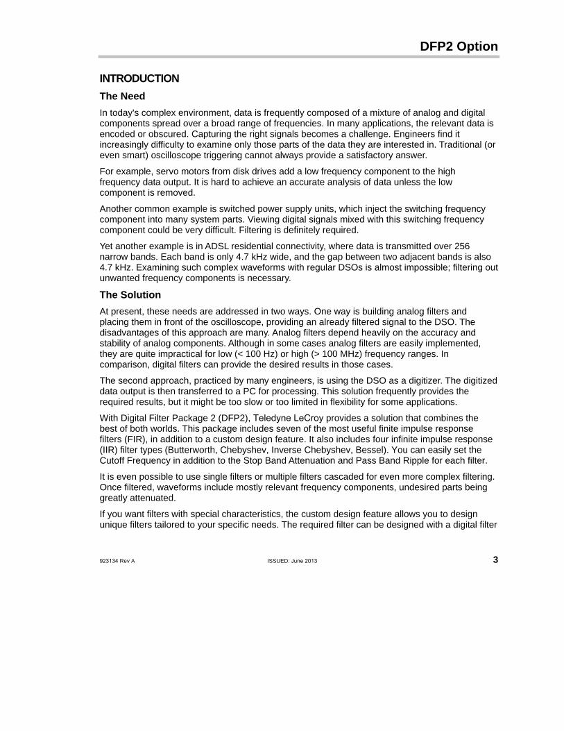
DFP2's flexibility is shown by the following example:

1. A 25 kHz square wave combinedwith an unwanted 60 Hz sinusoidal component.

2. A high-pass filter set to attenuatesignals lower than 1 kHz is applied to remove the unwanted 60 Hz component.

3. FFT of the unfiltered trace.

4. FFT of the filtered trace. Note theabsence of the 60 Hz component.

Enhanced Solutions DFP2 can be coupled with other Teledyne LeCroy software products such as JTA2 or DDM2 to enhance the capabilities of these products and to provide improved solutions. For Jitter Measurement, for example, the DFP2 Band-pass Filter can be coupled with the JTA2 package to measure jitter over a narrow frequency range.

DFP2 Option


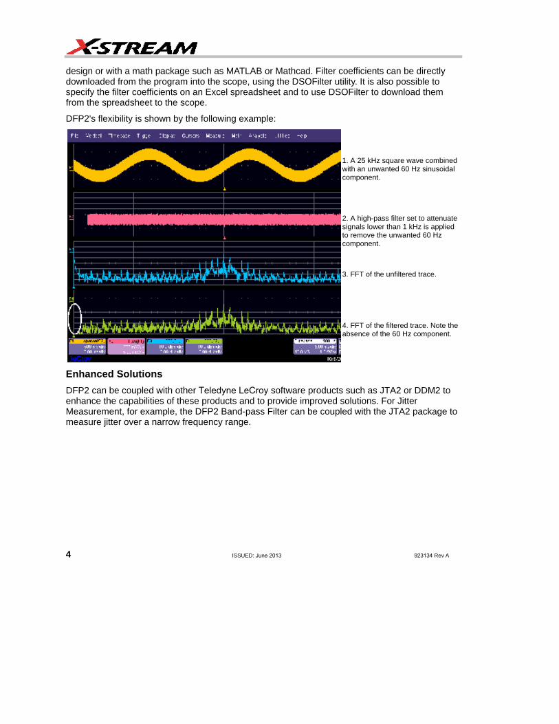
Kinds of Filters1

Low-pass Filter Low-pass filters are useful for eliminating accumulated high-frequency noise and interference, and for canceling high-frequency background noise.

Sample applications are in datacom, telecommunications, and disk drive and optical recording analysis for accurate RF signal detection.

Band 1: Pass Band — DC to top of the transition region; signal passes unattenuated.

Band 2: Transition Region — edge frequency to edge frequency plus width; increasing attenuation.

Band 3: Stop Band — above end of transition region; signal is highly attenuated.

High-pass Filter High-pass filters are useful for eliminating DC and low-frequency components. Sample applications include Disk Drive and Optical Recording analysis (emulation of the SLICING function).

Band 1: Stop Band — DC to bottom of the transition region; highly attenuated.

Band 2: Transition Region — edge frequency minus width to edge frequency; decreasing attenuation.

Band 3: Pass Band — above edge frequency; signal passes unattenuated.

1 1. Filters are optimal FIR filters of less than 2001 taps, according to the Parks-MacLellan algorithm described in Digital Filter Design and Implementation by Parks and Burrus, John Wiley & Sons, Inc., 1987, and then adjusted by windowing the start and end 20% with a raised cosine for improved time domain characteristics and better ultimate rejection in the frequency domain, slightly increasing 1st stop-band ripple height.


Band-pass Filter Band-pass filters are useful for emphasizing a selected frequency band. Sample applications include radio channel identification, broadband transmission, ADSL, clock generators (i.e., eliminating the central frequency and displaying harmonics only), and telecommunications (Jitter measurement over a selected frequency range).

Band 1: First Stop Band — DC to bottom of first transition region; highly attenuated.

Band 2: First Transition Region — lower corner minus width to lower corner; decreasing attenuation.

Band 3: Pass Band — signal passes unattenuated.

Band 4: Second Transition Region — upper corner to upper corner plus width; increasing attenuation.

Band 5: Second Stop Band — signal highly attenuated.

Band-stop Filter Band-stop filters are useful for eliminating a narrow band of frequencies. Sample applications include medical equipment, such as ECG monitors where the dominant ripple at 50/60 Hz is rejected, leaving the low energy biological signals intact. Digital troubleshooting: the inherent frequency of the switched power supply is blocked, revealing power line voltage drops and glitches caused by the system clock generator.

Band 1: First Pass Band — DC to bottom of first transition region; signal passes unattenuated.

Band 2: First Transition Region — lower corner minus width to lower corner; increasing attenuation.

Band 3: Stop Band — signal is highly attenuated.

Band 4: Second Transition Region — upper corner to upper corner plus width; decreasing attenuation.

Band 5: Second Pass Band — signal passes unattenuated.

DFP2 Option


Communications Channel Filters

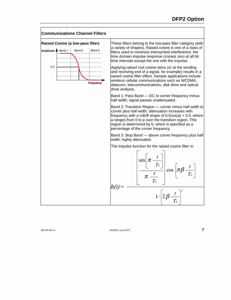
Raised Cosine (a low-pass filter) These filters belong to the low-pass filter category (with a variety of shapes). Raised cosine is one of a class of filters used to minimize intersymbol interference: the time domain impulse response crosses zero at all bit time intervals except the one with the impulse.

Applying raised root cosine twice (or at the sending and receiving end of a signal, for example) results in a raised cosine filter effect. Sample applications include wireless cellular communications such as WCDMA, datacom, telecommunications, disk drive and optical drive analysis.

Band 1: Pass Band — DC to corner frequency minus half width; signal passes unattenuated.

Band 2: Transition Region — corner minus half width to corner plus half width; attenuation increases with frequency with a rolloff shape of 0.5cos(a) + 0.5, where a ranges from 0 to p over the transition region. This region is determined by b, which is specified as a percentage of the corner frequency.

Band 3: Stop Band — above corner frequency plus half width; highly attenuated.

The impulse function for the raised cosine filter is:


Raised Root Cosine (a low-pass filter) Band 1: Pass Band — DC to corner frequency minus half width; signal passes unattenuated.

Band 2: Transition Region — corner minus half width to corner plus half width; attenuation increases with frequency with a rolloff shape of 0.5[cos(a) + 0.5]½, where a ranges from 0 to p over the transition region. This region is determined by b, which is specified as a percentage of the corner frequency.

Band 3: Stop Band: — above corner frequency plus half width; signal is highly attenuated.

The impulse function for the square-root raised cosine filter is:

Gaussian Band 1: Pass Band — DC to half power bandwidth% times modulation frequency, pass; 3 dB down at half power bandwidth.

The shape of a Gaussian filter’s frequency response is a Gaussian distribution centered at DC. The signal becomes more attenuated with increasing frequency. It is not possible to specify a transition region or a stop band for Gaussian filters. However, the BT value, a fraction of the symbol frequency, determines the filter’s width, where:

B = half power bandwidth

T = bit (or modulation period)

DFP2 Option


IIR Filters Infinite Impulse Response (IIR) filters are digital filters that emulate analog filters. The four types offered by the DFP2 option are as follows: • Butterworth• Chebyshev• Inverse Chebyshev• Bessel

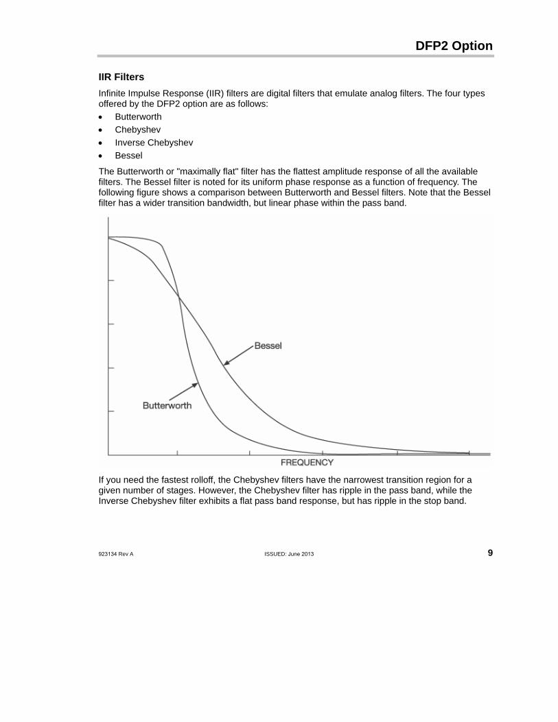
The Butterworth or "maximally flat" filter has the flattest amplitude response of all the available filters. The Bessel filter is noted for its uniform phase response as a function of frequency. The following figure shows a comparison between Butterworth and Bessel filters. Note that the Bessel filter has a wider transition bandwidth, but linear phase within the pass band.

If you need the fastest rolloff, the Chebyshev filters have the narrowest transition region for a given number of stages. However, the Chebyshev filter has ripple in the pass band, while the Inverse Chebyshev filter exhibits a flat pass band response, but has ripple in the stop band.


In the setup of these filters, you have control of cutoff frequencies, transition region width, and stop band attenuation.

FILTER SETUP To Set Up a DFP Filter 1. Touch Math in the menu bar then Math Setup... in the drop-down menu.

2. Touch the Fx tab (F1 for example) for the math trace you want to display your filtered waveform.

3. Touch the Single function button if you want to perform just one filtering function on

the trace, or touch the Dual function button to perform math on, or apply another filter to, the filter output.

4. Touch inside the Source1 field and select a source waveform from the pop-up menu.

5. Touch inside the Operaor1 field and select Filter from the pop-up menu. A mini-dialog to set up the filter will open at right.

Note: Other math choices in the Operator1 menu include Boxcar, ERES, and interpolation. The boxcar "filter" is a simple average taken over a user-specified number of points (the "length").

6. Touch inside the FIR/IIR field and select finite or infinite response filter FIR (non-recursive)filters require a limited number of multiplications, additions, and memory locations. On theother hand, IIR (recursive) filters, which are dependent on previous input or output values, intheory require an infinite number of each..

7. Whether you selected FIR or IIR, touch inside the Filter Kind field and select a filteringoperation. Some choices are not available for IIR.

8. If you selected FIR, touch inside the Type field and choose an FIR filter type. Then touchinside the Taps2 data entry field and enter a value, using the pop-up numeric keypad.Alternatively, you can touch the Auto Length checkbox; the Taps field is grayed out and thescope calculates the optimum number of coefficients. If you selected IIR, touch inside theType field and choose an IIR filter type. Then touch inside the Stages data entry field andenter a value, using the pop-up numeric keypad. Alternatively, you can touch the AutoLength checkbox; the Stages field is grayed out and the scope calculates the optimumnumber of stages.

2 The number of coefficients. The number of coefficients. The suggested number of taps is a minimal suggestion: using even more taps can give a more desirable response. Using less than the suggested number of taps will not meet the requested specifications.

DFP2 Option


9. Touch the Frequencies tab.10. Depending on the class (FIR/IIR) and kind of filter you selected, and whether or not Auto

Length is enabled, you can change the cutoff frequencies, transition width (edge width), stopband attenuation, and pass band ripple.

MULTIRATE FILTERS Description In many of today's development environments, digital filter design has become most challenging. Specifications typically require higher order filters, implying increased storage capacity for filter coefficients and higher processing power. Moreover, high-order filters can be difficult, if not impossible, to design. In applications such as 3G wireless systems, for example, at the receiver end data must be filtered very tightly in order to be processed.

Although the Teledyne LeCroy DFP option provides many filter types, the correlation between edge frequencies and sample rate may be a limiting factor: edge frequencies are limited from 1% to 49.5% of the sample rate, while the minimum transition width region is 1% of the sample rate.

Multirate, multistage filters are a practical solution for the design and implementation of FIR filters with narrow spectral constraints. Multirate filters change the input data rate at one or more intermediate points within the filter itself, while maintaining an output rate that is identical to the input rate. This approach provides a solution with greatly reduced filter lengths, as compared to standard single-rate filters.

This can be achieved in two or more simple steps. First, a filter (with a relatively limited edge frequency) is applied and the results are decimated. Then, a second filter is applied to the decimated waveform, substantially reducing the lower edge frequency limit.

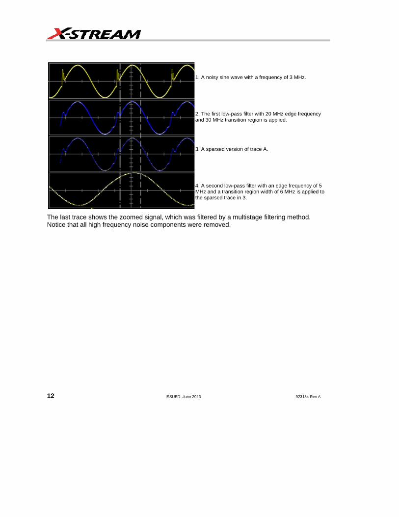
Example A sine wave with a frequency of 3 MHz has a higher frequency noise component. A low-pass filter is required to remove the noise component. The sample rate of the scope is 2 GS/s. The minimum edge frequency of the low-pass filter for this sample rate is 20 MHz. While this filter is sufficient for removing part of the noise, it cannot remove the high frequency component completely. In such a case, the problem can be solved in two stages.


1. A noisy sine wave with a frequency of 3 MHz.

2. The first low-pass filter with 20 MHz edge frequencyand 30 MHz transition region is applied.

3. A sparsed version of trace A.

4. A second low-pass filter with an edge frequency of 5MHz and a transition region width of 6 MHz is applied to the sparsed trace in 3.

The last trace shows the zoomed signal, which was filtered by a multistage filtering method. Notice that all high frequency noise components were removed.

DFP2 Option


CUSTOM FILTERS Custom Filter Setup If the standard filters provided with DFP2 are not sufficient for your needs, you can create filters with virtually any characteristic, up to 2000 taps.

The required custom filter can be designed with a digital filter design or math package such as MATLAB or Mathcad. The filter coefficients can then be loaded into the scope from an ASCII file. The file consists of numbers separated by spaces, tabs, or carriage returns. Note: Do not use commas as separators.

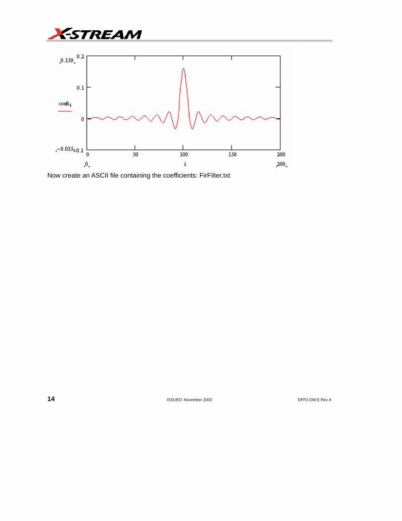
For a custom IIR filter there needs to be a multiple of 6. Each stage consists of 3 numbers for the numerator polynomial followed by 3 numbers for the denominator polynomial. They are in the order a b c where the polynomial is of the form: a + b * z-1 + c * z-2. Example 1: Creating an FIR Filter Coefficient File Using Mathcad N := 200 i := 0..N

sinx(x) := sin(x)/x

200 point sin(x)/x, a low-pass filter.

Note: Real world filters would either be windowed or made by the Remez exchange algorithm. The point of this example is to show how to transfer a filter to the scope.

check = 0.987 This is the DC gain of the filter

14 ISSUED: November 2003 DFP2-OM-E Rev A

Now create an ASCII file containing the coefficients: FirFilter.txt

DFP2 Option

DFP2-OM-E Rev A ISSUED: November 2003 15

Writing Data to a Data File To write values from Mathcad version 11 to a data file, you can use the File Read/Write component, as follows:

1. Click in the blank spot in your worksheet.

2. Choose Insert, Data, File Output from the menu.


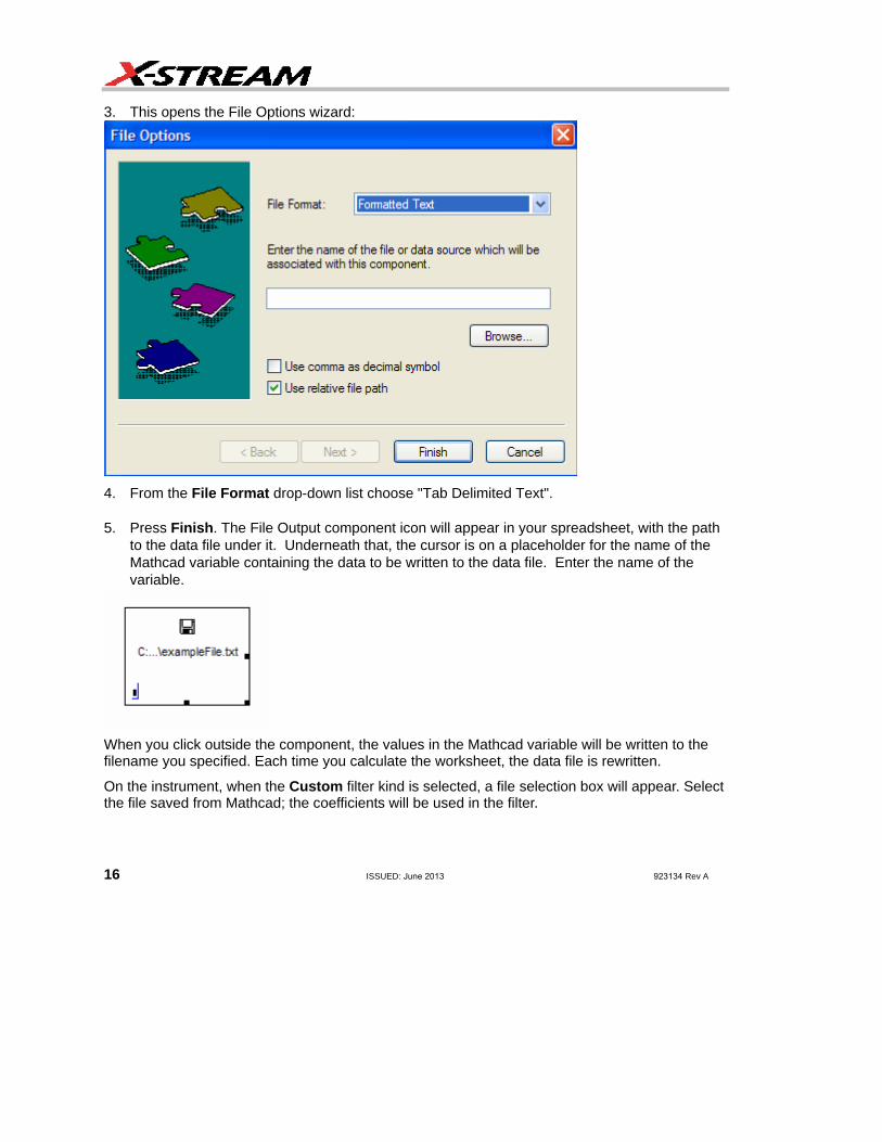
3. This opens the File Options wizard:

4. From the File Format drop-down list choose "Tab Delimited Text".

5. Press Finish. The File Output component icon will appear in your spreadsheet, with the pathto the data file under it. Underneath that, the cursor is on a placeholder for the name of theMathcad variable containing the data to be written to the data file. Enter the name of thevariable.

When you click outside the component, the values in the Mathcad variable will be written to the filename you specified. Each time you calculate the worksheet, the data file is rewritten.

On the instrument, when the Custom filter kind is selected, a file selection box will appear. Select the file saved from Mathcad; the coefficients will be used in the filter.

DFP2 Option

DFP2-OM-E Rev A ISSUED: November 2003 17

Example 2: Creating an IIR Filter Coefficient File Using Mathcad Note: This example uses the Mathcad Signal Processing Extension Pack. order 6:= fcutoff .1:= A iirlow butter order( ) fcutoff,( ):=

A

0.083

0.166

0.083

1

1.404−

0.736

0.067

0.135

0.067

1

1.143−

0.413

0.061

0.122

0.061

1

1.032−

0.276

⎛⎜⎜⎝

⎞

⎠=

x 0 .001, .5..:=

0 0.1 0.2 0.3 0.4 0.50

0.5

11

0

gain A x,( )

0.50 x

Now create an ASCII file containing the coefficients: IirFilter.txt

Note: The diskette icon, the file name, and the "A" below it are the representation of a Mathcad "File Output" component. It is inserted by selecting Insert, Data, File Output. You must specify the file name ("IirFilter.txt" in the example) and fill in the variable name that is the source of the data ("A" in the example). Be sure to specify a complete path for the file.


Note: In the example above, because “A” has a predefined meaning (as a unit) in Mathcad 11, it appears with a green underline. However, earlier versions of Mathcad give no warning about using "A" as a variable name, and it may still be used for this purpose.

What gets written to lirfilter.txt is as follows: 0.0828825751812225 1 0.0674552738890719 1 0.0609096342883086 1

0.165765150362445 -1.40438489047158 0.134910547778144 -1.1429805025399 0.121819268576617 -1.03206940531971

0.0828825751812225 0.735915191196472 0.0674552738890719 0.412801598096189 0.0609096342883086 0.275707942472944

DFP2 Option


Writing Data to a Data File To write values from Mathcad to a data file, you can use the File Read/Write component, as follows: 1. Click in the blank spot in your worksheet.2. Choose Component from the Insert menu.3. Select File Read or Write from the list and click Next. This launches the first part of the File

Read or Write Setup Wizard.4. Choose Write to a data source and press Next to go to the second page of the Wizard:

From the File Format drop-down list in this Wizard, choose Tab Delimited Text.5. Type the path to the data file you want to write, or click the Browse button to locate it.6. Press Finish. You'll see the File Read or Write component icon and the path to the data file.

In the place holder that appears at the bottom of the component, enter the transposed nameof the Mathcad variable containing the data that will be written to the data file. It is importantto transpose the variable (Ctl + 1) so that the variables appear in the correct order.

When you click outside the component, the values in the Mathcad variable will be written to the filename you specified. Each time you calculate the worksheet, the data file is rewritten.

On the instrument, when the Custom filter kind is selected, a file selection box will appear. Select the file saved from Mathcad; the coefficients will be used in the filter.

SPECIFICATIONS • The pass-band gain of all filters (except custom) is normalized to 1.• FIR Coefficients: 2001 max.• IIR Stages: 29 max.• Filter Kinds: high pass, low pass, band pass, band stop, raised cosine, raised-root cosine,

Gaussian, custom• IIR Filter Types: Butterworth, Chebyshev, Inverse Chebyshev, Bessel

§ § §

DFP2 Software Instruction Manual

Documents

Transcript of DFP2 Software Instruction Manual