A Two-Factor Cointegrated Commodity Price Model with … ANNUAL MEETINGS/2015-… · A Two-Factor...

A Two-Factor Cointegrated Commodity Price Model with an

Application to Spread Option Pricing∗

Walter Farkas ‖§ Elise Gourier ∗∗ Robert Huitema Ciprian Necula ‡‡

January 15, 2015

Abstract

We introduce a flexible continuous-time model of cointegrated commodity prices, which

allows capturing between one and n−1 cointegration relations between the n components

of a system. Closed-form expressions for futures and European option prices are derived.

The model is estimated using futures prices of ten commodities. We find compelling

evidence of multiple cointegration relationships. We calculate the prices of options

written on various spreads such as the spark spread and the crack spread. We show

that cointegration creates an upward sloping term structure of correlation, which lowers

the volatility of spreads and consequently the price of options on them.

Keywords: Commodities, Cointegration, Futures, Option Pricing, Spread Options, Spark

Spread, Crack Spread

JEL classification: C61, G11, G12

∗We thank the staff from the trading and risk management divisions of AXPO AG for useful discussions

and sharing data.University of Zurich, Department of Banking and Finance, Plattenstrasse 14, 8032 Zurich, Switzerland‖ETH Zurich, Department of Mathematics, Ramistrasse 101, 8092 Zurich, Switzerland§Corresponding author, Email: [email protected]∗∗Princeton University, ORFE, Princeton, USA‡‡Bucharest University of Economic Studies, Department of Money and Banking, Bucharest, Romania

mailto:[email protected]

2

One of the most distinctive features of commodity markets is the large number of long-

run equilibrium relationships that exist between certain commodity prices. For example,

the price of crude oil may move against the price of heating oil on a given day but not in

the long run. That is in the long-run, the price of crude oil is tied to the price of heating

oil in an equilibrium relation. These long-run equilibrium relations are usually referred to

as cointegration relations. Cointegrated systems set in discrete time are widely employed

in economics, especially empirical macroeconomics, to analyze various phenomena. Engle

and Granger (1987) and Johansen (1991) revolutionized the field by a series of seminal

results, such as the Granger representation theorem stating that a cointegrated system set

in discrete time has an autoregressive error correction model (ECM) representation. Similar

results are available for continuous time systems, but modeling cointegration in continuous

time is less popular in economics. Phillips (1991) introduced the concept of cointegartion in

continuous time modeling and pointed out that the long-run parameters of a continuous time

model can be estimated from discrete data by focusing on the corresponding discrete time

ECM. Comte (1999) models cointegration in a continuous-time framework using CARMA

(continuous-time autoregressive moving average) processes and develop a continuous time

Granger representation theorem.

In this paper we develop a continuous time model of cointegrated commodity prices. This

model features non-stationary commodity prices that are allowed be cointegrated. There is a

vast literature on modelling the price of a single commodity as a non-stationary process. For

example, Schwartz and Smith (2000) assume the log price to be the sum of two latent factors:

the long-term equilibrium level, modeled as a geometric Brownian motion, and a short-term

deviation from the equilibrium, modeled as a zero mean Ornstein - Uhlenbeck (OU) process.

To account for higher order autoregressive and moving average components in the short-run

deviation from equilibrium, Paschke and Prokopczuk (2010) propose to model these deviations

as a more general CARMA process. Moreover, Cortazar and Naranjo (2006) generalizes the

Schwartz and Smith (2000) model in a multi-factor framework. For an extensive account of

the various types of one dimensional commodity price models, the reader is referred to the

recent review of Back and Prokopczuk (2013). However, the literature on modeling a system

of commodity prices is quite scarce.

Although cointegration has been studied well from a statistical and an econometric point of

view, see e.g., Baillie and Myers (1991), Crowder and Hamed (1993) and Brenner and Kroner

(1995), it has received little attention in the continuous-time asset pricing literature. Two

fairly recent models, which are closly related to the one developed in this paper, are proposed

3

in Cortazar et al. (2008) and Paschke and Prokopczuk (2009), both of which account for

cointegration by incorporating common and commodity-specific factors into their modeling

framework. Amongst the common factors, only one is assumed non-stationary. Although they

take into account explicitly that prices are cointegrated, the cointegrated sytems generated

by these two models are not covering the whole range of possible number of contegration

relations, but allow for none or for exactly n− 1 relations to exist between the n prices.

Research on the pricing of derivatives written on cointegrated assets is understandably

even scarcer. Duan and Pliska (2004) were (to the best of our knowledge) the first to examine

the implications of cointegration for derivatives prices. They use a cointegrated multi-variate

GARCH model to price options on the spread between two stocks. Their findings indicate that

these prices only depend on the presence of cointegration when volatilities are stochastic. The

recent paper by Nakajima and Ohashi (2012) also focuses on the implications of cointegration

on spread options, but in contrast to Duan and Pliska (2004), they consider commodity rather

than equity spread options. Their modeling approach is also somewhat different from Duan

and Pliska (2004). Nakajima and Ohashi (2012) write the continuous-time model of Gibson

and Schwartz (1990) down in a multi-variate cointegration framework. More specifically,

they assume that the risk-neutral drift of a commodity spot log-price temporarily deviates

from the risk-free rate, and that these deviations are described by convenience yields and

cointegrating relations among the prices. Their primary finding is that – unlike the result

of Duan and Pliska (2004) – cointegration affects the prices of commodity spread options

no matter whether volatility is stochastic or not. This discrepancy in the findings of Duan

and Pliska (2004) and Nakajima and Ohashi (2012) is due to the fact that stocks (unlike

commodities) earn the risk-free rate under the pricing (or risk-neutral) measure.

Dempster et al. (2008) argue that when a cointegration relationship exists between two

asset prices only the spread between the two should be modeled. This approach has the

advantage that closed-form analytic pricing formulae for spread options may exist depending

on the complexity of the dynamics. Dempster et al. (2008) obtain closed-form solutions under

a two-factor Ornstein-Uhlenbeck (OU) process for the dynamics of the spot spread. However,

this “direct” approach also presents certain drawbacks: since only the spread is modeled, it

is not possible to obtain prices for futures and options on the individual components of the

spread, nor is it possible to use market data on these derivatives. Furthermore, it is not

straightforward to formulate the dynamics of the spread because it may, for example, reach

negative values, but certainly not large negative values. An OU or square-root process would

then not be appropriate choices.

4

To avoid these disadvantages, we follow Duan and Pliska (2004) and Nakajima and

Ohashi (2012), among others, and model the dynamics of the (underlying) assets forming

the spread. More specifically, we extend the modelling framework developed by Schwartz

and Smith (2000). These two authors model the spot price dynamics of one commodity

with two factors and show that their model is equivalent to the stochastic convenience-

yield (SCY) model proposed by Gibson and Schwartz (1990). They do argue, however, that

their specification better conforms with intuition than models based on the somewhat elusive

notion of “convenience yield”. Our extension of the Schwartz and Smith (2000) model to n

commodities is parsimonious and intuitive. Just like Schwartz and Smith (2000), we use two

factors to model the dynamics of the spot price of each commodity. Then, we assume that

both factors are correlated across the n commodities, and that the long-term factor is also

cointegrated across the n commodities. In contrast to the models mentioned above, our model

can deal with one up to n − 1 cointegration relationships, instead of only one (cf. Nakajima

and Ohashi (2012)) or precisely n − 1 (cf. Paschke and Prokopczuk (2009)). Furthermore,

we argue that the idea of a cointegrated long-term (equilibrium) factor is more natural and

intuitive than cointegrated convenience yields (cf. Duan and Pliska (2004), Cortazar et al.

(2008)).

The model is estimated utilising data of futures prices for crude oil, heating oil, gasoline,

natural gas and electric power. Compelling evidence is found of multiple cointegration

relationships. For example, our results indicate that two cointegration relationships exist

between crude oil, heating oil, gasoline and natural gas. Furthermore, we find evidence for

cointegration between natural gas and electric power, and between electric power in various

markets. To gain a better understanding of our model and of its implications for futures and

spread options, we calculate the prices of futures and options written on the spark spread,

the crack spread and on a spread between electric power prices in different markets, using

the results of our model estimation. The results give a clear and concise overview of the

implications of cointegration in commodity markets. Confirming previous work (cf., e.g.,

Nakajima and Ohashi (2012)), we find that cointegration alters the shape of term-structures

of futures prices at long horizons. Furthermore, we find that cointegration creates an upward-

sloping correlation term-structure. The latter finding is consistent with empirical evidence,

but more importantly, it lowers the volatility of spreads, lowering therefore the prices of spread

options.

The rest of the paper is organized as follows. In Section 1, we present the details of the

model. Section 2 is devoted to deriving closed-form pricing formulae for futures and European-

5

style options. In Section 3, we estimate the model using data of futures prices for ten energy

commodities. The purpose of Section 4 is to demonstrate the effects of cointegration on

futures prices and spread option prices. Section 5 concludes.

1 Model for commodity spot prices

The model is constructed in such a way that it allows for several cointegration relations

among the two factors driving the commodity prices in the system. The model also allows

for obtaining closed-form prices of futures and European-style options. First, we start with a

brief discussion of what the concept of cointegration entails.

Cointegration

Cointegration is a time-series property which was introduced by Engle and Granger (1987).

Cointegration exists when a linear combination of two or more non-stationary time-series is

stationary. To explain this by an example, let us suppose that X1(t) and X2(t) (where t

denotes time) are two variables, then the time-series X1(t)t∈T and X2(t)t∈T (where T

denotes a set of discrete time steps) are said to be cointegrated, when both are non-stationary,

but a linear combination of them, say, X1(t)− αX2(t)t∈T , is stationary for some α ∈ R>0.

In simply words, cointegration occurs when the paths of two or more variables (e.g. a pair or

pool of stocks, interest rates or commodity futures) are linked to form a long-run equilibrium

relationship from which they only temporarily depart.

Spot price model

Let (Ω,F , Ftt≥0,P) be a filtered probability space satisfying the usual assumptions,

where P denotes the statistical measure. We consider n commodity spot prices S(t) =

(S1(t), . . . , Sn(t))> and denoteX(t) = logS(t). Let X(t) = X(t)−φ(t) be the de-seasonalized

log price process. Following Sorensen (2002), Paschke and Prokopczuk (2009), Nakajima and

Ohashi (2012), the function φ(t) is defined as follows:

φ(t) = χ1 cos(2πt) + χ2 sin(2πt), (1)

6

where χ1 and χ2 are n-dimensional vectors of constants.1 The process X(t) is assumed to

mean-revert towards a stochastic (non-stationary) long-run level Y (t), as specified by the

following system of stochastic differential equations:

d

X(t)

Y (t)

=

−Kx(X(t)− Y (t))

µy −KyΘY (t)

dt+

Σ12x On

Σ12xy Σ

12y

dW x(t)

W y(t)

(2)

where On refers to the matrix of size n × n full of zeros and W := (W x,W y)> is a 2n-

dimensional standard Brownian motion. Let us stress that there are n natural cointegration

relationships assumed by equation (2): the n seasonally adjusted spot log-prices X(t) are

cointegrated with the corresponding elements of Y (t). The matrix Kx is an n×n matrix that

quantifies the speed of mean reversion of the elements in X towards the long term levels in

Y . Note that the matrix Kx need not be diagonal. Intuitively we think of the two factors,

X and Y , as the short-end and the long-end of the term-structure of futures prices.

The main feature of our model is that it allows cointegration between the variables in

Y (t). We denote the number of cointegration relationships between them by h, where h ≥ 0

and h < n. The cointegration matrix Θ is an n × n matrix of rank h. Its last n − h rows

contain only zeros. Each of the h non-zero rows of Θ encodes a stationary (i.e., cointegrating)

combination of the variables in Y (t), normalized such that Θii = 1, i ≤ h. The matrix Ky is

a n×n matrix with the last n−h columns filled with zeros, such that KyΘ is a n×n matrix

of rank h. Each of the h non-zero columns in Ky represents the speed of adjustment of each

element in Y towards the corresponding cointegration relation.

Let us denote Z(t) = (X(t)−φ(t),Y (t))>. The n+h cointegration relationships between

the variables in the 2n-dimensional vector Z(t) can be characterized by the following (2n×2n)

cointegration matrix In −InOn Θ

(3)

1The seasonal behavior of energy commodity prices is documented, among others, by Manoliu and Tompaidis(2002), Borovkova and Geman (2006), Geman and Ohana (2009). As pointed out by Back et al. (2013), adeterministic seasonal component is not relevant for the pricing of commodity futures options, given observedfutures prices. However, as noted by Lo and Wang (1995) and Back et al. (2013), a deterministic component inthe price process might have a significant impact on the estimation of the model parameters, and, thereofore,indirectly on option prices.

7

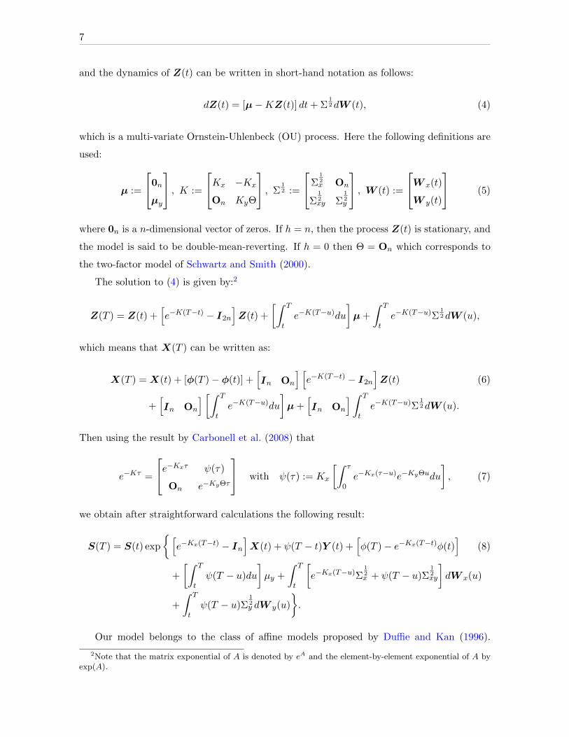
and the dynamics of Z(t) can be written in short-hand notation as follows:

dZ(t) = [µ−KZ(t)] dt+ Σ12dW (t), (4)

which is a multi-variate Ornstein-Uhlenbeck (OU) process. Here the following definitions are

used:

µ :=

0nµy

, K :=

Kx −Kx

On KyΘ

, Σ12 :=

Σ12x On

Σ12xy Σ

12y

, W (t) :=

W x(t)

W y(t)

(5)

where 0n is a n-dimensional vector of zeros. If h = n, then the process Z(t) is stationary, and

the model is said to be double-mean-reverting. If h = 0 then Θ = On which corresponds to

the two-factor model of Schwartz and Smith (2000).

The solution to (4) is given by:2

Z(T ) = Z(t) +[e−K(T−t) − I2n

]Z(t) +

[∫ T

te−K(T−u)du

]µ+

∫ T

te−K(T−u)Σ

12dW (u),

which means that X(T ) can be written as:

X(T ) = X(t) + [φ(T )− φ(t)] +[In On

] [e−K(T−t) − I2n

]Z(t) (6)

+[In On

] [∫ T

te−K(T−u)du

]µ+

[In On

] ∫ T

te−K(T−u)Σ

12dW (u).

Then using the result by Carbonell et al. (2008) that

e−Kτ =

e−Kxτ ψ(τ)

On e−KyΘτ

with ψ(τ) := Kx

[∫ τ

0e−Kx(τ−u)e−KyΘudu

], (7)

we obtain after straightforward calculations the following result:

S(T ) = S(t) exp

[e−Kx(T−t) − In

]X(t) + ψ(T − t)Y (t) +

[φ(T )− e−Kx(T−t)φ(t)

](8)

+

[∫ T

tψ(T − u)du

]µy +

∫ T

t

[e−Kx(T−u)Σ

12x + ψ(T − u)Σ

12xy

]dW x(u)

+

∫ T

tψ(T − u)Σ

12y dW y(u)

.

Our model belongs to the class of affine models proposed by Duffie and Kan (1996).

2Note that the matrix exponential of A is denoted by eA and the element-by-element exponential of A byexp(A).

8

Therefore, the futures prices are exponentially affine in the two factors and the prices of

European-style options are still given by a Black-like formula (see Black (1976)), which enables

fast and efficient computations. The characteristic function of X(t) can be readily computed

analytically, as shown in Lemma 1 in Appendix A.

Finally, we would like to stress that adding jumps by specifying a mean-reverting jump-

diffusion process for X(t) (as in e.g. Hambly et al. (2009)) would not lead to other conclusions

with respect to the effects of cointegration. The reason is that spot price jumps typically have

a strong tendency to “mean-revert” (Hambly et al. (2009) find a jump mean-reversion rate

that is many times higher than that of the purely diffusive part of X(t)) and therefore only

affect short-dated option prices, in contrast to cointegration which affects, essentially, only

long-dated option prices.

2 Pricing of futures and European options

As there is no traded instrument that allows hedging the risks driving the components of the

stochastic level of reversion vector Y , the market is incomplete and the risk-neutral measure

not unique. We parameterize the pricing kernel so that the market prices of risk be constant.

The corresponding risk-neutral measure, equivalent to P, is denoted by Q. The dynamics of

Z(t) under Q become:

dZ(t) = [µ∗ −KZ(t)] dt+ Σ12dW ∗(t), (9)

where W ∗(t) :=

W ∗x(t)

W ∗y(t)

, W ∗x(t) and W ∗

y(t) are Q - Brownian motions, µ∗ =

µ∗xµ∗y

=

µ− Σ12

λxλy

and λx, λy are the market prices of the two sources of risk.

We now readily obtain Proposition 1, which gives the “fair value” of a futures contract

under the model.

Proposition 1. At time t the price of a futures contract with maturity T is given by

F (t, T ) = exp α(t, T ) + β(T − t)X(t) + γ(T − t)Y (t) , (10)

9

with β(τ) := e−Kxτ , γ(τ) := ψ(τ) and with α(t, T ) defined by

α(t, t+ τ) :=[φ(t+ τ)− e−Kxτφ(t)

]+(In − e−Kxτ

)K−1x µ∗x +

(∫ τ

0ψ(τ − u)du

)µ∗y (11)

+ diag

1

2

[In On

] [e−Kτ

(∫ τ

0eKuΣeKudu

)e−Kτ

]InOn

,where diag(A) returns the vector with diagonal elements of A.

Proof. See Appendix B. q.e.d.

From Proposition (1), we see that the futures price F (t, T ) is an exponential affine function

of the two factors X(t) and Y (t). Note that, while the coefficients β and γ only depend on

time t and maturity T through the (remaining) time to maturity T − t, α depends on both

variables t and T independently (due to the seasonality function φ(t)).

By Ito’s lemma the risk-neutral dynamics of F (t, T ) are given by

dF (t, T )

F (t, T )=

[e−Kx(T−t)Σ

12x + ψ(T − t)Σ

12xy

]dW ∗

x(t) + ψ(T − t)Σ12y dW

∗y(t), (12)

which immediately gives us the next proposition.

Proposition 2. The variance-covariance matrix of returns on futures prices is given by:

Ξ(τ) = e−KxτΣxe−K>x τ + ψ(τ)Σ

12xy(Σ

12x )>e−K

>x τ + e−KxτΣ

12x (Σ

12xy)>ψ>(τ) (13)

+ ψ(τ)Σxyψ>(τ) + ψ(τ)Σyψ

>(τ)

Proof. Follows immediately from (12). q.e.d.

Proposition 2 shows that unless Kx = On, the variance-covariance matrix Ξ(τ) depends

on τ .

Given that returns on futures prices follow a pure-diffusion process one can also readily

obtain closed-form pricing formulae for plain vanilla options of European style. These formulae

are given in Proposition 3 below.

Proposition 3. The time-t price of a European-style call option with strike k and maturity

T is given by

c(t, F (t, T ), k, T, v(t, T ), r(t, T )) = e−r(t,T )(T−t) [F (t, T )N(d1)−KN(d2)] , (14)

10

where r(t, T ) is the risk-free rate for maturity T . The parameters d1,2 are given as usual by

d1,2 =log(F (t, T )/K)± 1

2v2(t, T )(T − t)

v(t, T )√T − t

, (15)

where v(t, T ) in turn is given by

v(t, T ) =

√1

T − t

∫ T

tΞ(T − s)ds. (16)

Proof. This is Black’s formula (see Black (1976)). q.e.d.

3 Estimation results

The model is estimated on three sets of data. Data set I consists of weekly time-series data

on the closing futures prices of 4 closely linked energy commodities, namely crude oil, heating

oil, gasoline3 and natural gas.4 The contracts have maturities of 1, 3, 6, 9 and 12 months and

are listed and traded on the NYMEX (New York Mercantile Exchange). The data span the

period from January 1991 to December 2013.

Data set II is composed of weekly time-series data on the closing futures prices of electric

power in 4 different markets, namely Germany, Nordics,5 Switzerland and Poland.6 These

data cover a relatively short time period from January 2007 to December 2013.

Typically the most liquid and high-volume electric power futures contracts are the so-called

Base Month, Base Quarter and Base Year ones. The Base Month is a contract delivering 720

MWh (megawatt-hours) for a period of 1 month (1MW × 30 days × 24 h/day = 720MWh).

Base Quarter (Year) contracts are nothing else than a series of 3 (12) consecutive Base Month

contracts.

To make the model compatible with the data in set II we regard 720 MWh electric power

for a period of 1 month as a commodity, and we shall henceforth refer to it as the power

commodity. Note that we have 4 power commodities, one for each region. The power

commodity serves as the underlying asset for the Base Month contract. The theoretical (or

model) futures prices of the Base Month contract can be easily calculated by using (10). The

3From January 1991 to December 2005 data on Unleaded Gasoline (HU) is used, while data on ReformulatedBlendstock for Oxygenate Blending (RB) is used for the remainder of the period (i.e., for the period January1996 to December 2013). The reason is that the HU contracts stopped trading on NYMEX end of 2005.We note that the HU and RB contracts were trading at almost the same prices over the 2-year period theyco-existed.

4This data set was retrieved from Quandl (www.quandl.com).5The Nordics consist of Sweden, Norway, Denmark, Finland, Iceland, The Faroe Island and Greenland.6This data set was obtained from the trading division of AXPO AG.

11

Base Quarter contract is, as noted earlier, a bundle of 3 Base Month contracts with maturities

T , T + 1M and T + 2M (capital “M” means month). Similarly, the Base Year contract with

maturity T is a bundle of 12 Base Month contracts with maturities T , T + 1M , . . ., T + 10M

and T + 11M . It follows therefore that the price of a Base Quarter (Base Year) contract is

simply given by the average of the prices of 3 (12) Base Month contracts. For each type of

contract (i.e., Base Month, Base Quarter and Base Year), we only use the data on the nearest

futures contracts. The reason is that on some days and for some regions only one maturity is

available.

Data set III comprises weekly time-series data on the closing prices of electric power

(Phelix Base Futures) and natural gas (TTF Natural Gas Futures) futures contracts, both

of which are traded on the EEX (European Energy Exchange).6 The data cover the time

period from January 2006 to December 2013. The reason for not taking the weekly natural

gas futures prices from data set I and/or the weekly electric power futures prices from data set

II is simply because these data cannot be (straightforwardly) used to compute values of the

spark spread (which is defined as the spread between the market price of electric power and

the cost of the natural gas needed to produce that electric power). The “power commodity”

in data set III corresponds to electric power for one day and the “natural gas commodity”

corresponds precisely to the amount of natural gas needed to generate that much electricity,

which enables an easy calculation of the spark spread.

Since the state variables X(t) and Y (t) cannot be observed directly from the data, they

must be inferred from the (observable) futures prices. We use the Kalman filter for this

purpose.7 The state (or transition) equation is given by (2). The measurement equation is

obtained by adding a n-dimensional (uncorrelated) Gaussian noise term to the right-hand side

of (10). We stress that the Kalman filter is applicable because the transition and measurement

equation are subject to Gaussian noise and linear in X(t) and Y (t). The Kalman filter is also

used for computing the likelihood of the (observed) futures prices given the model and the

model parameters. This facilitates a straightforward maximum likelihood (ML) estimation of

the model parameters.

Given that there are a large number of parameters, we employ a two-step ML estimation

procedure. In the first step, we estimate a simple one-dimensional version of the model for

each commodity separately. The estimates for the parameters of the seasonality term (1),

as well as those for the variance of the measurement errors, are kept fixed in the second

step. The estimates for the other parameters serve as starting point for the second step of

7We refer the reader to Kalman (1960) or Welch and Bishop (1995) for more details about the Kalmanfilter.

12

the estimation procedure. The filtered values of the latent state variables X(t) and Y (t)

are utilized to calculate reasonable starting values for parameters that cannot be estimated

within the model version used in step one (i.e., correlation and cointegration parameters).

In the second step of the estimation procedure, the parameters of the full model are

estimated (with exception of those that are kept fixed at values obtained in the first step).

This time the log-likelihood function is maximized under the restriction that the model is

“well-specified”. Specifically, this means that at each iteration (of our maximization routine)

we perform a Johansen constraint test,8 checking whether the cointegration properties of the

filtered time-series of X(t) and Y (t) do not contradict with the cointegration matrix Θ.

From now onwards we present and discuss the estimation results. Figures 17 through

26 (Appendix C) show the time-series of the spot log-prices X(t) and the long-run log-price

levels Y (t), both of which were filtered from the data. For all 10 commodities, we observe

that the spot log-prices X(t) fluctuate quite wildly around the long-run log-price levels Y (t),

which themselves are also varying over time (but with a lower magnitude, as expected). The

bottom panels (of Figures 17 through 26) depict the seasonality patterns we found in the data.

We note from these results that there is a very noticeable seasonality in the (futures) prices

of heating oil, gasoline and the 4 power commodities with the exception of “power Poland”.

The seasonality seen in crude oil prices seems negligible.

For comparison reasons, the 10 long-run log-price levels Y (t) are also shown in Figures 1

through 3. Figure 1 suggests that the long-run log-price levels of crude oil, heating oil and

gasoline are driven by only one factor. This would mean that no less than 2 cointegration

relationships exist among these 3 variables. The long-run log-price level of natural gas,

however, seems to be driven by another factor. These visual findings are confirmed by the

estimated cointegration matrix (see (17)), denoted by ΘI for data set I, by ΘII for data set

II, and by ΘIII for data set III.9

8The Johansen test (see Johansen (1991)) is a procedure for testing the presence of cointegrationrelationships between two or more time-series.

9Statistical significance at 1% symbolized by ***, statistical significance at 5% symbolized by ** and statisticalsignificance at 10% symbolized by *

13

ΘI =

1.00 −0.69*** −0.28*** 0.03***

0.36*** 1.00 −1.47*** 0.05

0.00 0.00 0.00 0.00

0.00 0.00 0.00 0.00

, ΘII =

1.00 −1.33*** 0.00 0.00

0.00 1.00 −0.63*** 0.00

0.00 0.00 1.00 −0.74***

0.00 0.00 0.00 0.00

,(17)

ΘIII =

1.00 −2.27***

0.00 0.00

.It is clear from Figure 2 that the long-run log-price levels of power in the 4 regions are driven

by only one factor. Intuitively this also makes sense because one would expect that price

differences between regions (or countries) stabilize in the long-run. This visual finding is also

confirmed by the estimated cointegration matrix ΘII .

1991 1992 1993 1994 1995 1996 1997 1998 1999 2000 2001 2002 2003 2004 2005 2006 2007 2008 2009 2010 2011 2012 2013 2014−2

0

2

4

6

Figure 1. Filtered time-series of the long-run log-price levels Y (t) (data set I). The colors correspondsto the following 4 commodities: gray (crude oil), red (heating oil), blue (gasoline), and green (naturalgas).

2007 2008 2009 2010 2011 2012 2013 20143

3.5

4

4.5

Figure 2. Filtered time-series of the long-run log-price levels Y (t) (data set II). The colors correspondsto the following 4 commodities: gray (power Germany), red (power Nordics), blue (power Swiss), andgreen (power Poland).

2006 2007 2008 2009 2010 2011 2012 2013 20142

2.5

3

3.5

4

4.5

Figure 3. Filtered time-series of the long-run log-price levels Y (t) (data set III). The colorscorresponds to the following 2 commodities: gray (electric power) and red (natural gas).

For the sake of completeness, we also report the estimates of the parameters other than

14

Θ. Values of these estimates can be found in Appendix C. Most of these results are well-

known, and are hence not covered in detail here. We only mention a few results that we find

interesting.

Recall that the matrices Kx and Ky measure the speed at which X(t) and Y (t) return to

their co-integrated equilibria. From the estimates of Kx and Ky, we see that X(t) returns at

least twice as fast to its equilibrium state than Y (t). This is a very intuitive result, because a

deviation of X(t) from its “equilibrium” value is likely due to daily fluctuations in supply and

demand (or speculative activity) whereas a deviation of Y (t) from its “equilibrium” value is

more likely due to structural shifts in supply and demand.

A second observation is that X(t) and Y (t) are strongly positively correlated, as indicated

by the estimates of Σxy. This result is again very intuitive if we recall that X(t) and Y (t)

correspond to the short-end and the long-end of the term-structure of futures prices, which

typically have a strong tendency to co-move (as evidenced by many empirical studies).

Finally, the fact that the elements of λy are, in general, positive proves that the risks

associated with changes in the Y (t)’s are priced. The values of the λx’s give a mixed result.

This means that investing in long-term futures contracts provides an extra return (in excess

of the risk-free rate) to compensate for the risks involved, but the same might not be true for

short-term futures contracts.

4 Prices for spread options

In this section we derive prices of European-style options written on the price difference,

or spread , between two or more commodities. Spread options present an ideal setting for

investigating the implications of cointegration, since they crucially depend on the short- and

long-run relation between the assets that make up the spread. Also, since spread options have

become regularly and widely-used instruments in financial markets for e.g. hedging purposes

or for exploiting (statistical) arbitrage opportunities, there is a growing need for a better

understanding of the effects of cointegration on their prices.

We will distinguish between options on spreads between 2 commodities and options on

spreads between n > 2 commodities. The reason is that for the 2-commodity case we have

analytic (approximation) formulas, such as Margrabe’s formula (see Margrabe (1978)) and

Kirk’s (approximation) formula (see Kirk (1995)), while for the general case (i.e., when n > 2)

we have to rely on numerical methods.10

10Also for the n = 3 case there are some (semi-)analytic approximation formulas, such as the extension ofKirk’s formula proposed by Alos et al. (2011), but here we give preference to the Monte-Carlo technique.

15

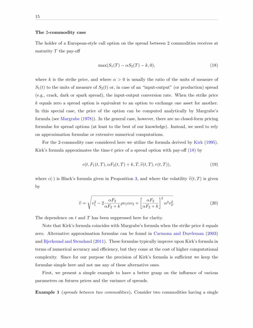
The 2-commodity case

The holder of a European-style call option on the spread between 2 commodities receives at

maturity T the pay-off

max(S1(T )− αS2(T )− k, 0), (18)

where k is the strike price, and where α > 0 is usually the ratio of the units of measure of

S1(t) to the units of measure of S2(t) or, in case of an “input-output” (or production) spread

(e.g., crack, dark or spark spread), the input-output conversion rate. When the strike price

k equals zero a spread option is equivalent to an option to exchange one asset for another.

In this special case, the price of the option can be computed analytically by Margrabe’s

formula (see Margrabe (1978)). In the general case, however, there are no closed-form pricing

formulae for spread options (at least to the best of our knowledge). Instead, we need to rely

on approximation formulae or extensive numerical computations.

For the 2-commodity case considered here we utilize the formula derived by Kirk (1995).

Kirk’s formula approximates the time-t price of a spread option with pay-off (18) by

c(t, F1(t, T ), αF2(t, T ) + k, T, v(t, T ), r(t, T )), (19)

where c(·) is Black’s formula given in Proposition 3, and where the volatility v(t, T ) is given

by

v =

√v2

1 − 2αF2

αF2 + kρv1αv2 +

[αF2

αF2 + k

]2

α2v22. (20)

The dependence on t and T has been suppressed here for clarity.

Note that Kirk’s formula coincides with Margrabe’s formula when the strike price k equals

zero. Alternative approximation formulae can be found in Carmona and Durrleman (2003)

and Bjerksund and Stensland (2011). These formulae typically improve upon Kirk’s formula in

terms of numerical accuracy and efficiency, but they come at the cost of higher computational

complexity. Since for our purpose the precision of Kirk’s formula is sufficient we keep the

formulae simple here and not use any of these alternative ones.

First, we present a simple example to have a better grasp on the influence of various

parameters on futures prices and the variance of spreads.

Example 1 (spreads between two commodities). Consider two commodities having a single

16

cointegration relation between their long term components given by Y1 − θY2 with θ > 0

and E[Y1 − θY2] = 0. Therefore, the cointegration matrix is Θ =

1 −θ

0 0

. We also assume

a simple specification for the dynamics given by χ1 = χ2 = 02, µy = 02, λx = λy =

02, Kx =

k1 0

0 k2

,with k1, k2 > 0,Ky =

l1 0

−l2 0

,with l1, l2 > 0, Σx =

σ2x 0

0 σ2x

, Σy =σ2y 0

0 σ2y

, and Σxy = O2. At a time t, the long run distribution of X, that is the distribution

of X(t+ τ) when τ is large, is given by

X(t+ τ) ∼ N(Ψ1Y (t) + o(τ), σ2

yΨ2τ + o(τ))

(21)

with Ψ1 :=

l2 θl1+l2 θ

l1 θl1+l2 θ

l2l1+l2 θ

l1l1+l2 θ

,Ψ2 :=

θ2(l12+l22)

(l1+l2 θ)2

θ(l12+l22)

(l1+l2 θ)2

θ(l12+l22)

(l1+l2 θ)2

l12+l2

2

(l1+l2 θ)2

. Although the covariance

matrices of the shocks are diagonal, the presence of the cointegration between the two

commodities induces a positive correlation between them in the long run. Analogously, the

long run distribution of Y is

Y (t+ τ) ∼ N(Ψ1Y (t) + o(τ), σ2

yΨ2τ + o(τ)). (22)

One can easily notice that X1−θX2 is stationary since its mean and variance no longer depend

on τ . On the other hand, X1 − αX2 with α 6= θ is not stationary and one has that

V AR(X1(t+ τ)− αX2(t+ τ)) = σ2y (θ − α)2 1 + l2

(l + θ)2 τ + o(τ) (23)

where l := l1l2

. The variance of the spread is at its minimum when l = 1θ .

However, when it comes to spread options one is interested in spreads between prices and

not between log prices. The mean and variance of a spread S1 − αS2 can be easily computed

using the properties of the multivariate log-normal distribution. Next, we fix α = 1, θ =

1.25, k1 = k2 = 2, σ2x = 0.2, σ2

y = 0.05, X(0) =

3.69

2.95

, Y (0) =

3.60

2.90

and run a

simulation to assess the impact of parameters l1 and l2 on the 10 years futures spread, on

the correlation of the futures log-returns between the two components of the spread at 10

years maturity, on the volatility v for a 10 years horizon and on the at-the-money (ATM)

European-style call spread option prices with 10 years to maturity. The spot price of the

spread at time 0 is 20.94. For the sake of clarity we have set the risk-free rate curve r(t, ·)

17

equal to zero.

Figure 4. Top left panel: Correlation between the 10 years futures log-returns. Top right panel:Kirk volatility at 10 years. Bottom left panel: 10 years spread futures prices. Bottom rightpanel: 10 years ATM option prices. Note: The volatilities, the futures prices and the option pricesare normalized with respect to the case of no cointegration.

Figure 4 display the impact on the four quantities when one varies l1, l2 from 0 to 0.1.

When there is cointegration and the dynamics of the variables responds to the deviations in

the cointegration relation the correlation between the two components of the spread increases

and the volatility of the spread decreases, both implying lower option prices. Indeed, the ATM

option price when l1 = l2 = 0.1 is almost 35% lower than in the case when the cointegration

relation is not accounted for (i.e. l1 = l2 = 0). It is quite easy to run Monte Carlo simulations

of futures prices in our model (as explained in the next subsection). Using such a simulation,

Figure 5 compares the distribution at maturity (10 years) of the spread between the case

18

there is no cointegration between the long term components of the commodities (l1 = l2 = 0)

and the case when l1 = l2 = 0.1.

−100 −50 0 50 100 150 200

With cointegrationWithout cointegration

Figure 5. The distribution of the spread at maturity

The variance of the spread is higher when there is no cointegration mainly because the

correlation between the two components of the spread is zero in this case since we assumed

the covariance matrices of the shocks are diagonal.

2014 2015 2016 2017 2018 2019 2020 2021 2022 2023 20240.1

0.2

0.3

0.4

0.5


2014 2015 2016 2017 2018 2019 2020 2021 2022 2023 20240

0.2

0.4

0.6

0.8

1


Figure 6. Top panel: Kirk’s volatility v(t, T ) as a function of maturity time T . Bottom panel:Correlation between the futures log-returns of both commodities. Note: The blue line corresponds tothe original model, the red line to the model with no cointegration between the n variables in Y (t).

To see this we look at Figure 6, where Kirk’s volatility v(t, T ) (see (20)) is plotted as

a function of maturity time T . No differences between the two cases (with and without

cointegration in Y (t)) up to T = 2015, but for T > 2015 we clearly see a substantially larger

volatility for the case without cointegration in Y (t). This reduction in volatility is caused

mainly by a stronger correlation between the futures log-returns of both commodities when

there is cointegration in Y (t) (see the bottom panel of Figure 6), which is intuitive, since

in this case the far long-end of the term-structure is driven by only one factor. The term

structure of futures prices and of ATM call option prices are shown in Figures 7 and 8. Figure

8 is the same as Figure 7, except that here no cointegration between the n variables in Y (t)

is assumed.

From Figure 7, we observe again a significant impact of seasonality on the results. This

is the reason why we also plotted the results for the case without seasonality (depicted by

gray lines). Let us now consider the shapes of the term-structures of futures prices. For

19

2014 2015 2016 2017 2018 2019 2020 2021 2022 2023 20242.5

3

3.5

4

2014 2015 2016 2017 2018 2019 2020 2021 2022 2023 20240

5

10

15

Figure 7. Top panel: Term-structure of futures log-prices for power (green line) and gas (blue line).Bottom panel: Term-structure of spark spread option prices. Note: The gray lines indicate the casewithout seasonality effects.

2014 2015 2016 2017 2018 2019 2020 2021 2022 2023 20242.5

3

3.5

4

4.5

2014 2015 2016 2017 2018 2019 2020 2021 2022 2023 20240

5

10

15

20

25

Figure 8. Top panel: Term-structure of futures log-prices for power (green line) and gas (blue line).Bottom panel: Term-structure of spark spread option prices. Note: The gray lines indicate the casewithout seasonality effects.

that, it is important to note that these term-structures depict exactly how spot prices would

evolve in absence of stochasticity (something that is also clear from the definition of futures

prices, see (30)). As a consequence, the term-structures are subject to the same influences

as the spot prices S(t), namely (i) the reversion of the seasonally adjusted spot log-prices

X(t) − φ(t) towards their long-run levels Y (t) and (ii) the reversion of the latter towards

their co-integrated “equilibrium” relationship(s) (characterized by the matrix Θ). Since the

speed of reversion “(i)” is greater than that of reversion “(ii)” (see also the discussion in

Section 3 above), “(i)” primarily influences the short-end of the term structures while “(ii)”

primarily influences the long-end of the term structures. This is also clearly reflected in the

figures: Up to a maturity of one year the shape of the term-structures is clearly determined

by “(i)”, that is, the one-year seasonally adjusted futures log-prices are relatively close to

X(t = 2014) = (3.69, 2.95)>. For maturities longer than one-year we see a convergence

towards the cointegration “equilibrium” levels, i.e., KyΘ logF (t = 2014, T = 2024) ≈ µy.

This also explains why the term-structures in Figure 7 are very similar (to the ones in Figure

20

8) up to T = 2015 but differ for larger T . Spread option prices are plotted in the bottom panel

of Figures 7 and 8. An immediate observation is that those in Figure 7 (with cointegration

in Y (t)) are substantially lower than those in Figure 8 (without cointegration in Y (t)) and

this is, as discussed above, mainly due to a lower variance of the spread because of positive

correlation induced by cointegration.

We will now present another example on spreads between two commodities in which a

so-called spark spread option is priced. In this example, we rely on the estimation results for

data set III (see Section 3).

Example 2 (spark spread). The spark spread is, as mentioned, the spread between the market

price of electric power and the cost of the natural gas needed to produce that electric power.

As such, the spark spread is a metric of the profitably of natural gas-fired electric power plants.

Hence, utility companies employ the spark spread as an indicator for turning on or off their

natural gas-fired electric power plants. When this is not possible (in the short-term), they

often resort to buying (financial) futures and/or options on the spark spread to hedge their

risk of a profit margin squeeze. In this example, the prices of these two types of instruments

are calculated using the estimation results of data set III.

The spot price of the spark spread at January 1st 2014 (according to our model) is $8.87.

Using Kirk’s formula, we now compute the price of an at-the-money (ATM), hence k = 8.87,

European-style call option with maturities up to 10 years starting January 1st 2014. For the

sake of clarity we have set the vector of risk premiums λx and λy and the risk-free rate curve

r(t, ·) equal to zero. The results are shown in Figures 9 and 10. Figure 10 is the same as

Figure 9, except that here no cointegration between the n variables in Y (t) is assumed.

2014 2015 2016 2017 2018 2019 2020 2021 2022 2023 2024−5

0

5

10

15

2014 2015 2016 2017 2018 2019 2020 2021 2022 2023 20240

2

4

6

8

Figure 9. Top panel: Term-structure of spread futures. Bottom panel: Term-structure of sparkspread option prices. Note: The gray lines indicate the case without seasonality effects.

The shapes of the term-structures of spread futures prices and that of the ATM option

prices are similar in the two cases since the estimated speeds of reverting to the cointegration

21

2014 2015 2016 2017 2018 2019 2020 2021 2022 2023 2024−5

0

5

10

15

2014 2015 2016 2017 2018 2019 2020 2021 2022 2023 20240

2

4

6

8

Figure 10. Top panel: Term-structure of spread futures. Bottom panel: Term-structure of sparkspread option prices. Note: The gray lines indicate the case without seasonality effects.

2014 2015 2016 2017 2018 2019 2020 2021 2022 2023 2024

0.35

0.4

0.45

0.5

0.55

0.6

0.65


Figure 11. Correlation between the futures log-returns of both commodities. Note: The blue linecorresponds to the original model, the red line to the model with no cointegration between the nvariables in Y (t).

relation (i.e. the elements of Ky) are both close to zero and not statistically significant. The

effect of cointegration is most visible in the term-structure of the correlation of the futures log-

returns between the two components of the spark spread, depicted in Figure 11. In contrast

to the previous example, the correlation of the futures log-returns is strictly positive even in

the absence of cointegration. This is due to the fact that the estimated covariance matrix

of the shocks is not diagonal. However, cointegration induces additional correlation that is

increasing with maturity.

The n-commodity case

There is an extensive literature on approximation methods for spread and basket options

on more that two commodities, with recent contributions from Li et al. (2010) and Caldana

and Fusai (2013). However, mostly for simplicity, we relay in this paper on the Monte-Carlo

simulation method for pricing spread options written on more than two commodities. We

briefly describe how the Monte-Carlo method is applied to our problem. For more general

details we refer the reader to Binder (1987).

From (12), it follows that F (t, T ) (conditional on information available up to time s ≤

22

t ≤ T ) is distributed as follows:

F (t, T ) ∼ logN(

logF (s, T )− 1

2

∫ t

sΞ(T − u)du,

∫ t

sΞ(T − u)du

), (24)

where F (s, T ) can be readily computed theoretically from (10) but may emerge from the data

as well.

The fact that the distribution function of F (t, T ) is known in an easy-to-use and analytic

form is one of the merits of our model. It allows us to simulate futures price curves at any

time t in the future based on today’s curves (time s) almost effortlessly. Hence, the price of

a call option on the time-T value of a certain spread can be simply obtained by carrying out

the following steps:

(i) compute or observe today’s futures price curves F (s, T );

(ii) compute M realisations F (m) (m = 1, . . . ,M) of F (T, T ) by sampling from (24) as

follows:

F (m) = F (s, T ) exp

−1

2

∫ T

sΞ(T − u)du+

[∫ T

sΞ(T − u)du

] 12

ε(m)

,

where ε(m) is a vector of randomly generated independent standard normal random

variables;11

(iii) compute the Monte-Carlo estimate of a call with strike k on the spread

S1(T )−N∑n=2

ωnSn(T )

(= F1(T, T )−

N∑n=2

ωnFn(T, T )

),

with ωn ∈ R≥0 for all n = 2, . . . , N , as follows:

1

M

M∑m=1

max

F

(m)1 −

[N∑n=2

ωnF(m)n

]− k, 0

. (25)

We note that the random variables ε(m) can be simply re-used for pricing spread options with

different maturity dates.

Example 3 considers the pricing of an option on the crack spread , which is a spread

between the futures prices of 3 commodities. This example will rely on the estimation results

11Here the technique of antithetic variables is used to reduce the number of random samples needed for agiven level of accuracy.

23

for data set I (see Section 3).

Example 3 (crack spread option). The crack spread refers in general to the price difference

between crude oil and refined products such as diesel, kerosine, gasoline and petroleum. The

crack spread is hence nothing else than the profit margin that an oil refiner realizes when

“cracking” crude oil while simultaneously selling the refined products in the wholesale market.

In this example we will consider a so-called 3:2:1 crack spread, which consists of shorting

3 crude oil futures contracts and purchasing 2 gasoline futures contracts and 1 heating oil

futures contract. Since gasoline and heating oil are quoted in dollars-per-gallon while crude

oil, and usually also the crack spread, is quoted in dollars-per-barrel, we must multiply the

futures prices of gasoline and heating oil by 42 (the number of gallons per barrel). The crack

spread is therefore calculated as follows:

−3× Fcrude oil(t, T ) + 2× 42× Fgasoline(t, T ) + 42× Fheating oil(t, T ). (26)

An oil refiner can hedge the risk of losing profits by buying an appropriate number of futures

contract on the crack spread. However, then he also loses any upside. As an alternative

the oil refiner can buy a call option of the crack spread. Then he pays a fixed up-front cost

(premium), but still profits from any future widening of the spread. In the following, we will

calculate the prices of futures and call options on the crack spread using the estimation results

of data set I.

The spot price of the spread at January 1st 2014 (according to our model) is $65.52. Now

we price an (out-of-the-money) European-style call option with strike K = $250.00 on the

crack spread with maturities up to 10 years starting January 1st 2014. For this purpose we rely

on the Monte-Carlo based method presented above. The results are summarized in Figures 12

through 14. Like Figure 10, Figure 13 shows the case where there is no cointegration between

the variables in Y (t).

The spread option prices are significantly lower when cointegration is accounted for.

To better understand the latter observation, we have plotted in Figure 14 the probability

distribution of the spread 10 years out. We find that the shape of the distribution is wider

without cointegration and gets narrower when the cointegration relations are included in the

model. The variance of the crack spread distribution is lower in the model with cointegration

given higher positive correlations between the three components. Indeed, Figure 15 depict

the effect of cointegration on the term-structure of the correlation of the futures log-returns

between the three components of the crack spread. Again, the correlation of the futures log-

24

2014 2015 2016 2017 2018 2019 2020 2021 2022 2023 202450

100

150

200

250

300

350

2014 2015 2016 2017 2018 2019 2020 2021 2022 2023 20240

50

100

150

200

250

Figure 12. Top panel: Term-structure of futures crack spread prices. Bottom panel: Term-structure of crack spread option prices. Note: The gray lines indicate the case without seasonalityeffects.

2014 2015 2016 2017 2018 2019 2020 2021 2022 2023 20240

100

200

300

400

500

600

2014 2015 2016 2017 2018 2019 2020 2021 2022 2023 20240

100

200

300

400

500

Figure 13. Top panel: Term-structure of futures crack spread prices. Bottom panel: Term-structure of crack spread option prices. Note: The gray lines indicate the case without seasonalityeffects.

returns is strictly positive even in the absence of cointegration. However, the correlations in

the model without cointegration quickly reduces during approximatively the first three years.

On the other hand, the additional correlation induced by cointegration is increasing with

maturity.

Finally, we present an example of a spread between four commodities. In this example,

we rely on the estimation results for data set II (see Section 3).

Example 4 (power spread). Consider a spread between the price of electric power on the

Swiss market and the average between the prices of electric power in the German, Nordic and

Polish markets:

FSwitzerland(t, T )− 0.33× (FGermany(t, T ) + FNordics(t, T ) + FPoland(t, T )) . (27)

The spot price of the spread at January 1st 2014 according to our model is 13.19.

Figure 16 depicts the distribution of the spread 10 years in the future. Again, the shape of

25

−1500 −1000 −500 0 500 1000 1500 2000 2500 3000

Two cointegration relationsNo cointegrationOne cointegration relation

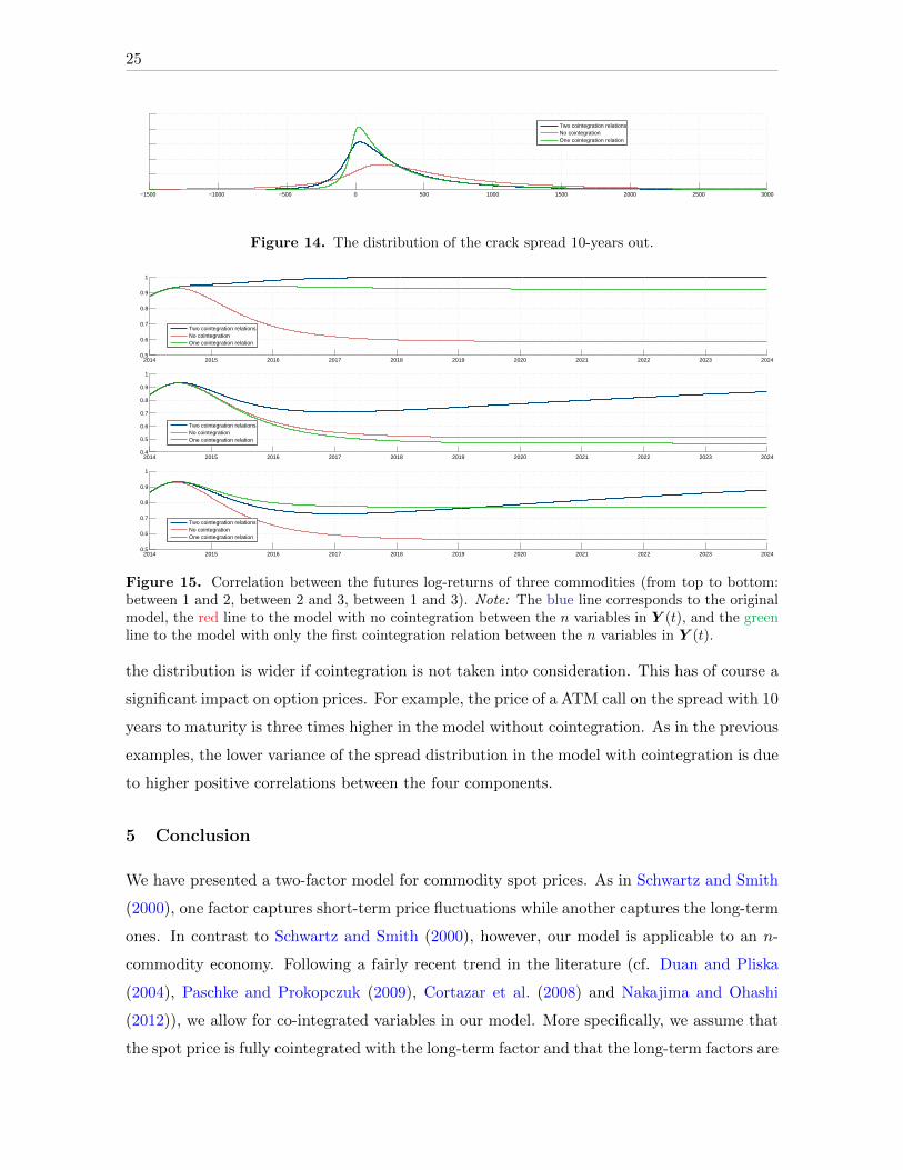
Figure 14. The distribution of the crack spread 10-years out.

2014 2015 2016 2017 2018 2019 2020 2021 2022 2023 20240.5

0.6

0.7

0.8

0.9

1


2014 2015 2016 2017 2018 2019 2020 2021 2022 2023 20240.4

0.5

0.6

0.7

0.8

0.9

1


2014 2015 2016 2017 2018 2019 2020 2021 2022 2023 20240.5

0.6

0.7

0.8

0.9

1


Figure 15. Correlation between the futures log-returns of three commodities (from top to bottom:between 1 and 2, between 2 and 3, between 1 and 3). Note: The blue line corresponds to the originalmodel, the red line to the model with no cointegration between the n variables in Y (t), and the greenline to the model with only the first cointegration relation between the n variables in Y (t).

the distribution is wider if cointegration is not taken into consideration. This has of course a

significant impact on option prices. For example, the price of a ATM call on the spread with 10

years to maturity is three times higher in the model without cointegration. As in the previous

examples, the lower variance of the spread distribution in the model with cointegration is due

to higher positive correlations between the four components.

5 Conclusion

We have presented a two-factor model for commodity spot prices. As in Schwartz and Smith

(2000), one factor captures short-term price fluctuations while another captures the long-term

ones. In contrast to Schwartz and Smith (2000), however, our model is applicable to an n-

commodity economy. Following a fairly recent trend in the literature (cf. Duan and Pliska

(2004), Paschke and Prokopczuk (2009), Cortazar et al. (2008) and Nakajima and Ohashi

(2012)), we allow for co-integrated variables in our model. More specifically, we assume that

the spot price is fully cointegrated with the long-term factor and that the long-term factors are

26

−300 −200 −100 0 100 200 300


Figure 16. The distribution of the power spread 10-years in the future.

cointegrated across commodities. As opposed to Paschke and Prokopczuk (2009) and Cortazar

et al. (2008), our model is capable of describing one up to n − 1 cointegration relationships

between the long-term factors of n commodities. The models of Duan and Pliska (2004) and

Nakajima and Ohashi (2012) could also be extended to include more than one cointegration

relationship but both models are defined in a convenience yield framework, which hinders a

transparent analysis (as also pointed out by Schwartz and Smith (2000)).

We have estimated our model using three alternative data sets. First, we used weekly

futures prices of crude oil, heating oil, gasoline and natural gas with a wide range of maturities,

spanning a period of over twenty years. We found two (statistically significant) cointegration

relationships. Only natural gas is not co-integrated with one of the others. Second, we again

used weekly futures prices, but now of electric power in four different regions. As expected, we

found that all of them are strongly cointegrated with each other. The third data set consisted

of futures prices on electric power and natural gas, and also here we found a cointegration

relationship.

Using the estimation results of our model, we have calculated the prices of several spread

options on energy commodities. The purpose here was merely to illustrate the effects of

cointegration. We found that cointegration affects the entire but particularly the long-end of

futures price term-structures. Furthermore, we found that cointegration leads to an upward

sloping correlation term-structure which lowers the volatility of spreads and therefore it also

lowers the value of options on spreads.

27

References

Alos, E., Eydeland, A., and Laurence, P. (2011). A Kirk and a Bachelier formula for three asset spread

options. Energy Risk, 9(2011):52–57.

Back, J. and Prokopczuk, M. (2013). Commodity price dynamics and derivative valuation: A review.

International Journal of Theoretical and Applied Finance, 16(6):1350032.

Back, J., Prokopczuk, M., and Rudolf, M. (2013). Seasonality and the valuation of commodity options.

Journal of Banking & Finance, 37:273n290.

Baillie, R. T. and Myers, R. J. (1991). Bivariate garch estimation of the optimal commodity futures

hedge. Journal of Applied Econometrics, 6(2):109–124.

Binder, K. (1987). Monte carlo methods. Quantum Monte Carlo Methods, page 241.

Bjerksund, P. and Stensland, G. (2011). Closed form spread option valuation. Quantitative Finance,

(ahead-of-print):1–10.

Black, F. (1976). Studies of stock price volatility changes. In Proceedings of the 1976 Meetings of the

American Statistical Association, pages 171–181.

Borovkova, S. and Geman, H. (2006). Seasonal and stochastic effects in commodity forward curves.

Review of Derivatives Research, 9:167 – 186.

Brenner, R. J. and Kroner, K. F. (1995). Arbitrage, cointegration, and testing the unbiasedness

hypothesis in financial markets. Journal of Financial and Quantitative Analysis, 30(01):23–42.

Caldana, R. and Fusai, G. (2013). A general closed-form spread option pricing formula. Journal of

Banking & Finance, 37:4893n4906.

Carbonell, F., Jimenez, J., and Pedroso, L. (2008). Computing multiple integrals involving matrix

exponentials. Journal of Computational and Applied Mathematics, 213(1):300–305.

Carmona, R. and Durrleman, V. (2003). Pricing and hedging spread options. Siam Review, 45(4):627–

685.

Comte, F. (1999). Discrete and continuous time cointegration. Journal of Econometrics, 88(2):207–226.

Cortazar, G., Milla, C., and Severino, F. (2008). A multicommodity model of futures prices: Using

futures prices of one commodity to estimate the stochastic process of another. Journal of Futures

Markets, 28(6):537–560.

Cortazar, G. and Naranjo, L. (2006). An N-factor gaussian model of oil futures prices. Journal of

Futures Markets, 26(3):243n268.

Crowder, W. J. and Hamed, A. (1993). A cointegration test for oil futures market efficiency. Journal

of Futures Markets, 13(8):933–941.

Dempster, M., Medova, E., and Tang, K. (2008). Long term spread option valuation and hedging.

Journal of Banking & Finance, 32(12):2530–2540.

Duan, J.-C. and Pliska, S. R. (2004). Option valuation with co-integrated asset prices. Journal of

Economic Dynamics and Control, 28(4):727–754.

28

Duffie, D. and Kan, R. (1996). A yield-factor model of interest rates. Mathematical Finance, 6:379–406.

Engle, R. F. and Granger, C. W. (1987). Co-integration and error correction: representation,

estimation, and testing. Econometrica, pages 251–276.

Geman, H. and Ohana, S. (2009). Forward curves, scarcity and price volatility in oil and natural gas

markets. Energy Economics, 31:576 – 585.

Gibson, R. and Schwartz, E. S. (1990). Stochastic convenience yield and the pricing of oil contingent

claims. The Journal of Finance, 45(3):959–976.

Hambly, B., Howison, S., and Kluge, T. (2009). Modelling spikes and pricing swing options in electricity

markets. Quantitative Finance, 9(8):937–949.

Johansen, S. (1991). Estimation and hypothesis testing of cointegration vectors in gaussian vector

autoregressive models. Econometrica, pages 1551–1580.

Kalman, R. E. (1960). A new approach to linear filtering and prediction problems. Journal of Fluids

Engineering, 82(1):35–45.

Kirk, E. (1995). Correlation in the energy markets. Managing energy price risk, pages 71–78.

Li, M., Zhou, J., and Deng, S.-J. (2010). Multi-asset spread option pricing and hedging. Quantitative

Finance, 10(3):305n324.

Lo, A. and Wang, J. (1995). Implementing option pricing models when asset returns are predictable.

Journal of Finance, 50:87n129.

Manoliu, M. and Tompaidis, S. (2002). Energy futures prices: term structure models with Kalman

filter estimation. Applied Mathematical Finance, 9:21 – 43.

Margrabe, W. (1978). The value of an option to exchange one asset for another. The Journal of

Finance, 33(1):177–186.

Nakajima, K. and Ohashi, K. (2012). A cointegrated commodity pricing model. Journal of Futures

Markets, 32(11):995–1033.

Paschke, R. and Prokopczuk, M. (2009). Integrating multiple commodities in a model of stochastic

price dynamics. Journal of Energy Markets, 2(3):47n82.

Paschke, R. and Prokopczuk, M. (2010). Commodity derivatives valuation with autoregressive and

moving average components in the price dynamics. Journal of Banking & Finance, 34:2742 –

2752.

Phillips, P. (1991). Error correction and long-run equilibrium in continuous time. Econometrica,

59(4):967–980.

Schwartz, E. and Smith, J. E. (2000). Short-term variations and long-term dynamics in commodity

prices. Management Science, 46(7):893–911.

Sorensen, C. (2002). Modeling seasonality in agricultural commodity futures. Journal of Futures

Markets, 22(5):393n426.

Welch, G. and Bishop, G. (1995). An introduction to the kalman filter.

29

A Lemmas

Lemma 1. The characteristic function of X(t+ τ) conditional on the information up to and

including time t, i.e.,

ϕX(t, τ, x, y;ω) := Et[exp

iω>X(t+ τ)

|X(t) = x,Y (t) = y

], (28)

is given by12

ϕX(t, τ, x, y;ω) = exp

iω>e−Kxτx+ iω>ψ(τ)y + iω>

[φ(t+ τ)− e−Kxτφ(t)

](29)

+ iω′[∫ τ

0ψ(τ − u)du

]µy

− 1

2

(ω>,0

)> [e−Kτ

(∫ τ

0eKuΣeK

>udu

)e−K

>τ

] (ω′,0

)>.

Proof. By straightforward calculations. q.e.d.

B Proof of Proposition 1

By the no-arbitrage assumption, the j-th futures price is given by

Fj(t, T ) = E∗t [Sj(T )] = E∗t [exp(Xj(T ))|X(t) = x,Y (t) = y] = ϕ∗X(t, τ, x, y;−iωj). (30)

where ϕ∗X(·) is the characteristic function of X(T ) under the risk-neutral measure, and where

ωj is a n-dimensional vector with the j-th component equal to 1 and the other components

equal to 0. Noting that ϕ∗X(·) is similar to ϕX(·) (see Lemma 1) but with µ replaced by µ∗,

we find

Fj(t, T ) = exp

ω>j e

−KxτX(t) + ω>j ψ(τ)Y (t) + ω>j[φ(t+ τ)− e−Kxτφ(t)

]+ ω>j

[∫ τ

0e−Kx(τ−u)du

]µ∗x + ω>j

[∫ τ

0ψ(τ − u)du

]µ∗y

+1

2

[ω>j 0>n

] [e−Kτ

(∫ τ

0eKuΣeKu

)e−K

>τ

]ω>j0n

.The proposition can be verified now by a straightforward calculation.

12The integrals appearing here can be computed explicitly using results in Carbonell et al. (2008).

30

C Estimation results

Below we report the parameter estimates 13 for data set I, II and III where λ := Σ12λ and

Σ :=

diag(σx) On

On diag(σy)

ρx ρxy

ρxy> ρy

diag(σx) On

On diag(σy)

.

Data set I:

µx =

0.00

0.00

0.00

0.00

, ˆλx =

0.10***

0.08***

0.13***

−0.10***

, Kx =

1.18*** 0.01 0.02** 0.01

0.04 1.18*** 0.01 −0.01

0.00 0.03 1.05*** 0.00

0.00 0.00 0.00 2.48***

,

σx =

0.35***

0.34***

0.34***

0.60***

, ρx =

1.00 0.88*** 0.86*** 0.26***

0.88*** 1.00 0.84*** 0.34***

0.86*** 0.84*** 1.00 0.26***

0.26*** 0.34*** 0.26*** 1.00

, µy =

2.27***

−1.88***

−0.29

−2.68**

, ˆλy =

0.13***

0.12***

0.15***

0.05

,

Ky =

0.64*** −0.11*** 0.00 0.00

−0.60*** 0.12 0.00 0.00

−0.10 −0.03 0.00 0.00

−0.76** 0.01 0.00 0.00

, Θ =

1.00 −0.69*** −0.28*** 0.03***

0.36*** 1.00 −1.47*** 0.05

0.00 0.00 0.00 0.00

0.00 0.00 0.00 0.00

,

σy =

0.23***

0.19***

0.28***

0.24***

, ρy =

1.00 0.59*** 0.56*** 0.08

0.59*** 1.00 0.51*** 0.28***

0.56*** 0.51*** 1.00 0.16**

0.08 0.28*** 0.16** 1.00

, ρxy =

0.48*** 0.64*** 0.50*** 0.22***

0.58*** 0.52*** 0.53*** 0.22***

0.53*** 0.62*** 0.29*** 0.22***

0.20*** 0.10** 0.14*** 0.37***

,

χ1 =

0.00

0.03***

−0.04***

−0.01***

, χ2 =

0.00

−0.01***

0.02***

0.01***

.13Statistical significance at 1% symbolized by ***, statistical significance at 5% symbolized by ** and statistical

significance at 10% symbolized by *.

31

Data set II:

µx =

0.00

0.00

0.00

0.00

, ˆλx =

−0.58***

−0.05

−0.08

0.07

, Kx =

1.59*** 0.39 0.20*** −0.02

−1.37** 2.55*** −0.24 0.35*

−4.51*** 1.27*** 4.95*** −0.26

−0.40 0.17 −0.13 1.38***

,

σx =

0.33***

0.51***

0.43***

0.23***

, ρx =

1.00 0.25*** 0.61*** 0.24***

0.25*** 1.00 0.25*** 0.27***

0.61*** 0.25*** 1.00 0.27***

0.24*** 0.27*** 0.27*** 1.00

, µy =

0.92***

0.87***

0.21

0.01

, ˆλy =

0.27*

0.30

0.22*

0.11

,

Ky =

0.78*** 1.20*** 0.25*** 0.00

−0.81*** 0.00 −0.05 0.00

0.24** 0.00 0.37*** 0.00

−0.17 −0.19*** 0.00 0.00

, Θ =

1.00 −1.33*** 0.00 0.00

0.00 1.00 −0.63*** 0.00

0.00 0.00 1.00 −0.74***

0.00 0.00 0.00 0.00

,

σy =

0.34***

0.42***

0.32***

0.29***

, ρy =

1.00 0.72*** 0.60*** 0.38***

0.72*** 1.00 0.42*** 0.48***

0.60*** 0.42*** 1.00 0.24***

0.38*** 0.48*** 0.24*** 1.00

, ρxy =

−0.01 −0.10 0.02 −0.14

0.39*** 0.37*** 0.45*** 0.17**

0.32*** 0.21 0.14*** 0.08

0.25** 0.15* 0.22* 0.28***

,

χ1 =

0.14***

0.13***

0.20***

−0.01***

, χ2 =

−0.01

0.01

0.01

0.02***

.

Data set III:

µx =

0.00

0.00

, ˆλx =

−0.59***

−0.36**

, Kx =

0.94** 0.60**

−4.15*** 2.41***

, σx =

0.30***

0.46***

, ρx =

1.00 0.31***

0.31*** 1.00

,µy =

−0.06

0.02

, ˆλy =

0.17*

0.52***

, Ky =

0.00 0.00

−0.02 0.00

, Θ =

1.00 −2.27***

0.00 0.00

, σy =

0.18***

0.30***

,ρy =

1.00 0.61***

0.61*** 1.00

, ρxy =

0.25** −0.33***

0.44*** 0.20

, χ1 =

0.12***

0.14***

, χ2 =

−0.09***

0.01

.

32

Figures 17 through 24 show values of the filtered X(t) and Y (t) and those of the estimated

seasonal component.

1991 1992 1993 1994 1995 1996 1997 1998 1999 2000 2001 2002 2003 2004 2005 2006 2007 2008 2009 2010 2011 2012 2013 20142

3

4

5

6

1991 1992 1993 1994 1995 1996 1997 1998 1999 2000 2001 2002 2003 2004 2005 2006 2007 2008 2009 2010 2011 2012 2013 2014−1

−0.5

0

0.5

1

1991 1992 1993 1994 1995 1996 1997 1998 1999 2000 2001 2002 2003 2004 2005 2006 2007 2008 2009 2010 2011 2012 2013 2014−1

−0.5

0

0.5

1x 10

−3

Figure 17. Top panel: Filtered time-series of spot log-prices X(t) (gray line) and long-run log-pricelevel Y (t) (red line) for crude oil. Middle panel: Differences between short- and long-term log-pricelevels, i.e., X(t)− φ(t)− Y (t). Bottom panel: Estimated seasonality function for crude oil.

1991 1992 1993 1994 1995 1996 1997 1998 1999 2000 2001 2002 2003 2004 2005 2006 2007 2008 2009 2010 2011 2012 2013 2014−1.5

−1

−0.5

0

0.5

1

1.5

1991 1992 1993 1994 1995 1996 1997 1998 1999 2000 2001 2002 2003 2004 2005 2006 2007 2008 2009 2010 2011 2012 2013 2014−1

−0.5

0

0.5

1

1991 1992 1993 1994 1995 1996 1997 1998 1999 2000 2001 2002 2003 2004 2005 2006 2007 2008 2009 2010 2011 2012 2013 2014−0.04

−0.02

0

0.02

0.04

Figure 18. Top panel: Filtered time-series of spot log-prices X(t) (gray line) and long-run log-price level Y (t) (red line) for heating oil. Middle panel: Differences between short- and long-termlog-price levels, i.e., X(t)− φ(t)−Y (t). Bottom panel: Estimated seasonality function for heatingoil.

33

1991 1992 1993 1994 1995 1996 1997 1998 1999 2000 2001 2002 2003 2004 2005 2006 2007 2008 2009 2010 2011 2012 2013 2014−1.5

−1

−0.5

0

0.5

1

1.5

1991 1992 1993 1994 1995 1996 1997 1998 1999 2000 2001 2002 2003 2004 2005 2006 2007 2008 2009 2010 2011 2012 2013 2014−1

−0.5

0

0.5

1

1991 1992 1993 1994 1995 1996 1997 1998 1999 2000 2001 2002 2003 2004 2005 2006 2007 2008 2009 2010 2011 2012 2013 2014−0.05

0

0.05

Figure 19. Top panel: Filtered time-series of spot log-prices X(t) (gray line) and long-run log-pricelevel Y (t) (red line) for gasoline. Middle panel: Differences between short- and long-term log-pricelevels, i.e., X(t)− φ(t)− Y (t). Bottom panel: Estimated seasonality function for gasoline.

1991 1992 1993 1994 1995 1996 1997 1998 1999 2000 2001 2002 2003 2004 2005 2006 2007 2008 2009 2010 2011 2012 2013 2014−1

0

1

2

3

1991 1992 1993 1994 1995 1996 1997 1998 1999 2000 2001 2002 2003 2004 2005 2006 2007 2008 2009 2010 2011 2012 2013 2014−1

−0.5

0

0.5

1

1991 1992 1993 1994 1995 1996 1997 1998 1999 2000 2001 2002 2003 2004 2005 2006 2007 2008 2009 2010 2011 2012 2013 2014−0.02

−0.01

0

0.01

0.02

Figure 20. Top panel: Filtered time-series of spot log-prices X(t) (gray line) and long-run log-pricelevel Y (t) (red line) for natural gas. Middle panel: Differences between short- and long-termlog-price levels, i.e., X(t)− φ(t)−Y (t). Bottom panel: Estimated seasonality function for naturalgas.

34

2007 2008 2009 2010 2011 2012 2013 20143

3.5

4

4.5

2007 2008 2009 2010 2011 2012 2013 2014−1

−0.5

0

0.5

2007 2008 2009 2010 2011 2012 2013 2014−0.2

−0.1

0

0.1

0.2

Figure 21. Top panel: Filtered time-series of spot log-prices X(t) (gray line) and long-run log-pricelevel Y (t) (red line) for power Germany. Middle panel: Differences between short- and long-termlog-price levels, i.e., X(t) − φ(t) − Y (t). Bottom panel: Estimated seasonality function for powerGermany.

2007 2008 2009 2010 2011 2012 2013 20142.5

3

3.5

4

4.5

2007 2008 2009 2010 2011 2012 2013 2014−1

−0.5

0

0.5

1

2007 2008 2009 2010 2011 2012 2013 2014−0.2

−0.1

0

0.1

0.2

Figure 22. Top panel: Filtered time-series of spot log-prices X(t) (gray line) and long-run log-pricelevel Y (t) (red line) for power Nordics. Middle panel: Differences between short- and long-termlog-price levels, i.e., X(t) − φ(t) − Y (t). Bottom panel: Estimated seasonality function for powerNordics.

35

2007 2008 2009 2010 2011 2012 2013 20143

3.5

4

4.5

2007 2008 2009 2010 2011 2012 2013 2014−1

−0.5

0

0.5

1

2007 2008 2009 2010 2011 2012 2013 2014−0.4

−0.2

0

0.2

0.4

Figure 23. Top panel: Filtered time-series of spot log-prices X(t) (gray line) and long-run log-pricelevel Y (t) (red line) for power Swiss. Middle panel: Differences between short- and long-termlog-price levels, i.e., X(t) − φ(t) − Y (t). Bottom panel: Estimated seasonality function for powerSwiss.

2007 2008 2009 2010 2011 2012 2013 20143

3.5

4

4.5

2007 2008 2009 2010 2011 2012 2013 2014−0.6

−0.4

−0.2

0

0.2

0.4

2007 2008 2009 2010 2011 2012 2013 2014−0.02

−0.01

0

0.01

0.02

Figure 24. Top panel: Filtered time-series of spot log-prices X(t) (gray line) and long-run log-pricelevel Y (t) (red line) for power Poland. Middle panel: Differences between short- and long-termlog-price levels, i.e., X(t) − φ(t) − Y (t). Bottom panel: Estimated seasonality function for powerPoland.

36

2006 2007 2008 2009 2010 2011 2012 2013 20143

3.5

4

4.5

2006 2007 2008 2009 2010 2011 2012 2013 2014−0.5

0

0.5

2006 2007 2008 2009 2010 2011 2012 2013 2014−0.2

−0.1

0

0.1

0.2

Figure 25. Top panel: Filtered time-series of spot log-prices X(t) (gray line) and long-run log-pricelevel Y (t) (red line) for electric power (data set III). Middle panel: Differences between short- andlong-term log-price levels, i.e., X(t) − φ(t) − Y (t). Bottom panel: Estimated seasonality functionfor electric power (data set III).

2006 2007 2008 2009 2010 2011 2012 2013 20141.5

2

2.5

3

3.5

2006 2007 2008 2009 2010 2011 2012 2013 2014−1.5

−1

−0.5

0

0.5

1

2006 2007 2008 2009 2010 2011 2012 2013 2014−0.2

−0.1

0

0.1

0.2

Figure 26. Top panel: Filtered time-series of spot log-prices X(t) (gray line) and long-run log-pricelevel Y (t) (red line) for natural gas (data set III). Middle panel: Differences between short- andlong-term log-price levels, i.e., X(t) − φ(t) − Y (t). Bottom panel: Estimated seasonality functionfor natural gas (data set III).

A Two-Factor Cointegrated Commodity Price Model with … ANNUAL MEETINGS/2015-… · A Two-Factor...

Documents

Transcript of A Two-Factor Cointegrated Commodity Price Model with … ANNUAL MEETINGS/2015-… · A Two-Factor...