Development of Simplified Analysis Procedure for Piles...

PACIFIC EARTHQUAKE ENGINEERING RESEARCH CENTER

Development of Simplified Analysis Procedure for Piles in Laterally Spreading Layered Soils

Christopher R. McGannPedro Arduino

Peter Mackenzie–HelnweinDepartment of Civil and Environmental Engineering

University of Washington

PEER 2012/05DECEMBER 2012

Disclaimer

The opinions, findings, and conclusions or recommendations expressed in this publication are those of the author(s) and do not necessarily reflect the views of the study sponsor(s) or the Pacific Earthquake Engineering Research Center.

Development of Simplified Analysis Procedure for Pilesin Laterally Spreading Layered Soils

Christopher R. McGannPedro Arduino

Peter Mackenzie-HelnweinDepartment of Civil and Environmental Engineering


PEER Report 2012/05Pacific Earthquake Engineering Research CenterHeadquarters, University of California, Berkeley

December 2012

ABSTRACT

This work presents the development of a simplified procedurefor the analysis of liquefaction–induced lateral spreading using a beam on nonlinear Winklerfoundation approach. A three-dimensional finite element model, considering a single pilein a soil continuum, is used to simulatelateral spreading and two alternative lateral load cases. Sets ofp –y curves representative of thesoil response in the 3D model are computed for various soil–pile systems. The affects of pile kine-matics on these curves are evaluated and a computational procedure forp –y curves is proposed.The computed curves are compared top –y curves defined by existing methods commonly used inpractice to evaluate the applicability of these methods to lateral spreading analysis.

Comparison of thep –y curves resulting from homogenous and layered soil profiles,in which aliquefied layer is located between two unliquefied layers, isused to identify reductions in the ulti-mate lateral resistance and initial stiffness of thep –y curves representing the unliquefied soil dueto the presence of the liquefied layer. These reductions are characterized in terms an exponentialdecay model. A simple procedure utilizing dimensionless parameters is proposed as a means ofimplementing appropriate reductions for an arbitrary soilprofile and pile diameter. Beam on non-linear Winkler foundation analyses of lateral spreading are conducted to validate and demonstratethe use of the proposed reduction procedure.

iii

ACKNOWLEDGMENTS

This work was supported by the State of California through the Transportation Systems ResearchProgram of the Pacific Earthquake Engineering Research (PEER) Center. Any opinions, findings,conclusions, or recommendations expressed in this material are those of the authors and do notnecessarily reflect those of the funding agency.

v

CONTENTS

ABSTRACT . . . . . . . . . . . . . . . . . . . . . . . . . . . . . . . . . . . . . . . . . iii

ACKNOWLEDGMENTS . . . . . . . . . . . . . . . . . . . . . . . . . . . . . . . . . v

TABLE OF CONTENTS . . . . . . . . . . . . . . . . . . . . . . . . . . . . . . . . . . vii

LIST OF FIGURES . . . . . . . . . . . . . . . . . . . . . . . . . . . . . . . . . . . . xiii

LIST OF TABLES . . . . . . . . . . . . . . . . . . . . . . . . . . . . . . . . . . . . . xix

1 INTRODUCTION . . . . . . . . . . . . . . . . . . . . . . . . . . . . . . . . . . . 1

1.1 Background . . . . . . . . . . . . . . . . . . . . . . . . . . . . . . . . . . . . . .2

1.2 Scope of Work . . . . . . . . . . . . . . . . . . . . . . . . . . . . . . . . . . . . 4

2 THREE-DIMENSIONAL FINITE ELEMENT MODEL . . . . . . . . . . . . . . 7

2.1 Introduction . . . . . . . . . . . . . . . . . . . . . . . . . . . . . . . . . . . .. . 7

2.2 Model Overview . . . . . . . . . . . . . . . . . . . . . . . . . . . . . . . . . . .7

2.2.1 Selective Mesh Refinement . . . . . . . . . . . . . . . . . . . . . . . .. . 8

2.3 Boundary and Loading Conditions . . . . . . . . . . . . . . . . . . . .. . . . . . 9

2.3.1 Loading Conditions . . . . . . . . . . . . . . . . . . . . . . . . . . . . .. 9

2.4 Modeling the Soil-Pile Interface . . . . . . . . . . . . . . . . . . .. . . . . . . . 10

2.4.1 Beam-Solid Contact Elements . . . . . . . . . . . . . . . . . . . . .. . . 10

2.5 Surface Load Elements . . . . . . . . . . . . . . . . . . . . . . . . . . . . .. . . 11

2.5.1 Formulation of Surface Load Elements . . . . . . . . . . . . . .. . . . . 12

2.5.2 Validation of Surface Elements . . . . . . . . . . . . . . . . . . .. . . . . 14

3 MODELING THE PILES . . . . . . . . . . . . . . . . . . . . . . . . . . . . . . . 17

3.1 Introduction . . . . . . . . . . . . . . . . . . . . . . . . . . . . . . . . . . . .. . 17

3.2 Template Pile Designs . . . . . . . . . . . . . . . . . . . . . . . . . . . . .. . . 17

3.3 Pile Elements . . . . . . . . . . . . . . . . . . . . . . . . . . . . . . . . . . . .. 18

3.3.1 Fiber Section Models . . . . . . . . . . . . . . . . . . . . . . . . . . . .. 19

3.4 Linear Elastic Pile Constitutive Behavior . . . . . . . . . . .. . . . . . . . . . . . 20

3.5 Elastoplastic Pile Constitutive Behavior . . . . . . . . . . .. . . . . . . . . . . . 20

3.5.1 Steel in Tension and Compression . . . . . . . . . . . . . . . . . .. . . . 22

vii

3.5.2 Concrete in Compression . . . . . . . . . . . . . . . . . . . . . . . . .. . 22

3.5.3 Concrete in Tension . . . . . . . . . . . . . . . . . . . . . . . . . . . . .23

3.5.4 One-Dimensional Fracture Mechanics of Concrete in Tension . . . . . . . 24

3.5.5 Implementation of Tension Parameters . . . . . . . . . . . . .. . . . . . . 26

3.6 Validation of Pile Models . . . . . . . . . . . . . . . . . . . . . . . . . .. . . . . 30

3.6.1 Moment-Curvature Response . . . . . . . . . . . . . . . . . . . . . .. . 30

3.6.2 Validation of Tension Parameters . . . . . . . . . . . . . . . . .. . . . . 36

4 MODELING THE SOIL . . . . . . . . . . . . . . . . . . . . . . . . . . . . . . . . 41

4.1 Introduction . . . . . . . . . . . . . . . . . . . . . . . . . . . . . . . . . . . .. . 41

4.2 Soil Elements . . . . . . . . . . . . . . . . . . . . . . . . . . . . . . . . . . . .. 41

4.3 Linear Elastic Soil Constitutive Modeling . . . . . . . . . . .. . . . . . . . . . . 42

4.4 Elastoplastic Soil Constitutive Modeling . . . . . . . . . . .. . . . . . . . . . . . 42

4.4.1 Drucker-Prager Constitutive Model . . . . . . . . . . . . . . .. . . . . . 43

4.4.2 Determination of Material Parameters . . . . . . . . . . . . .. . . . . . . 46

4.5 Validation of Soil Models . . . . . . . . . . . . . . . . . . . . . . . . . .. . . . . 47

4.5.1 Confined Compression Test . . . . . . . . . . . . . . . . . . . . . . . .. 48

4.5.2 Conventional Triaxial Compression Test . . . . . . . . . . .. . . . . . . . 50

4.5.3 Simple Shear Test . . . . . . . . . . . . . . . . . . . . . . . . . . . . . . 54

4.5.4 Hydrostatic Extension Test . . . . . . . . . . . . . . . . . . . . . .. . . . 57

4.5.5 Multi-Element Plane Strain Test . . . . . . . . . . . . . . . . . .. . . . . 59

5 THREE-DIMENSIONAL FINITE ELEMENT ANALYSIS . . . . . . . . . . . . . 61

5.1 Introduction . . . . . . . . . . . . . . . . . . . . . . . . . . . . . . . . . . . .. . 61

5.2 Summary of Considered Cases . . . . . . . . . . . . . . . . . . . . . . . .. . . . 62

5.2.1 Series 1: Elastic Piles with Elastic Soil . . . . . . . . . . .. . . . . . . . 62

5.2.2 Series 2: Elastoplastic Piles with Elastic Soil . . . . .. . . . . . . . . . . 63

5.2.3 Series 3: Elastic Piles with Elastoplastic Soil . . . . .. . . . . . . . . . . 63

5.2.4 Series 4: Elastoplastic Piles in Elastoplastic Soil .. . . . . . . . . . . . . 63

5.3 General Behavior of Piles in Laterally Spreading Soil . .. . . . . . . . . . . . . . 64

5.4 Summary of Results from Three-Dimensional Lateral Spreading Simulations . . . 68

5.4.1 The Effects of Pile Stiffness on the Soil-Pile System .. . . . . . . . . . . 70

viii

5.4.2 The Effects of Pile Head Fixity . . . . . . . . . . . . . . . . . . . .. . . 72

5.5 The Effects of Plasticity on the Laterally Spreading System . . . . . . . . . . . . . 75

5.5.1 The Effects of Pile Plasticity . . . . . . . . . . . . . . . . . . . .. . . . . 75

5.5.2 The Effects of Soil Plasticity on the Pile . . . . . . . . . . .. . . . . . . . 75

5.6 Verification Models for Pile Behavior in Elastoplastic Soil . . . . . . . . . . . . . 76

5.6.1 The First Simple Model . . . . . . . . . . . . . . . . . . . . . . . . . . .78

5.6.2 The Second Simple Model . . . . . . . . . . . . . . . . . . . . . . . . . .81

5.6.3 Observations . . . . . . . . . . . . . . . . . . . . . . . . . . . . . . . . . 83

5.7 Summary . . . . . . . . . . . . . . . . . . . . . . . . . . . . . . . . . . . . . . . 85

6 COMPUTATION OF REPRESENTATIVE p –y CURVES FROM THE THREE-DIMENSIONAL MODEL . . . . . . . . . . . . . . . . . . . . . . . . . . . . . . . 87

6.1 Introduction . . . . . . . . . . . . . . . . . . . . . . . . . . . . . . . . . . . .. . 87

6.2 Computation of Force and Displacement Histories . . . . . .. . . . . . . . . . . . 87

6.3 Considered Kinematic Cases . . . . . . . . . . . . . . . . . . . . . . . .. . . . . 89

6.4 Curve-fitting Strategies . . . . . . . . . . . . . . . . . . . . . . . . . .. . . . . . 89

6.4.1 Hyperbolic Tangent Function . . . . . . . . . . . . . . . . . . . . .. . . 90

6.4.2 Polynomial Function . . . . . . . . . . . . . . . . . . . . . . . . . . . .. 91

6.5 Effects of Pile Kinematics on Computedp –y Curves . . . . . . . . . . . . . . . . 93

6.5.1 Betti-Rayleigh Theorem of Reciprocal Work . . . . . . . . .. . . . . . . 98

6.5.2 Application of the Betti-Rayleigh Theorem . . . . . . . . .. . . . . . . . 98

6.5.3 Proposed Solution to the Problem of Pile Kinematics . .. . . . . . . . . . 99

6.6 Effects of Selective Mesh Refinement on Computedp –y Curves . . . . . . . . . . 100

6.7 Boundary Effects on Soil Response . . . . . . . . . . . . . . . . . . .. . . . . . . 102

6.8 Summary . . . . . . . . . . . . . . . . . . . . . . . . . . . . . . . . . . . . . . . 107

7 APPLICABILITY OF CONVENTIONAL AND COMPUTED p –y CURVES TOLATERAL SPREADING ANALYSIS . . . . . . . . . . . . . . . . . . . . . . . . . 109

7.1 Introduction . . . . . . . . . . . . . . . . . . . . . . . . . . . . . . . . . . . .. . 109

7.2 A Brief Summary of the Considered Predictive Methods . . .. . . . . . . . . . . 109

7.2.1 Ultimate Lateral Resistance . . . . . . . . . . . . . . . . . . . . .. . . . 110

7.2.2 Initial Stiffness . . . . . . . . . . . . . . . . . . . . . . . . . . . . . .. . 113

7.3 Comparison of Computed and Predictedp –y Curves . . . . . . . . . . . . . . . . 115

ix

7.3.1 Comparison of Ultimate Lateral Resistance . . . . . . . . .. . . . . . . . 115

7.3.2 Comparison of Initial Stiffness . . . . . . . . . . . . . . . . . .. . . . . . 118

7.3.3 Comparison ofp –y Curves . . . . . . . . . . . . . . . . . . . . . . . . . 121

7.4 Near-Surface Models . . . . . . . . . . . . . . . . . . . . . . . . . . . . . .. . . 121

7.4.1 Initial Stiffness Distributions in Near-Surface Models . . . . . . . . . . . . 124

7.4.2 Ultimate Lateral Resistance Distributions in Near-Surface Models . . . . . 124

7.5 Plane Strain Models . . . . . . . . . . . . . . . . . . . . . . . . . . . . . . .. . . 125

7.6 Summary . . . . . . . . . . . . . . . . . . . . . . . . . . . . . . . . . . . . . . . 127

8 INFLUENCE OF LIQUEFIED LAYER ON THE SOIL RESPONSE . . . . . . . . 129

8.1 Introduction . . . . . . . . . . . . . . . . . . . . . . . . . . . . . . . . . . . .. . 129

8.2 Initial Observations . . . . . . . . . . . . . . . . . . . . . . . . . . . . .. . . . . 129

8.3 Updated Finite Element Model . . . . . . . . . . . . . . . . . . . . . . .. . . . . 134

8.3.1 Considered Soil Profiles . . . . . . . . . . . . . . . . . . . . . . . . .. . 134

8.4 Characterizing the Influence of the Liquefied Layer . . . . .. . . . . . . . . . . . 135

8.4.1 Reduction in Ultimate Lateral Resistance . . . . . . . . . .. . . . . . . . 135

8.4.2 Reduction in Initial Stiffness . . . . . . . . . . . . . . . . . . .. . . . . . 135

8.5 Reduction Model . . . . . . . . . . . . . . . . . . . . . . . . . . . . . . . . . .. 139

8.5.1 Parameter Identification . . . . . . . . . . . . . . . . . . . . . . . .. . . 139

8.6 Reduction Procedure . . . . . . . . . . . . . . . . . . . . . . . . . . . . . .. . . 140

8.7 Summary . . . . . . . . . . . . . . . . . . . . . . . . . . . . . . . . . . . . . . . 142

9 BEAM ON NONLINEAR WINKLER FOUNDATION ANALYSIS . . . . . . . . . 145

9.1 Introduction . . . . . . . . . . . . . . . . . . . . . . . . . . . . . . . . . . . .. . 145

9.2 Evaluation of Computed and Predictedp –y Curves . . . . . . . . . . . . . . . . . 146

9.2.1 Beam on Nonlinear Winkler Foundation Model . . . . . . . . .. . . . . . 146

9.2.2 Modeling thep –y Curves . . . . . . . . . . . . . . . . . . . . . . . . . . 147

9.2.3 Consideredp –y Curves . . . . . . . . . . . . . . . . . . . . . . . . . . . 147

9.2.4 Results . . . . . . . . . . . . . . . . . . . . . . . . . . . . . . . . . . . . 148

9.3 Validation and Application of Proposed Curve ReductionProcedure . . . . . . . . 153

9.3.1 Test Profiles . . . . . . . . . . . . . . . . . . . . . . . . . . . . . . . . . . 153

9.3.2 Investigated Test Cases . . . . . . . . . . . . . . . . . . . . . . . . .. . . 154

x

9.3.3 Results . . . . . . . . . . . . . . . . . . . . . . . . . . . . . . . . . . . . 156

9.4 Effects of Soil Shear Modulus on Initial Stiffness ofp –y Curves . . . . . . . . . . 158

9.5 Summary . . . . . . . . . . . . . . . . . . . . . . . . . . . . . . . . . . . . . . . 160

10 SUMMARY, CONCLUSIONS, AND RECOMMENDATIONS FOR FUTURE WO RK 163

10.1 Summary and Conclusions . . . . . . . . . . . . . . . . . . . . . . . . . .. . . . 163

10.2 Recommendations for Future Work . . . . . . . . . . . . . . . . . . .. . . . . . . 168

REFERENCES . . . . . . . . . . . . . . . . . . . . . . . . . . . . . . . . . . . . . . . 171

xi

LIST OF FIGURES

1.1 Schematic depicting the layered lateral spreading soil-pile system. . . . . . . . . . 2

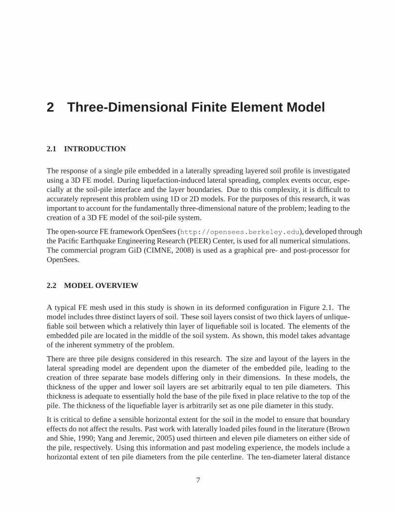
2.1 Typical finite element mesh for soil-pile system in deformed configuration. . . . . 8

2.2 A depiction of the imposed displacement profile for the lateral spreading model. . . 10

2.3 A top view of the finite element mesh for the soil mass. The pile is the dot in thecenter of the lower edge. . . . . . . . . . . . . . . . . . . . . . . . . . . . . . .. 11

2.4 Details of the deformation in the soil elements around the pile using beam-solidcontact elements. . . . . . . . . . . . . . . . . . . . . . . . . . . . . . . . . . . .11

2.5 Irregularly-shaped mesh used for surface load element validation. . . . . . . . . . 14

2.6 Distribution of vertical stress in the surface load element validation model. . . . . . 15

3.1 Template pile designs (to scale). (a) 0.61-m-diameter;(b) 1.37-m-diameter; (c)2.5-m-diameter. . . . . . . . . . . . . . . . . . . . . . . . . . . . . . . . . . . . .17

3.2 Dimensions and details of the three template piles. (a) 0.61-m-diameter; (b) 1.37-m-diameter; (c) 2.5-m-diameter. . . . . . . . . . . . . . . . . . . . . . .. . . . . 18

3.3 Typical fiber discretization for a circular fiber sectionmodel. . . . . . . . . . . . . 19

3.4 Uniaxial constitutive relations used in fiber section models. (a)Concrete02model.(b) Steel01model. . . . . . . . . . . . . . . . . . . . . . . . . . . . . . . . . . . . 21

3.5 Detail of tensile behavior in uniaxial concrete constitutive model. . . . . . . . . . . 23

3.6 Simplified fracture model for concrete in uniaxial tension. . . . . . . . . . . . . . 24

3.7 Relationship between elongation, crack width, and element length for a single pileelement. . . . . . . . . . . . . . . . . . . . . . . . . . . . . . . . . . . . . . . . . 25

3.8 Moment-curvature behavior for 0.61-m-diameter model illustrating softening be-havior resulting from a large characteristic length,ℓc. . . . . . . . . . . . . . . . . 28

3.9 Moment-curvature behavior for 2.5-m-diameter model with two values of charac-teristic length,ℓc. . . . . . . . . . . . . . . . . . . . . . . . . . . . . . . . . . . . 28

3.10 Moment-curvature behavior for 0.61-m-diameter modelwith various values ofℓc.Largest element length is0.649 m. Smallest element length is0.102 m. . . . . . . . 29

3.11 Moment-curvature behavior for 1.37-m-diameter modelwith various values ofℓc.Largest element length is1.79 m. Smallest element length is0.231 m. . . . . . . . 29

3.12 Distributions of stress and strain determined for 0.61-m-diameter cross section. . . 32

xiii

3.13 Comparison of moment-curvature responses for 0.61-m-diameter full (circular)pile model. . . . . . . . . . . . . . . . . . . . . . . . . . . . . . . . . . . . . . . 33

3.14 Comparison of moment-curvature responses for 0.61-m-diameter half-pile (semi-circular) model. . . . . . . . . . . . . . . . . . . . . . . . . . . . . . . . . . . . .33

3.15 Comparison of moment-curvature responses for 1.37-m-diameter full (circular)pile model. . . . . . . . . . . . . . . . . . . . . . . . . . . . . . . . . . . . . . . 34


3.17 Comparison of moment-curvature responses for 2.5-m-diameter full (circular) pilemodel. . . . . . . . . . . . . . . . . . . . . . . . . . . . . . . . . . . . . . . . . . 35


3.19 Cantilever beam analysis. The horizontal load, P, is increased linearly until the piletip deflects a distance of one pile radius. . . . . . . . . . . . . . . . .. . . . . . . 36

3.20 Moment-curvature response of cantilever model compared to zero-length elementand independently calculated section responses for 0.61-m-diameter section. Thecantilever model fails at this level of curvature. . . . . . . . .. . . . . . . . . . . 37

3.21 Moment-curvature response of cantilever model compared to zero-length elementand independently calculated section responses for 2.5-m-diameter section. . . . . 37

3.22 Force-displacement behavior for 0.61-m-pile sectionmodel as implemented in acantilever beam model with various values ofℓc. . . . . . . . . . . . . . . . . . . . 38

3.23 Force-displacement behavior for 1.37-m-pile sectionmodel as implemented in acantilever beam model with various values ofℓc. . . . . . . . . . . . . . . . . . . . 39

4.1 Drucker-Prager failure surface plotted in principal stress space. . . . . . . . . . . . 43

4.2 Schematic depiction of the simulated CC test. (a) Hydrostatic compression phase;(b) Confined compression phase. . . . . . . . . . . . . . . . . . . . . . . . .. . . 48

4.3 Stress paths for CC test. . . . . . . . . . . . . . . . . . . . . . . . . . . .. . . . . 49

4.4 Stress-strain responses of Drucker-Prager soil element subjected to CC test stresspath. . . . . . . . . . . . . . . . . . . . . . . . . . . . . . . . . . . . . . . . . . . 49

4.5 Schematic depiction of the CTC test as performed in OpenSees. (a) Hydrostaticcompression phase; (b) Application of deviator stress. . . .. . . . . . . . . . . . . 50

4.6 Comparison of simulated and theoretical CTC test stresspaths. . . . . . . . . . . . 51

4.7 Stress paths for CTC test in the perfectly plastic case (no strain hardening). . . . . 52

4.8 Stress paths for CTC test the linear isotropic strain hardening case. . . . . . . . . . 52

xiv

4.9 Stress-strain responses of Drucker-Prager soil element subjected to a CTC stresspath for the perfectly plastic case (no strain hardening). .. . . . . . . . . . . . . . 53

4.10 Stress-strain responses of Drucker-Prager soil element subjected to a CTC stresspath for the linear isotropic strain hardening case. . . . . . .. . . . . . . . . . . . 53

4.11 Schematic depiction of the SS test as performed in OpenSees. (a) Hydrostaticcompression phase; (b) Simple shear phase. . . . . . . . . . . . . . .. . . . . . . 54

4.12 Stress paths for SS test in the perfectly plastic case (no strain hardening). . . . . . . 55

4.13 Stress-strain responses of Drucker-Prager soil element subjected to a SS test stresspath for the perfectly plastic case (no strain hardening). .. . . . . . . . . . . . . . 55

4.14 Stress paths for SS test in the linear isotropic strain hardening case. . . . . . . . . . 56

4.15 Stress-strain responses of Drucker-Prager soil element subjected to a SS test stresspath for the linear isotropic strain hardening case. . . . . . .. . . . . . . . . . . . 56

4.16 Schematic depiction of the HE test as performed in OpenSees. . . . . . . . . . . . 57

4.17 Stress paths for HE test, on the meridian plane for threevalues of the tensionsoftening parameter,δ. . . . . . . . . . . . . . . . . . . . . . . . . . . . . . . . . 58

4.18 Stress-strain response of Drucker-Prager soil element subjected to a HE test stresspath for three values of tension softening parameter,δ. . . . . . . . . . . . . . . . 58

4.19 A representation of the load case modeled by the multi-element plane strain testfor the Drucker-Prager material model. . . . . . . . . . . . . . . . . .. . . . . . . 59

4.20 The deformed mesh for the plane strain test with the distribution of vertical stressin the soil elements (magnification factor = 10). . . . . . . . . . .. . . . . . . . . 60

4.21 Stress paths for a selection of Gauss points along the top row of the plane strainmodel. . . . . . . . . . . . . . . . . . . . . . . . . . . . . . . . . . . . . . . . . . 60

5.1 Deformed shape and distribution of lateral stress for the Series1 free-head casewith a 0.61-m-diameter pile. Stresses are given in kPa. . . . .. . . . . . . . . . . 64

5.2 Pile summary plots for a 0.61-m-diameter pile. Series 1,free-head case. Theliquefied layer is the shaded region. . . . . . . . . . . . . . . . . . . . .. . . . . 66

5.3 The effective length,Leff , is the distance between the extreme moments in eachsolid soil layer, as shown in this moment diagram. . . . . . . . . .. . . . . . . . . 67

5.4 Soil deformation pattern in the vicinity the pile for theSeries4 case highlightingthe unliquefied soil elements pushing into the liquefied layer. . . . . . . . . . . . . 68

5.5 Load distributions resulting from the lateral spreading ground motion for the free-head Series 1 cases for 0.61-m and 2.5-m-diameter piles. . . .. . . . . . . . . . . 70

5.6 Deflected shapes of free-head piles for various cases. (a) Series 1, 0.61-m-diameter;(b) Series 1, 2.5-m-diameter; (c) Series 2, 0.61-m-diameter; (d) Series 2, 2.5-m-diameter. . . . . . . . . . . . . . . . . . . . . . . . . . . . . . . . . . . . . . . . . 71

xv

5.7 Upward heave of soil elements at the ground surface for the Series 4 case with a2.5-m-diameter pile (magnification factor = 1). . . . . . . . . . .. . . . . . . . . 73

5.8 Moment distributions and deflected shapes for the fixed-head Series 1 cases with2.5-m and 1.37-m-diameter piles. . . . . . . . . . . . . . . . . . . . . . .. . . . . 74

5.9 Pile summary plots for a 0.61-m-diameter pile. Series 3,free-head case. Theliquefied layer is the shaded region. . . . . . . . . . . . . . . . . . . . .. . . . . 77

5.10 The two simple beam models used for verification of results. (a) The first simplemodel. (b) The second simple model. . . . . . . . . . . . . . . . . . . . . .. . . 78

5.11 Displaced shape, shear diagram, and moment diagram forthe first simple model. . 80

5.12 Displaced shape, shear diagram, and moment diagram forthe second simple model. 83

5.13 Normalized relationships betweenLeff , maxM , andp for the two simple models. . 84

6.1 Computation ofp –y curves from the 3D FE model. . . . . . . . . . . . . . . . . . 88

6.2 Determination of displacements suitable for use inp - y curves for the lateral spread-ing case. . . . . . . . . . . . . . . . . . . . . . . . . . . . . . . . . . . . . . . . . 88

6.3 Pile kinematic cases. (a) Lateral Spreading; (b) Top pushover; (c) Rigid pile. . . . . 89

6.4 Example of computedp –y data with fitted initial tangent stiffness and hyperbolictangent curve for a 1.37 m diameter pile. . . . . . . . . . . . . . . . . .. . . . . . 92

6.5 The lateral resistance ratio, LRR, is the ratio of the soil resistance values computedin two referencep –y curves at a prescribed value of displacement. . . . . . . . . . 93

6.6 Comparison of the lateral spreading kinematic case to the rigid pile case for a 1.37-m-diameter pile. Both analyses use a three-layer liquefied soil system. . . . . . . . 95

6.7 Comparison of the top pushover kinematic case to the rigid pile case for a a 1.37-m-diameter pile. Both analyses use homogenous soil profiles. . . . . . . . . . . . . 95

6.8 Computedp –y curves from the top pushover and rigid pile cases in homogenoussoil for a 0.61-m-diameter pile. The fitted initial tangentsare shown for each case. . 96

6.9 Computedp –y curves from the lateral spreading and rigid pile cases in non-homogenous soil for a 0.61-m-diameter pile. The fitted initial tangents are shownfor each case. . . . . . . . . . . . . . . . . . . . . . . . . . . . . . . . . . . . . . 97

6.10 Two separate load cases,P andQ, with respective displacements,u andv, appliedto the same points on a general elastic body. . . . . . . . . . . . . . .. . . . . . . 98

6.11 Distributions ofkT andpu for 1.37-m-diameter pile in homogenous soil profile. . . 101

6.12 Examples of smoothing process on curve parameters for 1.37-m-diameter pile. (a)Distribution of pu from rigid pile in liquefied soil profile; b) Distribution ofkTfrom rigid pile in liquefied soil profile; (c) Distribution ofkT from top pushover inhomogenous soil profile. . . . . . . . . . . . . . . . . . . . . . . . . . . . . . .. 101

xvi

6.13 Laterally-extended mesh for 0.61-m-pile design. . . . .. . . . . . . . . . . . . . . 103

6.14 Comparison ofp –y curve parameter distributions for extended and standard meshesfor a 0.61-m-diameter pile. . . . . . . . . . . . . . . . . . . . . . . . . . . .. . . 104

6.15 Plan view showing the distribution of vertical displacement (i.e., soil heave) in thesoil elements. The areas near the pile indicate the greatestmagnitude of displace-ment, while the constantly shaded areas near the boundarieshave zero displacement.104

6.16 Contour plot of vertical soil displacements in the extended mesh. Only upwarddisplacements are considered. . . . . . . . . . . . . . . . . . . . . . . . .. . . . 105

6.17 Contour plot of vertical soil displacements for the rigid pile case in the standardmesh. Only upward displacements are considered. . . . . . . . . .. . . . . . . . . 105

6.18 Distribution of the first invariant of stress,I1, in the standard mesh for a 0.61-m-diameter pile. . . . . . . . . . . . . . . . . . . . . . . . . . . . . . . . . . . . . . 106

6.19 Distribution of the first invariant of stress,I1, in the extended mesh for a 0.61-m-diameter pile. . . . . . . . . . . . . . . . . . . . . . . . . . . . . . . . . . . . . . 106

7.1 Distributions of ultimate lateral resistance for a 0.5-m-diameter pile as specifiedby four predictive methods. . . . . . . . . . . . . . . . . . . . . . . . . . . .. . . 110

7.2 Recommended coefficient of subgrade reaction after API (1987). The conversionfrom units of lb/in3 is obtained through multiplication with a factor of 271.45 toobtain units of kN/m3. . . . . . . . . . . . . . . . . . . . . . . . . . . . . . . . . 114

7.3 Distributions of ultimate lateral resistance and initial stiffness for each of the threetemplate pile designs as compared to commonly referenced distributions. . . . . . 116

7.4 Comparison of computedp –y data with fitted hyperbolic tangent curves for a 2.5-m-diameter pile. . . . . . . . . . . . . . . . . . . . . . . . . . . . . . . . . . . . .117

7.5 Distribution of stress in the direction of loading at full lateral displacement of a0.61-m-diameter pile in the rigid pile kinematic case. . . . .. . . . . . . . . . . . 118

7.6 Norm of the deviatoric plastic strain,||ep||, for a 0.61-m-diameter pile. . . . . . . . 119

7.7 Linear elastic and elastoplastickT distributions computed from 3D FE analysis. . . 120

7.8 Computed and API recommendedp –y curves for a 1.37-m-diameter pile. . . . . . 121

7.9 Near-surface mesh for a 1.37-m-diameter pile. . . . . . . . .. . . . . . . . . . . . 122

7.10 Comparisonpu andkT distributions for default and near-surface meshes over thefirst 10 m below the ground surface. . . . . . . . . . . . . . . . . . . . . . .. . . 123

7.11 Distributions of initial stiffness computed from the near-surface models using bothelastoplastic and elastic soil elements. . . . . . . . . . . . . . . .. . . . . . . . . 124

7.12 Computedpu distributions for near-surface models. . . . . . . . . . . . . . . . .. 125

7.13 Comparison parameter distributions for default and plane strain FE models. . . . . 126

xvii

7.14 Comparison of estimatedpu distributions with corresponding results from planestrain model for a 2.5-m-diameter pile. . . . . . . . . . . . . . . . . .. . . . . . . 127

8.1 Distributions ofpu andkT for homogenous and liquefied soil profiles for a 1.37-m-diameter pile. . . . . . . . . . . . . . . . . . . . . . . . . . . . . . . . . . . . .130

8.2 Computedpu ratios for a series of overburden pressures,pvo. The five cases arecompared at lower right. . . . . . . . . . . . . . . . . . . . . . . . . . . . . . .. 132

8.3 ComputedkT ratios for a series of overburden pressures,pvo. The five cases arecompared at lower right. . . . . . . . . . . . . . . . . . . . . . . . . . . . . . .. 133

8.4 Updated layered soil 3D FE mesh. . . . . . . . . . . . . . . . . . . . . .. . . . . 134

8.5 Comparison ofpu andkT in homogenous and liquefied soil profiles for a 0.61-m-diameter pile. . . . . . . . . . . . . . . . . . . . . . . . . . . . . . . . . . . . . . 136

8.6 Computedpu ratios above the liquefied layer for a 0.61-m-diameter pile.. . . . . . 137

8.7 Computedpu ratios below the liquefied layer for a 0.61-m-diameter pile.. . . . . . 137

8.8 ComputedkT ratios above the liquefied layer for a 1.37-m-diameter pile.. . . . . . 138

8.9 ComputedkT ratios below the liquefied layer for a 1.37-m-diameter pile.. . . . . . 138

8.10 Dimensionless relations forpu above and below the liquefied layer. . . . . . . . . . 140

8.11 Dimensionless relations forkT above and below the liquefied layer. . . . . . . . . . 141

9.1 Schematic representation of the BNWF model. . . . . . . . . . .. . . . . . . . . 146

9.2 Deflected shape, shear force, and moment diagrams for BNWF and 3D FE analysesof lateral spreading for a 1.37-m-diameter pile with linearelastic behavior. . . . . . 152

9.3 Evolution of extreme moment demands in top and bottom layers with increasingdisplacement of upper soil layer during BNWF and 3D FE lateral spreading anal-yses for a 1.37-m-diameter pile. . . . . . . . . . . . . . . . . . . . . . . .. . . . 153

9.4 Distributions ofpu used in BNWF models. . . . . . . . . . . . . . . . . . . . . . . 155

9.5 Distributions ofkT used in BNWF models. . . . . . . . . . . . . . . . . . . . . . 155

9.6 Comparison of maximum pile shear and moment demands. . . .. . . . . . . . . . 156

9.7 Deformed shapes of pile in theVC2andPC3BNWF analyses. . . . . . . . . . . . 158

9.8 Comparison of initial stiffness distributions for various values of soil shear modu-lus,G. . . . . . . . . . . . . . . . . . . . . . . . . . . . . . . . . . . . . . . . . . 159

9.9 Comparison of maximum pile shear and moment demands for higher shear modu-lus cases. . . . . . . . . . . . . . . . . . . . . . . . . . . . . . . . . . . . . . . . 160

xviii

LIST OF TABLES

3.1 Material and section property values in linear elastic pile models. . . . . . . . . . . 20

3.2 Steel material property input values in fiber section models. . . . . . . . . . . . . . 21

3.3 Concrete material property input values in fiber sectionmodels. . . . . . . . . . . . 21

3.4 Concrete fracture energies and crack propagation slopes. . . . . . . . . . . . . . . 25

3.5 Characteristic length and tension softening modulus inpile models. . . . . . . . . 27

4.1 Material parameters in isotropic linear elastic soil constitutive model. . . . . . . . 42

4.2 Material input parameters used in Drucker-Prager soil constitutive model. . . . . . 47

5.1 Overview of the four considered test Series. . . . . . . . . . .. . . . . . . . . . . 62

5.2 Summary of 3D lateral spreading analyses for the 2.5-m-diameter pile. . . . . . . . 69

5.3 Summary of 3D lateral spreading analyses for the 1.37-m-diameter pile. . . . . . . 69

5.4 Summary of 3D lateral spreading analyses for the 0.61-m-diameter pile. . . . . . . 69

6.1 Overview of the four considered kinematic comparison cases. . . . . . . . . . . . . 94

7.1 Approximate coefficients of subgrade reaction for initial portion computedkT dis-tributions. . . . . . . . . . . . . . . . . . . . . . . . . . . . . . . . . . . . . . . . 119

8.1 Considered soil profiles for each pile diameter. . . . . . . .. . . . . . . . . . . . . 136

8.2 Reduction coefficients for ultimate lateral resistance, pu. . . . . . . . . . . . . . . 142

8.3 Reduction coefficients for initial stiffness,kT . . . . . . . . . . . . . . . . . . . . . 142

8.4 Summary of proposedp –y curve reduction procedure. . . . . . . . . . . . . . . . 143

9.1 Overview of the considered BNWF analysis cases for each pile. . . . . . . . . . . 148

9.2 Pile bending response summary for BNWF analysis with a 2.5-m-diameter pile. . . 149

9.3 Pile bending response summary for BNWF analysis with a 1.37-m-diameter pile. . 149

9.4 Pile bending response summary for BNWF analysis with a 0.61-m-diameter pile. . 150

9.5 Relative error between BNWF and 3D FE results for 2.5-m-diameter pile. . . . . . 151

9.6 Relative error between BNWF and 3D FE results for 1.37-m-diameter pile. . . . . 151

xix

9.7 Relative error between BNWF and 3D FE results for 0.61-m-diameter pile. . . . . 151

9.8 Maximum pile bending demands in BNWF lateral spreading simulations. . . . . . 156

9.9 Maximum pile bending demands in BNWF lateral spreading simulations for highershear modulus cases. . . . . . . . . . . . . . . . . . . . . . . . . . . . . . . . . .160

xx

1 Introduction

Pile foundations are used extensively to provide support for bridges and wharf facilities, very oftenin seismically active regions where there is potential for liquefaction-induced lateral spreading.The kinematic demands placed upon a pile during such an eventare complex. Due to the challengespresented by this problem, it is difficult to obtain reasonable estimates of the bending moment andshear force demands placed upon a pile. Design procedures for piles subject to this load case musttherefore rely on simplified, and often over-conservative,analytic methods. A simplified methodof analysis that captures essential elements of the liquefaction-induced lateral spreading load casewould be ideal for use as a design procedure.

The purpose of this study is to investigate the pile and soil responses to lateral spreading, and toevaluate the applicability of conventional analysis methods to this load case, in order to develop asimplified design procedure for the lateral spreading load case. This evaluation is conducted withrespect to one of the current state-of-the-practice designparadigms for the analysis of laterally-loaded piles, thep –y method (McClelland and Focht, 1958; Matlock and Reese, 1960; Reeseand Van Impe, 2001), as well as with respect to other conventional analysis tools. These goalswill be accomplished through investigation of the responseof a single pile to a simulated lateralspreading event using the OpenSees (http://opensees.berkeley.edu) finite element (FE)analysis platform developed at the Pacific Earthquake Engineering Research (PEER) Center. Theinvestigation will involve several sizes of piles embeddedin soil systems consisting of varyingsoil profiles and properties, and will utilize both one- and three-dimensional finite element (FE)models. This work is an extension of past research conductedby Lam et al. (2009), who used linearelastic 3D FE models to develop a simplified method for predicting the magnitude and location ofthe maximum bending moment and shear force demands for a pilesubject to lateral spreading.

It is hypothesized that 1D soil response curves reflecting the kinematic loading, the effects ofdepth, and the interaction between the soil layers occurring during a lateral spreading event can becomputed using 3D FE models. The resulting force density-displacement (p –y ) curves can thenbe used to evaluate the applicability of conventionally-defined curves to lateral spreading analysis,as well as to further investigate the behavior of the pile-soil system during this type of event. Thisreport describes the development of all of the necessary models and discusses the findings made.A simplified design procedure for piles subject to lateral spreading is proposed, validated, anddemonstrated.

1

1.1 BACKGROUND

The problem of liquefaction-induced lateral spreading is very important in the design of deepfoundation systems in certain situations. Common scenarios for which this phenomenon must beconsidered include bridge piers and foundations for port facilities that lie in seismically activeregions. Often, in the areas in that these structures are constructed, layered soil systems will beencountered in which a potentially liquefiable layer is present between two layers which havea lower liquefaction potential. The system presented in Figure 1.1 is an example of one suchsituation. In this soil system, a relatively loose sand layer separates two denser layers of sand.The potential for liquefaction is much greater in the loose sand layer than it is in the surroundingmaterial.

Loose sand(liquefiable)

Dense sand

Dense sand

∆

Figure 1.1 Schematic depicting the layered lateral spreading soil-pile system.

During or slightly after a seismic event, a liquefied condition can develop in the loose liquefiablelayer with the potential for lateral displacement of the upper non-liquefiable layer relative to thebottom soil layer. Under these circumstances, a pile embedded in such a soil profile is subject tokinematic demand, causing it to deform in a manner similar tothat shown in Figure 1.1. If the pileis embedded to a sufficient depth, the base of the pile will remain essentially fixed in the lower soillayer while the upper portion of the pile is displaced laterally, resulting in large bending momentand shear force demands within the pile.

There are many challenges that arise when modeling the response of a pile to lateral loads. Due tothese challenges, the most common method employed during numerical analysis of piles is thep –y method (McClelland and Focht, 1958; Matlock and Reese, 1960; Reese and Van Impe, 2001).There are other simplified approaches that may be employed indesigning piles to resist lateralloads, but with the advent of easily-implemented computer programs based on thep –y method, ithas become the most prevalent.

2

In this analytic method, the 3D laterally-loaded pile problem is emulated using a beam on nonlinearWinkler foundation (BNWF) approach in which uncoupled nonlinear force density-displacement(p –y )1 curves are used to describe the lateral soil-pile interaction. For cohesionless soils, the ma-jority of thep –y curves currently used in practice are based on the lateral load tests and associatedsemi-empirical analysis of Reese et al. (1974). In the type of loading used, the pile deforms insuch a manner that the soil response near the surface is captured well, however, there is a lack ofinformation at depth.

The p –y curves recommended by Reese et al. have been used in many lateral pile design ap-plications, often with great success. However, application of these curves to analyses outside theoriginal scope of the work, such as large diameter piles, drilled shafts, or a different load case, canprove difficult due to problems inherent to the analysis approach and to thep –y curves developedby Reese et al. (1974). These problems include:

1. The tendency for thep –y curves to be too stiff with depth.

2. The reliance upon the single pile kinematic represented by the empirical results.

3. The uncoupled behavior of the individualp –y curves with depth.

Most of the effects of these problems can be circumvented through careful modeling decisions. Forexample, Finn and Fujita (2002) compared the results of dynamic BNWF analyses with centrifugeand 3D FE analysis data, and found good agreement at low acceleration levels and with certaincurve parameters. Despite known shortcomings inherent to the method, thep –y analysis approachcan be used successfully in lateral pile analysis.

For the case of liquefaction-induced lateral spreading, several considerations must be made in orderto obtain sensible results from a BNWF analysis. Large pile deformations may occur below thenear surface zone, and depending upon the depth of the liquefied layer, the pile kinematics may becompletely different than those of a top-loaded lateral pile test. Additionally, the liquefied zone ofsoil within the soil profile must be properly accounted for inthe soil response represented by thep –y curves.

Modifications to thep –y curves can circumvent problems associated with a lack of informationat depth in the original experiments of Reese et al. (1974) – Brandenberg et al. (2007) showedthat p –y curves with modified initial stiffness produce results which are reasonably similar tocentrifuge test data for the lateral spreading case – however, a detailed examination of the effectof pile kinematics on the measured soil response has not beenconducted. With respect to theliquefied layer of soil, recommendations have been made as tomodifications to thep –y responseto account for the liquefaction itself (Brandenberg et al.,2007), however, no recommendationsexist to account for the strength differential between the liquefied and unliquefied material. Using3D FE analysis, Yang and Jeremic (2005) and Petek (2006) havedemonstrated that in a soil profile

1In the usually employed nomenclature, which appears to datefrom the 1950s, the symbolp is used to denote thepressure acting on the pile in units ofFL−2, although in the final curves it usually represents the reaction force perunit length of the pile,FL−1, and the pile deflection is given by the symboly. To be consistent with solid mechanicsconvention, the displacement should be taken asu, y is a coordinate direction, however, the original symbolsp andywill be used to remain consistent with practical usage (Scott, 1981).

3

in which a single weaker layer of soil is located between two stronger soil layers, the presence ofthe weaker layer effectively reduces the available lateralresponse of the surrounding material. Thepotential for a liquefied zone of soil to act in a similar manner and the corresponding effect thismay manifest inp –y curves has not yet been explored.

1.2 SCOPE OF WORK

This report details the work related to the development of a set of 3D FE models for the lateralspreading case and the evaluation of the results obtained. The work encompasses the developmentand validation of all of the necessary FE models, lateral spreading analysis using the 3D FE model,computation of representativep –y curves from the 3D model for several types of pile kinematics,the evaluation of the applicability of a BNWF analysis usingp –y curves to the lateral spreadingload case, and the proposal of a simplified analysis procedure for piles affected by liquefaction-induced lateral spreading using a BNWF approach.

This study does not intend to include the simulation of the liquefaction process. In all cases, itis assumed that the liquefiable soil has lost most of its strength and only the residual strength isconsidered. This simplification allows the use of quasi-static simulations to represent the post-liquefaction effects of lateral spreading.

Finite Element Model Development

Chapters 2, 3, and 4

• A template 3D soil-pile interaction model is created. This model employs beam-column el-ements to model the piles, solid brick elements for the soil,and beam-solid contact elementsto define the soil-pile interaction.

• Fiber section models are developed for a series of template reinforced concrete piles. Thenonlinearity of the piles is captured through these fiber sections, which define the behaviorof the piles at a cross-sectional level.

• A Drucker-Prager elastoplastic constitutive model is explored for the soil elements.

• It is important to ensure that computer models exhibit verifiably-correct behavior when ap-plied to simple load cases. Validating simulations are performed to ensure that all compo-nents of the models display predictable responses.

• From the template model, specialized cases with various element types, input parameters,and loading conditions are generated for use in this study.

4

3D Lateral Spreading Analysis

Chapter 5

• The bending response of piles subject to a lateral spreadingevent is evaluated through aparametric study conducted using the developed 3D FE models.

• Several parameters are considered such as the diameter of the pile, the constitutive modelsfor both the pile and the soil, and the support conditions of the pile head.

• The observed trends in pile and soil behavior are discussed and analyzed.

Computation of Representativep –y Curves

Chapter 6

• Using the developed 3D FE modelp –y curves are computed considering elastic pile ele-ments and an elastoplastic soil constitutive model.

• The computational process is discussed and various factors, such as pile kinematics, that caninfluence the computedp –y curves are identified and discussed.

Evaluation of Computed and Conventionalp –y Curves

Chapter 7

• Several conventional means for estimating the lateral response of a given soil profile areidentified and compared to each other, and to thep –y curves computed from 3D FE analysis.

• Several additional FE models are developed to further explore the individual merits of theconventional and computed sets ofp –y curves.

Influence of a Weak Liquefied Layer on Response of Soil System

Chapter 8

• The influence of the weaker liquefied soil layer on the stronger surrounding unliquefiedmaterial is characterized.

• A series of new 3D FE models are developed that consider a variety of liquefied layer depthsand thicknesses.

• A parameter study is conducted using the new FE models to obtain a mathematical modelfor the observed reductions in the response of the unliquefied material.

• A procedure to reducep –y curves to account for the presence of a liquefied layer is pro-posed.

5

Beam on Nonlinear Winkler Foundation Analysis of Lateral Spreading

Chapter 9

• Thep –y curves obtained from the 3D models are extended for use in a BNWF model, whichis analyzed for the lateral spreading load case. A set of conventionally derivedp –y curvesare also utilized in this model.

• Using the BNWF model, a parameter study investigating the relative responses obtainedusing the two sets ofp –y curves is conducted. The parameter study considers both elasticand elastoplastic pile elements.

• The pile bending demands obtained from the BNWF analyses arecompared to equivalentresults obtained in the 3D modeling effort.

• The proposed procedure for reducingp –y curves to account for the presence of a liquefiedlayer of soil is validated and demonstrated for computed andconventionally definedp –ycurves. Recommendations are made for the analysis of piles affected by liquefaction-inducedlateral spreading using a BNWF approach.

6

2 Three-Dimensional Finite Element Model

2.1 INTRODUCTION

The response of a single pile embedded in a laterally spreading layered soil profile is investigatedusing a 3D FE model. During liquefaction-induced lateral spreading, complex events occur, espe-cially at the soil-pile interface and the layer boundaries.Due to this complexity, it is difficult toaccurately represent this problem using 1D or 2D models. Forthe purposes of this research, it wasimportant to account for the fundamentally three-dimensional nature of the problem; leading to thecreation of a 3D FE model of the soil-pile system.

The open-source FE framework OpenSees (http://opensees.berkeley.edu), developed throughthe Pacific Earthquake Engineering Research (PEER) Center,is used for all numerical simulations.The commercial program GiD (CIMNE, 2008) is used as a graphical pre- and post-processor forOpenSees.

2.2 MODEL OVERVIEW

A typical FE mesh used in this study is shown in its deformed configuration in Figure 2.1. Themodel includes three distinct layers of soil. These soil layers consist of two thick layers of unlique-fiable soil between which a relatively thin layer of liquefiable soil is located. The elements of theembedded pile are located in the middle of the soil system. Asshown, this model takes advantageof the inherent symmetry of the problem.

There are three pile designs considered in this research. The size and layout of the layers in thelateral spreading model are dependent upon the diameter of the embedded pile, leading to thecreation of three separate base models differing only in their dimensions. In these models, thethickness of the upper and lower soil layers are set arbitrarily equal to ten pile diameters. Thisthickness is adequate to essentially hold the base of the pile fixed in place relative to the top of thepile. The thickness of the liquefiable layer is arbitrarily set as one pile diameter in this study.

It is critical to define a sensible horizontal extent for the soil in the model to ensure that boundaryeffects do not affect the results. Past work with laterally loaded piles found in the literature (Brownand Shie, 1990; Yang and Jeremic, 2005) used thirteen and eleven pile diameters on either side ofthe pile, respectively. Using this information and past modeling experience, the models include ahorizontal extent of ten pile diameters from the pile centerline. The ten-diameter lateral distance

7

Unliquefiable(Solid) Layers

Liquefiable Layer

Pile

Figure 2.1 Typical finite element mesh for soil-pile system in deformed configuration.

is considered to be wide enough to allow for the effective reduction of the free-field kinematicdemand imposed upon the soil system in the areas surroundingthe pile. Additionally, this distanceis deemed sufficiently wide so as to remove the pile from any effects imposed by the appliedboundary conditions at the extents of the model.

Chapters 3 and 4 discuss the pile and soil models incorporated into the three-dimensional lateralspreading model as well as the motivations behind their selections. All further information per-taining to these components of the model can be found there.

2.2.1 Selective Mesh Refinement

When a pile is pushed through a soil profile with a liquefied layer, it is important to capture theinteraction between the pile and the soil near the solid-to-liquefied layer interface with a relativelyhigh degree of resolution. For this case, the regions near the top and bottom of the pile are compar-atively less important. The models are built to take advantage of the relative levels of importanceassigned to the various sections along the length of the pilethrough the use of selective refinement.The vertical size of the soil and pile elements is somewhat large at the top and bottom of the mesh.These large elements gradually transition into smaller elements from either side of the liquefiedlayer, with the smallest elements existing in the middle of that layer. Similarly, the horizontalsize of the soil elements is large at the boundaries of the mesh and becomes smaller as the radialdistance to the center of the pile decreases. This pattern ofselective refinement is illustrated inFigure 2.1. Effectively, the models have been developed such that the mesh is refined in the areasof importance and left unrefined in the other areas.

8

2.3 BOUNDARY AND LOADING CONDITIONS

In order for a FE model to be effective in modeling a specific case, appropriate boundary conditionsmust be defined. The lateral spreading model requires boundary conditions that offer support tothe elements as well as those that restrict unnecessary motions. As shown in Figure 2.1, symmetryis employed in the model, and only the soil on one side of the pile is considered. This use ofsymmetry introduces additional boundary conditions into the model.

The boundary conditions on the soil nodes are relatively simple. These nodes are created withonly three translational degrees of freedom. To support themodel against gravity loading, the soilnodes on the base of the model are held fixed against displacements in the vertical direction (thedirection parallel to the axis of the pile). To enforce the symmetry condition, all of the nodes onthe symmetry plane are held fixed against translation normalto this plane. Additionally, all ofthe soil nodes lying on the outer surfaces of the model are held fixed against horizontal in-planetranslations and translations normal to their surface to enhance the stability of the model.

The base node of the pile is held fixed against translation in the vertical direction (parallel to thepile axis), a required stability condition. The pile is allowed to rotate in the plane of loading ateach node with the exception of cases where a fixed support condition is imposed at the head ofthe pile. The pile requires fixing of the torsional rotation and out-of-plane rotations (rotation axisin-plane) to enforce the symmetry of the model.

2.3.1 Loading Conditions

The first step in the analysis of the lateral spreading model is to apply gravity loads. All of thesoil elements are assigned a unit weight ofγ = 17 kN/m3. During the self-weight analysis,gravity is switched on and the soil elements generate a linearly increasing stress profile with depth.This procedure creates an appropriate distribution of confining pressures in the model, critical todetermining the effective strength of the soil elements andto obtaining sensible results. Only afterthe self-weight analysis has successfully converged does the model move on to the lateral analysis.The self-weight of the pile is neglected.

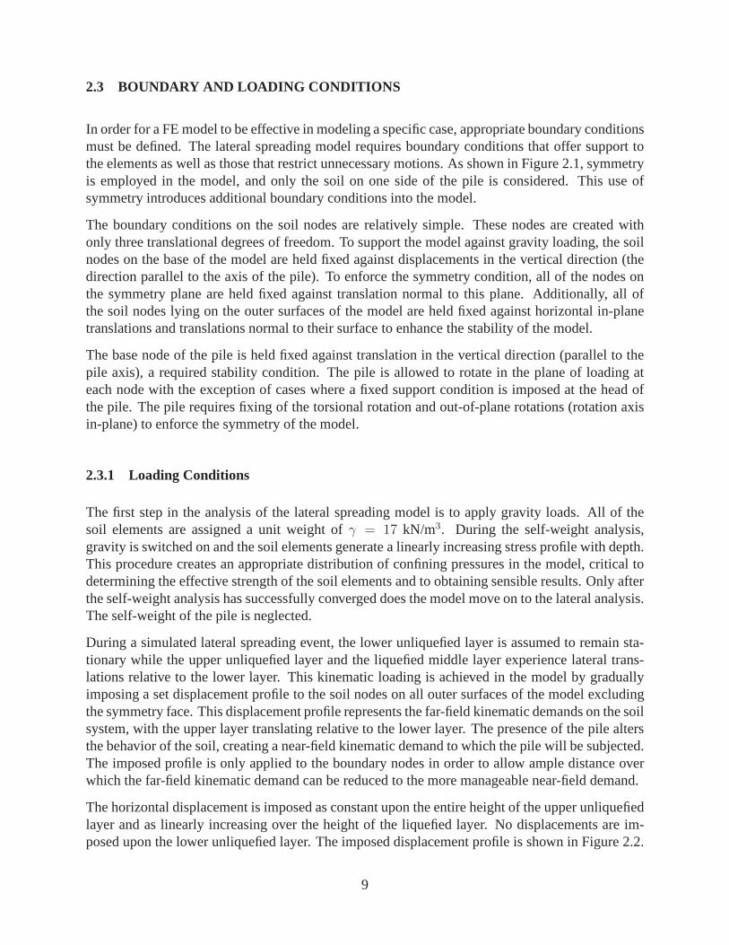
During a simulated lateral spreading event, the lower unliquefied layer is assumed to remain sta-tionary while the upper unliquefied layer and the liquefied middle layer experience lateral trans-lations relative to the lower layer. This kinematic loadingis achieved in the model by graduallyimposing a set displacement profile to the soil nodes on all outer surfaces of the model excludingthe symmetry face. This displacement profile represents thefar-field kinematic demands on the soilsystem, with the upper layer translating relative to the lower layer. The presence of the pile altersthe behavior of the soil, creating a near-field kinematic demand to which the pile will be subjected.The imposed profile is only applied to the boundary nodes in order to allow ample distance overwhich the far-field kinematic demand can be reduced to the more manageable near-field demand.

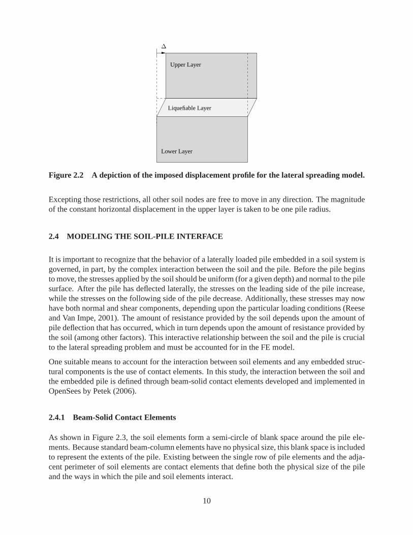
The horizontal displacement is imposed as constant upon theentire height of the upper unliquefiedlayer and as linearly increasing over the height of the liquefied layer. No displacements are im-posed upon the lower unliquefied layer. The imposed displacement profile is shown in Figure 2.2.

9

∆

Liquefiable Layer

Lower Layer

Upper Layer

Figure 2.2 A depiction of the imposed displacement profile for the lateral spreading model.

Excepting those restrictions, all other soil nodes are freeto move in any direction. The magnitudeof the constant horizontal displacement in the upper layer is taken to be one pile radius.

2.4 MODELING THE SOIL-PILE INTERFACE

It is important to recognize that the behavior of a laterallyloaded pile embedded in a soil system isgoverned, in part, by the complex interaction between the soil and the pile. Before the pile beginsto move, the stresses applied by the soil should be uniform (for a given depth) and normal to the pilesurface. After the pile has deflected laterally, the stresses on the leading side of the pile increase,while the stresses on the following side of the pile decrease. Additionally, these stresses may nowhave both normal and shear components, depending upon the particular loading conditions (Reeseand Van Impe, 2001). The amount of resistance provided by thesoil depends upon the amount ofpile deflection that has occurred, which in turn depends uponthe amount of resistance provided bythe soil (among other factors). This interactive relationship between the soil and the pile is crucialto the lateral spreading problem and must be accounted for inthe FE model.

One suitable means to account for the interaction between soil elements and any embedded struc-tural components is the use of contact elements. In this study, the interaction between the soil andthe embedded pile is defined through beam-solid contact elements developed and implemented inOpenSees by Petek (2006).

2.4.1 Beam-Solid Contact Elements

As shown in Figure 2.3, the soil elements form a semi-circle of blank space around the pile ele-ments. Because standard beam-column elements have no physical size, this blank space is includedto represent the extents of the pile. Existing between the single row of pile elements and the adja-cent perimeter of soil elements are contact elements that define both the physical size of the pileand the ways in which the pile and soil elements interact.

10

Figure 2.3 A top view of the finite element mesh for the soil mass. The pile is the dot in thecenter of the lower edge.

(a) (b)

Figure 2.4 Details of the deformation in the soil elements around the pile using beam-solidcontact elements.

The contact element developed by Petek (2006) is formulatedto create a link between the pile,modeled using beam-column elements, and the solid brick elements of the surrounding soil. Theability to use beam-column elements is highly advantageousfrom a modeling standpoint. The con-tact element creates a frictional interface allowing for sticking, slip, and separation that is capableof modeling the coupling between vertical and horizontal displacements. Figure 2.4 provides anexample of how these elements function within the lateral spreading model, showing the way inwhich the soil elements deform around the pile as it moves laterally. The ability of these elementsto create a gap between the trailing edge of the pile and the surrounding soil elements is visibleat the top of Figure 2.4(a). Further information into the development and formulation of thesebeam-to-solid contact elements is available in Petek (2006).

2.5 SURFACE LOAD ELEMENTS

In order to achieve the goals of this research, it is necessary to have models in which the liquefiedlayer is located at varying depths within the soil system. Due to the computational limitations

11

induced by working with 3D FE models, the mesh is selectivelyrefined in the area of the liquefiedlayer as opposed to a uniform refinement. This strategy, while sensible for computational opti-mization, necessitates the creation of customized meshes and input files for each case. In lieu oflaboriously creating a series of models for each pile for liquefied layers at various depths, a uni-form overburden pressure is applied to the ground (free) surface of the soil elements in the model.This overburden pressure, applied as a surface load, creates stress conditions in the soil that areequivalent to moving the liquefied layer to a deeper location.

In OpenSees, there is no built-in surface loading capability, forces can only be applied at a nodallevel. Due to the irregular shape of elements in the lateral spreading model, as shown in Figure 2.3,determination of the equivalent nodal forces for a uniform surface load is a tedious task. One thatwould need to be performed for every increment of overburdenpressure in every model. Instead ofpursuing that strategy for the application of overburden pressure in the FE model, a new elementis developed in OpenSees which is able to determine the appropriate nodal forces for a givenmagnitude of uniform pressure in a quadrilateral element. No additional stiffness is providedby these surface load elements, and the increase in computational cost is minimal, as only theassembly phase is affected. This new element eases the implementation of surface loads for thepurpose of this research, while also increasing the capabilities of the OpenSees platform.

2.5.1 Formulation of Surface Load Elements

The developed surface load element is based upon a relatively simple strategy. The internal forcevector for each element is replaced by the external force vector that would result from the applica-tion of a uniform surface loading. By creating a force imbalance in the elements, for equilibriumto be satisfied there must exist an equal-but-opposite set ofexternal forces applied to each of theelements on the surface. This set of external forces is manifested in the application of energeticallyconjugate nodal forces representing the uniform surface loading.

The formulation of the surface load elements begins with theweak form of the principle of virtualdisplacements

−∫

V

σ : ∇sη dV +

∫

V

b · η dV +

∫

∂Vσ

t · η dS = 0 (2.1)

whereσ is the stress tensor,∇s is the symmetric vector operator,η is an arbitrary displacementfunction,V is the volume of the body,b is the body force acting on the body,t is the surfacetraction vector,∂Vσ is the portion of the surface of the body with prescribed stresses, andS is thesurface of the body.

Equation (2.1) expresses equilibrium for the system in terms of an arbitrary displacement functionη. The vector of external forces, which follows from the thirdterm of Equation (2.1), can bedetermined by, first, expressing the arbitrary displacement as

η =∑

I

NI(ξ, η) · ηI (2.2)

whereNI are the (linear) shape functions, the subscriptI refers to each of the four nodes for theelement, andηI are arbitrary nodal displacements. The shape functions,NI , can be expressed for

12

these quadrilateral elements as

NI =1

4(1 + ξI ξ)(1 + ηI η) (2.3)

by mapping a bi-unit square onto the quadrilateral surface patch. The normalized coordinatesξIandηI represent the nodal coordinates on the bi-unit square.

Applying Equation (2.2) to the external force term of Equation (2.1) results in

∑

I

(∫

t ·NI(ξ, η)Jdξdη

)

· ηI =:∑

I

f extI · ηI (2.4)

which must hold for any arbitrary nodal displacementηI , thus uniquely defining the nodal force

f extI =

∫

t ·NI(ξ, η)Jdξdη (2.5)

whereJ is the Jacobian determinant necessary for the coordinate transformation toξ andη, andthe integration is performed over the bi-unit square to which the element has been mapped.

For a uniform surface pressure applied perpendicular to a given surface, the traction vector,t, is

t = −pn(ξ, η) (2.6)

in which p is the scalar magnitude of the pressure, andn is the unit vector defining the outwardnormal of the surface. To establish the outward normal for the surface elements, general basevectors are defined for each element. There are two general base vectors, one in theξ direction,gξ, and the other in theη direction on the element,gη. This general base can be found from thenodal position vector as

x(ξ, η) =∑

I

NI(ξ, η) · xI (2.7)

wherexI are the nodal position vectors. The base vectors follow as

gξ =∂x

∂ξ=

∑

I

∂NI

∂ξ· xI =

∑

I

ξI4(1 + ηI η) · xI (2.8)

and

gη =∂x

∂η=

∑

I

∂NI

∂η· xI =

∑

I

ηI4(1 + ξI ξ) · xI (2.9)

A local normal vector,̂n, for each element is defined by the cross product of the two base vectorsas

n̂ = gξ × gη (2.10)

This vector contains information about both the area and thedirection of the outward normal for itsrespective element. It can be shown that the norm ofn̂ is equal to the surface Jacobian determinant,J . Thus, the relationship betweenn̂ andn can be expressed as

n =1

Jn̂ (2.11)

13

This relation is used to express the surface traction of Equation (2.6) in terms of the local normalvector as

t = − p

Jn̂ (2.12)

wherep is the magnitude of the surface pressure andJ is the Jacobian determinant.

Applying Equation (2.12) to Equation (2.5), the external force acting at nodeI is obtained as

f extI = −p

∫

n̂(ξ, η)NI(ξ, η)dξdη (2.13)

The integral of Equation (2.13) is evaluated using four-point Gaussian integration of the form

f extI =

2∑

α=1

2∑

β=1

−p n̂(ξα, ηβ)NI(ξα, ηβ)wαwβ (2.14)

in which the Gaussian quadrature and weights are(ξα, wα) = (ηβ, wβ) = (± 1√3, 1).

In each surface element, the internal force vector is set equal to the vector of forces resulting froma uniform surface traction as determined by Equation (2.14). To satisfy equilibrium, the elementsmust be subject to a set of nodal forces in opposition to the prescribed external force.

2.5.2 Validation of Surface Elements

A simple model is created in order to validate the successfulimplementation of the surface loadelements in OpenSees. The model is meshed using irregularly-shaped elements as depicted inFigure 2.5. The newly created surface load elements are applied to the upper surface of this modelover four layers of linear-elastic isotropic brick elements. The irregular shape of the mesh allowsthe elements to be tested for generality, as they should create energetically consistent nodal loadsacross the surface regardless of the shape of the quadrilateral elements, and thus create a constantstress in the solid.

Figure 2.5 Irregularly-shaped mesh used for surface load element validation.

14

−10

−10Vertical stress (kPa)

Figure 2.6 Distribution of vertical stress in the surface load element validation model.

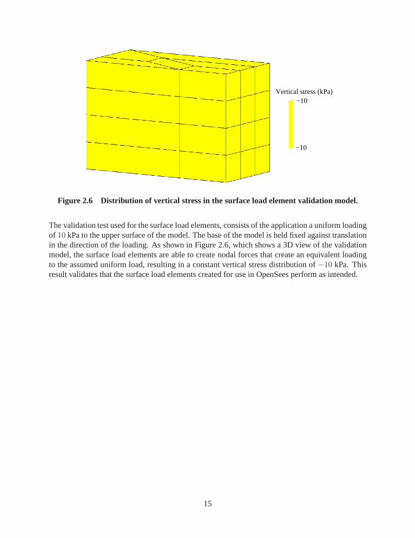
The validation test used for the surface load elements, consists of the application a uniform loadingof 10 kPa to the upper surface of the model. The base of the model is held fixed against translationin the direction of the loading. As shown in Figure 2.6, whichshows a 3D view of the validationmodel, the surface load elements are able to create nodal forces that create an equivalent loadingto the assumed uniform load, resulting in a constant vertical stress distribution of−10 kPa. Thisresult validates that the surface load elements created foruse in OpenSees perform as intended.

15

3 Modeling the Piles

3.1 INTRODUCTION

This study includes three deep foundation models that vary in diameter and bending stiffness. Forsimplicity, the term pile will be used to refer to all foundation elements discussed in the remainderof this report. Each pile model is based upon a template reinforced concrete pile known to havebeen used in practice. All three pile designs are modeled with circular cross sections. The threepiles are selected such that they represent a reasonable variation in size and stiffness; thus providingdata that is relevant to the range of size and stiffness wheremost practical pile designs fall. Thestudy includes a small pile, a mid-sized pile, and a large pile with respective diameters of 0.61 m,1.37 m, and 2.5 m. Both linear elastic and nonlinear elastoplastic constitutive models are createdfor each pile diameter.

3.2 TEMPLATE PILE DESIGNS

Figure 3.1 shows scale section views of the three template piles to emphasize their relative sizes.The majority of piles that are commonly used in practice havecross-sectional areas falling some-where in the range defined by these three piles. Defining a reasonable range of pile sizes encour-ages interpolation of computed results as opposed to extrapolation.

The selected 0.61-m-diameter pile is a design common to the Port of Los Angeles, where piles ofthis type are employed in wharf foundations. This pile is representative of one of the smallest pile

(c)

(b)

(a)

Figure 3.1 Template pile designs (to scale). (a) 0.61-m-diameter; (b) 1.37-m-diameter; (c)2.5-m-diameter.

17

0.686 m 1.25 m1.06 m

casing64 mm

0.313 m0.208 m

@ 76.2 mm9.5 mm ties

16, 15.2 mm dialongitudinal bars

36, 15.2 mm dialongitudinal bars

@ 76.2 mm9.5 mm ties 22.2 mm ties

@ 200 mm

longitudinal bars30, 57.3 mm dia

(c)(b)(a)

0.586 m

Figure 3.2 Dimensions and details of the three template piles. (a) 0.61-m-diameter; (b) 1.37-m-diameter; (c) 2.5-m-diameter.

designs that would commonly be encountered in applicationswhere potentially liquefiable soilsare present. The actual pile design has a 0.61-m-wide octagonal cross section, however, to easeimplementation in the numerical model, a circular cross section is created having an equivalentarea. The amount and location of the longitudinal and spiralreinforcement found in the actualoctagonal pile is left unchanged in the equivalent circularmodel.

A 2.5-m-diameter pile used on the Bay Bridge in the San Francisco Bay is selected to be represen-tative of one of the larger pile designs that would be encountered in practice, thus establishing thehigher end of the range of practical piles. The template 2.5-m-pile is a drilled-shaft, with a steelcasing surrounding an inner core of concrete and reinforcing steel. This casing greatly increasesthe bending stiffness of the 2.5-m-diameter pile as compared to the other selected designs, evenmore so than the increased size.

The third template pile is included to establish an intermediate case. The selected 1.37-m- diameterpile was used on the Dumbarton Bridge (Menlo Park to Fremont,California) replacement project.The actual pile design called for a precast concrete ring, which was to be filled in with a core ofconcrete and reinforcing steel after being driven into place. For ease of modeling, it is assumedthat once the infill has cured, the pile acts as a solid cross section.

A summary of the relevant dimensions and details for each of the three template pile designs isprovided in Figure 3.2. The reinforcing steel layouts shownare incorporated into fiber sectionmodels which simulate the composite behavior of these reinforced concrete piles.

3.3 PILE ELEMENTS

The piles are modeled using beam-column elements with a displacement-based formulation. TheOpenSees designation for the beam-column elements used in the model isdispBeamColumn.These elements are able to include distributed plasticity,and integration within the elements isbased on the Gauss-Legendre quadrature rule. These beam-column elements are used in conjunc-tion with elastic and elastoplastic constitutive formulations incorporated by means of fiber sectionmodels. No geometric nonlinearity is considered. The pile nodes have six degrees of freedom (3translational, 3 rotational).

18

divisionsAngular Radialdivisions

Figure 3.3 Typical fiber discretization for a circular fiber section model.

3.3.1 Fiber Section Models

The three pile designs display differing responses to bending loads based upon the strength, distri-bution, and size of the concrete and steel available in theircross section. In order to incorporate theunique behavior of each pile into a FE model, fiber section models are created for each pile design.These fiber section models incorporate all of the relevant aspects of the template pile designs, anddefine the behavior of each pile model at a cross-sectional level. Due to symmetry considerations,only one-half of each pile is modeled, resulting in semi-circular fiber section models.

Fiber section models are effective when modeling compositematerials such as reinforced concretepiles. Fiber sections have a geometry defined in two levels; an overall geometry, in this case semi-circular, within which exists many smaller subregions of regular shape. A circular shape, or anysector thereof, lends itself well to the discretization framework shown in Figure 3.3 with a set ofdivisions set at even intervals along the radius of the circle, as well as divisions that are set at equalangular increments. Reinforcement steel is included as individual fiber regions with appropriateareas and locations. This type of fiber discretization is employed in all of the fiber models createdfor this research.

Each subregion of the fiber model is assigned its own unique uniaxial constitutive model. Inthe case of reinforced concrete, it follows that the subregions representing the reinforcement aregiven the uniaxial behavior of steel, and the surrounding subregions representing the concreteportion of the cross section are assigned uniaxial constitutive behavior based upon that of concrete.Through defining the fiber model in this manner, a composite constitutive behavior is achievedwhich approximates the 3D behavior of an actual pile while still enabling the use of standard beamelements.

19

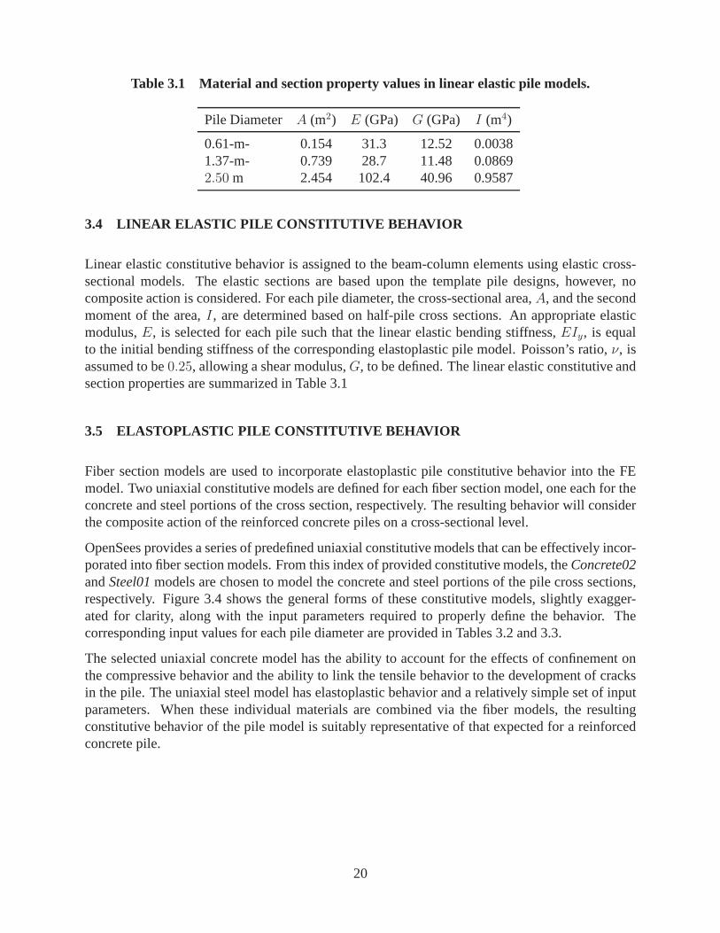
Table 3.1 Material and section property values in linear elastic pile models.

Pile Diameter A (m2) E (GPa) G (GPa) I (m4)

0.61-m- 0.154 31.3 12.52 0.00381.37-m- 0.739 28.7 11.48 0.08692.50 m 2.454 102.4 40.96 0.9587

3.4 LINEAR ELASTIC PILE CONSTITUTIVE BEHAVIOR

Linear elastic constitutive behavior is assigned to the beam-column elements using elastic cross-sectional models. The elastic sections are based upon the template pile designs, however, nocomposite action is considered. For each pile diameter, thecross-sectional area,A, and the secondmoment of the area,I, are determined based on half-pile cross sections. An appropriate elasticmodulus,E, is selected for each pile such that the linear elastic bending stiffness,EIy, is equalto the initial bending stiffness of the corresponding elastoplastic pile model. Poisson’s ratio,ν, isassumed to be0.25, allowing a shear modulus,G, to be defined. The linear elastic constitutive andsection properties are summarized in Table 3.1

3.5 ELASTOPLASTIC PILE CONSTITUTIVE BEHAVIOR

Fiber section models are used to incorporate elastoplasticpile constitutive behavior into the FEmodel. Two uniaxial constitutive models are defined for eachfiber section model, one each for theconcrete and steel portions of the cross section, respectively. The resulting behavior will considerthe composite action of the reinforced concrete piles on a cross-sectional level.

OpenSees provides a series of predefined uniaxial constitutive models that can be effectively incor-porated into fiber section models. From this index of provided constitutive models, theConcrete02andSteel01models are chosen to model the concrete and steel portions ofthe pile cross sections,respectively. Figure 3.4 shows the general forms of these constitutive models, slightly exagger-ated for clarity, along with the input parameters required to properly define the behavior. Thecorresponding input values for each pile diameter are provided in Tables 3.2 and 3.3.

The selected uniaxial concrete model has the ability to account for the effects of confinement onthe compressive behavior and the ability to link the tensilebehavior to the development of cracksin the pile. The uniaxial steel model has elastoplastic behavior and a relatively simple set of inputparameters. When these individual materials are combined via the fiber models, the resultingconstitutive behavior of the pile model is suitably representative of that expected for a reinforcedconcrete pile.

20

(εc, f ′

c)

σ

Et

ft

ε

(εcu, f ′

cu)

Ec = 2f ′

c

εc

σ

σy

-σy

Es

ε

bEs

(a) (b)

Figure 3.4 Uniaxial constitutive relations used in fiber section models. (a) Concrete02model. (b)Steel01model.

Table 3.2 Steel material property input values in fiber section models.

Pile Diameter σy (MPa) Es (GPa) b

0.61-m- 1860 200 0.0011.37-m- 1860 200 0.0012.50 m 520 200 0.001

Table 3.3 Concrete material property input values in fiber section models.

Pile Diameter f ′

c (kPa) εc f ′

cu (kPa) εcu ft (kPa) Et (MPa)

0.61-m- 44816 0.003 8960 0.015 4170 -20801.37-m- 43170 0.003 8270 0.011 4000 -14002.50 m 20684 0.003 4140 0.013 2830 -13800

21

3.5.1 Steel in Tension and Compression

The chosen uniaxial steel material model, while not intended solely for use in reinforcement mod-eling, has many of the salient features that are desirable ina steel constitutive model. As shownin Figure 3.4(b), theSteel01model is a bilinear plasticity model that incorporates isotropic strainhardening in the post-yield behavior. The initial portion of the model is linear elastic, with a slopedefined by the modulus of elasticity,E. The hardening slope of the curve is defined as the productof the elastic modulus and a specified hardening ratio,b, which was taken as a somewhat arbitraryvalue of0.001. Although this constitutive model is relatively simple, the bilinear model createsa situation in which there is a constant tangent in the plastic region, thus, simplifying the com-putations without significantly affecting the results. Thelongitudinal reinforcement fibers in allthree pile models, as well as the steel tube in the 2.5-m-pilemodel, are defined using this uniaxialconstitutive model.

3.5.2 Concrete in Compression

In compression, the selected uniaxial concrete constitutive model is based upon the work of Kentand Park (1971), who derived the model from tests conducted with confined concrete beam-columns. This model has three distinct regions of behavior that define the initial, crushing, andpost-crushing relationships between the axial stress and strain in each subregion of the fiber ele-ments. Whenever possible, the material parameters used as input values in the constitutive modelsare based on the corresponding properties in the template pile designs.

In the initial loading region, from the origin up to the maximum compressive stress and strain,the behavior is parabolic. The maximum strength in compression, f ′

c, for each model was takendirectly from the template pile designs (see Table 3.3 for values). Per American Concrete Institute(ACI) recommendations, all three piles are assumed to have apeak strain ofεc = 0.003 when theirmaximum compressive stress has been reached (ACI, 2005). The initial tangent of this region ofthe model is equal to the modulus of elasticity,E, which is defined as

E = 2f ′

c

εc(3.1)

Once the strain in the model exceeds the set value ofεc, the concrete begins to soften due to theonset of crushing. This is represented by the descending linear region of the material behaviorshown in Figure 3.4(a). The speed at which this softening occurs is based upon the amount ofconfinement provided by the longitudinal bars and spiral ties included in the cross section. Withgreater levels of confinement, larger axial strains can be achieved in the concrete core before thecontribution of that concrete to the strength of the pile becomes minimal. To account for theinfluence of the amount of confinement in each pile model, the post-crushing behavior for therespective concrete constitutive models are defined in accordance with a procedure detailed in Parkand Paulay (1975). Using this procedure,εcu, the strain at which the concrete is considered entirelycrushed, can be defined based upon the known geometry of the core and the amount of steel bywhich it is confined. The crushed strains for each model are provided in Table 3.3.

22

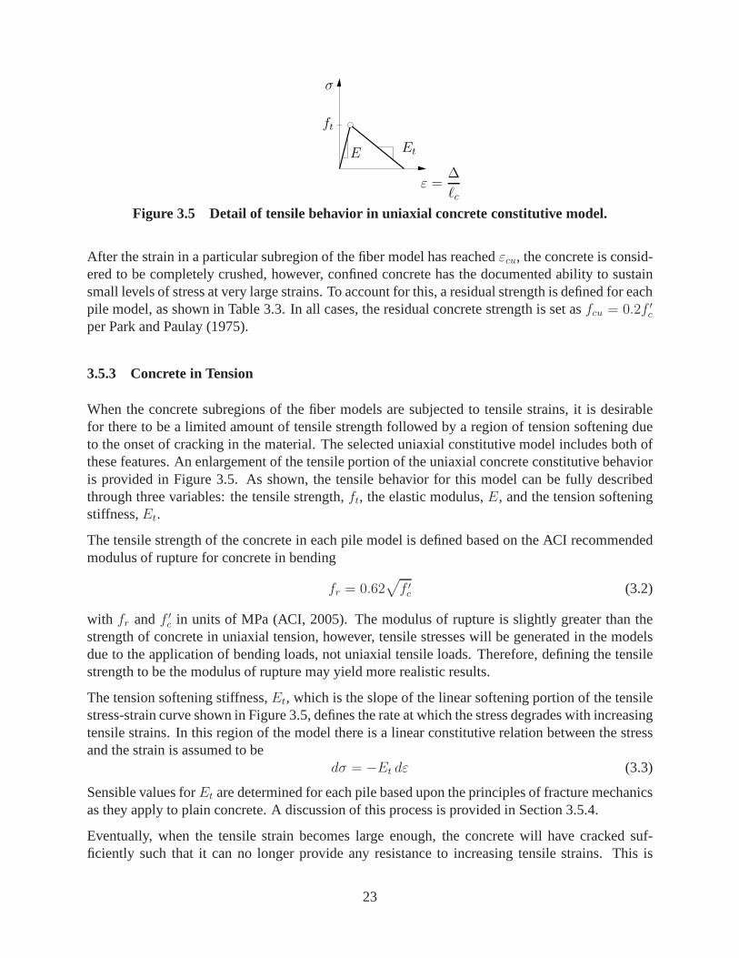
ft

σ

EtE

ε =∆

ℓc

Figure 3.5 Detail of tensile behavior in uniaxial concrete constitutive model.

After the strain in a particular subregion of the fiber model has reachedεcu, the concrete is consid-ered to be completely crushed, however, confined concrete has the documented ability to sustainsmall levels of stress at very large strains. To account for this, a residual strength is defined for eachpile model, as shown in Table 3.3. In all cases, the residual concrete strength is set asfcu = 0.2f ′

c

per Park and Paulay (1975).

3.5.3 Concrete in Tension

When the concrete subregions of the fiber models are subjected to tensile strains, it is desirablefor there to be a limited amount of tensile strength followedby a region of tension softening dueto the onset of cracking in the material. The selected uniaxial constitutive model includes both ofthese features. An enlargement of the tensile portion of theuniaxial concrete constitutive behavioris provided in Figure 3.5. As shown, the tensile behavior forthis model can be fully describedthrough three variables: the tensile strength,ft, the elastic modulus,E, and the tension softeningstiffness,Et.

The tensile strength of the concrete in each pile model is defined based on the ACI recommendedmodulus of rupture for concrete in bending

fr = 0.62√

f ′

c (3.2)

with fr andf ′

c in units of MPa (ACI, 2005). The modulus of rupture is slightly greater than thestrength of concrete in uniaxial tension, however, tensilestresses will be generated in the modelsdue to the application of bending loads, not uniaxial tensile loads. Therefore, defining the tensilestrength to be the modulus of rupture may yield more realistic results.

The tension softening stiffness,Et, which is the slope of the linear softening portion of the tensilestress-strain curve shown in Figure 3.5, defines the rate at which the stress degrades with increasingtensile strains. In this region of the model there is a linearconstitutive relation between the stressand the strain is assumed to be

dσ = −Et dε (3.3)

Sensible values forEt are determined for each pile based upon the principles of fracture mechanicsas they apply to plain concrete. A discussion of this processis provided in Section 3.5.4.

Eventually, when the tensile strain becomes large enough, the concrete will have cracked suf-ficiently such that it can no longer provide any resistance toincreasing tensile strains. This is

23

w

σ

ft

Et

Gf

ft

Et

Figure 3.6 Simplified fracture model for concrete in uniaxial tension.

represented in Figure 3.5 by the point at which the softeningcurve crosses the strain axis. Thislimiting value of strain varies for each model based upon their respective tensile strengths andsoftening moduli.

3.5.4 One-Dimensional Fracture Mechanics of Concrete in Tension

When concrete approaches its tensile capacity, defined in this model by the modulus of rupture,cracks will begin to form. Though the cracks may propagate relatively rapidly, the surroundingconcrete does not lose all tensile strength instantaneously. Instead, the tensile stress in the regionof the crack is assumed to degrade over time as a function of the width of the crack opening,w.The rate at which this occurs varies depending upon the material in question.

Models of varying levels of complexity have been developed to describe the relationship betweenthe tensile stress and the rate at which cracks will open in a material, (e.g. Kaplan, 1961; Bazantand Becq-Giraudon, 2002; Xu and Zhang, 2008). For the purposes of this research, a simplifiedcrack propagation model has been adopted. This model is shown in Figure 3.6, where the tensilestress is plotted as a linear function of the crack opening. This assumed relationship betweenincremental stresses and crack widths is defined by the crackpropagation slope,Et, and can bewritten as

dσ = −Et dw (3.4)

an expression that is helpful in relatingEt to the desired input value ofEt.

As shown in Figure 3.6, there is a certain amount of energy that must be expended before theconcrete in the area of the crack loses its tensile strength entirely. This energy is called the fractureenergy, or fracture toughness, and is commonly denoted asGf . Fracture energy is a fundamentalmaterial property that can be determined via laboratory tests or from empirical formulas presentin the literature. The fracture energy for each pile model isdefined as shown in Table 3.4; valuesdetermined using the empirical procedure developed by Bazant and Becq-Giraudon (2002).

In a general sense, the value of the fracture energy for a given material is dependent upon thespecific relationship between the tensile stress and the crack opening width, defined by the functionσ(w). The fracture energy is equal to the following integral

Gf =

∫ +∞

0

σ(w) dw (3.5)

24

Table 3.4 Concrete fracture energies and crack propagationslopes.

Pile Diameter Gf (kJ/m2) Et (MN/m3)

0.61-m- 0.155 554501.37-m- 0.150 531002.50 m 0.109 36520

which essentially states thatGf is equal to the area under the curve defined byσ(w). Applyingthis to the simplified model shown in Figure 3.6, the fractureenergy can be related to the tensilestress at the onset of cracking,ft, and the crack propagation rate,Et, as

Gf =1

2ftw

=f 2t

2Et

(3.6)

Solving Equation (3.6) for the unknown crack propagation slope results in

Et =f 2t

2Gf(3.7)

which definesEt in terms of the known values for concrete fracture energy andtensile strength.The values ofEt calculated for each pile diameter are summarized in Table 3.4.

A consideration of what is happening in a single pile elementduring cracking is beneficial whenattempting to relate the stress degradation slope,Et, to the tension softening slope,Et. Figure 3.7shows such an element both before (w = 0) and after (w > 0) the onset of cracking. For simplicityit is common to assume that there is a single crack in each element that occurs at the midpoint of itslength. This assumption defines the characteristic length,ℓc, which is the distance between cracks,to be equal to the element length.

w

ℓc

∆

∆

ε = ∆ℓc

Figure 3.7 Relationship between elongation, crack width, and element length for a singlepile element.

25

The change in length of the element,d∆, can be related to the change in strain within the element,dε by the simple kinematic relation

d∆ = ℓc dε (3.8)

As implied by Figure 3.7, the addition of a crack with increasing width into the element modifiesEquation (3.8) into the form

d∆ = ℓc dεe + dw (3.9)

wheredεe is the change in elastic strain anddw is the change in crack opening width. Assuminglinear elastic behavior in the uncracked zone, Equation (3.9) can be written in terms of stress as

d∆ =ℓcEdσ + dw (3.10)

in which E is the elastic modulus. Expanding Equation (3.10) using Equations (3.4) and (3.8)yields

(

1− ℓcEt

E

)

dw = ℓc dε (3.11)

which can be solved for the incremental change in crack width, yielding

dw =ℓc

(

1− Et ℓcE

)dε (3.12)

The constitutive relation defining the behavior of the tension-softening portion of the concretemodel follows from Equations (3.4) and (3.12) as

dσ = − Et ℓc(

1− Et ℓcE

)dε (3.13)

which when compared with Equation (3.3) defines the tension softening modulus to be

Et =Et ℓc

(

1− Et ℓcE

)(3.14)

This result, combined with Equation (3.7), enables the calculation of the tension softening modulusfor any finite element discretization using known material parameters and element sizes.

3.5.5 Implementation of Tension Parameters

The resultant tension softening modulus from Equation (3.14) is largely dependent upon the chosencharacteristic length,ℓc. The other terms are material-dependent parameters, but the characteristiclength is somewhat arbitrary. As was discussed previously,ℓc is initially taken to be equal tothe element length, thus implying that a single crack develops in each element. As the lengthof an element increases, this assumption becomes less valid. Assuming that there is an adequate

26

Table 3.5 Characteristic length and tension softening modulus in pile models.

Pile Diameter ℓc (m) Et (kPa)

0.61-m- 0.07 -2.08e61.37-m- 0.05 -1.40e62.50 m 0.42 -1.38e7

amount of longitudinal and shear reinforcement provided ina pile, it could be expected for cracksto develop at spacings in the range of5-10 cm. Specifyingℓc to be equal to the expected crackspacing can reduceEt considerably. Reducing the tension softening modulus can result in modelsthat exhibit fewer convergence issues without altering theresults in a significant manner.

Preliminary sensitivity studies performed with the three pile models have shown that the 0.61-mand 1.37-m-diameter models are very sensitive to the specified input value forEt. In these models,there is a significant reduction in stiffness when the concrete cracks in tension. IfEt is set at toolarge a value, the resulting softening behavior is too steepand the elements are unable to converge.An example of this severe softening behavior can be seen inside the circled region of the moment-curvature response shown in Figure 3.8. The convergence issues encountered for these two pilemodels identified the need for a more careful selection of thecharacteristic length values.

Because the 2.5-m-diameter model is encased in a steel tube,it does not display a similar lossof strength at the onset of tension cracking. This is illustrated by Figure 3.9, which shows themoment-curvature behavior for the 2.5-m-diameter cross section for two extreme values ofℓc.There is no discernable difference, thus the characteristic length and the corresponding tensionsoftening stiffness can be set at any sensible value.

Characteristic lengths ofℓc = 7 cm andℓc = 5 cm are selected for the 0.61-m and 1.37-m-diameter models, respectively. For the 2.5-m-diameter model, ℓc is set as the length of the smallestpile element. Table 3.5 summarizes the characteristic length and softening stiffness values.

As shown in Figures 3.10 and 3.11, reducing the tension softening modulus for the 0.61-m and1.37-m-diameter models results in a smoother transition between the initial and ultimate behaviorof the cross section, and the convergence issues associatedwith a large tension softening stiffnessdisappear. The validation work performed in order to support the reduction in these parameters isdiscussed in Section 3.6.2.

27

0 0.01 0.02 0.03 0.04 0.05 0.06 0.07 0.08 0.090

100

200

300

400

500

600

700

800

900

1000

Curvature (m−1)

Mom

ent

(kN

−m

)

Figure 3.8 Moment-curvature behavior for 0.61-m-diametermodel illustrating softeningbehavior resulting from a large characteristic length,ℓc.

0 0.005 0.01 0.015 0.02 0.0250

0.5

1

1.5

2

2.5x 10

5

Curvature (m−1)

Mom

ent

(kN

−m

)

characteristic length = largest elementcharacteristic length = smallest element

Figure 3.9 Moment-curvature behavior for 2.5-m-diameter model with two values of char-acteristic length,ℓc.

28

0 0.02 0.04 0.06 0.08 0.10

100

200

300

400

500

600

700

800

900

1000

Curvature (m−1)

Mom

ent

(kN

−m

)

characteristic length = 0.07 mcharacteristic length = largest elementcharacteristic length = smallest element

Figure 3.10 Moment-curvature behavior for 0.61-m-diameter model with various values ofℓc. Largest element length is0.649 m. Smallest element length is0.102 m.

0 0.005 0.01 0.015 0.02 0.025 0.03 0.035 0.04 0.0450

1000

2000

3000

4000

5000

6000

Curvature (m−1)

Mom

ent

(kN

−m

)

characteristic length = 0.05 mcharacteristic length = largest elementcharacteristic length = smallest element

Figure 3.11 Moment-curvature behavior for 1.37-m-diameter model with various values ofℓc. Largest element length is1.79 m. Smallest element length is0.231 m.

29

3.6 VALIDATION OF PILE MODELS

In all computer simulations, it is important to ensure that user-created models exhibit reasonablebehavior in response to easily verifiable loading conditions. Each step in the creation of the pilemodels, from the behavior of the cross section to the overallbehavior model, must first be validatedbefore implementation into the lateral spreading model.

To ensure that the fiber section models for each pile are created and implemented correctly, thebehavior of each is evaluated and verified through a series ofsimple analyses. The first step isto verify the moment-curvature relation for each fiber model, thus providing reassurance that themodels are created properly. Once this has been established, a cantilever beam model is imple-mented to test the global behavior of the pile models. Unlessotherwise noted, all of the fibersection validation work is performed using the half-pile fiber section models created for use in thelateral spreading model.

3.6.1 Moment-Curvature Response

Using OpenSees, zero-length element models are created with the previously defined semi-circularfiber section models. One node is held fixed, and the other is left free with respect to rotation. Theelement is then subjected to, first, a constant axial load to represent the self weight of the pile, andsecond, a linearly-increasing applied moment. The force and deformation responses of the sectionare recorded during this process, from which a moment-curvature diagram can be created. Thisprocedure is a relatively simple way to establish the moment-curvature behavior for a fiber sectionmodel in OpenSees.

Computer aided hand-calculations are performed to verify that the correct initial tangents and thetrue moment-curvature behaviors of the cross section have been captured in the OpenSees analy-sis. These calculations are implemented in MATLAB and utilize a numeric integration algorithmin combination with a Newton-Raphson iterative procedure.Computing the moment-curvatureresponse of a cross section requires iteratively solving the following equation

R =

{

N −∫

AσdA

M −∫

AyσdA

}

= 0 (3.15)

whereR is the residual,N is the applied normal force,M is the applied moment,σ is the axialstress,A is the area of the cross section, andy is distance from the neutral axis. Incrementalchanges in the residual are computed using the following equation

dR =

[

−∫

∂σ/∂ε −∫

∂σ/∂φ−∫

y∂σ/∂ε −∫

y∂σ/∂φ

]

(3.16)

in which ε is the axial strain andφ is the curvature. The curvature is increased incrementallyin constant steps towards a pre-defined ultimate value. For each curvature step, the axial straindistribution in the cross section can be computed as

ε(y) = εcurrent+ φy (3.17)

30

whereε(y) is the axial strain as a function of positiony, φ is the curvature at the current step,andεcurrent is the mean axial strain at the beginning of each iteration. The distributions of stressresulting from this computed strain distribution are calculated using the appropriate constitutivemodels for the concrete and steel portions of the cross section.

The cross section is divided into subregions. Rectangular and circular subregions are used for theconcrete and steel portions of the cross section, respectively. Each subregion has a particular centerposition,yi, and area,Ai. Using these subregions, the internal normal force and moment acting onthe cross section can be approximated using the following sums

∫

A

σdA ≈∑

σiAi (3.18)

∫

A

yσdA ≈∑

yiσiAi (3.19)

whereσi is the stress acting at the center of each ofi subregions. Additionally, the terms ofEquation (3.16) are computed as

∫

∂σ

∂ε≈

∑

EcAci + EsAsi (3.20)

∫

∂σ

∂φ≈

∑

EcyciAci + EsysiAsi (3.21)

∫

y∂σ

∂ε≈

∑

EcyciAci + EsysiAsi (3.22)

∫

y∂σ

∂φ≈

∑

EcIci + EsIsi (3.23)

in whichEc, yci, andAci are the concrete elastic modulus and the center location andarea for eachconcrete subregion, respectively, andEs, ysi, andAsi are the corresponding terms for the steelportion of the cross section.

The internal normal force and moment obtained from Equations (3.18) and (3.19) are used to com-pute the residual using Equation (3.15). If the residual is not a zero vector, an updated strain distri-bution is computed using the newly computed residual and theincremental change in the residualdetermined in Equations (3.20)–(3.23). The process then repeats, iterating until Equation (3.15)is satisfied for the current curvature step before moving on to the next. The moment-curvatureresponse of the cross section is determined by recording theconverged values of the moment foreach curvature step.

The converged final stress and strain distributions acting over the cross section are recorded andshown in Figure 3.12 for the 0.61-m-diameter section. The similarity to the specified uniaxialsteel and concrete constitutive models shown in Figure 3.4 verifies that the constitutive models arecorrectly implemented in the independent calculation procedure.

The moment-curvature response of each pile model obtained from OpenSees is compared to thecorresponding response computed using the developed MATLAB scheme in Figures 3.13 to 3.18.

31

−0.05 0 0.05−0.3

−0.2

−0.1

0

0.1

0.2

0.3

Strain

Pos

ition

(m

)

−50 0 50−0.3

−0.2

−0.1

0

0.1

0.2

0.3

Concrete stress (MPa)−2000 0 2000

−0.3

−0.2

−0.1

0

0.1

0.2

0.3

Steel stress (MPa)

SteelCompression

CrackedConcrete

Tension steelyielding

CompositeNeutral Axis

Figure 3.12 Distributions of stress and strain determined for 0.61-m-diameter cross section.

Calculations are conducted for full, circular fiber models in addition to the semi-circular sectionmodels developed for use in the 3D lateral spreading model. As shown, there is considerableagreement between the independently calculated and OpenSees curves for each model; the generalshapes are nearly identical and the calculated initial tangents match the OpenSees results. Anydifferences can be attributed to the differing degrees of accuracy in the discretization of the crosssections. These analyses provide verification that the fibermodels are displaying predictable andintended responses as implemented in OpenSees.

The circular cross sections are analyzed in order to verify that the semi-circular fiber section modelshave been correctly implemented. The resulting pile moments and forces in the lateral spreadingmodel should be half as large as would be expected for the fullcross sections due to symmetryconsiderations. The semi-circular models (Figures 3.14, 3.16, and 3.18) display moments whichare exactly one-half of those returned by the circular models for a given curvature value. Thisverifies the correct implementation of the semi-circular fiber section models.

32

0 0.02 0.04 0.06 0.08 0.10

100

200

300

400

500

600

700

800

900

1000

Curvature (m−1)

Mom

ent

(kN

−m

)

OpenSeesMatlabInitial Tangent

Figure 3.13 Comparison of moment-curvature responses for 0.61-m-diameter full (circu-lar) pile model.

0 0.02 0.04 0.06 0.08 0.10

50

100

150

200

250

300

350

400

450

500

Curvature (m−1)

Mom

ent

(kN

−m

)


Figure 3.14 Comparison of moment-curvature responses for 0.61-m-diameter half-pile(semi-circular) model.

33

0 0.005 0.01 0.015 0.02 0.025 0.03 0.035 0.040

1000

2000

3000

4000

5000

6000

7000

Curvature (m−1)

Mom

ent

(kN

−m

)


Figure 3.15 Comparison of moment-curvature responses for 1.37-m-diameter full (circu-lar) pile model.

0 0.005 0.01 0.015 0.02 0.025 0.03 0.035 0.040

500

1000

1500

2000

2500

3000

3500

Curvature (m−1)

Mom

ent

(kN

−m

)



34

0 0.005 0.01 0.015 0.02 0.0250

0.5

1

1.5

2

2.5x 10

5

Curvature (m−1)

Mom

ent

(kN

−m

)


Figure 3.17 Comparison of moment-curvature responses for 2.5-m-diameter full (circular)pile model.

0 0.005 0.01 0.015 0.02 0.0250

5

10

15x 10

4

Curvature (m−1)

Mom

ent

(kN

−m

)



35

PD

R

L= 21D

Figure 3.19 Cantilever beam analysis. The horizontal load,P, is increased linearly until thepile tip deflects a distance of one pile radius.

Cantilever Beam Implementation

In order to ensure that the behavior of the section models is consistent regardless of the loadingconfiguration, a simple cantilever beam model is used. A schematic of this model is provided inFigure 3.19. The cantilever beams utilize the fiber section models for each pile. The moment-curvature responses for the 0.61-m and 2.5-m-diameter piles in the element adjacent to the fixedbase are compared to previous results in Figures 3.20 and 3.21. The similarity shown providesverification that the cross-sectional model can be successfully implemented into a 3D simulation.

3.6.2 Validation of Tension Parameters

As discussed in Section 3.5.5, the 0.61-m-and 1.37-m-diameter models exhibit convergence prob-lems when assigned large values of the tension softening modulus,Et. While it is important toselect input parameters that allow for convergence, it is equally important to validate that anychanges in the parameters are sensible and do not significantly alter the resulting behavior of thepile models. To show that a suitable compromise between accuracy/detail resolution and numericalstability in the tension softening parameter does not significantly affect the results, the behavior ofthe pile models for several values ofEt is compared via two validation studies.

In the first validation study, the moment-curvature behavior of the pile models is compared for threeseparate values ofEt. This behavior is generated for each model using the zero-length elementapproach discussed in Section 3.6.1. Two of the three tension softening stiffness values are basedupon characteristic lengths set equal to the sizes of the largest and smallest elements, respectively,in each pile model. These characteristic lengths derive from the assumption that a single crackdevelops in each element. The third value ofEt is determined by setting the characteristic lengthto be the assumed crack spacings listed in Table 3.5.

For the lateral spreading model, it is important that the behavior of the pile elements at large curva-ture and displacement demands remains unaffected by changes in the tension softening modulus.Part of the goal of this research is to evaluate the maximum moments, shear forces, and curvatures

36

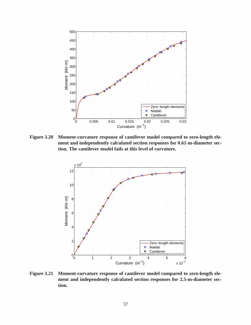
0 0.005 0.01 0.015 0.02 0.025 0.030

50

100

150

200

250

300

350

400

450

500

Curvature (m−1)

Mom

ent

(kN

−m

)

Zero−length elementsMatlabCantilever

Figure 3.20 Moment-curvature response of cantilever modelcompared to zero-length ele-ment and independently calculated section responses for 0.61-m-diameter sec-tion. The cantilever model fails at this level of curvature.

0 1 2 3 4 5 6

x 10−3

0

2

4

6

8

10

12

x 104

Curvature (m−1)

Mom

ent

(kN

−m

)

Zero−length elementsMatlabCantilever

Figure 3.21 Moment-curvature response of cantilever modelcompared to zero-length ele-ment and independently calculated section responses for 2.5-m-diameter sec-tion.

37

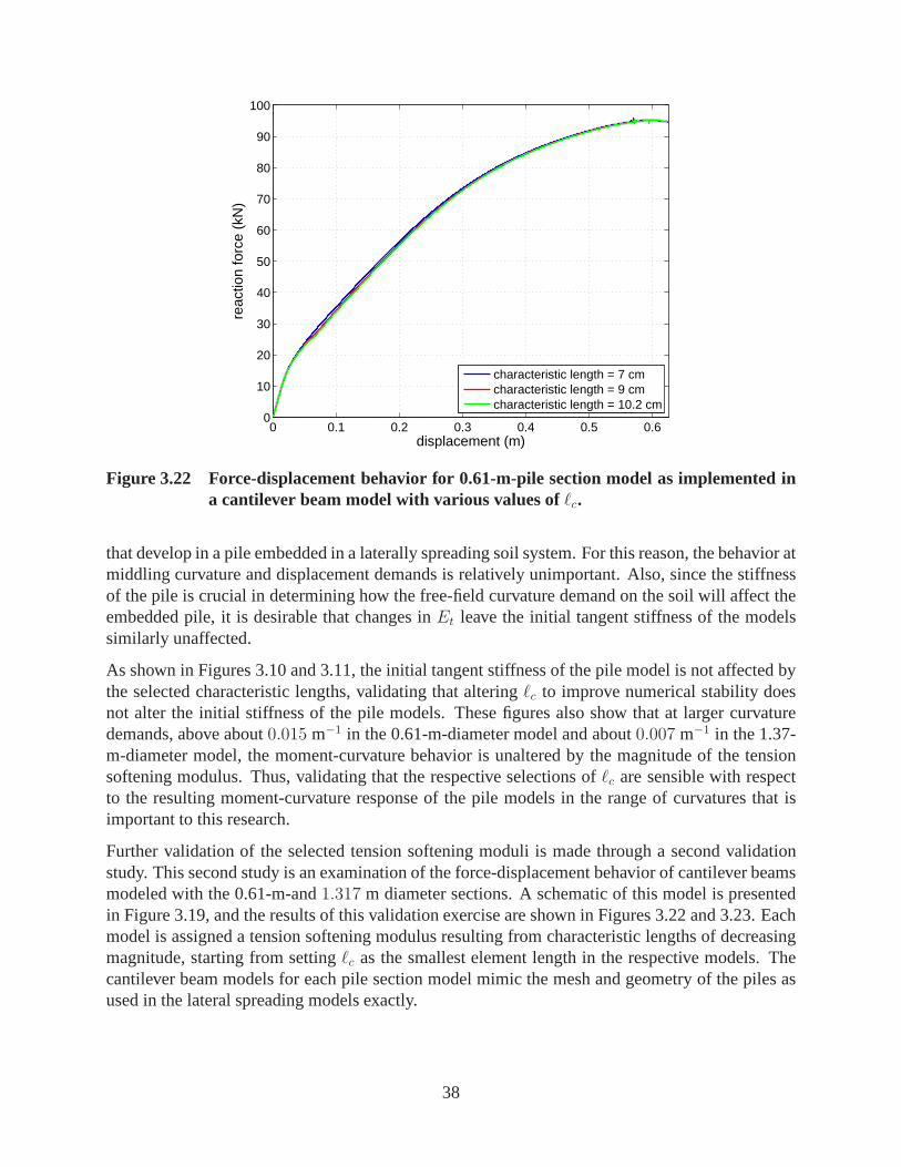
0 0.1 0.2 0.3 0.4 0.5 0.60

10

20

30

40

50

60

70

80

90

100

displacement (m)

reac

tion

forc

e (k

N)

characteristic length = 7 cmcharacteristic length = 9 cmcharacteristic length = 10.2 cm

Figure 3.22 Force-displacement behavior for 0.61-m-pile section model as implemented ina cantilever beam model with various values ofℓc.

that develop in a pile embedded in a laterally spreading soilsystem. For this reason, the behavior atmiddling curvature and displacement demands is relativelyunimportant. Also, since the stiffnessof the pile is crucial in determining how the free-field curvature demand on the soil will affect theembedded pile, it is desirable that changes inEt leave the initial tangent stiffness of the modelssimilarly unaffected.

As shown in Figures 3.10 and 3.11, the initial tangent stiffness of the pile model is not affected bythe selected characteristic lengths, validating that altering ℓc to improve numerical stability doesnot alter the initial stiffness of the pile models. These figures also show that at larger curvaturedemands, above about0.015 m−1 in the 0.61-m-diameter model and about0.007 m−1 in the 1.37-m-diameter model, the moment-curvature behavior is unaltered by the magnitude of the tensionsoftening modulus. Thus, validating that the respective selections ofℓc are sensible with respectto the resulting moment-curvature response of the pile models in the range of curvatures that isimportant to this research.

Further validation of the selected tension softening moduli is made through a second validationstudy. This second study is an examination of the force-displacement behavior of cantilever beamsmodeled with the 0.61-m-and1.317 m diameter sections. A schematic of this model is presentedin Figure 3.19, and the results of this validation exercise are shown in Figures 3.22 and 3.23. Eachmodel is assigned a tension softening modulus resulting from characteristic lengths of decreasingmagnitude, starting from settingℓc as the smallest element length in the respective models. Thecantilever beam models for each pile section model mimic themesh and geometry of the piles asused in the lateral spreading models exactly.

38

0 0.2 0.4 0.6 0.8 1 1.2 1.40

50

100

150

200

250

300

displacement (m)

reac

tion

forc

e (k

N)

characteristic length = 5 cmcharacteristic length = 9 cmcharacteristic length = 18 cmcharacteristic length = 23.1 cm

Figure 3.23 Force-displacement behavior for 1.37-m-pile section model as implemented ina cantilever beam model with various values ofℓc.

The effects of the changes in magnitude of the tension softening parameter are more apparent inthe cantilever model, where the elements have lengths, as compared to the zero-length elementapproach used to generate the moment-curvature behavior ofthe models. This is demonstrated bythe observation that the cantilever models for both pile models are unable to converge past a fewtime steps when the characteristic length is set as the largest element length. Once the tensile stressin the cross section reaches that which signals the onset of cracking, no converged solution can befound. The models display convergence issues even whenℓc is set as the smallest element length,though, unlike the case where the characteristic length is equal to the largest element length, themodels will converge, albeit with a large number of small load steps. As in the moment-curvaturestudy, the initial behavior is the same regardless of parameter selection, and all of the cases reachessentially the same reaction force at the final displacement.

The selections ofℓc summarized in Table 3.5, and the resulting tension softening moduli are madewith consideration towards a realistic crack spacing as well as with respect to the convergence be-havior of the pile models. The cantilever verification studyvalidates that the selected characteristiclength parameter will allow the pile models to reach convergence when implemented in a modelwith actual geometry, validation that the zero-length elements cannot provide. Additionally, thecantilever study demonstrates that the magnitude of the tension softening modulus only affects themiddle range of the models’ behavior; the initial and final ranges are unaffected.

39

4 Modeling the Soil

4.1 INTRODUCTION

The behavior of the soil surrounding the piles is important to the problem of a pile embedded inlaterally spreading soils as it is both the source of and the medium through which the kinematicdemands of the moving soil mass are transmitted to the embedded pile foundations. In the layeredsoil system considered in this study, the thickness of the liquefied layer and the various materialproperties of the surrounding soil layers are integral to defining how a pile experiences a lateralspreading event. Seemingly minor changes in the material properties or the configuration of thelayers can significantly alter the resultant behavior of an embedded pile. In order for the results ofthis study to be valid for most piles in different soils, it iscritical to select appropriate values forthe soil parameters.

The typical considered soil system consists of three individual soil layers modeled as a 3D con-tinuum surrounding the pile. A global view of the complete FEmodel is shown in Figure 2.1, inwhich the various soil layers and the general layout of the soil elements are clearly visible. Soilmodeling decisions are made based upon the assumption that all three layers are made up entirelyof homogenous (within each layer) cohesionless soil.

Two separate soil constitutive models are considered. One of these models considers the soil to belinear elastic while the other soil model considers elastoplastic behavior using a Drucker-Pragerconstitutive model developed and implemented for use in OpenSees (Petek, 2006).

4.2 SOIL ELEMENTS

The soil continuum is modeled using eight-node brick elements. The soil nodes defining theseelements are created with three translational degrees of freedom. The number of soil elementsranges from2720 to 3360 depending upon pile diameter considered in each particularcase. Thedegree of mesh refinement is increased in the middle of the model as compared to the regions nearthe top and bottom of the model. This meshing scheme allows the areas of importance, i.e. theareas near the liquefied interface, to have a relatively fine mesh, while leaving the outlying regionswith a coarser level of refinement.

Unless otherwise noted, the elements of all three soil layers are assigned a unit weight,γ =17 kN/m3, which is typical for most soil conditions. The first step in the lateral spreading analysis

41

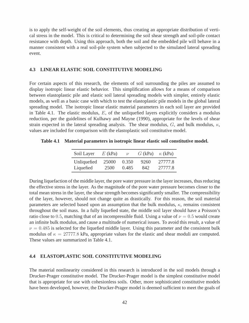
is to apply the self-weight of the soil elements, thus creating an appropriate distribution of verti-cal stress in the model. This is critical to determining the soil shear strength and soil-pile contactresistance with depth. Using this approach, both the soil and the embedded pile will behave in amanner consistent with a real soil-pile system when subjected to the simulated lateral spreadingevent.

4.3 LINEAR ELASTIC SOIL CONSTITUTIVE MODELING

For certain aspects of this research, the elements of soil surrounding the piles are assumed todisplay isotropic linear elastic behavior. This simplification allows for a means of comparisonbetween elastoplastic pile and elastic soil lateral spreading models with simpler, entirely elasticmodels, as well as a basic case with which to test the elastoplastic pile models in the global lateralspreading model. The isotropic linear elastic material parameters in each soil layer are providedin Table 4.1. The elastic modulus,E, of the unliquefied layers explicitly considers a modulusreduction, per the guidelines of Kulhawy and Mayne (1990), appropriate for the levels of shearstrain expected in the lateral spreading analysis. The shear modulus,G, and bulk modulus,κ,values are included for comparison with the elastoplastic soil constitutive model.

Table 4.1 Material parameters in isotropic linear elastic soil constitutive model.

Soil Layer E (kPa) ν G (kPa) κ (kPa)

Unliquefied 25000 0.350 9260 27777.8Liquefied 2500 0.485 842 27777.8

During liquefaction of the middle layer, the pore water pressure in the layer increases, thus reducingthe effective stress in the layer. As the magnitude of the pore water pressure becomes closer to thetotal mean stress in the layer, the shear strength becomes significantly smaller. The compressibilityof the layer, however, should not change quite as drastically. For this reason, the soil materialparameters are selected based upon an assumption that the bulk modulus,κ, remains consistentthroughout the soil mass. In a fully liquefied state, the middle soil layer should have a Poisson’sratio close to0.5, matching that of an incompressible fluid. Using a value ofν = 0.5 would createan infinite bulk modulus, and cause a multitude of numerical issues. To avoid this result, a value ofν = 0.485 is selected for the liquefied middle layer. Using this parameter and the consistent bulkmodulus ofκ = 27777.8 kPa, appropriate values for the elastic and shear moduli arecomputed.These values are summarized in Table 4.1.

4.4 ELASTOPLASTIC SOIL CONSTITUTIVE MODELING

The material nonlinearity considered in this research is introduced in the soil models through aDrucker-Prager constitutive model. The Drucker-Prager model is the simplest constitutive modelthat is appropriate for use with cohesionless soils. Other,more sophisticated constitutive modelshave been developed, however, the Drucker-Prager model is deemed sufficient to meet the goals of

42

σ3

σ2

σ1

Hydrostatic Axisσ1 = σ2 = σ3

Figure 4.1 Drucker-Prager failure surface plotted in principal stress space.

this research. The particular model employed is one that wasimplemented in OpenSees by Petek(2006). The following section includes a basic discussion of the various components defining theDrucker-Prager model, as implemented in OpenSees. Section4.4.2 includes a discussion on theparticular material parameters used in the models and the impetus behind their use.

4.4.1 Drucker-Prager Constitutive Model

The Drucker-Prager constitutive model is one of the earliest soil plasticity models, developed asan extension of the von Mises yield criterion from one to two material parameters by Drucker andPrager (1952). Whereas the von Mises criterion is useful formetals, where independence fromhydrostatic pressure is observed, the Drucker-Prager criterion was developed to account for theeffects of hydrostatic pressure on the behavior of soil materials. As with the von Mises criterion,isotropic and kinematic strain hardening laws can be incorporated into the Drucker-Prager model,though it is not a required feature.

In a 3D principal stress space, the Drucker-Prager yield surface is a circular cone centered aroundthe hydrostatic stress axis, whereσ1 = σ2 = σ3. This surface is shown in Figure 4.1 usinga standard continuum mechanics sign convention (i.e., tension positive). The conical shape isthe direct visual result of the effects of hydrostatic pressure on the behavior of a Drucker-Pragermaterial. As compressive hydrostatic pressure increases,an increasing amount of deviatoric stressmust be applied in order to bring the material to yield.

The material model can be fully defined by the free energy function, ψ, state equations, theDrucker-Prager yield condition,f(σ) ≤ 0, and evolution laws (flow rule and hardening law);all of which follow from classical rate-independent plasticity theory. For a 3D formulation, in-cluding linear isotropic and kinematic strain hardening, the free energy function can be written asa function of the state variables, which include: the strain, ε, the plastic strain,εp, the and the

43

respective isotropic and kinematic hardening parameters,αiso andαkin, as

ψ(

ε, εp, αiso,αkin)

=1

2(ε− εp) : C : (ε− εp) +

1

2K

(

αiso)2

+1

2αkin : H : αkin (4.1)

whereC = 3kIvol + 2GIdev (4.2)

is the elastic tensor, expressed in terms of the bulk and shear moduli (k andG), and the fourth-order volumetric and deviatoric operators,Ivol andIdev. The fourth-order tensorH, characterizinga shift of the yield surface in the deviatoric plane, can be defined in terms of the scalar kinematichardening variable,H, as

H =2

3HI

dev (4.3)

andK is a constant (scalar) isotropic hardening parameter. Fromthe free-energy function ofEquation (4.1), the three state equations can be written relating the state variables to the stress

σ =∂ψ

∂ε= C : (ε− εp) , (4.4)

the isotropic hardening stress

qiso = − ∂ψ

∂αiso= −Kαiso, (4.5)

and the kinematic hardening stress (or back-stress)

qkin = − ∂ψ

∂αkin= −H : αkin. (4.6)

When implementing this model in an algorithm using compressed matrix representations for theinvolved second- and fourth-order tensors, it is importantto note the difference between stress-type(contravariant) second-order tensors, such asσ andqkin, and strain-type (covariant) second-ordertensors such asε andαkin (Helnwein, 2001). Due to these differences, it is often beneficial toexpress the yield condition entirely in terms of one type of variable. Written in terms of stress-typevariables, the yield condition for the Drucker-Prager model can be expressed as

f(

σ, qiso,qkin)

= ‖s+ qkin‖+ ρI1 +

√

2

3qiso −

√

2

3σY ≤ 0 (4.7)

in which

s = dev(σ) = σ − 1

3I11 (4.8)

is the deviatoric stress tensor,I1 = tr(σ) (4.9)

is the first invariant of the stress tensor, and the two parametersρ andσY are positive materialconstants. It is common to define an additional variableη such that

η = s+ qkin (4.10)

44

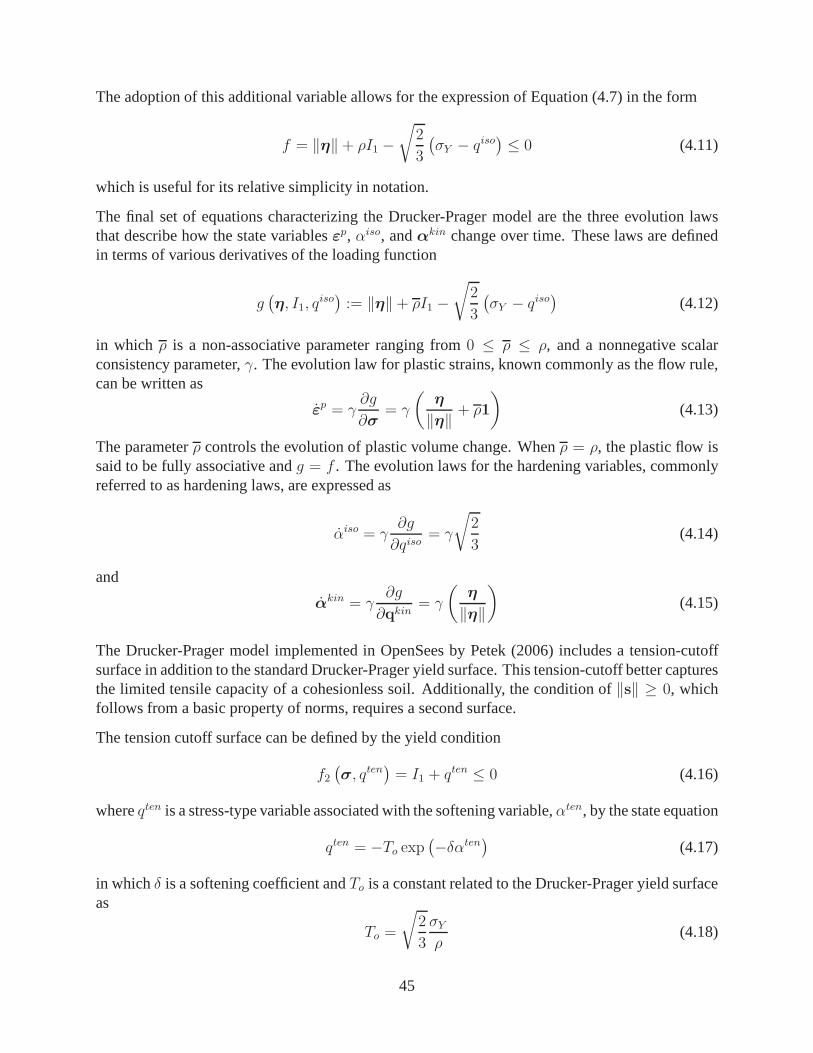
The adoption of this additional variable allows for the expression of Equation (4.7) in the form

f = ‖η‖+ ρI1 −√

2

3

(

σY − qiso)

≤ 0 (4.11)

which is useful for its relative simplicity in notation.

The final set of equations characterizing the Drucker-Prager model are the three evolution lawsthat describe how the state variablesεp, αiso, andαkin change over time. These laws are definedin terms of various derivatives of the loading function

g(

η, I1, qiso)

:= ‖η‖+ ρI1 −√

2

3

(

σY − qiso)

(4.12)

in which ρ is a non-associative parameter ranging from0 ≤ ρ ≤ ρ, and a nonnegative scalarconsistency parameter,γ. The evolution law for plastic strains, known commonly as the flow rule,can be written as

ε̇p = γ∂g

∂σ= γ

(

η

‖η‖ + ρ1

)

(4.13)

The parameterρ controls the evolution of plastic volume change. Whenρ = ρ, the plastic flow issaid to be fully associative andg = f . The evolution laws for the hardening variables, commonlyreferred to as hardening laws, are expressed as

α̇iso = γ∂g

∂qiso= γ

√

2

3(4.14)

and

α̇kin = γ∂g

∂qkin= γ

(

η

‖η‖

)

(4.15)

The Drucker-Prager model implemented in OpenSees by Petek (2006) includes a tension-cutoffsurface in addition to the standard Drucker-Prager yield surface. This tension-cutoff better capturesthe limited tensile capacity of a cohesionless soil. Additionally, the condition of‖s‖ ≥ 0, whichfollows from a basic property of norms, requires a second surface.

The tension cutoff surface can be defined by the yield condition

f2(

σ, qten)

= I1 + qten ≤ 0 (4.16)

whereqten is a stress-type variable associated with the softening variable,αten, by the state equation

qten = −To exp(

−δαten)

(4.17)

in whichδ is a softening coefficient andTo is a constant related to the Drucker-Prager yield surfaceas

To =

√

2

3

σYρ

(4.18)

45

The flow rule of Equation (4.13) is extended for the tension cutoff surface as

ε̇p = γ1∂g1∂σ

+ γ2∂f2∂σ

= γ1

(

η

‖η‖ + ρ1

)

+ γ21 (4.19)

and the softening law is formulated as

α̇ten = γ2∂f2∂qten

= γ2 (4.20)

4.4.2 Determination of Material Parameters

The material constants defining the Drucker-Prager constitutive model are selected such that thereis consistency with the elastic soil elements, as well as a degree of realism in the magnitudes usedfor each soil layer. To this end, the elastic constants of bulk and shear moduli defined for thelinear elastic soil models are used in the elastoplastic models. To create a more realistic pressure-dependent elastic stiffness in the elastoplastic model, the elastic parameters are modified to includethe ability to update the bulk modulus according to the relation

κ = κ0

√

1 +|σm||σref |

(4.21)

in which κ0 is the reference bulk modulus listed in Table 4.2,σm = I1/3 is the mean stress ineach element, andσref is a reference pressure taken to be equal to atmospheric pressure (101 kPa).A similar relation is used to update the shear modulus in the model, in whichG0 is the referenceshear modulus listed in Table 4.2.

In order to obtain sensible values for the Drucker-Prager material constantsρ andσY , the followingcorrelations have been made with the somewhat more common, and measurable, Mohr-Coulombmaterial constants of cohesion,c, and friction angle,φ, after the discussion detailed in Chen andSaleeb (1994) as follows:

ρ =2√2 sin φ√

3 (3− sin φ)(4.22)

σY =6c cosφ√

2 (3− sinφ)(4.23)

Assuming a small amount of cohesion for numerical stability, c = 3.56 kPa, and internal frictionangles ofφ = 36◦ in the unliquefied layers andφ = 0◦ in the liquefied layer, the Drucker-Pragermaterial constants are computed for each layer using Equations (4.22) and (4.23). These valuesare summarized in Table 4.2. With respect to associative andnon-associative plastic flow, severalcombinations are explored. Models are run with the non-associative parameterρ set equal to bothρ, creating fully associative flow, and zero, creating isochoric non-associative flow. Additionally,based on the assumptions of drained conditions and a medium initial density for the unliquefiedlayers, an intermediate case whereρ = 0.150 is used. This is done so that there will be somedilation of the soil, but not quite as much as would occur for the case withρ = ρ.

46

Table 4.2 Material input parameters used in Drucker-Pragersoil constitutive model.

Soil Layer κ0 (kPa) G0 (kPa) φ (◦) σY (kPa) ρ γ (kN/m3)

Unliquefied 27777.8 9260 36 5.00 0.398 17Liquefied 27777.8 842 0 4.97 0.000 17

It is interesting to note that when settingφ = 0◦, resulting inρ = 0, the Drucker-Prager yieldcondition of Equation (4.7) reduces to the von Mises yield criterion. In effect, the elastoplasticlateral spreading model is constructed by considering the unliquefied layers to be Drucker-Pragermaterials and the liquefied middle layer as a low shear stiffness von Mises material. To provide adegree of simplicity in the model, the linear isotropic hardening and tension softening parametersare set to zero in the lateral spreading simulations.

4.5 VALIDATION OF SOIL MODELS

As with all of the other aspects of this research, it is important to validate the elastoplastic soil mod-els through simple tests before installing them into a larger model. The Drucker-Prager soil modelis evaluated through a series simulated geotechnical testswith a single element of elastoplasticsoil. The chosen tests are all commonly performed to evaluate the mechanical characteristics ofsoil samples, and allow for validation that the OpenSees implementation of the Drucker-Pragermodel is performing as expected. The selected geotechnicaltests are:

1. Confined compression (CC) test

2. Conventional triaxial compression (CTC) test

3. Simple shear (SS) test

4. Hydrostatic extension (HE) test.

With the exception of the hydrostatic extension test, all ofthe simple, single element, tests startfrom an initial hydrostatic stress state,σ1 = σ2 = σ3 = −po, wherepo is an initial confiningpressure. Each test is conducted for various initial confining pressures both with and without theinclusion of linear isotropic hardening. Unless otherwiseindicated, the material parameters usedin each test are those listed in Table 4.2.

When dealing with 3D stress states, plots of the various invariants of the stress and strain tensorsare often the most effective means for visualizing the behavior of a particular material. If chosencarefully, such plots can display data in a more meaningful manner than traditional stress-strainplots. For each material test, four plots are chosen with theintent of fully characterizing the stress-strain response of the Drucker-Prager soil element. The chosen invariant axes include the norm ofthe deviatoric stress tensor,‖s‖, the first invariant of the stress tensor,I1 = trσ, the norm of thedeviatoric strain tensor,‖e‖, the trace of the strain tensor,tr(ε), and the mean stress,I1/3.

47

(a) (b)x

y

x

y

zz

Figure 4.2 Schematic depiction of the simulated CC test. (a)Hydrostatic compressionphase; (b) Confined compression phase.

4.5.1 Confined Compression Test

In a CC test the soil element is first brought to an initial state of hydrostatic stress. While holdingthe displacements fixed in the first and second principal stress directions, the displacement in thethird principal direction is increased, creating an increase in the compressive stress in that direction.To achieve this in the context of the single element model, anentirely strain-controlled approachis adopted. The approach used to model this test is depicted schematically in Figure 4.2.

As with the models in all of the soil tests, this model considers the soil element to be a unit cube.The nodes in thex - y, y - z, andz - x planes are held fixed with respect to displacements normal totheir faces. The nodes on the element faces opposite the fixedfaces are moved inwards by equalincrements to create the hydrostatic stress state. After the desired hydrostatic stress state has beenreached, the nodes on the positivex- andy-faces are held fixed againstx- andy-direction displace-ments, respectively, while the nodes on the positivez-face of the element are moved downwards,see Figure 4.2(b). The stresses acting in thex- andy-directions do not stay constant, instead, thestrains in those directions are held constant.

The stress path for the CC test is shown on the meridian plane (I1 − ‖s‖ axes) in Figure 4.3 forthree values of initial confining pressure (p0 = 10, p0 = 20, andp0 = 40 kPa). As expected, thenormal stress increases along theI1 axis during the hydrostatic loading phase, and then deviatoricstresses begin to develop during the confined compression phase. For the particular loading ratioused in the CC test, the soil element remains in the elastic range, never reaching the yield state, anevent that would be evident by the stress path intersecting the line of the failure surface. Becausethe element remains entirely elastic during this test, no strain hardening cases are considered.

The material-response summary presented Figure 4.4 shows the stress-strain behavior of the soilelement during the CC test on a series of four axes. Since the material remains entirely elasticduring this test, the slopes of the curves in all four plots remain constant. This verifies both theinitial expectations for this test as well as the stress pathshown in Figure 4.3.

48

−900 −800 −700 −600 −500 −400 −300 −200 −100 00

50

100

150

200

250

300

350

400

450

tr(σ) [kPa]

||s||

[kP

a]

failure surfacep

o = 10 kPa

po = 20 kPa

po = 40 kPa

Figure 4.3 Stress paths for CC test.

−0.01 −0.005 00

50

100

tr(ε)

||s||

[kP

a]

0 2 4 6 8x 10

−3

0

50

100

||e||

||s||

[kP

a]

−0.01 −0.005 0−300

−200

−100

0

tr(ε)

(1/3

)tr(

σ) [k

Pa]

0 2 4 6 8x 10

−3

−300

−200

−100

0

||e||

(1/3

)tr(

σ) [k

Pa]

po = 10 kPa

po = 20 kPa

po = 40 kPa

Figure 4.4 Stress-strain responses of Drucker-Prager soilelement subjected to CC teststress path.

49

x

y

x

y

z z

(a) (b)

Figure 4.5 Schematic depiction of the CTC test as performed in OpenSees. (a) Hydrostaticcompression phase; (b) Application of deviator stress.

4.5.2 Conventional Triaxial Compression Test

The CTC test is one of the most widely used test in soil mechanics. In this test, after the initialhydrostatic loading phase, two of the principal stresses are kept constant (i.e.,σ1 = σ2 = −po),while the third principal stress,σ3 is increased. This test differs from the confined compressiontest in that the first and second principal stresses do not change from their initial value at the theend of the hydrostatic phase, whereas the first and second principal stresses in the CC test increasein proportion to the applied stress increase in the third principal direction.

The CTC test is achieved in a single element model as depictedin Figure 4.5. This test uses mixedstress and strain control as opposed to the pure strain control of the CC test, however, the geometricboundary conditions are the same as those in the CC test model. The hydrostatic stresses areapplied under stress control, by applying compressive loads on the free degrees of freedom. Oncethe desired hydrostatic state is achieved, the loads on the positivex- andy-faces are held fixed forthe duration of the test, ensuring that the principal stresses in two directions remain constant, whilethe nodes on the positivez-face of the element are moved downwards under strain control to createthe increase in the third principal stress. The nodes on the non-fixed faces of the element are leftfree to displace outward during this process.

Verification that the material model behaves in a predictable manner during this test can be obtainedthrough a comparison of the predicted slope of the stress path resulting from the CTC test with thedata returned from OpenSees. It can be shown that the slope ofthe CTC test stress path on ameridian (I1−‖s‖) plane, is equal to

√

2/3. A line with this slope is plotted against the stress pathreturned from OpenSees for thep0 = 10 kPa case. As shown in Figure 4.6, the single element testslope is identical to the theoretical slope, thus providingfurther validation that the Drucker-Pragermaterial model has been successfully implemented into OpenSees.

The simulated CTC stress paths for a soil element with no strain hardening are shown in Figure 4.7for three values of initial confining pressure,p0. A corresponding plot is shown in Figure 4.8for a soil element including linear isotropic strain hardening. For the strain hardening cases, the

50

−70 −60 −50 −40 −30 −20 −10 00

5

10

15

20

25

30

35

40

45

50

tr(σ) [kPa]

||s||

[kP

a]

failure surfaceTheoretical Stress PathOpenSees Stress Path

Figure 4.6 Comparison of simulated and theoretical CTC teststress paths.

hardening parameterK is set to100, 000 kPa to enhance visualization. The CTC test brings theelement to failure for all cases. For the three cases withoutstrain hardening, once the deviatoricstress has increased to the point where the stress path intersects the failure surface, the materialyields and the stresses no longer increase with increasing strain. This behavior is consistent withthe expectations for a perfectly plastic material.

When linear isotropic hardening is included, the model exhibits behavior that is somewhat altered.Instead of displaying perfectly plastic behavior, the soilelement hardens with increasing strain,allowing for the stresses to increase beyond the initial limiting values for the perfectly plastic cases.The inclusion of strain hardening effectively acts to expand the failure surface with increasingplastic strain. Again, the Drucker-Prager soil element behaves as expected, providing assurancethat the OpenSees implementation is correct.

The stress and strain invariant plots of Figures 4.9 and 4.10provide a more complete look at theplastic behavior of the soil element during the CTC test. Theperfectly plastic behavior of the modelfor the cases without strain hardening is even more evident in Figure 4.9 than in Figure 4.7. Afterthe elastic portion of the loading, the slopes of the curves all go to zero, indicating increases in shearand normal strain with no corresponding increases in shear or normal stress. For the cases withstrain hardening, there is a change in slope at the end of the elastic range, however, here the slopesdo not go to zero, instead they change according the the amount of strain hardening considered.The behavior displayed in these two figures validates that the OpenSees implementation of theDrucker-Prager model displays the intended post-yield behavior when the soil is brought to yieldby an increase in normal stress.

51

−350 −300 −250 −200 −150 −100 −50 0 50−50

0

50

100

150

200

tr(σ) [kPa]

||s||

[kP

a]

failure surfacep

o = 10 kPa

po = 20 kPa

po = 40 kPa

Figure 4.7 Stress paths for CTC test in the perfectly plasticcase (no strain hardening).

−350 −300 −250 −200 −150 −100 −50 0 50−50

0

50

100

150

200

tr(σ) [kPa]

||s||

[kP

a]

failure surfacep

o = 10 kPa

po = 20 kPa

po = 40 kPa

Figure 4.8 Stress paths for CTC test the linear isotropic strain hardening case.

52

0 5 10x 10

−3

0

20

40

60

80

100

120

tr(ε)

||s||

[kP

a]0 0.005 0.01 0.015 0.02

0

20

40

60

80

100

120

||e||

||s||

[kP

a]

0 5 10x 10

−3

−100

−80

−60

−40

−20

0

tr(ε)

(1/3

)tr(

σ) [k

Pa]

0 0.005 0.01 0.015 0.02−100

−80

−60

−40

−20

0

||e||(1

/3)t

r(σ)

[kP

a]

po = 10 kPa

po = 20 kPa

po = 40 kPa

Figure 4.9 Stress-strain responses of Drucker-Prager soilelement subjected to a CTC stresspath for the perfectly plastic case (no strain hardening).

−3 −2 −1 0x 10

−3

0

50

100

150

200

tr(ε)

||s||

[kP

a]

0 0.005 0.010

50

100

150

200

||e||

||s||

[kP

a]

−3 −2 −1 0x 10

−3

−120

−100

−80

−60

−40

−20

0

tr(ε)

(1/3

)tr(

σ) [k

Pa]

0 0.005 0.01−120

−100

−80

−60

−40

−20

0

||e||

(1/3

)tr(

σ) [k

Pa]

po = 10 kPa

po = 20 kPa

po = 40 kPa

Figure 4.10 Stress-strain responses of Drucker-Prager soil element subjected to a CTCstress path for the linear isotropic strain hardening case.

53

(a) (b)

y

x x

y

zz

Figure 4.11 Schematic depiction of the SS test as performed in OpenSees. (a) Hydrostaticcompression phase; (b) Simple shear phase.

4.5.3 Simple Shear Test

In the SS test, the soil element is brought to failure in pure shear, i.e.,∆I1 = 0. The OpenSees im-plementation of the SS stress path is conducted entirely under strain control. Figure 4.11 providesa visual representation of the single element SS test as analyzed in OpenSees. The initial hydro-static state is induced in an identical manner to the previously described CC test. From this initialhydrostatic state, the nodes at the base of the element are held fixed while the upper nodes aredisplaced in the negativey-direction by equal increments. During this test, the uppernodes are notdisplaced in thex- or z-directions, resulting in an isochoric deformation. This type of deformationresults in the desired state of pure shear stress (small strain only).

The SS test is run for three values of initial confining pressure, both with and without the inclusionof linear isotropic strain hardening. Figure 4.12 shows thestress paths for the three confiningpressures on the meridian plane for the perfectly plastic cases; and Figure 4.13 shows the stress-strain behavior during this test. In the elastic range, the element only experiences an increasein deviatoric stress, the expected behavior. Once the soil element yields, the mean normal stressdecreases (increased compression), and the deviatoric stress continues to increase with increasingdeviatoric strain. However, there is no change in the total volumetric strain. The initial drop involumetric strain,tr ε, indicated in Figure 4.13 corresponds to the hydrostatic loading phase.

Figures 4.14 and 4.15 show the stress paths and the stress-strain behavior, respectively, for a soilelement with linear isotropic strain hardening. A hardening coefficient ofK = 100, 000 kPa isselected for for enhanced visualization. For these cases, the elastic behavior is unchanged; thestress path lies in the deviatoric plane from the initial hydrostatic state up until the initial yieldpoint. Subsequent yielding under the inclusion of strain hardening allows for greater increases indeviatoric stress during the continued application of increasing deviatoric strains.

The results of the single element simple shear tests providefurther validation that the Drucker-Prager material model reproduces the expected behaviors when subject to known stress/strainpaths. When implemented in an element subject to pure shear,the material model is able to produceconsistent results for all of the investigated cases.

54

−200 −150 −100 −50 0 50−50

0

50

100

tr(σ) [kPa]

||s||

[kP

a]

failure surfacep

o = 10 kPa

po = 20 kPa

po = 40 kPa

Figure 4.12 Stress paths for SS test in the perfectly plasticcase (no strain hardening).

−1.5 −1 −0.5 0x 10

−3

0

20

40

60

80

100

tr(ε)

||s||

[kP

a]

0 2 4 6x 10

−3

0

20

40

60

80

100

||e||

||s||

[kP

a]

−1.5 −1 −0.5 0x 10

−3

−60

−40

−20

0

tr(ε)

(1/3

)tr(

σ) [k

Pa]

0 2 4 6x 10

−3

−60

−40

−20

0

||e||

(1/3

)tr(

σ) [k

Pa]

po = 10 kPa

po = 20 kPa

po = 40 kPa

Figure 4.13 Stress-strain responses of Drucker-Prager soil element subjected to a SS teststress path for the perfectly plastic case (no strain hardening).

55

−200 −150 −100 −50 0 50−50

0

50

100

tr(σ) [kPa]

||s||

[kP

a]

failure surfacep

o = 10 kPa

po = 20 kPa

po = 40 kPa

Figure 4.14 Stress paths for SS test in the linear isotropic strain hardening case.

−1.5 −1 −0.5 0x 10

−3

0

20

40

60

80

100

tr(ε)

||s||

[kP

a]

0 2 4 6x 10

−3

0

20

40

60

80

100

||e||

||s||

[kP

a]

−1.5 −1 −0.5 0x 10

−3

−60

−40

−20

0

tr(ε)

(1/3

)tr(

σ) [k

Pa]

0 2 4 6x 10

−3

−60

−40

−20

0

||e||

(1/3

)tr(

σ) [k

Pa]

po = 10 kPa

po = 20 kPa

po = 40 kPa

Figure 4.15 Stress-strain responses of Drucker-Prager soil element subjected to a SS teststress path for the linear isotropic strain hardening case.

56

x

y

z

Figure 4.16 Schematic depiction of the HE test as performed in OpenSees.

4.5.4 Hydrostatic Extension Test

The final single element test performed in pursuit of validating the OpenSees implementation ofthe Drucker-Prager material model is a hydrostatic extension (HE) test. In this test, the soil elementis subject to equally increasing principal stresses until failure is achieved. The resulting stress pathfollows the hydrostatic axis in the tensile direction, eventually reaching the tip of the cone depictedin Figure 4.1.

To achieve the HE test in a single element model, the procedure is essentially the opposite ofthe hydrostatic compression phases of the prior tests. Fromthe same base model and boundaryconditions, the free nodes are displaced outward in equal increments as represented schematicallyin Figure 4.16. The HE test is performed both to test the tensile behavior of the model and toevaluate the effectiveness of the tension-cutoff implementation.

Due to the nature of this test, multiple confining pressures were not included in the results. How-ever, the HE test is conducted for three values of the tensionsoftening coefficient,δ. As shownin Figure 4.17, the intended stress path is returned by the model. Providing assurance that theDrucker-Prager material model can handle tensile stressesas well as compressive stresses. Thestress and strain invariant plots of Figure 4.18 verify thatthe element develops no deviatoric strainsnor stresses during the single element HE test. As is expected, only normal stresses and strains areexperienced by the soil element.

The effect of changes in the the magnitude ofδ is evident in the lower left plot of Figure 4.18.When δ = 0, the element displays perfectly plastic behavior after thetensile limit is reached,indicating that no softening occurs. The degree of softening increases with increasing values ofδ, just as intended by the inclusion of the tension softening surface in the material model. Allof the behavior displayed by the Drucker-Prager soil element in the HE test is consistent withexpectations, thus providing further verification as to thecorrect implementation of the materialmodel in OpenSees.

57

−2 0 2 4 6 8 10 12−2

−1

0

1

2

3

4

5

6

tr(σ) [kPa]

||s||

[kP

a]

failure surfaceδ

2 = 0

δ2 = 5000

δ2 = 10000

Figure 4.17 Stress paths for HE test, on the meridian plane for three values of the tensionsoftening parameter,δ.

0 1 2 3 4x 10

−4

0

1

2

3

4x 10

tr(ε)

||s||

[kP

a]

0 1 2 3 4x 10

−4

0

1

2

3

4x 10

||e||

||s||

[kP

a]

0 1 2 3 4x 10

−4

0

1

2

3

tr(ε)

(1/3

)tr(

σ) [k

Pa]

0 1 2 3 4x 10

−4

0

1

2

3

||e||

(1/3

)tr(

σ) [k

Pa]

δ2 = 0

δ2 = 5000

δ2 = 10000

Figure 4.18 Stress-strain response of Drucker-Prager soilelement subjected to a HE teststress path for three values of tension softening parameter, δ.

58

3 m

2 m

Figure 4.19 A representation of the load case modeled by the multi-element plane straintest for the Drucker-Prager material model.

4.5.5 Multi-Element Plane Strain Test

In the mechanical behavior tests described in Sections 4.5.1 through 4.5.4, the OpenSees imple-mentation of the Drucker-Prager material model is tested with the use of a single element. Toassess the model in a somewhat broader context, a multi-element plane strain test is conducted. Aschematic of this test is shown in Figure 4.19. In this test, adistributed load is applied to a portionof the upper surface of a wall of soil material. The base of themodel is held fixed against verti-cal displacements, and the large planar surfaces of the model are held fixed against out-of-planedisplacements to create plane strain conditions. The symmetry shown in Figure 4.19 is applied byfixing displacements in the horizontal direction. The purpose of this plane strain test is to evaluatethe behavior of the Drucker-Prager material model in the context of a multi-element model.

The mesh for the plane strain test is3 m wide,3 m tall, and1 m thick. The soil elements are definedwith the unliquefied layer material parameters summarized in Table 4.2. A distributed load isapplied over a1 m square. This load is increased linearly until the two nodesin the symmetry planehave undergone a5 mm downward displacement. The deformed shape of the mesh, magnified bya factor of ten, is shown in Figure 4.20 along with the distribution of the vertical stress component,σyy. As shown, the model is reacting in a manner consistent with initial expectations. Compressivestresses develop in the left hand portion of the model (the area beneath the load), while tensilestresses are generated in the right hand portion as those soil elements expand. Though the presentedresults are only for a twenty-four element square mesh, thissame test was conducted with differingnumbers of elements. In all cases the model displays predictable behavior as well as a quadraticrate of asymptotic convergence, further validating the OpenSees implementation of the Drucker-Prager material model.

To further illustrate and verify the abilities of the Drucker-Prager material model, the stress pathsfor several Gauss points along the top row of the mesh are plotted on the meridian plane in Fig-ure 4.21. As shown, several elements are brought to yield in both tension and compression, whileothers remain in the elastic range during the test. Figure 4.21 provides further validation thatthe Drucker-Prager soil elements can be successfully implemented in a multi-element model, onewhich causes the elements to undergo a variety of stress paths.

59

Figure 4.20 The deformed mesh for the plane strain test with the distribution of verticalstress in the soil elements (magnification factor = 10).

−100 −80 −60 −40 −20 0−5

0

5

10

15

20

25

30

35

tr(σ) [kPa]

||s||

[kP

a]

failure surfaceelement 553element 555element 558element 559element 561element 562element 566element 571element 576

Figure 4.21 Stress paths for a selection of Gauss points along the top row of the plane strainmodel.

60

5 Three-Dimensional Finite Element Analysis

5.1 INTRODUCTION

Piles embedded in laterally spreading cohesionless soils must be able to withstand large bendingdemands. The magnitude and location of the largest shear andmoment demands are dependentupon many factors. Among these factors are the size and stiffness of the pile, the strength of thesurrounding soil, the boundary and support conditions of the pile, the amount of lateral displace-ment that occurs, and the depth of the liquefied layer.

Single piles in laterally spreading soil systems are analyzed by means of a 3D FE model (seeChapter 2). This model includes beam elements for the piles,brick elements for the soil, andbeam-solid contact elements to define the interaction between the pile and the surrounding soil.Two separate pile head support conditions are considered inthese simulations: (1) a fixed-headcondition and, (2) a free-head condition. The fixed-head condition restricts the rotation of the pilehead and is the most representative of an actual pile application, while the free-head cases allowthe pile head to rotate freely and provide a means of comparison.

In all of the considered cases, the piles are subject to the imposed displacement profile discussedin Section 2.3 having a magnitude of one pile radius in the upper soil layer. This distance issufficient to cause inelastic behavior in the elastoplasticpile and soil models, while remainingsmall enough to facilitate relatively short run-times in OpenSees. Run-time per case ranges fromapproximately four hours in linear elastic cases to26 hours in elastoplastic cases, and varies forthe three pile models. For all cases the thickness of the liquefied layer is set at one pile diameter.The dimensional scheme discussed in Section 2.2 is utilized, with a liquefied layer located ten pilediameters below the ground surface.

The behavior of a single pile in a laterally spreading soil system is evaluated through comparisonsbetween the data returned from each of 24 cases run with various combinations of piles, soil, andpile support conditions. The models are evaluated via the bending behavior of the piles, the stressesthat develop in the soil, and the soil-pile interface forcesdeveloping in the contact elements, amongother factors. The individual results of each modeling approach are examined and compared inorder to provide further insight into the lateral spreadingproblem.

61

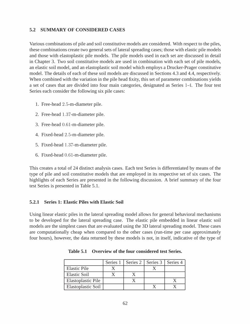
5.2 SUMMARY OF CONSIDERED CASES

Various combinations of pile and soil constitutive models are considered. With respect to the piles,these combinations create two general sets of lateral spreading cases; those with elastic pile modelsand those with elastoplastic pile models. The pile models used in each set are discussed in detailin Chapter 3. Two soil constitutive models are used in combination with each set of pile models,an elastic soil model, and an elastoplastic soil model whichemploys a Drucker-Prager constitutivemodel. The details of each of these soil models are discussedin Sections 4.3 and 4.4, respectively.When combined with the variation in the pile head fixity, thisset of parameter combinations yieldsa set of cases that are divided into four main categories, designated as Series1-4. The four testSeries each consider the following six pile cases:

1. Free-head2.5-m-diameter pile.



4. Fixed-head2.5-m-diameter pile.



This creates a total of 24 distinct analysis cases. Each testSeries is differentiated by means of thetype of pile and soil constitutive models that are employed in its respective set of six cases. Thehighlights of each Series are presented in the following discussion. A brief summary of the fourtest Series is presented in Table 5.1.

5.2.1 Series 1: Elastic Piles with Elastic Soil

Using linear elastic piles in the lateral spreading model allows for general behavioral mechanismsto be developed for the lateral spreading case. The elastic pile embedded in linear elastic soilmodels are the simplest cases that are evaluated using the 3Dlateral spreading model. These casesare computationally cheap when compared to the other cases (run-time per case approximatelyfour hours), however, the data returned by these models is not, in itself, indicative of the type of

Table 5.1 Overview of the four considered test Series.

Series 1 Series 2 Series 3 Series 4Elastic Pile X XElastic Soil X XElastoplastic Pile X XElastoplastic Soil X X

62

behavior that would occur in an actual lateral spreading event. Instead of offering direct insightsinto pile behavior, the fully elastic cases provide a benchmark for comparison and evaluation ofmore computationally intensive models.

5.2.2 Series 2: Elastoplastic Piles with Elastic Soil

The use of elastoplastic pile models allows for the examination of the interaction between the soiland the pile during a lateral spreading event in a more realistic fashion than that which is returnedby elastic pile models. When using elastoplastic piles, thepiles are able to yield and developplastic hinges under the influence of the imposed displacement profile. This changes the way inwhich the soil and pile interact in the model, often in dramatic fashion. This Series is considered asan intermediate set of cases through which comparisons can be drawn between the entirely linearelastic cases (Series1) and the entirely elastoplastic series of cases (Series4). Additionally, thisseries allows for the effects of plastic behavior in the piles to be examined in an isolated fashion.

5.2.3 Series 3: Elastic Piles with Elastoplastic Soil

These six cases offer a direct means of evaluation for the effects of yielding in the soil on thebehavior of the pile in the lateral spreading case. Leaving the pile elastic creates a situation inwhich the only differences between these cases and the entirely elastic cases must be due to theplastic behavior of the soil, allowing any mechanisms to be pinpointed. Additionally, the elasticpile in elastoplastic soil series allows for the extractionof p –y curves at various depths within thesoil system, providing a means of comparison for the resultsof the 3D lateral spreading modelwith other, more commonly used models for the lateral analysis of piles. Thep –y curves aredetermined from the resulting contact forces applied to each pile node and the displacement of thepile relative to the soil at each of these positions. Furtherdiscussion on this process can be foundin Chapter 6.

5.2.4 Series 4: Elastoplastic Piles in Elastoplastic Soil

The fully elastoplastic cases offer the most realistic glimpse into the behavior of the lateral spread-ing problem, though at the highest computational cost (run-times approximately24 to 26 hours).This set of cases enables observations to be made into the behaviors that develop when both thepiles and the soil yield and display plastic behavior. Additionally, it is of interest to evaluate ifthe results found in the fully elastoplastic series can be successfully reproduced by using a BNWFanalysis with elastoplastic pile models and thep –y curves computed from the Series 3 model.

63

Figure 5.1 Deformed shape and distribution of lateral stress for the Series1 free-head casewith a 0.61-m-diameter pile. Stresses are given in kPa.

5.3 GENERAL BEHAVIOR OF PILES IN LATERALLY SPREADING SOIL

In all of the cases, the interaction between the soil and the pile, governed by their respectivematerial properties, defines the resulting behavior of the system. General patterns of behavior areobserved through consideration of several comparative measures. These results are deemed mostindicative of the pile behavior as a whole, and include the magnitudes of the maximum momentand shear force demands in the pile, and the locations of these extreme values. Also of interest arethe evolution of the extreme moments in in the pile, and the way in which the lateral spreading soildeformation profile manifests itself as a load on the pile.

As the upper layer of soil begins to displace laterally with respect to the immobile lower layer, theentire pile provides resistance to this motion as the upper portion is pushed along with the flowof soil. This behavior is illustrated in Figure 5.1, which shows the the distribution of horizontalnormal stress (in the direction of motion) in the soil elements, as well as the deformed shape of thesystem, for the Series1 free-head case with a0.61-m-diameter pile.

The entirely linear elastic case is selected for Figure 5.1 to illustrate the lateral stress distributionin the soil because it allows truly large stresses to develop. The locations of the largest tensileand compressive lateral stress in the elastic soil elementsidentify where initial yielding is likely tooccur in both the elastoplastic soil models and in an actual soil system. If the elements are assignedelastoplastic behavior, the yielding that may occur would likely obscure the marked differences instresses that are able to develop in the linear elastic case,making it difficult to differentiate betweenthe stresses in adjacent locations.

From the lateral stresses developed in the vicinity of the pile, it can be clearly seen that the imposeddisplacement profile puts the pile in bending. In the lower solid layer, the distribution of compres-

64

sive stresses shows that the pile pushes back into the soil atits base while it is pushed into the soilat the interface with the liquefied soil layer. The opposite is observed in the upper soil layer, wherethe pile resists the ground motion at the interface with the liquefied layer and is pushed into thesoil at the pile head. Additionally, at each location of large compressive stress on the leading andtrailing faces of the pile, there is a corresponding zone of tensile stress in the soil. These tensileregions signify where the soil elements are being pulled apart by either the passive or active pas-sage of the pile through the soil. While the results of Figure5.1 are for a0.61-m-diameter pile,this same pattern of lateral stress is present in all of the lateral spreading models.

In addition to the lateral stress near the pile, it is also of interest to observe the distribution oflateral stresses in the remainder of the soil system. The lateral stresses in the liquefied layer remainrelatively small during the simulated lateral spreading event, however, the imposed ground motioncauses large compressive and tensile stresses to develop inthe solid soil layers at the boundaries ofthe model. These zones of increased stress are higher near the symmetry plane. Though these dis-tributions are most certainly at least partially due to the boundary and loading conditions imposedupon the model, these results suggest that the pile is able toinfluence a far wider area than just itsimmediate vicinity during a lateral spreading event.

Figure 5.2 shows a series of plots that detail exactly how thelateral spreading ground motionaffects the embedded pile. This figure presents results obtained from the same0.61-m-pile caseas the lateral stress distribution shown in Figure 5.1, the entirely linear elastic, free pile head case.This series of summary plots illustrates the general pattern of shear force and bending momentdemands that develop in a pile during a lateral spreading event, as well as the deflected shape ofthe pile. All of the piles display distributions of bending demands that are similar in form to thegeneral shapes presented here.

The maximum shear force demand occurs at the center of the liquefied layer, depicted as the shadedregion in Figure 5.2, where the differential motions of the two solid layers are felt most stronglyby the pile, and minimal resistance is provided by the liquefied soil. It can be expected that in anylateral spreading event, the largest shear force demand will occur at, or very near, this location.There are also extreme values of shear in each of the two solidlayers, located approximately two-thirds of the total layer thickness away from the interface with the liquefied layer. The extremeshear demand in the lower layer is greater due to the increasein confining stress with depth.

The locations of minimum moment occur at the center of the liquefied layer, where there is zeromoment, and due to the boundary condition of this model, at each end of the pile, where themoment is also zero. The extreme moments in the pile correspond to the locations of zero shearforce, with one maximum in each of the unliquefied soil layers. The absolute maximum momentoccurs in the lower solid layer. As with the extreme shear force demand in that layer, the extrememoment demand here is larger than the extreme value in the upper layer due to the increasedoverburden pressure with depth. The locations of the extreme moments in each layer tend tostay relatively constant in this entirely linear elastic model. The distance between these locationsdefines an effective length,Leff , for the pile, as shown schematically in Figure 5.3. The effectivelength is a parameter signifying, in part, the influence of the liquefied layer on the pile. Theeffective length is a convenient parameter to use in simplified analyses of the lateral spreadingproblem, as well as a useful parameter for comparing the results for the various pile sizes.

65

Applied Load (kN/m)

Hei

ght a

bove

bas

e (

m)

Load distribution for 0.6096 m pile

−1500 −1000 −500 0 500 1000 15000

2

4

6

8

10

12

Deflection (m)

Hei

ght a

bove

bas

e (

m)

Deflected shape of 0.6096 m pile

0 0.05 0.1 0.15 0.2 0.25 0.30

2

4

6

8

10

12

pseudo time

Hei

ght a

bove

bas

e (

m)

Location of extreme moments for 0.6096 m pile

12 14 16 18 200

2

4

6

8

10

12 position of maxM in top layerposition of maxM in bottom layerL

effective

12 14 16 18 20

500

1000

1500

2000

pseudo time

Mo

me

nt M

(k

Nm

)

Extreme moments for 0.6096 m pile

abs(max M) in top layerabs(max M) in bottom layer

Moment (kNm)

Hei

ght a

bove

bas

e (

m)

Moment distribution for 0.6096 m pile

−2000−1500−1000 −500 0 500 1000 15000

2

4

6

8

10

12

Shear force (kN)

Hei

ght a

bove

bas

e (

m)

Shear force distribution for 0.6096 m pile

−2000 −1500 −1000 −500 0 5000

2

4

6

8

10

12

Shear force distribution

Load distributionEvolution of deflected shape

Evolution of extreme moments Location of extreme moments

Moment distribution

Figure 5.2 Pile summary plots for a 0.61-m-diameter pile. Series 1, free-head case. Theliquefied layer is the shaded region.

66

Leff

Figure 5.3 The effective length,Leff , is the distance between the extreme moments in eachsolid soil layer, as shown in this moment diagram.

In addition to the plots related to the deformation and bending demands in the pile, Figure 5.2 alsoshows the distribution of load imposed upon the pile by the lateral flow of the upper soil layer. Thisplot of the load distribution on the pile is determined from the slope of the shear diagram using thefamiliar relation

dV

dx= −w(x) (5.1)

in whichw(x) is the distributed load andV is the shear force. The plot of the load distributionprovides a insight into how the displacement of the surrounding soil manifests as load acting uponthe pile and corresponds well to the distribution of lateralstress in the soil, as shown in Figure 5.1.The magnitude and shape of this load profile varies from pile to pile and also shows a dependenceon the constitutive models used to represent the pile and thesoil, though the shape presented inFigure 5.2 is indicative of the general shape resulting fromeach case.

It is also observed that the liquefied layer of soil affects the behavior of the solid soil layers. Thedegree of this influence depends upon a few factors, including the stiffness of the pile and theconstitutive model used for the soil. Additionally, the degree of influence of the liquefied layer onthe soil near its boundaries is most significant in the vicinity of the pile, becoming less apparent asdistance from the pile increases. The cases with elastoplastic soils exhibited an increased amountof interaction between the unliquefied and liquefied soil layers, with the unliquefied layers beingpushed into the weaker liquefied layer. Figure 5.4 shows the pile pushing the unliquefied (dark)soil elements into the liquefied (light) layer for the Series4 case for a0.61-m-diameter pile. Themotion of the upper layer is to the right. As shown, this behavior occurs on either side of the pilein the areas in which the pile is cutting into the soil. In addition to the push-out observed on theleading edges of the pile, there is significant gapping taking place on the trailing edges of the pile,leading to the evident mesh distortion.

The behavior displayed in Figure 5.4 during the lateral spreading motion lessens the amount oflateral resistance that can be provided by the soil in the area surrounding the liquefied layer. Theunliquefied soil can be pushed into the adjacent weaker layermore easily than it can be pushed intothe adjacent solid soil elements or flow around the pile, effectively reducing the strength and stiff-ness of the unliquefied soil near the liquefied layer. This reduction in resistance can significantlyalter the behavior of the pile, causing increased curvaturedemands and increasing the potential for

67

Figure 5.4 Soil deformation pattern in the vicinity the pile for the Series4 case highlightingthe unliquefied soil elements pushing into the liquefied layer.

the formation of plastic hinges. Additionally, this reduction in soil strength results in a smallereffective length for the pile, which results in an increasedmoment and curvature demand on thepile and a corresponding increase in the potential for pile failure due to the lateral spreading event.

5.4 SUMMARY OF RESULTS FROM THREE-DIMENSIONAL LATERALSPREADING SIMULATIONS

A small parametric study consisting of 24 distinct cases is conducted using the 3D lateral spreadingmodel. There are three pile designs included in the study, each with elastic and elastoplasticconstitutive formulations. These piles are given two separate boundary conditions: a fixed pilehead condition and a free pile head condition. There are two soil constitutive models incorporatedinto the study, one linear elastic and the other an elastoplastic Drucker-Prager model. In all of thesimulations the liquefied layer is assigned a thickness of one pile diameter, this layer is centeredbetween two 10 pile diameter thick unliquefied soil layers; and the lateral displacement of theupper unliquefied layer with respect to the lower layer is onepile radius.

The results of all 24 lateral spreading cases are summarizedin Tables 5.2, 5.3, and 5.4 for the2.5-m, 1.37-m, and0.626-m piles, respectively. These tables list the maximum values of shear force,maxV , moment,maxM , curvature,maxφ, and displacement,maxU , for the pile, as well as theeffective length,Leff . The data in these tables is separated based upon the particular parametersand constitutive models used in each of four Series, as well as by the fixity of the pile head in eachsimulation. The specifics of each of the four Series are summarized in Table 5.1.

From the results presented in Tables 5.2, 5.3, and 5.4, a few behavioral trends are observed. Thestiffness of the pile, or more importantly the ratio of the pile stiffness to the lateral stiffness of the

68

Table 5.2 Summary of 3D lateral spreading analyses for the 2.5-m-diameter pile.

Pile-Soil Type maxV (kN) maxM (kNm) maxφ (m−1) maxU (m) Leff (m)

Series 1: Free 46100 235500 0.0012 1.47 17.62Series 2: Free 40600 186600 0.0021 1.43 16.19Series 3: Free 54000 300500 0.0015 1.57 16.14Series 4: Free 48800 227200 0.0036 1.51 15.11

Series 1: Fixed 53500 389500 0.0020 1.27 35.51Series 2: Fixed 42600 195500 0.0023 1.30 18.32Series 3: Fixed 63200 393500 0.0020 1.30 18.77Series 4: Fixed 50900 230100 0.0039 1.33 15.96









69

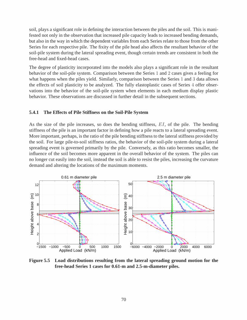
soil, plays a significant role in defining the interaction between the piles and the soil. This is mani-fested not only in the observation that increased pile capacity leads to increased bending demands,but also in the way in which the dependent variables from eachSeries relate to those from the otherSeries for each respective pile. The fixity of the pile head also affects the resultant behavior of thesoil-pile system during the lateral spreading event, though certain trends are consistent in both thefree-head and fixed-head cases.

The degree of plasticity incorporated into the models also plays a significant role in the resultantbehavior of the soil-pile system. Comparison between the Series1 and2 cases gives a feeling forwhat happens when the piles yield. Similarly, comparison between the Series1 and3 data allowsthe effects of soil plasticity to be analyzed. The fully elastoplastic cases of Series4 offer obser-vations into the behavior of the soil-pile system when elements in each medium display plasticbehavior. These observations are discussed in further detail in the subsequent sections.

5.4.1 The Effects of Pile Stiffness on the Soil-Pile System

As the size of the pile increases, so does the bending stiffness,EI, of the pile. The bendingstiffness of the pile is an important factor in defining how a pile reacts to a lateral spreading event.More important, perhaps, is the ratio of the pile bending stiffness to the lateral stiffness provided bythe soil. For large pile-to-soil stiffness ratios, the behavior of the soil-pile system during a lateralspreading event is governed primarily by the pile. Conversely, as this ratio becomes smaller, theinfluence of the soil becomes more apparent in the overall behavior of the system. The piles canno longer cut easily into the soil, instead the soil is able toresist the piles, increasing the curvaturedemand and altering the locations of the maximum moments.

Applied Load (kN/m)

Hei

ght a

bove

bas

e (

m)


−6000 −4000 −2000 0 2000 4000 60000

10

20

30

40

50

Applied Load (kN/m)

Hei

ght a

bove

bas

e (

m)


−1500 −1000 −500 0 500 1000 15000

2

4

6

8

10

12

0.61 m diameter pile 2.5 m diameter pile

Figure 5.5 Load distributions resulting from the lateral spreading ground motion for thefree-head Series 1 cases for 0.61-m and 2.5-m-diameter piles.

70

The load distribution plots of Figure 5.5, which show the loading applied to the pile by the imposedlateral spreading displacement for the Series1 free pile head cases for0.61-m and2.5-m-diameterpiles, typify the differences between small and large pile-to-soil stiffness ratios. It is important tonote that the load distributions shown in Figure 5.5 are the loads that are felt by the piles over theirrespective lengths. These loads are the result of both the soil pushing against the pile in the upperlayer and the pile pushing against the soil in the lower layer. If the pile-to-soil stiffness ratios foreach model were set to be equal, the resulting load distributions would be identical despite theincreased size of the larger pile.

For the0.61-m-diameter pile, which has a relatively small stiffness ratio, the magnitude of the loadapplied by the surrounding soil is much smaller than it is forthe2.5-m-diameter pile.

Deflection (m)

Hei

ght a

bove

bas

e (

m)


0 0.05 0.1 0.15 0.2 0.25 0.30

2

4

6

8

10

12

Deflection (m)

Hei

ght a

bove

bas

e (

m)


0 0.5 10

10

20

30

40

50

Deflection (m)

Hei

ght a

bove

bas

e (

m)


0 0.2 0.4 0.6 0.8 1 1.2 1.40

10

20

30

40

50

Deflection (m)

Hei

ght a

bove

bas

e (

m)


0 0.05 0.1 0.15 0.2 0.25 0.30

2

4

6

8

10

12

(a) (b)

(c) (d)

Figure 5.6 Deflected shapes of free-head piles for various cases. (a) Series 1, 0.61-m-diameter; (b) Series 1, 2.5-m-diameter; (c) Series 2, 0.61-m-diameter; (d) Series2, 2.5-m-diameter.

71

This indicates that the stiffer2.5-m-diameter pile is cutting further into the soil, activating moreresistance from the surrounding soil elements. This is confirmed by the displaced shapes for thesetwo piles shown in Figure 5.6. In the entirely linear elasticSeries1 case shown in Figure 5.6(b),the 2.5-m-diameter pile remains almost straight during the deformation due to its high stiffnessratio. The corresponding case for the0.61-m-diameter pile shown in Figure 5.6(a) displays visiblecurvature, indicating that the soil imposes larger curvature and bending demands on the pile withthe smaller pile-to-soil stiffness ratio.

The elastoplastic pile in elastic soil Series2 cases of Figures 5.6(c) and (d) accentuate this obser-vation. Even with elastoplastic pile elements creating thepotential for plastic hinge formation, thedisplaced shape of the stiffer pile remains essentially straight and is much further from the imposeddisplacement profile than the softer pile, providing verification that this trend is not isolated to theentirely elastic cases.

The effects of the pile-to-soil stiffness ratio can also be seen in the locations of the maximummoments for each of the piles. As depicted in Figure 5.2 for a0.61-m-diameter pile, the maximummoments occur somewhat beyond the extents of the liquefied layer. The ratio of the effective lengthof the pile, which is the distance between the maximum moments, to pile diameter decreases asthe stiffness ratio decreases. This normalized comparisonindicates that the maximum momentsbecome closer together as the pile-to-soil stiffness ratiodecreases, thus creating a larger curvaturedemand and a proportionally larger moment and shear demand in the pile.

The larger the ratio of a pile’s bending stiffness to the lateral stiffness of the soil in which itis embedded, the more the pile controls the overall behaviorof the laterally spreading soil-pilesystem. Larger, stiffer, piles are better able to cut into the soil during the lateral spreading event.As the pile pushes further into the soil, this leads to an increased potential for yielding in the soil.Additionally, the larger the stiffness ratio becomes, the larger the potential for push-out of the solidsoils into weaker adjacent layers becomes.

A larger pile-to-soil stiffness ratio also sees increased interaction between the unliquefied andliquefied layers. For a given soil stiffness, more unliquefied material is pushed into the liquefiedlayer for a stiffer pile. The free surface at the top of the model sees similar behavior. As shown inFigure 5.7, the soil is pushed out above the ground surface bythe pile. The magnitude of this soilheave increases with increasing stiffness ratio. As more unliquefied material is pushed into boththe free surface at ground level and the liquefied interface,the soil becomes less able to resist themotion of the pile in those areas, increasing the pile deflections and the potential for failure of thepile head connection during a lateral spreading event.

5.4.2 The Effects of Pile Head Fixity

The fixed pile head condition simulates a rigid pile cap or other structure affixed to the top of thepile, preventing the pile head from rotating. The free-headcases represent the opposite end of thespectrum, piles which are not subject to significant rotational resistance at the pile head connection.In actual applications, the support or connection at the pile head will likely fall somewhere betweenthese two extremes, although the condition is often closer to the fixed-head piles than not.

72

Figure 5.7 Upward heave of soil elements at the ground surface for the Series 4 case with a2.5-m-diameter pile (magnification factor = 1).

For all three pile diameters, the inclusion of a fixed pile head into the lateral spreading modelresults in maximum moment and shear force demands that are greater than, or approximately equalto, the demands resulting from the corresponding free-headcases. The magnitude of the differencebetween these extreme values is related to the pile-to-soilstiffness ratio. For the2.5-m-diameterpile, which has a large stiffness ratio, the relative difference between the maximum demands forthe fixed-head and free-head piles are significantly larger for all analysis Series. For the other twopiles, which have relatively smaller pile-to-soil stiffness ratios, the differences are less significant.

The addition of in-plane rotational fixity at the pile head increases the amount of curvature in thepile in this layer, thus increasing the magnitude of the resulting extreme moment. Additionally, forlarger stiffness ratios, the inclusion of a fixed pile head not only increases the extreme moment inthe upper solid layer of soil, it shifts the absolute maximummoment from below the liquefied layer,where it was located in the free-head cases, to above the liquefied layer. The moment diagrams ofFigure 5.8 demonstrate this observation. For a2.5-m-diameter pile, the largest curvature demandoccurs at the fixed pile head and the absolute maximum moment occurs at this point. For a1.37-m-diameter pile, which has a smaller pile-to-soil stiffness ratio, a large curvature demand occurs atthe fixed head; however, the soil in the lower unliquefied layer imposes a larger demand, resultingin the absolute maximum moment demand remaining below the liquefied layer.

The deflected shapes of each pile shown in Figure 5.8 support this observation. The lower halfof the2.5-m-diameter pile remains almost perfectly straight throughout the lateral spreading de-formation while there is visible curvature at the top of the pile due to the pile head fixity. Forthe softer 1.37-m-diameter pile, there is visible curvature occurring in both the upper and lowerportions of the pile and the bending demand in the upper portion is due to a combination of the pilehead condition and the imposed soil deformation. In design applications, it would be conservativeto assume a fixed-type pile head condition if there is any indication that the pile may be less aptto rotate at that location. Considerations to this end become increasingly important for cases withlarge pile-to-soil stiffness ratios.

73

Moment (kNm)

Hei

ght a

bove

bas

e (

m)


−2 −1 0 1 2 3

x 105

0

10

20

30

40

50

Moment (kNm)

Hei

ght a

bove

bas

e (

m)


−2 −1 0 1 2

x 104

0

5

10

15

20

25

Deflection (m)

Hei

ght a

bove

bas

e (

m)


−0.2 0 0.2 0.4 0.6 0.8 1 1.20

10

20

30

40

50

Deflection (m)

Hei

ght a

bove

bas

e (

m)


0 0.1 0.2 0.3 0.4 0.5 0.6 0.70

5

10

15

20

25

Figure 5.8 Moment distributions and deflected shapes for thefixed-head Series 1 cases with2.5-m and 1.37-m-diameter piles.

Another interesting observation to be made with regards to the pile head fixity is the location ofthe extreme moments for the fixed-head cases. With the exception of the Series1 case for the2.5-m-diameter pile shown in Figure 5.8, the extreme moment in the upper soil layer is not locatedat the pile head. The magnitude of the moment at the pile head is not zero in these cases, but it isnot the largest value in the upper layer. Instead, the extreme moment is located further down in thelayer, near the boundary of the liquefied layer, in a similar location as found in the free-head cases.In the single case in which the extreme upper moment is located at the pile head, the combinationof the large pile-to-soil stiffness ratio and fact that the elastic soil is able to continuously pick-upload results in the boundary condition, rather than the lateral layer motion, thereby imposing thelargest curvature demand on the pile. In all of the other cases, the fixity at the pile head causes theextreme moment in the upper layer to move slightly upward, while affecting little or no change inthe location in the extreme moment in the lower layer.

74

5.5 THE EFFECTS OF PLASTICITY ON THE LATERALLY SPREADING SYS TEM

Including plasticity in the constitutive models for eitherthe piles or the soil creates a limit on theamount of stress that can build up in either component of the lateral spreading system. When thepile yields, plastic hinges develop, exacerbating the affects of the lateral spreading deformationon the pile. Similarly, when the soil surrounding the pile yields, no further resistance is offeredagainst the passage of the pile, leading to increased bending demands.

5.5.1 The Effects of Pile Plasticity

When the pile models are assigned elastoplastic behavior, as in analysis Series2 and4, certainnew trends develop in the behavior of the laterally spreading soil-pile system. In general, the casesrun with elastoplastic pile models display smaller extrememoment and shear demands than theirelastic-pile counterparts. Additionally, the locations of the extreme moments in each of the solidsoil layers move closer to the boundary of the liquefied layer, leading to a significant reduction inthe effective length of the pile. These general trends are present for all three piles and for bothboundary conditions.

The decrease in the maximum moment and shear force magnitudes is attributed to the inelasticbehavior in the piles. The bending stresses in the piles due to the lateral spreading ground motionare significant enough to cause the piles to leave their respective elastic ranges, leading to a reducedpile-to-soil stiffness over time. The reduction in this ratio indicates that more of the stress generatedby the imposed displacement profile is carried by the soil elements. The lower stiffness ratio alsoindicates that the soil controls more of the behavior of the entire system, resulting in piles thatexperience far more deformation than in the elastic-pile cases.

In the elastoplastic pile cases, the piles not only experience more deformation than in the elasticpile cases, this deformation is concentrated over a smallerlength of the pile. Essentially, the lateralspreading ground deformation causes two plastic hinges to develop in the pile. This is illustratedin Figures 5.6(a) and 5.6(c), which show the deflected shapesfor the free-head0.61-m-diameterpile cases for Series1 and2, respectively. Compared to the entirely linear elastic case, where thedeformation is spread out over most of the pile, the deflectedshape of the the Series2 case showsthat the curvature demand is focused in two areas, one in eachsolid soil layer. The tendency forthe pile to become inelastic allows the soil to control the system, leading to a deformed shape thatis closer to the imposed displacement profile.

5.5.2 The Effects of Soil Plasticity on the Pile

To evaluate the effects of considering plastic behavior in the soil on the behavior of the pile, theresults of Series1 and3 are compared. Series1 considers both the pile and soil to be elastic, whileSeries3 considers the pile to be elastic and the soil to be elastoplastic. For each pile and boundarycondition combination, any differences between the results of Series1 and3 can be assumed to beattributable to the plastic behavior of the soil elements.

75

To illustrate the differences between these two cases, a0.61-m-diameter pile is used. This pile hasthe lowest pile-to-soil stiffness ratio of the three piles and therefore shows the effects of plasticsoil in the most dramatic visual fashion, although the observations made for this pile are consistentacross all three pile sizes. The results of the Series 3, free-head, analysis for the 0.61-m-diameterpile are shown in Figure 5.9. The plots shown are actually fairly similar to the correspondingplots for the Series 1 analysis shown in Figure 5.2, however there are some differences in certainbehaviors. The general shape of the shear, moment, and load diagrams are unchanged across thetwo cases, although the results of the soil going plastic areevident in the more rounded shape ofthe load distribution. Additionally, the effects of yielding in the soil can be seen in the evolutionof the extreme moments in each layer. In the Series1 case, the moments grow in an almost linearfashion, while in the Series3 case there is visible nonlinearity in the moment history.

The main difference between the two cases is the increase in maximum moment observed inthe case with elastoplastic soil elements. The maximum moment in the entirely elastic case is2228 kNm. In the elastic pile with elastoplastic soil case, the maximum moment increases to2569.3 kNm. The locations of the extreme moments in each layer also differ between the Series1 and3 cases, with a larger effective length present for the elastic soil than that returned for theelastoplastic soil.

This increase in maximum moment for the elastoplastic soil is not limited to the free-head,0.61-m-diameter pile cases. Similar increases inmaxM between the Series1 and3 results are alsoevident for both the2.5-m and1.37-m-diameter piles. Interestingly, as the pile-to-soil stiffnessratio becomes larger, the increase in maximum moment becomes more significant. For largerpile-to-soil stiffness ratios, the pile has an increased capacity for stress as compared to the soil,suggesting the presence of a stress transfer from the soil tothe pile in the elastoplastic soil cases.The same type of increase in maximum moment occurs regardless of the pile head fixity, and is alsoevident between the Series2 and4 cases where the piles are elastoplastic, though the correspondingdecrease in inLeff is not observed for the elastoplastic pile cases for the0.61-m-diameter pile.

5.6 VERIFICATION MODELS FOR PILE BEHAVIOR IN ELASTOPLASTIC SOIL

In a traditional simplified analysis of a pile during a lateral spreading event, the pile is modeledas a fixed-fixed beam of lengthLeff undergoing a set end displacement. In this model, the lengthof the beam is commonly estimated as the thickness of the liquefied layer combined with a pre-scribed embedment length on either side of the liquefied layer. Using this approach, which issometimes favored by structural designers, the maximum moment occurring at either end of thepile is estimated as

maxM =6EI∆

L2eff

(5.2)

whereEI is the bending stiffness of the pile,Leff is the effective length of the pile, and∆ isthe displacement at the end of the beam. If this model is correct, than it would be expected thatan increase inLeff would correspond to a decrease in the maximum moment, just asis observedin the 3D simulations. This approach is overly simplistic, however, and can lead to poor designsolutions. The two simple beam models discussed in this section attempt to model the lateral

76

Applied Load (kN/m)

Hei

ght a

bove

bas

e (

m)


−1000 −500 0 500 10000

2

4

6

8

10

12

Deflection (m)

Hei

ght a

bove

bas

e (

m)


0 0.05 0.1 0.15 0.2 0.25 0.3 0.350

2

4

6

8

10

12

pseudo time

Hei

ght a

bove

bas

e (

m)

Location of extreme moments for 0.6096 m pile

12 14 16 18 200

2

4

6

8

10

12 position of maxM in top layerposition of maxM in bottom layerL

effective

12 14 16 18 20

500

1000

1500

2000

2500

pseudo time

Mo

me

nt M

(k

Nm

)

Extreme moments for 0.6096 m pile


Moment (kNm)

Hei

ght a

bove

bas

e (

m)


−2000 −1000 0 10000

2

4

6

8

10

12

Shear force (kN)

Hei

ght a

bove

bas

e (

m)

Shear force distribution for 0.6096 m pile

−2000 −1500 −1000 −500 0 5000

2

4

6

8

10

12

Shear force distribution

Load distributionEvolution of deflected shape

Evolution of extreme moments Location of extreme moments

Moment distribution

Figure 5.9 Pile summary plots for a 0.61-m-diameter pile. Series 3, free-head case. Theliquefied layer is the shaded region.

77

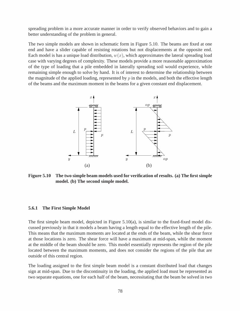
spreading problem in a more accurate manner in order to verify observed behaviors and to gain abetter understanding of the problem in general.

The two simple models are shown in schematic form in Figure 5.10. The beams are fixed at oneend and have a slider capable of resisting rotations but not displacements at the opposite end.Each model is has a unique load distribution,w(x), which approximates the lateral spreading loadcase with varying degrees of complexity. These models provide a more reasonable approximationof the type of loading that a pile embedded in laterally spreading soil would experience, whileremaining simple enough to solve by hand. It is of interest todetermine the relationship betweenthe magnitude of the applied loading, represented byp in the models, and both the effective lengthof the beams and the maximum moment in the beams for a given constant end displacement.

y

L

x

p

p

x

L

y

p

p

αp

αp

(a) (b)

Figure 5.10 The two simple beam models used for verification of results. (a) The first simplemodel. (b) The second simple model.

5.6.1 The First Simple Model

The first simple beam model, depicted in Figure 5.10(a), is similar to the fixed-fixed model dis-cussed previously in that it models a beam having a length equal to the effective length of the pile.This means that the maximum moments are located at the ends ofthe beam, while the shear forceat those locations is zero. The shear force will have a maximum at mid-span, while the momentat the middle of the beam should be zero. This model essentially represents the region of the pilelocated between the maximum moments, and does not consider the regions of the pile that areoutside of this central region.

The loading assigned to the first simple beam model is a constant distributed load that changessign at mid-span. Due to the discontinuity in the loading, the applied load must be represented astwo separate equations, one for each half of the beam, necessitating that the beam be solved in two

78

sections. For this model, the governing differential equation of bending can be written as

EId4v

dx4=

−w1(x) = −p for 0 < x <L

2

−w2(x) = p forL

2< x < L

(5.3)

These expressions can then be solved in order to obtain the displacement of the beam under theprescribed load case. The following expressions result from integrating Equation (5.3).

EIv1(x) = − p

24x4 +

c16x3 +

c22x2 +

c32x+ c4 (5.4a)

EIv2(x) =p

24x4 +

c56x3 +

c62x2 +

c72x+ c8 (5.4b)

In order to solve for the eight unknown constants, four boundary conditions and four compatibilityconditions must be enforced. These boundary conditions are

v1(x = 0) = 0 (5.5a)

dv1dx

∣

∣

∣

∣

x=0

= 0 (5.5b)

dv2dx

∣

∣

∣

∣

x=L

= 0 (5.5c)

VL = EId3v2dx3

∣

∣

∣

∣

x=L

= 0 (5.5d)

The compatibility conditions, which describe the relationship between the two halves of the beamat the point where they meet, can be expressed as

v1

(

x =L

2

)

= v2

(

x =L

2

)

(5.6a)

dv1dx

∣

∣

∣

∣

x=L

2

=dv2dx

∣

∣

∣

∣

x=L

2

(5.6b)

M1,L/2 = EId2v1dx2

∣

∣

∣

∣

x=L

2

= EId2v2dx2

∣

∣

∣

∣

x=L

2

=M2,L/2 (5.6c)

V1,L/2 = EId3v1dx3

∣

∣

∣

∣

x=L

2

= EId3v2dx3

∣

∣

∣

∣

x=L

2

= V2,L/2 (5.6d)

Applying the boundary and compatibility conditions of Equations (5.5) and (5.6), the unknownconstants in Equation (5.4) can be determined. This resultsin the following expression for the

79

−0.01 0 0.030

0.1

0.2

0.3

0.4

0.5

0.6

0.7

0.8

0.9

1

x/L

−0.4 00

0.1

0.2

0.3

0.4

0.5

0.6

0.7

0.8

0.9

1

−0.1 0 0.10

0.1

0.2

0.3

0.4

0.5

0.6

0.7

0.8

0.9

1

∆EI

pL4

V

pL

M

pL2

x/L

Figure 5.11 Displaced shape, shear diagram, and moment diagram for the first simplemodel.

displacement in the beam for the first simple model

v1(x) =pL4

48EI

[

3(x

L

)2

− 2(x

L

)4]

(5.7a)

v2(x) =pL4

192EI

[

8(x

L

)4

− 32(x

L

)3

+ 36(x

L

)2

− 8(x

L

)

+ 1

]

(5.7b)

The displaced shape for the first simple model described by Equation (5.7), along with the cor-responding expressions for the moment and shear in the beam,are plotted in Figure 5.11 usingthe shown dimensionless parameters. As shown, the maximum moments in the beam occur atthe boundaries of the model and the maximum shear force occurs in the middle. This coincideswith the intention of the first simple model to represent onlythe effective length,Leff , of the pilesubjected to the lateral spreading load case.

The maximum displacement, as shown in Figure 5.11, occurs atthe positionx = L. Substitutingthis into Equation (5.7b) defines the end displacement,∆, as

∆ = v2 (L) =5pL4

192EI(5.8)

wherep is the magnitude of the applied load,EI is the beam stiffness, andL is the beam length.Recalling that for this simple model, the length of the beam is equal to the effective length,Leff ,

80

for the lateral spreading load case, Equation (5.8) can be rearranged in order to obtain an expressionfor the effective length of the beam in terms of∆, p, andEI.

Leff =

(

192EI∆

5p

)0.25

(5.9)

The maximum moment in the beam can be determined in a similar manner. Evaluating the momentequation atx = L gives an expression for the absolute value of the maximum moment in the beamof the form

maxM =pL2

8(5.10)

The expressions developed in Equations (5.9) and (5.10) canbe used to explore the relationshipsbetween the effective length and maximum moment of the beam with the magnitude of the appliedload.

5.6.2 The Second Simple Model

The second simple model expands the relatively basic concept behind the first model to include abeam that represents the entire length of the pile in the lateral spreading model and a distributedloading that varies in magnitude with position. The second simple beam model is schematicallydepicted in Figure 5.10(b). In a way, this model is a rough approximation of the load distributionresulting from the imposed displacement profile of the 3D lateral spreading model in the caseswhere the piles are entirely elastic. Notice the similarityof this assumed distribution to that re-turned from the2.5-m-diameter pile in elastic soil shown in Figure 5.5.

As with the first model, the base of the beam is fixed while the opposing end of the beam is assigneda slider. In the second simple beam model, the maximum momentwill not occur at the ends of thebeam, instead, the moment should be zero at the ends. The maximum moment will occur at somelocation between the mid-span and end of the beam, with the exact location depending upon theassigned beam and load parameters. The shear force in the beam should still be zero at the endsand have a maximum at the center of the beam.

The distributed load acting upon the beam varies linearly with position, increasing in the lowersection of the beam from a somewhat arbitrary value of -αp at the base to a value ofp at mid-span. This loading pattern is then mirrored in the second half of the beam, with the load increasinglinearly from a value of -p at the center toαp at the top. To increase the generality of this model,the coefficientα is used to represent a constant loading factor such that0 < α < 1. For most ofthe post-processing associated with this model,α = 0.5.

As with the first simple model, there is a discontinuity in theloading at mid-span. For this reason,the beam must be represented by two sets of equations, each existing only over its respective halfof the beam. For the second simple model the governing differential equation of bending can bewritten as

EId4v

dx4=

−w1(x) = −2p(1 + α)x

L+ αx for 0 < x <

L

2

−w2(x) = −2p(1 + α)x

L+ p(2 + α) for

L

2< x < L

(5.11)

81

Integrating these expressions to obtain the displacement of the beam results in

EIv1(x) = − p

60L(1 + α)x5 +

p

24αx4 +

c16x3 +

c22x2 +

c32x+ c4 (5.12a)

EIv2(x) = − p

60L(1 + α)x5 +

p

24(2 + α)x4 +

c56x3 +

c62x2 +

c72x+ c8 (5.12b)

For the second simple model, the boundary and compatibilityconditions are unchanged from thefirst simple model, a fact that can be verified through examination of Figure 5.10. Therefore,Equations (5.5) and (5.6) are applied to determine the unknown constants of Equation (5.12),resulting in the following expressions for the displaced shape of the beam

v1(x) =pL4

240EI

[

− 4(1 + α)(x

L

)5

+ 10α(x

L

)4

+ 5(1− 2α)(x

L

)2]

(5.13a)

v2(x) =pL4

960EI

[

− 16(1 + α)(x

L

)5

+ 40(2 + α)(x

L

)4

− 160(x

L

)3

+ 20(7− 2α)(x

L

)2

− 40(x

L

)

+ 5

]

(5.13b)

The displaced shape and distributions of shear force and bending moment in the second model areshown in Figure 5.12 using the shown dimensionless parameters. The coefficientα is assigneda value of one-half. These plots verify that the second simple model accomplishes its goal ofapproximating the loading applied to a pile in the lateral spreading model. The shear force iszero at each end with a maximum in the center of the beam, and the moment has maximumswhere the shear is zero, occurring at a location between the center and the end of the beam. Thedistributions of both moment and shear for this model are fairly similar to those developed in thelateral spreading model The results from the simple models are more uniform due to the prescribedload distribution, but they share the same general shape as their more complex counterparts.

An expression for the end displacement,∆, occurring at the positionx = L (the top of the beam),is determined from Equation (5.13b) as

∆ =(9− 16α)pL4

960EI(5.14)

To determine the effective length for the second simple model, the location of the maximum mo-ment is computed in each segment of the beam. This is accomplished by determining the locationsin which the shear force is zero. These locations are

ξ1 =α

1 + αfor 0 < ξ1 <

1

2(5.15a)

ξ2 =1

1 + αfor

1

2< ξ1 < 1 (5.15b)

82

0 0.0010

0.1

0.2

0.3

0.4

0.5

0.6

0.7

0.8

0.9

1

x/L

−0.1 0 0.050

0.1

0.2

0.3

0.4

0.5

0.6

0.7

0.8

0.9

1

−0.01 0 0.010

0.1

0.2

0.3

0.4

0.5

0.6

0.7

0.8

0.9

1

∆EI

pL4

V

pL

M

pL2

Leffx/L

Figure 5.12 Displaced shape, shear diagram, and moment diagram for the second simplemodel.

The effective length of the beam is found as

Leff

L= min

{

1,min

{

ξ2,1

2

}}

−max

{

0,min

{

ξ1,1

2

}}

(5.16)

which defines the effective length for any value of the coefficient α. The maximum moment inthe beam is determined by evaluating the moment equation at the previously obtained locations ofmaximum moment. For values ofα which satisfy the conditions of Equation (5.15), the maximummoment in the beam can be expressed as

maxM =pL2α3

6(1 + α)2+pL2

24(1− 2α) (5.17)

5.6.3 Observations

When elastoplastic soil elements are used in the lateral spreading model, there is a limit to theamount of resistance the soil will provide. In the areas where yielding occurs, such as near theliquefied layer, the load on the pile increases as the contactzone between the soil and pile increasesin length. In the simple models, this behavior could be represented as an increase in the magnitudeof p. In order to gain insight from the two simple models, plots ofp versus the effective length ofthe beam andp versus the maximum moment in the beam are made for each simplebeam modelfor a constant end displacement,∆.

83

0 0.2 0.4 0.6 0.8 10

2

4

6

8

10

p

L eff

p−Leff

for first simple model

0 0.2 0.4 0.6 0.8 10

2

4

6

8

10

p

L eff

p−Leff

for second simple model with α = 0.50

0 0.2 0.4 0.6 0.8 10

0.1

0.2

0.3

0.4

0.5

0.6

0.7

0.8

p

max

M

p−maxM for first simple model

0 0.2 0.4 0.6 0.8 10

0.05

0.1

0.15

0.2

0.25

p

max

M

p−maxM for second simple model with α = 0.50

Figure 5.13 Normalized relationships betweenLeff , maxM , and p for the two simple mod-els.

The plots of Figure 5.13 show the variation in the key bendingparameters, effective length,Leff ,and maximum moment,maxM , with the magnitude of the applied loading,p, for a constant enddisplacement of∆ = 1. In all of the plots of Figure 5.13, dimensionless analysis is used toallow the curves to be shown in a normalized manner. For increasing values ofp, the effectivelength of each model decreases while the maximum moment in the models increases. This is thesame behavior observed for all three elastic pile models in the 3D lateral spreading simulations,attainable from models easily solved by hand.

It has been shown that the two simple beam models are able to approximate the behavior of thepiles in the three-dimensional lateral spreading model. Both Figures 5.11 and 5.12 show momentand shear diagrams that are reasonably similar to the momentand shear diagrams resulting fromthe lateral spreading model. With this reassurance, it is concluded that the behavior of these modelsis representative of the behavior of the piles due to the imposed displacement profile. The observedtendency for increasing maximum moment and decreasing effective length for increasing magni-

84

tudes of the applied load distribution in the simple models verifies that the lateral spreading resultsare reasonable while also offering a mechanism for this behavior. These models may also be usefulas a quick method to predict approximate demands for a pile subject to lateral spreading.

5.7 SUMMARY

During a lateral spreading event, an embedded pile foundation fundamentally alters the deforma-tion of the soil system while simultaneously undergoing deformation of its own. Many factorscontribute to the resultant behavior of the pile and the surrounding soil, among them the bendingstiffness of the pile as compared to the lateral stiffness ofthe soil, the ultimate strength of both thepile and the soil, as well as the degree of fixity at the extentsof the pile.

When the soil-pile system is modeled as entirely linear elastic, fundamental behavioral mecha-nisms can be observed in the system. As the lateral movement of the upper soil layer progresses,the pile embedded in the soil is pushed in the direction of flow. Depending upon the magnitudeof the ratio of the pile’s bending stiffness to the lateral stiffness of the soil, the pile also offersresistance to the lateral flow of soil, with greater resistance provided by those piles with the largeststiffness ratios. The bending demands which are generated in the piles follow consistent patternsfor all pile sizes with the maximum shear force demand developing at the center of the liquefiedlayer due to the change in sign of the applied loading, and themaximum moment demands fallingsomewhat outside the boundaries of the liquefied layer, withone extreme value in each of the twosolid soil layers. The distance between the maximum momentsdefines the effective length of thepile,Leff , a parameter which provides an indication of the severity ofthe bending demand.

By altering the soil constitutive model to consider plasticbehavior, the amount of load that thepile must carry increases, leading to increased bending demands when compared to the linearelastic models. This phenomenon has been verified through the use of simple beam models. Inaddition to changing the relationship between the pile and the soil, considering elastoplastic soilbehavior allows for the observation of the ways in which the weaker liquefied layer affects thesurrounding solid soil layers. As the pile is pushed into thesoil, the solid soil near the boundary ofthe liquefied layer is able to be pushed into the adjacent liquefied layer, thus effectively reducingthe lateral resistance of the soil in the regions near the liquefied layer. This final aspect of thebehavior observed in the system is critical to the lateral spreading problem and is explored furtherin Chapter 8.

85

6 Computation of Representative p– y Curvesfrom the Three-Dimensional Model

6.1 INTRODUCTION

In current geotechnical engineering practice, it is commonto analyze a pile foundation subject tolateral loads as a beam on a nonlinear Winkler foundation. Itis therefore of interest to develop alateral spreading analysis procedure that is compatible with this current design paradigm. Repre-sentativep –y curves are computed from 3D FE analysis in order to evaluate the applicability ofthis approach to the lateral spreading problem. To this purpose, a reliable method for computingthep –y curves must be established.

The computational process includes identifying the appropriate data recorded during the 3D sim-ulations as well as evaluating the effects of various factors on the resultingp –y curves. Investiga-tions are made into the ways in which the pile deformation pattern (pile kinematics), the selectivemesh refinement scheme employed in the models, and the location of the fixed boundaries af-fect the computedp –y curves. It is determined that all three of these factors are influential andsolutions to properly handle their respective effects are proposed.

6.2 COMPUTATION OF FORCE AND DISPLACEMENT HISTORIES

Computing a set ofp –y curves from the 3D FE model requires knowledge of the force and dis-placement histories for the pile nodes. The general computational process is shown in Figure 6.1.The forces exerted on the pile by the surrounding soil are determined directly from the beam-solidcontact elements (Petek, 2006), which integrate the 3D interface tractions applied by the soil to theouter surface of the pile into a force vector at each pile node. By recording this vector, the resultantforce components acting in the direction of loading are defined at each of the pile nodes.

Due to the symmetry condition present in the model, the magnitudes of these force components re-flect only one-half of the full pile circumference. To obtainresults consistent with the full diameterof the piles, these forces are doubled. In order to obtain mesh-independent values, each force mustalso be normalized by the tributary length of pile over whichit acts. For each respective pile node,the tributary length is defined as half the distance to the adjacent pile nodes in either direction. Forthe end nodes, the tributary length is half the distance to the sole adjacent node.

87

Interface forces

∆

f(z, θ)

f(z, θ)z

Pile

locationoriginal pile

tributarylength

yi fi

p – y curvesResultant forces on pilepi = fi/ℓi

Discretized

pi

yi

fi =∮

f(z, θ)rdθ

ℓi

Figure 6.1 Computation ofp –y curves from the 3D FE model.

The desired displacement for generation ofp –y curves representative of the soil response is thedifferential displacement between the pile and the soil. Inthe case of the lateral spreading models,the displacement values recorded directly from the pile arenot a measure of the distance that thepile is pushed into the surrounding soil, but a measure of theactual displacement experienced bythe pile. To obtain the displacement of the pile relative to the surrounding soil for this case, theimposed far-field soil displacement profile is subtracted from the pile displacement profile recordedby the model, as schematically in Figure 6.2. For analyses inwhich all or part of the pile is directlypushed into the surrounding soil, this subtraction procedure is not required as the recorded piledisplacements are the relative displacements between the pile and the surrounding soil.

undeformed pilecenterline

pile displacementprofile

profiledisplacementimposed soil

p-y displacement

Figure 6.2 Determination of displacements suitable for usein p - y curves for the lateralspreading case.

88

∆ ∆ ∆

(c)(b)(a)

Figure 6.3 Pile kinematic cases. (a) Lateral Spreading; (b)Top pushover; (c) Rigid pile.

6.3 CONSIDERED KINEMATIC CASES

Three separate pile deformation patterns are considered inorder to provide a means to evaluate theeffects of varying pile kinematics on thep –y curves resulting from the FE analysis. These casesinclude the following: (1) a lateral spreading case, Figure6.3(a), which is the primary focus ofthis research; (2) a top pushover case, Figure 6.3(b), matching the type of test used to empiricallyderivep –y curves; and (3) a rigid pile case, Figure 6.3(c), in which thepile is pushed a uniformlateral distance into the soil.

The top pushover case simulates a displacement controlled lateral load test. The top node of thepile is displaced laterally in the symmetry plane while all other pile nodes are free to translate androtate in this plane. The pile head is left to rotate freely. This kinematic mode results in largedeformations near the surface and small deformations at greater depths. For the rigid pile case, allpile nodes are translated laterally into the soil without rotation; the remaining boundary conditionson the soil are unchanged.

All three kinematic cases are modeled using the FE mesh used in the 3D lateral spreading sim-ulations. The piles are modeled using the linear elastic formulation discussed in Section 3.4.Elastoplastic soil behavior is considered using the Drucker-Prager constitutive model discussedin Section 4.4. All three of the template pile designs are considered.

6.4 CURVE-FITTING STRATEGIES

The p –y data returned from the simulations is a set of discrete points representing the force,normalized by element length, applied to the pile at specificvalues of displacement. In orderto manipulate and analyze this data mathematically, curvesmust be fitted to the data points toobtain smooth and continuous functions that describe thep –y curve at each node. To this end,a least squares curve-fitting strategy is employed for two separate functional forms, a polynomialfunction and a hyperbolic tangent function. The polynomialfunction is utilized to estimate theinitial tangent for thep –y curves, while the hyperbolic tangent function is used to describe the

89

shape of thep –y curves and to define the ultimate resistance of each curve. Because the forcesand displacements may be positive or negative, depending upon the specific deformation pattern ineach case, the absolute values of the forces and displacements are used for curve-fitting purposes.

6.4.1 Hyperbolic Tangent Function

A hyperbolic tangent function is chosen to allow direct comparison to the API (1987) recommen-dations, which describe the shape ofp –y curves for cohesionless soils using this functional form.The fitted function has the form

p(y) = pu tanh

(

kz

puy

)

(6.1)

in which z is the depth and the parameterk, with units of force/length3, affects the slope of thefunction. Equation (6.1) defines the two characteristic parameters used to compare and evaluatesets ofp –y curves: (1) the ultimate lateral resistance,pu; and (2) the initial tangent stiffness,kT = dp(y)/dy|y=0.

Least squares is used to determine the constantspu andk for thep –y data at each pile node. ForEquation (6.1), the residual,rj , at each pile node can be expressed as the difference betweenthevalue returned from the simulation and that estimated by thecurve-fitting function.

rj = pj − pu tanh

(

kz

puyj

)

(6.2)

The best fit for the data is achieved when the error is at a minimum. For this problem, the errorfunction is obtained as

E(pu, k) =∑

j

1

2r2j =

∑

j

[

pj − pu tanh

(

kz

puyj

)]2

(6.3)

The error is at a minimum when its gradient is zero. Because there are two parameters, it isexpedient to perform the solution in vector form by defining the vectorλ with two componentsλ1 = pu andλ2 = k. The gradient equations can thus be written in terms of this vector,λ, as

∂E∂λi

=∑

j

rj∂rj∂λi

= 0 (6.4)

The necessary derivatives of the residual with respect to the two parametersλ1 andλ2 can beexpressed as

∂rj∂λ1

=∂rj∂pu

=kz

puyj sech2

(

kz

puyj

)

− tanh2

(

kz

puyj

)

= 0 (6.5)

∂rj∂λ2

=∂rj∂k

= −zyj sech2(

kz

puyj

)

= 0 (6.6)

90

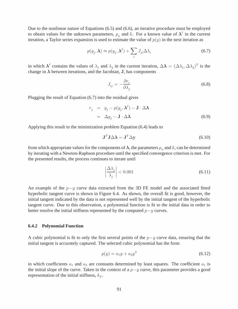
Due to the nonlinear nature of Equations (6.5) and (6.6), an iterative procedure must be employedto obtain values for the unknown parameters,pu andk. For a known value ofλℓ in the currentiteration, a Taylor series expansion is used to estimate thevalue ofp(y) in the next iteration as

p(yj,λ) ≈ p(yj,λℓ) +

∑

i

Jji∆λi (6.7)

in which λℓ contains the values ofλ1 andλ2 in the current iteration,∆λ = (∆λ1,∆λ2)T is the

change inλ between iterations, and the Jacobian,J, has components

Jij = − ∂ri∂λj

(6.8)

Plugging the result of Equation (6.7) into the residual gives

rj = yj − p(yj,λℓ)− J ·∆λ

= ∆yj − J ·∆λ (6.9)

Applying this result to the minimization problem Equation (6.4) leads to

JTJ∆λ = JT∆y (6.10)

from which appropriate values for the components ofλ, the parameterspu andk, can be determinedby iterating with a Newton-Raphson procedure until the specified convergence criterion is met. Forthe presented results, the process continues to iterate until

∣

∣

∣

∣

∆λjλj

∣

∣

∣

∣

< 0.001 (6.11)

An example of thep –y curve data extracted from the 3D FE model and the associated fittedhyperbolic tangent curve is shown in Figure 6.4. As shown, the overall fit is good, however, theinitial tangent indicated by the data is not represented well by the initial tangent of the hyperbolictangent curve. Due to this observation, a polynomial function is fit to the initial data in order tobetter resolve the initial stiffness represented by the computedp –y curves.

6.4.2 Polynomial Function

A cubic polynomial is fit to only the first several points of thep –y curve data, ensuring that theinitial tangent is accurately captured. The selected cubicpolynomial has the form

p(y) = a1y + a3y3 (6.12)

in which coefficientsa1 anda3 are constants determined by least squares. The coefficienta1 isthe initial slope of the curve. Taken in the context of ap –y curve, this parameter provides a goodrepresentation of the initial stiffness,kT .

91

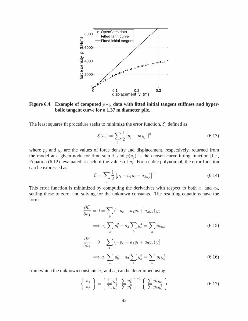
0 0.1 0.2 0.30

2000

4000

6000

8000

displacement y (m)

forc

e de

nsity

p (

kN/m

)

OpenSees dataFitted tanh curveFitted initial tangent

Figure 6.4 Example of computedp –y data with fitted initial tangent stiffness and hyper-bolic tangent curve for a 1.37 m diameter pile.

The least squares fit procedure seeks to minimize the error function,E , defined as

E(ai) =∑

j

1

2[pj − p(yj)]

2 (6.13)

wherepj and yj are the values of force density and displacement, respectively, returned fromthe model at a given node for time stepj, andp(yj) is the chosen curve-fitting function [i.e.,Equation (6.12)] evaluated at each of the values ofyj. For a cubic polynomial, the error functioncan be expressed as

E =∑

j

1

2

[

pj − a1yj − a3y3j

]2(6.14)

This error function is minimized by computing the derivatives with respect to botha1 anda3,setting these to zero, and solving for the unknown constants. The resulting equations have theform

∂E∂a1

= 0 =∑

k

(−pk + a1yk + a3yk) yk

=⇒ a1∑

k

y2k + a3∑

k

y4k =∑

k

pkyk (6.15)

∂E∂a3

= 0 =∑

k

(−pk + a1yk + a3yk) y3k

=⇒ a1∑

k

y4k + a3∑

k

y6k =∑

k

pky3k (6.16)

from which the unknown constantsa1 anda3 can be determined using{

a1a3

}

=

[∑

y2k∑

y4k∑

y4k∑

y6k

]

−1{ ∑

pkyk∑

pky3k

}

(6.17)

92

An example of the fitted initial tangent stiffness provided by the cubic polynomial is shown inFigure 6.4. This stiffness is a much better representation of the initial tangent indicated by thedata. For all subsequent discussion, it can be assumed that any reference made to the initial tangentstiffness,kT , of thep –y curves refers to that obtained using the cubic polynomial. All values ofthe ultimate lateral resistance,pu, are determined from the fitted hyperbolic tangent functions.

6.5 EFFECTS OF PILE KINEMATICS ON COMPUTED p –y CURVES

The rigid pile case, Figure 6.3(c), is used as a benchmark to evaluate the effects of pile kinematicson p –y curves. This case eliminates the influence of pile deformation on the computed curvesand activates the soil response consistently at all depths.Thep –y curves resulting from the lat-eral spreading, Figure 6.3(a), and top pushover, Figure 6.3(b), cases are generally comparable tothose resulting from the rigid pile case, however, in certain locations the curves deviate from thebenchmarks. This observation underscores a potential flaw in the assumption that representativep –y curves can be extracted from the 3D finite element model without exception and identifies theneed for a more careful approach top –y curve computation.

The lateral spreading, Figure 6.3(a), and top pushover, Figure 6.3(b), cases are compared to thebenchmark case with respect to and initial stiffness ratio (kT ratio), and a lateral resistance ratio(LRR). The initial stiffness ratio is computed by dividing the initial tangent stiffness,kT , in thevariable kinematic cases, i.e., top pushover and lateral spreading, by the corresponding value ofkTin the rigid pile case. Because there are locations at which the displacements are very small andlittle soil resistance is mobilized, ultimate lateral resistances are not compared in this study.

The LRR compares the resistance provided at a specified levelof lateral displacement for a givenkinematic case to that provided at the same level of displacement for the benchmark case. Thiscomparative means was used in a similar manner by Yang and Jeremic (2005) in their work with3D FE analysis of layered soil profiles. An example of how the LRR works is illustrated in Fig-ure 6.5. Four displacement increments are investigated in this study in an effort to gauge howthe relationships between the curves may vary over time. TheLRR is computed at displacementsequal to0.5%, 1%, 2%, and4% of the pile diameter in each respective case.

p1

p2

p

LRR =p1p2

yref y

Figure 6.5 The lateral resistance ratio, LRR, is the ratio ofthe soil resistance values com-puted in two referencep –y curves at a prescribed value of displacement.

93

Table 6.1 Overview of the four considered kinematic comparison cases.

Rigid Top Pushover Lateral SpreadHomogenous Soil X XLayered (Liquefied) Soil X X

Table 6.1 provides a brief overview of the four kinematic comparison cases considered for each pilediameter. The top pushover case is run in an entirely homogeneous soil system, while the lateralspreading case is run in the three-layer liquefied soil modeldiscussed previously. The results ofthese two variable kinematic cases are compared to a rigid pile analysis in a corresponding soilprofile.

ComputedkT ratios and LRR’s are presented in Figures 6.6 and 6.7 for the the lateral spreading andtop pushover kinematic cases, respectively, for a 1.37-m- diameter pile. These results are typical ofall considered piles. The evolution of the differential displacement between the pile and the soil isincluded to provide a context for the deformation pattern with depth. The depth and displacementscales are normalized by pile diameter.

If the resistance indicated by thep –y curves depended only on relative soil-pile displacement, asassumed in the Winkler model, both thekT ratio and LRR would be equal to1.0. Figures 6.6and 6.7 show that thekT ratio and LRR deviate significantly from1.0, hence, there are significantdifferences in thep –y curves computed from the different pile kinematics.

Aside from the top few diameters of the top pushover comparisons, which are affected by interac-tion with the free surface, areas in which the displacement is large show good agreement betweenthe respectivep –y curves. However, significant deviations occur in the areas in which the dis-placements are relatively small. At a particular depth, thep –y curves for the lateral spreading andtop pushover cases vary with respect to the rigid pile results based upon the magnitude of the piledisplacement and how this displacement changes during the analysis.

Similar observations are made when looking at comparisons between the actualp –y curves com-puted from the simulations. A selection of computedp –y curves for a 0.61-m-diameter pile isshown in Figures 6.8 and 6.9. As shown, there are locations inwhich the curves match well andlocations in which they do not. These plots also demonstratethe inadequacy of the top pushoverand lateral spreading cases in the activation of the ultimate resistance of the soil, leading to theconclusion that a reasonable estimate ofpu is not possible for these cases.

Differing results for different kinematic cases are observed for all three pile diameters. The areas ofgreatest divergence do not occur at the same depth for different piles, therefore, depth or meshingeffects can be ruled out as the causes of the difference. For all cases, the only difference betweenthe compared analyses is the pile kinematics, thus, the observed differences must be attributable tothis factor. An explanation for this observation is offeredby way of the Betti-Rayleigh theorem ofreciprocal work (Megson, 2005).

94

−0.2 0 0.2−20

−18

−16

−14

−12

−10

−8

−6

−4

−2

0

0 1 2−20

−18

−16

−14

−12

−10

−8

−6

−4

−2

0

0 1 2−20

−18

−16

−14

−12

−10

−8

−6

−4

−2

0

−4

−14

−4

−14

0

−2

−6

−8

−10

−12

−16

−18

−20

−4

−14

0

−2

−6

−8

−10

−12

−16

−18

−20

−4

−14

−4

−14

normalizeddisplacement

norm

aliz

ed d

epth

−0.2 0 0.2 0 01 2 1 2LRRk ratioT

0

−6

−8

−10

−12

−16

−18

−20

−2

kinematiccase

y/D = 0.5%y/D = 1.0%y/D = 2.0%y/D = 4.0%

Figure 6.6 Comparison of the lateral spreading kinematic case to the rigid pile case for a1.37-m-diameter pile. Both analyses use a three-layer liquefied soil system.

−0.2 0 0.2−20

−18

−16

−14

−12

−10

−8

−6

−4

−2

0

0 1 2−20

−18

−16

−14

−12

−10

−8

−6

−4

−2

0

0 1 2−20

−18

−16

−14

−12

−10

−8

−6

−4

−2

0

0 0.5 1−20

−18

−16

−14

−12

−10

−8

−6

−4

−2

0

0 1 2−20

−18

−16

−14

−12

−10

−8

−6

−4

−2

0

0 1 2−20

−18

−16

−14

−12

−10

−8

−6

−4

−2

0

−4

−14

−4

−14

0

−2

−6

−8

−10

−12

−16

−18

−20

−4

−14

0

−2

−6

−8

−10

−12

−16

−18

−20

−4

−14

−4

−14

normalizeddisplacement

norm

aliz

ed d

epth

0 01 2 1 2LRRk ratioT

0

−6

−8

−10

−12

−16

−18

−20

−2

0.50 1kinematic

case

y/D = 0.5%y/D = 1.0%y/D = 2.0%y/D = 4.0%

Figure 6.7 Comparison of the top pushover kinematic case to the rigid pile case for a a1.37-m-diameter pile. Both analyses use homogenous soil profiles.

95

0 0.05 0.1 0.150

500

1000

1500

2000

Horizontal displacement in (m)

Hor

izon

tal f

orce

/leng

th in

(kN

/m)

3.42 m below surface

Rigid PileTop PushoverRigid Pile Initial TangentTop Pushover Initial Tangent

0 0.05 0.1 0.150

500

1000

1500

2000


Hor

izon

tal f

orce

/leng

th in

(kN

/m)



0 0.05 0.1 0.150

500

1000

1500

2000


Hor

izon

tal f

orce

/leng

th in

(kN

/m)



0 0.05 0.1 0.150

500

1000

1500

2000


Hor

izon

tal f

orce

/leng

th in

(kN

/m)



0 0.05 0.1 0.150

500

1000

1500

2000


Hor

izon

tal f

orce

/leng

th in

(kN

/m)



0 0.05 0.1 0.150

500

1000

1500

2000


Hor

izon

tal f

orce

/leng

th in

(kN

/m)



Figure 6.8 Computedp –y curves from the top pushover and rigid pile cases in homogenoussoil for a 0.61-m-diameter pile. The fitted initial tangentsare shown for eachcase.

96

0 0.05 0.1 0.150

500

1000

1500

2000


Hor

izon

tal f

orce

/leng

th in

(kN

/m)


Rigid PileTop PushoverRigid Pile Initial TangentLateral Spread Initial Tangent

0 0.05 0.1 0.150

500

1000

1500

2000


Hor

izon

tal f

orce

/leng

th in

(kN

/m)



0 0.05 0.1 0.150

500

1000

1500

2000


Hor

izon

tal f

orce

/leng

th in

(kN

/m)



0 0.05 0.1 0.150

500

1000

1500

2000


Hor

izon

tal f

orce

/leng

th in

(kN

/m)



0 0.05 0.1 0.150

500

1000

1500

2000


Hor

izon

tal f

orce

/leng

th in

(kN

/m)



0 0.05 0.1 0.150

500

1000

1500

2000


Hor

izon

tal f

orce

/leng

th in

(kN

/m)



Figure 6.9 Computedp –y curves from the lateral spreading and rigid pile cases in non-homogenous soil for a 0.61-m-diameter pile. The fitted initial tangents are shownfor each case.

97

6.5.1 Betti-Rayleigh Theorem of Reciprocal Work

The Betti-Rayleigh theorem of reciprocal work is a principle which relates the work done by twoseparate load cases acting on a linear elastic body. Consider the elastic body of Figure 6.10 whichdepicts two separate load cases,P andQ, acting on the same points of the body, and their respectivedisplacements,u andv.

caseP caseQ

u1

u2

u3

P2

P3

Q1

v1

Q2

v2

v3

Q3

P1

Figure 6.10 Two separate load cases,P and Q, with respective displacements,u and v,applied to the same points on a general elastic body.

The reciprocal theorem states that the work done by loadsPi when moving through the displace-ments produced by loadsQj is equal to the work done by loadsQj when moving through the dis-placements produced by loadsPi (Megson, 2005). The Betti-Rayleigh theorem can be expressedusing the dot product as

∑

i

Pi · vi =∑

j

Qj · uj (6.18)

6.5.2 Application of the Betti-Rayleigh Theorem

To apply this theorem to the problem of a laterally loaded pile, it is convenient to designate loadcaseP as the nodal forces applied to a pile havingn nodes as its passage is resisted by the sur-rounding soil, indicating thatu is the corresponding vector of nodal displacements. These are theterms that are related to each other to generate thep –y curves at each pile node. If load caseQ isa unit load applied at an arbitrary node,j, on the pile, thenv represents the corresponding nodaldisplacements for this load and (6.18) can be written as

P1v1 + P2v2 + . . . Pnvn = uj (6.19)

from which a full set of equations can be written, in matrix form, as

[A]{P} = {u} (6.20)

in whichP carries the lateral pile forces,u contains the lateral pile displacements, and the com-ponentsAij are the displacements at each nodei produced by a unit load at nodej. SolvingEquation (6.20) for the nodal forces results in

{P} = [A]−1{u} (6.21)

98

which can be evaluated for the force,Pj acting at an arbitrary nodej as

Pj = A−1j1 u1 + A−1

j2 u2 + . . . A−1jn un (6.22)

whereA−1ji represents the components of[A]−1.

The effects of pile kinematics on thep –y curve extraction procedure can be drawn from Equa-tion (6.22) by considering what happens when the displacement at nodej is varied in each kine-matic case. In the top pushover and lateral spreading cases,if uj is large, the force acting at nodejis largely dependent uponuj as the contribution by the termA−1

jj uj in Equation (6.22) is dominant

Pj = A−1j1 u1 + A−1

j2 u2 + . . . A−1jn un ≈ A−1

jj uj (6.23)

In this case, the assumption that there is a one-to-one relationship between the force and dis-placement at a node is relatively good, even though it is still an approximation. The regions ofFigures 6.6 and 6.7 in which thekT and lateral resistance ratios are nearly unity coincide with theareas in which the displacements are large, thereby supporting this explanation.

In contrast, great divergence between thep –y curves returned by the rigid and top pushover casesis observed in the regions where the displacements of the pile are small. Ifuj is small, then thecontributions to the force acting at nodej by the other terms in Equation (6.22) are no longerinsignificant, meaning that at such a point, the assumption of a local force-displacement relation-ship is relatively poor. This effect is exacerbated when thedisplacement at a particular node issmall compared to adjacent nodes at which the coefficients of[A] are relatively large. An exam-ple of this is most clearly made by looking at the middle sections of the lateral spreading cases.The nodes that are very near the center of the imposed displacement profile do not tend to movemuch during the entire process. The nodes just outside of this middle region undergo considerablylarger displacements into the surrounding soil, thus affecting the results for the nodes in the middleregion.

6.5.3 Proposed Solution to the Problem of Pile Kinematics

The findings discussed above suggest that the kinematics of the pile strongly influence the resultingp –y curves for the variable pile kinematic cases and this must beconsidered when attempting todefine a set of curves suitable for use in the analysis of a general pile deformation. The selectedp –y curves should reflect only the response of the soil, not a combination of the soil and pileresponses. The pile response effect should be captured by the numerical model of choice.

In the rigid pile case the displacements at each node are identical. In the context of the Betti-Rayleigh theorem, this indicates that the coefficients of[A] are the determining factor in the forceapplied at a given node. This creates a situation whereby theassumption of a direct relationshipbetween the forces and displacements at the individual nodes is relatively good, as[A] is diagonaldominant. This observation, and the fact that the pile does not deform, indicates that the rigidpile case producesp –y curves that are not influenced by pile kinematics. Therefore, these curvesreflect only the response of the soil. This is the benefit of the3D FE analysis in comparison tofull-scale field experiments. It will be shown thatp –y curves obtained from this pile kinematicproduce reasonable results when applied to lateral spreading.

99

6.6 EFFECTS OF SELECTIVE MESH REFINEMENT ON COMPUTED p –y CURVES

Examining the results for each of the kinematic cases, it is observed that there are fluctuations inthe distributions of initial stiffness,kT , and ultimate lateral resistance,pu, with depth in the locationof the liquefied layer. This behavior is present in all cases and for all piles, even those in which thesoil profile is entirely homogenous. Figures 6.7 and 6.6 involve the ratios of two cases run usingthe same selectively refined mesh and therefore do not display similar fluctuations. While theseratios are valuable evaluation tools, the actual values of the curve parameters must also be verifiedas sensible, otherwise any conclusions drawn from the ratios are meaningless. In order to gainconfidence in the computedp –y curves, the cause of the fluctuations must be discerned.

It is hypothesized that the selective mesh refinement schemeis responsible for altering the results.The areas of inconstancy in the parameter distributions correspond not only to the location of theliquefied layer, but to the areas of differential mesh refinement. Because the failure of a cohesion-less soil is governed by shear, it seems sensible to assume that the size of the elements will affectthe perceived stiffness that the elements display towards this failure mechanism. For example, inthe wedge-type soil failure mechanism that is common at shallower depths, all of the gauss pointsthat are aligned with the failure surface must have reached yield in their associated constitutivemodels for the model to display the global behavior. Changing the vertical size of the elementschanges the spacing of the gauss points and may alter the number of gauss points that must expe-rience local failure in order for the global failure to occur, thus, altering the response of the soil asa whole, and, subsequently, the computedp –y curves.

In order to test the hypothesis that the selective mesh refinement is responsible for the observedfluctuations in soil response, a uniform mesh is generated for each of the piles. This uniform meshhas the same outer dimensions and layout as the selectively refined meshes, however, the soil andpile elements are all uniformly sized in the vertical direction. Two rigid pile cases are run usingthis uniform model, one in a homogenous soil profile, and the other in a three-layer soil profilewith a liquefied center layer. Figure 6.11 shows the distributions ofkT andpu, respectively, overthe length of a 1.37-m-diameter pile in homogenous soil using the uniform and selectively refinedmeshes. As shown, both the stiffness and resistance values fluctuate in the center of the pile forthe selectively refined case. The uniform case does not display similar behavior. Instead, thedistributions resulting from the uniform mesh are smooth over the entire length of the pile. Theseresults support the hypothesis.

A solution is proposed to smooth the soil response in the selectively refined cases by using theresults of the uniform mesh cases. This solution is proposedin lieu of running all previouslyanalyzed cases a second time, using a uniform mesh, in order to obtain smooth soil responsewhile simultaneously losing the valuable mesh resolution at the liquefied interface. Instead of thatlaborious pursuit, the selectively refined results are smoothened through multiplication with theratio of the uniform and refined results obtained from a rigidpile in homogenous soil for eachdiameter. This proposed solution also allows for further verification of the hypothesis that theselectively refined mesh scheme is the cause of the fluctuations in soil response.

Figure 6.12 shows both the original and smooth distributions of initial stiffness and ultimate lateralresistance for several kinematic cases. For the ultimate resistance, only the rigid pile case is

100

0 0.5 1 1.5 2 2.5 3

x 104

−25

−20

−15

−10

−5

0

inital stiffness (kPa)

dept

h (

m)

Uniform MeshSelectively Refined Mesh

0 1000 2000 3000 4000 5000 6000 7000

−25

−20

−15

−10

−5

0

ultimate lateral resistance (kN/m)

dept

h (

m)

Uniform MeshSelectively Refined Mesh

Figure 6.11 Distributions of kT and pu for 1.37-m-diameter pile in homogenous soil profile.

0 1000 2000 3000 4000 5000 6000 7000

−25

−20

−15

−10

−5

0


dept

h (

m)

Unsmoothened ResultsSmoothened Results

(a)

0 0.5 1 1.5 2 2.5 3

x 104

−25

−20

−15

−10

−5

0


dept

h (

m)


0 1 2 3 4 5

x 104

−25

−20

−15

−10

−5

0


dept

h (

m)


(b) (c)

Figure 6.12 Examples of smoothing process on curve parameters for 1.37-m-diameter pile.(a) Distribution of pu from rigid pile in liquefied soil profile; b) Distributionof kT from rigid pile in liquefied soil profile; (c) Distribution of kT from toppushover in homogenous soil profile.

101

considered due to the inability of the alternate kinematic cases to fully activate the soil responseat all depths. As shown, the smoothing process, involving the ratios obtained using the rigid pilecases in homogenous soil profiles, is able to remove the fluctuations in the parameter distributionsfor each of the alternative pile kinematic cases.

Though the stiffness distribution itself is suspect for reasons related to the pile kinematics, Fig-ure 6.12(c) illustrates well the effect of the smoothing procedure. The presented case is a toppushover in an entirely homogenous soil profile. There are fluctuations in the data set in the areawhere the mesh is more refined (centered approximately at a depth of 14 m). Through multiplyingthe initial stiffness distribution from this top pushover case by the ratio of the uniform results tothe selectively refined results for the rigid pile case, the inconsistencies in the results are removed,creating a smooth distribution through the depths encompassed by the increased mesh resolution.

The results of Figure 6.12 demonstrate the effectiveness ofthe smoothing procedure and verifythe validity of the hypothesis with respect to the selectivemesh refinement. The use of a selec-tively refined mesh can affect the results of a 3D FE simulation, but through careful diagnosis andrecognition, these effects can be nullified in a relatively cheap and simple manner.

6.7 BOUNDARY EFFECTS ON SOIL RESPONSE

The FE models generated for the studies performed in this research are intended to include suffi-cient lateral extents such that the results are relatively unaffected by the fixed boundaries on theoutside surfaces of the mesh. In order to gauge the significance of the fixed boundaries on the soilresponse recorded in the models, a new mesh is generated having increased lateral extents. Thisextended mesh is shown in Figure 6.13. The extended mesh shares a layout with the standard meshused in the other aspects of this research, however, the soilelements are extended for an additionalten pile diameters in the direction of loading. By increasing the amount of soil between the pileand the fixed boundary, it is expected that the effects of the boundary on the lateral response of thesoil profile can be discerned. All of the analyses discussed herein involve the rigid pile kinematiccase.

The distributions of the characteristicp –y curve parameters are plotted in Figure 6.14. As couldbe expected, the initial stiffness values returned from thetwo meshes are very similar. The prox-imity of the boundary should not significantly affect the response of the soil at such low levels ofpile displacement. The differences between the two distributions are easily attributable to minorvariations in the meshing around the pile between the two models. The ultimate lateral resistance,however, displays a reduction in magnitude for the extendedmesh case as compared to the standardmesh case. This result confirms the suspicion that the fixed boundary is able to affect the resultsof the laterally-loaded pile models, at least with regards to the ultimate resistance provided by thesoil elements.

The value ofpu returned by the models reflects the maximum load that the pilecan exert on thesoil before failure. This parameter is directly related to failure of the soil surrounding the pile.The Drucker-Prager plasticity model has a pressure-dependent yield surface, indicating that as theconfining pressure on a particular element increases, thereis a corresponding increase in the yieldcapacity for that element. This indicates thatpu should increase with either increasing depth or

102

Figure 6.13 Laterally-extended mesh for 0.61-m-pile design.

with increasing confining stress. As the pile is pushed laterally, the soil elements must deform toaccommodate its passage. At shallow depths, the overburdenstress is relatively small, thus, thesoil elements are pushed outwards and upwards by its passage. The distribution of this soil heaveextends well in front of the pile, and to the side as well, as illustrated in Figure 6.15, which showsthe distribution of vertical displacement in the soil in a plan view.

At increased depth, the overburden pressure in the soil elements becomes larger due to both theself weight of the soil and the active pressure provided by the overlaying elements expandingupwards. The zone in which the soil elements are pushed upwards and outwards by the passageof the pile therefore reduces in areal extent with increasing depth, naturally forming a wedge-like shape of moving soil in front of the pile. This type of wedge failure can clearly be seen inFigure 6.16, which shows the distribution of positive vertical displacements in the extended meshmodel. The formation of the wedge affects the deeper soil elements by actively increasing theconfining pressure as it expands.

In the case of the standard mesh, shown in Figure 6.17, the proximity of the fixed boundary pre-vents the formation of a full wedge by limiting the forward movement of the soil elements. Theboundary also allows for larger compressive lateral stresses to develop. The overburden pressurecan be overcome more easily at deeper locations, leading to the increased magnitude in verticaldisplacements and the increased extents of this upwardly-moving zone displayed in Figure 6.17.

These increases in the volume of soil that is moved upwards and the magnitude of the verticaldisplacement leads to an increase in the confining pressure at lower depths, especially as comparedto the results obtained from the laterally extended mesh. The stress increase can be observed inFigures 6.18 and 6.19, which show the distributions of the first invariant of stress,I1 = σ1+σ2+σ3,in the two models. As shown, the first stress invariant is significantly larger in compression in thestandard mesh than in the extended mesh due to the proximity of the pile to the fixed boundary.The observed increase in the ultimate lateral resistance ofthe soil elements in the standard mesh

103

0 1 2 3 4 5 6

x 104

−12

−10

−8

−6

−4

−2

0

initial stiffness (kPa)

dept

h (

m)

Standard MeshExtended Mesh

0 1000 2000 3000 4000 5000 6000 7000

−12

−10

−8

−6

−4

−2

0


dept

h (

m)

Standard MeshExtended Mesh

Figure 6.14 Comparison ofp –y curve parameter distributions for extended and standardmeshes for a 0.61-m-diameter pile.

over that displayed by the extended mesh shown in Figure 6.14is attributable to the increasedconfining stresses in that model.

The increase in the estimated values ofpu associated with the use of the standard mesh is apparent,but is not necessarily significant. In the current simulations, the pile is not pushed sufficiently farinto the soil as to fully activate the ultimate resistance ofthe soil at depth. Due to this shortcoming,the obtained values ofpu in these locations are extrapolated by the curve-fitting procedure andmay not represent the true capacity of the soil. This observation, along with alternative plasticityformulations that alleviate the boundary effects, is analyzed and discussed in Chapter 7.

Figure 6.15 Plan view showing the distribution of vertical displacement (i.e., soil heave) inthe soil elements. The areas near the pile indicate the greatest magnitude ofdisplacement, while the constantly shaded areas near the boundaries have zerodisplacement.

104

Figure 6.16 Contour plot of vertical soil displacements in the extended mesh. Only upwarddisplacements are considered.

Figure 6.17 Contour plot of vertical soil displacements forthe rigid pile case in the standardmesh. Only upward displacements are considered.

105

Figure 6.18 Distribution of the first invariant of stress, I1, in the standard mesh for a 0.61-m-diameter pile.

Figure 6.19 Distribution of the first invariant of stress, I1, in the extended mesh for a 0.61-m-diameter pile.

106

6.8 SUMMARY

It is of interest to evaluate the results obtained using 3D FEmodels of piles embedded in laterallyspreading soils in the context of the commonly usedp –y method. In order to accomplish thisgoal, a method in which to extract reliable and sensiblep –y curves was developed. Least squaresis used to fit functions to the computed data in order to describe the computedp –y curves and toidentify the key curve parameters of initial stiffness,kT , and ultimate lateral resistance,pu.

It is determined that the pile kinematics in these simulations play an important role in defining thesuccess rate forp –y curve extraction from the FE model. It is observed that in addition to theknown effects of differential soil layer strength on thep –y curves for a given case, there is alsoa tangible effect that can only be attributed to the kinematics of the piles. For lateral spreadingand top pushover kinematics, the generated curves differ inquality and consistency based upon themagnitude of the displacement at their respective nodes andhow these displacements evolve overthe duration of the deformation. A rigid pile kinematic caseis proposed as an appropriate meansfor computingp –y curves from 3D FE analysis.

It is also observed that variations in the size of the mesh along the length of the pile cause the soilresponse to be inconsistently represented in the results. Auniformly-meshed model is generated,and the ratios ofkT andpu in this new model to corresponding results obtained using a selectivelyrefined mesh are used in order to smoothen the past results. When analyzing the ratios of twocases formed using the same mesh, these effects are unimportant; however, in order to view theparameter distributions with their actual values or to compare results from a dissimilar mesh, thesmoothing process must be employed.

The effects of the fixed boundaries on the recorded soil response are also explored. It is determinedthat the initial stiffness of the curves is unaffected by theproximity of the boundary to the centerof the pile; however, the ultimate lateral resistance of thecurves is reduced by up to10% when thelateral extents of the model are increased. This reduction is related to the ability of the extendedsoil mesh to allow a full soil failure wedge to develop as wellas the increased capacity for the soilto compress before the pile begins to feel the boundary. Thisstudy indicates that the presence ofthe fixed boundary is able to affect the distribution of ultimate lateral resistance in the soil, thoughonly to a certain degree.

107

7 Applicability of Conventional and Computedp– y Curves to Lateral Spreading Analysis

7.1 INTRODUCTION

A simplified BNWF analysis of a pile subject to lateral spreading must utilizep –y curves thatappropriately represent the soil response and that are applicable to the pile kinematics involved.Many methods have been developed for the purpose of definingp –y curves for various soil types.Ideally, one of these existing definitions, which are readily available to practicing engineers, canbe used successfully for the lateral spreading load case; however, the applicability of these con-ventionalp –y curves to this type of analysis must be verified.

For cohesionless soils, the recommendations of the American Petroleum Institute (API, 1987) arecommonly used to define distributions of initial stiffness and ultimate lateral resistance forp –ycurves. Other methods for defining these parameters exist, among them the methods of Broms(1964), Fleming et al. (1985), and Brinch Hansen (1961). To evaluate the applicability of thesemethods to the lateral spreading load case, comparisons aremade between the previously identifiedcharacteristic curve parameters of initial stiffness,kT , and ultimate lateral resistance,pu, for thesecited methods and thep –y curves computed from 3D FE analysis.

Examination of the results from the 3D FE analysis indicate that increased mesh resolution isrequired to capture the appropriate soil response at near-surface depths. A solution is providedthrough the generation of a series of new meshes that only consider the soil and pile up to a depthof 10 m. The decrease in depth allows for increased mesh refinement over the standard modelswith no corresponding increase in computational demand. Evaluation of the existing 3D resultsindicates that the magnitudes ofpu returned from the 3D models at depth are significantly less thanthose predicted using cited methods. Plane strain models are generated and analyzed in order toinvestigate this observation. The results of the near-surface and plane strain 3D FE analysis arecompared to existing methods for definingp –y curves.

7.2 A BRIEF SUMMARY OF THE CONSIDERED PREDICTIVE METHODS

A laterally loaded pile is a difficult problem to analyze, as it is highly three-dimensional as well asnonlinear. This inherent complexity lends difficulty to thedetermination of suitable distributions of

109

ultimate lateral resistance and initial stiffness to represent the soil response along the length of thepile. Over the past fifty years, there have been multiple methods proposed for defining appropriatedistributions of these parameters for cohesionless soils.These methods often utilize approximateanalyses and semi-empirical strategies. Perhaps due to theinherent simplifications necessary toreach these proposed solutions, the results obtained from the various methods display significantvariation.

7.2.1 Ultimate Lateral Resistance

Four methods for defining ultimate lateral resistance of cohesionless soils are considered. In gen-eral, each method definespu as functions of some soil shear strength parameter, such theangle ofinternal friction, the soil unit weight, the diameter of thepile, and the depth below the ground sur-face. These are all constant values for a particular problem, indicating that the resulting ultimateresistance values from the various methods should be similar, however, in practice, the variousmethods produce resistances that display significant variation for matching input parameters.

This tendency is demonstrated in Figure 7.1, which shows thedistributions ofpu estimated by thefour considered methods for a a0.5-m-diameter pile in soil having a unit weight,γ = 20 kN/m3,and a friction angle,φ = 35◦. The four considered methods vary in complexity and, as shown,also vary greatly in their results, especially at depth. A summary of the essentials of each of theconsidered methods follows.

0 1000 2000 3000 4000−10

−8

−6

−4

−2

0


dept

h (m

)

API (1987)Broms (1964)Fleming et al. (1985)Brinch Hansen (1961)

Figure 7.1 Distributions of ultimate lateral resistance for a 0.5-m-diameter pile as specifiedby four predictive methods.

Method of Broms

Broms (1964) proposed a method based upon the passive earth pressure coefficient,Kp, calculatedusing Rankine earth pressure theory as

Kp = tan2

(

45◦ +φ

2

)

(7.1)

110

Working under the assumptions that the active earth pressure acting on the back of the pile canbe neglected and that the shape of the pile has little effect on the mobilized soil resistance, Bromsproposed the following expression for the prediction of theultimate lateral resistance,pu, in unitsof force per unit length of pile

pu = 3KpγzB (7.2)

in which z is the depth,γ is the soil unit weight, andB is the pile diameter. Broms defined thedistribution of passive pressure on the front of the pile to be equal to three times the Rankineearth pressure coefficient based upon correlations with limited empirical evidence, indicating thatthis tends to underestimate the magnitude ofpu which in turn leads to conservative results whenapplied to a pile. This method creates a distribution of lateral resistance that varies linearly withdepth, making no distinctions for depth-appropriate failure mechanisms such as wedge failure atnear-surface depths or flow-around failure at deeper depths. As shown in Figure 7.1, Broms’method estimates the lowest values ofpu with depth of all the considered procedures.

Method of Fleming et al.

Using a similar line of thought to that of Broms, Fleming et al. (1985) proposed a distribution ofputhat is proportional to the square of the Rankine passive earth pressure coefficient and is describedby the expression

pu = K2pγzB (7.3)

The method of Fleming et al. results in a linear distributionof pu with depth with no considerationof depth-appropriate failures. Compared to the method of Broms, which tends to underestimatethe magnitude ofpu, the values ofpu calculated using Equation (7.3) compare more favorablywith empirical results. When the angle of internal frictionφ = 30◦, the results of Equations (7.2)and (7.3) are identical. For most sands encountered in the field, φ > 30◦. Therefore, in the majorityof cases, the method of Fleming et al. produces larger valuesof pu with depth than the methodproposed by Broms.

API Recommended Method

For cohesionless soils, the recommendations of the American Petroleum Institute API (1987) arecommonly used to definep –y curves for use in a BNWF analysis. The API recommendationsadopt the work of Reese et al. (1974) with slight modifications, namely in the use of a hyperbolictangent function to define the overall shape of thep –y curves. The distributions ofpu andkTproposed by Reese et al. match those recommended by the API exactly. The method recommendedby the API returns the largest values ofpu with depth of any of the four considered methods.

The ultimate lateral resistance recommended by the API accounts for two distinct depth-specific

111

failure mechanisms, leading to two expressions

pu =Aγz

[

Koz tanφ sin θ

tan(β − φ) cosα+

tan β

tan(β − φ)(B + z tan β tanα)

+Koz tanβ(tanφ sin β − tanα)−KaB

]

(7.4)

pu =AγzB[

Ka(tan8 β − 1) +Ko tanφ tan

4 β]

(7.5)

of which the lesser result is taken aspu for a particular depth. The coefficient,A is determinedfrom the ratio of depth,z, to pile diameter,B. It is recommended to takeKo = 0.4 and define theother terms of Equations (7.4) and (7.5) as

α =φ

2(7.6)

β =π

4+ α (7.7)

Ka = tan2(π

4− α

)

(7.8)

At near surface depths, Equation (7.4) accounts for a wedge-type failure of the soil. The wedge-type failure mechanism controls the ultimate lateral resistance resulting from this method fromthe ground surface until a certain depth at which the curves defined by Equations (7.4) and (7.5)intersect. At this intersection point, which generally occurs well below the ground surface, thefailure mechanism changes from the wedge failure to a plane strain failure mode in which the soilmust flow around the pile. The depth at which this transition occurs is dependent upon both thediameter of the pile and the friction angle of the soil. As themagnitudes of these values increase,the depth of the intersection between the wedge and plane strain failure curves also increases. InFigure 7.1, this intersection occurs at a depth of approximately 8.5 m.

Method of Brinch Hansen

The method of Brinch Hansen (1961) provides a means of estimating the ultimate lateral resistancefor a general frictional soil with cohesion. Brinch Hansen proposed a distribution of ultimate lateralresistance of the form

pu =(

γzKDq + cKD

c

)

B (7.9)

wherec is the cohesive intercept,γ is the soil unit weight,z is the depth, andB is the pile diameter.The coefficientsKD

q andKDc are determined using a methodology developed by Brinch Hansen,

who also approached the problem with consideration towardsappropriate soil failure mechanismswith depth. This is accomplished by defining limiting valuesof pu at the ground surface and atgreat depth. Using these limiting values, the ultimate lateral resistance at any arbitrary depth isdetermined through interpolation.

112

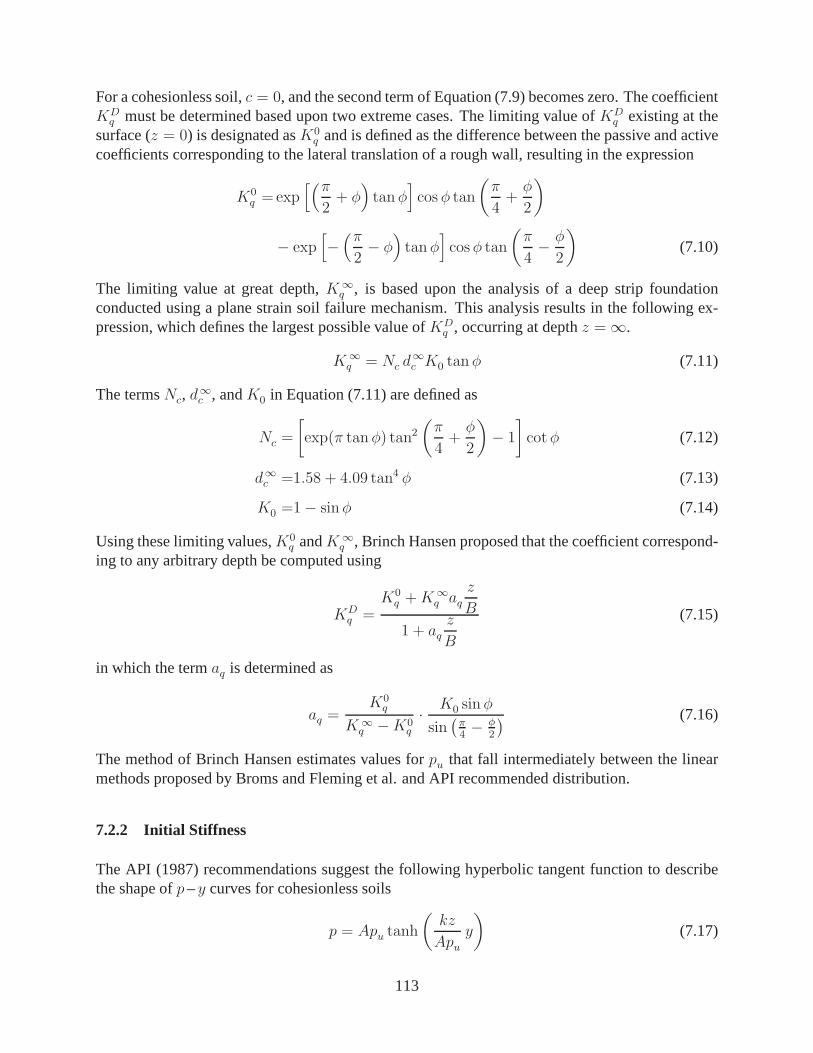
For a cohesionless soil,c = 0, and the second term of Equation (7.9) becomes zero. The coefficientKD

q must be determined based upon two extreme cases. The limiting value ofKDq existing at the

surface (z = 0) is designated asK0q and is defined as the difference between the passive and active

coefficients corresponding to the lateral translation of a rough wall, resulting in the expression

K0q =exp

[(π

2+ φ

)

tanφ]

cos φ tan

(

π

4+φ

2

)

− exp[

−(π

2− φ

)

tanφ]

cosφ tan

(

π

4− φ

2

)

(7.10)

The limiting value at great depth,K∞

q , is based upon the analysis of a deep strip foundationconducted using a plane strain soil failure mechanism. Thisanalysis results in the following ex-pression, which defines the largest possible value ofKD

q , occurring at depthz = ∞.

K∞

q = Nc d∞

c K0 tanφ (7.11)

The termsNc, d∞

c , andK0 in Equation (7.11) are defined as

Nc =

[

exp(π tanφ) tan2(

π

4+φ

2

)

− 1

]

cotφ (7.12)

d∞

c =1.58 + 4.09 tan4 φ (7.13)

K0 =1− sinφ (7.14)

Using these limiting values,K0q andK∞

q , Brinch Hansen proposed that the coefficient correspond-ing to any arbitrary depth be computed using

KDq =

K0q +K∞

q aqz

B

1 + aqz

B

(7.15)

in which the termaq is determined as

aq =K0

q

K∞

q −K0q

· K0 sinφ

sin(

π4− φ

2

) (7.16)

The method of Brinch Hansen estimates values forpu that fall intermediately between the linearmethods proposed by Broms and Fleming et al. and API recommended distribution.

7.2.2 Initial Stiffness

The API (1987) recommendations suggest the following hyperbolic tangent function to describethe shape ofp –y curves for cohesionless soils

p = Apu tanh

(

kz

Apuy

)

(7.17)

113

in whichk is the coefficient of subgrade reaction,A is a coefficient based on empirical correlationsto account for the type of loading (i.e., cyclic or static), and the other terms are as previouslydefined. Evaluating the derivative of Equation (7.17) with respect toy at the pointy = 0 leads to adefinition of the initial stiffness askT = kz.

The API recommends values of the coefficient of subgrade reaction, k, which are representativeof sands both above and below the water table. Figure 7.2 shows the representative coefficient ofsubgrade reaction values for each case as functions of relative density and internal friction angle.As shown, the coefficient of subgrade reaction increases nonlinearly as the shear strength of thesoil increases (as represented by increasing relative density or friction angle).

Figure 7.2 Recommended coefficient of subgrade reaction after API (1987). The conversionfrom units of lb/in 3 is obtained through multiplication with a factor of 271.45 toobtain units of kN/m3.

It is somewhat well known, and is shown in this report, that the linear distribution of initial stiff-ness recommended by the API does not represent the actual initial soil response well. Theserecommendations are based on lateral load tests, where the near-surface response is captured well.Extrapolation of this near-surface behavior to all depths leads to significant overestimation of theinitial stiffness at increased depth. Recognizing that theelastic modulus of sand is roughly pro-portional to the square root of confining pressure, Boulanger et al. (2003) propose an approximatecorrection for the API subgrade reaction modulus. The corrected modulus,k∗, is computed as

k∗ = cσkAPI (7.18)

114

wherekAPI is the API subgrade modulus from Figure 7.2, and the termcσ accounts for variation invertical effective stress,σ′

v, as

cσ =

√

σ′

ref

σ′

v

(7.19)

in which σ′

ref is a reference stress taken to be 50 kPa. Using this correction procedure, the initialstiffness distribution,kT = k∗z, is parabolic with depth.

7.3 COMPARISON OF COMPUTED AND PREDICTED p –y CURVES

Soil response curves computed from 3D FE analyses are used toinvestigate the applicability ofp –y curves defined using the predictive methods cited above. Thedistributions ofpu andkT along thelength of the pile obtained from the 3D model are compared to those recommended by the predic-tive methods to evaluate the validity of each respective method. Because the considered predictivemethods have no inherent ability for the inclusion of a liquefied layer, all of the comparisons madein this section are for a homogenous soil profile.

7.3.1 Comparison of Ultimate Lateral Resistance

Figure 7.3 shows computedpu distributions for three pile diameters at left and computedkT distri-butions at right. Plotted with the computedpu distributions are corresponding distributions for thepredictive methods discussed previously. These estimateddistributions ofpu are determined usingthe appropriate pile diameter and depths for each case as well as a soil unit weightγ = 17 kN/m3

and friction angleφ = 36◦, values that correspond to the the soil constitutive model in the FEanalyses.

All of the pu distributions, both computed and estimated, show an increase in resistance with depth;however, the way in whichpu increases differs across the methods and the shape of the computedpu distribution does not directly correlate to any of the considered predictive methods. At shallowdepths, there is a fair amount of agreement for all methods. This similarity occurs from the surfaceto a depth of approximately two pile diameters. Beyond this depth, the distributions begin todiverge.

The computed and predictedpu distributions display a diameter dependence. As pile diameterincreases, the corresponding value ofpu also increases. A larger zone of soil is affected by a largerpile, and consequently, more resistance is provided prior to the yield of this zone. This effectbecomes more pronounced with increasing depth. As depth andconfining pressure increase, theshear strength of the soil also increases, leading to a larger ultimate lateral resistance.

In order to evaluate the applicability of the computedpu distributions, it is important to considerhow well the fitted curve parameters represent the recorded data. Figure 7.4 shows computedp –y curves at five separate depths for a 2.5-m-diameter pile. Near the ground surface the ultimateresistance of the soil appears to have been activated and is appropriately reflected in the fittedparameters. As depth increases, it can no longer be assumed that the ultimate resistance has been

115

0 2 4 6 8 10 12x 10

4

−50

−40

−30

−20

−10

0


dept

h (m

)

API (1987)Broms (1964)Fleming et al. (1985)Brinch Hansen (1961)3D FEA 2.5 m Pile

0 2 4 6 8x 10

4

−50

−40

−30

−20

−10

0


dept

h (m

)

API (1987)3D FEA 2.5 m Pile

0 1 2 3x 10

4

−25

−20

−15

−10

−5

0


dept

h (m

)


0 1 2 3 4 5 6x 10

4

−25

−20

−15

−10

−5

0


dept

h (m

)


0 2000 4000 6000

−12

−10

−8

−6

−4

−2

0


dept

h (m

)


0 1 2 3 4x 10

4

−12

−10

−8

−6

−4

−2

0


dept

h (m

)


Figure 7.3 Distributions of ultimate lateral resistance and initial stiffness for each of thethree template pile designs as compared to commonly referenced distributions.

116

0 0.1 0.2 0.3 0.4 0.5 0.60

500

1000

1500

2000

2500

3000

3500

Horizontal displacement (m)

Hor

izon

tal f

orce

/leng

th (

kN/m

)

z = 0.625 mz = 1.875 mz = 3.125 mz = 4.375 mz = 5.625 m

Figure 7.4 Comparison of computedp –y data with fitted hyperbolic tangent curves for a2.5-m-diameter pile.

achieved. The fitted curves appear to underestimate the ultimate resistance with increasing depth,and the degree to whichpu is underestimated tends to increase with depth.

Figure 7.5, which shows the distribution of stress in the direction of pile motion at the ultimatedisplacement of the pile, further supports this observation. As shown, the soil elements at shallowerdepths have reached a limiting value of stress during the deformation process, indicative of yieldingin the soil, while the deep elements continue to gain stress,indicating that these elements have notyet experienced failure, nor activated an ultimate resistance.

The observation that the deeper curves do not display results indicating failure of the soil makessense in the context of the Drucker-Prager soil model. The confining pressure increases with depth,and an increase in confining pressure leads to an increased yield strength in the soil model. Thelimitations of the current model are such that it is not possible to push the pile far enough to suf-ficiently activate the ultimate resistance at increased depths without suffering mesh distortion andfailure of the simulation. Moreover, the small strain/deformation assumption already reaches itslimits under the considered deformations. The region over which there is confidence in the ultimatelateral resistance distributions corresponds to the depths at which the FE analysis results are similarto the estimatedpu distributions. This observation identifies the need for further resolution in thefinite element models at shallow depths. To accomplish this,near-surface models are generatedand analyzed. The results are presented and discussed in thenext section.

117

Figure 7.5 Distribution of stress in the direction of loading at full lateral displacement of a0.61-m-diameter pile in the rigid pile kinematic case.

7.3.2 Comparison of Initial Stiffness

The kT distributions obtained from 3D FE analysis vary significantly from the linear variationsuggested by the API. In Figure 7.3, the linear stiffness shown is based on a subgrade modulusfrom Figure 7.2 for an internal friction angleφ = 36◦. At any particular depth, the resulting linearkT distribution is larger in magnitude than the computed distributions. This is especially true belowthe near-surface zone.

The computed initial stiffness distributions show an expected magnitude increase with increasingdepth, however, the rate of increase is not constant over thelength of the pile. As shown in Fig-ure 7.3, thekT distributions computed from 3D FE analysis display two distinct linearly-increasingzones. The stiffness at shallow depths is significantly lessthan those at depth, though the rate ofincrease in this near-surface zone is greater. As depth increases beyond this initial zone, the rateat which the stiffness increase begins to lessen, eventually reaching a constant level marked by thesecond zone of linear increase.

The two linear zones displayed by the computedkT distributions do not correlate well with theAPI recommendations. There is a diameter dependence shown in the near-surface behavior thatis not captured at all by the APIkT distribution. For further comparison, approximate valuesofsubgrade modulus implied by the slope of the computedkT distributions are used. In the near-surface zone, the approximate subgrade moduli for each pileare summarized in Table 7.1. Takenin the context of Figure 7.2, these values correspond to lower internal friction angles than thatused in the 3D simulations. The subgrade modulus suggested at increased depths has a magnitudeof approximately1000 kN/m3, which is less than half of the lowest value ofk recommended inFigure 7.2.

The two zones of differing response observed in the distributions of initial stiffness computed from

118

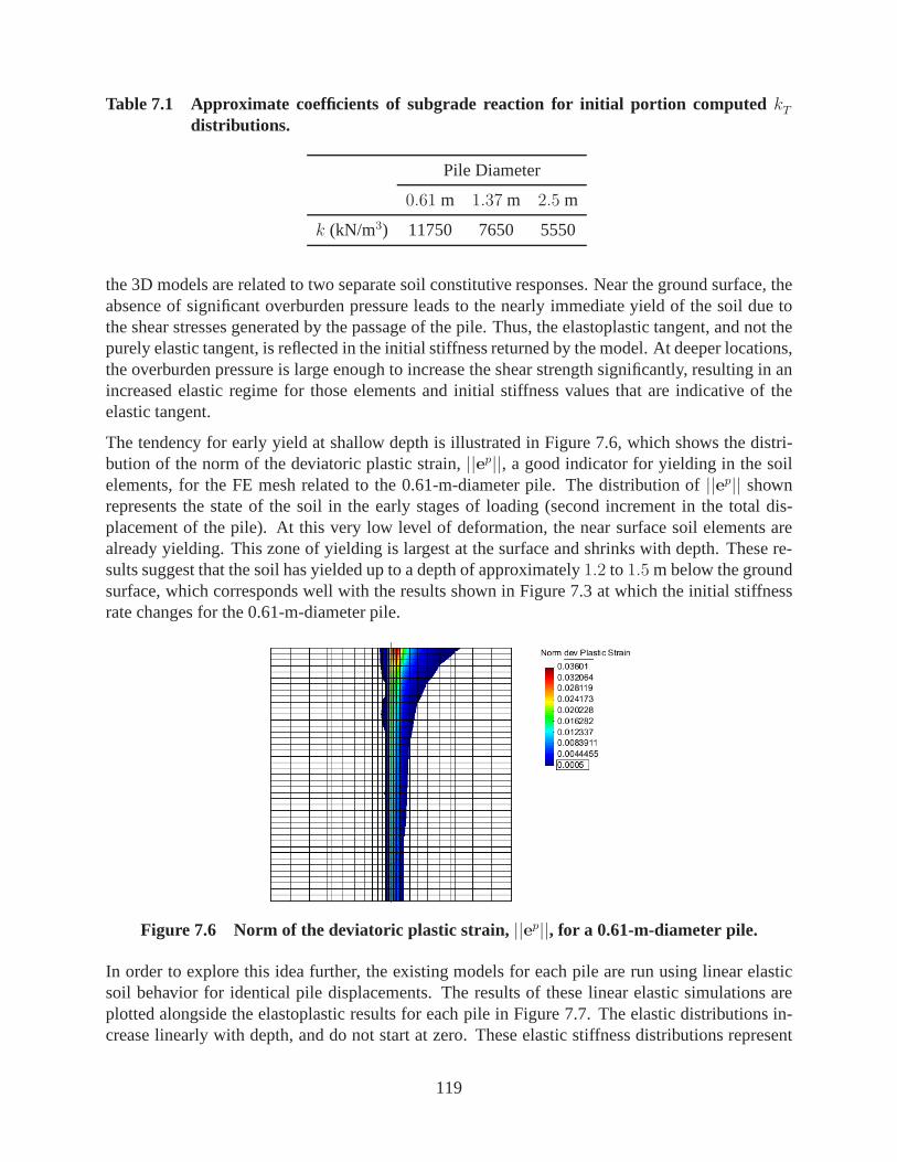
Table 7.1 Approximate coefficients of subgrade reaction forinitial portion computed kTdistributions.

Pile Diameter

0.61 m 1.37 m 2.5 m

k (kN/m3) 11750 7650 5550

the 3D models are related to two separate soil constitutive responses. Near the ground surface, theabsence of significant overburden pressure leads to the nearly immediate yield of the soil due tothe shear stresses generated by the passage of the pile. Thus, the elastoplastic tangent, and not thepurely elastic tangent, is reflected in the initial stiffness returned by the model. At deeper locations,the overburden pressure is large enough to increase the shear strength significantly, resulting in anincreased elastic regime for those elements and initial stiffness values that are indicative of theelastic tangent.

The tendency for early yield at shallow depth is illustratedin Figure 7.6, which shows the distri-bution of the norm of the deviatoric plastic strain,||ep||, a good indicator for yielding in the soilelements, for the FE mesh related to the 0.61-m-diameter pile. The distribution of||ep|| shownrepresents the state of the soil in the early stages of loading (second increment in the total dis-placement of the pile). At this very low level of deformation, the near surface soil elements arealready yielding. This zone of yielding is largest at the surface and shrinks with depth. These re-sults suggest that the soil has yielded up to a depth of approximately1.2 to 1.5 m below the groundsurface, which corresponds well with the results shown in Figure 7.3 at which the initial stiffnessrate changes for the 0.61-m-diameter pile.

Figure 7.6 Norm of the deviatoric plastic strain,||ep||, for a 0.61-m-diameter pile.

In order to explore this idea further, the existing models for each pile are run using linear elasticsoil behavior for identical pile displacements. The results of these linear elastic simulations areplotted alongside the elastoplastic results for each pile in Figure 7.7. The elastic distributions in-crease linearly with depth, and do not start at zero. These elastic stiffness distributions represent

119

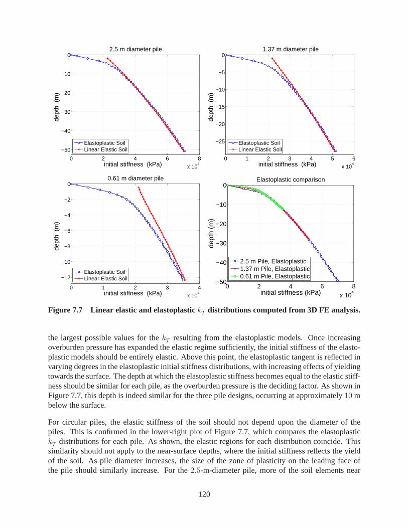
0 2 4 6 8

x 104

−50

−40

−30

−20

−10

0


dept

h (

m)

2.5 m Pile

Elastoplastic SoilLinear Elastic Soil

0 1 2 3 4

x 104

−12

−10

−8

−6

−4

−2

0


dept

h (

m)

0.6096 m Pile


0 2 4 6 8x 10

4

−50

−40

−30

−20

−10

0


dept

h (m

)

All three pile diameters

2.5 m Pile, Elastoplastic1.37 m Pile, Elastoplastic0.61 m Pile, Elastoplastic

0 1 2 3 4 5 6

x 104

−25

−20

−15

−10

−5

0


dept

h (

m)

1.3716 m Pile


2.5 m diameter pile 1.37 m diameter pile

0.61 m diameter pile Elastoplastic comparison

Figure 7.7 Linear elastic and elastoplastickT distributions computed from 3D FE analysis.

the largest possible values for thekT resulting from the elastoplastic models. Once increasingoverburden pressure has expanded the elastic regime sufficiently, the initial stiffness of the elasto-plastic models should be entirely elastic. Above this point, the elastoplastic tangent is reflected invarying degrees in the elastoplastic initial stiffness distributions, with increasing effects of yieldingtowards the surface. The depth at which the elastoplastic stiffness becomes equal to the elastic stiff-ness should be similar for each pile, as the overburden pressure is the deciding factor. As shown inFigure 7.7, this depth is indeed similar for the three pile designs, occurring at approximately10 mbelow the surface.

For circular piles, the elastic stiffness of the soil shouldnot depend upon the diameter of thepiles. This is confirmed in the lower-right plot of Figure 7.7, which compares the elastoplastickT distributions for each pile. As shown, the elastic regions for each distribution coincide. Thissimilarity should not apply to the near-surface depths, where the initial stiffness reflects the yieldof the soil. As pile diameter increases, the size of the zone of plasticity on the leading face ofthe pile should similarly increase. For the2.5-m-diameter pile, more of the soil elements near

120

0 0.1 0.2 0.30

500

1000

1500

2000

displacement y (m)

forc

e de

nsity

p (

kN/m

)


0 0.1 0.2 0.30

500

1000

1500

2000

displacement y (m)

forc

e de

nsity

p (

kN/m

)


0 0.1 0.2 0.30

2000

4000

6000

8000

10000

12000

displacement y (m)

forc

e de

nsity

p (

kN/m

)


0 0.1 0.2 0.30

2000

4000

6000

8000

10000

12000

displacement y (m)

forc

e de

nsity

p (

kN/m

)


API (1987)Fitted tanh curveOpenSees data

displacement y (m)

1.0 m below surface

9.9 m below surface 14.7 m below surface

2.4 m below surface

forc

e de

nsity

p (

kN/m

)

0

0

4000

12000

8000

1000

2000

0 0.1 0.2 0 0.1 0.20.3 0.3

Figure 7.8 Computed and API recommendedp –y curves for a 1.37-m-diameter pile.

the surface are yielding than for the smaller piles, therefore, the initial stiffness returned for thislarger pile is generally lower than those corresponding to the smaller piles near the surface. This isreflected in the extracted curves shown in Figure 7.7 and in the approximate near-surface subgrademodulus values summarized in Table 7.1. The stiffness at a given depth increases with decreasingpile diameter in this plastic zone.

The observation that the computedkT distributions for the three pile diameters are similar at depthbut differ near the ground surface leads to the desire to obtain a higher degree of resolution onthe near-surface areas. A series of10 m deep meshes are generated, one for each pile design, andanalyzed using the same pile deformations. These results offer a means of validating observationsmade, as well as a closer look at the near-surface effects.

7.3.3 Comparison ofp –y Curves

Figure 7.8 shows representative computedp –y data and fitted hyperbolic tangent curves obtainedfor a 1.37-m-diameter pile. The API 1987 recommendedp –y curves are shown for comparison.As is expected based upon the observed differences inkT andpu between the computed and APIcurves, the two sets of curves are comparable at shallow depths while differing substantially atgreater depths. For analysis of top-loaded piles, these differences are relatively inconsequential;however, for analysis of a lateral spreading deformation, where large pile deformation can occur atdepth, the problems created by these differences become apparent.

7.4 NEAR-SURFACE MODELS

In an effort to gain better insight in the results near the surface, a series of new meshes are generatedthat only consider the first 10 m below the surface. Modeling only the upper 10 m allows theanalyses to focus on the zone of pronounced plasticity in thesoil. Due to lessons learned about

121

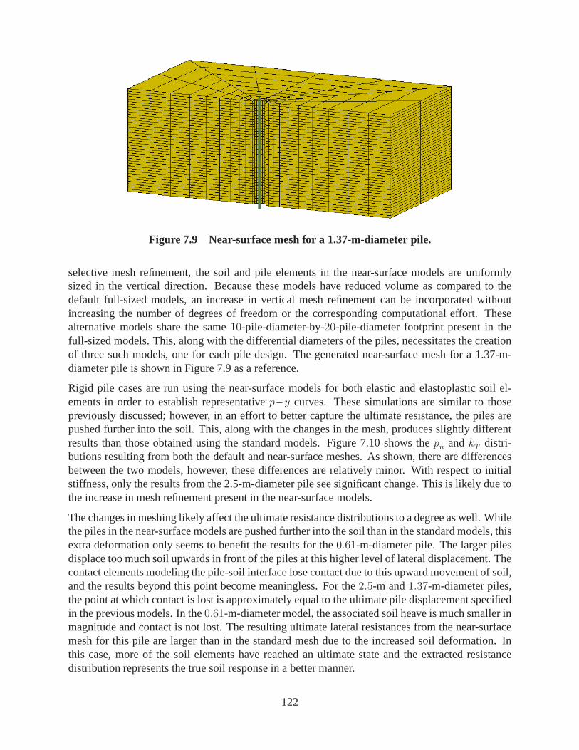
Figure 7.9 Near-surface mesh for a 1.37-m-diameter pile.

selective mesh refinement, the soil and pile elements in the near-surface models are uniformlysized in the vertical direction. Because these models have reduced volume as compared to thedefault full-sized models, an increase in vertical mesh refinement can be incorporated withoutincreasing the number of degrees of freedom or the corresponding computational effort. Thesealternative models share the same10-pile-diameter-by-20-pile-diameter footprint present in thefull-sized models. This, along with the differential diameters of the piles, necessitates the creationof three such models, one for each pile design. The generatednear-surface mesh for a 1.37-m-diameter pile is shown in Figure 7.9 as a reference.

Rigid pile cases are run using the near-surface models for both elastic and elastoplastic soil el-ements in order to establish representativep –y curves. These simulations are similar to thosepreviously discussed; however, in an effort to better capture the ultimate resistance, the piles arepushed further into the soil. This, along with the changes inthe mesh, produces slightly differentresults than those obtained using the standard models. Figure 7.10 shows thepu andkT distri-butions resulting from both the default and near-surface meshes. As shown, there are differencesbetween the two models, however, these differences are relatively minor. With respect to initialstiffness, only the results from the 2.5-m-diameter pile see significant change. This is likely due tothe increase in mesh refinement present in the near-surface models.

The changes in meshing likely affect the ultimate resistance distributions to a degree as well. Whilethe piles in the near-surface models are pushed further intothe soil than in the standard models, thisextra deformation only seems to benefit the results for the0.61-m-diameter pile. The larger pilesdisplace too much soil upwards in front of the piles at this higher level of lateral displacement. Thecontact elements modeling the pile-soil interface lose contact due to this upward movement of soil,and the results beyond this point become meaningless. For the 2.5-m and1.37-m-diameter piles,the point at which contact is lost is approximately equal to the ultimate pile displacement specifiedin the previous models. In the0.61-m-diameter model, the associated soil heave is much smaller inmagnitude and contact is not lost. The resulting ultimate lateral resistances from the near-surfacemesh for this pile are larger than in the standard mesh due to the increased soil deformation. Inthis case, more of the soil elements have reached an ultimatestate and the extracted resistancedistribution represents the true soil response in a better manner.

122

0 1 2 3 4

x 104

−10

−8

−6

−4

−2

0


dept

h (

m)

2.5 m Pile

Near−Surface MeshDefault Mesh

0 1 2 3 4

x 104

−10

−8

−6

−4

−2

0


dept

h (

m)

1.3716 m Pile


0 1 2 3 4

x 104

−10

−8

−6

−4

−2

0


dept

h (

m)

0.6096 m Pile


0 1000 2000 3000 4000 5000 6000 7000−10

−8

−6

−4

−2

0


dept

h (

m)

2.5 m Pile


0 1000 2000 3000 4000 5000−10

−8

−6

−4

−2

0


dept

h (

m)

1.3716 m Pile


0 1000 2000 3000 4000−10

−8

−6

−4

−2

0


dept

h (

m)

0.6096 m Pile


2.5 m diameter pile

1.37 m diameter pile

0.61 m diameter pile

Figure 7.10 Comparisonpu and kT distributions for default and near-surface meshes overthe first 10 m below the ground surface.

123

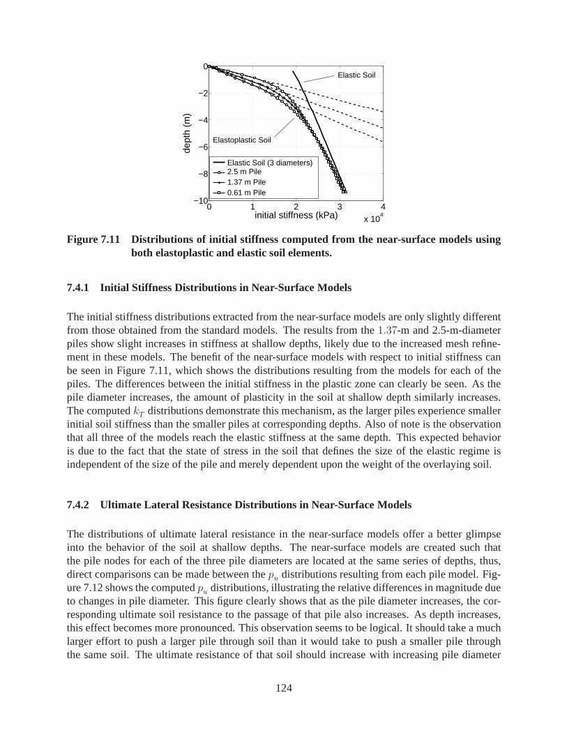
0 1 2 3 4x 10

4

−10

−8

−6

−4

−2

0


dept

h (m

)

Elastic Soil

Elastoplastic Soil

Elastic Soil (3 diameters)2.5 m Pile

0.61 m Pile1.37 m Pile

Figure 7.11 Distributions of initial stiffness computed from the near-surface models usingboth elastoplastic and elastic soil elements.

7.4.1 Initial Stiffness Distributions in Near-Surface Models

The initial stiffness distributions extracted from the near-surface models are only slightly differentfrom those obtained from the standard models. The results from the1.37-m and 2.5-m-diameterpiles show slight increases in stiffness at shallow depths,likely due to the increased mesh refine-ment in these models. The benefit of the near-surface models with respect to initial stiffness canbe seen in Figure 7.11, which shows the distributions resulting from the models for each of thepiles. The differences between the initial stiffness in theplastic zone can clearly be seen. As thepile diameter increases, the amount of plasticity in the soil at shallow depth similarly increases.The computedkT distributions demonstrate this mechanism, as the larger piles experience smallerinitial soil stiffness than the smaller piles at corresponding depths. Also of note is the observationthat all three of the models reach the elastic stiffness at the same depth. This expected behavioris due to the fact that the state of stress in the soil that defines the size of the elastic regime isindependent of the size of the pile and merely dependent uponthe weight of the overlaying soil.

7.4.2 Ultimate Lateral Resistance Distributions in Near-Surface Models

The distributions of ultimate lateral resistance in the near-surface models offer a better glimpseinto the behavior of the soil at shallow depths. The near-surface models are created such thatthe pile nodes for each of the three pile diameters are located at the same series of depths, thus,direct comparisons can be made between thepu distributions resulting from each pile model. Fig-ure 7.12 shows the computedpu distributions, illustrating the relative differences in magnitude dueto changes in pile diameter. This figure clearly shows that asthe pile diameter increases, the cor-responding ultimate soil resistance to the passage of that pile also increases. As depth increases,this effect becomes more pronounced. This observation seems to be logical. It should take a muchlarger effort to push a larger pile through soil than it wouldtake to push a smaller pile throughthe same soil. The ultimate resistance of that soil should increase with increasing pile diameter

124

0 2000 4000 6000 8000−10

−8

−6

−4

−2

0


dept

h (m

)

2.5 m Pile1.3716 m Pile0.6096 m Pile

2.5 m Pile1.37 m Pile0.61 m Pile

Figure 7.12 Computedpu distributions for near-surface models.

and with increasing overburden pressure, exactly as observed from the results of the near-surfacemodels.

The ultimate resistance of the soil does not become fully activated at advanced depths in the defaultmesh FE analysis. In an effort to gain a better estimate of this value with depth, the piles are pushedfurther into the soil in the near-surface models. As previously discussed, loss of contact betweenthe larger piles and the soil due to a meshing issue renders this extra deformation meaninglessfor those models, however, the 0.61-m-diameter pile sees increased values ofpu over the resultsobtained from the standard model because of the extended lateral pile displacement. Though theresults from the larger pile models do not see the benefits of the extra push, there is an increase inthe number of adequately estimated points on thepu distribution curves due to the decreased meshsize in the near-surface models as compared to the full-sized (default) counterparts.

7.5 PLANE STRAIN MODELS

With the current mesh and element formulations primarily used in this research, it seems unlikelythat the models will be able to capture the true ultimate lateral resistance at all depths along thelength of the pile. To establish the maximum attainable value ofpu at a given depth, a plane strainsoil model is created. This model also allows a direct comparison to the estimatedpu distributionsusing the methods proposed by Brinch Hansen (1961) and API (1987). These two methods as-sumed a plane strain failure mechanism at depth, and the plane strain FE model allows insight intohow close conditions in the default 3D model are to plane strain at increased depth.

As this is only a validation exercise, only a single plane strain model is created. This modelconsiders the 2.5-m-diameter pile embedded in a soil continuum. The plane strain mesh shares afootprint with the corresponding standard mesh; however, the plane strain soil mesh is only oneelement thick in the vertical direction. The pile is reducedin length down to two elements withthe middle pile node located at the center of the layer of soilelements. In order to compare the

125

0 0.5 1 1.5 2 2.5 3

x 104

−50

−40

−30

−20

−10

0


dept

h (

m)

2.5 m Pile

Plane strain modelDefault model

0 1 2 3 4 5 6 7

x 104

−50

−40

−30

−20

−10

0


dept

h (

m)

2.5 m Pile

Plane strain modelDefault model

Figure 7.13 Comparison parameter distributions for default and plane strain FE models.

results of the plane strain model with other results, a method of simulating depth is devised thatemploys the surface load element developed for use in OpenSees during this research. A detaileddiscussion of these elements is provided in Section 2.5.

In order to obtain a distribution of results with depth at a minimum of modeling effort, a seriesof five depths is established. These depths are selected suchthat the resulting data provides ageneral sense of thep –y curve parameter distributions over the full length of the pile. Appropriateoverburden pressures corresponding to each of these depthsare applied to the meshes via thesurface load elements in order to determine the resulting displacements of the upper surface ofthe soil elements. When running the plane strain model, the upper nodes of the soil layer areslowly moved via displacement control through these recorded displacements, creating a depth-appropriate initial stress state in the soil elements, and then held fixed in the vertical direction asthe pile is pushed into the soil layer. In this manner, the response of the soil for each of the selecteddepths is established for the plane strain condition.

In the plane strain model, there is no free surface. The earlyplasticity observed in the regular meshat shallow depths should not occur. It is expected that the initial stiffness distribution obtainedfrom the plane strain model should exceed that obtained fromthe standard mesh at shallow depths.At increased depths, the values ofkT obtained from either model should be approximately equal.Assuming the conditions in the default mesh at greater depths are nearly plane strain, the increasein elastic stiffness from the plane strain condition shouldnot be significant.

The ultimate lateral resistances obtained from the plane strain model should be larger than thoseextracted from the standard model at corresponding depths,especially near the surface where theassumption of a plane strain failure mode is poor. The plane strain condition allows significantlylarger confining pressures to develop in the soil elements, leading to a corresponding increase instrength. For this reason, the ultimate resistances from the plane strain model should represent thelargest possible resistances that the soil can provide for the lateral displacement of a pile.

Figure 7.13 shows the distributions ofpu andkT obtained from the plane strain model. As ex-pected, near the surface, thekT distribution is in excess of that obtained from the default model; at

126

0 2 4 6 8 10 12

x 104

−50

−45

−40

−35

−30

−25

−20

−15

−10

−5

0


dept

h (m

)

API (1987)Broms (1964)Fleming et al. (1985)Brinch Hansen (1961)Plane strain FEA

Figure 7.14 Comparison of estimatedpu distributions with corresponding results fromplane strain model for a 2.5-m-diameter pile.

depth the distributions are nearly identical. Thepu distribution obtained from the plane strain casealso displays the expected behavior. At each depth, the value ofpu resulting from the plane straincondition is greater in magnitude than the corresponding value from the default mesh case. Thedegree to which these values are exceeded decreases with depth. At a depth of1 m, where the de-fault models have shown that the plane strain assumption is not applicable, the ultimate resistancein the plane strain model is approximately ten times larger than the previous result, while at50 mbelow the surface, the plane strain resistance is about1.3 times larger.

Figure 7.14 shows estimated distributions for four predictive methods (Broms, 1964; Fleming et al.,1985; Brinch Hansen, 1961; API, 1987) alongside the distribution of pu obtained from the planestrain FE analysis. As shown, the computed values ofpu at depth are significantly less than thosepredicted using the API method and are more similar to those predicted by the method of Fleminget al. (1985) or Brinch Hansen (1961).

7.6 SUMMARY

In current practice, thep –y method, which models the soil-pile system as a beam on a nonlinearWinkler foundation, is commonly employed in the analysis ofpiles subject to lateral loads. Someconventional methods that may be employed in the definition of parameters appropriate for use inp –y curves have been compared. It is observed that there are significant differences in the distri-butions of ultimate lateral resistance estimated by these methods at depths beyond the first few pilediameters below the surface. It is also observed that the distributions ofpu computed from the 3DFE models generally do not correlate well in their form with any of the predictive methods, though

127

the magnitudes of the resistances are relatively similar tothe softer of the considered predictivemethods. The prevalent distribution of initial stiffness recommended for use inp –y curves is en-tirely linear and appears to be more appropriately applied to near-surface depths where the effectsof early soil yield are observed. At increased depth, the full elastic stiffness of the soil is initiallyactive. These values are significantly less than those suggested by conventional methods.

The method for obtaining ultimate resistances recommendedby the API (1987) is one of the mostcommonly employed methods in the construction ofp –y curves for cohesionless soil. This methodis based essentially upon a single series of field tests in which the piles are loaded at or above theground surface. As discussed in Section 6.5, the pile kinematics greatly influence the recordedsoil response, suggesting that results obtained from a top-pushover kinematic are not necessarilyapplicable to alternative load cases. Reese and Van Impe (2001) mention that there is more con-fidence in the form of the predicted results than in the magnitude, which appears to be a fairlyvalid conclusion as the plane strain FE analysis results provide further evidence that the predictedmagnitudes may be excessive.

It is important to note that in the analysis of the top-pushover kinematic, an overestimation of theinitial stiffness and ultimate lateral resistance at depthis relatively harmless. In places where theparameter distributions are excessively large, the piles are not undergoing deflections due to thekinematics of the loading. However, in the lateral spreading case, large pile deformations mayoccur in the areas wherekT andpu are too large. In simplified analysis of piles subject to lateralspreading, careful selection ofp –y curve parameters is essential.

128

8 Influence of Liquefied Layer on the SoilResponse

8.1 INTRODUCTION

In liquefaction-induced lateral spreading, after the onset of liquefaction, the shear strength of theaffected soil is reduced significantly. The unliquefied soilnear the layer interface is now ableto squeeze into the softer layer near the pile during the application of a lateral load, effectivelyreducing the available lateral capacity and stiffness of the unliquefied soil near the liquefied layer.

Similar behavior occurs for laterally-loaded piles embedded in layered soil profiles in which astrength differential exists between two adjacent layers,e.g., a soft clay layer located between twolayers of dense sand. Yang and Jeremic (2005) demonstrated this behavior using 3D FE analysis,and with respect to BNWF analysis of piles, Georgiadis (1983) developed a method to modifyp –ycurves to account for differential layers. In a BNWF analysis of a pile subject to lateral spreading,thep –y curves should be similarly modified to account for the presence of the liquefied soil layer.

The effect of a liquefied layer on the response of the adjacentunliquefied soil layers is evaluatedthrough comparisons between the results of 3D FE analysis both with and without a liquefied layer.Through the use of overburden pressure applied to the surface of the models, the effect of varyinglevels of vertical stress at the liquefied interface is also investigated. These initial observationsidentify the need for a more comprehensive approach to the problem.

A series of new FE meshes are generated and used to compute representativep –y curves for aseries of soil profiles in which the vertical location and thickness of the liquefied layer are varied.It is determined that the reduction in thep –y curve parameters of initial stiffness and ultimatelateral resistance is greatest at the layer interface and decays exponentially with increasing distancefrom the liquefied layer. A simplified procedure is developedto determine appropriate reductionsin initial stiffness and ultimate lateral resistance forp –y curves representing the unliquefied soilnear the liquefied interface.

8.2 INITIAL OBSERVATIONS

The FE mesh discussed in Chapter 2 is used to evaluate the effect of a liquefied layer on the initialstiffness and ultimate lateral resistance of the unliquefied soil. In this model, the liquefied layer is

129


dept

h (

m)

0 1000 2000 3000 4000 5000 6000 7000

−25

−20

−15

−10

−5

0

Homogenous ProfileLiquefied Layer Included


dept

h (

m)

0 0.5 1 1.5 2 2.5 3

x 104

−25

−20

−15

−10

−5

0

Homogenous ProfileLiquefied Layer Included

Figure 8.1 Distributions of pu and kT for homogenous and liquefied soil profiles for a 1.37-m-diameter pile.

located at a depth of 10 pile diameters below the ground surface and has a thickness of one pilediameter. This soil profile is not ideal for fully characterizing the influence of the liquefied layerfor a general case; however, it is used in order to determine the important factors which affect thisbehavior. To this purpose,p –y curves are computed for homogenous soil profiles and profileswith a liquefied middle layer. The resulting curves are compared with respect to ultimate lateralresistance,pu, and initial stiffness,kT . Increasing depth to the liquefied layer is simulated throughthe application of overburden stresses to the ground surface of the model. This creates a stress stateat the liquefied interface that corresponds to a deeper liquefied layer location.

Figure 8.1 presents a comparison of thepu andkT distributions resulting from homogenous andliquefied cases for a 1.37-m-diameter pile with no additional overburden pressure. These resultsare typical of all the considered cases, and have been smoothed to account for variations in meshsize using the procedure discussed in Section 6.6. As shown,the effects of the liquefied layer onthe adjacent unliquefied layers are more evident in the distribution ofpu than that ofkT . The curvedata obtained from within the liquefied layer is not always ofa form that lends itself well to ahyperbolic tangent curve fit. For this reason, values ofpu cannot be computed at some of thesenodes. The general trends are still apparent, however, and that is the more important consideration.

The portions of thepu andkT distributions in both the upper and lower solid layers are affectedby the presence of the liquefied middle layer. The observed reductions in these parameters lessenin magnitude with increasing distance from the liquefied interface. Near the top and bottom ofthe soil profile, the homogenous and liquefied cases display nearly identical results. The observedreductions in ultimate resistance and initial stiffness are due to a similar behavior as that observedand discussed at shallow depths in Section 7.4. As the pile ispushed laterally into the soil profile,the soil from the solid layers is able to be pushed into the adjacent weaker layer more easily than itcan be compressed laterally. This behavior is illustrated in Figure 5.4, which shows the deformedshape of the soil elements in the vicinity of the liquefied layer. When the soil is able to expand inthis manner, it results in a decrease in the confining pressure in the areas adjacent to the liquefiedlayer and a subsequent decrease in the elastic regime for those elements. The soil in these locations

130

yielding sooner and thus cannot offer as much resistance to the passage of the pile before reachingits ultimate state.

It is of interest to evaluate the differences in effects of the liquefied layer on the two solid layers.The plots of Figure 8.1 provide a good visual comparison between the results obtained from eachsoil profile, however, it is difficult to gauge relative reductions. In order to provide a better measureof the relative differences between the homogenous and liquefied soil profiles, the ratios of the ul-timate resistance and initial stiffness in the liquefied case are taken with respect to the homogenouscase, e.g.,

pu ratio =p(liquefied)u

p(homogenous)u

(8.1)

These ratios are plotted for a 1.37-m-diameter pile in Figures 8.2 and 8.3 for five considered over-burden pressures, representing five different locations ofthe liquefiable layer. The surcharge pres-sures are based on hypothetical soil fills with vertical thicknesses of 5, 10, 15, and 20 diametersof the 1.37-m-diameter pile. This results in surcharge pressures of 117, 233, 350, and 466 kPa,respectively, for a soil unit weight ofγ = 17 kN/m3. In Figures 8.2 and 8.3 the location of theliquefied layer is indicated by the shaded region, and the presented results are typical of thoseobtained for all three piles.

The soil compacts under the applied overburden pressure andself-weight resulting in settlements.The diagrams are shown on the deformed soil body. As the applied overburden pressure increases,the zone of reduced ultimate resistance tends to decrease inthickness, meaning that a lesser extentof the solid layers are affected by the liquefied layer. This is illustrated well through comparison ofthepu ratios for all five overburden pressures at lower right in Figure 8.2. As overburden pressureincreases, corresponding to a deeper location for the liquefied layer, the reduction inpu decreases.At increased overburden pressures, there is increased shear strength in the upper and lower solidlayers, which creates a smaller plastic zone. The two layersappear to be affected approximatelyequally at all five overburden pressures. This is a significant observation given the fact that methodscommonly employed in BNWF analysis for accounting for the presence of a soft soil layer, suchas that proposed by Georgiadis (1983), only consider the effects of a soft layer on the underlayingsolid layer. The observation that both surrounding layers are affected by a weaker middle layerconfirms similar observations made by Yang and Jeremic (2005) and Petek (2006).

When the five initial stiffness ratios are shown together in the lower right plot of Figure 8.3, it isobserved that there is little difference in the reductions in initial stiffness for increasing overburdenpressures. The reduction in initial stiffness is also not nearly as widespread or as significant as theobserved reduction inpu. It appears that for a given liquefied layer thickness, the effects of thislayer on the initial response of the surrounding solid layers is relatively consistent.

131

pu ratio

dept

h (

m)

pvo

= 0 kPa

0 0.5 1 1.5 2

−25

−20

−15

−10

−5

0

pu ratio

dept

h (

m)

pvo

= 116.6 kPa

0 0.5 1 1.5 2

−25

−20

−15

−10

−5

0

pu ratio

dept

h (

m)

pvo

= 233.2 kPa

0 0.5 1 1.5 2

−25

−20

−15

−10

−5

0

pu ratio

dept

h (

m)

pvo

= 349.8 kPa

0 0.5 1 1.5 2

−25

−20

−15

−10

−5

0

pu ratio

dept

h (

m)

pvo

= 466.4 kPa

0 0.5 1 1.5 2

−25

−20

−15

−10

−5

0

pu ratio

dept

h (m

)

0.2 0.4 0.6 0.8 1 1.2−22

−20

−18

−16

−14

−12

−10

−8

−6

0 kPa116.6 kPa233.2 kPa349.8 kPa466.4 kPa

Figure 8.2 Computedpu ratios for a series of overburden pressures,pvo. The five cases arecompared at lower right.

132

kT ratio

dept

h (

m)

pvo

= 0 kPa

0 0.5 1 1.5 2

−25

−20

−15

−10

−5

0

kT ratio

dept

h (

m)

pvo

= 116.6 kPa

0 0.5 1 1.5 2

−25

−20

−15

−10

−5

0

kT ratio

dept

h (

m)

pvo

= 233.2 kPa

0 0.5 1 1.5 2

−25

−20

−15

−10

−5

0

kT ratio

dept

h (

m)

pvo

= 349.8 kPa

0 0.5 1 1.5 2

−25

−20

−15

−10

−5

0

kT ratio

dept

h (

m)

pvo

= 466.4 kPa

0 0.5 1 1.5 2

−25

−20

−15

−10

−5

0

kT ratio

dept

h (m

)

0.2 0.4 0.6 0.8 1 1.2−22

−20

−18

−16

−14

−12

−10

−8

−6

0 kPa116.6 kPa233.2 kPa349.8 kPa466.4 kPa

Figure 8.3 ComputedkT ratios for a series of overburden pressures,pvo. The five cases arecompared at lower right.

133

Pile

Unliquefied

LiquefiedLayer

Layers

Figure 8.4 Updated layered soil 3D FE mesh.

8.3 UPDATED FINITE ELEMENT MODEL

The findings of these initial studies identify the need for a detailed examination of the effects ofthe liquefied middle layer on the surrounding unliquefied soil. For this purpose, a new FE modelmust be created in which the depth and thickness of the liquefied layer are not fixed. This modeltakes into account previous findings with respect to selective mesh refinement and eliminates thediameter-dependent depth scheme used in previously discussed models. With this new model, thevertical location and depth of the liquefied layer are variedto create a series of soil profiles.

The updated model has a height of 40 m and lateral extents of 10pile diameters. Figure 8.4 showsthe undeformed configuration of the updated FE mesh. The element formulations, boundary andloading conditions, and general scheme of the model match those discussed in previous chapters.The rigid pile kinematic is used to computep –y curves from this model.

8.3.1 Considered Soil Profiles

To obtain results representative of a variety of field conditions, a set of 21 soil profiles is consideredfor each of three pile diameters (0.61 m, 1.37 m, and2.5 m). These profiles are differentiated bythe thickness of the liquefied layer,T , and the depth to the bottom of the liquefied layer,H. Theset of profiles includes four values ofT and six values ofH in order to capture the effects ofthese variables on the computedp –y curves. Table 8.1 summarizes the considered soil profiles.The symbols corresponding to each depth are used to identifyrespective cases in Figures 8.10and 8.11. Unmarked depth and thickness combinations are notconsidered.

134

8.4 CHARACTERIZING THE INFLUENCE OF THE LIQUEFIED LAYER

Figure 8.5 shows the distributions ofpu andkT for p –y curves resulting from 3D rigid pile FEanalysis with a 0.61-m-diameter pile embedded in both a homogenous soil profile and a layeredprofile having a liquefied middle layer. For simplicity, the latter profile will be referred to as theliquefied profile. These results are similar to those found during the initial analyses and presentedin Figure 8.1. The reductions inpu andkT are functions of the depth to the liquefied interface,characterized by the depth to the bottom of the liquefied layer,H, and the thickness of the liquefiedlayer,T . Similar results are obtained for 1.37-m and 2.5-m-diameter piles (not shown).

8.4.1 Reduction in Ultimate Lateral Resistance

Computedpu ratios are shown in Figures 8.6 and 8.7 for the upper and lowerunliquefied layers,respectively (the FE analysis data are represented as markers). As shown, for a constant lique-fied layer depth the reduction inpu tends to increase with increasing liquefied layer thickness, T ,though there appears to be a limit to this effect, as thepu ratios forT = 5 m andT = 10 m areessentially identical. For constantT , the reduction inpu at a given distance from the liquefiedlayer, s, decreases for increasing liquefied layer depth. The ratiosshown in Figures 8.6 and 8.7are for a single pile diameter. As pile diameter increases, the pu reduction at a given distancesincreases for a particular soil profile.

8.4.2 Reduction in Initial Stiffness

Figures 8.8 and 8.9 show computedkT ratios for the upper and lower unliquefied layers (the mark-ers are the FE analysis data). The reductions inkT have the same depth dependence observed in thepu ratios, however, changes in liquefied layer thickness only affect minor changes inkT . Signifi-cant reductions inkT are more local to the liquefied interface, especially in the lower unliquefiedlayer. The extents of the affected zone increase with increasing pile diameter. The results for a1.37-m-diameter pile are shown in Figures 8.8 and 8.9 to provide a better representation of theform of the computedkT ratios.

135

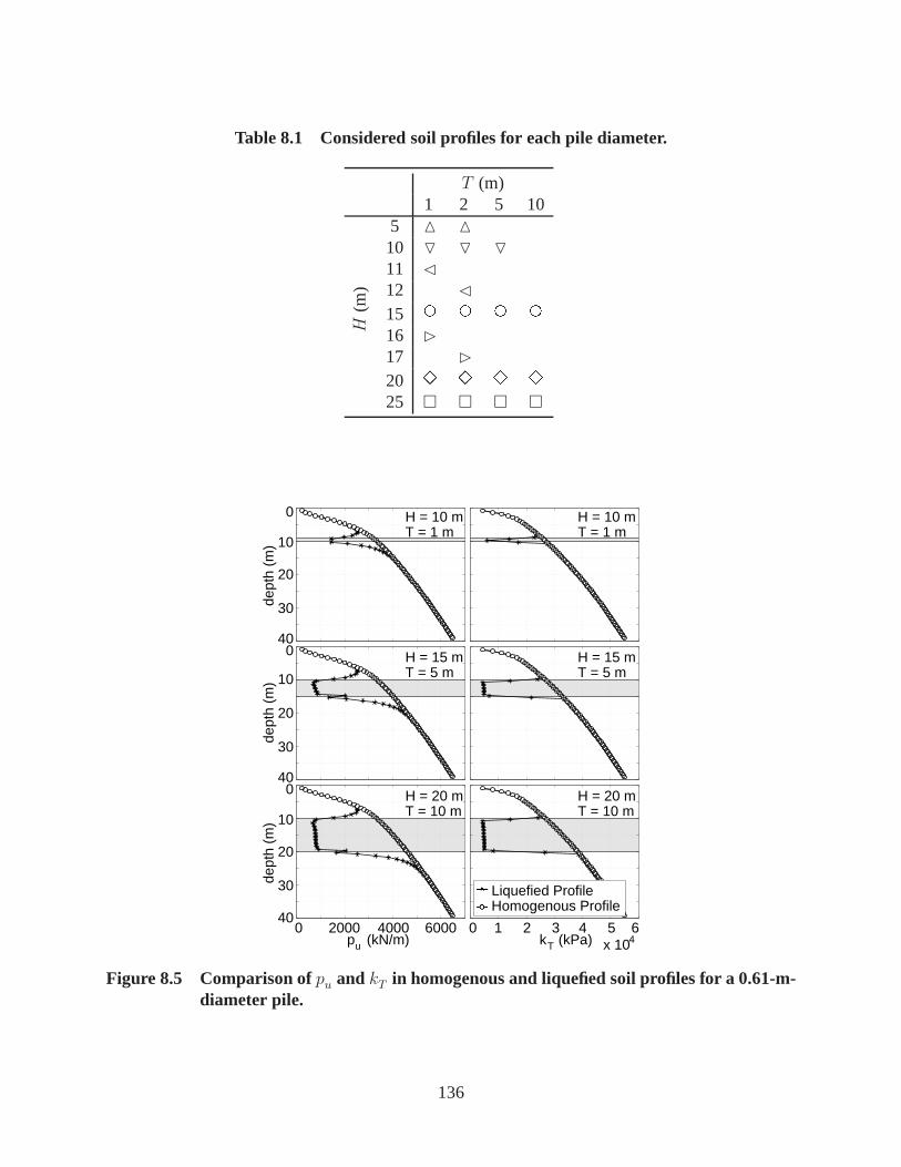
Table 8.1 Considered soil profiles for each pile diameter.

T (m)1 2 5 10

H(m

)

5 △ △

10 ▽ ▽ ▽

11 ⊳

12 ⊳

15 E E E E16 ⊲

17 ⊲

20 6 6 6 625 � � � �

T = 10 mH = 20 m

T = 10 mH = 20 m

T = 5 mH = 15 m

T = 5 mH = 15 m

T = 1 mH = 10 m

T = 1 mH = 10 m

Liquefied Profile

600040002000k (kPa)Tp (kN/m)

0 1 2 3 4 54x 106

u

040

30

20

10

0

dept

h (m

)

40

30

20

dept

h (m

) 10

040

30

20

10

0

dept

h (m

)

Homogenous Profile

Figure 8.5 Comparison ofpu and kT in homogenous and liquefied soil profiles for a 0.61-m-diameter pile.

136

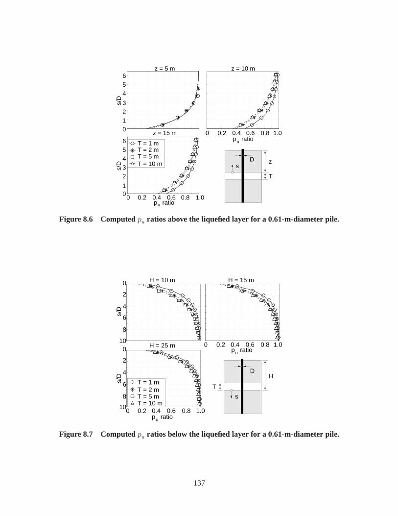
z = 10 mz = 5 m

z

T

s/D

T = 1 mT = 2 mT = 5 mT = 10 m

s/D

z = 15 m0123

456

65432

10

0 0.2 0.4 0.6 0.8 1.0p ratiou

0 0.2 0.4 0.6 0.8p ratiou

1.0

sD

Figure 8.6 Computedpu ratios above the liquefied layer for a 0.61-m-diameter pile.

6

0

6

4

2

8

10

s/D

s/D

0

2

4

8

10

H = 10 m H = 15 m

H = 25 m 0p ratio

T

s

D

0.2 0.4 0.6 0.8u

1.0

H

0 0.2 0.4 0.6 0.8 1.0p ratiou

T = 1 mT = 2 mT = 5 mT = 10 m

Figure 8.7 Computedpu ratios below the liquefied layer for a 0.61-m-diameter pile.

137

z = 10 mz = 5 m

z

T

s/D

T = 1 mT = 2 mT = 5 mT = 10 m

s/D

z = 15 m0

00 0.2 0.4 0.6 0.8 1.0

p ratiou

0 0.2 0.4 0.6 0.8p ratiou

1.0

3

2

1

3

2

1

sD

Figure 8.8 ComputedkT ratios above the liquefied layer for a 1.37-m-diameter pile.

0 0.2 0.4 0.6 0.8 1.0p ratiou

0

s/D

s/D

0

H = 25 m

H = 10 m H = 15 m

6

4

2

6

4

2

p ratio

T

s

D

0 0.2 0.4 0.6 0.8u

1.0

HT = 1 mT = 2 mT = 5 mT = 10 m

Figure 8.9 ComputedkT ratios below the liquefied layer for a 1.37-m-diameter pile.

138

8.5 REDUCTION MODEL

The reduction ratios shown in Figures 8.6 through 8.9 all share a similar functional form, suggest-ing an exponential decay model to characterize bothp –y curve parameters (McGann et al., 2010).The proposed exponential decay function

R(p,k)(s) = 1−R(p,k)0 exp

(

− s

s(p,k)c

)

(8.2)

defines a reduction factor,R, as a function of distance from the liquefied interface,s, in termsof two independent parameters,R0 andsc. The interface reduction,R0, defines the magnitude ofthe reduction at the layer interface (s = 0), and the characteristic length,sc, defines how quicklythe reduction becomes negligible. The reduction factor of Equation (8.2) is applicable to bothpu andkT distributions, and the superscripts are used to differentiate between the two, e.g.;R(p)

corresponds to a reduction factor forpu.

Using least squares, the exponential decay function in Equation (8.2) is fit with thepu andkTratio data. Examples of fitted curves are shown in Figures 8.6through 8.9 as solid or dashed lines(the markers represent points computed from individual 3D FE analysis). As shown, the chosenexponential decay function represents the data very well inboth the top and bottom layers for bothp –y curve parameters.

8.5.1 Parameter Identification

In order to establish a means to predict appropriate reductions inpu andkT for a general combi-nation of pile diameter, liquefied layer depth and thickness, and soil properties, a large parameterstudy is conducted. Using the rigid pile kinematic, sets ofp –y curves are computed for 126 distinctcases (3 pile diameters, 21 soil profiles, and 2 soil frictionangles,φ = 30◦, 36◦). The remainingsoil properties are as listed in Table 4.2.

For each considered case, reduction ratios are obtained forpu andkT from the computedp –ycurve data. Exponential decay curves, Equation (8.2), are fit to each set of reduction data, defininga database of 126R0 andsc parameters forpu andkT both above and below the liquefied layer.By plottingR0 andsc against various combinations of pile diameter,D, liquefied layer thickness,T , vertical effective stress at the base of the liquefied layer, σ′

v, soil unit weight,γ, and frictionangle,φ, in a natural-log plot, dimensionless relations are established which relate the reductionparameters (R0, sc) to the problem parameters (D, T , σ′

v, γ, φ).

The relations for which the data displayed the best correlation in the natural-log plots define threedimensionless parameters: thedimensionless interface reduction,

η = R0

σ′

v tanφ

γD(8.3)

thedimensionless characteristic length,

ξ = scσ′

v tanφ

γD2(8.4)

139

and thedimensionless site parameter,

β =(σ′

v tanφ)3 T

γ3D4(8.5)

These dimensionless parameters are computed for all 126 sets ofpu andkT both above and belowthe liquefied layer. Figures 8.10 and 8.11 show the relationsbetween the dimensionless parametersfor pu andkT , respectively. The particular cases can be identified by themarkers used, whichcorrespond to those identified in Table 8.1. The colors of themarkers indicate the pile diameter:black for 2.5 m, gray for 1.37 m, and white for 0.61 m.

102

104

106

100

102

104

106

100

100

100

102

101

102

101

-110

ββ

Below Liquefied LayerAbove Liquefied Layer

ξ

η

Figure 8.10 Dimensionless relations forpu above and below the liquefied layer.

To test the applicability of these proposed dimensionless relations, selected soil profiles are ana-lyzed for extreme values of friction angle (φ = 19◦, φ = 54◦) and soil unit weight (γ = 9 kN/m3,γ = 25 kN/m3), which envelope typical values. The dimensionless relations are found to be ap-propriate for even these extreme cases, indicating that thedimensionless relations are applicablefor most reasonable cohesionless soils.

8.6 REDUCTION PROCEDURE

As shown in Figures 8.10 and 8.11, the data points display good correlation and a strong lineartrend when plotted using the dimensionless parametersη, ξ, andβ. There are a few outlyingpoints, especially forkT , however, the linear trend holds for the majority of the cases. Lines arefit to the data using least squares in order to identify mathematical expressions that describe the

140

102

104

106

100

102

104

106

100

100

100

102

101

102

101

-110

ββ

Below Liquefied LayerAbove Liquefied Layer

ξ

η

Figure 8.11 Dimensionless relations forkT above and below the liquefied layer.

observed trends. Appropriate reductions in thep –y curve parameters can be determined fromthese expressions for a general problem.

A straight line in a natural-log plot represents

ln η = b ln β + ln a (8.6)

where the coefficientsa andb are determined from the least squares procedure forpu andkT aboveand below the liquefied layer. Solving Equation (8.6) forη gives

η = aβb (8.7)

Similarly, ξ can be expressed in terms ofβ and two coefficients,c andd, as

ξ = cβd (8.8)

Combining Equations (8.7) and (8.8) with Equations (8.3) and (8.4) gives the following expressionsfor the interface reduction,R0, and the characteristic length,sc, written entirely in terms of knownquantities for any particular problem.

R(p,k)0 =

γD

σ′

v tanφaβb (8.9)

s(p,k)c =γD2

σ′

v tanφcβd (8.10)

The reduction coefficientsa, b, c, andd are defined in Tables 8.2 and 8.3 forpu andkT , respectively.These coefficients have been separated according to reductions above and below the liquefied layer.

141

Table 8.2 Reduction coefficients for ultimate lateral resistance,pu.

R(p)0 s

(p)c

a b c d

Above liquefied layer 0.421 0.315 0.474 0.432Below liquefied layer 0.428 0.343 3.577 0.224

Table 8.3 Reduction coefficients for initial stiffness,kT .

R(k)0 s

(k)c

a b c d

Above liquefied layer 0.346 0.220 0.400 0.341Below liquefied layer 1.000 0.252 0.299 0.239

For a particular problem, with known geometry and properties of the soil-pile system (i.e.D, γ,T , φ, σ′

v), any distributions ofpu andkT with depth can be modified to account for the presence ofa liquefied soil layer. The process involved is summarized inTable 8.4.

8.7 SUMMARY

3D FE analysis has been used to develop a simple procedure to modify p –y curves to account forthe presence of a liquefied layer of soil. It was observed thatthe reductions in the characteristicp –y curve parameters of ultimate lateral resistance,pu, and initial stiffness,kT , are greatest at theliquefied interface and decay exponentially with increasing distance away from this point. Dimen-sionless analysis was used to identify characteristic dimensionless parameters and to determineappropriate reduction coefficients suitable for use with reasonable combinations of pile diameter,soil properties, and liquefied layer thickness and depth.

The benefits of this proposed reduction procedure will be demonstrated and verified via BNWFanalyses of piles subject to liquefaction-induced lateralspreading in the following chapter. Theresults of these BNWF studies will be used to make recommendations for simplified analysis ofthis load case.

142

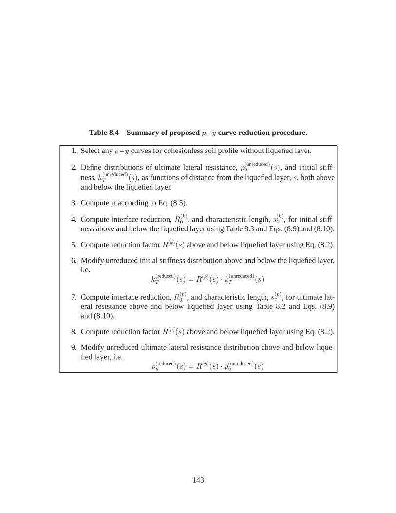
Table 8.4 Summary of proposedp –y curve reduction procedure.

1. Select anyp –y curves for cohesionless soil profile without liquefied layer.

2. Define distributions of ultimate lateral resistance,p(unreduced)u (s), and initial stiff-

ness,k(unreduced)T (s), as functions of distance from the liquefied layer,s, both above

and below the liquefied layer.

3. Computeβ according to Eq. (8.5).

4. Compute interface reduction,R(k)0 , and characteristic length,s(k)c , for initial stiff-

ness above and below the liquefied layer using Table 8.3 and Eqs. (8.9) and (8.10).

5. Compute reduction factorR(k)(s) above and below liquefied layer using Eq. (8.2).

6. Modify unreduced initial stiffness distribution above and below the liquefied layer,i.e.

k(reduced)T (s) = R(k)(s) · k(unreduced)

T (s)

7. Compute interface reduction,R(p)0 , and characteristic length,s(p)c , for ultimate lat-

eral resistance above and below liquefied layer using Table 8.2 and Eqs. (8.9)and (8.10).

8. Compute reduction factorR(p)(s) above and below liquefied layer using Eq. (8.2).

9. Modify unreduced ultimate lateral resistance distribution above and below lique-fied layer, i.e.

p(reduced)u (s) = R(p)(s) · p(unreduced)

u (s)

143

9 Beam on Nonlinear Winkler FoundationAnalysis

9.1 INTRODUCTION

Beam on nonlinear Winkler foundation models are used to determine a suitable approach to asimplified analysis of a pile subject to a lateral spreading event. It has been shown that commonmethods used to definep –y curves for cohesionless soils estimatep –y curves with distributionsof ultimate lateral resistance,pu, and initial stiffness,kT , which are generally larger than corre-sponding distributions computed using 3D FE analysis. To assess how these increased parameterdistributions affect the simulated pile response, thep –y curves are used in lateral spreading anal-yses using a BNWF approach.

The BNWF model allows for direct comparison of the effects ofusing particular sets ofp –y curvesin a lateral spreading analysis. There are several purposesfor the BNWF analyses in this research:

1. Verification that thep –y curves obtained from 3D FE analysis are representative of the 3Dsoil response and are applicable to alternative pile deformation patterns. The pile bendingresponse obtained from BNWF analyses of lateral spreading using the computedp –y curvesare compared to corresponding results from 3D lateral spreading analysis.

2. Evaluation of the applicability ofp –y curves defined using predicted distributions ofpu andkT to lateral spreading simulation using a BNWF approach. The simulated pile responseobtained from BNWF analyses using these curves are comparedto 3D FE analysis and theBNWF analyses using computedp –y curves.

3. Verification of the effectiveness of the proposed reduction procedure to properly modifyp –y curves to account for the presence of a liquefied layer in a general soil profile. Thereduction procedure is applied top –y curves computed from 3D models with homogenoussoil profiles. The pile response obtained from a BNWF lateralspreading analysis using thesereducedp –y curves is compared to 3D results for a corresponding soil profile.

4. Identification of a simplified analysis procedure appropriate for the analysis of liquefaction-induced lateral spreading. Recommendations for the selection of predictedpu andkT dis-tributions are made via comparison of the simulated pile bending response obtained usingBNWF analysis withp –y curves defined using various approaches to the 3D FE analysisresults.

145

Each of these items are addressed via simulation of lateral spreading using a BNWF approach. Tothis purpose, a general BNWF model is developed in OpenSees.The results of these simulationsare used to make recommendations for the simplified analysisof lateral spreading using a BNWFmodel.

9.2 EVALUATION OF COMPUTED AND PREDICTED p –y CURVES

Evaluation of the computed and conventionalp –y curves in the context of the lateral spreadingproblem is conducted using a series of BNWF models. These models replace the soil continuumsurrounding the pile with a series of nonlinear springs withbehavior defined byp –y curves. Theresults of the BNWF analyses are compared to each other and tothe benchmark 3D results dis-cussed in Chapter 5 with respect to the bending response of the pile.

9.2.1 Beam on Nonlinear Winkler Foundation Model

In the BNWF model, three sets of nodes exist in the same set of locations. There are the pilenodes, which are connected to each other via beam elements, and two sets of spring nodes. Thenodes on the pile side of the springs are slave nodes to the pile nodes, sharing equal displacement(no rotation) with those nodes. The nodes on the soil side of the springs are held initially fixed.To simulate a lateral spreading event, an imposed displacement profile matching that used in the3D lateral spreading models, is applied to the soil end of thenonlinear springs. This approachis similar to that used by Brandenberg et al. (2007). A schematic illustrating the BNWF model isprovided in Figure 9.1. For the evaluation simulations, thesoil stiffness is assumed to be negligiblein the liquefied layer and thus is set to zero. The BNWF model utilizes the same beam elements asthe 3D models, with both linear elastic and elastoplastic constitutive formulations.

Pile node

Equal DOF Imposed displacementprofile

No springs inliquefied layer

Fixed

∆

Figure 9.1 Schematic representation of the BNWF model.

146

9.2.2 Modeling thep –y Curves

Thep –y curves are defined in OpenSees using zero-length elements and the providedPySimple1constitutive model, which allows for the definition ofp –y curves for both cohesive and cohesion-less soils. ThePySimple1constitutive model is based upon the work of Boulanger et al.(1999)in modeling seismic soil-pile-structure interaction. This constitutive model has an initially linearforce density-displacement relationship and plastic force density-displacement behavior describedby

p(yp) = pu − (pu − p0)

[

cy50cy50 + | yp − yp0|

]n

(9.1)

in which pu is the ultimate lateral resistance,y50 is the the lateral displacement at which one-halfof pu has been mobilized during monotonic loading, andp0 and yp0 are the values ofp andyp

at the beginning of the current plastic loading cycle, respectively. The constant,c, controls thetangent modulus at the onset of plastic yielding and the constant,n, controls the sharpness of thep –y curve. In order to closely approximate the shape of the API (1987) recommended curves fordrained sand, Boulanger et al. recommend settingc = 0.5 andn = 2.

Appropriate values ofpu andy50 must be defined as input values at each pile node. The establishedpu values can be used directly in OpenSees, however, the necessary values ofy50 are not inherentlydefined. Sensible values of this parameter are determined from Equation (6.1) by solving for thedisplacement at which the force is equal to one-half ofpu, resulting in

y50 =pukT

tanh−1(0.5) (9.2)

which definesy50 in terms of the known values ofkT andpu at each depth. A similar procedure isutilized to obtain suitable values of the parametery50 for the computedp –y curves. It is importantto note that in thePySimple1model, the input values ofpu must be in units of force instead of thecommonly-used units of force/length. Appropriate values are obtained through multiplication withthe tributary lengths discussed in Section 6.2.

9.2.3 Consideredp –y Curves

There are two series of BNWF models used to evaluate thep –y curves. In the first, the springshave behavior defined using thep –y curves computed from the 3D simulations. In the second,the springs are defined byp –y curves established using the API (1987) recommendations. Threepile diameters are considered (0.61 m, 1.37 m, 2.5 m), and theanalyses are split into two separatecases:

1. Homogenous Case: The p –y curves are not reduced to account for the presence of theliquefied layer. Computedp –y curves are obtained from homogenous soil profiles and theAPI curves are left unmodified.

2. Reduced Case: Thep –y curves reflect the influence of the liquefied layer. Computedp –ycurves are obtained from layered soil profiles with a liquefied middle layer. Thepu dis-tributions of the API curves are reduced through multiplication with thepu ratios obtained

147

Table 9.1 Overview of the considered BNWF analysis cases foreach pile.

FE analysis Curves API CurvesReduced Homogenous Reduced Homogenous

Elastic Pile X X X XElastoplastic Pile X X X X

through comparison of thep –y curves computed from homogenous and liquefied soil pro-files (see Figure 8.2).

Because the API curves have been shown to be too stiff with depth, the lowest recommendedsubgrade reaction coefficient,k = 5000 kN/m3, is used to define the initial stiffness of the APIcurves. This value does not correspond to the internal friction angle used in the soil constitutivemodel, however, it increases the applicability of the API curves to the lateral spreading case. Thepu distributions used for these curves are computed using soilproperties matching those used asinput values in the 3D model. The reductions made to these curves in the reduced analysis case,while not included in the API recommendations, creates a more realistic distribution ofp –y withdepth and enhances the applicability of the API curves to thelateral spreading case.

All of these cases are analyzed two times, once with elastic beam elements and once with elasto-plastic beam elements, creating a total of 24 distinct cases. A brief overview of the consideredcases is presented in Table 9.1.

9.2.4 Results

The results of the BNWF analyses are evaluated with respect to the maximum shear force,max V ,maximum bending moment,maxM , and the maximum curvature,maxφ, in the pile. The max-imum pile deflection,maxU , and the effective length,Leff , which is the distance between theextreme moment demands in the pile, are also considered. Tables 9.2, 9.3, and 9.4 summarize theresults of the BNWF analyses for a 2.5-m, a 1.37-m, and a 0.61-m-diameter pile, respectively.

148

Table 9.2 Pile bending response summary for BNWF analysis with a 2.5-m-diameter pile.

Elastic Pile Cases

Curve Type maxV (kN) maxM (kNm) maxφ (m−1) maxU (m) Leff (m)

FE analysis, homogenous 50900 285100 0.0015 1.65 16.30FE analysis, reduced 46700 278900 0.0014 1.64 16.40API, homogenous 175000 950100 0.0048 1.96 13.10API, reduced 150000 920600 0.0047 1.94 13.20

Elastoplastic Pile Cases




Elastic Pile Cases






149


Elastic Pile Cases






The maximum shear force, bending moment, and curvature demands returned using the API curvestend to be significantly larger than those returned by the FE analysis. As the pile diameter de-creases, the results become more similar, however, the API curves still predict larger demands forthe smallest pile. The effective lengths obtained using theAPI p –y curves tend to be smaller thanthose returned by the extracted curves, indicative of larger extreme bending demands on the piles.

In the elastoplastic pile cases, the maximum bending moments returned using the two sets ofp –y curves are similar due to the fact that the piles are reachingtheir moment capacity, however,the curvature demands placed upon the piles using the API curves are significantly larger and theeffective lengths tend to be shorter. Both of these results indicate that the bending demands on thepiles using the API curves are much more severe than those obtained using the FE analysis curves.

The BNWF results are compared to corresponding results obtained from the 3D modeling effort(see Chapter 5) in Tables 9.5, 9.6, and 9.7, which show the relative error between the BNWFand 3D pile bending demands. The elastic pile BNWF cases are compared to the results of thefree-head 3D Series3 cases, which consider elastic piles in elastoplastic soil.The elastoplasticBNWF cases are compared to the free-head 3D Series4 cases, which model elastoplastic piles inelastoplastic soil. As a reference, the 3D results for both the Series3 and4 cases are summarizedin Tables 5.2-5.4 (pages 69-69).

When applied to BNWF models, thep –y curves computed from the 3D FE analysis return piledemands that are reasonably similar to 3D lateral spreadingsimulations. There is a relatively smallamount of error which can be attributed to inaccuracies in the curve extraction procedure, the trans-fer of these extracted curves into the nonlinear spring models, and the inherent error in representinga 3D soil continuum with a series of discrete springs. This similarity in the results validates that thep –y curves computed using the rigid pile kinematic case in 3D, which are free from the influenceof pile kinematics, can be used successfully in a simplified BNWF lateral spreading analysis.

150

Table 9.5 Relative error between BNWF and 3D FE results for 2.5-m-diameter pile.

Elastic Pile Cases Relative ErrorCurve Type max V (%) maxM (%) maxφ (%) Leff (%)FE analysis, homogenous 5.80 5.10 3.20 1.20FE analysis, reduced 13.7 7.20 5.30 1.50API, homogenous 223 216 222 18.7API, reduced 177 206 212 18.1

Elastoplastic Pile Cases Relative ErrorCurve Type max V (%) maxM (%) maxφ (%) Leff (%)FE analysis, homogenous 5.30 3.30 14.0 3.75FE analysis, reduced 13.2 4.40 17.9 4.40API, homogenous 90.2 5.60 2350 40.0API, reduced 61.7 5.70 1750 33.4


Elastic Pile Cases Relative ErrorCurve Type max V (%) maxM (%) maxφ (%) Leff (%)FE analysis, homogenous 1.00 3.86 3.18 9.20FE analysis, reduced 11.1 5.97 5.30 10.3API, homogenous 111 95.9 97.3 14.4API, reduced 73.3 85.1 86.4 12.8

Elastoplastic Pile Cases Relative ErrorCurve Type max V (%) maxM (%) maxφ (%) Leff (%)FE analysis, homogenous 15.7 6.20 63.8 13.3FE analysis, reduced 19.9 5.55 8.71 6.78API, homogenous 18.1 5.17 46.5 31.7API, reduced 8.87 6.02 182 30.4


Elastic Pile Cases Relative ErrorCurve Type max V (%) maxM (%) maxφ (%) Leff (%)FE analysis, homogenous 7.25 0.83 0.94 2.41FE analysis, reduced 7.45 4.59 4.70 5.02API, homogenous 33.3 57.3 57.2 6.82API, reduced 6.07 47.6 47.4 4.03

Elastoplastic Pile Cases Relative ErrorCurve Type max V (%) maxM (%) maxφ (%) Leff (%)FE analysis, homogenous 2.92 0.59 14.7 2.08FE analysis, reduced 11.0 2.90 4.36 5.65API, homogenous 13.0 0.42 496 20.6API, reduced 4.43 1.96 253 7.34

151

Moment M (kN)

Hei

ght a

bove

bas

e (m

)

−4 −2 0 2x 10

4

0

5

10

15

20

25ComputedAPI3D FEA

Shear force V (kN)

Hei

ght a

bove

bas

e (m

)

−20000 −10000 00

5

10

15

20

25

ComputedAPI3D FEA

pile deflection (m)

Hei

ght a

bove

bas

e (m

)

0 0.5 10

5

10

15

20

25

ComputedAPI3D FEA

(a) (b) (c)

Figure 9.2 Deflected shape, shear force, and moment diagramsfor BNWF and 3D FE anal-yses of lateral spreading for a 1.37-m-diameter pile with linear elastic behavior.

The API p –y curves, which are inherently tied to a top pushover type of pile deformation, tendto be significantly larger than the 3D FE analysis results, even with the modifications made toenhance the applicability of these curves. The deflected pile shapes shown in Figure 9.2 emphasizethe effects of the overestimated stiffness in the API curves. As shown, when the computed curvesare used, the base of the pile is able to cut backwards into thesoil, just as is observed in the 3Dmodel. When this occurs, the pile has a degree of rigid body rotation in its deformation profile,lessening the curvature demands incurred during the lateral spreading event. Using the API curvesleads to a condition in which the base of the pile is held firmlyin place during the lateral spreadingevent, increasing the curvature demands on the pile, especially in the lower solid layer.

The shear and moment diagrams of Figure 9.2 further demonstrate the differences in pile responsefor the two sets ofp –y curves. The diagrams corresponding to the computedp –y curves aresimilar to those corresponding to the 3D FE analysis, while the API curves predict significantlylarger shear and moment demands over the full length of the pile.

The results of the elastoplastic pile analyses demonstrateanother relative difference between theanalysis approaches. As shown in Figure 9.2, there are two extreme moment demands, one ineach unliquefied soil layer. Figure 9.3 shows the evolution of these extreme pile moments obtainedfrom the 3D FE analysis and BNWF models with computed and APIp –y curves. As a result ofthe response overpredictions inherent to the API curves, significantly larger curvature demands areplaced on the pile and large curvatures develop much earlierin the lateral spreading deformation.The API-based analysis indicates that the pile has reached its moment capacity when the upperlayer has displaced approximately 0.24 m (≈ 0.18 diameters) relative to the lower layer. In thecomputedp –y curve and 3D analyses, the pile moment capacity is reached atabout 0.48 m (≈0.35 diameters) of upper soil layer displacement. This is a significant difference in perceived pilebending demand between the cases, even with the assumed lateral resistance reductions in the APIcurves near the liquefied layer.

It is recommended thatp –y curves defined using the API (1987) recommendations not be used ina simplified analysis of piles for lateral spreading. The BNWF analyses have shown that the com-putedp –y curves produce similar results to the 3D model and that thereare significant differencesbetween the results obtained using the computed and APIp –y curves, even with modificationsto the API curves, which serve to increase their applicability to the lateral spreading case. The

152

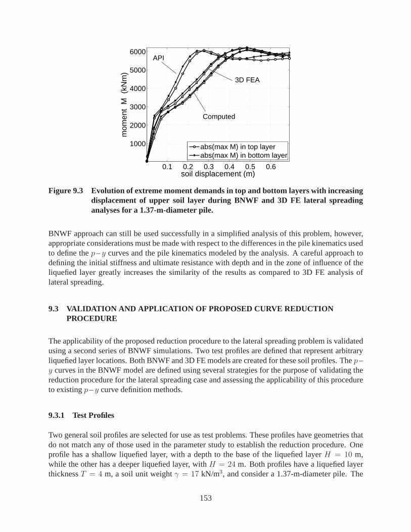
0.1 0.2 0.3 0.4 0.5 0.6

1000

2000

3000

4000

5000

6000

soil displacement (m)

mom

ent

M (

kNm

)


API

Computed

3D FEA

Figure 9.3 Evolution of extreme moment demands in top and bottom layers with increasingdisplacement of upper soil layer during BNWF and 3D FE lateral spreadinganalyses for a 1.37-m-diameter pile.

BNWF approach can still be used successfully in a simplified analysis of this problem, however,appropriate considerations must be made with respect to thedifferences in the pile kinematics usedto define thep –y curves and the pile kinematics modeled by the analysis. A careful approach todefining the initial stiffness and ultimate resistance withdepth and in the zone of influence of theliquefied layer greatly increases the similarity of the results as compared to 3D FE analysis oflateral spreading.

9.3 VALIDATION AND APPLICATION OF PROPOSED CURVE REDUCTIONPROCEDURE

The applicability of the proposed reduction procedure to the lateral spreading problem is validatedusing a second series of BNWF simulations. Two test profiles are defined that represent arbitraryliquefied layer locations. Both BNWF and 3D FE models are created for these soil profiles. Thep –y curves in the BNWF model are defined using several strategiesfor the purpose of validating thereduction procedure for the lateral spreading case and assessing the applicability of this procedureto existingp –y curve definition methods.

9.3.1 Test Profiles

Two general soil profiles are selected for use as test problems. These profiles have geometries thatdo not match any of those used in the parameter study to establish the reduction procedure. Oneprofile has a shallow liquefied layer, with a depth to the base of the liquefied layerH = 10 m,while the other has a deeper liquefied layer, withH = 24 m. Both profiles have a liquefied layerthicknessT = 4 m, a soil unit weightγ = 17 kN/m3, and consider a 1.37-m-diameter pile. The

153

unliquefied soil layers have an internal friction angleφ = 38◦. The remaining soil propertiesare as listed in Table 4.2. 3D models are created for each testprofile. These models are usedto computep –y curves using the rigid pile kinematic as well as to simulate lateral spreading inseparate analyses.

Separate BNWF models are created for each of the test profiles. These models are similar to thatdepicted in Figure 9.1, however, in the BNWF analyses used toassess the proposed reductionprocedure both the ultimate resistance and initial stiffness of thep –y curves in the liquefied layerare taken to be 10% of their unreduced magnitudes.

9.3.2 Investigated Test Cases

Thep –y curves used to describe the soil-pile interaction in the BNWF models are defined usingfive distinct combinations ofpu andkT distributions. The five resulting test cases include twovalidation cases (VC1andVC2), modeled using parameters directly obtained from the 3D rigid pilesimulations, and three practical cases (PC1, PC2, andPC3), modeled usingpu andkT distributionsestimated using methods readily available to practitioners. The investigated cases are summarizedbelow. Figures 9.4 and 9.5 show the distributions ofpu andkT , respectively, used for each testcase.

• Validation cases

– VC1: Thep –y curves in this case are defined using distributions ofpu andkT computeddirectly from the 3D model, resulting inp –y curves which are reduced for the presenceof the liquefied layer specifically for each respective soil profile.

– VC2: This case usesp –y curves withpu andkT distributions computed from a ho-mogenous soil 3D model in which the soil has the properties ofthe unliquefied layersin the test profiles. These curves are reduced for the presence of the liquefied layerusing the proposed reduction procedure.

• Practical cases

– PC1: Thep –y curves for this case are determined using the API recommendations (1987).The curves representing the unliquefied sand are not reducedfor the presence of the liq-uefied layer.

– PC2: This case uses a distribution ofpu defined using the method of Brinch Hansen(1961) and akT distribution defined by correcting the API distribution foroverburdenpressure after Boulanger et al. (2003). No reduction is madeto account for the presenceof the liquefied layer.

– PC3: This case uses thepu andkT distributions of casePC2with the proposed reduc-tion procedure applied to account for the presence of the liquefied layer.

The validation cases are intended to test the applicabilityof the BNWF model and the proposedreduction procedure to the lateral spreading load case. Thep –y curves forVC1 are obtained

154

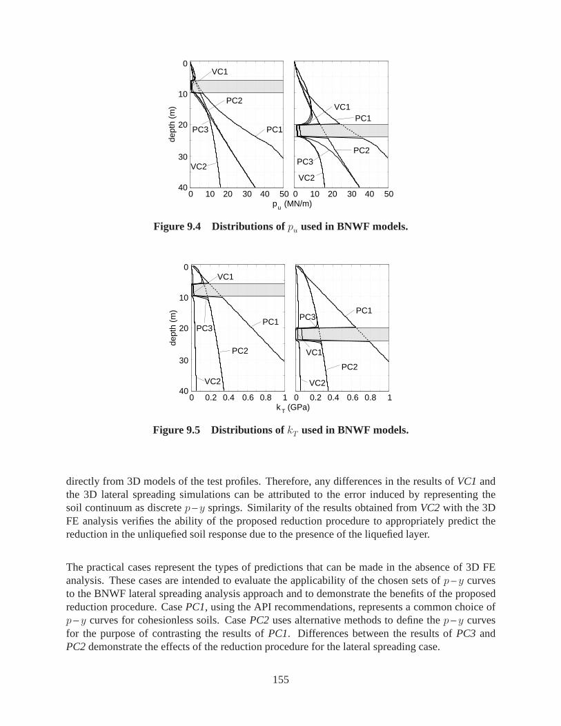
0 10 20 30 40 50

10

30

40

dept

h (m

)

VC1

PC1

VC2

PC2

20

VC2

PC2PC3

PC1VC1

0

0 10 20 30 40 50p (MN/m)u

PC3

Figure 9.4 Distributions of pu used in BNWF models.

10

30

40

dept

h (m

)

20

VC1

VC2

PC2

PC1PC3

VC2

PC3

VC1

PC2

PC1

0

0 0.2 0.4 0.6 0.8 1 0 0.2 0.4 0.6 0.8 1k (GPa)T

Figure 9.5 Distributions of kT used in BNWF models.

directly from 3D models of the test profiles. Therefore, any differences in the results ofVC1andthe 3D lateral spreading simulations can be attributed to the error induced by representing thesoil continuum as discretep –y springs. Similarity of the results obtained fromVC2with the 3DFE analysis verifies the ability of the proposed reduction procedure to appropriately predict thereduction in the unliquefied soil response due to the presence of the liquefied layer.

The practical cases represent the types of predictions thatcan be made in the absence of 3D FEanalysis. These cases are intended to evaluate the applicability of the chosen sets ofp –y curvesto the BNWF lateral spreading analysis approach and to demonstrate the benefits of the proposedreduction procedure. CasePC1, using the API recommendations, represents a common choiceofp –y curves for cohesionless soils. CasePC2 uses alternative methods to define thep –y curvesfor the purpose of contrasting the results ofPC1. Differences between the results ofPC3 andPC2demonstrate the effects of the reduction procedure for the lateral spreading case.

155

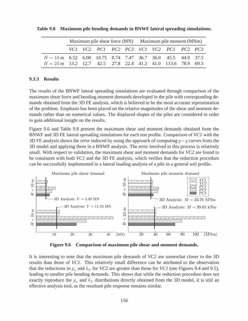
Table 9.8 Maximum pile bending demands in BNWF lateral spreading simulations.

Maximum pile shear force (MN) Maximum pile moment (MNm)

VC1 VC2 PC1 PC2 PC3 VC1 VC2 PC1 PC2 PC3

H = 10 m 6.52 6.00 10.75 8.74 7.47 36.7 36.0 45.5 44.0 37.5H = 24 m 13.2 12.7 42.5 27.8 22.4 41.2 41.0 113.6 78.9 69.3

9.3.3 Results

The results of the BNWF lateral spreading simulations are evaluated through comparison of themaximum shear force and bending moment demands developed inthe pile with corresponding de-mands obtained from the 3D FE analysis, which is believed to be the most accurate representationof the problem. Emphasis has been placed on the relative magnitudes of the shear and moment de-mands rather than on numerical values. The displaced shapesof the piles are considered in orderto gain additional insight on the results.

Figure 9.6 and Table 9.8 present the maximum shear and momentdemands obtained from theBNWF and 3D FE lateral spreading simulations for each test profile. Comparison ofVC1with the3D FE analysis shows the error induced by using the approach of computingp –y curves from the3D model and applying them in a BNWF analysis. The error involved in this process is relativelysmall. With respect to validation, the maximum shear and moment demands forVC2are found tobe consistent with bothVC1and the 3D FE analysis, which verifies that the reduction procedurecan be successfully implemented in a lateral loading analysis of a pile in a general soil profile.

��

��

��

��

��

��

��

��

��

��

VC1VC2PC1PC2PC3

(MN)40302010

H=

24

mH

=10

m

3D Analysis: V = 5.49 MN

3D Analysis: V = 11.53 MN

H=

24m

H=

10m

20 40 60 80 100 (MNm)

3D Analysis: M = 33.76 MNm

3D Analysis: M = 39.05 kNm

Maximum pile moment demandMaximum pile shear demand

Figure 9.6 Comparison of maximum pile shear and moment demands.

It is interesting to note that the maximum pile demands ofVC2 are somewhat closer to the 3Dresults than those ofVC1. This relatively small difference can be attributed to the observationthat the reductions inpu andkT for VC2are greater than those forVC1 (see Figures 9.4 and 9.5),leading to smaller pile bending demands. This shows that while the reduction procedure does notexactly reproduce thepu andkT distributions directly obtained from the 3D model, it is still aneffective analysis tool, as the resultant pile response remains similar.

156

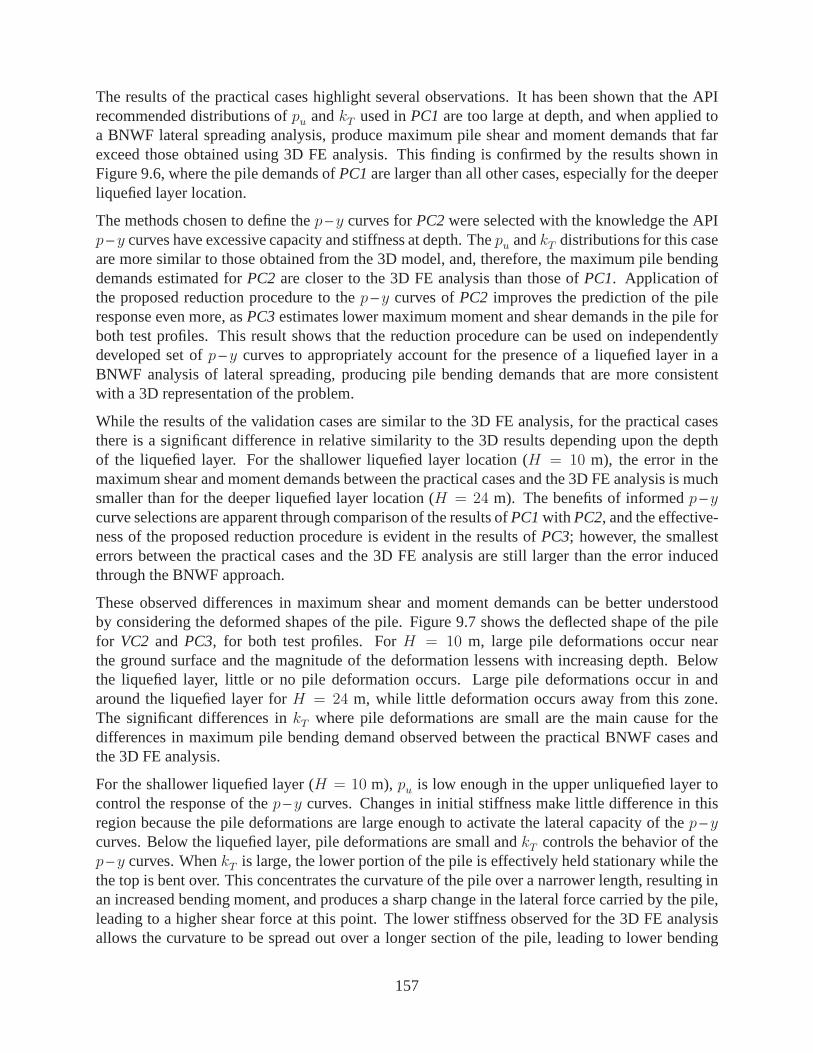
The results of the practical cases highlight several observations. It has been shown that the APIrecommended distributions ofpu andkT used inPC1are too large at depth, and when applied toa BNWF lateral spreading analysis, produce maximum pile shear and moment demands that farexceed those obtained using 3D FE analysis. This finding is confirmed by the results shown inFigure 9.6, where the pile demands ofPC1are larger than all other cases, especially for the deeperliquefied layer location.

The methods chosen to define thep –y curves forPC2were selected with the knowledge the APIp –y curves have excessive capacity and stiffness at depth. Thepu andkT distributions for this caseare more similar to those obtained from the 3D model, and, therefore, the maximum pile bendingdemands estimated forPC2 are closer to the 3D FE analysis than those ofPC1. Application ofthe proposed reduction procedure to thep –y curves ofPC2 improves the prediction of the pileresponse even more, asPC3estimates lower maximum moment and shear demands in the pileforboth test profiles. This result shows that the reduction procedure can be used on independentlydeveloped set ofp –y curves to appropriately account for the presence of a liquefied layer in aBNWF analysis of lateral spreading, producing pile bendingdemands that are more consistentwith a 3D representation of the problem.

While the results of the validation cases are similar to the 3D FE analysis, for the practical casesthere is a significant difference in relative similarity to the 3D results depending upon the depthof the liquefied layer. For the shallower liquefied layer location (H = 10 m), the error in themaximum shear and moment demands between the practical cases and the 3D FE analysis is muchsmaller than for the deeper liquefied layer location (H = 24 m). The benefits of informedp –ycurve selections are apparent through comparison of the results ofPC1with PC2, and the effective-ness of the proposed reduction procedure is evident in the results ofPC3; however, the smallesterrors between the practical cases and the 3D FE analysis arestill larger than the error inducedthrough the BNWF approach.

These observed differences in maximum shear and moment demands can be better understoodby considering the deformed shapes of the pile. Figure 9.7 shows the deflected shape of the pilefor VC2 and PC3, for both test profiles. ForH = 10 m, large pile deformations occur nearthe ground surface and the magnitude of the deformation lessens with increasing depth. Belowthe liquefied layer, little or no pile deformation occurs. Large pile deformations occur in andaround the liquefied layer forH = 24 m, while little deformation occurs away from this zone.The significant differences inkT where pile deformations are small are the main cause for thedifferences in maximum pile bending demand observed between the practical BNWF cases andthe 3D FE analysis.

For the shallower liquefied layer (H = 10 m), pu is low enough in the upper unliquefied layer tocontrol the response of thep –y curves. Changes in initial stiffness make little difference in thisregion because the pile deformations are large enough to activate the lateral capacity of thep –ycurves. Below the liquefied layer, pile deformations are small andkT controls the behavior of thep –y curves. WhenkT is large, the lower portion of the pile is effectively held stationary while thethe top is bent over. This concentrates the curvature of the pile over a narrower length, resulting inan increased bending moment, and produces a sharp change in the lateral force carried by the pile,leading to a higher shear force at this point. The lower stiffness observed for the 3D FE analysisallows the curvature to be spread out over a longer section ofthe pile, leading to lower bending

157

VC2PC3

1.5pile displacement (m)

1.00.50−0.5 1.5 −0.5 0 0.5 1.0

H = 24 mH = 10 m

10

0

20

30

dept

h (m

)

Figure 9.7 Deformed shapes of pile in theVC2 and PC3BNWF analyses.

demands. These differences in the displaced shape of the pile are highlighted in Figure 9.7 for twoanalysis cases.

Similar behavior leads to the large bending demands observed with a deeper liquefied layer (H =24 m), however, the depth of the liquefied layer alters the displacement profile of the pile suchthat two hinges form, whereas only a single hinge developed for the shallow liquefied layer. Thecombined effect of two hinges and higher values ofpu andkT at depth for the practical cases leadsto the large discrepancies compared to the 3D FE analysis. Asshown in Figure 9.7, compared toVC2, the hinge points forPC3 are closer to the liquefied layer and the curvature is concentratedover shorter lengths, both of which are due to the larger values ofpu andkT for this case. For adeeper liquefied layer location, the selection ofp –y curves used in the BNWF analysis signifi-cantly affects the simulated pile response. Careful selection of p –y curves is critical to obtainingan accurate estimate of the maximum pile bending demands.

9.4 EFFECTS OF SOIL SHEAR MODULUS ON INITIAL STIFFNESS OF p –yCURVES

The results of the BNWF analyses have shown that the maximum bending demands placed on apile during a lateral spreading event have a strong dependence on the initial stiffness of the soilresponse. As shown in Figure 9.5, thekT distribution computed from the 3D model is significantlylower than either of the estimated distributions. The difference is due to how these distributionsare determined. The API initial stiffness distribution is defined as a function of the friction angle,φ, of the soil, whereas in the 3D model, the initial stiffness is a function of the shear modulus,G,of the soil constitutive model.

Friction angle is a failure parameter related more topu , while kT is related more fundamentally toG; however, the friction angle and small strain shear modulusof an actual sand are both directlyrelated to the relative density, and therefore to each other, so defining the initial stiffness of thep –y curves based onφ is reasonable. No such intrinsic relation betweenφ andG exists in theDrucker-Prager constitutive model. In an actual sand, the shear modulus decreases with increasingshear strain. Because the constitutive model used in the simulations does not directly considermodulus reduction, the shear modulus of the unliquefied layers must be taken to represent a largestrain value. This indicates that comparisons made betweenvalues ofkT computed based on a

158

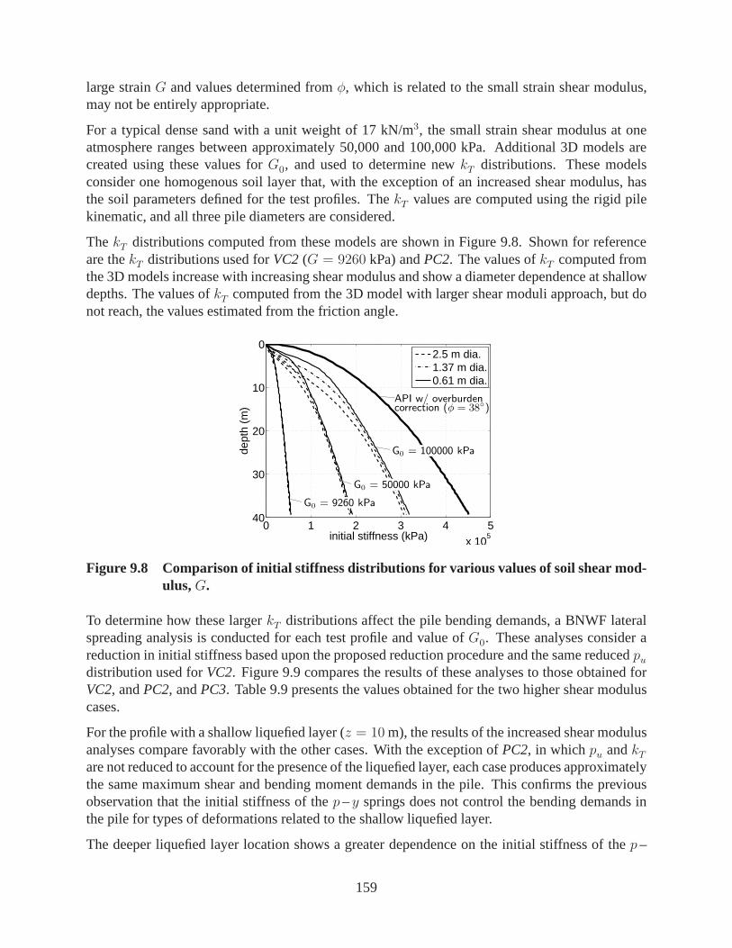
large strainG and values determined fromφ, which is related to the small strain shear modulus,may not be entirely appropriate.

For a typical dense sand with a unit weight of 17 kN/m3, the small strain shear modulus at oneatmosphere ranges between approximately 50,000 and 100,000 kPa. Additional 3D models arecreated using these values forG0, and used to determine newkT distributions. These modelsconsider one homogenous soil layer that, with the exceptionof an increased shear modulus, hasthe soil parameters defined for the test profiles. ThekT values are computed using the rigid pilekinematic, and all three pile diameters are considered.

ThekT distributions computed from these models are shown in Figure 9.8. Shown for referenceare thekT distributions used forVC2 (G = 9260 kPa) andPC2. The values ofkT computed fromthe 3D models increase with increasing shear modulus and show a diameter dependence at shallowdepths. The values ofkT computed from the 3D model with larger shear moduli approach, but donot reach, the values estimated from the friction angle.

0 1 2 3 4 5x 10

5

0

10

20

30

40


dept

h (m

)

2.5 m dia.1.37 m dia.0.61 m dia.

API w/ overburdencorrection (φ = 38

◦)

G0 = 100000 kPa

G0 = 50000 kPa

G0 = 9260 kPa

Figure 9.8 Comparison of initial stiffness distributions for various values of soil shear mod-ulus,G.

To determine how these largerkT distributions affect the pile bending demands, a BNWF lateralspreading analysis is conducted for each test profile and value ofG0. These analyses consider areduction in initial stiffness based upon the proposed reduction procedure and the same reducedpudistribution used forVC2. Figure 9.9 compares the results of these analyses to those obtained forVC2, andPC2, andPC3. Table 9.9 presents the values obtained for the two higher shear moduluscases.

For the profile with a shallow liquefied layer (z = 10 m), the results of the increased shear modulusanalyses compare favorably with the other cases. With the exception ofPC2, in whichpu andkTare not reduced to account for the presence of the liquefied layer, each case produces approximatelythe same maximum shear and bending moment demands in the pile. This confirms the previousobservation that the initial stiffness of thep –y springs does not control the bending demands inthe pile for types of deformations related to the shallow liquefied layer.

The deeper liquefied layer location shows a greater dependence on the initial stiffness of thep –

159

��

��

��

��

��

��

��

��

��

��

5 10 15 20 25 30 10 20 30 40 50 60 70 80

H=

24m

H=

10m

H=

10m

H=

24m

Maximum pile shear demand Maximum pile moment demand

(MN)

VC2PC2PC3G0 = 50 MPaG0 = 100 MPa

(MNm)

Figure 9.9 Comparison of maximum pile shear and moment demands for higher shearmodulus cases.

Table 9.9 Maximum pile bending demands in BNWF lateral spreading simulations forhigher shear modulus cases.

Maximum pile shear force (MN) Maximum pile moment (MNm)

G0 = 50 MPa G0 = 100 MPa G0 = 50 MPa G0 = 100 MPa

H = 10 m 6.28 7.12 36.6 37.1H = 24 m 20.1 22.0 61.5 67.9

y springs. The maximum shear and moment demands in the pile increase with increasingG0,and the practical cases, which have even largerkT distributions, produce bending demands thatare greater still. For both of the considered soil profiles, the bending demands predicted usingG0 = 100, 000 kPa, agree well with those estimated inPC3. This suggests that when workingunder the assumption of a small strain shear modulus, the combination ofpu andkT distributionprediction methods used forPC3, when reduced for the presence of the liquefied layer using theproposed reduction procedure, can be used to predict reasonable maximum shear and momentdemands in a BNWF lateral spreading analysis.

9.5 SUMMARY

Analysis of pile foundations subject to liquefaction-induced lateral spreads is difficult due to thecomplexity of the problem. Simplified BNWF analyses usingp –y curves are a common designtool for this load case. Careful and informed selection of thep –y curves for a particular analysis,as defined by the characteristicp –y curve parameters of ultimate lateral resistance,pu, and initialstiffness,kT , are crucial for the effectiveness of the BNWF approach.

When applied to BNWF models, thep –y curves computed from 3D FE analysis return pile de-mands that are reasonably similar to 3D lateral spreading simulations, thus validating the approachof computingp –y curves using the rigid pile kinematic. Usingp –y curves established using theprocedure recommended by the API, the piles in the BNWF models are subject to significantly

160

larger curvature demands than those returned by the 3D modeling effort. These curves are derivedbased upon tests of piles loaded at or near the ground surfaceonly, and it has been shown thatp –y curves established in this manner are not applicable to the alternative kinematic of the lateralspreading case in which relatively large pile displacements occur with depth.

Lateral spreading analyses were conducted using BNWF and 3DFE approaches to verify anddemonstrate the effectiveness of the proposedp –y curve reduction procedure. It was shown that aBNWF analysis usingp –y curves obtained from a homogenous soil profile and then reduced usingthe proposed procedure estimates maximum pile shear and moment demands which compared wellwith 3D FE analysis. It was also shown that the proposed reduction procedure, when applied to aBNWF lateral spreading analysis in tandem with an informed selection ofp –y curves, producedmaximum pile bending demands that were more similar to the 3Dresults than identical unreducedp –y curves. The effect of the magnitude of the soil shear moduluson the initial stiffness of thep –y curves computed from 3D FE analysis is considered, and it is observed that use of a small strainshear modulus estimates pile bending demands which are moresimilar to the practical methods.

Based upon this work, it is recommended that a BNWF analysis of liquefaction-induced lateralspreading be conducted usingp –y curves defined by thepu distribution of Brinch Hansen (1961)and the API (1987) distribution ofkT , corrected for overburden pressure after Boulanger et al.(2003), in conjunction with the reduction procedure described in this paper. Use ofp –y curvesdefined in this manner seems to estimate maximum pile shear and moment demands that correlatewell with a 3D representation of the problem, and will allow asimple BNWF analysis to producemore efficient design solutions.

161

10 Summary, Conclusions, andRecommendations for Future Work

This report presents a kinematic analysis of a single pile embedded in a laterally spreading layeredsoil profile. An evaluation of the relevancy of conventionalanalysis models to this load case isconducted, and a simplified design procedure using a BNWF approach is proposed.

10.1 SUMMARY AND CONCLUSIONS

A summary of the work and associated conclusions of this research is presented in terms of thefollowing items: FE model development, 3D lateral spreading analysis, representativep –y curvecomputation, evaluation of conventional and computedp –y curves, influence of liquefied layer,and BNWF analysis.


Chapters 2, 3, and 4 presented the majority of the finite element model development necessaryto this research. Additional variations on the main template model that consider increased lateralextents, near-surface effects, a plane strain condition, and variable soil profiles were developedand discussed in Chapters 6, 7, and 8. Each individual component of the models was validated toensure that verifiably-correct behavior is observed when simple load cases are applied. The mainaspects of this work are summarized as follows.

• A 3D soil-pile interaction model was created for the case of asingle pile embedded in asoil continuum. This model employs beam-column elements tomodel the piles, solid brickelements for the soil, and beam-solid contact elements to define the soil-pile interaction.

• Fiber section models were created for three template reinforced concrete pile designs. Thesemodels define the constitutive behavior for the beam-columnelements used to model thepiles. The moment-curvature responses of the composite elastoplastic fiber section modelswere verified by several means.

163

• The Drucker-Prager constitutive model used to define the elastoplastic behavior for the co-hesionless soils in the lateral spreading model was verifiedthrough the applications of stresspaths that simulate commonly-used geotechnical tests. It was confirmed that the Drucker-Prager model is able to produce predictable responses to theapplication of these stress paths.

• Variations in the main soil-pile interaction model were made in order to analyze specificbehaviors in greater detail. Models with extended lateral extents were developed and usedto evaluate the effects of the fixed boundary in the standard model. Near-surface and planestrain models were developed and analyzed in order to validate observations made usingthe standard mesh. Models without fixed liquefied layer locations were used to evaluate theinfluence of the liquefied layer on the soil response.

3D Lateral Spreading Analysis

As discussed in Chapter 5, 24 distinct analysis cases were considered for the lateral spreadingkinematic. These cases were divided into four analysis Series depending upon the combination ofconstitutive models assigned for the pile and soil elements. These four Series were analyzed fortwo boundary conditions at the head of the pile, fixed and free, resulting in eight analysis cases foreach of the three pile designs. Several findings were made based upon this modeling effort.

• For a pile subjected to the kinematic demands of the lateral spreading case, the maximumshear force demand develops at the center of the liquefied layer and there are two extrememoment demands, one in each solid soil layer. The maximum moment demand exists in thelower layer for all but one of the 24 considered cases. The distance between the extrememoments defines the effective length factor for the pile,Leff , a parameter that provides anindication of the severity of the bending demand.

• The liquefied interface acts similarly to a free surface and the adjacent solid soil is able to bepushed into the weaker center layer during the application of lateral loads. This effectivelyreduces the strength of the solid soil in the regions adjacent to the liquefied layer.

• Plastic hinges form in the pile at the locations of extreme moment in each layer. The plasticdeformation/rotation in these locations becomes concentrated over an increasingly smallerlength of the pile as the pile-to-soil stiffness ratio decreases.

• The fixity of the pile head is an important consideration. Cases analyzed using a fixedboundary condition at the top of the pile return larger bending moment demands in the pilesthan corresponding cases analyzed with a free-head condition. Additionally, the maximummoment demand does not generally exist at the point of fixity,but rather, occurs further downin the soil profile. This location depends upon the thicknessof the top layer, soil stiffness,and the bending stiffness of the pile.

• The consideration of elastoplastic soil behavior leads to larger estimated maximum momentsin the pile than occur with linear elastic soil elements due to the failure of the soil. Thisobservation has been confirmed through the use of two simple beam models, which can be

164

solved by hand in a relatively simple manner. Elastoplasticsoil behavior must be consideredin order to obtain appropriate maximum moment and shear demands for piles.

Representativep –y Curve Computation

The soil response obtained from the soil-pile interaction models is evaluated through the com-putation of representative force density-displacement (p - y) curves at each pile node using theprocedure described in Chapter 6. Smooth curves are fit to therecorded data using a least squarefit. Two functional forms are used: one to establish the initial tangent of thep –y curves and theother to define the complete shape of the curves. In addition to the lateral spreading case, twoalternative pile kinematic cases are considered: a top-pushover case and a rigid pile case in whichthere is a uniform displacement profile with depth. The effects of model-specific phenomena onthe extracted results are explored through investigationsof variations in the meshing and fixedboundaries. Several conclusions may be drawn from this computational process.

• The force density-displacement (p –y ) data returned by the 3D models can be fit reasonablywell using a hyperbolic tangent function, though the use of this functional form tends tounderestimate the initial stiffness displayed by the FE data. Initial stiffness can be establishedusing a polynomial curve fit.

• The kinematics of the pile plays an essential role in definingthe obtained soil response andcan significantly affect the computedp –y curves. The top-pushover and lateral spreadingcases produce pile displacement profiles that vary in magnitude over the length of the piles.At nodes for which the pile displacement is small, not only isthe soil response insufficientlyactivated, the comparably larger displacements which occur at adjacent nodes influence thesoil response at these nodes, leading top –y curves that are not representative of the truesoil response. The rigid pile kinematic case must be utilized in order to obtain sensible localp –y curves over the length of the pile.

• Selective mesh refinement results in a condition where the stiffness of the soil continuumvaries over the length of the pile. This inconsistent stiffness manifests itself as fluctuationsin the recorded soil response. Models with uniformly-sizedmeshes are analyzed and theinconsistent results obtained from the selectively refinedmeshes can be smoothened throughmultiplication with a ratio obtained using the uniform meshresults.

• The fixed boundaries in the model can influence the soil response at large drift. This isconfirmed through the use of an additional model created withincreased lateral extents inthe direction of pile loading. In the default meshes, the proximity of the pile to the boundarycauses confining stresses to develop in the deeper portions of the soil that are too large.This effect can be partially alleviated through the use of non-associative plasticity in the soilconstitutive model.

165

Evaluation of Conventional and Computedp –y Curves

The representativep –y curves computed from the 3D FE model using the procedures describedin Chapter 6 were used to evaluate several conventional means for describing soil response andestablishingp –y curves. The evaluation of the computedp –y curve parameter distributions andcomparisons with the conventional methods were discussed in Chapter 7. The considered methodsencompass several commonly referenced methods for the definition of distributions of ultimateresistance and initial stiffness with depth. Several observations were made from these comparisonsand about the extracted parameter distributions and the following conclusions are drawn.

• Depth appropriate soil failure modes must be considered in the distributions of both the initialstiffness and ultimate lateral resistance of the soil. Nearthe surface, the lack of overburdenpressure leads to the early onset of yield while at depth, theincreased overburden pressureleads to the expansion of the elastic regime in the soil. Bothof these factors significantlyinfluence both the initial stiffness and ultimate resistance of the computedp –y curves.

• The magnitudes of the computed curves are similar to severalof the considered methods atdifferent depths, however, the general form of the results is not reflected in the predicted dis-tributions. It is noted that the current model is not capturing the true ultimate resistance of thesoil at depths beyond a few meters. The extracted values beyond this point are extrapolatedby the curve-fitting procedure.

• The linear initial stiffness distribution with depth commonly assumed appears to be basedupon an extrapolated elastoplastic state. The predicted stiffness at shallow depths correlatesfairly well with the 3D FE results, though there is a diameter-dependence that is missing. Atincreased depths, there is no clear correlation between thecomputed and estimated results.

• The method most commonly employed when establishingp –y curves for a particular cohe-sionless soil, that recommended by the API (1987), overestimates both the initial stiffnessand ultimate lateral resistance of the soil at depth. This method is based upon field tests inwhich loads are applied at or above the ground surface. It is likely that the kinematics ofthe pile in this case contribute to the unrealistically large values that are predicted by thismethodology.

Influence of Liquefied Layer

The effects of a liquefied layer on the lateral response of a soil system are evaluated in Chapter8. This is accomplished through the comparison ofp –y curves computed from homogenous soilprofiles with corresponding curves computed from layered soil profiles in which a liquefied layeris located between two unliquefied soil layers. Several observations are made and conclusions aredrawn.

• The presence of a liquefied layer in the soil profile reduces the initial stiffness and ultimatelateral resistance of the unliquefied soil layers in the areas adjacent to the weaker liquefiedmiddle layer.

166

• It is observed that the reduction is greatest at the layer interface and decays exponentiallywith increasing distance from the liquefied layer in both theupper and lower unliquefiedlayers. The magnitude of the reduction at a particular distance from the liquefied interfacedepends on the thickness of the liquefied layer, the diameterof the pile, and the verticaleffective stress.

• An exponential decay model is proposed to describe the observed parameter reductions.

• A parameter study using thep –y curves computed from 126 combinations of pile diame-ter, soil profile, and soil properties is used to develop a means to predict reductions for aparticular soil profile.

• A simplified procedure is proposed to estimate appropriate reductions in ultimate lateralresistance and initial stiffness for a given soil-pile system that includes a liquefied layer.

Beam on Nonlinear Winkler Foundation Analysis

Beam on nonlinear Winkler foundation analyses of lateral spreading are discussed in Chapter 9.These models are created in order to validate the computedp –y curves, to assess the applicabilityof conventionally-definedp –y curves to the lateral spreading case, and to validate/demonstratethe proposed procedure to reducep –y curves to account for the presence of a liquefied soil layer.Several observations and conclusions are made.

• Thep –y curves computed from 3D FE analysis produce simulated pile bending responses inBNWF analyses which compare well with corresponding results from 3D lateral spreadingsimulations. This validates thatp –y curves computed using the proposed rigid pile methodare representative of the soil response regardless of the analyzed pile kinematics.

• The overestimated values of ultimate lateral resistance and initial stiffness in the API (1987)recommendedp –y curves lead to very large pile bending demands that greatly exceed thoseobtained in 3D analysis. Use of these curves without modification for analysis of lateralspreading, or another load case with deep-seated soil-pileinteraction, is not recommended.

• The pile bending responses from BNWF analyses usingp –y curves computed from a ho-mogenous soil profile, then reduced using the proposed reduction procedure, compare favor-ably with corresponding 3D FE analyses that include a liquefied layer. This validates thatthe reduction procedure is able to estimate appropriate reductions for general combinationsof soil profile, soil properties, and pile diameter.

• Further BNWF simulation of lateral spreading identifies that among readily available meth-ods for defining distributions of ultimate lateral resistance and initial stiffness forp –ycurves, the method of Brinch Hansen (1961) and the modified API method proposed byBoulanger et al. (2003) seem to most accurately represent the soil response for the lateralspreading load case.

167

• Application of the proposed reduction process to the parameter distributions estimated bythese methods produces pile bending responses that more accurately represent corresponding3D FE results.

10.2 RECOMMENDATIONS FOR FUTURE WORK

There are several avenues for future work which are suggested by this research. Though manyfindings have been made, there are nearly as many unanswered questions. These recommendationsfor future work are subdivided into several categories for clarity.


• It may be advantageous to explore more combinations of soil and pile properties to furtherassess how these factors affect the simulations.

• The Drucker-Prager constitutive model used in the simulations is a relatively simple modelthat does not necessarily capture all aspects of the soil behavior. It may prove useful toexplore the findings of this research using a soil model that better captures the true soilbehavior.

• A large-deformation model may prove useful in fully capturing the ultimate soil behavior.

Experimental Need

• It may enhance the understanding of this problem to devise a way in which to perform aphysical lateral spreading test either at full, or nearly full, scale or at a reduced scale using ashaking table or a centrifuge. This would provide a second set of data with which to evaluatethe results of the numerical simulations.

• It has been observed that the soil response obtained from thenumerical simulations doesnot correlate with commonly used empirical methods for predicting this response, especiallyat depth. Perhaps physical tests, performed using a rigid pile kinematic, along with furthernumerical simulations can aid in the determination of suitable distributions of initial stiffnessand ultimate resistance over the length of the piles.

Soil Response Evaluation

• This research identified shortcomings of several conventional means for representing the lat-eral response of the soil with depth, however, this work is not conclusive enough to makefirm recommendations on revised distributions of ultimate lateral resistance and initial stiff-ness. Further numerical simulation, perhaps combined withexperimental study, would berequired for this purpose.

168

• This research focused on analyses conducted using a single pile embedded in a soil profilein which all surfaces are perpendicular to the pile and thereare only three layers. It wouldbe of interest to evaluate the applicability of these findings to any number of additional casessuch as pile groups, battered piles, sloping ground conditions, and increased number of soillayers. Any one of these investigations could prove to be a valuable contribution to thegeneral knowledge of laterally loaded piles.

169

REFERENCES

ACI Committee 318 (2005).Building Code Requirements for Structural Concrete (ACI 318–05)and Commentary (ACI 318R–05). American Concrete Institute, Farmington Hills, MI.

American Petroleum Institute (API) (1987).Recommended Practice for Planning, Designing andConstructing Fixed Offshore Platforms. API Recommended Practice 2A(RP–2A), Washington,D.C., 17th edition.

Bazant, Z. P. and Becq-Giraudon, E. (2002). “Statistical prediction of fracture parameters ofconcrete and implications for choice of testing standard.”Cement and Concrete Research, 32(4),529–556.

Boulanger, R. W., Curras, C. J., Kutter, B. L., Wilson, D. W.,and Abghari, A. (1999). “Seismicsoil–pile–structure interaction experiments and analyses.” Journal of Geotechnical and Geoen-vironmental Engineering, ASCE, 125(9), 750–759.

Boulanger, R. W., Kutter, B. L., Brandenberg, S. J., Singh, P., and Chang, D. (2003).Pile Foun-dations in liquefied and laterally spreading ground during earthquakes: Centrifuge experimentsand analyses. Center for Geotechnical Modeling, University of California at Davis, Davis, CA.Rep. UCD/CGM-03/01.

Brandenberg, S. J., Boulanger, R. W., Kutter, B. L., and Chang, D. (2007). “Static pushoveranalyses of pile groups in liquefied and laterally spreadingground in centrifuge tests.”Journalof Geotechnical and Geoenvironmental Engineering, ASCE, 133(9), 1055–1066.

Brinch Hansen, J. (1961). “The ultimate resistance of rigidpiles against transversal forces.”Bul-letin No. 12, Geoteknisk Institute, Copenhagen, 5–9.

Broms, B. B. (1964). “Lateral resistance of piles in cohesionless soils.”Journal of the Soil Me-chanics and Foundations Division, ASCE, 90(SM3), 123–156.

Brown, D. A. and Shie, C. F. (1990). “Three dimensional finiteelement model of laterally loadedpiles.” Computers and Geotechnics, 10(1), 59–79.

Chen, W. F. and Saleeb, A. F. (1994).Constitutive Equations for Engineering Materials Volume I:Elasticity and Modeling. Elsevier Science B.V., Amsterdam.

Drucker, D. C. and Prager, W. (1952). “Soil mechanics and plastic analysis or limit design.”Quarterly of Applied Mathematics, 10(2), 157–165.

Finn, W. D. L. and Fujita, N. (2002). “Piles in liquefiable soils: seismic analysis and design issues.”Soil Dynamics and Earthquake Engineering, 22(9-12), 731–742.

Fleming, W. G. K., Weltman, A. J., Randolph, M. F., and Elson,W. K. (1985).Piling Engineering.Surrey University Press, London.

171

Georgiadis, M. (1983). “Development ofp–y curves for layered soils.”Geotechnical Practice inOffshore Engineering, Reston, VA. ASCE, 536–545.

Helnwein, P. (2001). “Some remarks on the compressed matrixrepresentation of symmetricsecond-order and fourth-order tensors.”Computer Methods in Applied Mechanics and Engi-neering, 190(22-23), 2753 – 2770.

International Center for Numerical Methods in Engineering(CIMNE) (2008).GiD User Manual.http://gid.cimne.upc.es/.

Kaplan, M. F. (1961). “Crack propogation and the fracture ofconcrete.”Journal of the AmericanConcrete Institute, 58(5), 591–610.

Kent, D. C. and Park, R. (1971). “Flexural members with confined concrete.”Journal of theStructural Mechanics Division, ASCE, 97(ST7), 1969–1990.

Kulhawy, F. H. and Mayne, P. W. (1990).Manual on Estimating Soil Properties for FoundationDesign. Electrical Power Research Institute, EPRI EL–6800, Project 1493–6 Final Report.

Lam, I. P., Arduino, P., and Mackenzie-Helnwein, P. (2009).“Opensees soil–pile interaction studyunder lateral spread loading.”International Foundation Congress & Equipment Expo, Orlando,FL.

Matlock, H. and Reese, L. C. (1960). “Generalized solutionsfor laterally loaded piles.”Journal ofthe Soil Mechanics and Foundations Division, ASCE, 86(SM5), 63–91.

McClelland, B. and Focht, J. (1958). “Soil modulus for laterally loaded piles.”Transactions, ASCE,123, 1049–1086.

McGann, C. R., Arduino, P., and Mackenzie-Helnwein, P. (2010). “Lateral resistance reduction forstatic analysis of lateral spreading.”Joint Conference Proceedings, 7th International Conferenceon Urban Earthquake Engineering (7CUEE) & 5th International Conference on EarthquakeEngineering (5ICEE), Tokyo Institute of Technology, Tokyo, Japan.

Megson, T. H. G. (2005).Structural and Stress Analysis. Elsevier Butterworth Heinemann, Ams-terdam.

OpenSees. Open System for Earthquake Engineering Simulation. http://opensees.

berkeley.edu. Pacific Earthquake Engineering Research Center, University of California,Berkeley.

Park, R. and Paulay, T. (1975).Reinforced Concrete Structures. Wiley & Sons, New York.

Petek, K. A. (2006). “Development and application of mixed beam–solid models for analysis ofsoil–pile interaction problems,” Ph.d. thesis, University of Washington.

Reese, L. C., Cox, W. R., and Koop, F. D. (1974). “Analysis of laterally loaded piles in sand.”Proceedings of the 5th Offshore Technology Conference, Vol. 2, Houston. 473–483.

172

Reese, L. C. and Van Impe, W. F. (2001).Single Piles and Pile Groups Under Lateral Loading.A.A. Balkema, Rotterdam, Netherlands.

Scott, R. F. (1981).Foundation Analysis. Prentice–Hall, Englewood Cliffs, NJ.

Xu, S. and Zhang, X. (2008). “Determination of fracture parameters for crack propagation inconcrete using an energy approach.”Engineering Fracture Mechanics, 75(15), 4292–4308.

Yang, Z. and Jeremic, B. (2005). “Study of soil layering effects on lateral loading behavior ofpiles.” Journal of Geotechnical and Geoenvironmental Engineering, 131(6), 762–770.

173

PEER REPORTS

PEER reports are available individually or by yearly subscription. PEER reports can be ordered at http://peer.berkeley.edu/publications/peer_reports.html or by contacting the Pacific Earthquake Engineering Research Center, 325 Davis Hall mail code 1792, Berkeley, CA 94720. Tel.: (510) 642-3437; Fax: (510) 665-1655; Email: [email protected]

PEER 2012/05 Development of Simplified Analysis Procedure for Piles in Laterally Spreading Layered Soils. Christopher R. McGann, Pedro Arduino, and Peter Mackenzie–Helnwein. December 2012.

PEER 2012/04 Unbonded Pre-Tensioned Columns for Bridges in Seismic Regions. Phillip M. Davis, Todd M. Janes, Marc O. Eberhard, and John F. Stanton. December 2012.

PEER 2012/03 Experimental and Analytical Studies on Reinforced Concrete Buildings with Seismically Vulnerable Beam-Column Joints. Sangjoon Park and Khalid M. Mosalam. October 2012.

PEER 2012/02 Seismic Performance of Reinforced Concrete Bridges Allowed to Uplift during Multi-Directional Excitation. Andres Oscar Espinoza and Stephen A. Mahin. July 2012.

PEER 2012/01 Spectral Damping Scaling Factors for Shallow Crustal Earthquakes in Active Tectonic Regions. Sanaz Rezaeian, Yousef Bozorgnia, I. M. Idriss, Kenneth Campbell, Norman Abrahamson, and Walter Silva. July 2012.

PEER 2011/10 Earthquake Engineering for Resilient Communities: 2011 PEER Internship Program Research Report Collection. Eds. Heidi Faison and Stephen A. Mahin. December 2011.

PEER 2011/09 Calibration of Semi-Stochastic Procedure for Simulating High-Frequency Ground Motions. Jonathan P. Stewart, Emel Seyhan, and Robert W. Graves. December 2011.

PEER 2011/08 Water Supply in regard to Fire Following Earthquake. Charles Scawthorn. November 2011.

PEER 2011/07 Seismic Risk Management in Urban Areas. Proceedings of a U.S.-Iran-Turkey Seismic Workshop. September 2011.

PEER 2011/06 The Use of Base Isolation Systems to Achieve Complex Seismic Performance Objectives. Troy A. Morgan and Stephen A. Mahin. July 2011.

PEER 2011/05 Case Studies of the Seismic Performance of Tall Buildings Designed by Alternative Means. Task 12 Report for the Tall Buildings Initiative. Jack Moehle, Yousef Bozorgnia, Nirmal Jayaram, Pierson Jones, Mohsen Rahnama, Nilesh Shome, Zeynep Tuna, John Wallace, Tony Yang, and Farzin Zareian. July 2011.

PEER 2011/04 Recommended Design Practice for Pile Foundations in Laterally Spreading Ground. Scott A. Ashford, Ross W. Boulanger, and Scott J. Brandenberg. June 2011.

PEER 2011/03 New Ground Motion Selection Procedures and Selected Motions for the PEER Transportation Research Program. Jack W. Baker, Ting Lin, Shrey K. Shahi, and Nirmal Jayaram. March 2011.

PEER 2011/02 A Bayesian Network Methodology for Infrastructure Seismic Risk Assessment and Decision Support. Michelle T. Bensi, Armen Der Kiureghian, and Daniel Straub. March 2011.

PEER 2011/01 Demand Fragility Surfaces for Bridges in Liquefied and Laterally Spreading Ground. Scott J. Brandenberg, Jian Zhang, Pirooz Kashighandi, Yili Huo, and Minxing Zhao. March 2011.

PEER 2010/05 Guidelines for Performance-Based Seismic Design of Tall Buildings. Developed by the Tall Buildings Initiative. November 2010.

PEER 2010/04 Application Guide for the Design of Flexible and Rigid Bus Connections between Substation Equipment Subjected to Earthquakes. Jean-Bernard Dastous and Armen Der Kiureghian. September 2010.

PEER 2010/03 Shear Wave Velocity as a Statistical Function of Standard Penetration Test Resistance and Vertical Effective Stress at Caltrans Bridge Sites. Scott J. Brandenberg, Naresh Bellana, and Thomas Shantz. June 2010.

PEER 2010/02 Stochastic Modeling and Simulation of Ground Motions for Performance-Based Earthquake Engineering. Sanaz Rezaeian and Armen Der Kiureghian. June 2010.

PEER 2010/01 Structural Response and Cost Characterization of Bridge Construction Using Seismic Performance Enhancement Strategies. Ady Aviram, Božidar Stojadinović, Gustavo J. Parra-Montesinos, and Kevin R. Mackie. March 2010.

PEER 2009/03 The Integration of Experimental and Simulation Data in the Study of Reinforced Concrete Bridge Systems Including Soil-Foundation-Structure Interaction. Matthew Dryden and Gregory L. Fenves. November 2009.

PEER 2009/02 Improving Earthquake Mitigation through Innovations and Applications in Seismic Science, Engineering, Communication, and Response. Proceedings of a U.S.-Iran Seismic Workshop. October 2009.

PEER 2009/01 Evaluation of Ground Motion Selection and Modification Methods: Predicting Median Interstory Drift Response of Buildings. Curt B. Haselton, Ed. June 2009.

PEER 2008/10 Technical Manual for Strata. Albert R. Kottke and Ellen M. Rathje. February 2009.

PEER 2008/09 NGA Model for Average Horizontal Component of Peak Ground Motion and Response Spectra. Brian S.-J. Chiou and Robert R. Youngs. November 2008.

PEER 2008/08 Toward Earthquake-Resistant Design of Concentrically Braced Steel Structures. Patxi Uriz and Stephen A. Mahin. November 2008.

PEER 2008/07 Using OpenSees for Performance-Based Evaluation of Bridges on Liquefiable Soils. Stephen L. Kramer, Pedro Arduino, and HyungSuk Shin. November 2008.

PEER 2008/06 Shaking Table Tests and Numerical Investigation of Self-Centering Reinforced Concrete Bridge Columns. Hyung IL Jeong, Junichi Sakai, and Stephen A. Mahin. September 2008.

PEER 2008/05 Performance-Based Earthquake Engineering Design Evaluation Procedure for Bridge Foundations Undergoing Liquefaction-Induced Lateral Ground Displacement. Christian A. Ledezma and Jonathan D. Bray. August 2008.

PEER 2008/04 Benchmarking of Nonlinear Geotechnical Ground Response Analysis Procedures. Jonathan P. Stewart, Annie On-Lei Kwok, Yousseff M. A. Hashash, Neven Matasovic, Robert Pyke, Zhiliang Wang, and Zhaohui Yang. August 2008.

PEER 2008/03 Guidelines for Nonlinear Analysis of Bridge Structures in California. Ady Aviram, Kevin R. Mackie, and Božidar Stojadinović. August 2008.

PEER 2008/02 Treatment of Uncertainties in Seismic-Risk Analysis of Transportation Systems. Evangelos Stergiou and Anne S. Kiremidjian. July 2008.

PEER 2008/01 Seismic Performance Objectives for Tall Buildings. William T. Holmes, Charles Kircher, William Petak, and Nabih Youssef. August 2008.

PEER 2007/12 An Assessment to Benchmark the Seismic Performance of a Code-Conforming Reinforced Concrete Moment-Frame Building. Curt Haselton, Christine A. Goulet, Judith Mitrani-Reiser, James L. Beck, Gregory G. Deierlein, Keith A. Porter, Jonathan P. Stewart, and Ertugrul Taciroglu. August 2008.

PEER 2007/11 Bar Buckling in Reinforced Concrete Bridge Columns. Wayne A. Brown, Dawn E. Lehman, and John F. Stanton. February 2008.

PEER 2007/10 Computational Modeling of Progressive Collapse in Reinforced Concrete Frame Structures. Mohamed M. Talaat and Khalid M. Mosalam. May 2008.

PEER 2007/09 Integrated Probabilistic Performance-Based Evaluation of Benchmark Reinforced Concrete Bridges. Kevin R. Mackie, John-Michael Wong, and Božidar Stojadinović. January 2008.

PEER 2007/08 Assessing Seismic Collapse Safety of Modern Reinforced Concrete Moment-Frame Buildings. Curt B. Haselton and Gregory G. Deierlein. February 2008.

PEER 2007/07 Performance Modeling Strategies for Modern Reinforced Concrete Bridge Columns. Michael P. Berry and Marc O. Eberhard. April 2008.

PEER 2007/06 Development of Improved Procedures for Seismic Design of Buried and Partially Buried Structures. Linda Al Atik and Nicholas Sitar. June 2007.

PEER 2007/05 Uncertainty and Correlation in Seismic Risk Assessment of Transportation Systems. Renee G. Lee and Anne S. Kiremidjian. July 2007.

PEER 2007/04 Numerical Models for Analysis and Performance-Based Design of Shallow Foundations Subjected to Seismic Loading. Sivapalan Gajan, Tara C. Hutchinson, Bruce L. Kutter, Prishati Raychowdhury, José A. Ugalde, and Jonathan P. Stewart. May 2008.

PEER 2007/03 Beam-Column Element Model Calibrated for Predicting Flexural Response Leading to Global Collapse of RC Frame Buildings. Curt B. Haselton, Abbie B. Liel, Sarah Taylor Lange, and Gregory G. Deierlein. May 2008.

PEER 2007/02 Campbell-Bozorgnia NGA Ground Motion Relations for the Geometric Mean Horizontal Component of Peak and Spectral Ground Motion Parameters. Kenneth W. Campbell and Yousef Bozorgnia. May 2007.

PEER 2007/01 Boore-Atkinson NGA Ground Motion Relations for the Geometric Mean Horizontal Component of Peak and Spectral Ground Motion Parameters. David M. Boore and Gail M. Atkinson. May. May 2007.

PEER 2006/12 Societal Implications of Performance-Based Earthquake Engineering. Peter J. May. May 2007.

PEER 2006/11 Probabilistic Seismic Demand Analysis Using Advanced Ground Motion Intensity Measures, Attenuation Relationships, and Near-Fault Effects. Polsak Tothong and C. Allin Cornell. March 2007.

PEER 2006/10 Application of the PEER PBEE Methodology to the I-880 Viaduct. Sashi Kunnath. February 2007.

PEER 2006/09 Quantifying Economic Losses from Travel Forgone Following a Large Metropolitan Earthquake. James Moore, Sungbin Cho, Yue Yue Fan, and Stuart Werner. November 2006.

PEER 2006/08 Vector-Valued Ground Motion Intensity Measures for Probabilistic Seismic Demand Analysis. Jack W. Baker and C. Allin Cornell. October 2006.

PEER 2006/07 Analytical Modeling of Reinforced Concrete Walls for Predicting Flexural and Coupled–Shear- Flexural Responses. Kutay Orakcal, Leonardo M. Massone, and John W. Wallace. October 2006.

PEER 2006/06 Nonlinear Analysis of a Soil-Drilled Pier System under Static and Dynamic Axial Loading. Gang Wang and Nicholas Sitar. November 2006.

PEER 2006/05 Advanced Seismic Assessment Guidelines. Paolo Bazzurro, C. Allin Cornell, Charles Menun, Maziar Motahari, and Nicolas Luco. September 2006.

PEER 2006/04 Probabilistic Seismic Evaluation of Reinforced Concrete Structural Components and Systems. Tae Hyung Lee and Khalid M. Mosalam. August 2006.

PEER 2006/03 Performance of Lifelines Subjected to Lateral Spreading. Scott A. Ashford and Teerawut Juirnarongrit. July 2006.

PEER 2006/02 Pacific Earthquake Engineering Research Center Highway Demonstration Project. Anne Kiremidjian, James Moore, Yue Yue Fan, Nesrin Basoz, Ozgur Yazali, and Meredith Williams. April 2006.

PEER 2006/01 Bracing Berkeley. A Guide to Seismic Safety on the UC Berkeley Campus. Mary C. Comerio, Stephen Tobriner, and Ariane Fehrenkamp. January 2006.

PEER 2005/16 Seismic Response and Reliability of Electrical Substation Equipment and Systems. Junho Song, Armen Der Kiureghian, and Jerome L. Sackman. April 2006.

PEER 2005/15 CPT-Based Probabilistic Assessment of Seismic Soil Liquefaction Initiation. R. E. S. Moss, R. B. Seed, R. E. Kayen, J. P. Stewart, and A. Der Kiureghian. April 2006.

PEER 2005/14 Workshop on Modeling of Nonlinear Cyclic Load-Deformation Behavior of Shallow Foundations. Bruce L. Kutter, Geoffrey Martin, Tara Hutchinson, Chad Harden, Sivapalan Gajan, and Justin Phalen. March 2006.

PEER 2005/13 Stochastic Characterization and Decision Bases under Time-Dependent Aftershock Risk in Performance-Based Earthquake Engineering. Gee Liek Yeo and C. Allin Cornell. July 2005.

PEER 2005/12 PEER Testbed Study on a Laboratory Building: Exercising Seismic Performance Assessment. Mary C. Comerio, editor. November 2005.

PEER 2005/11 Van Nuys Hotel Building Testbed Report: Exercising Seismic Performance Assessment. Helmut Krawinkler, editor. October 2005.

PEER 2005/10 First NEES/E-Defense Workshop on Collapse Simulation of Reinforced Concrete Building Structures. September 2005.

PEER 2005/09 Test Applications of Advanced Seismic Assessment Guidelines. Joe Maffei, Karl Telleen, Danya Mohr, William Holmes, and Yuki Nakayama. August 2006.

PEER 2005/08 Damage Accumulation in Lightly Confined Reinforced Concrete Bridge Columns. R. Tyler Ranf, Jared M. Nelson, Zach Price, Marc O. Eberhard, and John F. Stanton. April 2006.

PEER 2005/07 Experimental and Analytical Studies on the Seismic Response of Freestanding and Anchored Laboratory Equipment. Dimitrios Konstantinidis and Nicos Makris. January 2005.

PEER 2005/06 Global Collapse of Frame Structures under Seismic Excitations. Luis F. Ibarra and Helmut Krawinkler. September 2005.

PEER 2005//05 Performance Characterization of Bench- and Shelf-Mounted Equipment. Samit Ray Chaudhuri and Tara C. Hutchinson. May 2006.

PEER 2005/04 Numerical Modeling of the Nonlinear Cyclic Response of Shallow Foundations. Chad Harden, Tara Hutchinson, Geoffrey R. Martin, and Bruce L. Kutter. August 2005.

PEER 2005/03 A Taxonomy of Building Components for Performance-Based Earthquake Engineering. Keith A. Porter. September 2005.

PEER 2005/02 Fragility Basis for California Highway Overpass Bridge Seismic Decision Making. Kevin R. Mackie and Božidar Stojadinović. June 2005.

PEER 2005/01 Empirical Characterization of Site Conditions on Strong Ground Motion. Jonathan P. Stewart, Yoojoong Choi, and Robert W. Graves. June 2005.

PEER 2004/09 Electrical Substation Equipment Interaction: Experimental Rigid Conductor Studies. Christopher Stearns and André Filiatrault. February 2005.

PEER 2004/08 Seismic Qualification and Fragility Testing of Line Break 550-kV Disconnect Switches. Shakhzod M. Takhirov, Gregory L. Fenves, and Eric Fujisaki. January 2005.

PEER 2004/07 Ground Motions for Earthquake Simulator Qualification of Electrical Substation Equipment. Shakhzod M. Takhirov, Gregory L. Fenves, Eric Fujisaki, and Don Clyde. January 2005.

PEER 2004/06 Performance-Based Regulation and Regulatory Regimes. Peter J. May and Chris Koski. September 2004.

PEER 2004/05 Performance-Based Seismic Design Concepts and Implementation: Proceedings of an International Workshop. Peter Fajfar and Helmut Krawinkler, editors. September 2004.

PEER 2004/04 Seismic Performance of an Instrumented Tilt-up Wall Building. James C. Anderson and Vitelmo V. Bertero. July 2004.

PEER 2004/03 Evaluation and Application of Concrete Tilt-up Assessment Methodologies. Timothy Graf and James O. Malley. October 2004.

PEER 2004/02 Analytical Investigations of New Methods for Reducing Residual Displacements of Reinforced Concrete Bridge Columns. Junichi Sakai and Stephen A. Mahin. August 2004.

PEER 2004/01 Seismic Performance of Masonry Buildings and Design Implications. Kerri Anne Taeko Tokoro, James C. Anderson, and Vitelmo V. Bertero. February 2004.

PEER 2003/18 Performance Models for Flexural Damage in Reinforced Concrete Columns. Michael Berry and Marc Eberhard. August 2003.

PEER 2003/17 Predicting Earthquake Damage in Older Reinforced Concrete Beam-Column Joints. Catherine Pagni and Laura Lowes. October 2004.

PEER 2003/16 Seismic Demands for Performance-Based Design of Bridges. Kevin Mackie and Božidar Stojadinović. August 2003.

PEER 2003/15 Seismic Demands for Nondeteriorating Frame Structures and Their Dependence on Ground Motions. Ricardo Antonio Medina and Helmut Krawinkler. May 2004.

PEER 2003/14 Finite Element Reliability and Sensitivity Methods for Performance-Based Earthquake Engineering. Terje Haukaas and Armen Der Kiureghian. April 2004.

PEER 2003/13 Effects of Connection Hysteretic Degradation on the Seismic Behavior of Steel Moment-Resisting Frames. Janise E. Rodgers and Stephen A. Mahin. March 2004.

PEER 2003/12 Implementation Manual for the Seismic Protection of Laboratory Contents: Format and Case Studies. William T. Holmes and Mary C. Comerio. October 2003.

PEER 2003/11 Fifth U.S.-Japan Workshop on Performance-Based Earthquake Engineering Methodology for Reinforced Concrete Building Structures. February 2004.

PEER 2003/10 A Beam-Column Joint Model for Simulating the Earthquake Response of Reinforced Concrete Frames. Laura N. Lowes, Nilanjan Mitra, and Arash Altoontash. February 2004.

PEER 2003/09 Sequencing Repairs after an Earthquake: An Economic Approach. Marco Casari and Simon J. Wilkie. April 2004.

PEER 2003/08 A Technical Framework for Probability-Based Demand and Capacity Factor Design (DCFD) Seismic Formats. Fatemeh Jalayer and C. Allin Cornell. November 2003.

PEER 2003/07 Uncertainty Specification and Propagation for Loss Estimation Using FOSM Methods. Jack W. Baker and C. Allin Cornell. September 2003.

PEER 2003/06 Performance of Circular Reinforced Concrete Bridge Columns under Bidirectional Earthquake Loading. Mahmoud M. Hachem, Stephen A. Mahin, and Jack P. Moehle. February 2003.

PEER 2003/05 Response Assessment for Building-Specific Loss Estimation. Eduardo Miranda and Shahram Taghavi. September 2003.

PEER 2003/04 Experimental Assessment of Columns with Short Lap Splices Subjected to Cyclic Loads. Murat Melek, John W. Wallace, and Joel Conte. April 2003.

PEER 2003/03 Probabilistic Response Assessment for Building-Specific Loss Estimation. Eduardo Miranda and Hesameddin Aslani. September 2003.

PEER 2003/02 Software Framework for Collaborative Development of Nonlinear Dynamic Analysis Program. Jun Peng and Kincho H. Law. September 2003.

PEER 2003/01 Shake Table Tests and Analytical Studies on the Gravity Load Collapse of Reinforced Concrete Frames. Kenneth John Elwood and Jack P. Moehle. November 2003.

PEER 2002/24 Performance of Beam to Column Bridge Joints Subjected to a Large Velocity Pulse. Natalie Gibson, André Filiatrault, and Scott A. Ashford. April 2002.

PEER 2002/23 Effects of Large Velocity Pulses on Reinforced Concrete Bridge Columns. Greg L. Orozco and Scott A. Ashford. April 2002.

PEER 2002/22 Characterization of Large Velocity Pulses for Laboratory Testing. Kenneth E. Cox and Scott A. Ashford. April 2002.

PEER 2002/21 Fourth U.S.-Japan Workshop on Performance-Based Earthquake Engineering Methodology for Reinforced Concrete Building Structures. December 2002.

PEER 2002/20 Barriers to Adoption and Implementation of PBEE Innovations. Peter J. May. August 2002.

PEER 2002/19 Economic-Engineered Integrated Models for Earthquakes: Socioeconomic Impacts. Peter Gordon, James E. Moore II, and Harry W. Richardson. July 2002.

PEER 2002/18 Assessment of Reinforced Concrete Building Exterior Joints with Substandard Details. Chris P. Pantelides, Jon Hansen, Justin Nadauld, and Lawrence D. Reaveley. May 2002.

PEER 2002/17 Structural Characterization and Seismic Response Analysis of a Highway Overcrossing Equipped with Elastomeric Bearings and Fluid Dampers: A Case Study. Nicos Makris and Jian Zhang. November 2002.

PEER 2002/16 Estimation of Uncertainty in Geotechnical Properties for Performance-Based Earthquake Engineering. Allen L. Jones, Steven L. Kramer, and Pedro Arduino. December 2002.

PEER 2002/15 Seismic Behavior of Bridge Columns Subjected to Various Loading Patterns. Asadollah Esmaeily-Gh. and Yan Xiao. December 2002.

PEER 2002/14 Inelastic Seismic Response of Extended Pile Shaft Supported Bridge Structures. T.C. Hutchinson, R.W. Boulanger, Y.H. Chai, and I.M. Idriss. December 2002.

PEER 2002/13 Probabilistic Models and Fragility Estimates for Bridge Components and Systems. Paolo Gardoni, Armen Der Kiureghian, and Khalid M. Mosalam. June 2002.

PEER 2002/12 Effects of Fault Dip and Slip Rake on Near-Source Ground Motions: Why Chi-Chi Was a Relatively Mild M7.6 Earthquake. Brad T. Aagaard, John F. Hall, and Thomas H. Heaton. December 2002.

PEER 2002/11 Analytical and Experimental Study of Fiber-Reinforced Strip Isolators. James M. Kelly and Shakhzod M. Takhirov. September 2002.

PEER 2002/10 Centrifuge Modeling of Settlement and Lateral Spreading with Comparisons to Numerical Analyses. Sivapalan Gajan and Bruce L. Kutter. January 2003.

PEER 2002/09 Documentation and Analysis of Field Case Histories of Seismic Compression during the 1994 Northridge, California, Earthquake. Jonathan P. Stewart, Patrick M. Smith, Daniel H. Whang, and Jonathan D. Bray. October 2002.

PEER 2002/08 Component Testing, Stability Analysis and Characterization of Buckling-Restrained Unbonded BracesTM. Cameron Black, Nicos Makris, and Ian Aiken. September 2002.

PEER 2002/07 Seismic Performance of Pile-Wharf Connections. Charles W. Roeder, Robert Graff, Jennifer Soderstrom, and Jun Han Yoo. December 2001.

PEER 2002/06 The Use of Benefit-Cost Analysis for Evaluation of Performance-Based Earthquake Engineering Decisions. Richard O. Zerbe and Anthony Falit-Baiamonte. September 2001.

PEER 2002/05 Guidelines, Specifications, and Seismic Performance Characterization of Nonstructural Building Components and Equipment. André Filiatrault, Constantin Christopoulos, and Christopher Stearns. September 2001.

PEER 2002/04 Consortium of Organizations for Strong-Motion Observation Systems and the Pacific Earthquake Engineering Research Center Lifelines Program: Invited Workshop on Archiving and Web Dissemination of Geotechnical Data, 4–5 October 2001. September 2002.

PEER 2002/03 Investigation of Sensitivity of Building Loss Estimates to Major Uncertain Variables for the Van Nuys Testbed. Keith A. Porter, James L. Beck, and Rustem V. Shaikhutdinov. August 2002.

PEER 2002/02 The Third U.S.-Japan Workshop on Performance-Based Earthquake Engineering Methodology for Reinforced Concrete Building Structures. July 2002.

PEER 2002/01 Nonstructural Loss Estimation: The UC Berkeley Case Study. Mary C. Comerio and John C. Stallmeyer. December 2001.

PEER 2001/16 Statistics of SDF-System Estimate of Roof Displacement for Pushover Analysis of Buildings. Anil K. Chopra, Rakesh K. Goel, and Chatpan Chintanapakdee. December 2001.

PEER 2001/15 Damage to Bridges during the 2001 Nisqually Earthquake. R. Tyler Ranf, Marc O. Eberhard, and Michael P. Berry. November 2001.

PEER 2001/14 Rocking Response of Equipment Anchored to a Base Foundation. Nicos Makris and Cameron J. Black. September 2001.

PEER 2001/13 Modeling Soil Liquefaction Hazards for Performance-Based Earthquake Engineering. Steven L. Kramer and Ahmed-W. Elgamal. February 2001.

PEER 2001/12 Development of Geotechnical Capabilities in OpenSees. Boris Jeremić. September 2001.

PEER 2001/11 Analytical and Experimental Study of Fiber-Reinforced Elastomeric Isolators. James M. Kelly and Shakhzod M. Takhirov. September 2001.

PEER 2001/10 Amplification Factors for Spectral Acceleration in Active Regions. Jonathan P. Stewart, Andrew H. Liu, Yoojoong Choi, and Mehmet B. Baturay. December 2001.

PEER 2001/09 Ground Motion Evaluation Procedures for Performance-Based Design. Jonathan P. Stewart, Shyh-Jeng Chiou, Jonathan D. Bray, Robert W. Graves, Paul G. Somerville, and Norman A. Abrahamson. September 2001.

PEER 2001/08 Experimental and Computational Evaluation of Reinforced Concrete Bridge Beam-Column Connections for Seismic Performance. Clay J. Naito, Jack P. Moehle, and Khalid M. Mosalam. November 2001.

PEER 2001/07 The Rocking Spectrum and the Shortcomings of Design Guidelines. Nicos Makris and Dimitrios Konstantinidis. August 2001.

PEER 2001/06 Development of an Electrical Substation Equipment Performance Database for Evaluation of Equipment Fragilities. Thalia Agnanos. April 1999.

PEER 2001/05 Stiffness Analysis of Fiber-Reinforced Elastomeric Isolators. Hsiang-Chuan Tsai and James M. Kelly. May 2001.

PEER 2001/04 Organizational and Societal Considerations for Performance-Based Earthquake Engineering. Peter J. May. April 2001.

PEER 2001/03 A Modal Pushover Analysis Procedure to Estimate Seismic Demands for Buildings: Theory and Preliminary Evaluation. Anil K. Chopra and Rakesh K. Goel. January 2001.

PEER 2001/02 Seismic Response Analysis of Highway Overcrossings Including Soil-Structure Interaction. Jian Zhang and Nicos Makris. March 2001.

PEER 2001/01 Experimental Study of Large Seismic Steel Beam-to-Column Connections. Egor P. Popov and Shakhzod M. Takhirov. November 2000.

PEER 2000/10 The Second U.S.-Japan Workshop on Performance-Based Earthquake Engineering Methodology for Reinforced Concrete Building Structures. March 2000.

PEER 2000/09 Structural Engineering Reconnaissance of the August 17, 1999 Earthquake: Kocaeli (Izmit), Turkey. Halil Sezen, Kenneth J. Elwood, Andrew S. Whittaker, Khalid Mosalam, John J. Wallace, and John F. Stanton. December 2000.

PEER 2000/08 Behavior of Reinforced Concrete Bridge Columns Having Varying Aspect Ratios and Varying Lengths of Confinement. Anthony J. Calderone, Dawn E. Lehman, and Jack P. Moehle. January 2001.

PEER 2000/07 Cover-Plate and Flange-Plate Reinforced Steel Moment-Resisting Connections. Taejin Kim, Andrew S. Whittaker, Amir S. Gilani, Vitelmo V. Bertero, and Shakhzod M. Takhirov. September 2000.

PEER 2000/06 Seismic Evaluation and Analysis of 230-kV Disconnect Switches. Amir S. J. Gilani, Andrew S. Whittaker, Gregory L. Fenves, Chun-Hao Chen, Henry Ho, and Eric Fujisaki. July 2000.

PEER 2000/05 Performance-Based Evaluation of Exterior Reinforced Concrete Building Joints for Seismic Excitation. Chandra Clyde, Chris P. Pantelides, and Lawrence D. Reaveley. July 2000.

PEER 2000/04 An Evaluation of Seismic Energy Demand: An Attenuation Approach. Chung-Che Chou and Chia-Ming Uang. July 1999.

PEER 2000/03 Framing Earthquake Retrofitting Decisions: The Case of Hillside Homes in Los Angeles. Detlof von Winterfeldt, Nels Roselund, and Alicia Kitsuse. March 2000.

PEER 2000/02 U.S.-Japan Workshop on the Effects of Near-Field Earthquake Shaking. Andrew Whittaker, ed. July 2000.

PEER 2000/01 Further Studies on Seismic Interaction in Interconnected Electrical Substation Equipment. Armen Der Kiureghian, Kee-Jeung Hong, and Jerome L. Sackman. November 1999.

PEER 1999/14 Seismic Evaluation and Retrofit of 230-kV Porcelain Transformer Bushings. Amir S. Gilani, Andrew S. Whittaker, Gregory L. Fenves, and Eric Fujisaki. December 1999.

PEER 1999/13 Building Vulnerability Studies: Modeling and Evaluation of Tilt-up and Steel Reinforced Concrete Buildings. John W. Wallace, Jonathan P. Stewart, and Andrew S. Whittaker, editors. December 1999.

PEER 1999/12 Rehabilitation of Nonductile RC Frame Building Using Encasement Plates and Energy-Dissipating Devices. Mehrdad Sasani, Vitelmo V. Bertero, James C. Anderson. December 1999.

PEER 1999/11 Performance Evaluation Database for Concrete Bridge Components and Systems under Simulated Seismic Loads. Yael D. Hose and Frieder Seible. November 1999.

PEER 1999/10 U.S.-Japan Workshop on Performance-Based Earthquake Engineering Methodology for Reinforced Concrete Building Structures. December 1999.

PEER 1999/09 Performance Improvement of Long Period Building Structures Subjected to Severe Pulse-Type Ground Motions. James C. Anderson, Vitelmo V. Bertero, and Raul Bertero. October 1999.

PEER 1999/08 Envelopes for Seismic Response Vectors. Charles Menun and Armen Der Kiureghian. July 1999.

PEER 1999/07 Documentation of Strengths and Weaknesses of Current Computer Analysis Methods for Seismic Performance of Reinforced Concrete Members. William F. Cofer. November 1999.

PEER 1999/06 Rocking Response and Overturning of Anchored Equipment under Seismic Excitations. Nicos Makris and Jian Zhang. November 1999.

PEER 1999/05 Seismic Evaluation of 550 kV Porcelain Transformer Bushings. Amir S. Gilani, Andrew S. Whittaker, Gregory L. Fenves, and Eric Fujisaki. October 1999.

PEER 1999/04 Adoption and Enforcement of Earthquake Risk-Reduction Measures. Peter J. May, Raymond J. Burby, T. Jens Feeley, and Robert Wood.

PEER 1999/03 Task 3 Characterization of Site Response General Site Categories. Adrian Rodriguez-Marek, Jonathan D. Bray, and Norman Abrahamson. February 1999.

PEER 1999/02 Capacity-Demand-Diagram Methods for Estimating Seismic Deformation of Inelastic Structures: SDF Systems. Anil K. Chopra and Rakesh Goel. April 1999.

PEER 1999/01 Interaction in Interconnected Electrical Substation Equipment Subjected to Earthquake Ground Motions. Armen Der Kiureghian, Jerome L. Sackman, and Kee-Jeung Hong. February 1999.

PEER 1998/08 Behavior and Failure Analysis of a Multiple-Frame Highway Bridge in the 1994 Northridge Earthquake. Gregory L. Fenves and Michael Ellery. December 1998.

PEER 1998/07 Empirical Evaluation of Inertial Soil-Structure Interaction Effects. Jonathan P. Stewart, Raymond B. Seed, and Gregory L. Fenves. November 1998.

PEER 1998/06 Effect of Damping Mechanisms on the Response of Seismic Isolated Structures. Nicos Makris and Shih-Po Chang. November 1998.

PEER 1998/05 Rocking Response and Overturning of Equipment under Horizontal Pulse-Type Motions. Nicos Makris and Yiannis Roussos. October 1998.

PEER 1998/04 Pacific Earthquake Engineering Research Invitational Workshop Proceedings, May 14–15, 1998: Defining the Links between Planning, Policy Analysis, Economics and Earthquake Engineering. Mary Comerio and Peter Gordon. September 1998.

PEER 1998/03 Repair/Upgrade Procedures for Welded Beam to Column Connections. James C. Anderson and Xiaojing Duan. May 1998.

PEER 1998/02 Seismic Evaluation of 196 kV Porcelain Transformer Bushings. Amir S. Gilani, Juan W. Chavez, Gregory L. Fenves, and Andrew S. Whittaker. May 1998.

PEER 1998/01 Seismic Performance of Well-Confined Concrete Bridge Columns. Dawn E. Lehman and Jack P. Moehle. December 2000.

ONLINE REPORTS

The following PEER reports are available by Internet only at http://peer.berkeley.edu/publications/peer_reports.html

PEER 2012/102 Procedure to Restart an Interrupted Hybrid Simulation: Addendum to PEER Report 2010/103. Vesna Terzic and Bozidar Stojadinovic. October 2012.

PEER 2012/101 Mechanics of Fiber Reinforced Bearings. James M. Kelly and Andrea Calabrese. February 2012.

PEER 2011/107 Nonlinear Site Response and Seismic Compression at Vertical Array Strongly Shaken by 2007 Niigata-ken Chuetsu-oki Earthquake. Eric Yee, Jonathan P. Stewart, and Kohji Tokimatsu. December 2011.

PEER 2011/106 Self Compacting Hybrid Fiber Reinforced Concrete Composites for Bridge Columns. Pardeep Kumar, Gabriel Jen, William Trono, Marios Panagiotou, and Claudia Ostertag. September 2011.

PEER 2011/105 Stochastic Dynamic Analysis of Bridges Subjected to Spacially Varying Ground Motions. Katerina Konakli and Armen Der Kiureghian. August 2011.

PEER 2011/104 Design and Instrumentation of the 2010 E-Defense Four-Story Reinforced Concrete and Post-Tensioned Concrete Buildings. Takuya Nagae, Kenichi Tahara, Taizo Matsumori, Hitoshi Shiohara, Toshimi Kabeyasawa, Susumu Kono, Minehiro Nishiyama (Japanese Research Team) and John Wallace, Wassim Ghannoum, Jack Moehle, Richard Sause, Wesley Keller, Zeynep Tuna (U.S. Research Team). June 2011.

PEER 2011/103 In-Situ Monitoring of the Force Output of Fluid Dampers: Experimental Investigation. Dimitrios Konstantinidis, James M. Kelly, and Nicos Makris. April 2011.

PEER 2011/102 Ground-motion prediction equations 1964 - 2010. John Douglas. April 2011.

PEER 2011/101 Report of the Eighth Planning Meeting of NEES/E-Defense Collaborative Research on Earthquake Engineering. Convened by the Hyogo Earthquake Engineering Research Center (NIED), NEES Consortium, Inc. February 2011.

PEER 2010/111 Modeling and Acceptance Criteria for Seismic Design and Analysis of Tall Buildings. Task 7 Report for the Tall Buildings Initiative - Published jointly by the Applied Technology Council. October 2010.

PEER 2010/110 Seismic Performance Assessment and Probabilistic Repair Cost Analysis of Precast Concrete Cladding Systems for Multistory Buildlings. Jeffrey P. Hunt and Božidar Stojadinovic. November 2010.

PEER 2010/109 Report of the Seventh Joint Planning Meeting of NEES/E-Defense Collaboration on Earthquake Engineering. Held at the E-Defense, Miki, and Shin-Kobe, Japan, September 18–19, 2009. August 2010.

PEER 2010/108 Probabilistic Tsunami Hazard in California. Hong Kie Thio, Paul Somerville, and Jascha Polet, preparers. October 2010.

PEER 2010/107 Performance and Reliability of Exposed Column Base Plate Connections for Steel Moment-Resisting Frames. Ady Aviram, Božidar Stojadinovic, and Armen Der Kiureghian. August 2010.

PEER 2010/106 Verification of Probabilistic Seismic Hazard Analysis Computer Programs. Patricia Thomas, Ivan Wong, and Norman Abrahamson. May 2010.

PEER 2010/105 Structural Engineering Reconnaissance of the April 6, 2009, Abruzzo, Italy, Earthquake, and Lessons Learned. M. Selim Günay and Khalid M. Mosalam. April 2010.

PEER 2010/104 Simulating the Inelastic Seismic Behavior of Steel Braced Frames, Including the Effects of Low-Cycle Fatigue. Yuli Huang and Stephen A. Mahin. April 2010.

PEER 2010/103 Post-Earthquake Traffic Capacity of Modern Bridges in California. Vesna Terzic and Božidar Stojadinović. March 2010.

PEER 2010/102 Analysis of Cumulative Absolute Velocity (CAV) and JMA Instrumental Seismic Intensity (IJMA) Using the PEER–NGA Strong Motion Database. Kenneth W. Campbell and Yousef Bozorgnia. February 2010.

PEER 2010/101 Rocking Response of Bridges on Shallow Foundations. Jose A. Ugalde, Bruce L. Kutter, and Boris Jeremic. April 2010.

PEER 2009/109 Simulation and Performance-Based Earthquake Engineering Assessment of Self-Centering Post-Tensioned Concrete Bridge Systems. Won K. Lee and Sarah L. Billington. December 2009.

PEER 2009/108 PEER Lifelines Geotechnical Virtual Data Center. J. Carl Stepp, Daniel J. Ponti, Loren L. Turner, Jennifer N. Swift, Sean Devlin, Yang Zhu, Jean Benoit, and John Bobbitt. September 2009.

PEER 2009/107 Experimental and Computational Evaluation of Current and Innovative In-Span Hinge Details in Reinforced Concrete Box-Girder Bridges: Part 2: Post-Test Analysis and Design Recommendations. Matias A. Hube and Khalid M. Mosalam. December 2009.

PEER 2009/106 Shear Strength Models of Exterior Beam-Column Joints without Transverse Reinforcement. Sangjoon Park and Khalid M. Mosalam. November 2009.

PEER 2009/105 Reduced Uncertainty of Ground Motion Prediction Equations through Bayesian Variance Analysis. Robb Eric S. Moss. November 2009.

PEER 2009/104 Advanced Implementation of Hybrid Simulation. Andreas H. Schellenberg, Stephen A. Mahin, Gregory L. Fenves. November 2009.

PEER 2009/103 Performance Evaluation of Innovative Steel Braced Frames. T. Y. Yang, Jack P. Moehle, and Božidar Stojadinovic. August 2009.

PEER 2009/102 Reinvestigation of Liquefaction and Nonliquefaction Case Histories from the 1976 Tangshan Earthquake. Robb Eric Moss, Robert E. Kayen, Liyuan Tong, Songyu Liu, Guojun Cai, and Jiaer Wu. August 2009.

PEER 2009/101 Report of the First Joint Planning Meeting for the Second Phase of NEES/E-Defense Collaborative Research on Earthquake Engineering. Stephen A. Mahin et al. July 2009.

PEER 2008/104 Experimental and Analytical Study of the Seismic Performance of Retaining Structures. Linda Al Atik and Nicholas Sitar. January 2009.

PEER 2008/103 Experimental and Computational Evaluation of Current and Innovative In-Span Hinge Details in Reinforced Concrete Box-Girder Bridges. Part 1: Experimental Findings and Pre-Test Analysis. Matias A. Hube and Khalid M. Mosalam. January 2009.

PEER 2008/102 Modeling of Unreinforced Masonry Infill Walls Considering In-Plane and Out-of-Plane Interaction. Stephen Kadysiewski and Khalid M. Mosalam. January 2009.

PEER 2008/101 Seismic Performance Objectives for Tall Buildings. William T. Holmes, Charles Kircher, William Petak, and Nabih Youssef. August 2008.

PEER 2007/101 Generalized Hybrid Simulation Framework for Structural Systems Subjected to Seismic Loading. Tarek Elkhoraibi and Khalid M. Mosalam. July 2007.

PEER 2007/100 Seismic Evaluation of Reinforced Concrete Buildings Including Effects of Masonry Infill Walls. Alidad Hashemi and Khalid M. Mosalam. July 2007.

The Pacific Earthquake Engineering Research Center (PEER) is a multi-institutional research and education center with headquarters at the University of California, Berkeley. Investigators from over 20 universities, several consulting companies, and researchers at various state and federal government agencies contribute to research programs focused on performance-based earthquake engineering.

These research programs aim to identify and reduce the risks from major earthquakes to life safety and to the economy by including research in a wide variety of disciplines including structural and geotechnical engineering, geology/seismology, lifelines, transportation, architecture, economics, risk management, and public policy.

PEER is supported by federal, state, local, and regional agencies, together with industry partners.

PEER Core Institutions:University of California, Berkeley (Lead Institution)

California Institute of TechnologyOregon State University

Stanford UniversityUniversity of California, DavisUniversity of California, Irvine

University of California, Los AngelesUniversity of California, San DiegoUniversity of Southern California


PEER reports can be ordered at http://peer.berkeley.edu/publications/peer_reports.html or by contacting

Pacific Earthquake Engineering Research CenterUniversity of California, Berkeley325 Davis Hall, mail code 1792

Berkeley, CA 94720-1792Tel: 510-642-3437Fax: 510-642-1655

Email: [email protected]

ISSN 1547-0587X

Development of Simplified Analysis Procedure for Piles...

Documents

Transcript of Development of Simplified Analysis Procedure for Piles...