Development of an Indoor Multirotor Testbed for ...

South Dakota State University South Dakota State University

Open PRAIRIE: Open Public Research Access Institutional Open PRAIRIE: Open Public Research Access Institutional

Repository and Information Exchange Repository and Information Exchange

Electronic Theses and Dissertations

2018

Development of an Indoor Multirotor Testbed for Experimentation Development of an Indoor Multirotor Testbed for Experimentation

on Autonomous Guidance Strategies on Autonomous Guidance Strategies

Kidus Guye South Dakota State University

Follow this and additional works at: https://openprairie.sdstate.edu/etd

Part of the Aerospace Engineering Commons, and the Energy Systems Commons

Recommended Citation Recommended Citation Guye, Kidus, "Development of an Indoor Multirotor Testbed for Experimentation on Autonomous Guidance Strategies" (2018). Electronic Theses and Dissertations. 2972. https://openprairie.sdstate.edu/etd/2972

This Thesis - Open Access is brought to you for free and open access by Open PRAIRIE: Open Public Research Access Institutional Repository and Information Exchange. It has been accepted for inclusion in Electronic Theses and Dissertations by an authorized administrator of Open PRAIRIE: Open Public Research Access Institutional Repository and Information Exchange. For more information, please contact [email protected].

https://openprairie.sdstate.edu/

https://openprairie.sdstate.edu/

https://openprairie.sdstate.edu/etd

https://openprairie.sdstate.edu/etd?utm_source=openprairie.sdstate.edu%2Fetd%2F2972&utm_medium=PDF&utm_campaign=PDFCoverPages

http://network.bepress.com/hgg/discipline/218?utm_source=openprairie.sdstate.edu%2Fetd%2F2972&utm_medium=PDF&utm_campaign=PDFCoverPages

http://network.bepress.com/hgg/discipline/299?utm_source=openprairie.sdstate.edu%2Fetd%2F2972&utm_medium=PDF&utm_campaign=PDFCoverPages

https://openprairie.sdstate.edu/etd/2972?utm_source=openprairie.sdstate.edu%2Fetd%2F2972&utm_medium=PDF&utm_campaign=PDFCoverPages

mailto:[email protected]

DEVELOPMENT OF AN INDOOR MULTIROTOR TESTBED FOR

EXPERIMENTATION ON AUTONOMOUS GUIDANCE STRATEGIES

BY

KIDUS GUYE

A thesis submitted in partial fulfilment of the requirements for the

Master of Science

Major in Mechanical Engineering

South Dakota State University

2018

iii

ACKNOWELDGEMENTS

I would first like to thank my thesis advisor Dr. Ciarcià. He has been available to provide

guidance and support whenever I had questions about my research approach or writing. Dr.

Ciarcià consistently allowed this paper to be my own work but steered me in the right

direction whenever he thought I needed it.

A special thanks to Dr. Venanzio Cichella for his generous technical support on the

implementation of Bezier trajectories. His contribution was instrumental to develop the

real time optimization software.

I would also like to thank members of ARTLAB who were involved in reviewing my

paper and I am gratefully indebted to them for their very valuable comments on this thesis.

Finally, I must express my very profound gratitude to my mom, EMEBET MULATU

and my whole family for providing me with unfailing support and continuous

encouragement throughout my years of study and through the process of researching and

writing this thesis. This accomplishment would not have been possible without them.

Thank you.

iv

CONTENTS

LIST OF FIGURES ...................................................................................................... vi

LIST OF TABLES ...................................................................................................... viii

ABSTRACT .................................................................................................................. ix

CHAPTER ONE ............................................................................................................ 1

INTRODUCTION ......................................................................................................... 1

1.1. Thesis Goals and Outline .............................................................................. 4

CHAPTER TWO ........................................................................................................... 6

QUADROTOR DYNAMIC MODELLING .................................................................. 6

2.1. Kinematics of a Quadrotor ............................................................................ 8

CHAPTER THREE ...................................................................................................... 11

MULTIROTOR TESTBED LAB ................................................................................ 11

3.1. Streaming data from Motive to Simulink ................................................... 14

3.2. Controlling AR Drone from MATLAB-Simulink ...................................... 20

3.2.1. OptiTrack Model ..................................................................................... 21

3.2.2. Controller Model ..................................................................................... 23

CHAPTER FOUR ........................................................................................................ 30

ACCURATE LANDING AND FORMATION FLIGHT ........................................... 30

4.1. Accurate Landing ........................................................................................ 31

4.1.1. Phase 1: Take-off .................................................................................... 32

4.1.2. Phase 2: Closing ...................................................................................... 32

4.1.3. Phase 3: Docking/Landing ...................................................................... 35

4.2. Formation Flight ......................................................................................... 40

CHAPTER FIVE .......................................................................................................... 45

COMPARISON OF NLP SOLVERS .......................................................................... 45

v

5.1. Problem Statement ...................................................................................... 46

5.2. Nonlinear Programming Solver .................................................................. 46

5.3. Example Problems and Result .................................................................... 48

CHAPTER SIX ............................................................................................................ 62

TRAJECTORY OPTIMIZATION............................................................................... 62

6.1. Previous Works ........................................................................................... 63

6.2. Bezier Curve ............................................................................................... 64

6.2.1. Determinations of Optimal Trajectory .................................................... 65

6.3. Numerical Evaluation and Results .............................................................. 67

6.3.1. Pre-flight Simulation Results .................................................................. 68

6.3.2. Experimental Result ................................................................................ 71

CHAPTER SEVEN ...................................................................................................... 78

CONCLUSION ............................................................................................................ 78

7.1. Summary ..................................................................................................... 78

7.2. Recommendation ........................................................................................ 78

REFERENCES ............................................................................................................. 80

APPENDIX I ................................................................................................................ 84

APPENDIX II .............................................................................................................. 89

APPENDIX III ............................................................................................................. 90

vi

LIST OF FIGURES

Figure 1. Fixed wing vehicles ........................................................................................ 1

Figure 2. Multirotor vehicles.......................................................................................... 2

Figure 3. AR. Drone 2.0 ................................................................................................. 4

Figure 4. Body and inertial frame of reference and attitude angles for the quadrotor ... 6

Figure 5: Rotor actuation to execute: (a) hovering and vertical motion, (b) yaw angle

variation, (c) longitudinal motion, (d) lateral motion .................................................... 7

Figure 6. Multirotor testbed structure .......................................................................... 12

Figure 7. Aerospace Robotics Testbed Laboratory (ARTLAB) .................................. 14

Figure 8. Camera Calibration Pane .............................................................................. 16

Figure 9. (a) OptiTrack Calibration Wand (b) OptiTrack Calibration Square ............. 17

Figure 10. Ground plane pane ...................................................................................... 18

Figure 11. MCS cameras and Rigid body representation in Motive’s graphical interface

...................................................................................................................................... 19

Figure 12. Data Streaming Engine Pane ...................................................................... 20

Figure 13. OptiTrack Model ........................................................................................ 21

Figure 14. UDP Packet Output .................................................................................... 23

Figure 15. Controller model ......................................................................................... 24

Figure 16. AR Drone Wi-Fi block diagram ................................................................. 25

Figure 17. Schematic diagram of a feedback control system ...................................... 26

Figure 18. Overall Simulink diagram structure with MCS .......................................... 29

Figure 19. Three phases of accurate landing ................................................................ 32

Figure 20. Rectangular landing stage ........................................................................... 36

Figure 21. Demonstration of why extrapolation was used ........................................... 37

Figure 22. Position plot on the x, y and z and yaw angle plot ..................................... 38

Figure 23. 3D plot of the accurate landing path ........................................................... 39

Figure 24. The control outputs plot versus their feedback values ............................... 40

Figure 25. Hovering of two drones in a coordination flight ........................................ 41

Figure 26. Illustration of coordination equation used .................................................. 42

Figure 27. Formation flight plot ................................................................................... 43

Figure 28. Drone 1 plot in the x, y and z direction ...................................................... 44

vii

Figure 29. Drone 2 plot in the x, y and z direction ...................................................... 44

Figure 30. Quadratic Bezier curve ............................................................................... 64

Figure 31. Optimized trajectory calculated offline ...................................................... 71

Figure 32. Simulink diagram of the OptiTrack model ................................................. 72

Figure 33. Initial guess block ....................................................................................... 73

Figure 34. The duration of time changes as the drone flies ......................................... 75

Figure 35. Optimized trajectory avoiding collision ..................................................... 76

Figure 36. The X, Y, Z and yaw angle plot ................................................................. 77

Figure 37. x and y position capture at t = ts ................................................................. 90

Figure 38. The second initial point extrapolation block .............................................. 90

Figure 39. Initial guess starter block ............................................................................ 91

Figure 40. For loop to calculate the initial guess ......................................................... 91

Figure 41. SGRA block content ................................................................................... 92

Figure 42. Bezier Curve block ..................................................................................... 92

Figure 43. Bezier curve points selector ........................................................................ 93

Figure 44. Extrapolation for the third and afterwards initial points ............................. 93

viii

LIST OF TABLES

Table 1 Expression for the coefficients of x- axis........................................................ 34

Table 2 Expression for the coefficients of y- axis........................................................ 34

Table 3 Expression for the coefficients of z- axis ........................................................ 35

Table 4 Accurate landing values .................................................................................. 38

Table 5 Formation flight results ................................................................................... 43

Table 6 Comparison of solvers using problem 1 ......................................................... 49




Table 10 Comparison of solvers using problem 5 ....................................................... 53





Table 15 Comparison of solvers using problem 10 ..................................................... 58




ix

ABSTRACT

DEVELOPMENT OF AN INDOOR MULTIROTOR TESTBED FOR

EXPERIMENTATION ON AUTONOMOUS GUIDANCE STRATEGIES

KIDUS GUYE

2018

Despite the vast popularity of rotary wing unmanned aerial vehicles and research centres

that develop their guidance software, there are only a limited number of references that

provide an exhaustive description of a step-by-step procedure to build-up a multirotor

testbed. In response to such need, the first part of this thesis aims to describe, in detail, the

complete procedure to establish and operate an autonomous multirotor unmanned aerial

vehicle indoor experimental platform to test and validate guidance, navigation and control

strategies. Both hardware and software aspects of the testbed are described to offer a

complete understanding of the different aspects.

The second part of this thesis focuses on two benchmarks multirotor guidance,

navigation and control problems. Initially, the guidance law for an accurate landing

manoeuvre is studied. Multirotor usually have a flight time limited to a few minutes.

Autonomous landing and docking to a charging station could extend the mission duration

of these vehicles. Subsequently, the guidance strategy for the formation flight between two

multirotors is considered. In this case, the fundamental goal is an accurate autonomous

alignment between two vehicles, each of them behaving as a target and chaser

simultaneously.

In the last part of this thesis, the problem of minimum energy manoeuvres is tackled.

Again, in this case, the motive is to address the limitation in multirotor flight duration. The

fundamental objective of this guidance, navigation and control strategy is to determine and

implement, in real-time, the minimum energy control histories that transfer the multirotor

from its initial point to a given final point. As opposed to conventional guidance strategies,

x

mostly based on proportional-integral-derivative laws, a minimum energy controller allows

the vehicle to execute the manoeuvre with a minimum electrical power expenditure.

1

CHAPTER ONE

INTRODUCTION

The last two decades have witnessed a growing interest toward unmanned aerial

vehicles (UAVs). Some of the most relevant applications relate to contribution to rescue

missions, aerial inspection of structures, precision agriculture, aerial imaging/sensing,

package delivery, etc. As a result, there is an increasing need of guidance, navigation, and

control strategies for this category of aerial vehicles. UAVs fall into two main categories:

fixed wing vehicles and rotary wing vehicles. The latter category has, in general, between

one to eight rotors depending on design criteria [1].

Figure 1. Fixed wing vehicles

A flying vehicle which uses four rapidly spinning rotors to generate lift and thrust force

in order to keep it in flight is usually called quadrotor or quadcopter. This allows the four-

rotor UAVs to take off and land vertically and fly frontward, backward and sideways.

2

Figure 2. Multirotor vehicles

Unlike conventional helicopters, quadrotors are mechanically simpler and less

expensive. Moreover, their smaller blade size mitigates the risk of damage to persons and

nearby objects. All these aspects make them a popular choice over other UAVs categories.

Nowadays, quadrotors are often used as a standard platform for robotics research

projects due mainly to their safety, smaller size/weight, lower cost, and higher

manoeuvrability over other aerial vehicles [2]. For example, the AR. Drone 2.0 (Figure 3),

built by the French company Parrot, is one of the most popular models of quadrotors that

entered the drone market in the last decades. AR. Drone can be either controlled from a

phone or tablet with their user-friendly app or can be programmed for autonomous

manoeuvre execution.

As stated previously, there is an increasing need of guidance, navigation and control

(GNC) strategies for UAVs. In these days, many research groups are addressing these

research problems by carrying out experimental work on indoor testbeds that are usually

composed by one or more UAV, a personal computer (PC) workstation, and a motion

3

capture system (MCS). Notably, the latter component allows the retrieval of information

on UAV’s position and attitude in real time.

As the interest in multirotor vehicles increased, the need to use UAVs for longer

duration missions has also increased. Many companies that use multi-rotor aerial vehicles

for commercial purposes today require their drones to carry out a longer mission. However,

since these rotor crafts use energy from a battery source, it is highly unlikely that these

types of missions will be completed with a single fly. Yet, by equipping the drones with

the ability to recharge themselves autonomously, long-term missions can be carried out.

To carry out an autonomous recharge, aerial vehicles should conduct an autonomous flight

to a charging station and make an accurate landing at a docking station.

Together with other advantageous aspects, multirotors are characterized by a few

limitations. For example, multiple smaller size blades, as opposed to a fix wing or a single

rotary wing, induce a much less efficient flight. A work by Theys et.al. [3], comparing 2-

blade and 3-blade propellers, showed that propellers with higher blade numbers are less

efficient than those with a small number of blades. Multirotors consume a large amount of

energy to generate the required lift and hovering force. These aerial robots have a very

limited flight endurance of between 15 and 30 minutes [1].

To address such problem various research groups have invested a significant amount of

effort toward two strategies. The first was the design of a quadrotor body structure using a

lighter material to reduce the overall weight of a quadrotor and the second was the use of

high energy density battery package to power a quadrotor. Strategies to distinguish and

work on those regimes that are power starving have succeeded in reducing the operation

on those regimes; however, no state-of-the-art technological advances are expected in this

direction soon [1]. Finally, the most effective strategy for extending the flight duration of

quadrotors is to develop a guidance strategy for calculating and carrying out minimum

energy trajectory. This master thesis will focus mainly on this last aspect of reducing flight

energy consumption.

4

Figure 3. AR. Drone 2.0

1.1. Thesis Goals and Outline

The goal of this thesis is to discuss development of an indoor multirotor testbed for

experimentation on autonomous guidance strategies. The first part of this thesis presents

the dynamics equation for quadrotors with X- configuration like that of AR Drone.

Chapter 3 contains the necessary steps needed to set up a testbed lab for experimentation

on multi-rotor vehicles using an AR Drone 2.0 quadrotor and OptiTrack motion capture

system. This section of the thesis details how to connect a ground station, a quadrotor and

OptiTrack cameras. The last part of the section showed the steps to be taken to carry out

an autonomous flight using a Simulink model as a controller.

In Chapter 4, accurate landing and coordinated drone flight are studied. A simple

polynomial equation was used to calculate the trajectory for a quadrotor to fly to a mock-

up charging station autonomously and make a safe landing. In the second part of Chapter

4, two AR drones conduct a formation flight in order to achieve the ultimate objective of

both hovering at a fixed point.

Chapter 5 includes the comparison of different nonlinear programming optimization

tools. We have chosen and compared six nonlinear programming solvers by calculating the

CPU time each took to solve 13 different nonlinear problems.

5

In Chapter 6, I discuss a real time trajectory optimization technique for the minimization

of energy for multirotor. With the motivation to solve the problem of limited endurance of

multirotors, trajectory optimization was carried out to minimize the energy consumption.

In the last chapter, a summary of the work done in this thesis paper and a

recommendation on future works are summarized.

6

CHAPTER TWO

QUADROTOR DYNAMIC MODELLING

In this chapter, a quadrotor’s dynamical model was mainly derived according to [5] and

[6] and briefly reported here for the sake of completeness. The body frame and the inertial

frame of references are shown in Figure 4. A quadrotor movement is controlled by

balancing the thrust force and the drag torque on each rotor [4]. As shown in Figure 5, the

four rotors of a quadrotor generate the lifting force needed to create a motion by varying

their speed. To perform hovering, each rotor rotates at the same angular rates, creating

equal contributions to the total thrust, as schematized in Figure 5(a). When vertical motion

is required, the quadrotor can move vertically by increasing or decreasing the speed of the

propellers, thus creating higher or lower thrust values, with respect to the equilibrium,

while maintaining the rotational balance of the rotorcraft.

Figure 4. Body and inertial frame of reference and attitude angles for the quadrotor

The three Euler angles can be changed by varying the angular rates of the four rotors.

For example, if a positive yaw angle is commanded, the speed of rotor 1 and 3 is diminished

Xi Yi

Zi

θ X

Y

Z

Φ

Ψ

1 2

3 4

l

F1 F2

F4 F3

Inertial frame of reference

7

and the speed of rotor 2 and 4 is equally increased with the final result of creating a positive

reaction torque, on the multirotor body, and maintaining the same total thrust for vertical

equilibrium. Correspondingly, if a negative yaw angle is commanded, the speed of rotor 1

and 3 will be increased while decreasing the rotor speed of 2 and 4 with an equal amount.

Figure 5: shows schematic illustration of the above stated fact.

To execute a forward motion of the quadrotor, the pitch angle must be varied. To do

this, the rotor speed of 1 and 2 increased with the same amount as the reduced rotor speed

of 3 and 4, consequently making a negative pitch angle and moving the quadrotor forward

as shown in Figure 5(c). On the other hand, to move the quadrotor backward or make a

positive pitch angle the rotors speed of 3-4 and 1-2 increase and decrease with a similar

sum, respectively. Similarly, increasing and decreasing the speed of the rotor pairs 1-4 and

2-4, drives the quadrotor in the lateral direction and changes the roll angle. The above

particular stated fact is shown in Figure 5(d).

Figure 5: Rotor actuation to execute: (a) hovering and vertical motion, (b) yaw angle

variation, (c) longitudinal motion, (d) lateral motion

8

2.1. Kinematics of a Quadrotor

The following assumptions have been taken into account during the dynamic model

derivation of the quadrotor:

i. The structure of rotorcraft is rigid

ii. The propellers are rigid

iii. There is no blade flipping occurring

iv. The aircraft has a symmetric structure

v. The body frame origin and center of gravity of the quadrotor assumed to

coincide

The propeller thrust force can be described in terms of the rotating speed considering a

thrust factor 𝑏 as follows [4]

𝑇 = 𝑏Ω2 (1)

where, 𝑇 is the thrust force, 𝑏 is a thrust factor, and Ω is a rotor speed

The following set of four control variables are introduced as functions of four thrusts

components and some geometric parameters.

• The total thrust 𝑢𝑧 is the sum of thrust generated by each rotor

𝑢𝑧 = 𝑇1 + 𝑇2 + 𝑇3 + 𝑇4 (2)

• The torque required to create a roll moment is given by

𝜏∅ = 𝑙(𝑇1 − 𝑇2 − 𝑇3 + 𝑇4) (3)

where, 𝑙 is the distance of the propeller axis from the center of gravity

• The torque required to create a pitch moment is produced by proportionally

varying the front and back speed of the rotors

𝜏𝜃 = 𝑙(𝑇1 + 𝑇2 − 𝑇3 − 𝑇4) (4)

• The torque along the yaw angle is calculated by adding each thrust force on the

rotors and multiplying it with a proportional constant

9

𝜏𝜓 = 𝑑(𝑇1 + 𝑇2 + 𝑇3 + 𝑇4) (5)

where, 𝑑 is a proportional constant, namely, the ratio between the total thrust and the

angular moment

There are two types of movement on quadrotors, translational and rotational. The

general equation for the translation motion is given by

𝑚 [��] = −𝑚𝑔𝒁𝒊 + 𝑹𝐹 (6)

where, 𝒁𝒊 is the vertical axis in the inertial frame, 𝑹 denotes the rotation matrix used to

project the vector from body frame into the inertial frame, 𝑚, 𝑔 and 𝐹 refers to the total

mass, gravitational acceleration and total force applied on the vehicle respectively.

The rotation matrix 𝑹 to transform from body-frame axes to inertial frame is calculated

as

𝑹 = [100

0𝑐𝜙

−𝑠𝜙

0𝑠𝜙𝑐𝜙

] [𝑐𝜃0𝑠𝜃

010 −𝑠𝜃0𝑐𝜃

] [𝑐𝜓

−𝑠𝜓0

𝑠𝜓𝑐𝜓0

001]

= [𝑐𝜓𝑐𝜃𝑐𝜃𝑠𝜓−𝑠𝜃

𝑐𝜓𝑠𝜙𝑠𝜃 − 𝑐𝜓𝑠𝜙𝑠𝜃𝑐𝜙𝑐𝜓 + 𝑠𝜓𝑠𝜃𝑠𝜙

𝑐𝜃𝑠𝜙

𝑠𝜓𝑠𝜙 + 𝑠𝜃𝑐𝜓𝑐𝜙𝑠𝜓𝑠𝜃𝑐𝜙 − 𝑐𝜓𝑠𝜙

𝑐𝜃𝑐𝜙] (7)

with 𝜙, 𝜃, and 𝜓 Eluer’s angles, and c, s representing cosine and sine operators,

respectively.

Similarly, the rotational motion equation can be expressed as

𝑰𝛀 = −𝛀 x 𝑰𝛀 + 𝝉 (8)

with 𝑰 inertia matrix of the multirotor as shown in equation (9), 𝛀 is the angular velocity

of the airframe expressed in the body-fixed frame and total torque 𝝉 = [𝜏𝜓, 𝜏𝜃, 𝜏∅ ]𝑇.

𝑰 = [𝐼𝑥𝑥

00

0

𝐼𝑦𝑦

0

00𝐼𝑧𝑧

] (9)

where the 𝐼𝑥𝑥, 𝐼𝑦𝑦, 𝐼𝑧𝑧 are principal moment of inertia along x, y and z axes respectively.

10

Substituting the expression of the rotational matrix 𝑹 in equation (6) and rearranging

the derivative of the body frame velocities are given by

[��] =

𝑢𝑧

𝑚[

𝑐𝜓𝑠𝜙 − 𝑠𝜃𝑐𝜙𝑠𝜓−𝑐𝜓𝑠𝜃𝑐𝜙 − 𝑠𝜙𝑠𝜓

𝑐𝜃𝑐𝜙] − [

00𝑔] (10)

The derivation of attitude in terms of the angular rate can then be formulated as

[

𝜙

��

] = [100

𝑠𝜙𝑡𝜃𝑐𝜙

𝑠𝑐𝜃𝑠𝜙

𝑐𝜙𝑡𝜃−𝑠𝜙

𝑠𝑐𝜃𝑐𝜙] [

𝑝𝑞𝑟] (11)

where 𝑝, 𝑞, and 𝑟 are the derivates of angular rates in body frame reference and t, sc

represent tangent and secant operators, respectively.

Correspondingly, the derivatives of angular rates can be expressed in terms of the

inertial motion as [5]

�� =𝐼𝑦𝑦−𝐼𝑧𝑧

𝐼𝑥𝑥𝑞𝑟 +

𝐼𝑟

𝐼𝑥𝑥𝑞𝜂 +

𝜏𝜙

𝐼𝑥𝑥 (12)

�� =𝐼𝑧𝑧−𝐼𝑥𝑥

𝐼𝑦𝑦𝑝𝑟 −

𝐼𝑟

𝐼𝑦𝑦𝑝𝜂 +

𝜏𝜃

𝐼𝑦𝑦 (13)

�� =𝐼𝑥𝑥−𝐼𝑦𝑦

𝐼𝑧𝑧𝑞𝑝 +

𝜏𝜓

𝐼𝑧𝑧 (14)

where, 𝜂 = Ω4 + Ω2 − Ω3 − Ω1 is the counter clockwise residual rotor speed, 𝐼𝑥𝑥, 𝐼𝑦𝑦, 𝐼𝑧𝑧

principal moment of inertia, and 𝐼𝑟 is moment of inertia along the radial axis.

11

CHAPTER THREE

MULTIROTOR TESTBED LAB

As outlined in the previous sections there is an increasing interest in experimental

research to test and validate GNC strategies of multi-rotor vehicles. Nevertheless, there is

a limited and fragmented amount of documentation available that shows a thorough

approach to the development of an indoor multirotor testbed. In particular, there is a gap

of information regarding the procedure to connect and control one or more multirotor using

Simulink model with MCS which feedbacks the drone position and attitude data. In [7] the

author provides a MATLAB toolbox that would enable to control AR Drone 2.0 using

MATLAB 2015a and a Vicon MCS. A step-by-step description of how to communicate a

Vicon MCS and Simulink model and deploy control points data from a proportional-

integral-derivative (PID) controller to a drone was discussed. The Vicon system has a

simple approach to directly send actual variable data to Simulink via user data protocol

(UDP). However, unlike Vicon, other popular MCSs, like the Motive OptiTrack, have a

different approach to communicate with Simulink. Motive OptiTrack provides a NatNet

software development kit (SDK) with a MATLAB function file for streaming data from

the MCS to MATLAB. This MATLAB file cannot, however, be used directly on the

Simulink platform. Correspondingly, a level-2 s-function was created in [8] based on the

NatNet SDK MATLAB function to solve the communication problem between Simulink

and OptiTrack MCS.

In this part of the thesis, we will provide a detailed description of the procedures used

to develop and operate an indoor multirotor testbed. In particular, we will present the steps

taken to set up a testbed based on the AR Drone and an OptiTrack MCS in the Aerospace

Robotics Testbed Laboratory (ARTLAB). ARTLAB is an experimental facility in the

department of Mechanical Engineering at South Dakota State University. The research

activities carried out in ARTLAB mainly focus on robotics, mechatronics, small satellites,

nonlinear control and optimal control.

12

In ARTLAB, the multirotor testbed has eight “Prime 13” OptiTrack cameras. These

cameras allow the tracking of real-time position and attitude of a rigid body using a set of

retro reflective passive markers, as shown in Figure 3. The data from the cameras are

streamed in real-time using Motive optical motion capture software which is a proprietary

software platform from OptiTrack. The markers are shown on the Motive software as green

dots. A MATLAB function from [8], which will be identified as NatNetsFunction (see

Appendix I) throughout this paper, used to retrieve the position and attitude data of a rigid

body in real-time from Motive optical motion capture software. A rigid body is created

connecting at least three (or more) of those markers. NatNetsFunction is a level-2

MATLAB s-function code used to gather a captured data from Motive OptiTrack and

stream it to Simulink at a specified sample time.

Figure 6. Multirotor testbed structure

13

The presented testbed is composed by a PC workstation, a set of AR Drone 2.0 Parrot

Elite Editions, an OptiTrack MCS based on eight Prime 13 cameras with the following

specifications:

• a resolution of 1.3 mega pixel

• frame rate of 240 frame per second and

• field of view of 42o,56o

Sanbria et.al. [9] provided a Simulink model based on the AR Drone 2.0 SDK to

establish communication between the Simulink platform and AR Drone 2.0. In a similar

context, a MATLAB project from [10] provides a different approach to establishing

communication between Simulink and AR Drone 2.0 using an embedded coder. However,

it is technically laborious to send, simultaneously, the captured data from the OptiTrack

MCS to this Simulink project model and the control variable data from the Simulink model

to the drone. Therefore, the former method was implemented on this thesis. To control the

parrot, a PID controller from [11] has been improved and redesigned to use it to control

the commands.

14

Figure 7. Aerospace Robotics Testbed Laboratory (ARTLAB)

3.1. Streaming data from Motive to Simulink

Motive offers multiple options to stream real-time tracking data onto external

applications. There are streaming plugins for Visual3D, Autodesk Motion Builder, Unreal

Engine 4, VRPN and NatNet SDK etc. NatNet SDK enables users to build custom clients

to receive captured data.

An embedded level 2 s-function, written on the basis of the Motive NatNet SDK

MATLAB code, is used to stream captured data from Motive OptiTrack to Simulink as

described in the section above. The NatNetsFunction streams the captured actual position

15

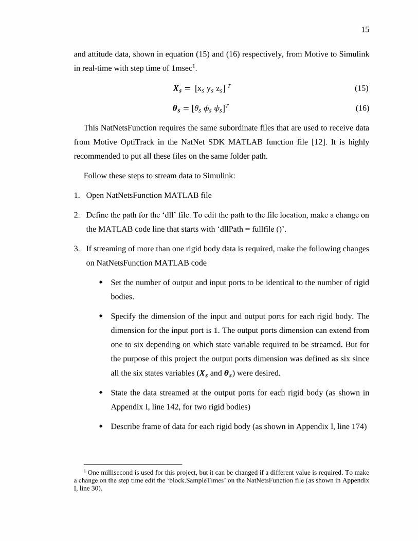
and attitude data, shown in equation (15) and (16) respectively, from Motive to Simulink

in real-time with step time of 1msec1.

𝑿𝒔 = [x𝑠 y𝑠 z𝑠] 𝑇 (15)

𝜽𝒔 = [𝜃𝑠 𝜙𝑠 𝜓𝑠]𝑇 (16)

This NatNetsFunction requires the same subordinate files that are used to receive data

from Motive OptiTrack in the NatNet SDK MATLAB function file [12]. It is highly

recommended to put all these files on the same folder path.

Follow these steps to stream data to Simulink:

1. Open NatNetsFunction MATLAB file

2. Define the path for the ‘dll’ file. To edit the path to the file location, make a change on

the MATLAB code line that starts with ‘dllPath = fullfile ()’.

3. If streaming of more than one rigid body data is required, make the following changes

on NatNetsFunction MATLAB code

Set the number of output and input ports to be identical to the number of rigid

bodies.

Specify the dimension of the input and output ports for each rigid body. The

dimension for the input port is 1. The output ports dimension can extend from

one to six depending on which state variable required to be streamed. But for

the purpose of this project the output ports dimension was defined as six since

all the six states variables (𝑿𝒔 and 𝜽𝒔) were desired.

State the data streamed at the output ports for each rigid body (as shown in

Appendix I, line 142, for two rigid bodies)

Describe frame of data for each rigid body (as shown in Appendix I, line 174)

1 One millisecond is used for this project, but it can be changed if a different value is required. To make

a change on the step time edit the ‘block.SampleTimes’ on the NatNetsFunction file (as shown in Appendix

I, line 30).

16

Define position and attitude data to be streamed for each rigid body (Appendix

I, line 178 to 185)

Define quaternion for each rigid body (Appendix I, line 187)

4. Open Motive OptiTrack

5. Follow the following steps to calibrate OptiTrack cameras and set an origin [13]

To calibrate:

Click on the layout tab found on the top left side of Motive window. Select

calibrate from the list shown under layout.

Click on the camera calibration pane and select a calibration type from the list

as shown below

Figure 8. Camera Calibration Pane

17

From the OptiWand section list, choose the correct calibration wand name

Click on start wanding

Start waving the Calibration wand, shown in Figure 9(a), across the entire

capture volume. Each of the cameras light turns to green when enough samples

are collected.

After enough samples are collected, all the cameras lights will turn to green,

click on the calculate button

Save the calibration file

Figure 9. (a) OptiTrack Calibration Wand (b) OptiTrack Calibration Square

To set the origin:

First place the calibration square, provided from OptiTrack, in the capture area

at a specific location, as shown in Figure 9(b).

Align the calibration square in a desired axis orientation

The long leg of the calibration square indicates the positive z-axis by default,

while the shorter leg indicates the x-axis. The positive y-axis is directed

upwards.

Next adjust the level indicator on the calibration square to balance the

calibration square

Open ground plane on Motive

a b

18

Set the vertical offset. The vertical offset is used to compensate the difference

between the actual ground plane and the center of markers on calibration square.

Click on the set ground plane tab

To further improve the leveling of the coordinate plane, place several markers

with a pre-known radius on the ground. Next, adjust the vertical offset for the

ground plane refinement with the marker’s radius. This function refines the

leveling using the marker's position.

Figure 10. Ground plane pane

6. Create a rigid body from markers as shown in Figure 11. In order to create a rigid body,

it is mandatory to link at least three markers together. Motive will automatically assign

the geometrical center for each rigid body created.

19

Figure 11. MCS cameras and Rigid body representation in Motive’s graphical

interface

7. Go to the view tab on the left side of Motive window and select data streaming pane

from the list to open the OptiTrack streaming engine.

8. Enable the broadcast frame data on OptiTrack streaming engine as shown in Figure 12

below.

9. Set the local interface to loopback if the streaming occurs in the same computer.

Otherwise, select the IP address of the computer in which the streaming should occur.

20

Figure 12. Data Streaming Engine Pane

10. Insert the IP address of the receiving computer on NatNetsFunction or set it to 127.0.0.1

if the same device is used (as shown in Appendix I, line 113).

11. Run the Simulink model corresponding with the NatNetsFunction to acquire the

streamed data on Simulink platform.

3.2. Controlling AR Drone from MATLAB-Simulink

The focus of this section of the thesis is to explain in detail the step required to

autonomously fly AR Drone using a Simulink-modelled control system. As described in

the previous section, NatNetsFunction was created with a level-2 s-function. A model

containing level-2 s-function requires a corresponding Target Language Compiler ‘TLC’

file to build it in Simulink and run it on a target hardware [14].

Two different models were created to address this shortcoming. In particular, these

models are

• OptiTrack model

• Controller model

21

The OptiTrack model ran the NatNetsFunction embedded model in ‘normal mode’

without the need to build it. The Controller model, on the other hand, can be built without

a separate TLC file because the model included in it is not created using a function

requiring the TLC file. It is therefore possible to build and run the controller model on the

target hardware. The two models will then share data in real time via Simulink Desktop

Real Time’s (SDRT) UDP communication.

3.2.1. OptiTrack Model

The OptiTrack model consists of the ‘From Motion Capture System’, ‘Trajectory

Generation’, ‘Controller Switch’ and ‘UDP Sender’. Each model is discussed below in

detail.

Figure 13. OptiTrack Model

a) From MCS:

This Simulink block is the embedded model of NatNetsFunction. As described in the

previous section, this block helps to extract the actual state of the drone from Motive

OptiTrack. In order to link the MATLAB s-function file to the Simulink model, the

following steps must be followed

Open s-function block from Simulink library browser.

Click on the function block

Write the NatNetsFunction name on the s-function name space.

22

b) Trajectory Generation:

The trajectory generation block is a reference path that is to be followed by the drone.

The output signal from the block is a vector 𝑿𝑐 which comprises of the commanded

position along the three coordinates axis and a yaw angle.

𝑿𝒄 = [x𝑐 y𝑐 z𝑐 𝜓𝑐] 𝑇 (17)

c) Controller Switch

The control switch is the manual switch which allows us to control the time of

transmission of the control data to the drone. By switching it on, the data from the controller

block can be transmitted to the drone while switching it off stops the process of sending

the data. This manual switch can always be switched on if you need to start sending control

data simultaneously with the start of the OptiTrack model.

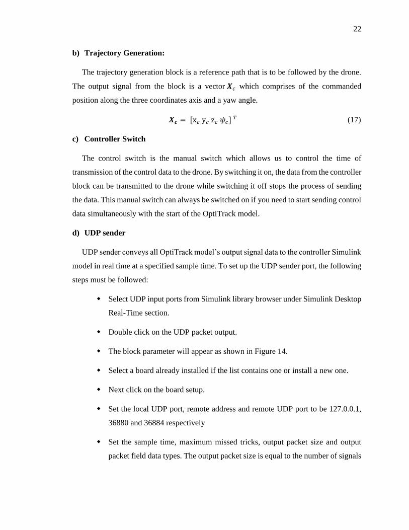
d) UDP sender

UDP sender conveys all OptiTrack model’s output signal data to the controller Simulink

model in real time at a specified sample time. To set up the UDP sender port, the following

steps must be followed:

Select UDP input ports from Simulink library browser under Simulink Desktop

Real-Time section.

Double click on the UDP packet output.

The block parameter will appear as shown in Figure 14.

Select a board already installed if the list contains one or install a new one.

Next click on the board setup.

Set the local UDP port, remote address and remote UDP port to be 127.0.0.1,

36880 and 36884 respectively

Set the sample time, maximum missed tricks, output packet size and output

packet field data types. The output packet size is equal to the number of signals

23

transferred multiply by eight. The maximum missed trick for the model is the

maximum number of missed data that is tolerated.

Figure 14. UDP Packet Output

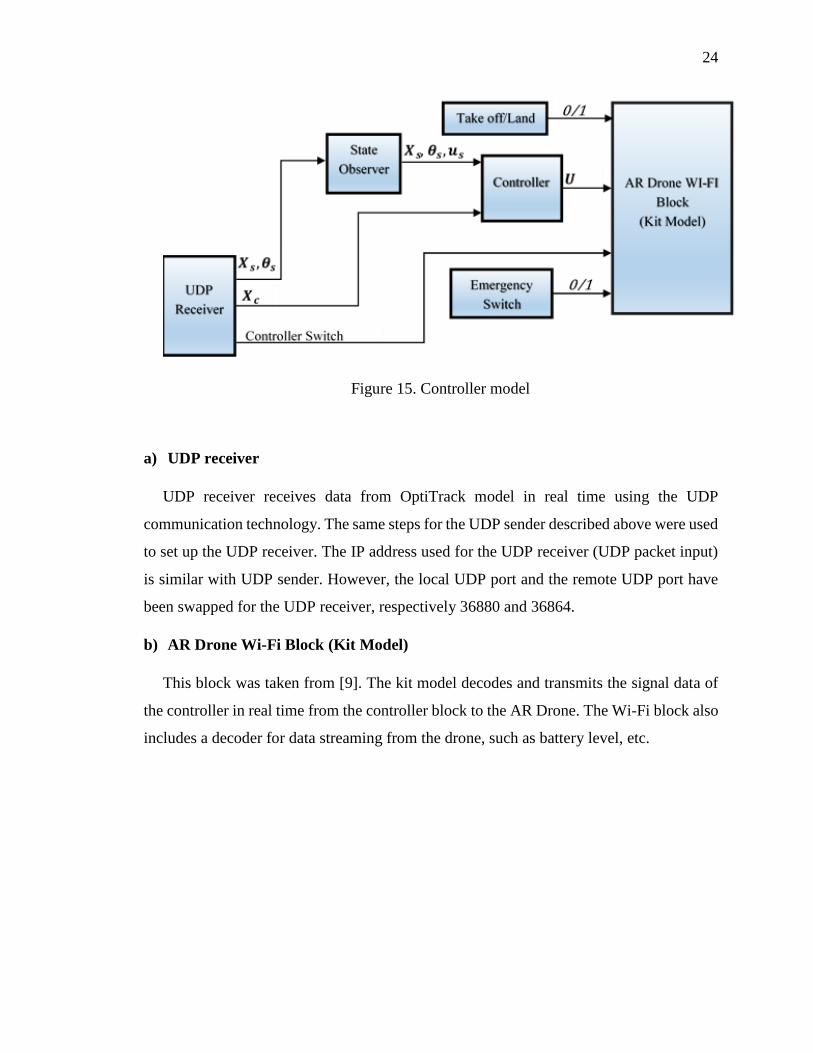
3.2.2. Controller Model

The controller model includes the AR Drone Wi-Fi block (kit model), state observer,

controller, UDP receiver and take off/land manual switch. This model runs in ‘external

mode’, allowing Simulink to communicate with the model deployed on the drone board

during runtime.

24

Figure 15. Controller model

a) UDP receiver

UDP receiver receives data from OptiTrack model in real time using the UDP

communication technology. The same steps for the UDP sender described above were used

to set up the UDP receiver. The IP address used for the UDP receiver (UDP packet input)

is similar with UDP sender. However, the local UDP port and the remote UDP port have

been swapped for the UDP receiver, respectively 36880 and 36864.

b) AR Drone Wi-Fi Block (Kit Model)

This block was taken from [9]. The kit model decodes and transmits the signal data of

the controller in real time from the controller block to the AR Drone. The Wi-Fi block also

includes a decoder for data streaming from the drone, such as battery level, etc.

25

Figure 16. AR Drone Wi-Fi block diagram

c) State Observer

State observer derives the body frame velocity 𝒖𝑠 from the components of the time

derivative of the position vector, ��𝑠 and the Euler angles, 𝜽𝑠 [4].

𝒖𝑠 = [𝑢 𝑣 𝑤]𝑇 (18)

��𝑠 = [x y z] 𝑇 (19)

𝜽𝑠 = [𝜃 𝜙 𝜓]𝑇 (20)

This block has three sets of output vectors: the current position 𝑿𝑠, the current attitude

angles 𝜽𝑠 and the body frame velocities 𝒖𝑠 vector. The body frame velocities are calculated

using the rotation matrix from equation (7) as follows.

[��] = [

𝑐𝑜𝑠𝜃𝑐𝑜𝑠𝜓 𝑠𝑖𝑛𝜙𝑠𝑖𝑛𝜃𝑐𝑜𝑠𝜓 − 𝑐𝑜𝑠𝜙𝑠𝑖𝑛𝜓 𝑐𝑜𝑠𝜙𝑠𝑖𝑛𝜃𝑐𝑜𝑠𝜓 + 𝑠𝑖𝑛𝜙𝑠𝑖𝑛𝜓𝑐𝑜𝑠𝜃𝑠𝑖𝑛𝜓 𝑐𝑜𝑠𝜙𝑐𝑜𝑠𝜓 + 𝑠𝑖𝑛𝜙𝑠𝑖𝑛𝜃𝑠𝑖𝑛𝜓 𝑐𝑜𝑠𝜙𝑠𝑖𝑛𝜃𝑠𝑖𝑛𝜓 − 𝑠𝑖𝑛𝜙𝑐𝑜𝑠𝜓

−𝑠𝑖𝑛𝜃 𝑠𝑖𝑛𝜙𝑐𝑜𝑠𝜃 𝑐𝑜𝑠𝜙𝑐𝑜𝑠𝜃] [

𝑢𝑣𝑤

]

(21)

26

d) Controller

A controller applies a responsive correction in order to provide an output that exhibit

the desired behavior using the feedback signals/state variables. A simple schematic

diagram below describes the functionality of a controller.

Figure 17. Schematic diagram of a feedback control system

As shown in the diagram above, the controller receives a difference between the

feedback signal and the reference value and sends a command signal to the plant. A

feedback data is then provided by a sensor that will be subtracted from the reference value

and sent to the controller to close the control system loop.

The kit model, which is used to transmit generated controller data to the target drone,

requires 𝑈z, 𝑈ψ, 𝑈𝜑 and 𝑈𝜃 as input variables. Therefore, a PID controller is used to

generate these four control variables. The 𝑼 control output vector is

𝑼 =

[ 𝑈𝜑

𝑈𝜃

𝑈ψ

𝑈z ]

(22)

As described in CHAPTER TWO, the forward movement, along the x-axis, and lateral

movement, along the y-axis, are controlled by generating pitch and roll angles,

respectively. As a result, the four control components are formulated, in PID fashion, as

follows [11]

𝑈�� = 𝐾𝑝,𝜓(𝜓𝑐 − 𝜓𝑠) + (𝜓𝑐 − 𝜓𝑠)𝐾𝑖,𝜓

𝑠 (23)

27

𝑈𝑧𝑑 = −𝐾𝑝,𝑧(𝑍𝑐 − 𝑍𝑠) − (𝑍𝑐 − 𝑍𝑠)𝐾𝑖,𝑧

𝑠 (24)

𝑈𝜃 = −𝐾𝑝,𝑡𝑥𝑒 − 𝐾𝑑,𝑡𝑉𝑥𝑒 − 𝐾𝑎𝑛𝑔𝑙𝑒𝑡𝜃𝑠 −𝐾𝑖,𝑡

𝑠𝑥𝑒 (25)

𝑈𝜙 = 𝐾𝑝,𝑓𝑦𝑒 + 𝐾𝑑,𝑓𝑉𝑦𝑒 + 𝐾𝑎𝑛𝑔𝑙𝑒𝑓𝜙𝑠 +𝐾𝑖,𝑓

𝑠𝑦𝑒 (26)

where,

𝐾𝑝,𝜓 and 𝐾𝑖,𝜓 are the proportional and integral gains for the yaw angle respectively.

𝜓𝑐 and 𝜓𝑠 are the commanded and actual values of yaw angle respectively.

𝐾𝑝,𝑧 and 𝐾𝑖,𝑧 are the proportional and integral gains for the altitude respectively.

𝑍𝑐 and 𝑍𝑠 are the commanded and actual values of the altitude respectively.

𝐾𝑝,𝑓, 𝐾𝑑,𝑓 and 𝐾𝑖,𝑓 are the proportional, derivation and integral gains for the roll angle

respectively.

𝐾𝑎𝑛𝑔𝑙𝑒𝑡 is a constant gain applied to minimize the controller error by subtracting a portion

of the feedback pitch angle.

𝐾𝑎𝑛𝑔𝑙𝑒𝑓 is a constant gain applied to minimize the controller error by subtracting a portion

of the feedback roll angle.

𝑦𝑒and 𝑉𝑦𝑒 are the position and velocity error in the y – axis.

𝜙𝑠 is actual value of the roll angle.

e) Take off/Land

This is a manual switch controlling the take-off and land command for a drone as the

name suggests.

The connection between AR. Drone 2.0 and ground station is established via Wi-Fi. A

modem/router or a USB Wi-Fi adapter can be used to create a connection with the AR

Drone network. For this project a USB Wi-Fi adapter was used.

28

To fly an AR Drone using the coordination of the two Simulink models, i.e. the

Controller model and OptiTrack model, the following steps must be followed:

1. First plug the USB adapter

2. Follow the necessary steps to set up the USB adapter

3. Connect your device (PC) with AR Drone network

4. Open the OptiTrack model and controller model

5. Make sure the NatNetsFunction is on the same path/folder as the rest of the files

6. Run ‘initial variables’ to reset all the variables such as the control gains (shown

in Appendix II)

7. Build the Controller model using ctrl + B or clicking the run button on Simulink

8. After the Controller model started running, run the OptiTrack model

9. Switch on the take-off/land to take off drone

10. Switch on the Controller switch (enable reference switch) to start sending the

controller data. Switching off the enable reference will stop the data sending

process

11. Switch off the take-off/land switch to land the Parrot

29

Figure 18. Overall Simulink diagram structure with MCS

30

CHAPTER FOUR

ACCURATE LANDING AND FORMATION

FLIGHT

As mentioned earlier, this chapter briefly discusses the two-benchmark multirotor GNC

problems. The first study tackled accurate landing guidance strategies. An emulated

autonomous battery recharging experiment was conducted using a mock-up battery

charging platform as a proof of concept for autonomous battery charging capability. Next,

the formation flight between two multirotors is studied. The main goal behind performing

the formation flight is to assess the accuracy of the controller to track, accurately, a desired

moving target position.

The idea and interest on autonomous charging robotics vehicles started mid-20th

century. As the applications of UAVs increased significantly, there is a rise in need of an

extended flight duration to accomplish a mission that requires a longer flight duration. To

address this problem, several research studies have now been carried out on an autonomous

charging system. In [15] researchers at the Massachusetts Institute of Technology were

able to perform autonomous landing and recharging of batteries of X-UFO and Draganflyer

drones using a recharging station.

Some researchers have worked with the Wireless Power Transfer (WPT) technique to

address this problem. WPT is a power transmission technology in which electrical energy

can be transmitted without a wire connection. In [16] and [17] WPT technology is used to

autonomously charge a multi-copter. The authors of [16] were able to wirelessly charge

AR Drone with an average WTP efficiency of 75%. One advantage of WTP is that it does

not require a very accurate approach to landing which makes it more valuable in this regard

than a docking strategy. The docking method, however, requires having an accurate control

system with a small error margin. Although the WTP reduces the need for a highly accurate

control system for the landing operation in contrast to the docking technique, it still faces

31

a great deal of drawback on their efficiency. The author in [16] calculated the WTP

efficiency as

𝐸 =𝑉0𝐼0

𝑉𝑖𝐼𝑖% (27)

where, 𝑉0 and 𝑉𝑖 are the output and input voltage while 𝐼0 and 𝐼𝑖 are the output and input

current.

In addition to the above research, authors of [18] used the cameras available on the

drone at the front and at the bottom to navigate through and make an autonomous landing.

Similarly, Carriera in [19] used a vision-based target localization to autonomously execute

landing operation. These papers, however, were not concerned with actually charging a

drone.

In the following sections, I will be describing the accurate landing strategies

implemented in ARTLAB.

4.1. Accurate Landing

A strategy is applied in this work to achieve an accurate drone landing. The first step in

the work of autonomously charging drones is to navigate where the charging platform is

located. Then, the drone tracks the position of a designated platform and lands on the

docking station safely and accurately.

The autonomous accurate landing of a drone is divided into the following three phases,

as shown in Figure 19.

Phase 1. Take-off

Phase 2. Closing

Phase 3. Landing/Docking

32

Figure 19. Three phases of accurate landing

4.1.1. Phase 1: Take-off

In this stage of the flight, the drone takes-off and hovers for a few seconds until the

controller command is initiated. AR Drones are equipped with autopilot system which

allows the aerial vehicles to have an autonomous take-off and hover in the air. For the

purpose of this paper, the duration time set for the drone to hover before the second phase,

i.e. closing phase, was 7 secs. Based on multiple experimental tests conducted, such

duration was found sufficient for the drone to take-off and had stabilized hovering.

4.1.2. Phase 2: Closing

In phase 2, the drone closes to the docking configuration following a predefined

trajectory. Such time trajectory was generated to control the speed at which the drone

approaches the last point. In particular, it is assumed that the trajectory components can be

described as fourth degree polynomials. The polynomial coefficients are calculated by

imposing the assigned initial and final conditions on position, and velocity and final

acceleration.

33

The general equation of the trajectory is given by,

𝑿(𝑡) = 𝑨𝟎 + 𝑨𝟏𝑡 + 𝑨𝟐𝑡2 + 𝑨𝟑𝑡

3 + 𝑨𝟒𝑡4 (28)

where, 𝑿 = [𝑥 𝑦 𝑧]𝑇 and 𝑨𝒊 = [𝑎𝑖 𝑏𝑖 𝑐𝑖]𝑇 with 𝑖 = 0,… ,4

As mentioned before, the coefficients 𝑨𝒊 are determined by imposing different boundary

conditions at initial2 time and final time. The exact position and speed of the drone at the

beginning of the closing phase or at the end of the take-off phase, which is taken from the

MCS, was therefore taken as the initial position and speed of the vehicle.

The final positions on the 𝑋 and 𝑌 axes were set to the 𝑋 and 𝑌 coordinates of the

landing platform respectively. The final altitude of the drone in the z coordinate axis was

set to be the height of the docking stage from the ground plus 0.15 meters. The reason for

the gap distance of 0.15 meters between the flying drone and the landing platform was to

allow the drone to hover and stabilize safely before landing. The disturbing ground effects

on the drone flight would increase dramatically at heights less than 0.15 meters. At the end

of the closing stage, the acceleration of the drone shall be equal to zero.

𝑿(𝑡0) = 𝑿𝟎 (29)

𝑿(𝑡𝑓) = 𝑿𝒇 (30)

��(𝑡𝑓) = 0 (31)

��(𝑡0) = ��𝟎 (32)

��(𝑡𝑓) = 𝟎 (33)

In turn, by setting the above boundary conditions and solving for the coefficients, these

unknown variables can be represented in terms of known parameters as follows.

2 Note that the time considered as initial here is the seventh second which is the end of the first phase and

the start of the second phase. Hence t means tc-ts, if tc is the current time and ts = 7sec.

34

For the x- axis coefficients:

Coefficients Expressions

𝑎0 𝑥0

𝑎1 ��0

𝑎2 −3(2𝑥0 − 2𝑥𝑓 + 𝑡𝑓��0)

𝑡2𝑓

𝑎3 8(𝑥0 − 𝑥𝑓) + 3𝑡𝑓��0

𝑡3𝑓

𝑎4 −(3𝑥0 − 3𝑥𝑓 + 𝑡𝑓��0)

𝑡4𝑓

Table 1 Expression for the coefficients of x- axis

For the y- axis coefficients:


𝑏0 𝑦0

𝑏1 𝑦𝑑0

𝑏2 −3(2𝑦0 − 2𝑦𝑓 + 𝑡𝑓��0)

𝑡2𝑓

𝑏3 8(𝑦0 − 𝑦𝑓) + 3𝑡𝑓��0

𝑡3𝑓

𝑏4 −(3𝑦0 − 3𝑦𝑓 + 𝑡𝑓��0)

𝑡4𝑓

Table 2 Expression for the coefficients of y- axis

35

For the z axis coefficients:


𝑐0 𝑧0

𝑐1 𝑧𝑑0

𝑐2 −3(2𝑧0 − 2𝑧𝑓 + 𝑡𝑓��0)

𝑡2𝑓

𝑐3 8(𝑧0 − 𝑧𝑓) + 3𝑡𝑓��0

𝑡3𝑓

𝑐4 −(3𝑧0 − 3𝑧𝑓 + 𝑡𝑓��0)

𝑡4𝑓

Table 3 Expression for the coefficients of z- axis

The total time duration required for the drone to complete the maneuver was calculated

based on the empirical observation that 𝑡 = 12.5 seconds is a reasonable amount of time

for the drone to cover 1 meter in translation. Based on the same assumption an average

velocity was calculated as

𝑉𝑎𝑣𝑔 =∆𝑠

∆𝑡= 0.08 𝑚/𝑠 (34)

Then, the time required for any specific flight could be retrieved by calculating the

distance from the initial to the final position and dividing it by the average velocity.

∆𝑡 =‖𝑿𝒇−𝑿𝟎‖

𝑉𝑎𝑣𝑔 (35)

4.1.3. Phase 3: Docking/Landing

Phase 3 is the last phase of the accurate landing. When the drone closes to the final

landing area, it must hover above the landing area until a docking configuration is achieved.

As described in the above section, the main goal of the accurate landing experimental

36

campaign is to dock on a mock-up landing stage. As shown in Figure 20, a set of wires

passes through the rectangular plate which connects to a LED. As the drone lands on the

platform, a cable placed underneath will close the circuit and the LED will light up to

demonstrate that it landed with the required accuracy.

Figure 20. Rectangular landing stage

In order to increase the landing accuracy and to boost the success rate, the drone’s

landing logic is established by extrapolating the current critical state variables for a correct

landing, namely distance to target and near zero speed. This approach allows to slightly

anticipate favorable landing condition instead of delaying the rotor shut-off to land off of

the docking stage. This theory is described in a Figure 21 below. Let assume the drone is

flying towards the green dot and presently it is at the blue dot position. If the drone position

is correctly extrapolated and predicted when the drone was at the blue point, the time it

took the drone to travel from the blue to the green point would make up for the time it took

the drone to meet the landing criteria and land safely. However, if the drone was made to

land when it arrived at the green point, the drone could be moved to the red dot point during

the time gap between meeting the logic and landing.

Wire LED Markers

37

Figure 21. Demonstration of why extrapolation was used

The extrapolation equation employed for the position vector X and velocity vector �� to

calculate the values at time 𝑡𝑖+1 is given by

𝑿(𝑡𝑖+1) = 𝑿(𝑡𝑖) +(𝑿(𝑡𝑖)−𝑿(𝑡𝑖−1))

𝑡𝑖−𝑡𝑖−1∗ 𝐾 (36)

��(𝑡𝑖+1) = ��(𝑡𝑖) +(��(𝑡𝑖)−��(𝑡𝑖−1))

𝑡𝑖−𝑡𝑖−1∗ 𝐾 (37)

where, 𝑡𝑖−1 and 𝑡𝑖 are the previous and present time instants respectively and K is a

compensation constant to be tuned during the experimental campaign.

By changing the constant K, the extrapolation values which gave a satisfactory result

are adjusted. A separate logic was applied independently for the planar and the vertical

motion. Changing the variables, values that gave a decent result were determined.

(𝑥(𝑡𝑖+1) − 𝑥𝑐)2 < 휀𝑥

2 (38)

(𝑦(𝑡𝑖+1) − 𝑦𝑐)2 < 휀𝑦

2 (39)

𝑧(𝑡𝑖+1) < 𝑧𝑐 + 휀𝑧 (40)

��(𝑡𝑖+1)2 + ��(𝑡𝑖+1)

2 < 휀��2 (41)

��(𝑡𝑖+1) < 휀�� (42)

where,

• 𝑥𝑐, 𝑦𝑐 and 𝑧𝑐 are the commanded values

38

• 𝑥, 𝑦, 𝑧 and ��, ��, �� are the position and velocity at 𝑡𝑖+1on the 𝑥, 𝑦 and 𝑧 coordinates.

• 휀𝑥, 휀𝑦 and 휀𝑧 are the error tolerated for the position in each three coordinates.

• ε�� and εz are the error tolerated for the velocity.

Tests proved that satisfactory results are achieved with

K 휀𝑥 휀𝑦 휀𝑧 휀�� 휀��

0.2 0.03 0.03 0.05 0.04 0.05

Table 4 Accurate landing values

Figure 22 below shows the commanded and actual trajectory for the three coordinates

and the yaw angle. It is important to note that the initial seven seconds of the maneuver are

actually used to perform the take-off. The actual commanded trajectory begins right after

the seventh second. As described in the previous section, this is the duration of time set

until the control data allowed to be streamed.

Figure 22. Position plot on the x, y and z and yaw angle plot

The 3D plot of the trajectory is shown in the following Figure 23.

39

Figure 23. 3D plot of the accurate landing path

The histories of the control variables, 𝑈��, 𝑈𝜃 and 𝑈𝜑, and the histories of actual vertical

velocity, pitch and roll angles, are reported in Figure 24 below.

When I have introduced the OptiTrack and controller model in section 3.2.2, it was

stated that the controller model should run first before the OptiTrack model. This procedure

is reflected into a time gap shown in the Figure 24 below. In other words, it is the time lost

before the OptiTrack model data begins to be sent to the controller model, which was

caused by the time it took to run and compile the OptiTrack model3 and the drones to start

flying.

3 OptiTrack model is run and compiled after the controller model was run and compiled

40

Figure 24. The control outputs plot versus their feedback values

4.2. Formation Flight

Another topic in this thesis paper is the autonomous formation flight of two mutirotors.

Different research groups worked on drone coordination flight for multiple drones to

accomplish different and articulated tasks, such as rescue operation, structures inspection,

fire control missions, etc.

In this paper, with the main objective of testing the accuracy of the controller, two are

requested to execute a formation flight to achieve a steady alignment. To perform such

maneuver the two vehicles will behave simultaneously as target and chaser. As shown in

the following Figure 25, the two drones start in two different positions, drone 1 from P1_o

and drone 2 from P2_o. After takeoff each vehicle will start to chase the other vehicle and

reach the final points of P1f and P2f. The two final points of the drones separated by a

constant value of 2D in the 𝑋 axis.

41

Figure 25. Hovering of two drones in a coordination flight

One of the challenges faced in the coordination of the two drones was that the drones

continued to fly together instead of stabilizing and hovering together at a point fixed to the

absolute frame of reference. As a result, the two vehicles will be prone to simultaneously

drift toward some direction. Various techniques were used to tackle this problem. The one

that delivered satisfactory results is discussed here.

For each coordinate, a simple equation was used in which each drone target position is

the sum of its current position plus a portion of the relative position with respect to the

other vehicle so that the gap between them continues to be minimized and converge toward

the final assigned distance 2D. This can be further illustrated on the 𝑥 − 𝑦 plane in the

Figure 26 below. The first drone moves from the blue dot to the black dot position adding

a percentage of the difference between the initial position of the first and second drone. At

the same time, the second drone also adds a percentage of the distance between the first

positions of the two drones to reach at the black dot position. This process continues until

both drones reach at the same point.

42

Figure 26. Illustration of coordination equation used

The illustration above can be mathematically described as follow. Let 𝑑𝑡 be the

maneuver time interval, then the target location of drone 1 is

𝑥1(𝑡 + 𝑑𝑡) = (𝑥2(𝑡) − 𝑥1(𝑡))𝑘𝑥 + 𝑥1(𝑡) − 𝐷 (43)

𝑦1(𝑡 + 𝑑𝑡) = (𝑦2(𝑡) − 𝑦1(𝑡))𝑘𝑦 + 𝑦1(𝑡) (44)

𝑧1(𝑡 + 𝑑𝑡) = (𝑧2(𝑡) − 𝑧1(𝑡))𝑘𝑧 + 𝑧1(𝑡) (45)

Similarly, for the second drone

𝑥2(𝑡 + 𝑑𝑡) = (𝑥1(𝑡) − 𝑥2(𝑡))𝑘𝑥 + 𝑥2(𝑡) + 𝐷 (46)

𝑦2(𝑡 + 𝑑𝑡) = (𝑦1(𝑡) − 𝑦2(𝑡))𝑘𝑦 + 𝑦2(𝑡) (47)

𝑧2(𝑡 + 𝑑𝑡) = (𝑧1(𝑡) − 𝑧2(𝑡))𝑘𝑧 + 𝑧2(𝑡) (48)

As mentioned above, the value of 𝑥, 𝑦 and 𝑧 values at (𝑡 + 𝑑𝑡) is the current position

of either drone plus a constant (𝑘𝑥 or 𝑘𝑦 or 𝑘𝑧) multiplying the difference between the two

drones. The constants 𝑘𝑥, 𝑘𝑦 and 𝑘𝑧 are compensation constants for the components 𝑥, 𝑦

and 𝑧, respectively, which can be tuned experimentally to achieve satisfactory

performances.

Based on experimental campaign results the following values have been selected

43

𝑘𝑧 𝑘𝑦 𝑘𝑥 𝐷 [𝑚]

0.7 0.4 0.4 0.6

Table 5 Formation flight results

In Figure 27 are shown the results for the formation flight in each axis. In particular, the

three figures report the commanded and actual position component histories for both

drones. Separately, the time histories of the position components are represented in Figure

28. Similarly, the plots for the second drone are shown in Figure 29.

Figure 27. Formation flight plot

44

Figure 28. Drone 1 plot in the x, y and z direction

Figure 29. Drone 2 plot in the x, y and z direction

45

CHAPTER FIVE

COMPARISON OF NLP SOLVERS

In the last decades, there has been a growing interest towards fast numerical methods to

solve nonlinear programming problems (NLP), namely, to find the minimum of a scalar

function 𝑓(𝑥) subject to a constraint ∅(𝑥) = 0 [20]. This particular interest reflects into a

growing demand of advanced NLP solver methods capable of solving large-scale

optimization problems. A variety of nonlinear programming solvers are currently available

to address optimization problems, including ARTELYS KNITRO, IPOPT, MIDACO,

Dlib, MATLAB-FMINCON, and SGRA.

Several of these NLP solvers are commercial products and are hardly available online

as free source software. However, there are a few that can be easily downloaded. Some

have a free trial version for a specific time allotment. The software for NLP solvers is often

written in popular computer programming languages such as C or Python. A few of the

software can be integrated and executed in MATLAB as well.

In this paper the performance of Sequential Gradient-Restoration Algorithm (SGRA)

was compared with a variety of other NLP solvers that can be executed in MATLAB. The

testing was based on performance comparison using various benchmark problems. There

are very few research publications that worked on a similar topic. In [20] the author

compares the properties of multiple algorithms based on their computational time and

ability to converge to the solution using 16 numerical examples as a test problem.

Similarly, using benchmark problems containing as many as twenty variables, the

performance of eight different optimization methods were evaluated in [21]. However, in

that particular paper the optimization method discussed are applied to unconstrained

optimization problems.

Six different NLP solvers were considered in this thesis based on online availability and

MATLAB compatibility. The comparison was done using a collection of 13 different

benchmark test problems retrieved from [20] and [22]. The comparison was then based on

46

the reliability and efficiency of each solver, measured by the time the calculation took to

reach a certain level of precision.

5.1. Problem Statement

Nonlinear programming is a particular branch of optimal control theory and it is based

on the minimization of a scalar objective function subjected to a set of inequality

constraints. The general form of nonlinear programming problem can be stated as:

Min 𝑓 = 𝑓(𝒙) (49)

subject to:

(𝒙) ≥ 0

with 𝑓: 𝑅𝑛 → 𝑅 and : 𝑅𝑛 → 𝑅𝑞 nonlinear functions and 𝑛 > 𝑞, for a bonafide

optimization problem. The vector 𝒙 = (𝑥1, 𝑥2, … , 𝑥𝑛)𝑇 contains all the optimization

variables.

5.2. Nonlinear Programming Solver

As mentioned in the first part of this chapter, there are many commercially available

NLP solvers. Nevertheless, only a few can be freely downloaded and used. In addition, not

all of them supports MATLAB which is a software platform used in this paper to run the

NLP optimization approaches.

The NLP solvers discussed in this paper are listed below.

I. SGRA (Sequential Gradient-Restoration Algorithm) is a nonlinear programming

solver algorithm composed of a sequence of gradient phases and restoration phases.

I coded SGRA using MATLAB software.

II. ARTELYS KNITRO4 is a commercially available software package for solving

nonlinear optimization problems that has developed since 2001 by Zienna

4 Since the trial version of this software was used in this paper the performance might be different than

the full version

47

Optimization. The solver name KNITRO is a short form for ‘nonlinear interior

point trust region optimization’. KNITRO has presented an interface to use the

software in MATLAB. KNITRO can be used using two different algorithms.

a. Interior-point (IP)

b. Active-set (AS)

The trial version of the software is used in this paper.

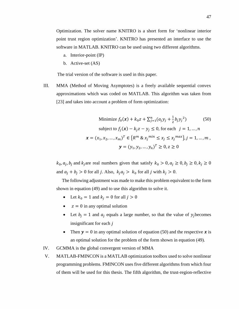
III. MMA (Method of Moving Asymptotes) is a freely available sequential convex

approximations which was coded on MATLAB. This algorithm was taken from

[23] and takes into account a problem of form optimization:

Minimize 𝑓0(𝒙) + 𝑘0𝑧 + ∑ (𝑎𝑗𝑦𝑗 +1

2𝑏𝑗𝑦𝑗

2)𝑛𝑗=1 (50)

subject to 𝑓𝑗(𝒙) − 𝑘𝑗𝑧 − 𝑦𝑗 ≤ 0, for each 𝑗 = 1,… , 𝑛

𝒙 = (𝑥1, 𝑥2, … , 𝑥𝑚)𝑇 ∈ {𝑅𝑚 & 𝑥𝑗𝑚𝑖𝑛 ≤ 𝑥𝑗 ≤ 𝑥𝑗

𝑚𝑎𝑥}, 𝑗 = 1,… ,𝑚 ,

𝒚 = (𝑦1, 𝑦2, … , 𝑦𝑛)𝑇 ≥ 0, 𝑧 ≥ 0

𝑘0, 𝑎𝑗 , 𝑏𝑗 and 𝑘𝑗are real numbers given that satisfy 𝑘0 > 0, 𝑎𝑗 ≥ 0, 𝑏𝑗 ≥ 0, 𝑘𝑗 ≥ 0

and 𝑎𝑗 + 𝑏𝑗 > 0 for all 𝑗. Also, 𝑘𝑗𝑎𝑗 > 𝑘0 for all 𝑗 with 𝑘𝑗 > 0.

The following adjustment was made to make this problem equivalent to the form

shown in equation (49) and to use this algorithm to solve it.

• Let 𝑘0 = 1 and 𝑘𝑗 = 0 for all 𝑗 > 0

• 𝑧 = 0 in any optimal solution

• Let 𝑏𝑗 = 1 and 𝑎𝑗 equals a large number, so that the value of 𝑦𝑗becomes

insignificant for each 𝑗

• Then 𝒚 = 0 in any optimal solution of equation (50) and the respective 𝒙 is

an optimal solution for the problem of the form shown in equation (49).

IV. GCMMA is the global convergent version of MMA

V. MATLAB-FMINCON is a MATLAB optimization toolbox used to solve nonlinear

programming problems. FMINCON uses five different algorithms from which four

of them will be used for this thesis. The fifth algorithm, the trust-region-reflective

48

algorithm, requires bound or linear equality constraints, and since the example

problems in this paper contain non-linear constraints, the trust-region-reflective

algorithm has been excluded from this research. The four algorithms used are listed

below

a. Interior-point (IP)

b. Sequential quadratic programming (SQP)

c. Sequential quadratic programming -legacy (SQPL)

d. Active-set (AS)

VI. MIDACO5 (Mixed Integer Distributed Ant Colony Optimization) is an

optimization solver which is based on the ant colony optimization algorithm. The

trial version of MIDACO that only works with a maximum of four variables

problem was used in this paper.

Of these NLP solvers I, III, IV and VI requires the gradient of the objective function

and the constraints. No gradient function is required for the rest. To solve an

optimization problem, MMA and GCMMA always need a lower and upper bound of

the variable.

5.3. Example Problems and Result

Thirteen different problems are studied to compare the solver performance. The

variables number n ranges from two to twelve. Similarly, the number of constraints q varies

from one to four. Information about each solver performance is tabulated following the

expression for each problem. The CPU times shown in the tables are the average value of

three consecutive simulation run.

5 Since the trial version of this software was used in this paper the performance might be different than

the full version

49

Problem 1:

Min 𝑓(𝑥) = 𝑥12 + 𝑥2

2 + 𝑥32 + 𝑥4

2 + 𝑥52 + 𝑥6

2 + 𝑥72 + 𝑥8

2 + 𝑥92 + 𝑥10

2 + 𝑥112 +

𝑥122 (51)

subject to the constraints:

∅1(𝑥) = 𝑥1 + 𝑥3𝑥2 − 1

∅2(𝑥) = 𝑥2 + 𝑥5 − 2𝑥7

∅3(𝑥) = 𝑥8 + 𝑥4 − 𝑥9 + 3

∅4(𝑥) = 𝑥10 + 𝑥11 + 𝑥12 − 1

With initial guess of 𝑥 = 𝑜𝑛𝑒𝑠(12,1), the calculation time and final and the initial

function value for each of the solvers is tabulated below.

Initial guess 𝑥 = 𝑜𝑛𝑒𝑠(12,1)

Name Initial

function value

Final

function value

CPU time

FMINCON SQP

12

4.3333

0.2520

SQP-legacy 0.276

Active-set 0.2796

Interior-point 0.4267

SGRA 4.3335 0.0099

KNITRO Interior-point 4.3333 0.0512

Active-set 0.1489

MMA 4.383 49.3021

GCMMA 4.3819 29.023223

Table 6 Comparison of solvers using problem 1

From the table above SGRA converges, with a calculation time of 0.0099 sec, faster

than the rest of the optimization approaches. MMA and GCMMA didn’t converge to the

optimal solution and as number of iterations for increased the solution even diverges further

from the optimal solution.

50

Problem 2:

Min 𝑓(𝑥) = −𝑥1𝑥2𝑥3𝑥4 (52)


∅1(𝑥) = 𝑥13 + 𝑥2

2 − 1

∅2(𝑥) = 𝑥12 + 𝑥4 − 𝑥3

∅3(𝑥) = 𝑥42 − 𝑥2


Name Initial

function value

Final

function value

CPU time

FMINCON SQP

-1

-0.25

0.137303

SQP-legacy 0.2456

Active-set 0.275


SGRA 0.0017

KNITRO Interior-point 0.0375

Active-set 0.0358

MMA 1.4054

GCMMA 3.9768

MIDACO -0.249 9.7018


From the table above for the benchmark problem 2, the SGRA still converges faster

than the rest of the solvers with a CPU time of 0.0017 sec. For KNITRO, however, the AS

algorithm has a smaller benefit in CPU time than the internal point algorithm in this unlike

problem 1.

51

Problem 3:

Min 𝑓(𝑥) = (𝑥1 − 1)2 + (𝑥2 − 2)2 + (𝑥3 − 3)2 + (𝑥4 − 4)2 (53)


∅1(𝑥) = 𝑥1 − 2

∅2(𝑥) = 𝑥32 + 𝑥4

2 − 2


Name Initial

function value

Final

function value

CPU time

FMINCON SQP

14

13.8579

0.134257

SQP-legacy 0.2559

Active-set 0.2761


SGRA 13.8579 0.0074


Active-set 0.0369

MMA 13.8588 0.3509

GCMMA 13.8579 9.4765

MIDACO 13.8534 8.2057


MMA solves the problem faster than the FMINCON-IP algorithm. FMINCON,

however, solved the problem without applying the upper and lower limits, while MMA

needs the upper and lower limits to solve the problem.

52

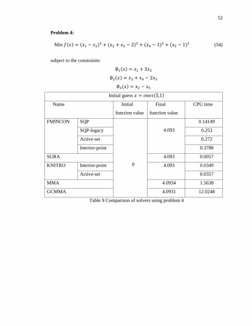
Problem 4:

Min 𝑓(𝑥) = (𝑥1 − 𝑥2)2 + (𝑥2 + 𝑥3 − 2)2 + (𝑥4 − 1)2 + (𝑥5 − 1)2 (54)


∅1(𝑥) = 𝑥1 + 3𝑥2

∅2(𝑥) = 𝑥3 + 𝑥4 − 2𝑥5

∅3(𝑥) = 𝑥2 − 𝑥5


Name Initial

function value

Final

function value

CPU time

FMINCON SQP

0

4.093

0.14149

SQP-legacy 0.253

Active-set 0.272


SGRA 4.093 0.0057


Active-set 0.0357

MMA 4.0934 1.5638

GCMMA 4.0931 12.0248


53

Problem 5:

Min 𝑓(𝑥) = (𝑥1 − 1)2 + (𝑥1 − 𝑥2)2 + (𝑥2 − 𝑥3)

4 (55)


∅1(𝑥) = 𝑥1(𝑥22 + 1) + 𝑥3

4 − 4 − 3√2


Name Initial

function value

Final

function value

CPU time

FMINCON SQP

0

0.0326

0.14154

SQP-legacy 0.2504

Active-set 0.2686


SGRA 0.0326 0.007


Active-set 0.0366

MMA 0.0334 8.9878

GCMMA 0.0344 818.5

MIDACO 0.0326 2.1517


If either the lower or the upper bound were not applied, MIDACO would not converge

to the optimum solution for the above problem. In the table above, a lower limit of zero is

used for solving the problem by MIDACO which converged more quickly than MMA.

54

Problem 6:

Min 𝑓(𝑥) = (𝑥1 − 1)2 + (𝑥1 − 𝑥2)2 + (𝑥3 − 1)2 + (𝑥4 − 1)4 + (𝑥5 − 1)6 (56)


∅1(𝑥) = 𝑥12𝑥4 + sin(𝑥4 − 𝑥5) − 2√2

∅2(𝑥) = 𝑥2 + 𝑥34𝑥4

2 − 8 − √2


Name Initial function

value

Final

function value

CPU time

FMINCON SQP

0

0.2415

0.154386

SQP-legacy 0.2627

Active-set 0.2821


SGRA 0.2415 0.0031


Active-set 0.0366

MMA 0.3974 76.7057

GCMMA 0.4337 238.1397


MMA and GCMMA displayed a disagreement from the optimal solution while the other

solvers calculated the solution with the same trend observed for the other problems.

55

Problem 7:

Min 𝑓(𝑥) = (𝑥1 − 1)2 + (𝑥1 − 𝑥2)2 + (𝑥2 − 𝑥3)

2 + (𝑥3 − 𝑥4)4 + (𝑥4 − 𝑥5)

4 (57)


∅1(𝑥) = 𝑥1 + 𝑥22 + 𝑥3

2 − 2 − 3√2

∅2(𝑥) = 𝑥2 − 𝑥32 + 𝑥4 + 2 − 2√2

∅3(𝑥) = 𝑥1 + 𝑥5 − 2



value

Final function

value

CPU time

FMINCON SQP

0

0.1623

0.142924

SQP-legacy 0.2543

Active-set 0.284


SGRA 0.1623 0.0087


Active-set 0.0398

MMA 0.1623 12.26

GCMMA 0.1623 202.165


56

Problem 8:

Min 𝑓(𝑥) = 0.01(𝑥1 − 1)2 + (𝑥2 − 𝑥12)2 (58)


∅1(𝑥) = 𝑥1 + 𝑥32 + 1


Name Initial

function value

Final function

value

CPU time

FMINCON SQP

0

0.0404

0.140382

SQP-legacy 0.2707

Active-set 0.2897


SGRA 0.0404 0.0156


Active-set 0.0408

MMA 0.0425 0.2453

GCMMA 0.0401 2.7936

MIDACO 0.041411 1.2939


57

Problem 9:

Min 𝑓(𝑥) = −𝑥1 (59)


∅1(𝑥) = 𝑥2 − 𝑥13 − 𝑥3

2

∅2(𝑥) = 𝑥12 − 𝑥2 − 𝑥4

2


Name Initial

function value

Final function

value

CPU time

FMINCON SQP

-1

-1 0.141759

SQP-legacy 0.2562

Active-set -1.0622 0.3241

Interior-point -1 0.3838

SGRA -1 0.0105

KNITRO Interior-point -1 0.0355

Active-set 0.0378

MMA -1 1.3648

GCMMA -1 238.3986

MIDACO -0.97989 4.9125


58

Problem 10:

Min 𝑓(𝑥) = log(1 + 𝑥12) − 𝑥2 (60)


∅1(𝑥) = (1 + 𝑥12)2 + 𝑥2

2 − 4

Initial guess 𝑥 = 𝑧𝑒𝑟𝑜𝑠(2,1) + 2


value

Final function

value

CPU time

FMINCON SQP

-0.3906

-1.7321

0.141832

SQP-legacy 0.2482

Active-set 0.2665

Interior-point 0.43

SGRA -1.7321 0.012776

KNITRO Interior-point -1.7321 0.0406

Active-set 0.0345

MMA -1.7321 1.0169

GCMMA -1.7325 790.7121

MIDACO -1.7322 0.1757


59

Problem 11:

Min 𝑓(𝑥) = (𝑥1 − 20)2 + (𝑥2 + 20)2 (61)


∅1(𝑥) = (𝑥1

𝑎)2 + (

𝑥2

𝑏)2 − 1

𝑎 = 10; 𝑏 = 10

Initial guess 𝑥 = [4,−5]

Name Initial

function value

Final function

value

CPU time

FMINCON SQP

481

334.3146

0.140921

SQP-legacy 0.2389

Active-set 0.2552


SGRA 334.3146 0.007402


Active-set 0.037

MMA 334.3146 0.0802

GCMMA 334.3146 0.3817

MIDACO 334.3146 0.7344


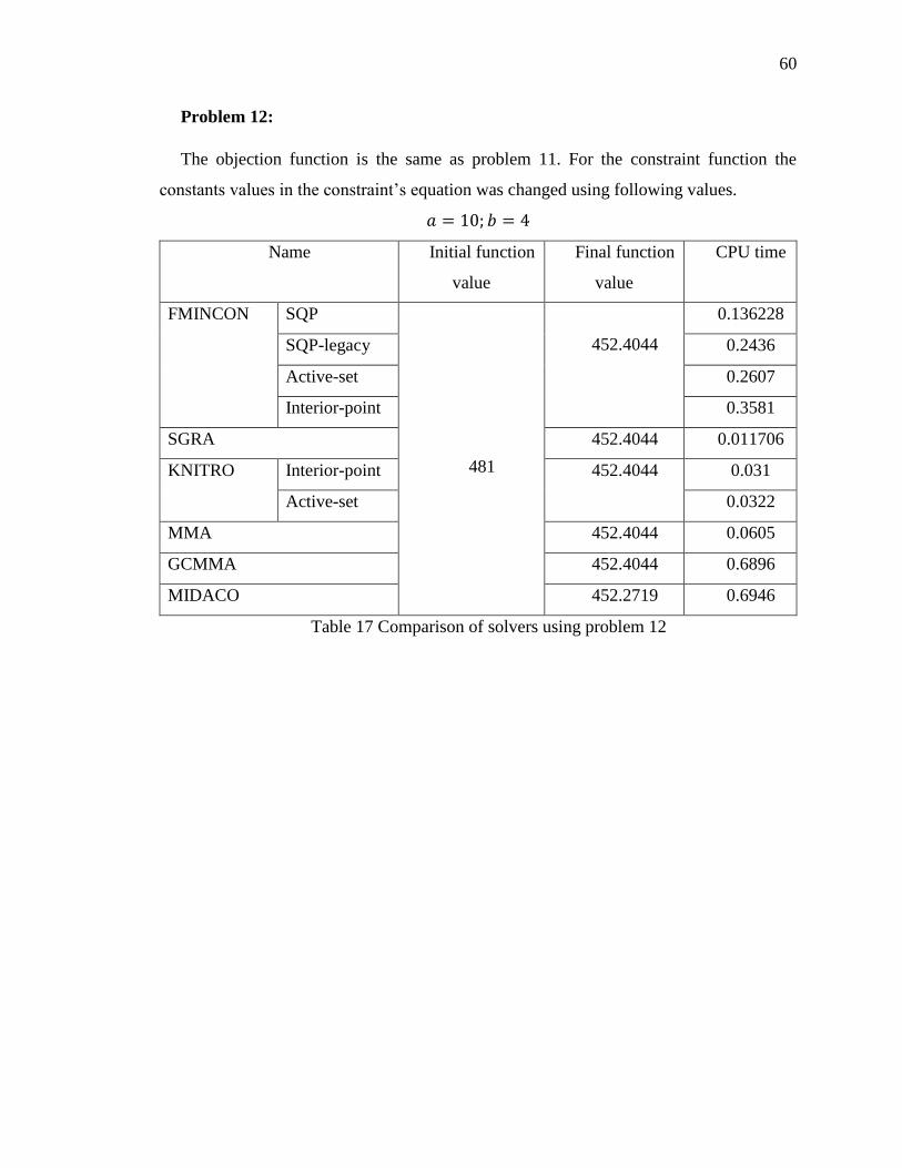
60

Problem 12:

The objection function is the same as problem 11. For the constraint function the

constants values in the constraint’s equation was changed using following values.

𝑎 = 10; 𝑏 = 4


value

Final function

value

CPU time

FMINCON SQP

481

452.4044

0.136228

SQP-legacy 0.2436

Active-set 0.2607


SGRA 452.4044 0.011706


Active-set 0.0322

MMA 452.4044 0.0605

GCMMA 452.4044 0.6896

MIDACO 452.2719 0.6946


61

Problem 13:

Similarly, for problem 13, the same objection and constraint function as problem 11 was

used with constraint equation constants of,

𝑎 = 10; 𝑏 = 1

Name Initial

function value

Final function

value

CPU time

FMINCON SQP

617

496.1121

0.142002

SQP-legacy 0.2471

Active-set 0.2616


SGRA 496.1121 0.012376


Active-set 0.0356

MMA 496.1124 0.1584

GCMMA 496.1124 1.7066

MIDACO 496.0119 0.6306


Of the methods implemented to solve NLP problems, SGRA was the most consistent

and efficient from the tabulated results of 13 different example problems. This algorithm

has proven to be a very powerful solver by completing all the problems in a much smaller

calculation time. The ARTELY KNITRO method had a higher calculation time than

SGRA. However, despite that, it performed better than the rest of the methods, for both the

interior-point and active set algorithm. In some examples MMA performed better than the

algorithms used by FMINCON but considering the consistency and the ability to use

FMINCON without the need for upper and lower bound as well as a gradient function, it

can be concluded that FMINCON is more efficient and reliable than MMA, GCMMA and

MIDACO.

62

CHAPTER SIX

TRAJECTORY OPTIMIZATION

Trajectory generation for multirotors is based on the construction of a set of space points

that describe the transfer path of the vehicle from an initial position to a final position. In

general, a particular criterion must be selected to generate a desired trajectory. For

example, in section 4.1, I have used polynomial expressions to describe the trajectory

components that transfer the vehicle from its initial position to a desired final position. The

coefficients of these polynomials were chosen so to satisfy the boundary conditions on

position, velocity, and acceleration. In this section, I will be describing a trajectory

generation strategy that aims to address the limited flight duration of a multirotor. In

particular, I will investigate optimal trajectories which minimize the energy required by a

multirotor to transfer from its current position to a final position within a given time.

With this goal in mind, the maneuver energy optimization is achieved through the

minimization of jerk J, which is the rate of change of acceleration.

𝐽 =𝑑𝑎

𝑑𝑡= (

𝑑𝐹

𝑑𝑡)/𝑚 (62)

providing that the body mass 𝑚 is constant.

A work from Mueller et.al. [24], proved that minimizing the control effort on a

quadrotor is equivalent to minimizing the manoeuvre jerk. In particular, the authors proved

that minimizing the jerk is equivalent to minimizing the upper bound of the product of the

control inputs (total thrust and body angular rates).

∫ (𝑓(𝑡)2‖𝜔(𝑡)‖2)𝑑𝑡𝑇

0≤ ∑ 𝐽𝑖

3𝑖=1 (63)

where J is the jerk, 𝑓 is the total thrust, 𝑖 is the axis subscript and 𝜔 is the body angular rate

Hence minimizing the jerk would minimize the product of the control inputs. The

control inputs, however, are the major force that consume the power energy of the drone.

63

Consequently, minimizing these control inputs will also reduce the power consumption.

As a result, the jerk minimization reflects into minimizing the power consumption.

6.1. Previous Works

A number of solutions to enhance endurance have recently been proposed in the

literature. Most of these projects focused on improving the mechanical design and power

systems, whereas other research teams developed a minimum energy path guidance

strategy. In [25], MIT researchers proposed a hardware platform for a battery swamp

strategy that enables UAVs to autonomously swamp batteries and perform a long–duration

task. In a similar context, Ure et.al. developed an automatic system in [26] that can switch

drained batteries with a charged battery while recharging several other batteries

simultaneously. Another group of researchers in [27] attempted to address the endurance

performance of electrically powered UAVs by dumping batteries that were depleted. This

can, however, raise concerns about environmental pollution and safety issues.

In addition to those studies that attempted to solve the endurance limitations of UAVs

by improving the power system, several other studies have also been carried out to improve

the mechanical design of UAVs. One example of these projects is reported in [28], where

Gurdan et.al. created a low-weight flying robot that is energy efficient. Furthermore, the

authors in [29] described a new energy efficient rotor configuration for a quadrotor.

The generation of an energy-optimal trajectory to deal with the problem of energy

consumption received some attention in the rotorcraft literature only in recent years. Yacef

et. al. in [30] proposed an optimal control problem using an energetic model to optimize

the UAV’s trajectory which minimizes the consumption of energy. In that work, a NLP

solver software called GPOPS-II was used to solve the proposed optimal control offline.

Similarly, in [1] the author, by leveraging electrical model of a brushless DC motor,

determined minimum energy trajectory using ACADO Toolkit to solve optimal control

problem for DJI Phantom 2. The solver took more than 65 sec in average to calculate the

optimal solution as stated in the same paper, which hinders the ability to apply it in real-

time. This forced the author to solve optimal problem offline and deploy the trajectory.

There have been also researchers, such as in [31], who introduced a software system by the

64

name of Green Flight that can acquire battery data during a mission and make suggestions

on how to optimize the consumption. Although this software system approach is quite

different than generating trajectory that would minimize energy, it would give the user the

ability to decide what to do based on the battery energy analysis delivered by the system.

The guidance strategy addressed by multiple researchers on this topic showed that they

executed the optimization calculation offline and deploy the trajectory afterwards.

However, in real environmental situations, it would be difficult to achieve optimal value

as the environment highly affect the trajectory. Hence, working towards real-time

optimization is the preferable approach. In this thesis real time guidance strategy for

minimum energy is introduced.

6.2. Bezier Curve

Bezier curve is a particular parametric curve between two end points. This curve had its

initial applications in computer graphics and related fields. It is also practical in mechanical

and electrical engineering applications. An example of a quadratic Bezier curve is shown

in Figure 30 below. P0 and P2 are the end points of the Bezier curve while P1 is the control

point.

Figure 30. Quadratic Bezier curve

Lately, there have been a growing interest in the use of Bernstein polynomials for aerial

vehicle trajectory generation. In the work of Cichella et.al. [32], a Bernstein approximation

was used to propose a minimum jerk optimal trajectory for a differentially flat aerial

65

vehicle. That paper presents a collision avoidance trajectory generation system using

MATLAB FMINCON as NLP solver. Notably, the NLP problem was derived from the

original optimal control problem formulated to achieve the collision avoidance mission

while minimizing the jerk. The fundamental equations discussed on that paper are reported

in the following section. For further detailed mathematical derivation it is recommended to

refer to [32].

A Bezier curve function can be defined as the summation of a control points multiplied

by the Bernstein polynomial.

𝐵𝑛(𝑡) = ∑ 𝑐𝑖𝑝𝑖,𝑛(𝑡)𝑛𝑖 (64)

where 𝑛 is the Bernstein polynomial degree, 𝑐𝑖 are control points (𝑖 = 0, 1, … , 𝑛), and the

polynomial

𝑝𝑖,𝑛(𝑡) =(𝑛

𝑖 )(𝑡𝑓−𝑡)𝑛−𝑖

𝑡𝑖

𝑡𝑖𝑛 (65)

is known as the Bernstein polynomial of degree 𝑛.

The set of all 𝑖 combination from 𝑛 elements (𝑛𝑖) can be written using factorial as

(𝑛𝑖) =

𝑛!

𝑖!(𝑛−𝑖)! (66)

6.2.1. Determinations of Optimal Trajectory

In this section the optimal control problem for differential system, as stated in [32], is

introduced and its transcription into a nonlinear programming problem is also provided. In

this scenario the SGRA, introduced in section 5.2, can be used as solver to generate the

optimal trajectories in real time.

66

A general optimal control problem is expressed as

Minimize 𝐼(𝒙(𝑡), 𝒖(𝑡)) = �� (𝒙(0), 𝒙(𝑡𝑓)) + ∫ ��(𝒙(𝑡), 𝒖(𝑡))𝑑𝑡𝑡𝑓0

(67)

subject to,

��(𝑡) = 𝒇(𝒙(𝑡), 𝒖(𝑡)), (68)

�� (𝒙(0), 𝒙(𝑡𝑓)) = 𝟎, (69)

��(𝒙(𝑡), 𝒖(𝑡)) ≤ 𝟎 (70)

The differential constraints in equation (68), represents the dynamics of the system, the

equality constraint in equation (69) represents boundary conditions on the state, and the

inequality constraint in equation (70) represents bounds on control variables and, if

presents, path constraints.

The system expressed in equation (68) is assumed to be differentially flat system. In

particular, the function on equation (68) is flat if there exists an output 𝒚 expressed as

𝒚(𝑡) = 𝜷 (𝒙(𝑡), 𝒖(𝑡), ��(𝑡),… , 𝒖𝒅(𝑡)) (71)

such that

𝒙(𝑡) = 𝜷𝟏 (𝒚(𝑡), ��(𝑡), … , 𝒚(𝑠−1)(𝑡))

𝒖(𝑡) = 𝜷𝟐 (𝒚(𝑡), ��(𝑡),… , 𝒚(𝒔)(𝑡))

The above optimal control problem can then be formulated as a calculus variations

equation with

𝑧(𝑡) = [(𝒚(𝑡)𝑻, ��(𝑡)𝑇 , … , 𝒚(𝒔)(𝑡)𝑇)]𝑇 (72)

Substituting equation (71) and (72) in to the optimal control problem the calculus

variations problem can be transcribed for all 𝑡 ∈ [0, 𝑡𝑓] as

𝐼(𝒚(𝑡)) = 𝐸 (𝑧(0), 𝑧(𝑡𝑓)) + ∫ 𝐹(𝒛(𝑡))𝑑𝑡𝑡𝑓0

(73)

67

subjected to:

𝒆 (𝑧(0), 𝑧(𝑡𝑓)) = 𝟎,

𝒉(𝑧(𝑡)) ≤ 𝟎

The above calculus variation problem then can be approximated using Bezier curves

and Bernstein polynomial basis as follows.

For 𝛿𝑝 ∈ (0,1), a Bezier curve degree of 𝑛 and control points of 𝑐 = [𝑐0, … , 𝑐𝑛],

determine 𝑐 that minimizes

𝐼(𝒄) = 𝐸(𝑧𝑛(0), 𝑧𝑛(𝑡𝑛)) + 𝑤 ∑ 𝐹(𝑧𝑛(𝑡𝑖))𝑛𝑖=0 (74)

subject to

‖𝒆(𝑧𝑛(0), 𝑧𝑛(𝑡𝑛))‖ ≤ 𝑛−𝛿𝑝

𝒉(𝑧𝑛(𝑡𝑖)) ≤ 𝑛−𝛿𝑝𝟏

where 𝑤 =𝑡𝑓

𝑛+1 and 𝑖 = 0,… , 𝑛

These equations identify a nonlinear programming problem which can be solved, after

some minor modification, by the SGRA to calculate the control points 𝑐. The final

trajectory can be subsequently generated by substituting these control points in the Bezier

curve formula, equation (64).

6.3. Numerical Evaluation and Results

In the literature review, it was stated that previous researches performed trajectory

optimization for the minimization of maneuver energy, but the solution of these problems

were calculated offline. This was due to the difficulty in the optimization solvers to achieve

a faster calculation of the optimal solution. In CHAPTER FIVE, several NLP solvers were

compared based on reliability and speed of evaluation. SGRA took the least amount of time

to solve the optimization problems compared to the other methods. For these reasons,

SGRA will be applied to address this problem.

68

In order to apply the optimization problem in SGRA the problem must be expressed in

the form of NLP. In the last section, it was shown how to change the control problem

equation for differential flat system to the NLP form, that can be used by SGRA directly.

The final nonlinear problem used by SGRA is

Determine 𝒙(𝑡) that minimizes

𝑓 = 𝑓(𝑥1, 𝑥2, … 𝑥𝑛) (75)

subject to

∅𝒊(𝑥1, 𝑥2, … 𝑥𝑛) + 𝑠𝑖2 = 0

where 𝑠𝑖 is a slack variable added to convert the inequality constraints to equality

constraints. 𝑖 = 1,2, … q, where q is number of scalar constraints.

The constraints also include the condition to avoid collision throughout the flight.

6.3.1. Pre-flight Simulation Results

In this part, an offline simulation is performed for a selected initial and final position

before the experimental flight algorithm is executed.

For the pre-flight offline example, the following conditions were taken,

The drone starts from initial position of [𝑥0, 𝑦0] = [2.5,2].

The final position of the drone would be [𝑥𝑓 , 𝑦𝑓] = [0,0].

A static virtual circular obstacle with a radius of 1 unit having the center at

[𝑥𝑐, 𝑦𝑐] = [1,1] was considered.

For this problem, a Bernstein polynomial of degree 6 is used, as this value is the

minimum degree that can give a sounding result. Therefore, the control points to be

optimized are 5, which makes the total variables 10, as there are 5 points for the x

coordinate and 5 points for the y coordinate. For the constraints, 13 constraints were

applied, which also makes the slack variables 13. The total variables to be minimized are

then become the 10 variables plus 13 slack variables which summed to be 23.

69

To calculate the initial conditions for the SGRA a straight line with the initial and final

points as the extreme ends was created. The line then divided into ten points to be used as

initial guess for the variables. The algorithm for the initial guess is shown below.

Algorithm 1: Initial guess prediction

Input: The initial and final position vector, 𝑋0 = [𝑥0, 𝑦0], 𝑋𝑓 = [𝑥𝑓 , 𝑦𝑓], the final time,

𝑡𝑓, and the degree of Bernstein polynomial, 𝑁

Output: Initial guess vector

𝑓𝑢𝑛𝑐𝑡𝑖𝑜𝑛 𝑥_0 = 𝐼𝑛𝑖𝑡𝐺𝑢𝑒𝑠𝑠 (𝑋𝑓, 𝑋0, 𝑡𝑓 , 𝑁)

𝑡𝑖𝑚𝑒 = 0:𝑡𝑓

𝑁: 𝑡𝑓;

𝑓𝑜𝑟 𝑡𝑖𝑛 = 2:𝑁

𝑡 = 𝑡𝑖𝑚𝑒 (𝑡𝑖𝑛); %Straight line from initial to the final points

𝑥𝑔𝑠(: , 𝑡𝑖𝑛 − 1) = 𝑡 ∗𝑋𝑓(:)−𝑋0(:)

𝑡𝑓+ 𝑋0(: );

𝑒𝑛𝑑

[𝑚, 𝑛] = 𝑠𝑖𝑧𝑒(𝑥𝑔𝑠);

𝒙_𝟎 = 𝑟𝑒𝑠ℎ𝑎𝑝𝑒(𝑥𝑔𝑠′ , [2 ∗ 𝑛, 1]);

𝑒𝑛𝑑

The SGRA solved the optimization equation with an average CPU time of 0.06 sec. As

discussed in section 6.2.1, the solution from the sequential gradient algorithm is used in

the Bezier curve for control points to create a trajectory. The algorithm to calculate the

Bezier curve is described below.

70

Algorithm 2: Bezier Curve

Input: The vector of the control points (the optimization solutions) 𝒙_𝟎, the final time

𝑡𝑓 and the Bernstein polynomial degree 𝑁

Output: Bezier curve points

𝑓𝑢𝑛𝑐𝑡𝑖𝑜𝑛 𝐵𝑧 = 𝐵𝑒𝑧𝑖𝑒𝑟 (𝒙_𝟎, 𝑡𝑓 , 𝑁)

𝑠𝑡 = 0.01; %Sample Time 𝑡0 = 0; %Initial Time

𝑡𝑖𝑚𝑒 = 𝑡0: 0.01: 𝑡𝑓;

𝑘 = 𝑙𝑒𝑛𝑔𝑡ℎ (𝑡𝑖𝑚𝑒); 𝐵𝑧 = [ ];

𝑓𝑜𝑟 𝑚 = 1: 𝑘 𝐵𝑧𝑟 = 0; 𝑓𝑜𝑟 𝑖 = 0:𝑁

𝑐𝑜𝑚𝑏 =𝑓𝑎𝑐𝑡𝑜𝑟𝑖𝑎𝑙(𝑁)

𝑓𝑎𝑐𝑡𝑜𝑟𝑖𝑎𝑙(𝑖)∗𝑓𝑎𝑐𝑜𝑟𝑖𝑎𝑙(𝑁−𝑖);

𝐵𝑧𝑟 = (comb ∗ 𝑡𝑓 − time(m))𝑁−𝑖

∗(time(m)−𝑡0)𝑖)

(𝑡𝑓)𝑁 ∗ 𝑥_0(: , i + 1) + Bzr;

𝑒𝑛𝑑 𝐵𝑧 = [𝐵𝑧𝑟]; %Bezier Curve

𝑒𝑛𝑑

The X Y plot of the results with the control points will then be,

71

Figure 31. Optimized trajectory calculated offline

On the plot the points connected by a line are the control points. The circle, as described

in the start of this section, is the virtual obstacle. The idea behind the Bezier curve above

is that the smooth curve shown in orange above would have been achieved if an infinite

number of control points were used.

6.3.2. Experimental Result

We have created a function block in Simulink to use the SGRA algorithm to solve the

control points and stream data to the drone in real time. Since the calculation time could be

different for different scenarios, a sample time of 0.3 sec was used to run the SGRA

Simulink block in order to give SGRA enough time to solve the problem in each

calculation. However, the sample time running the OptiTrack model and the Controller

model is 1millisecond. As a consequence, some changes were made to the Bezier curve

generation system model to make it compatible with other models, which will be discussed

72

in detail later. The OptiTrack model Simulink diagram is shown below for this

experimental flight.

Figure 32. Simulink diagram of the OptiTrack model

To run the Simulink model, the drone's initial position must be known. The x and y

position of the drone was extracted from the OptiTrack data at the initial time of the

trajectory, which is 𝑡 = 𝑡0. These points have been used as the starting point of a planned

trajectory. The initial position of the drones must be sent to SGRA every 0.3 sec, the sample

time at which the SGRA block is running. The second position data meaning the initial

position data at 𝑡 = 0.3 sec is calculated by extrapolating the data from the previous

position. One reason why extrapolation is preferred to capture data from the OptiTrack

MCS is due to the complexity of creating an algorithm to capture data at that exact time.

The other is that even if the data could be captured at that time, a time delay occurs when

it is sent to the next block that causes the data gap and creates an error in the entire

simulation. The second initial location data was therefore extrapolated from the first. The

third and subsequent initial positions were calculated by extrapolating the Bezier curve's

final points. The Bezier were calculated to return a point vector for 0.3 seconds. Therefore,

it is possible to calculate the initial position at 𝑡 = 0.6 sec using the last two elements of

73

this vector, which are the 𝑡 = 0.29 sec and 𝑡 = 0.3 sec points. The same technique was

used to calculate the other values of the initial position.

The algorithm used to extract the first initial position points from the MCS data points

is displayed as follows

Algorithm 3: Capturing data at 𝑡 = 𝑡𝑠 sec

Input: time 𝑡, the specific time the data required at 𝑡𝑠, a flag 𝐹𝑖𝑛, the position vector 𝑃0

and 𝑃𝑖𝑛𝑚

Output: Flag out 𝐹𝑜𝑢𝑡 and the captured data vector 𝑃𝑜𝑢𝑡𝑚

𝑓𝑢𝑛𝑐𝑡𝑖𝑜𝑛 [𝑃𝑜𝑢𝑡𝑚, 𝐹𝑜𝑢𝑡] = 𝑓𝑐𝑛(𝑃0, 𝑃𝑖𝑛𝑚, 𝐹𝑖𝑛, 𝑡, 𝑡𝑠) 𝐹𝑜𝑢𝑡 = 𝐹𝑖𝑛; 𝑃𝑜𝑢𝑡𝑚 = 𝑃𝑖𝑛𝑚; 𝑖𝑓 𝑡 ≥ 𝑡𝑠 & 𝐹𝑖𝑛 = 0 𝑃𝑜𝑢𝑡𝑚 = 𝑃0; 𝐹𝑜𝑢𝑡 = 1; 𝑒𝑛𝑑

The initial guess calculation method discussed in the pre-flight simulation was also used

in the experimental test to calculate the initial guess. The block calculating the initial

estimation points can be seen in the Figure 33 below.

Figure 33. Initial guess block

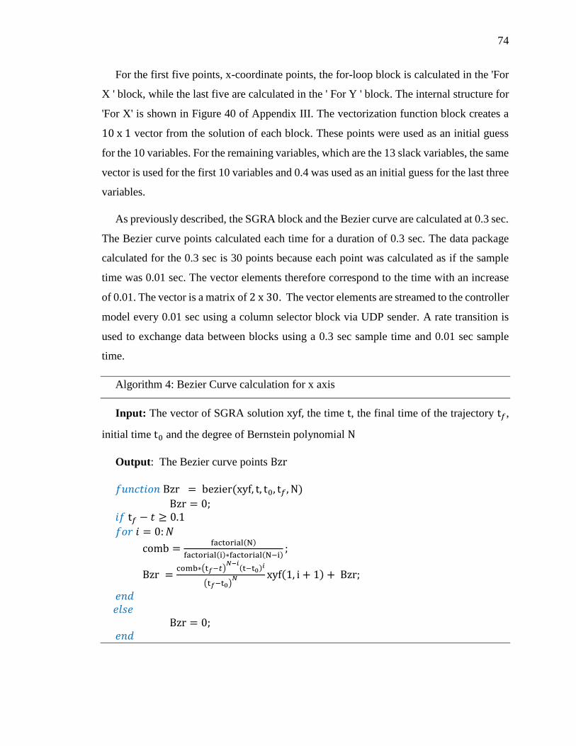
74

For the first five points, x-coordinate points, the for-loop block is calculated in the 'For

X ' block, while the last five are calculated in the ' For Y ' block. The internal structure for

'For X' is shown in Figure 40 of Appendix III. The vectorization function block creates a

10 x 1 vector from the solution of each block. These points were used as an initial guess

for the 10 variables. For the remaining variables, which are the 13 slack variables, the same

vector is used for the first 10 variables and 0.4 was used as an initial guess for the last three

variables.

As previously described, the SGRA block and the Bezier curve are calculated at 0.3 sec.

The Bezier curve points calculated each time for a duration of 0.3 sec. The data package

calculated for the 0.3 sec is 30 points because each point was calculated as if the sample

time was 0.01 sec. The vector elements therefore correspond to the time with an increase

of 0.01. The vector is a matrix of 2 x 30. The vector elements are streamed to the controller

model every 0.01 sec using a column selector block via UDP sender. A rate transition is

used to exchange data between blocks using a 0.3 sec sample time and 0.01 sec sample

time.

Algorithm 4: Bezier Curve calculation for x axis

Input: The vector of SGRA solution xyf, the time t, the final time of the trajectory t𝑓,

initial time t0 and the degree of Bernstein polynomial N

Output: The Bezier curve points Bzr

𝑓𝑢𝑛𝑐𝑡𝑖𝑜𝑛 Bzr = bezier(xyf, t, t0, t𝑓 , N)

Bzr = 0; 𝑖𝑓 t𝑓 − 𝑡 ≥ 0.1

𝑓𝑜𝑟 𝑖 = 0:𝑁

comb =factorial(N)

factorial(i)∗factorial(N−i);

Bzr =comb∗(t𝑓−𝑡)

𝑁−𝑖(t−t0)𝑖

(t𝑓−t0)𝑁 xyf(1, i + 1) + Bzr;

𝑒𝑛𝑑 𝑒𝑙𝑠𝑒 Bzr = 0; 𝑒𝑛𝑑

75

When the Bezier curve vector is calculated every 0.3 seconds, the initial time changes

each time. To describe it in detail, see Figure 34 below. At first the drone was at point 0.

During the first flight the drone moves from point 0 to 1 in 0.3 sec. This means that the

flight duration of 0.3 sec was already completed, therefore the initial time for the next flight

is the time at point 1. When the drone moves from point 1 to point 2, the same time, 0.3

sec, is used to cover the track. Then the next initial time becomes 0.6 sec or the time at

point 2. It will follow the same trends until the initial time is equal to the final time which

is the time the drones reached the destination.

Figure 34. The duration of time changes as the drone flies

As discussed earlier, the last two elements of the Bezier vector, 29th and 30th, are sent

to the extrapolation block to calculate the future points that will be used as the initial

position for the next calculation of the Bezier curve.

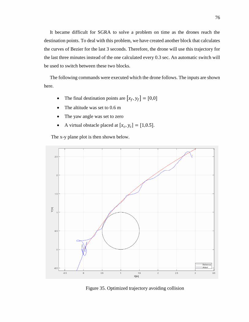
76

It became difficult for SGRA to solve a problem on time as the drones reach the

destination points. To deal with this problem, we have created another block that calculates

the curves of Bezier for the last 3 seconds. Therefore, the drone will use this trajectory for

the last three minutes instead of the one calculated every 0.3 sec. An automatic switch will

be used to switch between these two blocks.

The following commands were executed which the drone follows. The inputs are shown

here.

• The final destination points are [𝑥𝑓 , 𝑦𝑓] = [0,0]

• The altitude was set to 0.6 m

• The yaw angle was set to zero

• A virtual obstacle placed at [𝑥𝑐, 𝑦𝑐] = [1,0.5].

The x-y plane plot is then shown below.

Figure 35. Optimized trajectory avoiding collision

77

The x, y, and z plot separately is then shown in the following diagram.

Figure 36. The X, Y, Z and yaw angle plot

78

CHAPTER SEVEN

CONCLUSION

7.1. Summary

This thesis has presented the development of an indoor multirotor testbed lab and

guidance, navigation and control benchmark problems on multirotor. In chapter 3, a

detailed description of how to develop an experimental testbed laboratory for multirotor

was presented. Furthermore, I described how to control and fly an AR Drone using

Simulink as a ground controller and an OptiTrack MCS as system to retrieve position and

attitude information. In chapter 4, a strategy to execute an autonomous and accurate landing

was discussed. The obtained results show that this approach could be used for autonomous

battery charging purpose. In the same section I have also reported a methodology for

formation flight execution between two drones to reach an accurate steady alignment. In

chapter 5 a comparison between different nonlinear programming methods presented. The

performance of each solvers was compared based on the reliability and computational.

In chapter 6 one of the major sets back of battery powered drones was tackled through

the application of trajectory optimization. A trajectory was generated using a Bezier curve

by minimizing a jerk function. Minimization of jerk would have an indirect effect on the

power consumption.

7.2. Recommendation

The project included in this thesis paper, including accurate landing and optimization

of trajectories, is concerned with solving the energy consumption problem. In the precise

landing study, it was demonstrated that a drone can execute a precise landing on a mock-

up charging station. For this particular work, however, an actual battery charge was not

performed. With the landing accuracy achieved in this study, an actual autonomous battery

charging can be performed by building a charging station.

79

Another work included in this thesis paper was the use of trajectory optimization to

minimize energy consumption to solve the power problem with multirotor. In this area, we

have tried to reduce energy consumption by optimizing the trajectory minimizing the jerk.

How much this jerk reduction in trajectory generation would reduce energy consumption

should be studied for future work.

In addition, more work on optimizing SGRA and using it for real-time trajectory

optimization would solve the problem of finding an optimization solver that is fast enough

to solve an NLP so that it can be applied in real time.

80

REFERENCES

[1] Morbidi, F., Cano, R., and Lara, D., "Minimum-Energy Path Generation for a

Quadrotor UAV", IEE International Conference on Robotics and Automation,

Stockholm: 2016.

[2] Mahony, R., Kumar, V., and Corke, P., "Multirotor Aerial Vehicles: Modeling,

Estimation, and Control of Quadrotor", IEEE Robotics & Automation Magazine,

Vol. 19, No. 3, 2012, pp. 20-32.

[3] Theys, B., Dimitriadis, G., Hendrick, P., and Schutter, J. D., “Influence of propeller

configuration on propulsion system efficiency of multi-rotor Unmanned Aerial

Vehicles,” 2016 International Conference on Unmanned Aircraft Systems (ICUAS),

2016.

[4] Tsay, T., "Guidance and Control Laws for Quadrotor UAV", WSEAS

TRANSACTIONS on SYSTEMS and CONTROL, Vol. 9, 2014, pp. 606-613.

[5] Li, Q., “Grey-Box System Identification of a Quadrotor Unmanned Aerial Vehicle,”

thesis, 2014.

[6] YAOU, Z. H. A. N. G., WANSHENG, Z. H. A. O., TIANSHENG2 , L. U., and LI,

“The attitude control of the four-rotor unmanned helicopter based on feedback

linearization control,” WSEAS TRANSACTIONS on SYSTEMS, vol. 12, Apr. 2013.

[7] L’Afflitto, A., and Anderson, R., "Control AR Drone Parrot 2.0 with Matlab 2015a

and Vicon - File Exchange - MATLAB Central", Mathworks.com Available:

https://www.mathworks.com/matlabcentral/fileexchange/59177-control-ar-drone-

parrot-2-0-with-matlab-2015a-and-vicon.

[8] Cherfan, R., "MotiveExample - File Exchange - MATLAB

Central", Mathworks.comAvailable:

https://www.mathworks.com/matlabcentral/fileexchange/49085-motiveexample.

[9] Sanabria, D., "AR Drone Simulink Development-Kit V1.1 - File Exchange –

MATLAB Central", Mathworks.com Available:

https://www.mathworks.com/matlabcentral/fileexchange/43719-ar-drone-

simulink-development-kit-v1-1.

[10] Lee, D., "AR.Drone 2.0 Support from Embedded Coder - File Exchange –

MATLAB Central", Mathworks.com Available:

https://www.mathworks.com/matlabcentral/fileexchange/48558-ar-drone-2-0-

support-from-embedded-coder.

https://www.mathworks.com/matlabcentral/fileexchange/43719-ar-drone-simulink-development-kit-v1-1

https://www.mathworks.com/matlabcentral/fileexchange/43719-ar-drone-simulink-development-kit-v1-1

81

[11] Cichella, V., Kaminer, I., Xargay, E., Dobrokhodov, V., Hovakimyan, N., Aguiar,

A., and Pascoal, A., "A Lyapunov-based approach for Time-Coordinated 3D Path-

Following of Multiple Quadrotors", 51st IEEE Conference on Decision and

Control, Maui: 2012, pp. 1776-1781.

[12] “Developer Tools Downloads,” OptiTrackAvailable:

https://optitrack.com/downloads/developer-tools.html.

[13] "Calibration - NaturalPoint Product Documentation Ver

2.0", V20.wiki.optitrack.com Available:

https://v20.wiki.optitrack.com/index.php?title=Calibration.

[14] "Write Level-2 MATLAB S-Functions- MATLAB &

Simulink", Mathworks.comAvailable:

https://www.mathworks.com/help/simulink/sfg/writing-level-2-matlab-s-

functions.html#brgscav-1.

[15] Valenti, M., Dale, D., How, J., Farias, D. P. D., and Vian, J., “Mission Health

Management for 24/7 Persistent Surveillance Operations,” AIAA Guidance,

Navigation and Control Conference and Exhibit, 2007.

[16] Junaid, A. B., Lee, Y., and Kim, Y., “Design and implementation of autonomous

wireless charging station for rotary-wing UAVs,” Aerospace Science and

Technology, vol. 54, 2016, pp. 253–266.

[17] Junaid, A., Konoiko, A., Zweiri, Y., Sahinkaya, M., and Seneviratne, L.,

“Autonomous Wireless Self-Charging for Multi-Rotor Unmanned Aerial

Vehicles,” Energies, vol. 10, 2017, p. 803.

[18] Sani, M. F., and Karimian, G., “Automatic navigation and landing of an indoor AR.

drone quadrotor using ArUco marker and inertial sensors,” 2017 International

Conference on Computer and Drone Applications (IConDA), 2017.

[19] Carreira, T. G., “Quadcopter Automatic Landing on a Docking Station,” thesis,

2013.

[20] Levy, A. V., and Guerra, V., On the optimization of constrained functions:

comparison of sequential gradient-restoration algorithm and gradient projection

algorithm, Houston: Rice University, 1975.

[21] Box, M. J., “A Comparison of Several Current Optimization Methods, and the use

of Transformations in Constrained Problems,” The Computer Journal, vol. 9, Jan.

1966, pp. 67–77.

82

[22] Hock, W., and Schittkowski, K., “The Test Problems,” Lecture Notes in Economics

and Mathematical Systems Test Examples for Nonlinear Programming Codes,

1981, pp. 23–127.

[23] Svanberg, K., 2007.

[24] Mueller, M. W., Hehn, M., and Dandrea, R., “A computationally efficient algorithm

for state-to-state quadrocopter trajectory generation and feasibility

verification,” 2013 IEEE/RSJ International Conference on Intelligent Robots and

Systems, 2013.

[25] Michini, B., Toksoz, T., Redding, J., Michini, M., How, J., Vavrina, M., and Vian,

J., “Automated Battery Swap and Recharge to Enable Persistent UAV

Missions,” Infotech@Aerospace 2011, 2011.

[26] Ure, N. K., Chowdhary, G., Toksoz, T., How, J. P., Vavrina, M. A., and Vian, J.,

“An Automated Battery Management System to Enable Persistent Missions With

Multiple Aerial Vehicles,” IEEE/ASME Transactions on Mechatronics, vol. 20,

2015, pp. 275–286.

[27] Chang, T., and Yu, H., “Improving Electric Powered UAVs’ Endurance by

Incorporating Battery Dumping Concept,” Procedia Engineering, vol. 99, 2015, pp.

168–179.

[28] Gurdan, D., Stumpf, J., Achtelik, M., Doth, K.-M., Hirzinger, G., and Rus, D.,

“Energy-efficient Autonomous Four-rotor Flying Robot Controlled at 1

kHz,” Proceedings 2007 IEEE International Conference on Robotics and

Automation, 2007.

[29] Driessens, S., and Pounds, P., “The Triangular Quadrotor: A More Efficient

Quadrotor Configuration,” IEEE Transactions on Robotics, vol. 31, 2015, pp.

1517–1526.

[30] Yacef, F., Bouhali, O., and Hamerlain, M., “Optimization of Energy Consumption

for Quadrotor UAV,” International Micro Air Vehicle Conference and Flight

Competition, 2017, pp. 215–222.

[31] Fronza, I., Corral, L., Ioini, N. E., and Ibershimi, A., “Towards Optimization of

Energy Consumption of Drones with Software-Based Flight

Analysis,” Proceedings of the 28th International Conference on Software

Engineering and Knowledge Engineering, Jan. 2016.

83

[32] Cichella, V., Kaminer, I., Walton, C., and Hovakimyan, N., “Optimal Motion

Planning for Differentially Flat Systems Using Bernstein Approximation,” IEEE

Control Systems Letters, vol. 2, 2018, pp. 181–186.

[33] Eager, D., Pendrill, A.-M., and Reistad, N., “Beyond velocity and acceleration: jerk,

snap and higher derivatives,” European Journal of Physics, vol. 37, 2016, p.

065008.

[34] Smith, G., “Newton's Philosophiae Naturalis Principia Mathematica,” Stanford

Encyclopedia of PhilosophyAvailable: https://plato.stanford.edu/entries/newton-

principia/index.html#NewLawMot.

[35] Jeurgens, N., "Identification and Control Implementation of an AR.Drone 2.0",

Masters, Eindhoven University of Technology, 2017.

[36] Bangura, M., and Mahony, R., "Real-time Model Predictive Control for

Quadrotors", The International Federation of Automatic Control, Cape Town:

2014, pp. 11773-11780.

[37] Mahony, R., Kumar, V., and Corke, P., "Multirotor Aerial Vehicles: Modeling,

Estimation, and Control of Quadrotor", IEEE Robotics & Automation Magazine,

Vol. 19, No. 3, 2012, pp. 20-32.

[38] Mellinger, D., "Trajectory Generation and Control for Quadrotors", PhD, University

of Pennsylvania, 2012.

[39] "UAV Applications /// Drones for Inspection, Surveying & more", Ascending

Technologies Available: http://www.asctec.de/en/uav-uas-drone-applications/.

[40] Veeraklaew, T., Piromsopa, P., Chirungsarpsook, K., and Pattaravarangkur, C., “A

Study on the Comparison between Minimum Jerk and Minimum Energy of

Dynamic Systems,” International Conference on Computational Intelligence for

Modelling, Control and Automation and International Conference on Intelligent

Agents, Web Technologies and Internet Commerce (CIMCA-IAWTIC06).

84

APPENDIX I

NATNETSFUNCTION

1 function NatNetsFunction1(block) 2 % Level-2 MATLAB file S-Function for unit delay demo. 3 % Copyright 1990-2009 The MathWorks, Inc. 4 % $Revision: 1.1.6.3 $ 5 6 setup(block); 7 8 function setup(block) 9 10 block.NumDialogPrms = 1; 11 12 %% Register number of input and output ports 13 block.NumInputPorts = 2; 14 block.NumOutputPorts = 2; 15 %edited by Kidus for 2 outports 16 %% Setup functional port properties to dynamically 17 %% inherited. 18 %block.SetPreCompInpPortInfoToInherited; 19 %block.SetPreCompOutPortInfoToInherited; 20 21 block.InputPort(1).Dimensions = 1; 22 block.InputPort(2).Dimensions = 1; 23 %added by Kidus for two ports 24 block.InputPort(1).DirectFeedthrough = false; 25 26 block.OutputPort(1).Dimensions = 6; 27 block.OutputPort(2).Dimensions = 6; 28 29 %% Set block sample time to [0.01 0] 30 block.SampleTimes = [0.01 0]; 31 %%%%%%%%%%%%%%%%%%%%%%%%%% Changed from 0.01 to 0.02

%%%%%%%%%%%%%%% 32 33 %%Set the block simStateCompliance to default(i.e.,same as a

built-in block) 34 block.SimStateCompliance = 'DefaultSimState'; 35 36 %% Register methods 37 block.RegBlockMethod('PostPropagationSetup',

@DoPostPropSetup); 38 block.RegBlockMethod('InitializeConditions',

@InitConditions); 39 block.RegBlockMethod('Outputs', @Output); 40 block.RegBlockMethod('Update', @Update); 41 block.RegBlockMethod('Terminate', @Terminate); 42 43 %added by Kidus 44block.RegBlockMethod('SetInputPortSamplingMode',@SetInputPortSampli

ngMode); 45 % block.RegBlockMethod('SetInputPortDimensions',

@SetInpPortDims); 46 % block.RegBlockMethod('Outputs', @Output);

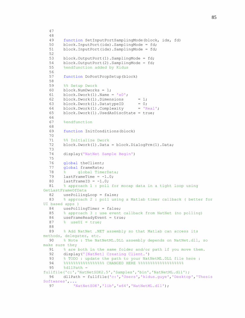
85

47 48 49 function SetInputPortSamplingMode(block, idx, fd) 50 block.InputPort(idx).SamplingMode = fd; 51 block.InputPort(idx).SamplingMode = fd; 52 53 block.OutputPort(1).SamplingMode = fd; 54 block.OutputPort(2).SamplingMode = fd; 55 %endfunction added by Kidus 56 57 function DoPostPropSetup(block) 58 59 %% Setup Dwork 60 block.NumDworks = 1; 61 block.Dwork(1).Name = 'x0'; 62 block.Dwork(1).Dimensions = 1; 63 block.Dwork(1).DatatypeID = 0; 64 block.Dwork(1).Complexity = 'Real'; 65 block.Dwork(1).UsedAsDiscState = true; 66 67 %endfunction 68 69 function InitConditions(block) 70 71 %% Initialize Dwork 72 block.Dwork(1).Data = block.DialogPrm(1).Data; 73 74 display('NatNet Sample Begin') 75 76 global theClient; 77 global frameRate; 78 % global TimerData; 79 lastFrameTime = -1.0; 80 lastFrameID = -1.0; 81 % approach 1 : poll for mocap data in a tight loop using

GetLastFrameOfData 82 usePollingLoop = false; 83 % approach 2 : poll using a Matlab timer callback ( better for

UI based apps ) 84 usePollingTimer = false; 85 % approach 3 : use event callback from NatNet (no polling) 86 useFrameReadyEvent = true; 87 % useUI = true; 88 89 % Add NatNet .NET assembly so that Matlab can access its

methods, delegates, etc. 90 % Note : The NatNetML.DLL assembly depends on NatNet.dll, so

make sure they 91 % are both in the same folder and/or path if you move them. 92 display('[NatNet] Creating Client.') 93 % TODO : update the path to your NatNetML.DLL file here : 94 %%%%%%%%%%%%%%%%% CHANGED HERE %%%%%%%%%%%%%%%%%%% 95 %dllPath =

fullfile('c:','NatNetSDK2.5','Samples','bin','NatNetML.dll'); 96 dllPath = fullfile('c:','Users','kidus.guye','Desktop','Thesis

Softwares',... 97 'NatNetSDK','lib','x64','NatNetML.dll');

86

98 assemblyInfo = NET.addAssembly(dllPath); 99 100 % Create an instance of a NatNet client 101 theClient = NatNetML.NatNetClientML(0); % Input =

iConnectionType: 0 = Multicast, 1 = Unicast 102 version = theClient.NatNetVersion(); 103 fprintf( '[NatNet] Client Version : %d.%d.%d.%d\n',

version(1),... 104 version(2), version(3), version(4) ); 105 106 % Connect to an OptiTrack server (e.g. Motive) 107 display('[NatNet] Connecting to OptiTrack Server.') 108 hst = java.net.InetAddress.getLocalHost; 109 110 111 %%%%%%%%%%%%%%%%% CHANGED HERE %%%%%%%%%%%%%%%%%%% 112 %HostIP = char(hst.getHostAddress); 113 HostIP = char('127.0.0.1');%Get IP 114 flg = theClient.Initialize(HostIP, HostIP); % Flg = returnCode:

0 = Success 115 if (flg == 0) 116 display('[NatNet] Initialization Succeeded') 117 else 118 display('[NatNet] Initialization Failed') 119 end 120 121 % print out a list of the active tracking Models in Motive 122 GetDataDescriptions(theClient) 123 124 % Test - send command/request to Motive 125 [byteArray, retCode] =

theClient.SendMessageAndWait('FrameRate'); 126 if(retCode ==0) 127 byteArray = uint8(byteArray); 128 frameRate = typecast(byteArray,'single'); 129 end 130 global theClient; 131 global data; 132 data = theClient.GetLastFrameOfData(); 133 134 function Output(block) 135 136 %block.OutputPort(1).Data = block.Dwork(1).Data; 137 % global theClient; 138 global data; 139 % java.lang.Thread.sleep(0.1); 140 % data = theClient.GetLastFrameOfData(); 141 D=ProcessFrame(data); 142

block.OutputPort(1).Data=double([D.x;D.y;D.z;D.angleX;D.angleY;D.angleZ

]); 143 block.OutputPort(2).Data =

double([D.x1;D.y1;D.z1;D.angleX1;D.angleY1;... 144 D.angleZ1]); 145 %edited by Kidus Guye to check for two rigid 146 % bodies at the same time 147

87

148 149 150 function Update(block) 151 global theClient; 152 global data; 153 block.Dwork(1).Data = block.InputPort(1).Data; 154 data = theClient.GetLastFrameOfData(); 155 156 %endfunction 157 158 function Terminate(block) 159 global theClient; 160 % global TimerData; 161 theClient.Uninitialize(); 162 % % Sheng's test on polling data CLEAN UP!! 163 % stop(TimerData); 164 % delete(TimerData); 165 % % eng Sheng's clean up 166 167 disp('NatNet Sample End') 168 169 170 %endfunction 171 172 function [D] = ProcessFrame( frameOfData ) 173 174 rigidBodyData = frameOfData.RigidBodies(1); 175 rigidBodyData1 = frameOfData.RigidBodies(2); 176 % Position 177 178 D.x = rigidBodyData.z; 179 D.y = -rigidBodyData.x; 180 D.z = -(rigidBodyData.y); 181 %second rigid body 182 D.x1 = rigidBodyData1.z; 183 D.y1 = -rigidBodyData1.x; 184 D.z1= -(rigidBodyData1.y); 185 %edited Kidus for two rigid 186 187 q = quaternion( rigidBodyData.qx, rigidBodyData.qy,

rigidBodyData.qz,... 188 rigidBodyData.qw ); 189 190 qRot = quaternion( 0, 0, 0, 1);% rotate pitch 180 to avoid

180/-180 flip for nicer graphing 191 q = mtimes(q, qRot); 192 % 193 %%edited by Kidus to get the yaw, pitch and roll angles 194 angles = EulerAngles(q,'zyx'); 195 D.angleX = -angles(1)* 180.0 / pi; % must invert due to 180

flip above 196 D.angleY = angles(2)*180.0 / pi; 197 D.angleZ = -angles(3)*180.0 / pi; % must invert due to 180

flip above 198 %added by Kidus 199 q1 =

quaternion(rigidBodyData1.qx,rigidBodyData1.qy,rigidBodyData1.qz,...

88

200 rigidBodyData1.qw ); 201 202 qRot1 = quaternion( 0, 0, 0, 1); % rotate pitch 180 to avoid

180/-180 flip for nicer graphing 203 q1 = mtimes(q1, qRot1); 204 % 205 %edited by Kidus to get the yaw, pitch and roll angles 206 angles1 = EulerAngles(q1,'zyx'); 207 D.angleX1 = -angles1(1)* 180.0 / pi; % must invert due to 180

flip above 208 D.angleY1 = angles1(2)*180.0 / pi; 209 D.angleZ1 = -angles1(3)*180.0 / pi; 210 %Edited by Kidus for the second RGB 211 212 function GetDataDescriptions( theClient ) 213 214 dataDescriptions = theClient.GetDataDescriptions(); 215 216 % print out 217 fprintf('[NatNet] Tracking Models : %d\n\n',

dataDescriptions.Count); 218 for idx = 1 : dataDescriptions.Count 219 descriptor = dataDescriptions.Item(idx-1); 220 if(descriptor.type == 0) 221 fprintf('\tMarkerSet \t: '); 222 elseif(descriptor.type == 1) 223 fprintf('\tRigid Body \t: '); 224 elseif(descriptor.type == 2) 225 fprintf('\tSkeleton \t: '); 226 else 227 fprintf('\tUnknown data type : '); 228 end 229 fprintf('%s\n', char(descriptor.Name)); 230 end 231 232 for idx = 1 : dataDescriptions.Count 233 descriptor = dataDescriptions.Item(idx-1); 234 if(descriptor.type == 0) 235 fprintf('\n\tMarkerset : %s\t(%d markers)\n',

char(descriptor.Name),... 236 descriptor.nMarkers); 237 markerNames = descriptor.MarkerNames; 238 for markerIndex = 1 : descriptor.nMarkers 239 name = markerNames(markerIndex); 240 fprintf('\t\tMarker : %-20s\t(ID=%d)\n',

char(name),markerIndex); 241 end 242 elseif(descriptor.type == 1) 243 fprintf('\n\tRigid Body : %s\t\t(ID=%d, ParentID=%d)\n',... 244 char(descriptor.Name),descriptor.ID,descriptor.parentID); 245 elseif(descriptor.type == 2) 246 fprintf('\n\tSkeleton : %s\t(%d bones)\n',

char(descriptor.Name),... 247 descriptor.nRigidBodies); 248 %fprintf('\t\tID : %d\n', descriptor.ID); 249 rigidBodies = descriptor.RigidBodies; 250 for boneIndex = 1 : descriptor.nRigidBodies

89

251 rigidBody = rigidBodies(boneIndex); 252 fprintf('\t\tBone : %-20s\t(ID=%d, ParentID=%d)\n',

char(rigidBody.Name),... 253 rigidBody.ID, rigidBody.parentID); 254 end 255 end 256 end 257 %endfunction

APPENDIX II

INITIAL VARIABLES

1 sampleTime = 0.01;

2

3 kz = 1;

4 kzi = 0;

5 %pitch/forward velocity controller gains

6 Kpt = 0.4;%pid proportional gain

7 Kit = 0;%pid integral gain

8 Kdt =0.45;%pid derivative gain

9 Kanglet = 0.3;

10 %roll/lateral velocity controller gains

11 Kpf = 0.45;%pid proportional gain

12 Kif = 0;%pid integral gain

13 Kdf =0.45;%pid derivative gain

14 Kanglef = -0.2;

15

16 %yaw rate controller gains

17 kpsi = 1.9;

18 kpsil =0.075;

90

APPENDIX III

Figure 37. x and y position capture at t = ts

Figure 38. The second initial point extrapolation block

91

Figure 39. Initial guess starter block

Figure 40. For loop to calculate the initial guess

92

Figure 41. SGRA block content

Figure 42. Bezier Curve block

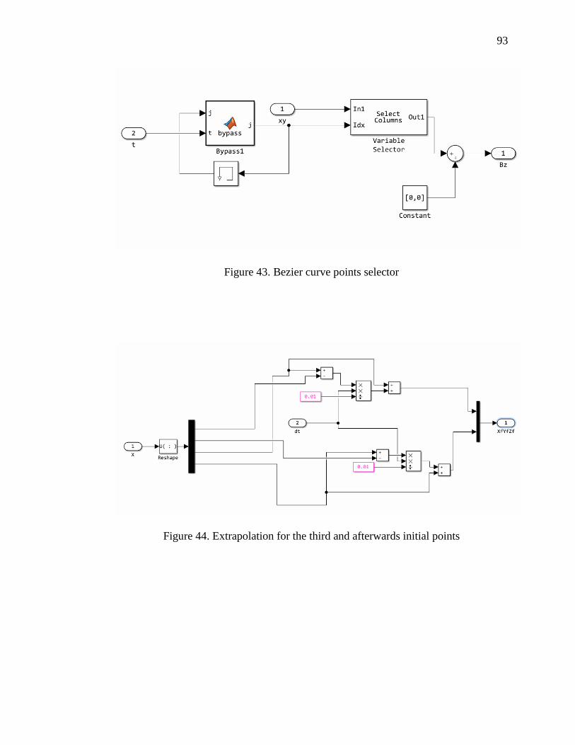
93

Figure 43. Bezier curve points selector

Figure 44. Extrapolation for the third and afterwards initial points

Development of an Indoor Multirotor Testbed for ...

Documents

Transcript of Development of an Indoor Multirotor Testbed for ...