DEVELOPMENT OF A THULIUM GERMANATE THIN DISK LASER ...
101
DEVELOPMENT OF A THULIUM GERMANATE THIN DISK LASER PROTOTYPE by Daniel Sickinger A Thesis Submitted to the Faculty of the COLLEGE OF OPTICAL SCIENCES In Partial Fulfillment of the Requirements For the Degree of MASTER OF SCIENCE In the Graduate College THE UNIVERSITY OF ARIZONA 2016
Transcript of DEVELOPMENT OF A THULIUM GERMANATE THIN DISK LASER ...
DEVELOPMENT OF A THULIUM GERMANATE
THIN DISK LASER PROTOTYPE
by
Daniel Sickinger
A Thesis Submitted to the Faculty of the
COLLEGE OF OPTICAL SCIENCES
In Partial Fulfillment of the Requirements
For the Degree of
MASTER OF SCIENCE
In the Graduate College
THE UNIVERSITY OF ARIZONA
2016
STATEMENT BY AUTHOR
The thesis titled Development of a Thulium Germanate Thin Disk
Laser Prototype prepared by Daniel Sickinger has been submitted in partial
fulfillment of requirements for a master’s degree at the University of Arizona and
is deposited in the University Library to be made available to borrowers under
rules of the Library.
Brief quotations from this thesis are allowable without special permission,
provided that an accurate acknowledgement of the source is made. Requests for
permission for extended quotation from or reproduction of this manuscript in
whole or in part may be granted by the head of the major department or the Dean
of the Graduate College when in his or her judgment the proposed use of the
material is in the interests of scholarship. In all other instances, however,
permission must be obtained from the author.
SIGNED: Daniel Sickinger
APPROVAL BY THESIS DIRECTOR
This thesis has been approved on the date shown below:
Defense Date
Xiushan Zhu 5/9/2016
Associate Research Professor
of Optical Sciences
i
Abstract
A Thulium Germanate thin disk laser prototype is developed and its potential
applications are discussed. Unfortunately, the thin disk gain material for the CW
prototype was unable to lase due to thermal limitations within the disk. However,
a CW output power model and a physical pump chamber module have been
developed, along with the supporting Zemax models and alignment procedures so
other gain materials and future improvements can be tested.
[1] [2] [3] [4] [5] [6] [7] [8] [9] [10] [11] [12] [13] [14] [15] [16] [17] [18] [19]
[20] [21] [22] [23] [24] [25] [26]
ii
Acknowledgements
I would like to take the time to first thank those who have helped me develop
and understand lasers fundamentally, most notably, my advisor Xiushan Zhu and
Valery Temyanko. Their ability to patiently answer my questions was invaluable
to the experience I developed throughout this project.
People to also thank are, Rolland Himmelhuber and Sasaan Showghi for
opinions and ideas to point me in the right directions, as well as Todd Horne for
the use of the machine shop and tools.
Finally and most importantly, I would like to thank my parents, who I love
dearly, for always being there for me under any experience I was facing in life.

iii
Contents
Abstract ................................................................................................................... i
Acknowledgements ............................................................................................... ii
Contents ................................................................................................................ iii
List of Figures ....................................................................................................... vi
List of Tables ...................................................................................................... viii
1. Introduction ...................................................................................................... 1
1.1 History ...................................................................................................... 2
Rectangular Thin Slab Laser ................................................................... 2
Zig-Zag Thin Slab Laser .......................................................................... 3
Thin Disk Laser ........................................................................................ 4
1.2 Areas of Interest ....................................................................................... 7
Military Applications ............................................................................... 7
Medical Applications ............................................................................... 8
Material Processing ................................................................................. 8
Laser Sensing and Spectroscopy .............................................................. 9
1.3 Thulium Germanate Thin Disk as Potential ............................................. 9
Thulium Germanate as Gain Medium .................................................... 10
Thulium Germanate as a Thin Disk Laser ............................................. 11
1.4 Motivation and Intent ............................................................................. 12
2. Thin Disk Laser Basics .................................................................................. 13
2.1 Laser Gain Medium ................................................................................ 15
Amplifying Atoms ................................................................................... 15
Host Material ......................................................................................... 17
2.2 Laser Oscillator ...................................................................................... 18
iv
Cavity Configurations ............................................................................ 18
Resonator Types ..................................................................................... 19
2.3 Pumping Configuration .......................................................................... 21
Pump Chamber ...................................................................................... 22
Source Optics ......................................................................................... 24
3. Laser Fundamentals and Modelling ............................................................ 25
3.1 Light Interactions ................................................................................... 25
Spontaneous Emission............................................................................ 27
Absorption .............................................................................................. 27
Stimulated Emission ............................................................................... 28
3.2 Laser Operation ...................................................................................... 28
Three Level System................................................................................. 29
Laser Assumptions ................................................................................. 31
3.3 Rate Equations........................................................................................ 33
Population Rate Equations .................................................................... 33
Photon Rate Equations........................................................................... 34
3.4 Gain Threshold ....................................................................................... 35
3.5 Pump Chamber Power Contribution ...................................................... 36
3.6 Resonator Effects ................................................................................... 39
Signal Aperture Effect ............................................................................ 39
Pump-Signal Coupling Value................................................................. 40
3.7 CW Power Output Model ....................................................................... 41
Output Power Equations ........................................................................ 41
Yb:YAG Thin Disk Laser Comparison ................................................... 42
4. Thin Disk Prototype Design .......................................................................... 45
4.1 Design Summary .................................................................................... 46
First Order Summary ............................................................................. 46
4.2 Component Selection and Manufacture ................................................. 47
Pump Source .......................................................................................... 47
Collimation Optics ................................................................................. 47
v
Parabolic Mirror.................................................................................... 48
Fold Mirrors .......................................................................................... 48
Thin Disk ................................................................................................ 49
Thin Disk Heatsink ................................................................................. 50
Resonator Configuration........................................................................ 51
Final System Layout ............................................................................... 52
4.3 Alignment and Assembly ....................................................................... 55
Thin Disk Reference Mirror to Parabolic Mirror .................................. 56
Four Fold Mirrors ................................................................................. 58
Pump Source and Collimation Optics .................................................... 60
Thin Disk and Resonator Optics ............................................................ 62
5. System Performance ...................................................................................... 63
5.1 Pump Spot Analysis ............................................................................... 63
Fiber Source ........................................................................................... 64
Pump Spot .............................................................................................. 65
Tm:Germanate Output Power Model .................................................... 67
Experimental Results and Conclusion ................................................... 69
Appendix A – MATLAB Model Code for Tm:Germanate ............................. 72
Appendix B – ZEMAX Pump Design Procedure ............................................. 75
Appendix C - Pump Chamber Alignment Procedure ..................................... 79
Appendix D – Mechanical Drawings ................................................................. 84
Parabolic Mirror ............................................................................................. 84
Parabolic Mirror Mounting Bracket .............................................................. 85
Thin Disk Heatsink ........................................................................................ 86
Thin Disk Water Adapter ............................................................................... 87
References ............................................................................................................ 88
vi
List of Figures
1.1 Rectangular thin slab concept [5]………………………………………….. 2
1.2 Zig-Zag thin slab laser concept [5]………………………………………… 3
1.3 Schematic view of the thin disk laser design [15]…………………………. 4
1.4 Power output from a single disk Trumpf Yb:YAG thin disk laser [15]...... 5
1.5 Schematic view of the thin disk laser pumping scheme [8]……………….. 6
1.6 Thin Disk Module TDM 1.0 SMA courtesy of Dausinger+Guisen GMBH. 6
1.7 Absorption of water [17]…………………………………………………... 7
1.8 Thulium energy level scheme……………………………………………… 10
1.9 Thulium Germanate cross-section absorption and emission curves [12]….. 10
2.1 Essential laser components………………………………………………… 13
2.2 Elements of a Thin Disk Laser…………………………………………….. 14
2.3 Doping atoms in a host material…………………………………………… 15
2.4 Wavelength emissions for various gain materials [5]……………………... 16
2.5 Thin disk laser various cavity configurations……………………………… 18
2.6 Example of thin disk module stacking for high output power…………….. 19
2.7 Common stable resonator configurations [5]……………………………… 20
2.8 Thin disk pump scheme using Non-Sequential Zemax……………………. 21
2.9 Two-dimensional thin disk pump concept…………………………………. 22
2.10 Thin disk’s four fold mirrors beam directions……………………………... 23
2.11 Source optics into pump chamber…………………………………………. 24
3.1 Absorption and emission interactions……………………………………... 26
3.2 Three level diagram of Thulium…………………………………………… 29
3.3 Simplified energy level diagram of Thulium……………………………… 32
3.4 Gain and absorption of the gain material………………………………….. 34
3.5 Linear cavity signal ray propagation for gain threshold…………………... 35
3.6 Pump light losses as beam folds around pump chamber………………….. 37
3.7 Aperture effect of pump focus in thin disk laser…………………………... 40
3.8 Power Output vs Power Input for theoretical and measured data of the
Yb:YAG laser……………………………………………………………… 43
4.1 Pump source in designed system…………………………………………... 47
4.2 Collimation optics in designed system…………………..………………… 47
4.3 Parabolic mirror……………………………………………………………. 48
4.4 Fold mirrors in designed system…………………………………………… 48
4.5 Interferometer measurements using a WYKO 6000………………………. 49
4.6 Tm:Germanate thin disk in designed system………………………………. 49
4.7 Thin disk heatsink copper piece…………………………………………… 50
4.8 Thin disk heatsink water cooling process………………………………….. 50

vii
4.9 Thin disk heatsink and cooling apparatus…………………………………. 50
4.10 Tm:Germanate resonator configuration…………………………………… 51
4.11 Solidworks model of pump module……………………………………….. 52
4.12 Solidworks model of pump optics…………………………………………. 52
4.13 Non-Sequential Zemax Layout (view 1 and 2)……………………………. 53
4.14 Non-Sequential Zemax Layout of 20 beams………………………………. 53
4.15 Real System layout………………………………………………………… 54
4.16 Pump optics layout (zoomed in)…………………………………………… 54
4.17 Pump chamber alignment using an interferometer as a large diameter
collimator…………………………………………………………………... 55
4.18 Parabolic mirror and thin disk alignment concept…………………………. 56
4.19 Pinhole misalignment characteristics for parabola to thin disk alignment... 57
4.20 Thin disks four fold mirrors alignment concept…………………………… 58
4.21 Angle adjustment of four fold mirrors…………………………………….. 59
4.22 Source optics alignment concept………………………………………….. 60
4.23 Prototype of source optics and pump chamber…………………………….. 61
4.24 Source optics beam alignment characteristics……………………………... 61
4.25 Resonator alignment concept………………………………………………. 62
5.1 Zemax modelled data from a DILAS 793nm fiber diode………………….. 64
5.2 Pump spot’s cross section at the thin disk focus…………………………... 65
5.3 Pump spot on thin disk HR side (zoomed in)……………………………… 66
5.4 Comparison of pump spot on thin disk HR side…………………………… 66
5.5 Tm:Germanate power output vs power input for various s-p coupling
values………………………………………………………………………. 68
5.6 Pump spot temperature experience in thin disk……………………………. 69
5.7 Tm:Germanate thin disk temperature vs power input for various
interface materials….…………………………………………….……….... 70
5.8 Pump spot temperature in Yb:YAG thin disk laser………………………... 71

viii
List of Tables
2.1 Effects of different host materials using Thulium [2]……………………... 17
3.1 Dausinger-Guisen Yb:YAG system parameters for modelling……………. 42
3.2 Comparison of the slope efficiency and signal pump coupling values……. 44
3.3 Model Verification using Threshold Difference…………………………... 44
4.1 Summary of first order Tm:Germanate design…………………………….. 46
5.1 Tm:Germanate Model Parameters…………………………………………. 67
5.2 Threshold and slope efficiency values for various s-p coupling values…… 68

1
Chapter 1
Introduction
For several decades, laser designs have greatly evolved to accommodate the
demand for higher power, smaller size, better efficiency, and lower input power
requirements. In the past 17 years, thin disk lasers have been of particular interest
due to its ability to meet these increasing demands while allowing moderate costs
for manufacture, power scalability, and good output beam quality [1].
Furthermore, thin disk lasers have the ability be scaled to large powers and to
use a wide range of gain materials for various wavelength output emissions. In
particular, the 2μm region is of interest due to laser sensing/spectroscopy, medical
applications, material processing, free space optical communications, and military
applications [2].
This thesis presents the design and manufacture of a prototype CW thin disk
laser using Thulium-Germanate as a prototype for further research and
development. Future experiments using different active gain media and enhanced
laser techniques such as Q-switching and Mode-Locking can be used with the
manufactured design.

2
1.1 History
The LASER, which is an acronym for Light Amplification by Stimulated
Emission of Radiation, was first demonstrated by Theodore Maiman in 1960
using Ruby. Since then, lasers have gone through revolutionary changes and have
developed into countless design configurations using different kinds of atoms,
molecules, and ions, in the form of gasses, liquids, crystals, glasses, plastics, and
semiconductors [4]. Of the various designs invented, each has suffered its own
set of limitations such as inadequate power, damage in the gain medium, poor
beam quality, and erratic mode behavior. To combat such issues and improve
solid-state laser capabilities, initial designs went through multiple iterations using
unique configurations. Nevertheless, all designs encompass the same basic
physics of stimulated and spontaneous emission first theorized by Einstein in
1917.
Rectangular Thin Slab Laser
Figure 1.1 Rectangular thin slab concept [5].
3
Before the thin disk laser, one of the first improvements started as a thin slab
laser utilizing both sides of the gain medium pumped with light. This design
improved on existing bulk rod designs by giving a larger cooling surface and
twice the pump power. In return, this gave the system more laser power and a
one-dimensional temperature gradient across the thickness of the slab [5].
Unfortunately, this design had low performance once pump powers were
increased since the slab would experience large thermal lensing and eventually
fracture. This lead to catastrophic failure and limited the scalability of the design.
Zig-Zag Thin Slab Laser
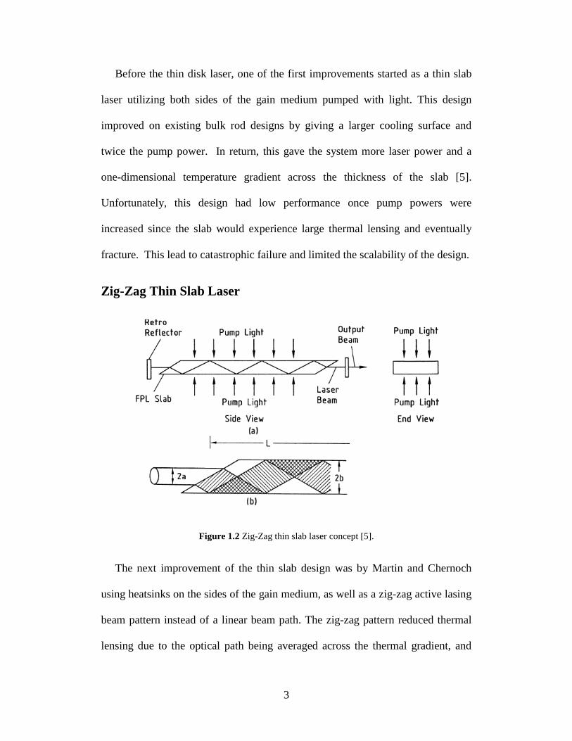
Figure 1.2 Zig-Zag thin slab laser concept [5].
The next improvement of the thin slab design was by Martin and Chernoch
using heatsinks on the sides of the gain medium, as well as a zig-zag active lasing
beam pattern instead of a linear beam path. The zig-zag pattern reduced thermal
lensing due to the optical path being averaged across the thermal gradient, and

4
also minimized stress induced birefringence due to the rectilinear cross section
[9]. However, the design was limited by residual distortions at the slab ends and
pump faces, as well as mechanical mounting complications, low efficiency, and
high fabrication costs [5]. Also, the thickness and cooling efficiency was greatly
decoupled causing large variations in one parameter when the other was slightly
modified.
Thin Disk Laser
To further improve thin slab lasers, researchers at the University of Stuttgart in
1994 published a new way to mount a round thin slab (thin disk) to a heatsink and
pump the disk axially.
Figure 1.3 Schematic view of the thin disk laser design [15].

5
In this design configuration, the active gain medium has a thickness ranging
from 100μm to 500μm with a disk diameter ranging from 5mm to 10mm [23].
The surface mounted to the thin disk is coated with a highly reflective coating and
serves as one of the resonator mirrors. Heat in the thin disk is extracted one-
dimensionally along the optical axis directly to the heatsink, which efficiently
removes the heat generated from the pump source and active lasing region. This
ultimately minimizes stresses, radial thermal gradients, and refraction index
variations, especially when the thickness is relatively small compare to the thin
disk’s diameter [5]. This novel concept allows the laser to obtain kilowatts of
average power at room temperature while maintaining good beam quality, ideal
pulse characteristics, and high efficiency [15].
Figure 1.4 Power output from a single disk Trumpf Yb:YAG thin disk laser [15].

6
To achieve such high output powers, multiple passes through the thin disk are
required. This is done by using a single source laser and creatively coupling it
with several optical elements to fold the beam multiple times over the same spot.
This allows the gain medium to experience high source powers typically ranging
from 6 to 20 times the initial source power.
Figure 1.5 Schematic view of the thin disk laser pumping scheme [8].
The thin disk laser module can also be a very compact system for the power
output. As can be seen below in figure 1.6, the Dausinger-Guisen module has
dimensions of 311mm x 122mm and uses the supporting housing to efficiently
cool the system. Using the same pump power density, the system can host a wide
range pump powers up to 250W by simply scaling up the spot size.
Figure 1.6. Thin Disk Module TDM 1.0 SMA courtesy of Dausinger+Guisen GMBH.

7
1.2 Areas of Interest
The regions of 450nm to 550nm and 1860nm to 1945nm are of interest due to
its low and high absorption peaks in water. Other materials are also of interest
due to their high absorption peaks near 2μm. This provides the ability to advance
new technologies not available in the past from lack of power and capability.
Figure 1.7 Absorption of water [17].
Military Applications
Eye Safe Targeting Devices - Many incidents have been reported from
battlefield conditions and unsafe use where users are blinded by a friendly
laser sweeping across a combat zone [16]. Water in the vitreous portion of
the eye heavily absorbs the 2um wavelength region and prevents
damaging radiation from injuring the retina. This is particularly ideal for
8
small unit laser systems such as designators and IR targeting systems,
where the lasers can be pointed at other friendly soldier’s faces.
LIDAR and Scanning Systems - Multilevel harmonic generation can be
used to obtain a wavelength near 475nm. In this wavelength region, light
is least absorbed by water. This creates the potential for mapping
underwater regions for detection of submarines, mines, combatants, and
other debris [2].
Medical Applications
High Absorption and Low Penetration Depth – Once again, as an
application due to high absorption in water, the 2μm laser provides the
ability for high precision surgical processes for both soft and hard tissues
[2]. Compared to other laser wavelengths, 2μm laser radiation helps to
suppress bleeding during surgical operations and limits heat induced
damage in the surrounding tissue.
Material Processing
Plastic Cutting, Welding, and Marking – Since existing wieldable plastics
are highly transparent near the 1μm region, they need very high CW
powers and must be mixed with additional compounds to make the plastic
wieldable [2]. Wavelengths around 2μm are highly absorbed in many
plastics. This provides the ability to weld existing plastics with high
quality joints and limit the amount of toxic substances released during the
welding process.
9
Laser Sensing and Spectroscopy
Element and Atmospheric Detection – A number of atmospheric gases
such as water, carbon dioxide, and nitrogen oxide all have absorption lines
near the 2um region. Using CW and pulsed systems, these gases can be
used to detect and analyze atmospheric conditions [2].
1.3 Thulium Germanate Thin Disk as Potential
Since the thin disk architecture has only been discovered in the past 17 years,
new materials have not been extensively investigated yet. Other host materials
such as Tm:YAG, Tm:YLF, and Tm:YAP have been used, but they have shown
limitations such as birefringence, low damage threshold, or high manufacturing
costs.
One such material to meet increasing requirements is Thulium Germanate;
unfortunately it is a fairly new material and there is no information about its use
as a thin disk laser. Comparatively, Tm3+
doped crystals in fiber platforms have
shown great benefits such as its high efficiency and long radiative lifetimes [2].
Germanate glass has also shown great benefits as a host matrix due to its
combination of good thermal stability, high solubility, low phonon energy, lack of
birefringent dependence, and high transparency in a wide wavelength range [10].

10
Thulium Germanate as Gain Medium
Figure 1.8 Thulium energy level scheme.
Pump radiation at 793nm transfers Tm3+
ions from the 3H6 ground state into
the 3H4 pump state. At this point, the excitation undergoes a transition from
3H4 to
3F4, while an unexcited ion undergoes a transition from
3H6 to
3F4 due to a self-
relaxation process. Ultimately, this process creates two ions in the upper state for
every one photon absorbed, giving a quantum efficiency of 2.
Figure 1.9 Thulium Germanate cross-section absorption and emission curves [12].
11
According to measured data from NP Photonics, Thulium Germanate has an
ideal emission wavelength region of 1600 to 2000nm, and also has a high
absorption peak wavelength of 793nm. The emission spectrum meets the
requirements for many applications, and the absorption wavelength is ideal since
Thulium Germanate can be pumped by an easily obtainable commercial fiber
laser module at 793nm. Also, germanate glass as a host has shown lower phonon
energy (900 cm-1)
compared to silica glass (1100 cm-1
) which helps to increase the
quantum efficiency and reduce the non-radiative decay rate of the upper lasing
level of 3F4 [24]. Germanate can also be doped much higher due to its higher
solubility of Thulium from a lower quenching effect [25].
Thulium Germanate as a Thin Disk Laser
Quasi-three-level materials have shown the highest efficiency in thin disk
lasers, but can be difficult to operate because the laser wavelength experiences
high absorption from the ground state being so close to the lower laser level [7].
This requires high pump intensities and low temperatures in the crystal to achieve
laser threshold. Thulium Germanate, a quasi-three-level material, gives the
opportunity to achieve such high efficiencies, but risks experiencing high
temperatures inside the material. Using Thulium Germanate in a thin disc system
can obtain very high powers by utilizing the heat sink and by scaling the pump
diameter similar to other Yb:YAG thin disk lasers. It can also be used as a high
energy system due to the short gain medium making it ideal for Q-switching and
mode-locking. This is of high interest and would provide a great improvement
over currently limited fiber systems.
12
1.4 Motivation and Intent
The desire to design and manufacture a working prototype of a Thulium
Germanate thin disk laser is of high importance. Such a device can open up new
research opportunities and create the ability to enhance areas in laser sensing and
spectroscopy, medical applications, material processing, and military applications.
The prototype system will have a broadband high reflection coating centered
around 795nm on the pump chamber optics. This coating region allows for
investigations into other host materials whose absorption wavelength falls around
this value. Having the capability to investigate different host materials gives the
option to develop new technologies and expand further research.
Also, the prototype was designed to be a cheap experimentation version to
study of the characteristics within the thin disk architecture. The prototype is not
meant as a final product and is intended to learn many aspects of the design.
Having a starting prototype allows for cost efficient investigations into heating
effects, pumping characteristics, lasing parameters, and issues not yet
encountered. Learning these parameters enhances future iterations so a newer
system can be more robust, obtain higher powers, have better efficiency, as well
as provide the opportunity to experiment with Q-switching and mode-locking
techniques. Without a CW prototype to investigate, none of this is possible.
13
Chapter 2
Thin Disk Laser Basics
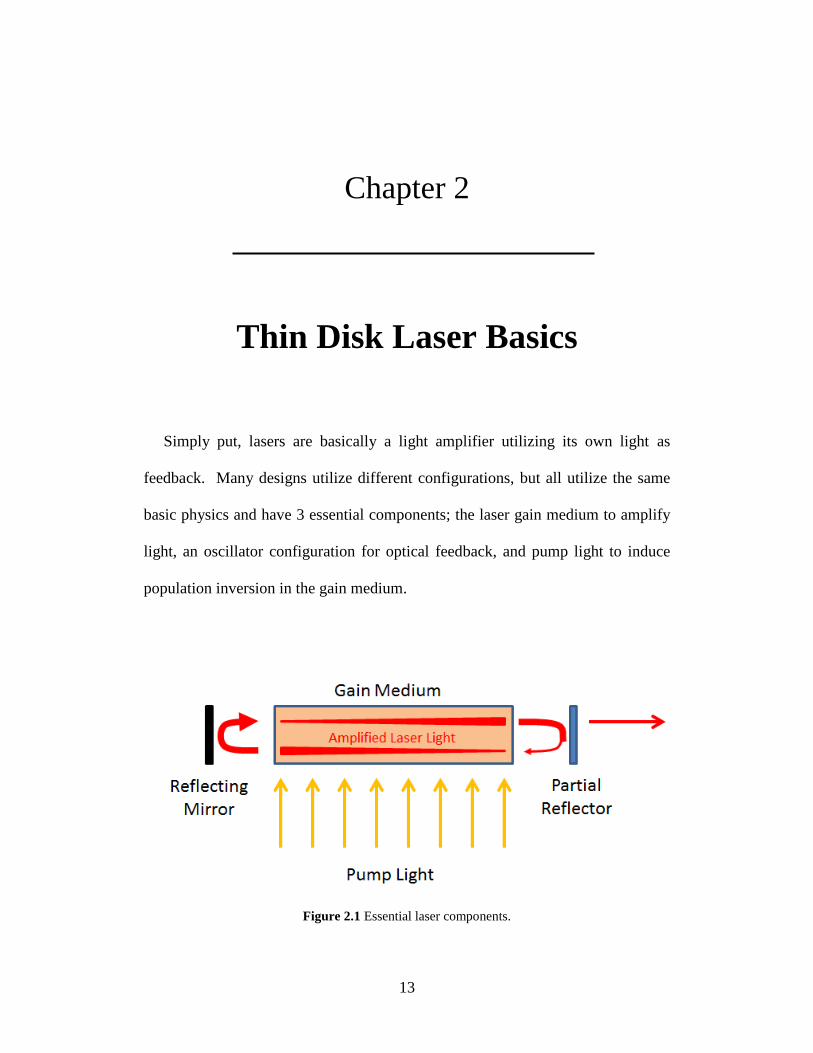
Simply put, lasers are basically a light amplifier utilizing its own light as
feedback. Many designs utilize different configurations, but all utilize the same
basic physics and have 3 essential components; the laser gain medium to amplify
light, an oscillator configuration for optical feedback, and pump light to induce
population inversion in the gain medium.
Figure 2.1 Essential laser components.
14
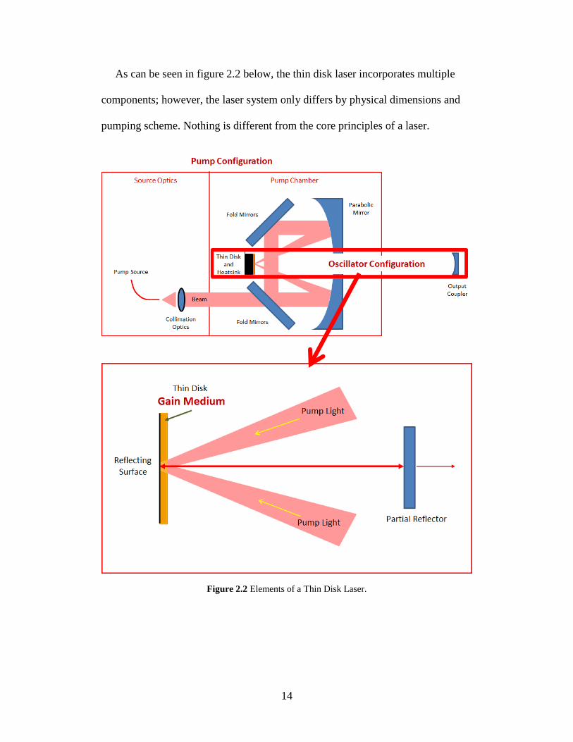
As can be seen in figure 2.2 below, the thin disk laser incorporates multiple
components; however, the laser system only differs by physical dimensions and
pumping scheme. Nothing is different from the core principles of a laser.
Figure 2.2 Elements of a Thin Disk Laser.

15
2.1 Laser Gain Medium
The laser gain medium is a collection of atoms, molecules, ions, or
semiconductor electrons. These can take the form of liquids such as organic dye
rhodamine 6G, gasses such as the Helium Neon, atoms doped in a host crystal
such as Nd:YAG, or semiconductor form such as Gallium Arsenide. For the thin
disk laser design, the amplifying gain medium is atoms doped in a glass/crystal
matrix. This is considered a solid-state system in this configuration.
Amplifying Atoms
Figure 2.3 Doping atoms in a host material.
Generally, in a solid-state laser’s gain medium, trivalent rare earth atoms such
as Ytterbium3+
, Erbium3+
, or Neodymium3+
(in this thesis, Thulium3+
) are doped
inside a host material such as such as Sapphire, Silica or YAG (in this thesis,
Germanate). The doped atoms enable the crystal to amplify light through the
process of stimulated absorption and emission, with each type of atom having
excited state transitions determined by the quantum nature of the doped atom.
Rare earth atoms are generally used because the electrons in the partially filled 4F
shell can be raised to unoccupied 4F levels by absorption of light.
16
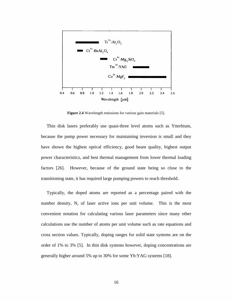
Figure 2.4 Wavelength emissions for various gain materials [5].
Thin disk lasers preferably use quasi-three level atoms such as Ytterbium,
because the pump power necessary for maintaining inversion is small and they
have shown the highest optical efficiency, good beam quality, highest output
power characteristics, and best thermal management from lower thermal loading
factors [26]. However, because of the ground state being so close to the
transitioning state, it has required large pumping powers to reach threshold.
Typically, the doped atoms are reported as a percentage paired with the
number density, N, of laser active ions per unit volume. This is the most
convenient notation for calculating various laser parameters since many other
calculations use the number of atoms per unit volume such as rate equations and
cross section values. Typically, doping ranges for solid state systems are on the
order of 1% to 3% [5]. In thin disk systems however, doping concentrations are
generally higher around 5% up to 30% for some Yb:YAG systems [18].

17
Host Material
The host material, in which the amplifying atoms are doped in, is used as a
means to fix the doping atoms in various configurations and densities in space.
The host crystal usually consists of a highly transparent material associated with
the absorption and emission wavelength of the doped atoms. Typically, it’s
uniformly homogenous and depending on the application, the doped atoms can be
doped with various percentage levels to influence laser beam output
characteristics.
As mentioned earlier, doping levels are usually higher in thin disk systems and
the host needs to be able to support the higher doped levels. Properties of the host
crystal need to encompass multiple characteristics such as hardness, damage
threshold, polarization, and solubility. As seen in the chart below, the host
material has an effect on the doping atoms by influencing the wavelength,
bandwidth, absorption and emission cross sections, radiative lifetimes, and non-
radiative transitions.
Table 2.1 Effects of different host materials using Thulium3+
[2].
18
2.2 Laser Oscillator
The laser oscillator is the configuration in which mirrors return light to enable
amplification of the laser signal and also determine resonator modes. As a bare
minimum, two mirror surfaces are needed; a highly reflective surface and a
partially reflective surface. The high reflection’s purpose is to reflect internal
resonating light back for amplification at minimal losses so higher laser output is
achieved. The partially reflecting mirror, commonly referred to as an output
coupler, is used to allow some of the laser light to escape the system while the
reflected light is sent back into the resonator to be amplified again. Eventually,
the laser’s amplification and internal losses from the mirrors reach an equilibrium
point and the escaped laser light becomes a steady beam output.
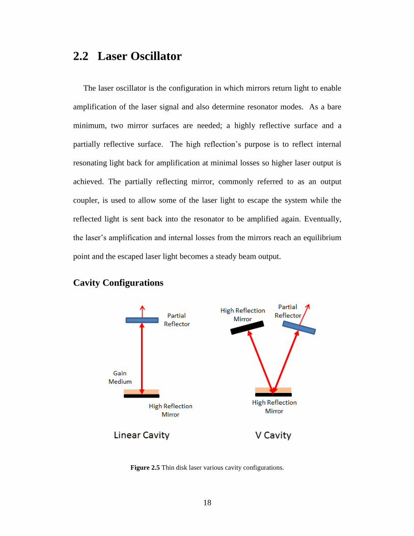
Cavity Configurations
Figure 2.5 Thin disk laser various cavity configurations.

19
In a thin disk laser, two cavity configurations are used; the linear cavity
configuration and the V-cavity configuration. In a linear cavity, the laser signal
resonates back and forth along the axis of the laser system and has a double pass
through the gain medium for each round trip. In a V-cavity configuration, a
separate end reflector is used causing the beam to be decoupled from the high
reflection side of the thin disk. In this configuration, the beam passes four times
through the gain medium per round trip, which gives the most amplification per
resonating loop. Both configurations can be used to stack several thin disk
modules to achieve high amplification and output powers.
Figure 2.6 Example of thin disk module stacking for high output power.
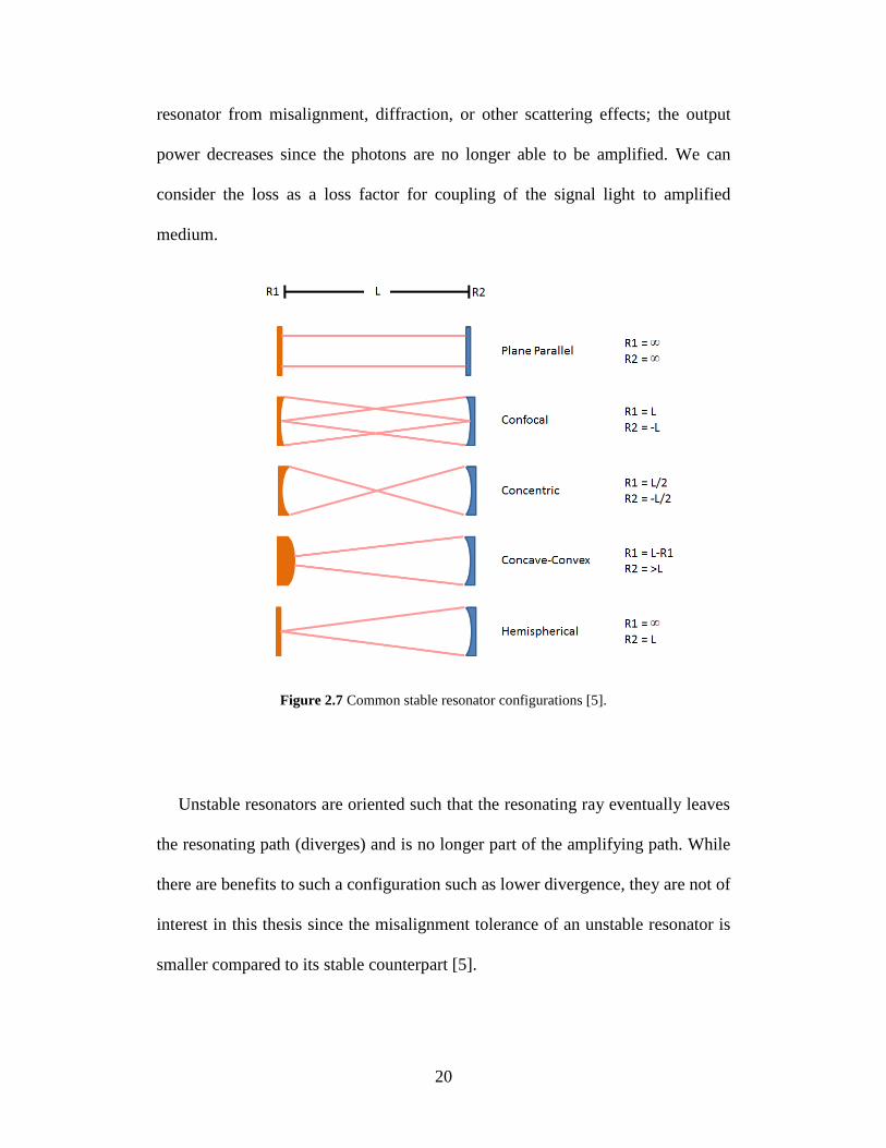
Resonator Types
There are two types of laser resonators; a stable resonator and an unstable
resonator. Stable resonators are described as the resonator mirror configuration
that allows the resonating ray to continuously stay in the cavity. These two
mirrors essentially couple the oscillating Gaussian wave so the signal light is
continuously amplified. If a small portion of the photons are lost out of the
20
resonator from misalignment, diffraction, or other scattering effects; the output
power decreases since the photons are no longer able to be amplified. We can
consider the loss as a loss factor for coupling of the signal light to amplified
medium.
Figure 2.7 Common stable resonator configurations [5].
Unstable resonators are oriented such that the resonating ray eventually leaves
the resonating path (diverges) and is no longer part of the amplifying path. While
there are benefits to such a configuration such as lower divergence, they are not of
interest in this thesis since the misalignment tolerance of an unstable resonator is
smaller compared to its stable counterpart [5].

21
2.3 Pumping Configuration
The pumping configuration is used as a means to send pump light into the gain
medium. Sources can take the form of flash lamps, seed laser systems, or diode
emitted lasers. In the case of the thin disk laser, one laser source is used in
combination with other optics to focus one beam into multiple overlapped beams
to increase power on the thin disk.
Figure 2.8 Thin disk pump scheme using Non-Sequential Zemax.
Source
Optics
Pump
Chamber
22
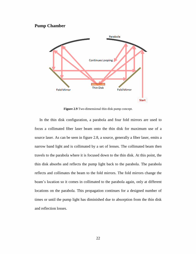
Pump Chamber
Figure 2.9 Two-dimensional thin disk pump concept.
In the thin disk configuration, a parabola and four fold mirrors are used to
focus a collimated fiber laser beam onto the thin disk for maximum use of a
source laser. As can be seen in figure 2.8, a source, generally a fiber laser, emits a
narrow band light and is collimated by a set of lenses. The collimated beam then
travels to the parabola where it is focused down to the thin disk. At this point, the
thin disk absorbs and reflects the pump light back to the parabola. The parabola
reflects and collimates the beam to the fold mirrors. The fold mirrors change the
beam’s location so it comes in collimated to the parabola again, only at different
locations on the parabola. This propagation continues for a designed number of
times or until the pump light has diminished due to absorption from the thin disk
and reflection losses.
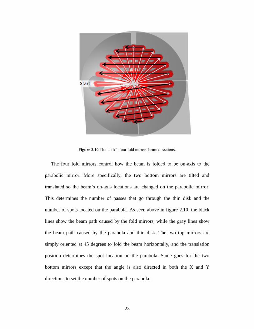
23
Figure 2.10 Thin disk’s four fold mirrors beam directions.
The four fold mirrors control how the beam is folded to be on-axis to the
parabolic mirror. More specifically, the two bottom mirrors are tilted and
translated so the beam’s on-axis locations are changed on the parabolic mirror.
This determines the number of passes that go through the thin disk and the
number of spots located on the parabola. As seen above in figure 2.10, the black
lines show the beam path caused by the fold mirrors, while the gray lines show
the beam path caused by the parabola and thin disk. The two top mirrors are
simply oriented at 45 degrees to fold the beam horizontally, and the translation
position determines the spot location on the parabola. Same goes for the two
bottom mirrors except that the angle is also directed in both the X and Y
directions to set the number of spots on the parabola.

24
Source Optics
Figure 2.11 Source optics into pump chamber.
An initial pump source is used in combination with collimating optics before
projecting into the pump chamber. For the thin disk laser, compact systems use
fiber diode lasers; however other ‘seed’ lasers can be used to send a specific laser
into the gain medium. The collimation optics can be as simple as a single lens, or
can be a combination of lenses for alignment purposes or to minimize aberrations.
In compact thin disk systems (shown in figure 1.6), a fiber laser emits light to a
lens where the light is then collimated to two additional lenses. The additional
lenses are typically used for alignment purposes such as accurate translation of the
incoming beam and to possibly change magnification before entering the pump
chamber.
Pump Source (Fiber Laser)
Collimation Lens Additional
Lenses

25
Chapter 3
Laser Fundamentals and Modelling
Fundamentally, operation of a laser can be described and modeled from
absorption and emission processes. Detailed quantum models and specific
interaction effects of atoms are not required. As a basis, the only required
knowledge is that there are discrete energy levels between states of electrons in an
atom; and that each atom has its own allowed electron transition states defined by
the quantum numbers associated with the atom. These electrons can be excited to
higher energy levels by absorption through various excitation processes, and then
transition back down to lower energy levels by the emission of photons through
spontaneous emission, stimulated emission or other quantum mechanical
phenomenon.
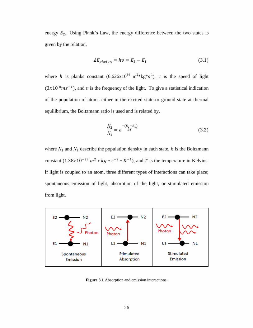
3.1 Light Interactions
Simply, a two level energy diagram can be used to describe the multi-level
states in an atom; a ground state |1⟩ with energy 𝐸1, and an excited state |2⟩ with
26
energy 𝐸2,. Using Plank’s Law, the energy difference between the two states is
given by the relation,
𝛥𝐸𝑝ℎ𝑜𝑡𝑜𝑛 = ℎ𝑣 = 𝐸2 − 𝐸1 (3.1)
where ℎ is planks constant (6.626x1034
m2*kg*s
-1), 𝑐 is the speed of light
(3𝑥10 8𝑚𝑠−1), and 𝑣 is the frequency of the light. To give a statistical indication
of the population of atoms either in the excited state or ground state at thermal
equilibrium, the Boltzmann ratio is used and is related by,
𝑁2
𝑁1= 𝑒
−(𝐸2−𝐸1)𝑘𝑇 (3.2)
where 𝑁1 and 𝑁2 describe the population density in each state, 𝑘 is the Boltzmann
constant (1.38𝑥10−23 𝑚2 ∗ 𝑘𝑔 ∗ 𝑠−2 ∗ 𝐾−1), and 𝑇 is the temperature in Kelvins.
If light is coupled to an atom, three different types of interactions can take place;
spontaneous emission of light, absorption of the light, or stimulated emission
from light.
Figure 3.1 Absorption and emission interactions.
27
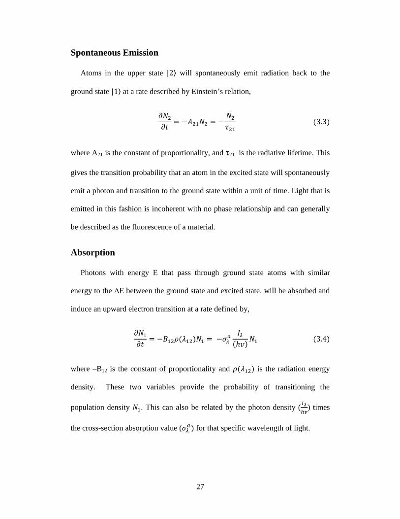
Spontaneous Emission
Atoms in the upper state |2⟩ will spontaneously emit radiation back to the
ground state |1⟩ at a rate described by Einstein’s relation,
𝜕𝑁2
𝜕𝑡= −𝐴21𝑁2 = −
𝑁2
𝜏21 (3.3)
where A21 is the constant of proportionality, and τ21 is the radiative lifetime. This
gives the transition probability that an atom in the excited state will spontaneously
emit a photon and transition to the ground state within a unit of time. Light that is
emitted in this fashion is incoherent with no phase relationship and can generally
be described as the fluorescence of a material.
Absorption
Photons with energy E that pass through ground state atoms with similar
energy to the ΔE between the ground state and excited state, will be absorbed and
induce an upward electron transition at a rate defined by,
𝜕𝑁1
𝜕𝑡= −𝐵12𝜌(𝜆12)𝑁1 = −𝜎𝜆
𝑎 𝐼𝜆(ℎ𝑣)
𝑁1 (3.4)
where –B12 is the constant of proportionality and 𝜌(𝜆12) is the radiation energy
density. These two variables provide the probability of transitioning the
population density 𝑁1. This can also be related by the photon density (𝐼𝜆
ℎ𝑣) times
the cross-section absorption value (𝜎𝜆𝑎) for that specific wavelength of light.
28
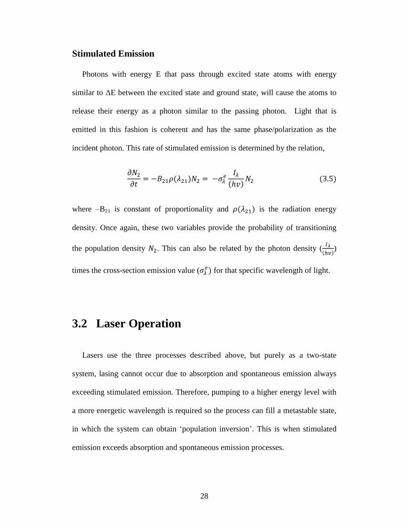
Stimulated Emission
Photons with energy E that pass through excited state atoms with energy
similar to ΔE between the excited state and ground state, will cause the atoms to
release their energy as a photon similar to the passing photon. Light that is
emitted in this fashion is coherent and has the same phase/polarization as the
incident photon. This rate of stimulated emission is determined by the relation,
𝜕𝑁2
𝜕𝑡= −𝐵21𝜌(𝜆21)𝑁2 = −𝜎𝜆
𝑒 𝐼𝜆(ℎ𝑣)
𝑁2 (3.5)
where –B21 is constant of proportionality and 𝜌(𝜆21) is the radiation energy
density. Once again, these two variables provide the probability of transitioning
the population density 𝑁2. This can also be related by the photon density (𝐼𝜆
(ℎ𝑣))
times the cross-section emission value (𝜎𝜆𝑒) for that specific wavelength of light.
3.2 Laser Operation
Lasers use the three processes described above, but purely as a two-state
system, lasing cannot occur due to absorption and spontaneous emission always
exceeding stimulated emission. Therefore, pumping to a higher energy level with
a more energetic wavelength is required so the process can fill a metastable state,
in which the system can obtain ‘population inversion’. This is when stimulated
emission exceeds absorption and spontaneous emission processes.

29
Three Level System
Figure 3.2 Three level diagram of Thulium.
For Thulium, the energy level diagram is considered a three-level system,
which is simplified to a ground state |1⟩, a metastable state |2⟩, and a pumping
state |3⟩. In this scheme, pump light 𝐼𝑝 incident on the gain medium is absorbed
𝑎 and emitted 𝑒 at a value determined by the cross-section σ of the gain material.
The absorbed power transitions atoms to state |3⟩, where it then transitions very
fast into state |2⟩ at a rate defined by τ32. At this point, atoms in state |2⟩
transition to state |1⟩ by emitting photons as stimulated emission of the signal
light 𝐼𝑠 or as spontaneous emission at a rate defined by τ21. Also, a portion of the
signal light is re-absorbed. Lasing begins once the signal light is emitted as
stimulated radiation and exceeds absorption and spontaneous processes. In a
three-level system,
𝑁1 + 𝑁2 + 𝑁3 = 𝑁𝑡 (3.6)

30
Combining the three light interaction rates and using the figure 3.2 above, the
total population rate change in each state is given by,
(𝜕𝑁
𝜕𝑡) = (
𝜕𝑁
𝜕𝑡)𝑆𝑡𝑖𝑚𝑢𝑙𝑎𝑡𝑒𝑑𝐴𝑏𝑠𝑜𝑟𝑝𝑡𝑖𝑜𝑛
+ (𝜕𝑁
𝜕𝑡)
𝑆𝑡𝑖𝑚𝑢𝑙𝑎𝑡𝑒𝑑𝐸𝑚𝑖𝑠𝑠𝑖𝑜𝑛
+ (𝜕𝑁
𝜕𝑡)
𝑆𝑝𝑜𝑛𝑡𝑎𝑛𝑒𝑜𝑢𝑠𝐸𝑚𝑖𝑠𝑠𝑖𝑜𝑛
(3.7)
Therefore for state |1⟩,
𝑁1(𝑥, 𝑦, 𝑧, 𝑡)
𝜕𝑡=
𝐼𝑝(𝑥, 𝑦, 𝑧, 𝑡)
ℎ𝑣𝑝[𝜎𝑝
𝑒(𝑇)𝑁3(𝑥, 𝑦, 𝑧, 𝑡) − 𝜎𝑝𝑎(𝑇)𝑁1(𝑥, 𝑦, 𝑧, 𝑡)] + ⋯
…+𝐼𝑠(𝑥, 𝑦, 𝑧, 𝑡)
ℎ𝑣𝑠
[𝜎𝑠𝑒(𝑇)𝑁2(𝑥, 𝑦, 𝑧, 𝑡) − 𝜎𝑠
𝑎(𝑇)𝑁1(𝑥, 𝑦, 𝑧, 𝑡)] + ⋯
+𝑁2(𝑥, 𝑦, 𝑧, 𝑡)
𝜏21 (3.8)
State |2⟩,
𝑁2(𝑥, 𝑦, 𝑧, 𝑡)
𝜕𝑡=
𝑁3(𝑥, 𝑦, 𝑧, 𝑡)
𝜏32−
𝑁2(𝑥, 𝑦, 𝑧, 𝑡)
𝜏21+ ⋯
…+𝐼𝑠(𝑥, 𝑦, 𝑧, 𝑡)
ℎ𝑣𝑠
[𝜎𝑠𝑒(𝑇)𝑁2(𝑥, 𝑦, 𝑧, 𝑡) − 𝜎𝑠
𝑎(𝑇)𝑁1(𝑥, 𝑦, 𝑧, 𝑡)] (3.9)
State |3⟩,
𝑁3(𝑥, 𝑦, 𝑧, 𝑡)
𝜕𝑡=
𝐼𝑝(𝑥, 𝑦, 𝑧, 𝑡)
ℎ𝑣𝑝[𝜎𝑝
𝑒(𝑇)𝑁3(𝑥, 𝑦, 𝑧, 𝑡) − 𝜎𝑝𝑎(𝑇)𝑁1(𝑥, 𝑦, 𝑧, 𝑡)] + ⋯
…−𝑁3(𝑥, 𝑦, 𝑧, 𝑡)
𝜏32 (3.10)
31
Laser Assumptions
In a real dynamic laser system, the doped atoms and population densities in the
gain medium will vary in space and change with time 𝑁1(𝑥, 𝑦, 𝑧, 𝑡), as well as the
irradiance of the pump/signal light will vary with space and change with time
𝐼(𝑥, 𝑦, 𝑧, 𝑡). The cross section values are dependent on the spatial profile from a
temperature 𝑇 variation inside the gain medium that is caused from the previous
two effects. To simplify the equations from complex phenomenon and
mathematics, the following assumptions are made.
Top-Hat Pump Laser – This assumption removes the spatial dependence
of the irradiance profile. In a multi-mode fiber, the output beam does not
follow a purely Gaussian beam since many modes are part of the output.
Homogenous and Uniformly Doped Gain Medium – This assumption
(with a top-hat pump), removes the spatial dependence of the population
states.
Constant Temperature Cross-Section – Since the thin disk uses a very thin
gain medium and is heatsinked, it is assumed that the heat across the thin
disk is uniform and is efficiently extracted out of the disk to maintain a
constant temperature value.
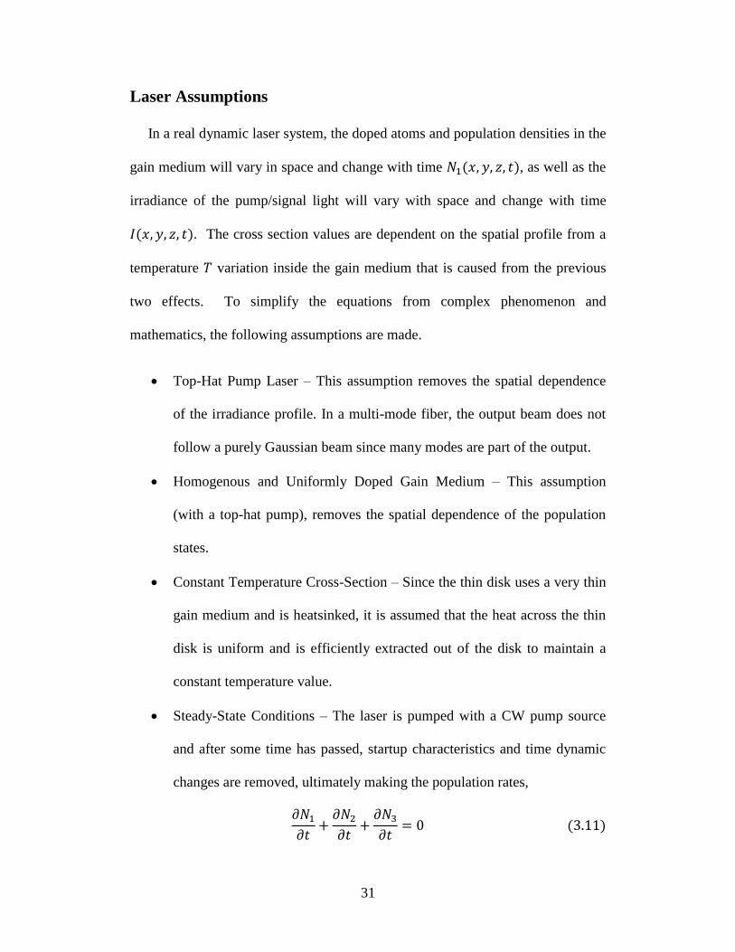
Steady-State Conditions – The laser is pumped with a CW pump source
and after some time has passed, startup characteristics and time dynamic
changes are removed, ultimately making the population rates,
𝜕𝑁1
𝜕𝑡+
𝜕𝑁2
𝜕𝑡+
𝜕𝑁3
𝜕𝑡= 0 (3.11)
32
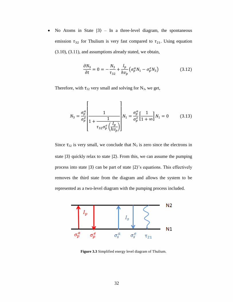
No Atoms in State |3⟩ – In a three-level diagram, the spontaneous
emission 𝜏32 for Thulium is very fast compared to 𝜏21. Using equation
(3.10), (3.11), and assumptions already stated, we obtain,
𝜕𝑁3
𝜕𝑡= 0 = −
𝑁3
𝜏32+
𝐼𝑝
ℎ𝑣𝑝(𝜎𝑝
𝑎𝑁1 − 𝜎𝑝𝑒𝑁3) (3.12)
Therefore, with τ32 very small and solving for N3, we get,
𝑁3 =𝜎𝑝
𝑎
𝜎𝑝𝑒
[
1
1 +1
𝜏32𝜎𝑝𝑒 (
𝐼𝑝ℎ𝑣𝑝
)]
𝑁1 =𝜎𝑝
𝑎
𝜎𝑝𝑒 [
1
1 + ∞]𝑁1 = 0 (3.13)
Since τ32 is very small, we conclude that N3 is zero since the electrons in
state |3⟩ quickly relax to state |2⟩. From this, we can assume the pumping
process into state |3⟩ can be part of state |2⟩’s equations. This effectively
removes the third state from the diagram and allows the system to be
represented as a two-level diagram with the pumping process included.
Figure 3.3 Simplified energy level diagram of Thulium.
33
3.3 Rate Equations
Population Rate Equations
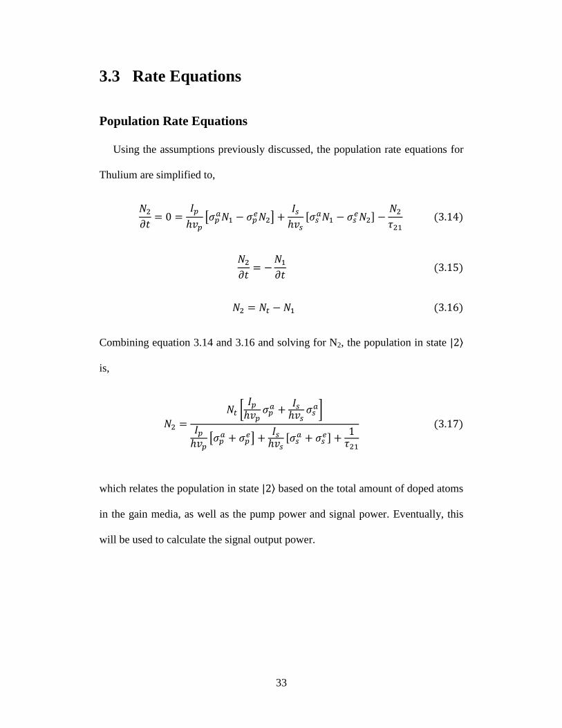
Using the assumptions previously discussed, the population rate equations for
Thulium are simplified to,
𝑁2
𝜕𝑡= 0 =
𝐼𝑝
ℎ𝑣𝑝[𝜎𝑝
𝑎𝑁1 − 𝜎𝑝𝑒𝑁2] +
𝐼𝑠ℎ𝑣𝑠
[𝜎𝑠𝑎𝑁1 − 𝜎𝑠
𝑒𝑁2] −𝑁2
𝜏21 (3.14)
𝑁2
𝜕𝑡= −
𝑁1
𝜕𝑡 (3.15)
𝑁2 = 𝑁𝑡 − 𝑁1 (3.16)
Combining equation 3.14 and 3.16 and solving for N2, the population in state |2⟩
is,
𝑁2 =
𝑁𝑡 [𝐼𝑝
ℎ𝑣𝑝𝜎𝑝
𝑎 +𝐼𝑠
ℎ𝑣𝑠𝜎𝑠
𝑎]
𝐼𝑝ℎ𝑣𝑝
[𝜎𝑝𝑎 + 𝜎𝑝
𝑒] +𝐼𝑠
ℎ𝑣𝑠[𝜎𝑠
𝑎 + 𝜎𝑠𝑒] +
1𝜏21
(3.17)
which relates the population in state |2⟩ based on the total amount of doped atoms
in the gain media, as well as the pump power and signal power. Eventually, this
will be used to calculate the signal output power.
34
Photon Rate Equations
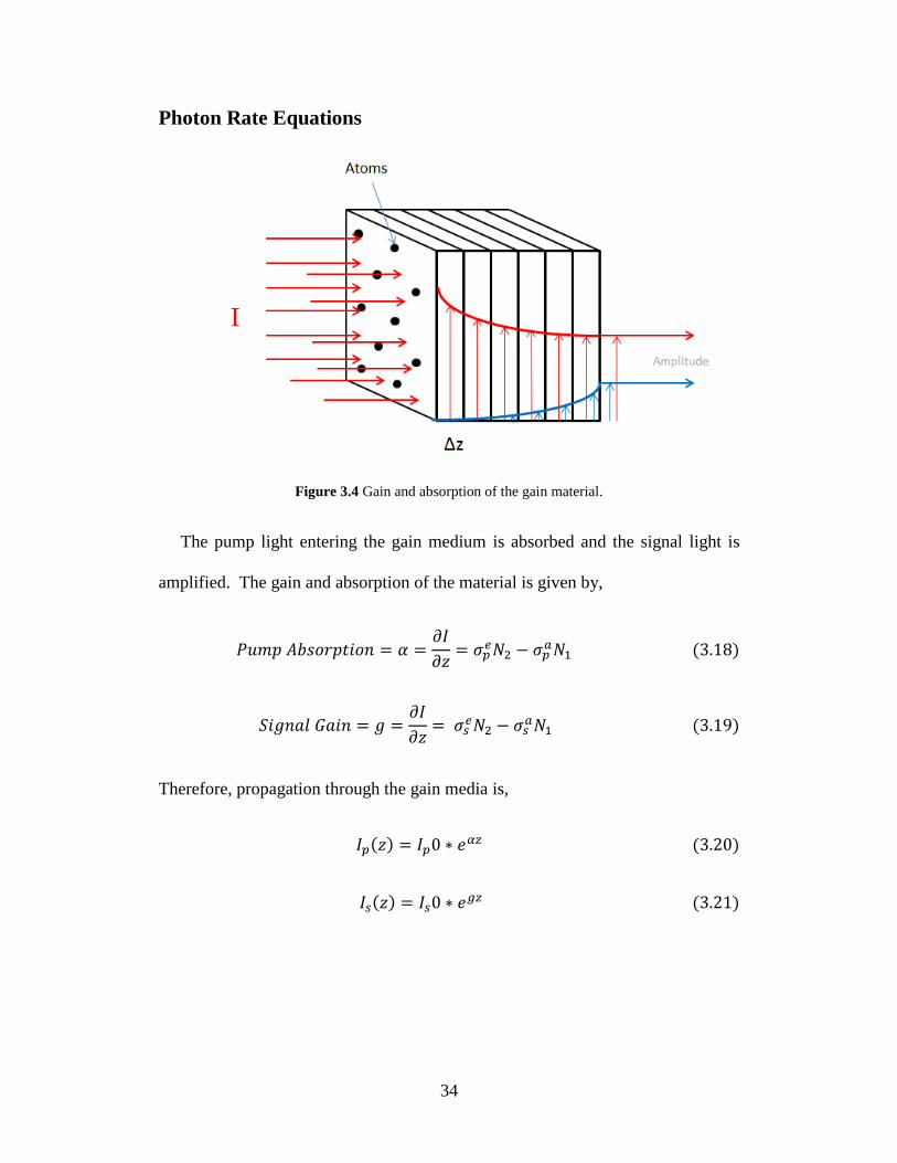
Figure 3.4 Gain and absorption of the gain material.
The pump light entering the gain medium is absorbed and the signal light is
amplified. The gain and absorption of the material is given by,
𝑃𝑢𝑚𝑝 𝐴𝑏𝑠𝑜𝑟𝑝𝑡𝑖𝑜𝑛 = 𝛼 =𝜕𝐼
𝜕𝑧= 𝜎𝑝
𝑒𝑁2 − 𝜎𝑝𝑎𝑁1 (3.18)
𝑆𝑖𝑔𝑛𝑎𝑙 𝐺𝑎𝑖𝑛 = 𝑔 =𝜕𝐼
𝜕𝑧= 𝜎𝑠
𝑒𝑁2 − 𝜎𝑠𝑎𝑁1 (3.19)
Therefore, propagation through the gain media is,
𝐼𝑝(𝑧) = 𝐼𝑝0 ∗ 𝑒𝛼𝑧 (3.20)
𝐼𝑠(𝑧) = 𝐼𝑠0 ∗ 𝑒𝑔𝑧 (3.21)
35
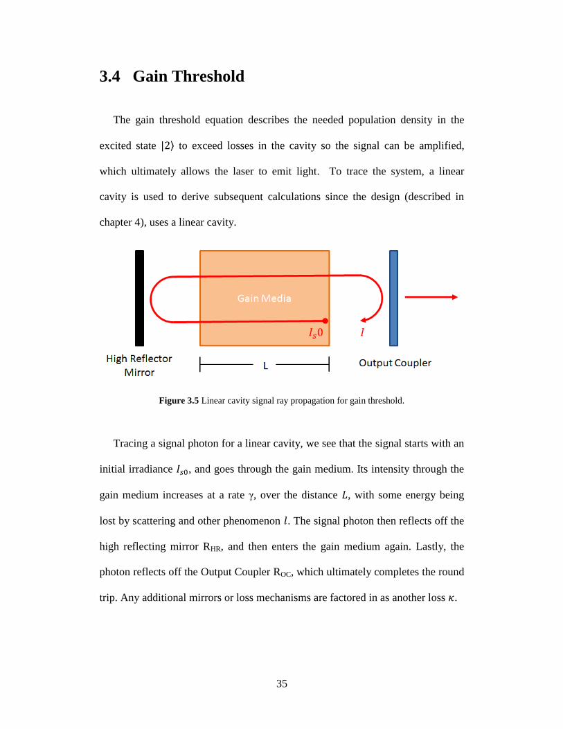
3.4 Gain Threshold
The gain threshold equation describes the needed population density in the
excited state |2⟩ to exceed losses in the cavity so the signal can be amplified,
which ultimately allows the laser to emit light. To trace the system, a linear
cavity is used to derive subsequent calculations since the design (described in
chapter 4), uses a linear cavity.
Figure 3.5 Linear cavity signal ray propagation for gain threshold.
Tracing a signal photon for a linear cavity, we see that the signal starts with an
initial irradiance 𝐼𝑠0, and goes through the gain medium. Its intensity through the
gain medium increases at a rate γ, over the distance 𝐿, with some energy being
lost by scattering and other phenomenon 𝑙. The signal photon then reflects off the
high reflecting mirror RHR, and then enters the gain medium again. Lastly, the
photon reflects off the Output Coupler ROC, which ultimately completes the round
trip. Any additional mirrors or loss mechanisms are factored in as another loss 𝜅.
36
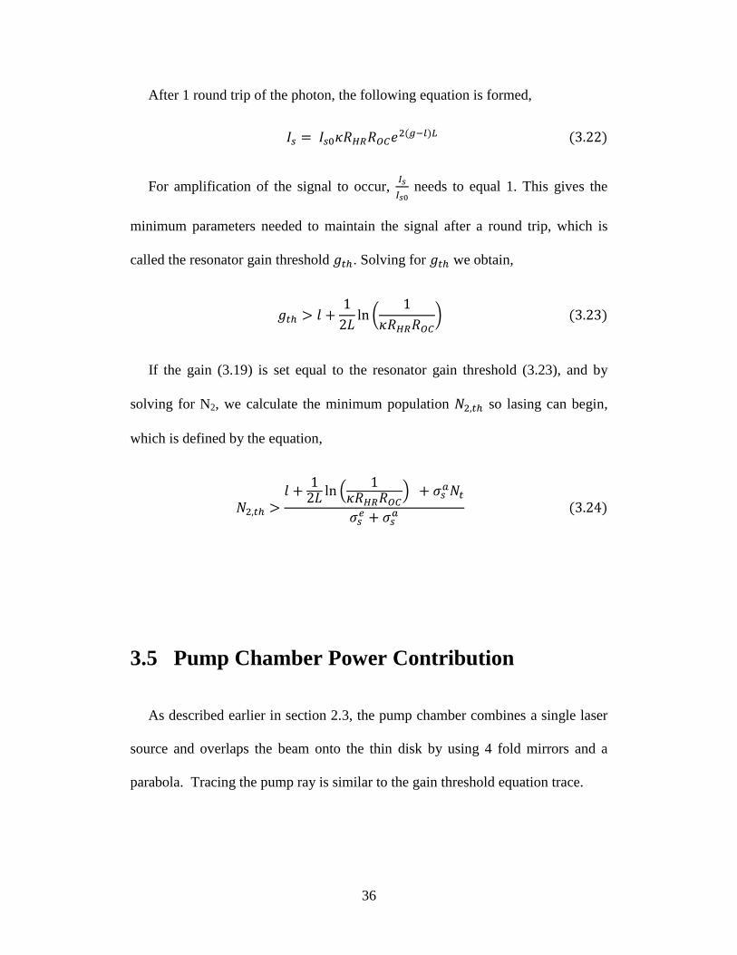
After 1 round trip of the photon, the following equation is formed,
𝐼𝑠 = 𝐼𝑠0𝜅𝑅𝐻𝑅𝑅𝑂𝐶𝑒2(𝑔−𝑙)𝐿 (3.22)
For amplification of the signal to occur, 𝐼𝑠
𝐼𝑠0 needs to equal 1. This gives the
minimum parameters needed to maintain the signal after a round trip, which is
called the resonator gain threshold 𝑔𝑡ℎ. Solving for 𝑔𝑡ℎ we obtain,
𝑔𝑡ℎ > 𝑙 +1
2𝐿ln (
1
𝜅𝑅𝐻𝑅𝑅𝑂𝐶) (3.23)
If the gain (3.19) is set equal to the resonator gain threshold (3.23), and by
solving for N2, we calculate the minimum population 𝑁2,𝑡ℎ so lasing can begin,
which is defined by the equation,
𝑁2,𝑡ℎ >𝑙 +
12𝐿 ln (
1𝜅𝑅𝐻𝑅𝑅𝑂𝐶
) + 𝜎𝑠𝑎𝑁𝑡
𝜎𝑠𝑒 + 𝜎𝑠
𝑎 (3.24)
3.5 Pump Chamber Power Contribution
As described earlier in section 2.3, the pump chamber combines a single laser
source and overlaps the beam onto the thin disk by using 4 fold mirrors and a
parabola. Tracing the pump ray is similar to the gain threshold equation trace.

37
Figure 3.6 Associated pump power losses as the beam folds around the pump chamber.
The beam has an initial power ϕp0 and reflects off the parabola with reflectance
𝑃. The light then focuses to the thin disk where the gain medium absorbs the light
𝑒𝑎𝐿, where 𝐿 is the length of the gain material. The light then reflects off a high
reflection coating 𝑅𝐻𝑅 on the backside of the thin disk to once again be absorbed
𝑒𝑎𝐿 in the gain medium. The light then continues to the parabola experiencing a
reflection loss 𝑃 again and reflection losses from the folding mirrors 𝐹. This
continues looping around a number of times determined by the number of desired
number of passes through the thin disk.
In this configuration, the pump experiences a ‘double pass’, since the light
passes through the gain medium twice in nearly the same location. The total
energy through the gain medium is assumed constant since the length 𝐿 is very
small, which makes the total pump energy nearly even throughout the length of
the disk. The incident power through the thin disk is considered ‘forward’ light
and the power after the thin disk is considered ‘backwards’ light.
38
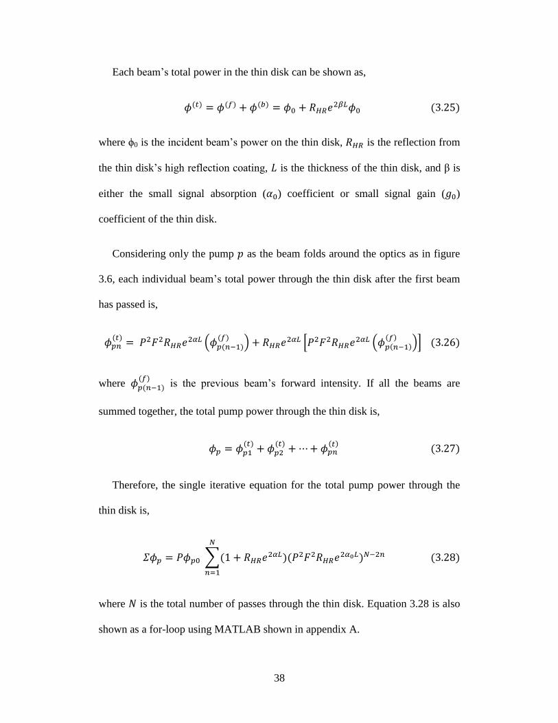
Each beam’s total power in the thin disk can be shown as,
𝜙(𝑡) = 𝜙(𝑓) + 𝜙(𝑏) = 𝜙0 + 𝑅𝐻𝑅𝑒2𝛽𝐿𝜙0 (3.25)
where ϕ0 is the incident beam’s power on the thin disk, 𝑅𝐻𝑅 is the reflection from
the thin disk’s high reflection coating, 𝐿 is the thickness of the thin disk, and β is
either the small signal absorption (𝛼0) coefficient or small signal gain (𝑔0)
coefficient of the thin disk.
Considering only the pump 𝑝 as the beam folds around the optics as in figure
3.6, each individual beam’s total power through the thin disk after the first beam
has passed is,
𝜙𝑝𝑛(𝑡)
= 𝑃2𝐹2𝑅𝐻𝑅𝑒2𝛼𝐿 (𝜙𝑝(𝑛−1)(𝑓)
) + 𝑅𝐻𝑅𝑒2𝛼𝐿 [𝑃2𝐹2𝑅𝐻𝑅𝑒2𝛼𝐿 (𝜙𝑝(𝑛−1)(𝑓)
)] (3.26)
where 𝜙𝑝(𝑛−1)(𝑓)
is the previous beam’s forward intensity. If all the beams are
summed together, the total pump power through the thin disk is,
𝜙𝑝 = 𝜙𝑝1(𝑡)
+ 𝜙𝑝2(𝑡)
+ ⋯+ 𝜙𝑝𝑛(𝑡) (3.27)
Therefore, the single iterative equation for the total pump power through the
thin disk is,
𝛴𝜙𝑝 = 𝑃𝜙𝑝0 ∑(1 + 𝑅𝐻𝑅𝑒2𝛼𝐿)(𝑃2𝐹2𝑅𝐻𝑅𝑒2𝛼0𝐿)𝑁−2𝑛
𝑁
𝑛=1
(3.28)
where 𝑁 is the total number of passes through the thin disk. Equation 3.28 is also
shown as a for-loop using MATLAB shown in appendix A.
39
3.6 Resonator Effects
As mentioned earlier in section 2.2.2, the laser output power decreases when
the coupling efficiency between the signal and pump decreases. Therefore, an
understanding of the resonator’s effects on the system must be included in any
model.
Signal Aperture Effect
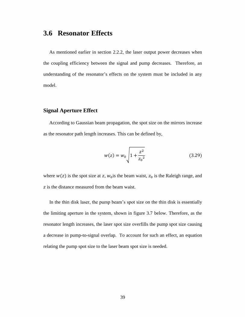
According to Gaussian beam propagation, the spot size on the mirrors increase
as the resonator path length increases. This can be defined by,
𝑤(𝑧) = 𝑤0√1 +𝑧2
𝑧02 (3.29)
where 𝑤(𝑧) is the spot size at 𝑧, 𝑤0is the beam waist, 𝑧0 is the Raleigh range, and
𝑧 is the distance measured from the beam waist.
In the thin disk laser, the pump beam’s spot size on the thin disk is essentially
the limiting aperture in the system, shown in figure 3.7 below. Therefore, as the
resonator length increases, the laser spot size overfills the pump spot size causing
a decrease in pump-to-signal overlap. To account for such an effect, an equation
relating the pump spot size to the laser beam spot size is needed.
40
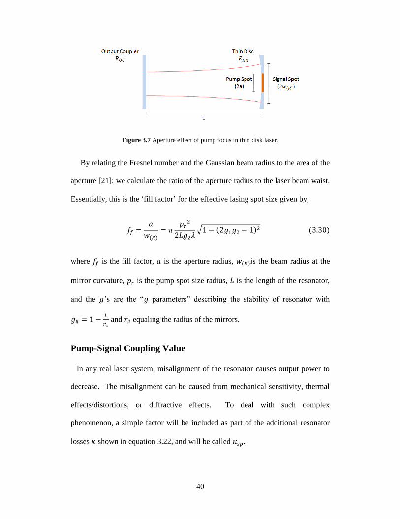
Figure 3.7 Aperture effect of pump focus in thin disk laser.
By relating the Fresnel number and the Gaussian beam radius to the area of the
aperture [21]; we calculate the ratio of the aperture radius to the laser beam waist.
Essentially, this is the ‘fill factor’ for the effective lasing spot size given by,
𝑓𝑓 =𝑎
𝑤(𝑅)= 𝜋
𝑝𝑟2
2𝐿𝑔2𝜆√1 − (2𝑔1𝑔2 − 1)2 (3.30)
where 𝑓𝑓 is the fill factor, 𝑎 is the aperture radius, 𝑤(𝑅)is the beam radius at the
mirror curvature, 𝑝𝑟 is the pump spot size radius, 𝐿 is the length of the resonator,
and the 𝑔’s are the “𝑔 parameters” describing the stability of resonator with
𝑔# = 1 −𝐿
𝑟# and 𝑟# equaling the radius of the mirrors.
Pump-Signal Coupling Value
In any real laser system, misalignment of the resonator causes output power to
decrease. The misalignment can be caused from mechanical sensitivity, thermal
effects/distortions, or diffractive effects. To deal with such complex
phenomenon, a simple factor will be included as part of the additional resonator
losses 𝜅 shown in equation 3.22, and will be called 𝜅𝑠𝑝.
41
3.7 CW Power Output Model
Output Power Equations
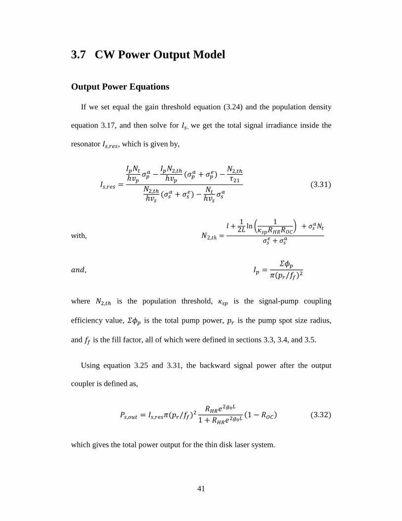
If we set equal the gain threshold equation (3.24) and the population density
equation 3.17, and then solve for 𝐼𝑠 , we get the total signal irradiance inside the
resonator 𝐼𝑠,𝑟𝑒𝑠, which is given by,
𝐼𝑠,𝑟𝑒𝑠 =
𝐼𝑝𝑁𝑡
ℎ𝑣𝑝𝜎𝑝
𝑎 −𝐼𝑝𝑁2,𝑡ℎ
ℎ𝑣𝑝(𝜎𝑝
𝑎 + 𝜎𝑝𝑒) −
𝑁2,𝑡ℎ
𝜏21
𝑁2,𝑡ℎ
ℎ𝑣𝑠(𝜎𝑠
𝑎 + 𝜎𝑠𝑒) −
𝑁𝑡
ℎ𝑣𝑠𝜎𝑠
𝑎 (3.31)
with, 𝑁2,𝑡ℎ =
𝑙 +12𝐿
ln (1
𝜅𝑠𝑝𝑅𝐻𝑅𝑅𝑂𝐶) + 𝜎𝑠
𝑎𝑁𝑡
𝜎𝑠𝑒 + 𝜎𝑠
𝑎
𝑎𝑛𝑑, 𝐼𝑝 =𝛴𝜙𝑝
𝜋(𝑝𝑟/𝑓𝑓)2
where 𝑁2,𝑡ℎ is the population threshold, 𝜅𝑠𝑝 is the signal-pump coupling
efficiency value, 𝛴𝜙𝑝 is the total pump power, 𝑝𝑟 is the pump spot size radius,
and 𝑓𝑓 is the fill factor, all of which were defined in sections 3.3, 3.4, and 3.5.
Using equation 3.25 and 3.31, the backward signal power after the output
coupler is defined as,
𝑃𝑠,𝑜𝑢𝑡 = 𝐼𝑠,𝑟𝑒𝑠𝜋(𝑝𝑟/𝑓𝑓)2
𝑅𝐻𝑅𝑒2𝑔0𝐿
1 + 𝑅𝐻𝑅𝑒2𝑔0𝐿(1 − 𝑅𝑂𝐶) (3.32)
which gives the total power output for the thin disk laser system.
42
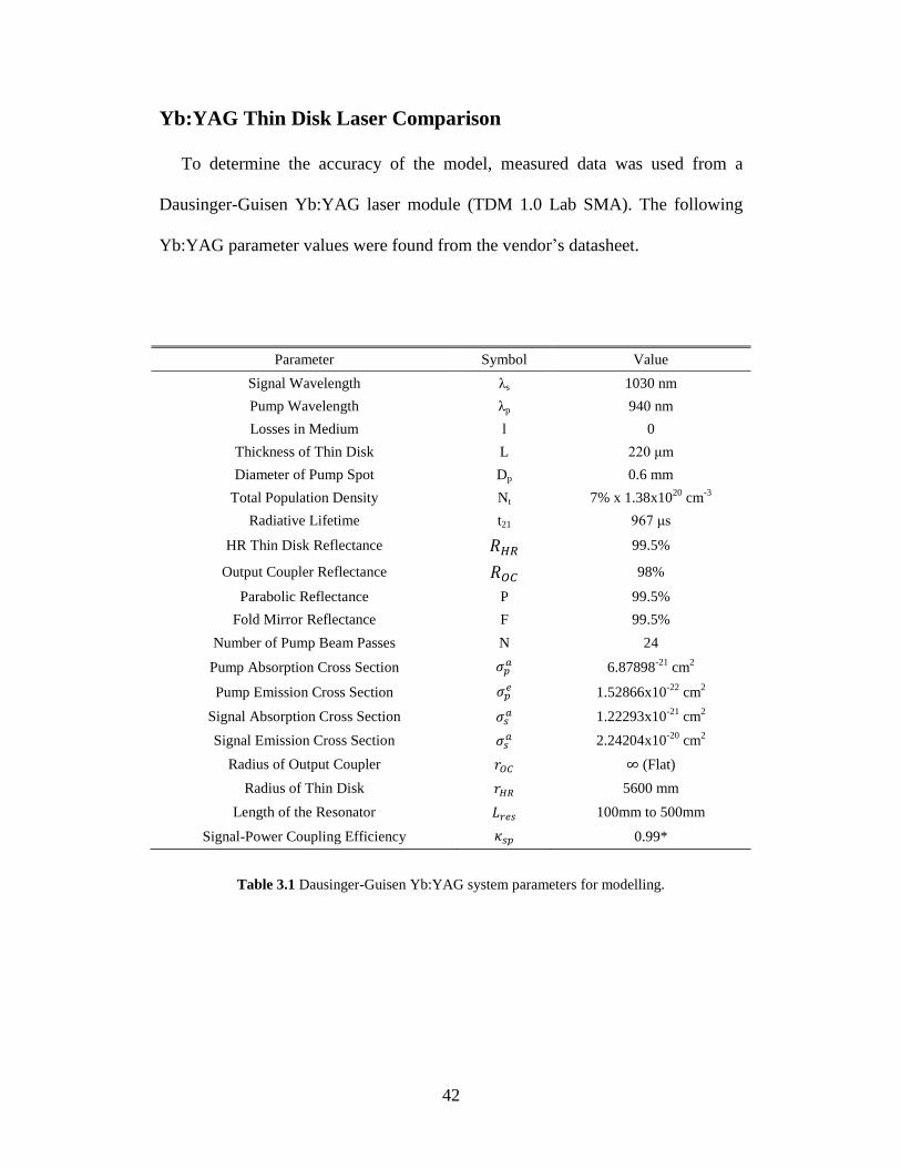
Yb:YAG Thin Disk Laser Comparison
To determine the accuracy of the model, measured data was used from a
Dausinger-Guisen Yb:YAG laser module (TDM 1.0 Lab SMA). The following
Yb:YAG parameter values were found from the vendor’s datasheet.
Parameter Symbol Value
Signal Wavelength λs 1030 nm
Pump Wavelength λp 940 nm
Losses in Medium l 0
Thickness of Thin Disk L 220 μm
Diameter of Pump Spot Dp 0.6 mm
Total Population Density Nt 7% x 1.38x10²⁰
cm-3
Radiative Lifetime t21 967 μs
HR Thin Disk Reflectance 𝑅𝐻𝑅 99.5%
Output Coupler Reflectance 𝑅𝑂𝐶 98%
Parabolic Reflectance P 99.5%
Fold Mirror Reflectance F 99.5%
Number of Pump Beam Passes N 24
Pump Absorption Cross Section 𝜎𝑝𝑎 6.87898
-21 cm
2
Pump Emission Cross Section 𝜎𝑝𝑒 1.52866x10
-22 cm
2
Signal Absorption Cross Section 𝜎𝑠𝑎 1.22293x10
-21 cm
2
Signal Emission Cross Section 𝜎𝑠𝑎 2.24204x10
-20 cm
2
Radius of Output Coupler 𝑟𝑂𝐶 ∞ (Flat)
Radius of Thin Disk 𝑟𝐻𝑅 5600 mm
Length of the Resonator 𝐿𝑟𝑒𝑠 100mm to 500mm
Signal-Power Coupling Efficiency 𝜅𝑠𝑝 0.99*
Table 3.1 Dausinger-Guisen Yb:YAG system parameters for modelling.
43
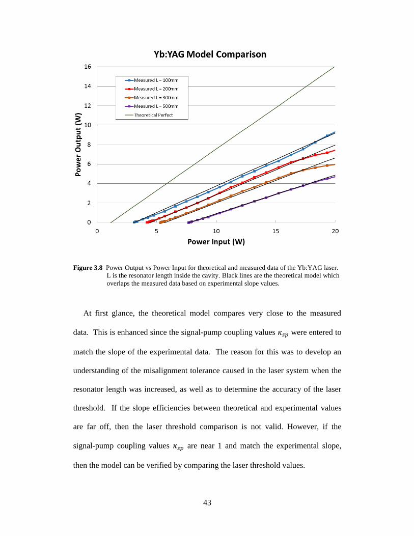
Figure 3.8 Power Output vs Power Input for theoretical and measured data of the Yb:YAG laser.
L is the resonator length inside the cavity. Black lines are the theoretical model which
overlaps the measured data based on experimental slope values.
At first glance, the theoretical model compares very close to the measured
data. This is enhanced since the signal-pump coupling values 𝜅𝑠𝑝 were entered to
match the slope of the experimental data. The reason for this was to develop an
understanding of the misalignment tolerance caused in the laser system when the
resonator length was increased, as well as to determine the accuracy of the laser
threshold. If the slope efficiencies between theoretical and experimental values
are far off, then the laser threshold comparison is not valid. However, if the
signal-pump coupling values 𝜅𝑠𝑝 are near 1 and match the experimental slope,
then the model can be verified by comparing the laser threshold values.

44
Resonator Length
Slope Efficiency
(Linear Regression of
Experimental Data)
Signal-Pump Coupling Values
(κsp)
(@Perfect Overlap) (0.853) (1.000)
100 mm 0.546 0.9885
200 mm 0.519 0.9868
300 mm 0.465 0.9829
500 mm 0.398 0.9766
Table 3.2 Comparison of the slope efficiency and signal pump coupling values.
When comparing the signal-pump values shown in table 3.2, the values are all
near 1 revealing that the alignment is good in the system. Also, it shows that small
changes in the s-p coupling values 𝜅𝑠𝑝 have a large effect on the slope efficiency
of the laser. This reveals that the resonator is very sensitive to misalignments
which can be cause by thermal effects and mechanical sensitivities.
Resonator Length Measured Threshold Theoretical Threshold Difference
Perfect Overlap - 0.944 W -
100 mm 3.10 W 3.132 W 0.032 W
200 mm 4.19 W 4.481 W 0.291 W
300 mm 5.30 W 5.692 W 0.392 W
500 mm 7.69 W 7.735 W 0.045 W
Table 3.3 Model verification using threshold difference.
As can be seen in table 3.3, the laser threshold values compared very well.
This shows that the model is accurate for predicting future design changes. It can
be assumed that using an s-p coupling value 𝜅𝑠𝑝 around 0.99 is a good starting
point for predicting other laser’s output power when the pump spot size is close to
the laser spot size (fill factor ~1). In essence, the s-p coupling value 𝜅𝑠𝑝 affects
the slope efficiency of the laser, while the resonator length affects the laser
threshold since the pump spot acts as an aperture (changes fill factor 𝑓𝑓).
45
Chapter 4
Thin Disk Prototype Design
The goal of the prototype is to deliver a low cost Tm:Germanate thin disk
laser, while providing the ability to test other gain material and learn about the
characteristics of the thin disk architecture. Optical elements and mechanical
supports were selected with heavy emphasis on using off-the-shelf items and
available in-house materials.
To design the system, a three step iterative process was performed. Starting
with first-order calculations, basic optical parameters were determined such as
spot sizes, focal lengths, and beam dimensions. Next, optical elements were
selected and the pump chamber was modeled using Non-Sequential ZEMAX for
analysis and understanding of beam characteristics. Lastly, SOLIDWORKS was
used to model the mechanics to determine physical locations and manufacturing
capability. This was then re-iterated multiple times until a final design was
selected.

46
4.1 Design Summary
Two parameters are arbitrarily selected for the thin disk architecture for which
the optics and mechanics are all designed around.
1. Number of Passes Through Thin Disk – This determines the total pump
power inside the gain medium. It is ideal to have as many passes as
possible; unfortunately, this number is limited to 12 – 32 passes due to
beam overlap, absorption of the pump, and supporting mechanics/optics.
2. Pump Spot Size – This determines the desired pump power density for
laser threshold. To calculate the pump spot size diameter on the thin disk,
we use the equation,
𝐷𝑠 =𝑓𝑝
𝑓𝑐𝐷𝑓 (4.1)
where 𝐷𝑠 is the pump spot size diameter, 𝑓𝑝 is the parabolic focal length, 𝑓𝑐 is
the collimation optics focal length, and 𝐷𝑓 is the diameter of the fiber.
First Order Summary
Input Value
Fiber Core Diameter 105 um
Fiber NA .22
Number of Passes in Thin Disk 20
Space Between Spot Tolerance ± 1.7 mm
Collimation Optics Focal Length 10 mm
Parabolic Mirror Focal Length 35 mm
Calculated Value
Collimated Beam Size 4.51 mm
Pump Spot Size Diameter 367.5 μm
Minimum Parabolic Mirror Diameter 68.52 mm
Table 4.1. Summary of first order Tm:Germanate design.
47
4.2 Component Selection and Manufacture
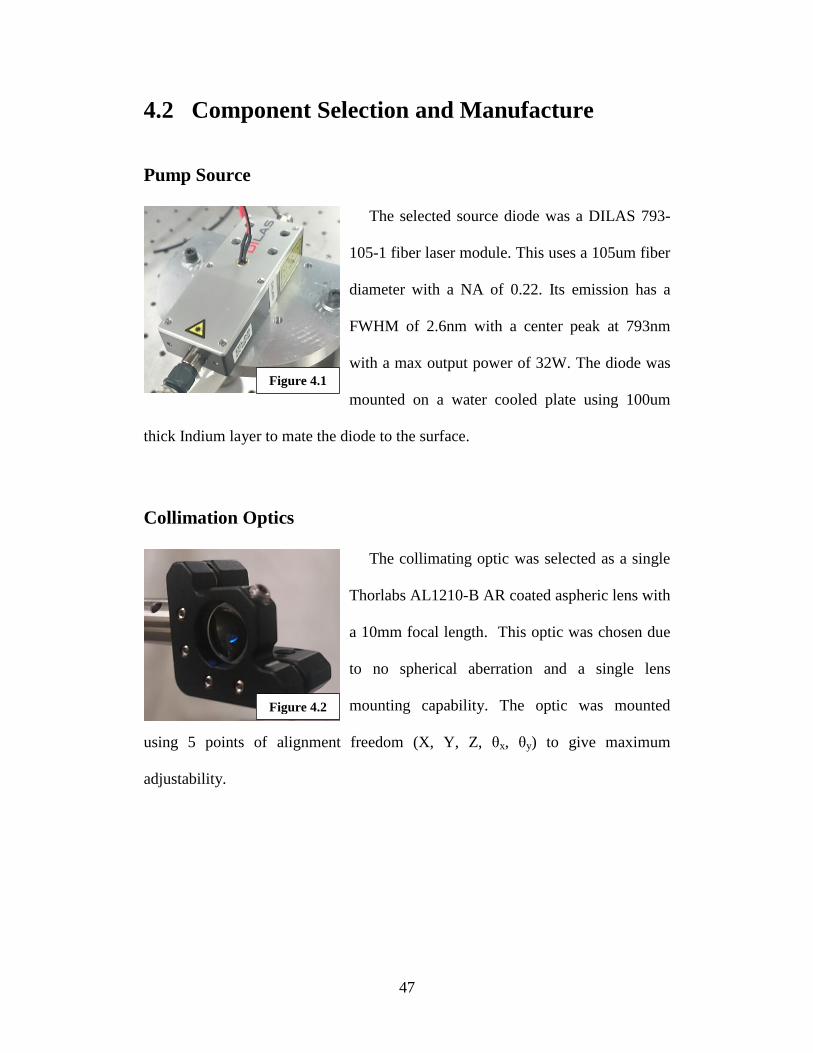
Pump Source
The selected source diode was a DILAS 793-
105-1 fiber laser module. This uses a 105um fiber
diameter with a NA of 0.22. Its emission has a
FWHM of 2.6nm with a center peak at 793nm
with a max output power of 32W. The diode was
mounted on a water cooled plate using 100um
thick Indium layer to mate the diode to the surface.
Collimation Optics
The collimating optic was selected as a single
Thorlabs AL1210-B AR coated aspheric lens with
a 10mm focal length. This optic was chosen due
to no spherical aberration and a single lens
mounting capability. The optic was mounted
using 5 points of alignment freedom (X, Y, Z, θx, θy) to give maximum
adjustability.
Figure 4.1
Figure 4.2

48
Parabolic Mirror
The focusing mirror was chosen to have a
focal length of 35mm with an external diameter
of 78mm and an internal hole aperture of 20mm.
It was manufactured as a parabola (-1 conic
constant) using an aluminum substrate with an
enhanced aluminum coating centered at 795nm,
giving approximately a 95.5% reflection at 793nm. This mirror was selected due
to its cheap cost and quick manufacturing time.
The parabolic mirror was mounted using a 5 point configuration with the radial
supports at 90o separation for minimum radial deflection, and with three back
supports equal spaced on a circle located at 0.707 of the radius for minimum axial
deflection [22]. The mirror was then mounted using 5 points of alignment
freedom (X, Y, Z, θx, θy) to give maximum adjustability.
Fold Mirrors
The four fold mirrors were selected using
modified Thorlabs BBSQ2-E03 2”x2” square
dielectric broadband coated mirrors (750-
1100nm). They have a reflectance of >99.5% at
45o angle of incidence. The mirrors were
modified using a diamond cutting wheel to cut
approximately a 1 inch angle off the corner of the mirror.
Figure 4.3
Figure 30
Figure 4.4
49
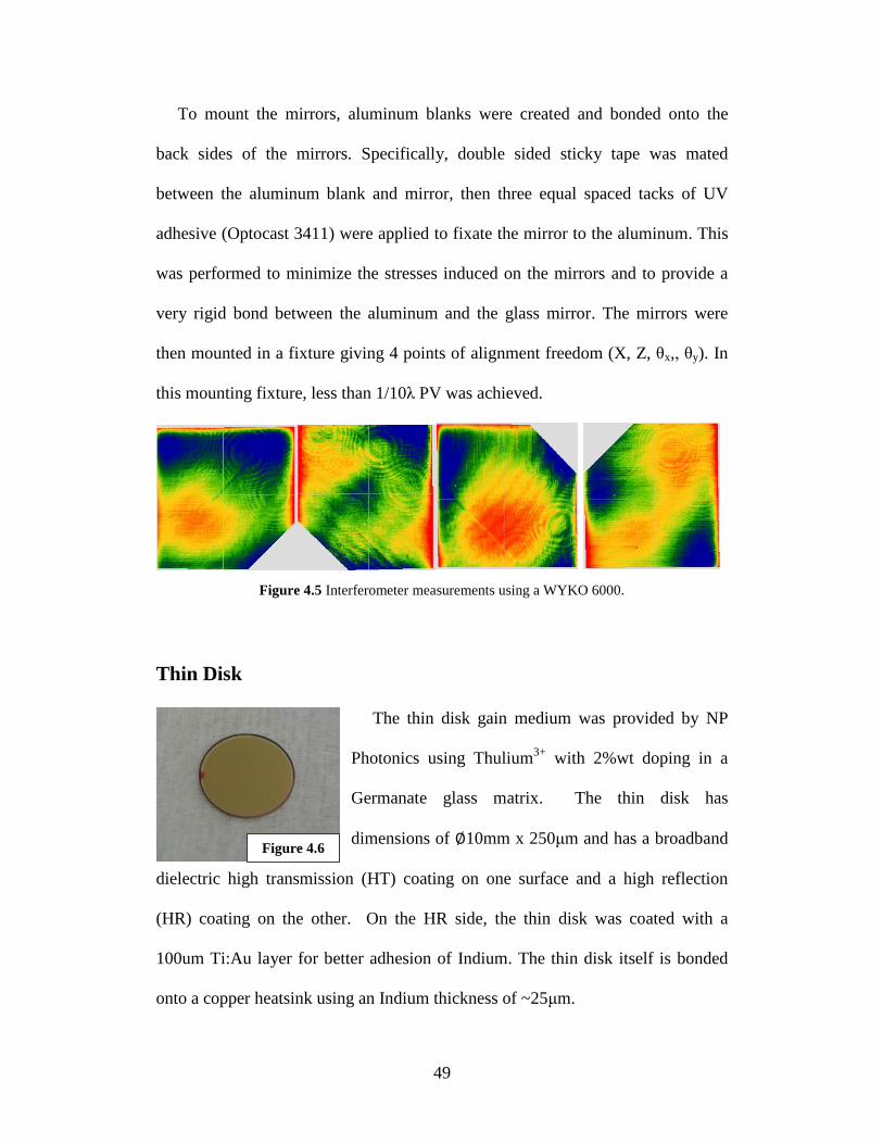
To mount the mirrors, aluminum blanks were created and bonded onto the
back sides of the mirrors. Specifically, double sided sticky tape was mated
between the aluminum blank and mirror, then three equal spaced tacks of UV
adhesive (Optocast 3411) were applied to fixate the mirror to the aluminum. This
was performed to minimize the stresses induced on the mirrors and to provide a
very rigid bond between the aluminum and the glass mirror. The mirrors were
then mounted in a fixture giving 4 points of alignment freedom (X, Z, θx,, θy). In
this mounting fixture, less than 1/10λ PV was achieved.
Figure 4.5 Interferometer measurements using a WYKO 6000.
Thin Disk
The thin disk gain medium was provided by NP
Photonics using Thulium3+
with 2%wt doping in a
Germanate glass matrix. The thin disk has
dimensions of ∅10mm x 250μm and has a broadband
dielectric high transmission (HT) coating on one surface and a high reflection
(HR) coating on the other. On the HR side, the thin disk was coated with a
100um Ti:Au layer for better adhesion of Indium. The thin disk itself is bonded
onto a copper heatsink using an Indium thickness of ~25μm.
Figure 4.6

50
Thin Disk Heatsink
The heatsink uses a custom machined 99.9%
copper mount with a wall thickness of ~1mm.
The copper face was polished to a surface flatness
about 0.95λ PV error. The copper heatsink was
coated with ~100nm Ti:Au to prevent oxidation
and to prevent Indium from diffusing into it [27].
The design uses a water inlet to flow against
the surface of the copper face where the thin disk
is mounted. The tube in the center can be
swapped out so water flowing into the thin disk
surface can be optimized.
The thin disk heatsink was mounted using 3
degrees of alignment freedom (Z, θx, θy). The
mechanical mounts were minimized to fit in the
small working space available. The thin disk in
the mount had less than a 1.1λ PV error.
Figure 4.7
Figure 4.8
Figure 4.9
Thin Disk
51
Resonator Configuration
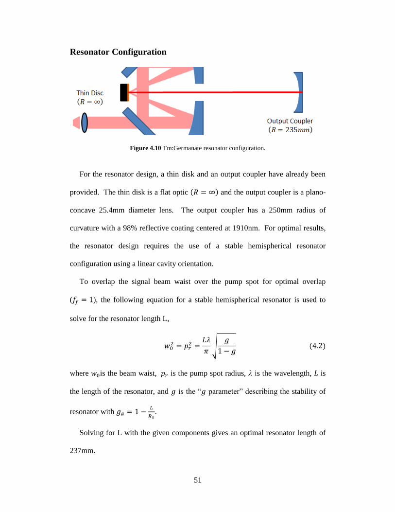
Figure 4.10 Tm:Germanate resonator configuration.
For the resonator design, a thin disk and an output coupler have already been
provided. The thin disk is a flat optic (𝑅 = ∞) and the output coupler is a plano-
concave 25.4mm diameter lens. The output coupler has a 250mm radius of
curvature with a 98% reflective coating centered at 1910nm. For optimal results,
the resonator design requires the use of a stable hemispherical resonator
configuration using a linear cavity orientation.
To overlap the signal beam waist over the pump spot for optimal overlap
(𝑓𝑓 = 1), the following equation for a stable hemispherical resonator is used to
solve for the resonator length L,
𝑤02 = 𝑝𝑟
2 =𝐿𝜆
𝜋√
𝑔
1 − 𝑔 (4.2)
where 𝑤0is the beam waist, 𝑝𝑟 is the pump spot radius, 𝜆 is the wavelength, 𝐿 is
the length of the resonator, and 𝑔 is the “𝑔 parameter” describing the stability of
resonator with 𝑔# = 1 −𝐿
𝑅#.
Solving for L with the given components gives an optimal resonator length of
237mm.

52
Final System Layout
The optical system is laid out on a 12”x12” breadboard so the pump chamber
can be transported for alignment and tested at different locations.
Figure 4.11 Solidworks model of pump module.
Figure 4.12 Solidworks model of pump optics.
53
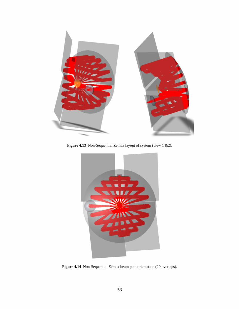
Figure 4.13 Non-Sequential Zemax layout of system (view 1 &2).
Figure 4.14 Non-Sequential Zemax beam path orientation (20 overlaps).
54
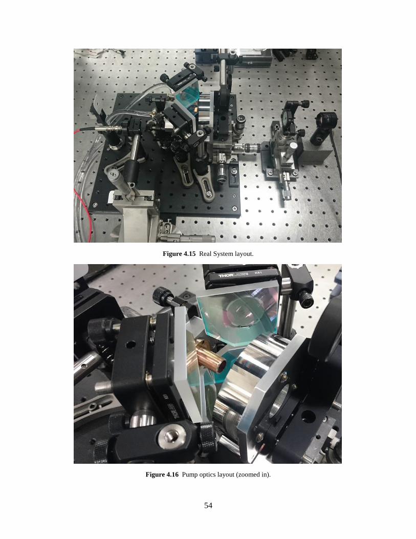
Figure 4.15 Real System layout.
Figure 4.16 Pump optics layout (zoomed in).

55
4.3 Alignment and Assembly
The top-level process used to align the thin disk laser is presented. Actual step-
by-step instructions for the pump chamber alignment are described in the
appendix B. The process can incorporate other creative techniques and various
devices/tools to ultimately achieve the same alignment goal. As a top level setup,
the following alignment steps occurs,
(i) Thin Disk Reference Mirror to Parabolic Mirror
(ii) Four Fold Mirrors
(iii) Pump Source and Collimation Optics
(iv) Thin Disk and Resonator Optics
Figure 4.17 Pump chamber alignment using an interferometer as a large diameter collimator.
56
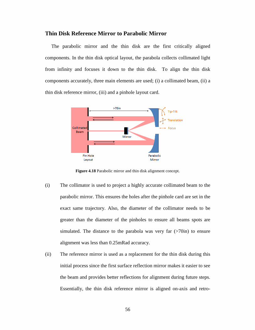
Thin Disk Reference Mirror to Parabolic Mirror
The parabolic mirror and the thin disk are the first critically aligned
components. In the thin disk optical layout, the parabola collects collimated light
from infinity and focuses it down to the thin disk. To align the thin disk
components accurately, three main elements are used; (i) a collimated beam, (ii) a
thin disk reference mirror, (iii) and a pinhole layout card.
Figure 4.18 Parabolic mirror and thin disk alignment concept.
(i) The collimator is used to project a highly accurate collimated beam to the
parabolic mirror. This ensures the holes after the pinhole card are set in the
exact same trajectory. Also, the diameter of the collimator needs to be
greater than the diameter of the pinholes to ensure all beams spots are
simulated. The distance to the parabola was very far (>70in) to ensure
alignment was less than 0.25mRad accuracy.
(ii) The reference mirror is used as a replacement for the thin disk during this
initial process since the first surface reflection mirror makes it easier to see
the beam and provides better reflections for alignment during future steps.
Essentially, the thin disk reference mirror is aligned on-axis and retro-
57
reflected to the collimator. The thin disk can also be used, but the beam
will be more difficult to see on the white retro-reflection pin-hole card.
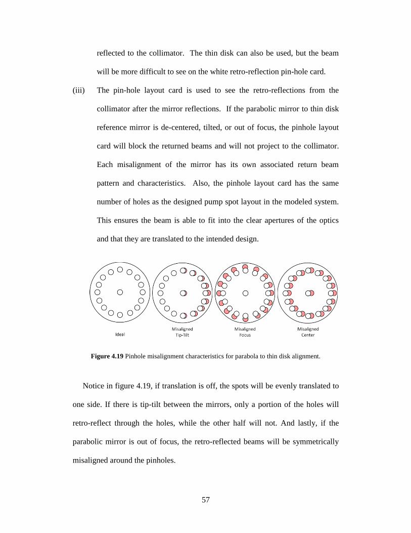
(iii) The pin-hole layout card is used to see the retro-reflections from the
collimator after the mirror reflections. If the parabolic mirror to thin disk
reference mirror is de-centered, tilted, or out of focus, the pinhole layout
card will block the returned beams and will not project to the collimator.
Each misalignment of the mirror has its own associated return beam
pattern and characteristics. Also, the pinhole layout card has the same
number of holes as the designed pump spot layout in the modeled system.
This ensures the beam is able to fit into the clear apertures of the optics
and that they are translated to the intended design.
Figure 4.19 Pinhole misalignment characteristics for parabola to thin disk alignment.
Notice in figure 4.19, if translation is off, the spots will be evenly translated to
one side. If there is tip-tilt between the mirrors, only a portion of the holes will
retro-reflect through the holes, while the other half will not. And lastly, if the
parabolic mirror is out of focus, the retro-reflected beams will be symmetrically
misaligned around the pinholes.

58
Four Fold Mirrors
The four fold mirrors are the most critically aligned components in the entire
setup. The mirror angles are dependent on the number of times the pump passes
through the gain medium decided in the design. For this design, 20 passes of the
thin disk was selected for two specific reasons; mechanical limitations of the
mirror dimension to fit between two beams, and the clear aperture of the mirror’s
coating.
Only two critical components are needed to align the four fold mirrors; the
auto-collimator, and a pin-hole layout card. Also, the parabolic mirror must be
removed temporarily so the full layout of the beams can project to the four fold
mirrors, and the setup must be spun around so the thin disk reference mirror faces
the collimator. Removal of the parabolic mirror is supplemented by placing
mechanical reference mounts so the parabola can be placed back into the system
later with good enough accuracy.
Figure 4.20 Thin disks four fold mirrors alignment concept.

59
The four fold mirrors are aligned to the auto-collimator by aligning the beams
to pass through the pinhole card. The emphasis is to precisely position the
necessary angles on the fold mirrors so that the beams coming in on-axis will
leave on-axis in the correct locations. One of the pinhole beams that reflects off
the thin disk alignment mirror needs to be centered in the same location as where
the parabola focused its spots. This ensures the beam profile matches the parabola
locations.
Figure 4.21 Angle adjustment of four fold mirrors.
In this setup, the bottom mirror angles are re-iteratively adjusted so that the
beams go to the holes down or up from the opposite holes, depending on direction
of travel (see figure 4.21, left). The top mirrors orient the beams symmetrically
opposite of each other (figure 4.21, right). Mirrors are adjusted such that the left
mirror needs to be adjusted to have the right beams go through the right holes, and
the right mirror needs to be adjusted to have the left beam go through the left
holes. This was re-iterated until all holes line up.
60
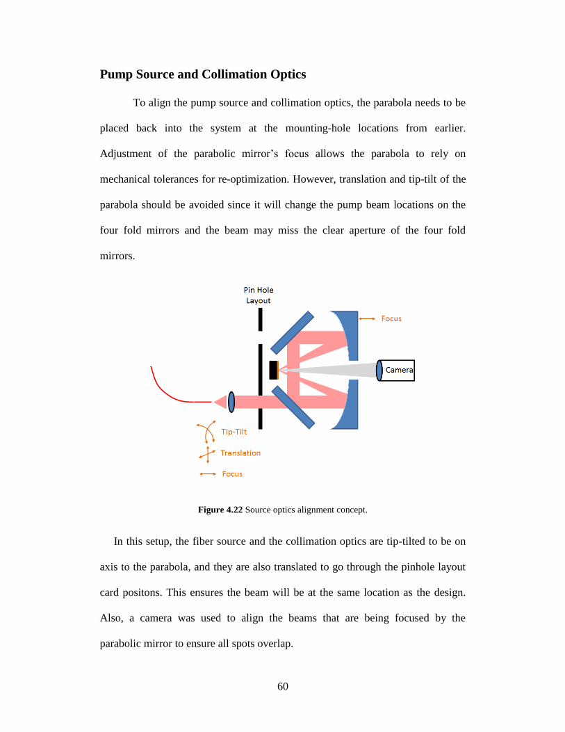
Pump Source and Collimation Optics
To align the pump source and collimation optics, the parabola needs to be
placed back into the system at the mounting-hole locations from earlier.
Adjustment of the parabolic mirror’s focus allows the parabola to rely on
mechanical tolerances for re-optimization. However, translation and tip-tilt of the
parabola should be avoided since it will change the pump beam locations on the
four fold mirrors and the beam may miss the clear aperture of the four fold
mirrors.
Figure 4.22 Source optics alignment concept.
In this setup, the fiber source and the collimation optics are tip-tilted to be on
axis to the parabola, and they are also translated to go through the pinhole layout
card positons. This ensures the beam will be at the same location as the design.
Also, a camera was used to align the beams that are being focused by the
parabolic mirror to ensure all spots overlap.

61
Figure 4.23 Prototype of source optics and pump chamber.
Ideal Parabola Focus In Parabola Focus Out
Collimation Angle Left Collimation Angle Right
Figure 4.24 Source optics beam alignment characteristics.
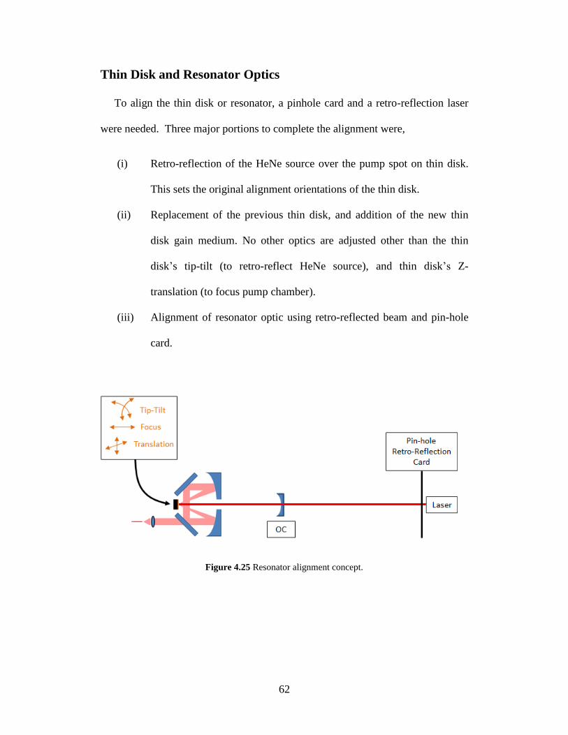
62
Thin Disk and Resonator Optics
To align the thin disk or resonator, a pinhole card and a retro-reflection laser
were needed. Three major portions to complete the alignment were,
(i) Retro-reflection of the HeNe source over the pump spot on thin disk.
This sets the original alignment orientations of the thin disk.
(ii) Replacement of the previous thin disk, and addition of the new thin
disk gain medium. No other optics are adjusted other than the thin
disk’s tip-tilt (to retro-reflect HeNe source), and thin disk’s Z-
translation (to focus pump chamber).
(iii) Alignment of resonator optic using retro-reflected beam and pin-hole
card.
Figure 4.25 Resonator alignment concept.

63
Chapter 5
System Performance
To gain insight into the expected performance of the designed thin disk laser,
several predictive models have been developed. The first model to understand is
the pump chamber’s optical performance and capabilities. The next presented
model is the predicted power output with the selected components using the
equations derived in chapter 3. Lastly, the experimental results of the system are
presented and explained.
5.1 Pump Spot Analysis
To model the source and pump chamber, Non-Sequential ZEMAX was used.
This gave detailed data on the beam characteristics and performance. The
collected data from the input power was normalized to 1 Watt to give insight into
intensity variations. Resonator pulse propagation and beam quality have not been
analyzed in this thesis since we are only concerned with the power output.

64
Fiber Source
The pump source was first characterized and modelled to accurately analyze
the final pump spot onto the thin disk. Capturing the beam profile consisted of
measuring the output of the DILAS 793nm fiber diode by scanning across
horizontally with a power meter using a small pinhole aperture. The data was
then compiled, normalized, and divided into 10 segments. This data was then
entered into ZEMAX; specifically, the source was modelled using a ‘Radial
Source’ object type with the data from the 10 segments calculated earlier, as well
as the fiber emission angle calculated from the NA given from the DILAS fiber
datasheet.
Figure 5.1 Zemax modelled data from a DILAS 793nm fiber diode.
As can be seen in the horizontal profile, the beam width after the collimating
lens (at the 1
𝑒2 radial location point), compares very close to the first order
calculated value of 4.51mm. This should give a good indication how the pump
spot looks like in the thin disk.
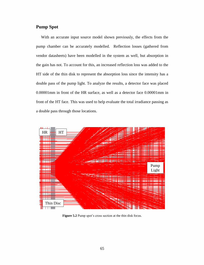
65
Pump Spot
With an accurate input source model shown previously, the effects from the
pump chamber can be accurately modelled. Reflection losses (gathered from
vendor datasheets) have been modelled in the system as well, but absorption in
the gain has not. To account for this, an increased reflection loss was added to the
HT side of the thin disk to represent the absorption loss since the intensity has a
double pass of the pump light. To analyze the results, a detector face was placed
0.00001mm in front of the HR surface, as well as a detector face 0.00001mm in
front of the HT face. This was used to help evaluate the total irradiance passing as
a double pass through those locations.
Figure 5.2 Pump spot’s cross section at the thin disk focus.
HR HT
Thin Disc
Pump
Light
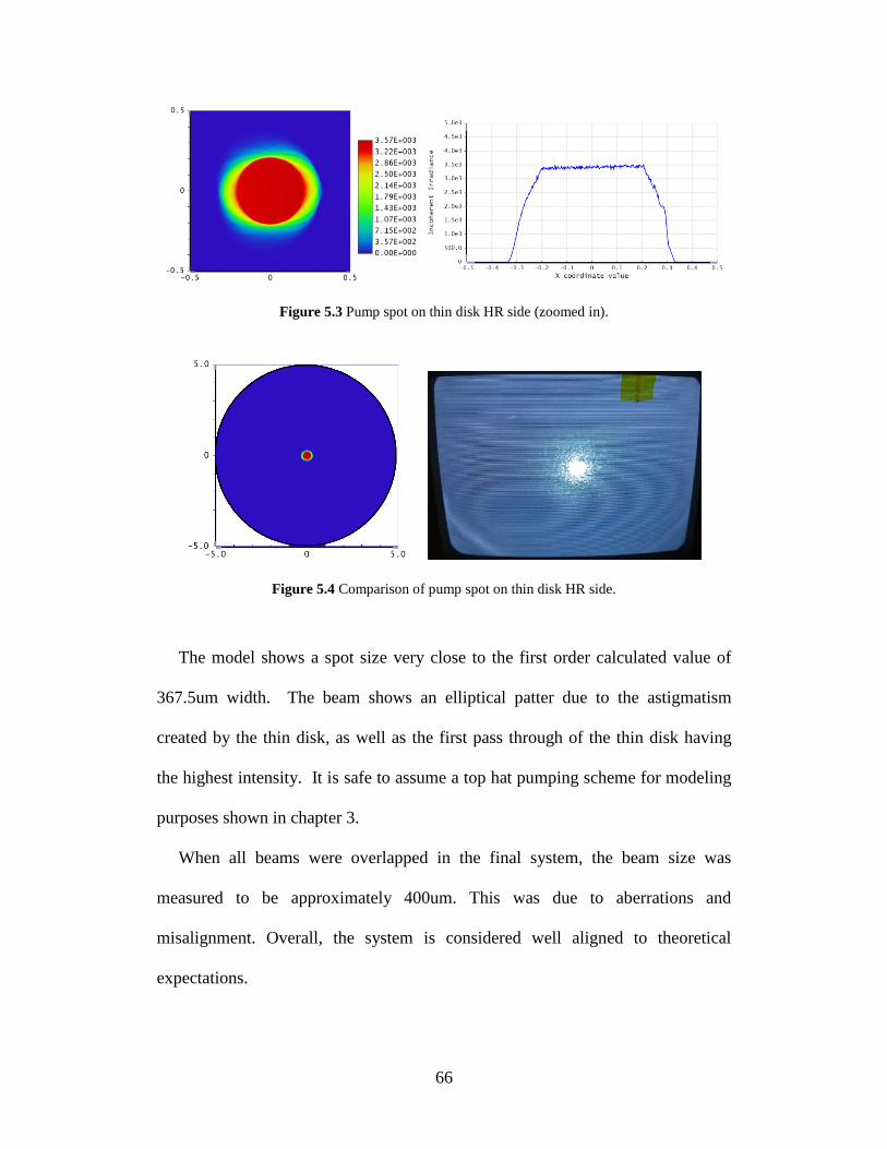
66
Figure 5.3 Pump spot on thin disk HR side (zoomed in).
Figure 5.4 Comparison of pump spot on thin disk HR side.
The model shows a spot size very close to the first order calculated value of
367.5um width. The beam shows an elliptical patter due to the astigmatism
created by the thin disk, as well as the first pass through of the thin disk having
the highest intensity. It is safe to assume a top hat pumping scheme for modeling
purposes shown in chapter 3.
When all beams were overlapped in the final system, the beam size was
measured to be approximately 400um. This was due to aberrations and
misalignment. Overall, the system is considered well aligned to theoretical
expectations.

67
Tm:Germanate Output Power Model
Using the model derived in chapter 3, the output power is calculated for the
components selected in chapter 4. The table below shows the constants used for
the model.
Parameter Symbol Value
Signal Wavelength λs 1910 nm
Pump Wavelength λp 793 nm
Losses in Medium l 0
Thickness of Thin Disk L 250 μm
Diameter of Pump Spot Dp 367.5 μm
Total Population Density Nt 5.2x1026
m-3
Radiative Lifetime t21 2.5x10⁻³
sec
HR Thin Disk Reflectance ROC 99.5%
Output Coupler Reflectance RHR 98%
Parabolic Reflectance P 95.5%
Fold Mirror Reflectance F 99.5%
Number of Pump Beam Passes N 20
Pump Absorption Cross Section 𝜎𝑝𝑎 4.472800x10
-25 m
2
Pump Emission Cross Section 𝜎𝑝𝑒 1x10
-100 m
2 (No Info)
Signal Absorption Cross Section 𝜎𝑠𝑎 0.129504x10
-25 m
2
Signal Emission Cross Section 𝜎𝑠𝑎 1.8114100x10
-25 m
2
Radius of Thin Disk 𝑟𝐻𝑅 ∞ (Flat)
Radius of Output Coupler 𝑟𝑂𝐶 250 mm
Length of the Resonator 𝐿𝑟𝑒𝑠 237 mm
Signal-Power Coupling Efficiency 𝜅𝑠𝑝 ~.99* (Varying)
Table 5.1 Tm:Germanate model parameters.
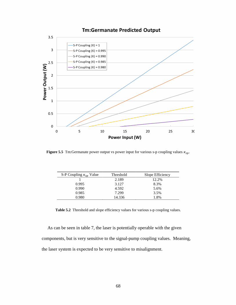
68
Figure 5.5 Tm:Germanate power output vs power input for various s-p coupling values 𝜅𝑠𝑝.
S-P Coupling 𝜅𝑠𝑝 Value Threshold Slope Efficiency
1 2.189 12.2%
0.995 3.127 8.3%
0.990 4.592 5.6%
0.985 7.299 3.5%
0.980 14.336 1.8%
Table 5.2 Threshold and slope efficiency values for various s-p coupling values.
As can be seen in table 7, the laser is potentially operable with the given
components, but is very sensitive to the signal-pump coupling values. Meaning,
the laser system is expected to be very sensitive to misalignment.
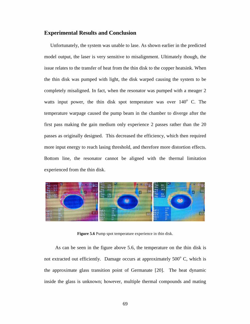
69
Experimental Results and Conclusion
Unfortunately, the system was unable to lase. As shown earlier in the predicted
model output, the laser is very sensitive to misalignment. Ultimately though, the
issue relates to the transfer of heat from the thin disk to the copper heatsink. When
the thin disk was pumped with light, the disk warped causing the system to be
completely misaligned. In fact, when the resonator was pumped with a meager 2
watts input power, the thin disk spot temperature was over 140o C. The
temperature warpage caused the pump beam in the chamber to diverge after the
first pass making the gain medium only experience 2 passes rather than the 20
passes as originally designed. This decreased the efficiency, which then required
more input energy to reach lasing threshold, and therefore more distortion effects.
Bottom line, the resonator cannot be aligned with the thermal limitation
experienced from the thin disk.
Figure 5.6 Pump spot temperature experience in thin disk.
As can be seen in the figure above 5.6, the temperature on the thin disk is
not extracted out efficiently. Damage occurs at approximately 500o C, which is
the approximate glass transition point of Germanate [20]. The heat dynamic
inside the glass is unknown; however, multiple thermal compounds and mating
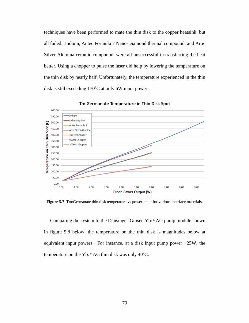
70
techniques have been performed to mate the thin disk to the copper heatsink, but
all failed. Indium, Antec Formula 7 Nano-Diamond thermal compound, and Artic
Silver Alumina ceramic compound, were all unsuccessful in transferring the heat
better. Using a chopper to pulse the laser did help by lowering the temperature on
the thin disk by nearly half. Unfortunately, the temperature experienced in the thin
disk is still exceeding 170oC at only 6W input power.
Figure 5.7 Tm:Germanate thin disk temperature vs power input for various interface materials.
Comparing the system to the Dausinger-Guisen Yb:YAG pump module shown
in figure 5.8 below, the temperature on the thin disk is magnitudes below at
equivalent input powers. For instance, at a disk input pump power ~25W, the
temperature on the Yb:YAG thin disk was only 40oC.

71
Figure 5.8 Pump spot temperature in Yb:YAG thin disk laser.
In conclusion, the Tm:Germanate laser will not lase unless the thin disk’s heat
is extracted out. Even though the thin disk will not lase, detailed design
instructions, models, and alignment processes have been developed so other gain
materials and enhancements to the thin disk can be experimented with.
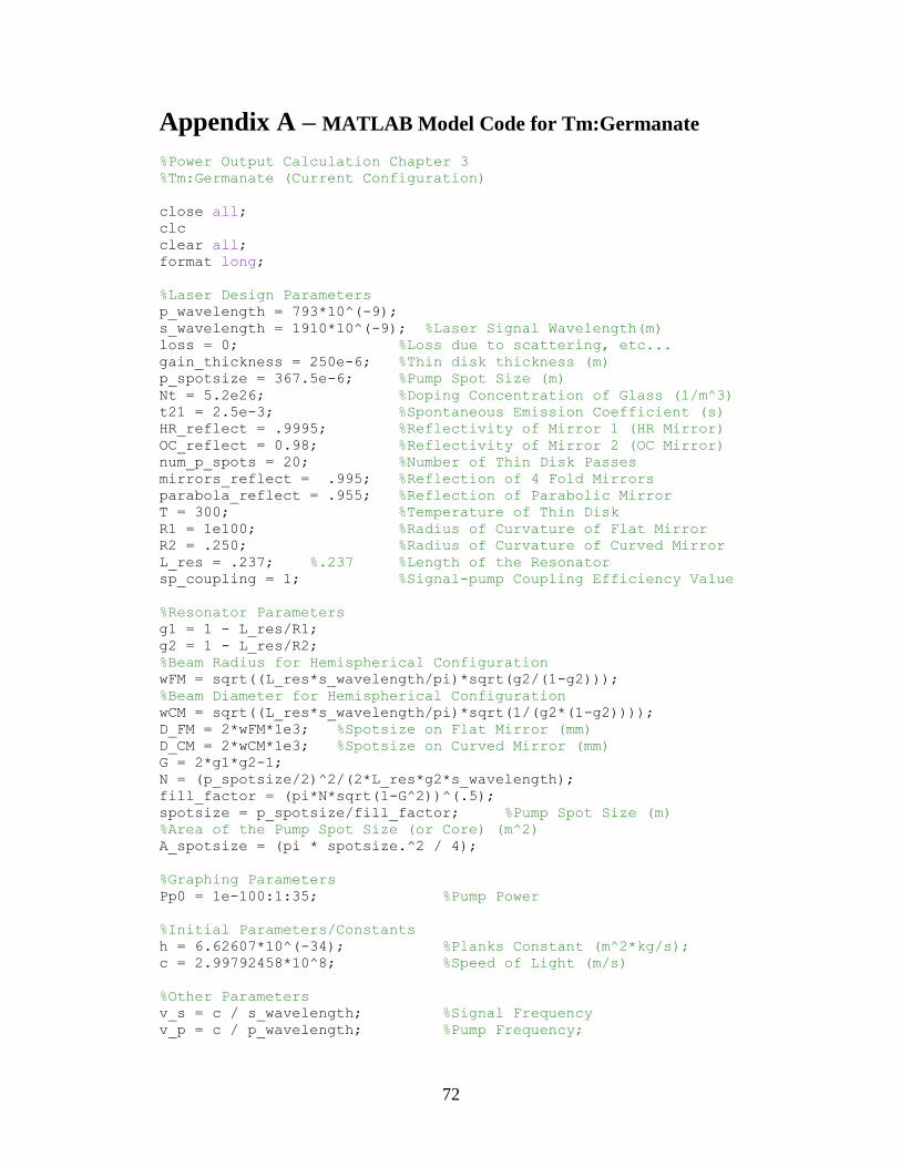
72
Appendix A – MATLAB Model Code for Tm:Germanate
%Power Output Calculation Chapter 3
%Tm:Germanate (Current Configuration)
close all;
clc
clear all;
format long;
%Laser Design Parameters
p_wavelength = 793*10^(-9);
s_wavelength = 1910*10^(-9); %Laser Signal Wavelength(m)
loss = 0; %Loss due to scattering, etc...
gain_thickness = 250e-6; %Thin disk thickness (m)
p_spotsize = 367.5e-6; %Pump Spot Size (m)
Nt = 5.2e26; %Doping Concentration of Glass (1/m^3)
t21 = 2.5e-3; %Spontaneous Emission Coefficient (s)
HR_reflect = .9995; %Reflectivity of Mirror 1 (HR Mirror)
OC_reflect = 0.98; %Reflectivity of Mirror 2 (OC Mirror)
num_p_spots = 20; %Number of Thin Disk Passes
mirrors_reflect = .995; %Reflection of 4 Fold Mirrors
parabola_reflect = .955; %Reflection of Parabolic Mirror
T = 300; %Temperature of Thin Disk
R1 = 1e100; %Radius of Curvature of Flat Mirror
R2 = .250; %Radius of Curvature of Curved Mirror
L_res = .237; %.237 %Length of the Resonator
sp_coupling = 1; %Signal-pump Coupling Efficiency Value
%Resonator Parameters
g1 = 1 - L_res/R1;
g2 = 1 - L_res/R2;
%Beam Radius for Hemispherical Configuration
wFM = sqrt((L_res*s_wavelength/pi)*sqrt(g2/(1-g2)));
%Beam Diameter for Hemispherical Configuration
wCM = sqrt((L_res*s_wavelength/pi)*sqrt(1/(g2*(1-g2))));
D_FM = 2*wFM*1e3; %Spotsize on Flat Mirror (mm)
D_CM = 2*wCM*1e3; %Spotsize on Curved Mirror (mm)
G = 2*g1*g2-1;
N = (p_spotsize/2)^2/(2*L_res*g2*s_wavelength);
fill_factor = (pi*N*sqrt(1-G^2))^(.5);
spotsize = p_spotsize/fill_factor; %Pump Spot Size (m)
%Area of the Pump Spot Size (or Core) (m^2)
A_spotsize = (pi * spotsize.^2 / 4);
%Graphing Parameters
Pp0 = 1e-100:1:35; %Pump Power
%Initial Parameters/Constants
h = 6.62607*10^(-34); %Planks Constant (m^2*kg/s);
c = 2.99792458*10^8; %Speed of Light (m/s)
%Other Parameters
v_s = c / s_wavelength; %Signal Frequency
v_p = c / p_wavelength; %Pump Frequency;
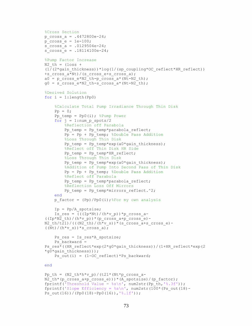
73
%Cross Section
p_cross_a = .4472800e-24;
p_cross_e = 1e-100;
s_cross_a = .0129504e-24;
s_cross_e = .18114100e-24;
%Pump Factor Increase
N2_th = (loss +
(1/(2*gain_thickness))*log(1/(sp_coupling*OC_reflect*HR_reflect))
+s_cross_a*Nt)/(s_cross_e+s_cross_a);
a0 = p_cross_e*N2_th-p_cross_a*(Nt-N2_th);
g0 = s_cross_e*N2_th-s_cross_a*(Nt-N2_th);
%Derived Solution
for i = 1:length(Pp0)
%Calculate Total Pump Irradiance Through Thin Disk
Pp = 0;
Pp_temp = Pp0(i); %Pump Power
for j = 1:num_p_spots/2
%Reflection off Parabola
Pp_temp = Pp_temp*parabola_reflect;
Pp = Pp + Pp_temp; %Double Pass Addition
%Loss Through Thin Disk
Pp_temp = Pp_temp*exp(a0*gain_thickness);
%Reflect off Thin Disk HR Side
Pp_temp = Pp_temp*HR_reflect;
%Loss Through Thin Disk
Pp_temp = Pp_temp*exp(a0*gain_thickness);
%Addition of Pump Into Second Pass of Thin Disk
Pp = Pp + Pp_temp; %Double Pass Addition
%Reflect off Parabola
Pp_temp = Pp_temp*parabola_reflect;
%Reflection Loss Off Mirrors
Pp_temp = Pp_temp*mirrors_reflect.^2;
end
p_factor = (Pp)/Pp0(i);%For my own analysis
Ip = Pp/A_spotsize;
Is_res = (((Ip*Nt)/(h*v_p))*p_cross_a-
((Ip*N2_th)/(h*v_p))*(p_cross_a+p_cross_e)-
N2_th/t21)/(((N2_th)/(h*v_s))*(s_cross_a+s_cross_e)-
((Nt)/(h*v_s))*s_cross_a);
Ps_res = Is_res*A_spotsize;
Ps_backward =
Ps_res*((HR_reflect*exp(2*g0*gain_thickness))/(1+HR_reflect*exp(2
*g0*gain_thickness)));
Ps_out(i) = (1-OC_reflect)*Ps_backward;
end
Pp_th = (N2_th*h*v_p)/(t21*(Nt*p_cross_a-
N2_th*(p_cross_a+p_cross_e)))*(A_spotsize)/(p_factor);
fprintf('Threshold Value = %s\n', num2str(Pp_th,'%.3f'));
fprintf('Slope Efficiency = %s\n', num2str(100*(Ps_out(18)-
Ps_out(16))/(Pp0(18)-Pp0(16)),'%.1f'));

74
figure;
plot(Pp0, Ps_out);
title('Laser Out vs Fiber Input'); xlabel('Fiber Input Power
(W)'); ylabel('Is Out (W)');
%axis([0, length(Ip0), 0, 60]);
%Save File
final_result=[Pp0',Ps_out'];
save 'TDL_MyDerived_Model_Tm-Germanate.txt' final_result -ASCII;

75
Appendix B – ZEMAX Pump Design Procedure
1. Determine the number of passes through the thin disk and calculate the
cross angle distances.
2. Load Non-Sequential Zemax and set the wavelength and parameters.
3. Add in 8 surfaces and make them symmetrically placed around a surface
at the desired radial distances with diameters equal to the beam spot size
calculated by first order parameters.
Make them 40% transparent.
Select ‘Always’ for the option ‘Rays Ignore Object’.
4. Add in a parabolic mirror and a flat mirror as a ‘standard surface’.
Place the flat mirror at the location where thin disk focus point.
Make them 40% Transparent.
5. Insert a “Source Ray” and project the ray at the radial distance desired into
the parabola.
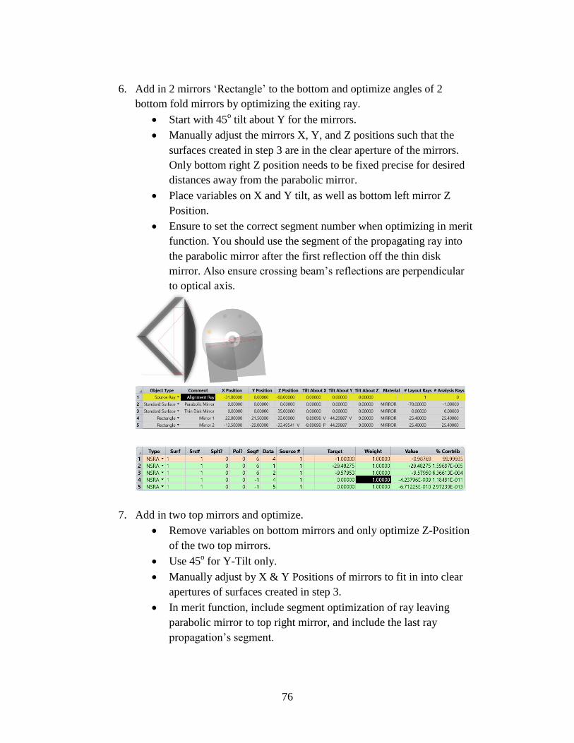
76
6. Add in 2 mirrors ‘Rectangle’ to the bottom and optimize angles of 2
bottom fold mirrors by optimizing the exiting ray.
Start with 45o tilt about Y for the mirrors.
Manually adjust the mirrors X, Y, and Z positions such that the
surfaces created in step 3 are in the clear aperture of the mirrors.
Only bottom right Z position needs to be fixed precise for desired
distances away from the parabolic mirror.
Place variables on X and Y tilt, as well as bottom left mirror Z
Position.
Ensure to set the correct segment number when optimizing in merit
function. You should use the segment of the propagating ray into
the parabolic mirror after the first reflection off the thin disk
mirror. Also ensure crossing beam’s reflections are perpendicular
to optical axis.
7. Add in two top mirrors and optimize.
Remove variables on bottom mirrors and only optimize Z-Position
of the two top mirrors.
Use 45o for Y-Tilt only.
Manually adjust by X & Y Positions of mirrors to fit in into clear
apertures of surfaces created in step 3.
In merit function, include segment optimization of ray leaving
parabolic mirror to top right mirror, and include the last ray
propagation’s segment.
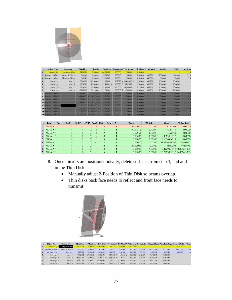
77
8. Once mirrors are positioned ideally, delete surfaces from step 3, and add
in the Thin Disk.
Manually adjust Z Position of Thin Disk so beams overlap.
Thin disks back face needs to reflect and front face needs to
transmit.

78
9. Use default merit function to optimize Z position of thin disk.
Add a detector face to be 0.00001mm in front of the HR side of the
thin disk.
10. Add in source type into setup, and add in source collimation lens.
Use sequential analysis to determine optimal placement of
collimation lens in relation to the source. Set the system up to be
double telecentric with the parabolic mirror focal length the same
as the designed system.
11. Use default merit function again to optimize Z position of Thin Disk.
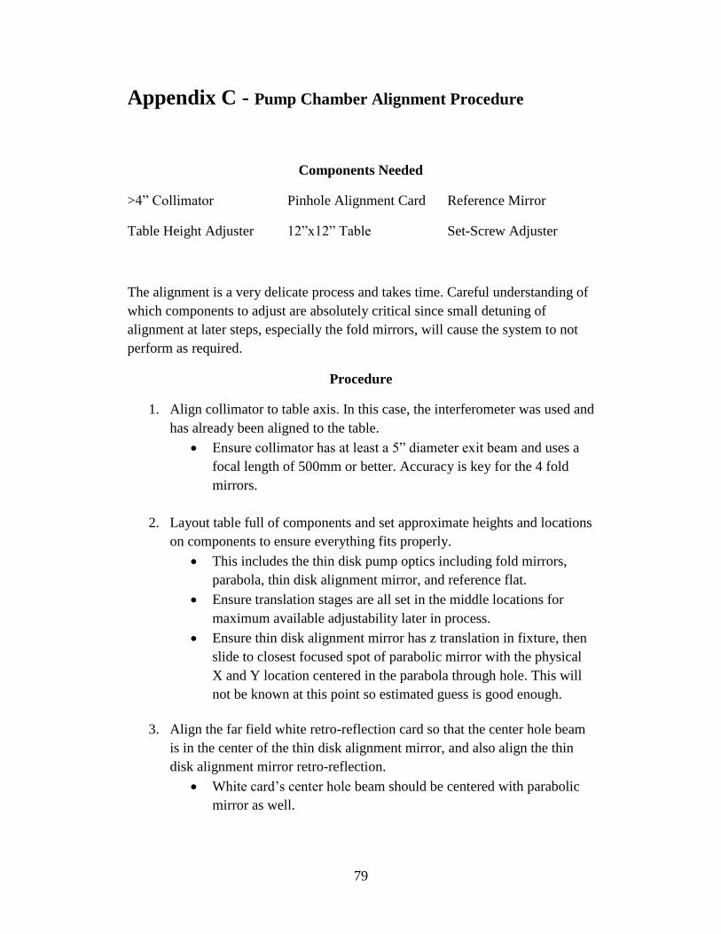
79
Appendix C - Pump Chamber Alignment Procedure
Components Needed
>4” Collimator Pinhole Alignment Card Reference Mirror
Table Height Adjuster 12”x12” Table Set-Screw Adjuster
The alignment is a very delicate process and takes time. Careful understanding of
which components to adjust are absolutely critical since small detuning of
alignment at later steps, especially the fold mirrors, will cause the system to not
perform as required.
Procedure
1. Align collimator to table axis. In this case, the interferometer was used and
has already been aligned to the table.
Ensure collimator has at least a 5” diameter exit beam and uses a
focal length of 500mm or better. Accuracy is key for the 4 fold
mirrors.
2. Layout table full of components and set approximate heights and locations
on components to ensure everything fits properly.
This includes the thin disk pump optics including fold mirrors,
parabola, thin disk alignment mirror, and reference flat.
Ensure translation stages are all set in the middle locations for
maximum available adjustability later in process.
Ensure thin disk alignment mirror has z translation in fixture, then
slide to closest focused spot of parabolic mirror with the physical
X and Y location centered in the parabola through hole. This will
not be known at this point so estimated guess is good enough.
3. Align the far field white retro-reflection card so that the center hole beam
is in the center of the thin disk alignment mirror, and also align the thin
disk alignment mirror retro-reflection.
White card’s center hole beam should be centered with parabolic
mirror as well.
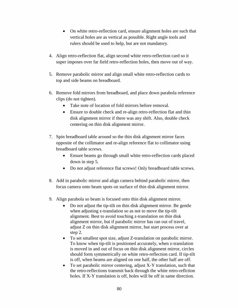
80
On white retro-reflection card, ensure alignment holes are such that
vertical holes are as vertical as possible. Right angle tools and
rulers should be used to help, but are not mandatory.
4. Align retro-reflection flat, align second white retro-reflection card so it
super imposes over far field retro-reflection holes, then move out of way.
5. Remove parabolic mirror and align small white retro-reflection cards to
top and side beams on breadboard.
6. Remove fold mirrors from breadboard, and place down parabola reference
clips (do not tighten).
Take note of location of fold mirrors before removal.
Ensure to double check and re-align retro-reflection flat and thin
disk alignment mirror if there was any shift. Also, double check
centering on thin disk alignment mirror.
7. Spin breadboard table around so the thin disk alignment mirror faces
opposite of the collimator and re-align reference flat to collimator using
breadboard table screws.
Ensure beams go through small white retro-reflection cards placed
down in step 5.
Do not adjust reference flat screws! Only breadboard table screws.
8. Add in parabolic mirror and align camera behind parabolic mirror, then
focus camera onto beam spots on surface of thin disk alignment mirror.
9. Align parabola so beam is focused onto thin disk alignment mirror.
Do not adjust the tip-tilt on thin disk alignment mirror. Be gentle
when adjusting z-translation so as not to move the tip-tilt
alignment. Best to avoid touching z-translation on thin disk
alignment mirror, but if parabolic mirror has ran out of travel,
adjust Z on thin disk alignment mirror, but start process over at
step 2.
To set smallest spot size, adjust Z-translation on parabolic mirror.
To know when tip-tilt is positioned accurately, when z-translation
is moved in and out of focus on thin disk alignment mirror, circles
should form symmetrically on white retro-reflection card. If tip-tilt
is off, when beams are aligned on one half, the other half are off.
To set parabolic mirror centering, adjust X-Y translation, such that
the retro-reflections transmit back through the white retro-reflction
holes. If X-Y translation is off, holes will be off in same direction.
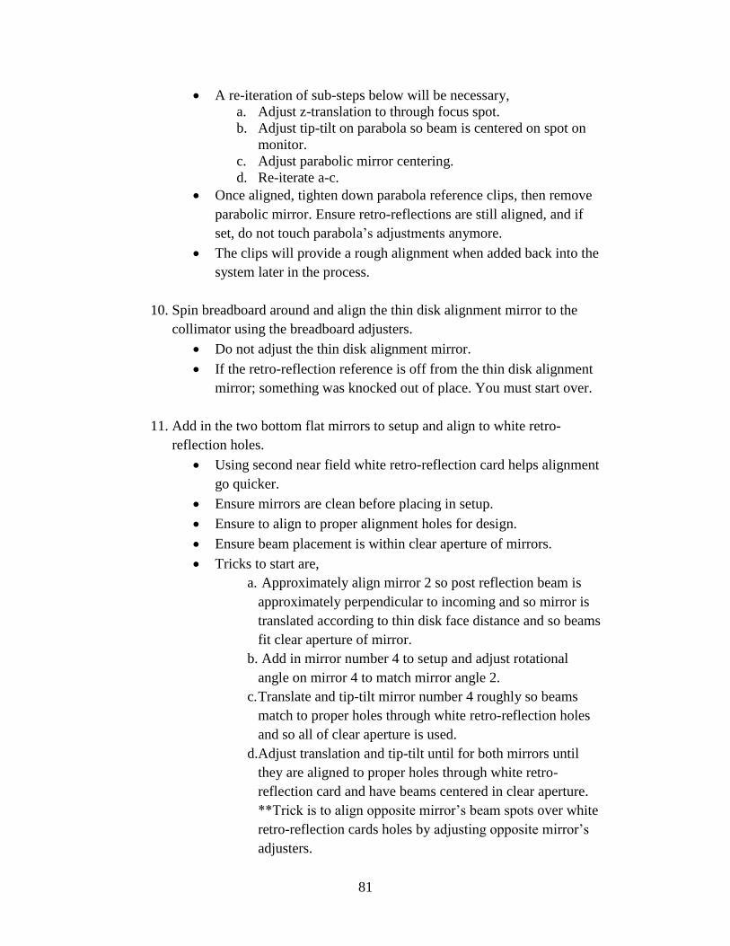
81
A re-iteration of sub-steps below will be necessary,
a. Adjust z-translation to through focus spot.
b. Adjust tip-tilt on parabola so beam is centered on spot on
monitor.
c. Adjust parabolic mirror centering.
d. Re-iterate a-c.
Once aligned, tighten down parabola reference clips, then remove
parabolic mirror. Ensure retro-reflections are still aligned, and if
set, do not touch parabola’s adjustments anymore.
The clips will provide a rough alignment when added back into the
system later in the process.
10. Spin breadboard around and align the thin disk alignment mirror to the
collimator using the breadboard adjusters.
Do not adjust the thin disk alignment mirror.
If the retro-reflection reference is off from the thin disk alignment
mirror; something was knocked out of place. You must start over.
11. Add in the two bottom flat mirrors to setup and align to white retro-
reflection holes.
Using second near field white retro-reflection card helps alignment
go quicker.
Ensure mirrors are clean before placing in setup.
Ensure to align to proper alignment holes for design.
Ensure beam placement is within clear aperture of mirrors.
Tricks to start are,
a. Approximately align mirror 2 so post reflection beam is
approximately perpendicular to incoming and so mirror is
translated according to thin disk face distance and so beams
fit clear aperture of mirror.
b. Add in mirror number 4 to setup and adjust rotational
angle on mirror 4 to match mirror angle 2.
c. Translate and tip-tilt mirror number 4 roughly so beams
match to proper holes through white retro-reflection holes
and so all of clear aperture is used.
d.Adjust translation and tip-tilt until for both mirrors until
they are aligned to proper holes through white retro-
reflection card and have beams centered in clear aperture.
**Trick is to align opposite mirror’s beam spots over white
retro-reflection cards holes by adjusting opposite mirror’s
adjusters.
82
e. Repeat d until all are aligned.
12. Place parabola on breadboard and ensure there is enough clearance for
optics. Remove when complete.
13. Add in two top flat mirrors to setup and align near field and to collimator
Essentially same as step 12.
14. Double check alignment on all optics by re-aligning the thin disk
alignment mirror using the breadboard adjuster screws.
They should all still be aligned. Minor changes may have occurred
due to weight added onto breadboard.
Do not adjust thin disk alignment mirror tip-tilt.
15. Add in fiber mount and center with entrance beam from white retro-
reflector card.
16. Add in parabolic mirror.
Be extremely careful.
Do not touch the translation or tip-tilt adjustments on the parabolic
mirror.
17. Once placed in and all screws tightened down, move setup so collimation
optics can be aligned.
At this point, various the fold mirrors and parabola must not be
changed. Doing so will through the system out of alignment and
make it very difficult to retain original characteristics.
Thin disk alignment mirror can be removed and replaced with thin
disk setup, but not before collimation optics are aligned.
18. Set previously aligned thin disk down onto table in new location and focus
a camera onto the surface of the thin disk reference mirror.
19. Add in fiber into the fiber mount and translate/angle beam so it is coming
in on axis to parabola and is translated through small white alignment
card.
20. Add in collimating optic and set focus. Collimated beam should go
through center hole of small white reflection card.
Set tip/tilt of collimating optics so back reflection is close to
source.

83
Translate X&Y on collimating optic to set beam convergence.
Also, set Z translation on parabola so all spots converge together.
21. Double check that all folding beams are in the clear apertures of the fold
mirrors. Check that all spots are indeed overlapping.
22. Align HeNe over pump spot and so beam is retro-reflected back to source.
23. Remove reference alignment thin disk and add in actual thin disk and
heatsink.
Do not adjust parabola or collimation optics.
Adjust tip-tilt on thin disk so HeNe is retro-reflected.
Adjust only thin disk Z-axis to set focus. Note; beams will not look
round. That’s ok.
24. Double check spots on fold mirrors again and ensure all spots overlap on
thin disk.
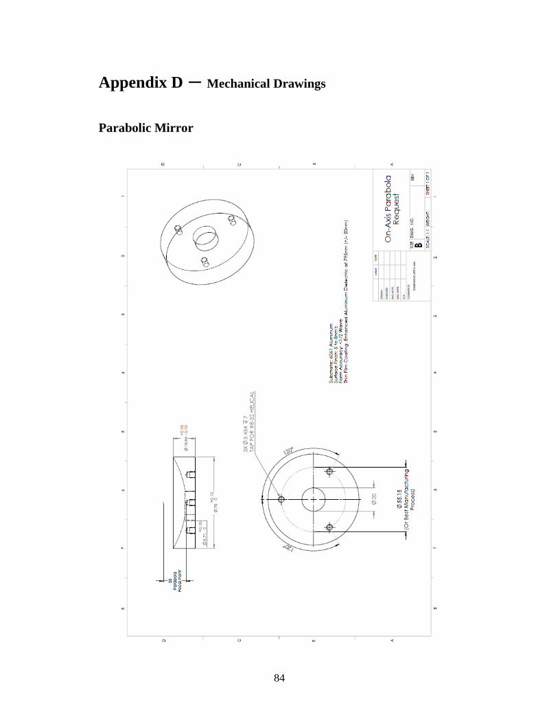
84
Appendix D – Mechanical Drawings
Parabolic Mirror

85
Parabolic Mirror Mounting Bracket
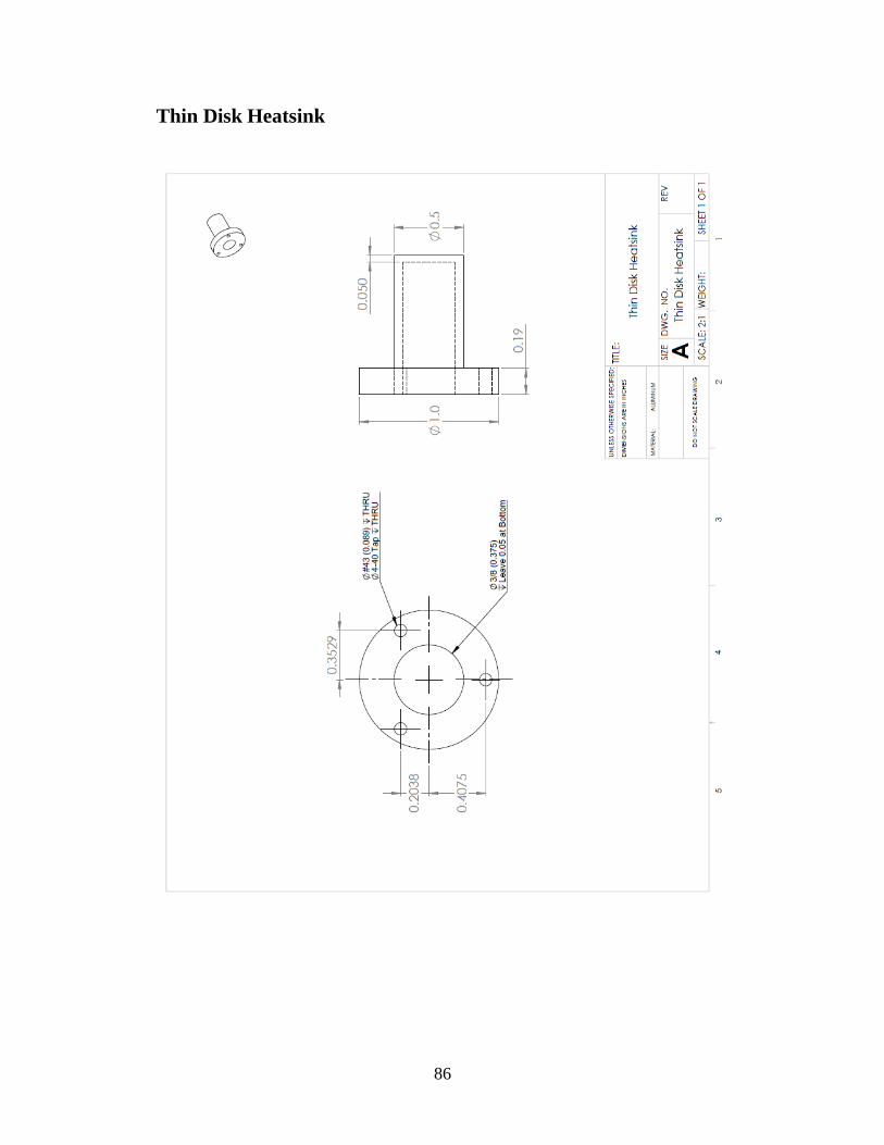
86
Thin Disk Heatsink
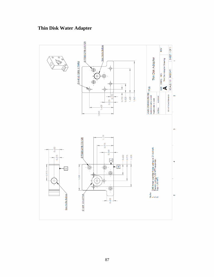
87
Thin Disk Water Adapter
88
References
[1] A. Killi, I. Zawishcha, D. Sutter, J. Kleinbauer, S. Schad, J. Neuhaus and C.
Schmitz, "Current status and development trends of disk laser technology,"
Solid State Lasers XVII: Technology and Devices, vol. Proceedings of SPIE
6871, no. 68710L, 2008.
[2] K. Scholle, S. Lamrini, P. Koopmann and P. Fuhrberg, "2 μm Laser Sources
and Their Possible Applications," Frontiers in Guided Wave Optics and
Optoelectronics, 2010.
[3] Y. Kalisky, The Physics and Engineering of Solid State Lasers, Bellingham:
SPIE, 2005, pp. 149-153.
[4] A. Siegman, Lasers, Palo Alto, CA: University Science Books, 1986, p. 66.
[5] W. Koechner, Solid-State Laser Engineering, vol. 6th, New York, NY:
Springer Science+Business Media, Inc., 2006, pp. 81, 94-101, 219-225, 282,
458-473.
[6] M. Javadi-Dashcasan and F. Hajiesmaeilbaigi, "Optimizing the Yb:YAG thin
disc laser design parameters," Optics Communications, vol. 281, no. 18, pp.
4753-4757, 2008.
[7] A. Giesen, A. Voss, K. Wittig, U. Brauch and H. Opeower, "Scalable concept
for diode-pumped high-power solid-state lasers," Applied Physics B, vol. 58,
no. 5, pp. 365-372, May 1994.
[8] A. Giesen, "Results and scaling laws of thin-disk lasers," Solid State Lsers
XIII: Technology and Devices, 8 July 2004.

89
[9] A. Tyler, E. Korczynski and K. Sumantri, "Diode-Pumped Solid-State
Lasers: Edge pumping drives slab-laser performance," 03 01 2000. [Online].
Available: http://www.laserfocusworld.com/articles/print/volume-36/issue-
3/features/diode-pumped-solid-state-lasers-edge-pumping-drives-slab-laser-
performance.html.
[10] R. Xu, L. Xu, L. Hu and J. Zhang, "Structural Origin and Laser Performance
of Thulium-Doped Germanate Glasses," J. Phys. Chem. A, vol. 115, no. 49,
pp. 14163-14167, 15 November 2011.
[11] L. Esterowitz, "Diode Pumped Holmium, Thulium And Erbium Lasers
Between 2 and 3um Operating CW At Room Temperature," 1989.
[12] X. Zhu, Measured data of Thulium3+ Germanate Absorption and Emission
Cross Section Data.
[13] R. Paschotta, "Doping Concentration," RP Photonics Consulting GmbH,
[Online]. Available: https://www.rp-
photonics.com/doping_concentration.html.
[14] K. Contag, M. Karszewski, C. Stewen, A. Giesen and H. Hugel, "Theoretical
modelling and experimental investigations of the diode-pumped thin-disk
Yb:YAG laser," Quantum Electronics, vol. 29, no. 8, pp. 697-703, 1999.
[15] A. Giesen and J. Speiser, "Fifteen Years of Work on Thin-Disk Lasers:
Results and Scaling Laws," IEEE journal of Selected Topics in Quantum
Electronics, vol. 13, no. 3, May 2007.
[16] J. Zuclich, D. Lund and B. Stuck, "Wavelength dependenc of ocular damage
thresholds in the near-IR to far-IR tansition region: proposed revisions to
MPEs," Health Physics, vol. 92, January 2007.

90
[17] G. M. Hale and M. R. Querry, "Optical cosntants of water in the 200nm to
200um wavelength region," Appl. Opt., vol. 12, pp. 555-563, 1973.
[18] J. Dong, M. Bass, Y. Mao, P. Deng and F. Gan, "Dependence of the Yb3+
emission cross section and lifetime on temperature and concentration in
yttrium aluminum garnet," Journal of the Optical Society of America B, vol.
20, no. 9, pp. 1975-1979, 2003.
[19] Q. Liu, X. Fu, M. Gong and L. Huang, "Effects of the temperature
dependence of absorption coefficients in edge-pumped Yb:YAG slab lasers,"
Journal of the Optical Society of America B, vol. 24, no. 9, pp. 2081-2089,
2007.
[20] J. E. Shelby, "Viscosity and Thermal Expansion of Alkali Germanate
Glasses," Journal of the American Ceramic Society, vol. 57, no. 10, pp. 436-
439, October 1974.
[21] H. Weber and N. Hodgson, Laser Resonators and Beam Propagation, vol.
2nd, New York, NY: Spirnger Science+Business Media, Inc, 2005, pp. 261-
264.
[22] D. Vukobratovich and S. Vukobratovich, Introduction to Opto-Mechanical
Design, Tucson: Society of Photo Optical, 1993, p. 249.
[23] S. Vatnik, I. Vedin, M. Segura and X. Mateos, "Efficient thin-disk Tm-laser
operation based on Tm:KLu(W04)2/KLu(WO4)2 epitaxies," Optics Letters,
vol. 37, no. 3, pp. 356-358, 2012.
[24] J. Wu, Z. Yao, J. Zong and S. Jiang, "Highly efficient high-power thulium-
doped germanate glass fiber laser," Optics Letters, vol. 32, no. 6, pp. 638-
640, 2007.

91
[25] Q. Fang, W. Shi, K. Kieu, E. Petersen, A. Chavez-Pirson and N.
Peyghambarian, "High power and high energy monolithic single frequency
2um nanosecond pulsed fber laser by using large core Tm-doped germanate
fibers: experiment and modeling," Optics Express, vol. 20, no. 15, pp. 16410-
16420, 2012.
[26] M. Najafi and A. Sepehr, "Simulation of thin disk laser pumping process for
temperature dependent Yb:YAG property," Optics Communications, vol.
282, no. 20, pp. 4103-4108, 15 October 2009.
[27] E. Bastow, "Indium-Copper Intermetallics in Soldering," 13 January 2012.
[Online]. Available: http://www.indium.com/blog/indium-copper-
intermetallics-in-soldering.php.