Development of a Global Slope Dataset for Development of a Global Slope Dataset for Estimation of Landslide Occurrence Estimation of Landslide Occurrence Resulting from EarthquakesResulting from Earthquakes

Open-File Report 2007-1188Open-File Report 2007-1188

U.S. Department of the InteriorU.S. Department of the InteriorU.S. Geological SurveyU.S. Geological Survey

Development of a Global Slope Dataset for Estimation of Landslide Occurrence Resulting from Earthquakes

By Kristine L. Verdin, Jonathan Godt, Chris Funk, Diego Pedreros, Bruce Worstell, and James Verdin

Open-File Report 2007–1188

U.S. Department of the Interior U.S. Geological Survey

U.S. Department of the Interior DIRK KEMPTHORNE, Secretary

U.S. Geological Survey Mark D. Myers, Director

U.S. Geological Survey, Reston, Virginia 2007

For product and ordering information: World Wide Web: http://www.usgs.gov/pubprod Telephone: 1-888-ASK-USGS

For more information on the USGS—the Federal source for science about the Earth, its natural and living resources, natural hazards, and the environment: World Wide Web: http://www.usgs.gov Telephone: 1-888-ASK-USGS

Any use of trade, product, or firm names is for descriptive purposes only and does not imply endorsement by the U.S. Government.

Although this report is in the public domain, permission must be secured from the individual copyright owners to reproduce any copyrighted material contained within this report.

Suggested citation: Verdin, K.L., Godt, J.W., Funk, C., Pedreros, D., Worstell, B., Verdin, J., 2007, Development of a global slope dataset for estimation of landslide occurrence resulting from earthquakes: Colorado: U.S. Geological Survey, Open-File Report 2007-1188, 25 p.

ii

iii

Contents Contents .............................................................................................................................................................................. iii Abstract................................................................................................................................................................................1 1. Introduction .....................................................................................................................................................................1 2. Data...................................................................................................................................................................................2 3. Methods ...........................................................................................................................................................................3

3.1 Slope Summary Statistics .......................................................................................................................................4 3.2 Elevation summary statistics..................................................................................................................................5 3.3 Critical Void Threshold ............................................................................................................................................6 3.4 Filling of Void Areas..................................................................................................................................................6 3.5 Extrapolating the Data Sets beyond 60° North....................................................................................................8

4. Discussion........................................................................................................................................................................8 5. Conclusions .....................................................................................................................................................................8 References Cited ................................................................................................................................................................9 Figures Figure 1. Distribution of finished SRTM 1-degree tiles used in the processing...................................................10 Figure 2. Percent voids summarized by one-degree tile..........................................................................................11 Figure 3. Example SRTM data for tile N40W110. .......................................................................................................12 Figure 4. Distribution tiles for GTOPO30.. ....................................................................................................................13 Figure 5. 3-by-3 processing kernel used in the calculation of slope. ....................................................................14 Figure 6. Location of sample points used in comparison of EDNA and SRTM slopes........................................15 Figure 7. SRTM skill compared with slopes derived from EDNA............................................................................16 Figure 8. Ratio of STRM mean slope and GTOPO30 slopes. ....................................................................................17 Figure 9. Best neighbor correction schema. ..............................................................................................................18 Figure 10. Sample east-west transects for the ‘best neighbor’ fill algorithm. ......................................................19 Figure 11. Sample SRTM and estimated 90th percentile fields based on GTOPO30............................................20 Figure 12. Examples of filled tile, long 100°W, lat 90°N, 90th percentile slope .....................................................21

Tables Table 1. Distribution of void areas................................................................................................................................22 Table 2. Lengths of Degrees of the Parallel ...............................................................................................................23 Table 3. Lengths of Degrees of the Meridian ............................................................................................................24 Table 4. Comparison of the EDNA and SRTM-derived slopes. ...............................................................................25

Development of a Global Slope Dataset for Estimation of Landslide Occurrence Resulting from Earthquakes

By Kristine L. Verdin1, Jonathan Godt2, Chris Funk3, Diego Pedreros3,Bruce Worstell1, and James Verdin4

Abstract Landslides resulting from earthquakes can cause widespread loss of life and damage to

critical infrastructure. The U.S. Geological Survey (USGS) has developed an alarm system, PAGER (Prompt Assessment of Global Earthquakes for Response), that aims to provide timely information to emergency relief organizations on the impact of earthquakes. Landslides are responsible for many of the damaging effects following large earthquakes in mountainous regions, and thus data defining the topographic relief and slope are critical to the PAGER system. A new global topographic dataset was developed to aid in rapidly estimating landslide potential following large earthquakes. We used the remotely-sensed elevation data collected as part of the Shuttle Radar Topography Mission (SRTM) to generate a slope dataset with nearly global coverage. Slopes from the SRTM data, computed at 3-arc-second resolution, were summarized at 30-arc-second resolution, along with statistics developed to describe the distribution of slope within each 30-arc-second pixel. Because there are many small areas lacking SRTM data and the northern limit of the SRTM mission was lat 60ºN., statistical methods referencing other elevation data were used to fill the voids within the dataset and to extrapolate the data north of 60º. The dataset will be used in the PAGER system to rapidly assess the susceptibility of areas to landsliding following large earthquakes.

1. Introduction The U.S. Geological Survey’s (USGS) National Earthquake Information Center in Golden,

Colorado, reports on more than 30,000 earthquakes a year, 25 of which usually cause significant damage, injuries, or fatalities. Historically, the USGS has relied on the working experience of on-duty seismologists to estimate the impact of events and determine if Federal and international aid agencies should be alerted. The Prompt Assessment of Global Earthquakes for Response (PAGER) system is designed to provide a near-real time estimate to governmental and non-governmental relief organizations, and the media of an earthquake’s effects anywhere in the world. PAGER is an automated system designed to estimate the effects of significant earthquakes on humans. One

1 Science Applications International Corporation (SAIC), contractor to the U.S. Geological Survey (USGS) Center for Earth Resources Observation and Science, Sioux Falls, SD. Work performed under USGS contract 03CRCN0001. 2 USGS Landslides Hazards Group, Golden, CO 3 University of California, Santa Barbara, CO 4 USGS Center for Earth Resources Observation and Science, Sioux Falls, SD

1

component of the global system is development of estimates of the potential for earthquake-induced landslides.

The method to estimate the potential impact of earthquake-induced landslides in near-real

time is under development, and one approach that has been suggested is to couple an estimate of ground-shaking intensity with a simplified Newmark slope-stability analysis (Newmark, 1965; Godt and others, 2006). The simplified Newmark analysis calculates a critical (or yield) acceleration above which ground displacement is to be expected. Wherever the estimated Peak Ground Acceleration (PGA) produced as part of the PAGER system exceeds the yield acceleration, landsliding is assumed to occur. Whatever approach is ultimately adopted to assess the potential impact from earthquake-triggered landslides, a global database of topographic slope will be required.

To this end, we undertook to develop a global slope dataset based on the Shuttle Radar

Topography Mission (SRTM) Digital Elevation Model (DEM). The SRTM DEM, with its global 3-arc-second resolution (approximately 90 meters at the equator), formed the basis for all data development efforts to support the PAGER system. Along with the global slope dataset at the publicly-available 3-arc-second resolution of the SRTM DEM, additional data layers were developed at the coarser resolution of 30 arc-seconds (approximately 1 km at the equator) to support the PAGER system. These datasets describe the distribution of the elevation and slope within each 30-arc-second pixel, and include layers such as mean slope, mean elevation, 90th quantile slope, etc. In all, 15 global data layers were developed which describe the elevation and slope data derived from the SRTM DEM. The development of these datasets is described in this report.

2. Data The derivative layers developed for this effort were based on the SRTM DEM. The SRTM

was a collaborative effort by the National Aeronautics and Space Administration (NASA) and the National Geospatial-Intelligence Agency (NGA), with participation of the German and Italian space agencies, to generate a near-global DEM of the Earth using radar interferometry. In February 2000, the SRTM was the primary payload aboard the Space Shuttle Endeavour and successfully acquired terrain information between lat 56°S. and 60°N., approximately 80 percent of the Earth’s land mass. The SRTM data acquired in February 2000 were processed into Digital Terrain Elevation Data (DTED®) by NASA’s Jet Propulsion Laboratory (JPL). Details of the SRTM mission and the data can be found in Farr and Kobrick (2000).

Following production of the unfinished SRTM data, contractors working for the NGA produced the finished SRTM products. The finished products differ from the unfinished data in several ways: small voids, or areas within the dataset which had no elevation information, were filled, lakes were flattened, rivers were monotonically stepped down and coastlines were delineated (Slater and others, 2006).

The SRTM DTED® data were divided into 1-degree by 1-degree tiles for processing, storage, and retrieval. The elevation values are rounded to the nearest meter and are referenced to mean sea level as defined by the WGS 84 / EGM 96 geoid. Elevations in the SRTM dataset are not necessarily ground elevations; instead, they represent the elevations of the reflective surface of the radar return. The finished SRTM are made freely available to the public through the USGS Center for Earth Resources Observation and Science (EROS) Seamless Data Distribution System (http://seamless.usgs.gov/). Data are available for the globe at a resolution of 3 arc-seconds and for

2

the United States at 1 arc-second. The data are also available in a tiled format from NASA’s ftp site (ftp://e0srp01u.ecs.nasa.gov/srtm/version2/).

The finished SRTM data were used in this analysis. Data were processed using the SRTM’s 1-degree tile structure. The data were converted from the DTED® format into Arc Grid format. This resulted in each one-degree tile consisting of 1,200 rows and 1,200 columns with a cell spacing of 3 arc-seconds. A total of 14,277 1-degree tiles were processed for this effort. The distribution of the available SRTM tiles is shown in Figure 1.

The finished SRTM data have many of the smaller voids filled, but many of the 1-degree tiles still contain voids (Hall and others, 2005). Shown in Figure 2 is the distribution of voids that remain in the finished SRTM product. Table 1 also summarizes this information. Of all tiles, 28 percent contain no voids and 63 percent are less than one percent void by area. Of the 14,277 one-degree tiles, only 1,322 contain void areas in excess of one percent.

Efforts are underway, through contractors to NGA, to systematically fill the voids in the finished SRTM product. A completion date for this work is unknown, and it has not been decided whether the completed product will be made available to the public. To ensure that our results were based on publically available data, the work described in this paper uses the SRTM data with the voids intact. In sections 3.3 and 3.4, we discuss procedures to identify the effect of and compensate for the voids in generation of the various data products.

3. Methods The SRTM DEM has a resolution of 3 arc-seconds, but the summary data layers developed

to support the PAGER system were developed at a reduced, more globally manageable resolution of 30 arc-seconds. As a result, each tile of the SRTM DEM data consists of 1200 rows by 1200 columns at 3 arc-second resolution, and each tiled data layer used in our study consists of 120 rows by 120 columns at 30 arc-second resolution (see Figure 3). Data were processed on a tile basis and the resulting data layers were merged at the end of processing to assemble the global data layers. Because the layers were large, the data were composited on twenty-seven 40 degree by 50 degree tiles to accommodate the procedures used to compensate for the voids in the data, which rely heavily on GTOPO30 data (Gesch and others, 1999). These tiles correspond to the spatial extent of the GTOPO30 distribution packages (Figure 4). In all, 15 data layers were developed:

1. Mean slope

2. Minimum slope

3. Maximum slope

4. 10th quantile slope

5. 30th quantile slope

6. 50th quantile slope (median)

7. 70th quantile slope

8. 90th quantile slope

9. Standard deviation of the slope

10. Mean elevation

11. Median elevation

12. Minimum elevation

13. Maximum elevation

3

14. Elevation range

15. Standard deviation of elevation

3.1 Slope Summary Statistics

The SRTM DEM posed a unique challenge in the calculation of slopes. The elevation values are reported in meters and the cell size of the DEM is in units of decimal degrees (3 arc-seconds or 0.00083 decimal degrees). Since slope can be simplistically thought of as “rise over run,” the units used for elevations and for ground distances need to be consistent to produce a correct slope calculation. Most standard Geographic Information System (GIS) packages have accommodation for adjusting one unit to be consistent with the other. For example, in the implementation of the slope algorithm within ArcGIS (Burke and others, 2004), the z-factor parameter is available in order to adjust the units of the elevations (Z) to match the ground units (X and Y).

The problem arises with the use of the SRTM data with ground units of decimal degrees. There is not a simple factor that will convert decimal degrees to units of meters (the z-units of the SRTM) for the entire globe, because the length of one degree varies depending on its latitudinal location. At the equator, a one-degree by one-degree block is reasonably square when converted to units of meters (111,321 meters in the x-direction by 110,567 meters in the y-direction (Robinson and others, 1969)), but closer to the poles the distances in the x-direction grow smaller as a function of the cosine of latitude, owing to convergence of the meridians.

Most GIS packages, ArcGIS included, operate only on square pixels, and so using a factor to adjust the x, y, or z dimensions to a common unit is not possible. One solution would be to project each SRTM tile into an equidistant projection, such as the Azimuthal Equidistant projection (ESRI, 1994), calculate the slopes in this equidistant projection and then project the data back into a geographic framework. Because the goal of this work is to develop accurate summary statistics at 30-arc-seconds describing the underlying 3-arc-second data, the additional smoothing that would result from such a series of projections, along with the additional processing time, argued for an alternative solution.

We calculated slope in the geographic framework through a straightforward application of the underlying slope equation. This equation allows for different cell sizes in the x and y directions. Slope, the first derivative of the elevation surface, is defined by a plane tangent to the surface as modeled by the DEM at any given point. The derivative is calculated locally for each cell in the grid by computations made within a 3-by-3 kernel. Slope is defined by:

22 )/()/(tan YZXZS δδδδ += (Eq. 1)

where S is the slope in degrees, Z is the elevation and X & Y are the coordinate axes. Using the symbology defined for each 3-by-3 roving window shown in Figure 5, the changes of elevation in the X & Y directions are calculated (Burrough, 1986) using:

[ ] [ ]X

ZZZZZZXZ jijijijijiji

ji δδδ

8)2()2(

/ 1,1,11,11,1,11,1,

−−−+−−++++ ++−++= (Eq. 2)

[ ] [ ]Y

ZZZZZZYZ jijijijijiji

ji δδδ

8)2()2(

/ 1,11,1,11,11,1,1,

−−−−++−+++ ++−++= (Eq. 3)

4

Slopes were calculated using the 3-by-3 roving window (Figure 5) on a tile-by-tile basis through application of Equations 1, 2, and 3. Voids were dealt with in each 3-by-3 window. If any of the 8 pixels surrounding the central pixel were void, the elevation of the central pixel was used in place of the void pixel. If the central pixel was itself void, no valid slope would be calculated and the value for that pixel would be void. In 3-by-3 windows with several voids, the use of the central pixel to fill the void pixels has the result of smoothing the derived slopes. Additionally, to deal with the edge-effects of processing on a tile-by-tile basis, the outermost rows and columns were replicated in order to provide a valid 3-by-3 window at the edge of the tile. This resulted in each tile, for processing, having 1202 rows by 1202 columns; however, the resulting slope dataset was trimmed back to the original 1200 rows by 1200 columns.

Because the SRTM data are in the geographic coordinate system, the linear distances between postings change as the latitude changes. To convert the ground units from decimal degrees into meters, lookup tables describing the distance in meters for each degree of longitude were used to convert the 3-arc-second spacing in the X-direction (Table 2) and Y-direction (Table 3) into units of meters. The distances in the X-direction vary considerably, with one degree of longitude at the equator equaling 111,321 meters, whereas at 59 degrees north or south latitude, the same one degree of longitude equates to only 57,478 meters. The variation of lengths in meters in the Y-direction is not as dramatic, varying from 111,567 meters at the equator to 111,406 meters at 59 degrees north or south. These average distances between postings were used as the δX and δY factors in the slope equations.

Data procedures were developed in the Python programming language (van Rossum, 2006) and related add-on modules to facilitate array processing and analysis. These modules include the numeric and numarray modules that provide the basic array processing and analysis capabilities, the matplotlib add-on module, which is an analysis and graphing module that supports a variety of methods to facilitate data analysis, and the Geospatial Data Abstraction Library (GDAL) module. Because the local repository SRTM data are stored in ArcGIS GRID format, the GDAL module, which also has methods available from within Python, was used to read the SRTM data and make the data accessible as a numeric array.

To calculate the distribution of slope values, aggregation blocks were created for each tile. Each aggregation block was 10 cells by 10 cells, resulting in 120 by 120 aggregation blocks for each tile (see Figure 3). The minimum, maximum, mean, and standard deviation were computed for each block using functions within the numarray module. The percentiles were computed for the 10th, 30th, 50th (median), 70th, and 90th percentile using a routine for computing percentiles within the matplotlib module.

3.2 Elevation summary statistics

Elevation summary statistics were calculated by a straightforward application of ArcGIS

modules. The SRTM elevation values are stored by ArcGIS as integer meters. The ZONAL functions within ArcGIS were used to summarize the mean, median, minimum, maximum, and standard deviation for each 30-arc-second pixel within each 1-degree tile. The range was calculated as the difference between the maximum and minimum elevations for each 30-arc-second pixel.

5

3.3 Critical Void Threshold

The calculation of slope values at 3-arc-second resolution and the development of all the

summary statistic layers at 30-arc-second resolution were done without regard to the presence of voids in the data. As can be seen from Figure 2, most of the 1-degree tiles have less than one percent voids by area. However, some voids are large. The question, therefore, is whether or not the presence of voids in the data set affects the calculation of the summary statistics at 30-arc-second resolution and, if so, at what level of void area the summary statistics are affected.

To assess the effect of void area on the calculation of the summary statistics, a comparison was made between mean slopes at 30-arc-second resolution calculated from two different sources. The Elevation Derivatives for National Applications (EDNA, Verdin, 2000) is a multi-layer database of standard DEM derivatives for the United States, one of which is a slope layer. The EDNA, with its 30-meter (1 arc-second) resolution, is derived from the National Elevation Dataset (NED, Gesch and others, 2002) and is seamless; there are no voids in the DEM or the derivative layers. We compared the mean slopes from the EDNA slope layer aggregated to 30 arc-seconds with those derived from the 3 arc-second SRTM summarized at 30 arc-seconds. The EDNA layer provided, in essence, a truth dataset, since there are no voids in the slope layer and it is derived from the best available DEMs for the United States. We can expect differences between the slopes derived using each dataset, owing to the different collection methodologies of the underlying DEMs; however, we hoped to determine a critical void threshold at which the presence of the voids significantly impaired the calculation of the summary statistics.

Sampling locations were determined by selecting every 30-arc-second SRTM pixel within the conterminous United States in which the void area exceeded 15 percent. These pixels were converted to a point dataset and this dataset was used to sample the underlying EDNA and SRTM slope grids. The sample locations are shown in Figure 6. A total of 25,249 samples were collected from the EDNA aggregated mean slope and the SRTM 30-arc-second mean slope layers. The differences in mean slopes between the two datasets were then calculated and summarized by void area (Table 4 and Figure 7).

Summary statistics calculated for 30-arc-second pixels with voids in excess of 35 to 40 percent do not correlate well with the EDNA-derived statistics (Figure 7). Accordingly, a threshold of 33 percent was chosen to define the locations where the summary statistics calculated using the raw SRTM could be considered erroneous due to the presence of voids. The 30-arc-second pixels identified in this manner (voids in excess of 33 percent) were flagged for replacement. The method of estimating an improved set of summary statistics for these flagged pixels is discussed in Section 3.4.

3.4 Filling of Void Areas

Prior to the release of the SRTM data, the best available, globally consistent DEM was

GTOPO30 (http://eros.usgs.gov/products/elevation/gtopo30/gtopo30.html). This dataset, with its cell size of 30 arc-seconds, was derived from various sources, mostly of a cartographic base. In order to fill the void areas within the SRTM, we analyzed the correspondence between the GTOPO30 and the SRTM layers and used these relationships to fill out the SRTM layer.

Analysis of the relationships between the GTOPO30 and SRTM slope fields revealed strong locally systematic relationships. The higher resolution of the SRTM tended to produce similar but more extreme values. Exploratory analysis also demonstrated that a single one-pixel shift between

6

the two images could often dramatically increase their correspondence. These observations led us to develop a two-step filling procedure.

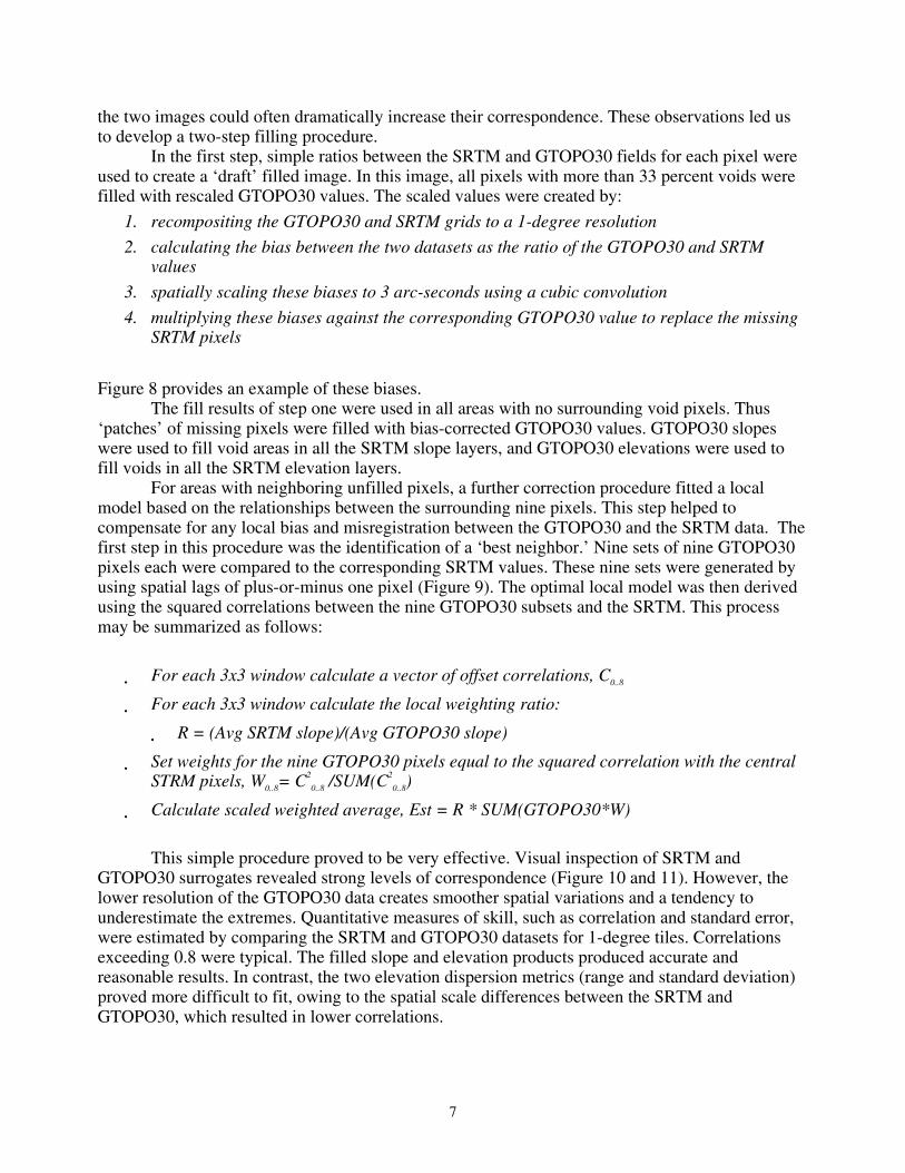
In the first step, simple ratios between the SRTM and GTOPO30 fields for each pixel were used to create a ‘draft’ filled image. In this image, all pixels with more than 33 percent voids were filled with rescaled GTOPO30 values. The scaled values were created by:

1. recompositing the GTOPO30 and SRTM grids to a 1-degree resolution

2. calculating the bias between the two datasets as the ratio of the GTOPO30 and SRTM values

3. spatially scaling these biases to 3 arc-seconds using a cubic convolution

4. multiplying these biases against the corresponding GTOPO30 value to replace the missing SRTM pixels

Figure 8 provides an example of these biases. The fill results of step one were used in all areas with no surrounding void pixels. Thus

‘patches’ of missing pixels were filled with bias-corrected GTOPO30 values. GTOPO30 slopes were used to fill void areas in all the SRTM slope layers, and GTOPO30 elevations were used to fill voids in all the SRTM elevation layers.

For areas with neighboring unfilled pixels, a further correction procedure fitted a local model based on the relationships between the surrounding nine pixels. This step helped to compensate for any local bias and misregistration between the GTOPO30 and the SRTM data. The first step in this procedure was the identification of a ‘best neighbor.’ Nine sets of nine GTOPO30 pixels each were compared to the corresponding SRTM values. These nine sets were generated by using spatial lags of plus-or-minus one pixel (Figure 9). The optimal local model was then derived using the squared correlations between the nine GTOPO30 subsets and the SRTM. This process may be summarized as follows:

• For each 3x3 window calculate a vector of offset correlations, C0..8

• For each 3x3 window calculate the local weighting ratio:

• R = (Avg SRTM slope)/(Avg GTOPO30 slope)

• Set weights for the nine GTOPO30 pixels equal to the squared correlation with the central STRM pixels, W0..8= C2

0..8 /SUM(C2

0..8)

• Calculate scaled weighted average, Est = R * SUM(GTOPO30*W)

This simple procedure proved to be very effective. Visual inspection of SRTM and

GTOPO30 surrogates revealed strong levels of correspondence (Figure 10 and 11). However, the lower resolution of the GTOPO30 data creates smoother spatial variations and a tendency to underestimate the extremes. Quantitative measures of skill, such as correlation and standard error, were estimated by comparing the SRTM and GTOPO30 datasets for 1-degree tiles. Correlations exceeding 0.8 were typical. The filled slope and elevation products produced accurate and reasonable results. In contrast, the two elevation dispersion metrics (range and standard deviation) proved more difficult to fit, owing to the spatial scale differences between the SRTM and GTOPO30, which resulted in lower correlations.

7

The filling process was carried out on the 40 degree by 50 degree GTOPO30 grids, and slopes were calculated from the GTOPO30 with an IDL port of the same code used to estimate slope values from the STRM (see Section 3.1).

3.5 Extrapolating the Data Sets beyond 60° North

A process similar to step one of the void-filling procedure was used to extend the summary data layers beyond 60°N. A bivariate regression model was constructed for each of the nine GTOPO30 tiles that extended beyond 60°N, covering the area from 40°N to 90°N. For the areas between 40°N and 60°N, where both SRTM and GTOPO30 data are present, both datasets were averaged by 1-degree blocks, and a regression carried out between the two aggregated fields. For slope fields, a bias correction was estimated, based on the GTOPO30 slopes. Similarly, GTOPO30 elevations formed the basis for correcting elevation fields. The regression models developed in this manner were then applied to the areas north of 60° using the GTOPO30 as the independent variable.

4. Discussion This database will provide the topographic information necessary to develop and test a

global system to provide a rapid assessment of the impacts of earthquake-induced landslides. The calculation of slope and elevation statistics from the raw 3-arc-second SRTM data was a straightforward procedure. The filling process, to replace the void pixels and extend the dataset north of lat 60ºN, was more susceptible to problems – including the development of discontinuities in the data or the introduction of biases. We found that the two-step procedure for filling voids and the bivariate regression model technique to extrapolate the data north of 60º produced adequate results. In particular, the procedure to extrapolate the data north of 60º removed some large scale biases between the GTOPO30 and SRTM data, and a visual comparison suggests a reasonable fit at coarse levels of analysis (Figure 12, left panel). However, the GTOPO30 elevations exhibit substantial discontinuities, owing to the differing physical and cartographic natures of GTOPO30 and SRTM data. At smaller scales, systematic differences in the scale of the data are apparent (Figure 12, right panel). The GTOPO30 dataset has a much coarser resolution than the SRTM data, and presents a less variable landscape. Again, this scale discrepancy was most significant for the range and standard deviation files.

5. Conclusions A new global topographic dataset has been created to assist in estimating the potential for

large landslides following large earthquakes. This global dataset was developed from the 3-arc-second SRTM data and consists of 15 derivative layers at 30-arc-second resolution. New techniques were developed to fill the voids in the derivative layers as well as extrapolate the layers beyond lat 60°N (the northernmost limit of the SRTM data). Data were filled and extrapolated using bivariate regression models with GTOPO30 derivatives as the independent variable. Because of the different collection methods and resolutions of the SRTM and the GTOPO30 data, the fit between the two datasets is adequate, but not optimal.

These derivative layers will be used in developing the landslide potential models which will be implemented worldwide. The techniques for estimating landslide potential are still being

8

developed and this database will help define the critical parameters for assessing landslide potential. The database is at 30-arc-second resolution, as is GTOPO30, but the summary statistics from the underlying 3-arc-second SRTM data will provide the models with additional information which was not available previously which may enable much broader application.

References Cited Burke, R., Napoleon, E., and Ormsby T., 2004, Getting to Know ArcGIS Desktop: Redlands,

Calif., ESRI Press, 588 p. Burrough, P.A., 1986, Principles of Geographical Information Systems for Land Resources

Assessment: New York, Oxford University Press, p. 50. Environmental Systems Research Institute (ESRI), 1994, Map Projections, Georeferencing Spatial

Data: Redlands, Calif., ESRI, Inc. Farr, T.G., and Kobrick, M., 2000, Shuttle Radar Topography Mission produces a wealth of data:

Eos, Transactions, American Geophysical Union, v. 81, p. 583-585. Gesch, D.B., Verdin, K.L., Greenlee, S.K., 1999, New land surface digital elevation model covers

the Earth: Eos, Transactions, American Geophysical Union v. 80, no. 6, p. 69-70. Gesch, D., Oimoen, M., Greenlee, S., Nelson, C., Steuck, M., and Tyler, D., 2002, The National

Elevation Dataset: Photogrammetric Engineering and Remote Sensing, v. 68, no. 1, January, 2002.

Godt, J.W., Verdin, K.L., Jibson, R.W., Wald, D.J., Earle, P.S., and Harp, E.L., 2006, Rapid global assessment of the societal impacts of earthquake induced landsliding: Eos, Transactions, American Geophysical Union, v. 87, no. 36, p. H32A-04.

Hall, O., Falorni, G., and Bras, R.L., 2005, Characterization and quantification of data voids in the shuttle Radar topography mission data: IEEE Geoscience and Remote Sensing Letters, v. 2, no. 2, p. 177.

Newmark, N.M., 1965, Effect of earthquakes on dams and embankments: Geotechnique, v. 15, p. 139-160.

Robinson, A.H., and Sale, R.D., 1969, Elements of Cartography, 3rd edition: New York, John Wiley & Sons, Appendix D.

Slater, J.A., Garvey, G., Johnston, C., Haase, J., Heady, B., Kroenung, G., and Little, J., The SRTM Data “Finishing” Process and Products: Photogrammetric Engineering and Remote Sensing, v. 72, no. 3, p. 237-248, March, 2006.

Van Rossum, G., 2006, Python Reference Manual, Python Software Foundation, available at http://docs.python.org/ref/, last accessed on November 30th, 2006.

Verdin, K.L., 2000, Development of the National Elevation Dataset Hydrologic Derivatives (NED-H), in Proceedings, 20th Annual ESRI International User Conference, San Diego California, July 2000.

9

Figure 1. Distribution of finished SRTM 1-degree tiles used in the processing. A total of 14,277 tiles were available. The limits of the SRTM data collection were from lat 56°S to 60°N.

10

Figure 2. Percent voids summarized by one-degree tile. Many of the tiles (3,965 out of 14,277 one-degree tiles or 28 percent) have no voids after the finishing process. However, the majority of the tiles still contain voids, with some voids of significant extent. The maximum percent of tile coverage containing voids is 73 percent.

11

Figure 3. Example data for tile N40W110. Top figures show the full resolution (3-arc-second) SRTM slope data for the tile. The lower figures show the mean slope data summarized by 30-arc-second pixel. Other statistics calculated in a similar frame framework include the minimum, maximum, median, and others.

12

Figure 4. Distribution tiles for GTOPO30. This 40-degree by 50-degree tile structure was used to composite the 1-degree SRTM tiles. Additionally, the two-stage void-filling algorithm operated under this tile structure.

13

Zi-1,j+1 Zi,j+1 Zi+1,j+1

Zi-1,j Zi,j Zi+1,j

Zi-1,j-1 Zi,j-1 Zi+1,j-1

Figure 5. 3-by-3 processing kernel used in the calculation of slope.

14

Figure 6. Location of sample points used in comparison of EDNA and SRTM slopes. All pixels with void area in excess of 15 percent were selected for comparison. A total of 25,249 points was used.

15

SRTM skill (r) when compared with EDNA slope estimates at 30 arc-seconds

0.4

0.5

0.6

0.7

0.8

15% 20% 25% 30% 35% 40% 45% 50% 55% 60% 65% 70% 75% 80%

Percent Void Categories

Cor

rela

tion

(r)

Figure 7. SRTM [skill] compared with slopes derived from EDNA. A threshold of 33 percent was set to select those pixels which are significantly impacted by the presence of voids.

16

Figure 8. Ratio of STRM mean slope and GTOPO30 slopes for a region of the southwestern United States. Values were stretched from 0.5 (dark blue) to 3.0 (dark red).

17

9 sets of 9 pixels used to detect offset correlations

1 2 3

4 5 6

7 8 9

Central box contains SRTM

Figure 9. Best neighbor correction schema. The numbers (1 to 9) correspond to the central pixel of the candidate 3-by-3 block.

18

Figure 10. Sample east-west transects for the ‘best neighbor’ fill algorithm drawn from long 20-21°E and lat 39-40° N. Blue lines designate the SRTM mean slope values. Red lines show the values estimated from GTOPO30 slopes.

19

Figure 11. Sample SRTM 90th percentile fields (left) and estimated 90th percentile fields based on GTOPO30. Yellow hues denote high slopes. 1-degree tile centered at long 113°30′W and lat 32°30′N.

20

Figure 12. Examples of filled tile, long 100°W, lat 90°N, 90th percentile slope. The filling procedure removes systematic bias (left). Variations in resolution are still apparent (right).

21

Table 1. Distribution of void areas. Of the 14,277 one-degree tiles, over 90 percent have void areas of 1 percent or less. The remaining void areas are, at times, of significant size. The spatial distribution of these voids is shown in Figure 2.

Percent of area containing voids (v)

Number of one-degree tiles

Percent of total

v = 0% 3965 27.8%

0% < v <= 1% 8990 63.0%

1% < v <= 5% 884 6.2%

5% < v <= 10% 223 1.6%

10% < v <= 25% 150 1.0%

v > 25% 65 0.4%

TOTAL 14277 100%

22

Table 2. Lengths of Degrees of the Parallel from Robinson and Sale (1969)

Latitude of Southwest Corner of Tile

Lengths of Degrees of the Parallel (meters)

Latitude of Southwest Corner of Tile

Lengths of Degrees of the Parallel (meters)

0 111321 30 96488

1 111304 31 95506

2 111253 32 94495

3 111169 33 93455

4 111051 34 92387

5 110900 35 91290

6 110715 36 90166

7 110497 37 89014

8 110245 38 87835

9 109959 39 86629

10 109641 40 85396

11 109289 41 84137

12 108904 42 82853

13 108486 43 81543

14 108036 44 80208

15 107553 45 78849

16 107036 46 77466

17 106487 47 76058

18 105906 48 74628

19 105294 49 73174

20 104649 50 71698

21 103972 51 70200

22 103264 52 68680

23 102524 53 67140

24 101754 54 65578

25 100952 55 63996

26 100119 56 62395

27 99257 57 60774

28 98364 58 59135

29 97441 59 57478

23

Table 3. Lengths of Degrees of the Meridian from Robinson and Sale (1969)

Latitude of Southwest Corner of Tile

Lengths of Degrees of the Meridian (meters)

Latitude of Southwest Corner of Tile

Lengths of Degrees of the Meridian (meters)

0 110567.3 30 110857.0

1 110568.0 31 110874.4

2 110569.4 32 110892.1

3 110571.4 33 110910.1

4 110574.1 34 110928.3

5 110577.6 35 110946.9

6 110581.6 36 110965.6

7 110586.4 37 110984.5

8 110591.8 38 111003.7

9 110597.8 39 111023.0

10 110604.5 40 111042.4

11 110611.9 41 111061.9

12 110619.8 42 111081.6

13 110628.4 43 111101.3

14 110637.6 44 111121.0

15 110647.5 45 111140.8

16 110657.8 46 111160.5

17 110668.8 47 111180.2

18 110680.4 48 111199.9

19 110692.4 49 111219.5

20 110705.1 50 111239.0

21 110718.2 51 111258.3

22 110731.8 52 111277.6

23 110746.0 53 111296.6

24 110760.6 54 111315.4

25 110775.6 55 111334.0

26 110791.1 56 111352.4

27 110807.0 57 111370.5

28 110823.3 58 111388.4

29 110840.0 59 111405.9

24

25

Table 4. Comparison of the slopes derived from EDNA aggregated to 30 arc-seconds and those derived from the SRTM. Thirty-three percent was selected as the break point at which the mean slopes were affected by the presence of voids.

Percent of the 30 arc-second pixel containing voids

Average squared error Variance Skill

15% 67.458 0.6458 0.8036 20% 69.542 0.6348 0.7968 25% 87.338 0.5414 0.7358 30% 95.669 0.4976 0.7054 35% 102.266 0.4630 0.6804 40% 119.976 0.3700 0.6083 45% 116.082 0.3905 0.6249 50% 128.389 0.3258 0.5708 55% 126.233 0.3371 0.5807 60% 146.872 0.2288 0.4783 65% 131.053 0.3118 0.5584 70% 146.307 0.2317 0.4814 75% 136.028 0.2857 0.5345 80% 129.814 0.3183 0.5642