Development of a Coupled Land Surface and … of a Coupled Land Surface and Groundwater Model ... by...

Development of a Coupled Land Surface and Groundwater Model

REED M. MAXWELL

Environmental Science Division, Lawrence Livermore National Laboratory, Livermore, California

NORMAN L. MILLER

Earth Sciences Division, Lawrence Berkeley National Laboratory, Berkeley, California

(Manuscript received 5 May 2004, in final form 1 December 2004)

ABSTRACT

Traditional land surface models (LSMs) used for numerical weather simulation, climate projection, andas inputs to water management decision support systems, do not treat the LSM lower boundary in a fullyprocess-based fashion. LSMs have evolved from a leaky-bucket approximation to more sophisticated landsurface water and energy budget models that typically have a specified bottom layer flux to depict the lowestmodel layer exchange with deeper aquifers. The LSM lower boundary is often assumed zero flux or the soilmoisture content is set to a constant value; an approach that while mass conservative, ignores processes thatcan alter surface fluxes, runoff, and water quantity and quality. Conversely, groundwater models (GWMs)for saturated and unsaturated water flow, while addressing important features such as subsurface hetero-geneity and three-dimensional flow, often have overly simplified upper boundary conditions that ignore soilheating, runoff, snow, and root-zone uptake. In the present study, a state-of-the-art LSM (Common LandModel) and a variably saturated GWM (ParFlow) have been coupled as a single-column model.

A set of simulations based on synthetic data and data from the Project for Intercomparison of Land-surface Parameterization Schemes (PILPS), version 2(d), 18-yr dataset from Valdai, Russia, demonstratethe temporal dynamics of this coupled modeling system. The soil moisture and water table depth simulatedby the coupled model agree well with the Valdai observations. Differences in prediction between thecoupled and uncoupled models demonstrate the effect of a dynamic water table on simulated watershedflow. Comparison of the coupled model predictions with observations indicates certain cold processes suchas frozen soil and freeze/thaw processes have an important impact on predicted water table depth. Com-parisons of soil moisture, latent heat, sensible heat, temperature, runoff, and predicted groundwater depthbetween the uncoupled and coupled models demonstrate the need for improved groundwater representa-tion in land surface schemes.

1. Introduction

Early climate simulation models used a leaky-bucketparameterization to represent land surface hydrologyas the lower boundary condition to atmospheric pro-cesses (Manabe et al. 1965). Such a simplistic descrip-tion for land surface processes in global climate models(GCMs) led to the development of land surface models(LSMs) that include vegetation, surface resistance, andsnow schemes that calculate time- and space-varyingmomentum, heat, and moisture fluxes to the lower at-mosphere (e.g., Dickinson et al. 1986; Sellers et al.1986). This was followed by LSMs with improved rep-resentations of subsurface hydrology, lateral soil mois-

ture movement, evapotranspiration (Abromopoulos etal. 1988), and continental-scale river routing (Russelland Miller 1990). At about this time, regional climatemodeling with similar LSMs began to provide higherspatial resolution (Dickinson et al. 1989; Giorgi 1990).These regional climate models are based on numericalweather prediction models coupled with global climatemodel LSMs. More recently, detailed descriptions ofsurface infiltration and lateral baseflow have been de-veloped (Famiglieti and Wood 1991; Wood et al. 1992;Liang et al. 1994). The most recent LSMs (e.g., Foley etal. 1996; Bonan 1998; Dai and Zeng 1997; Walko et al.2000; Oleson et al. 2004) have advanced to includemore detailed ecological and biogeochemical processes.

However, most LSMs to date have a parameteriza-tion at the bottom layer that is either specified as aconstant or a representation of the overlying moisturegradient. The water balance computed by land surfacemodels can be much improved by inclusion of ground-water processes and the interactive flux between the

Corresponding author address: Reed M. Maxwell, Environmen-tal Science Division, Lawrence Livermore National Laboratory(L-208), 7000 East Avenue, Livermore, CA 94550.E-mail: [email protected]

VOLUME 6 J O U R N A L O F H Y D R O M E T E O R O L O G Y JUNE 2005

© 2005 American Meteorological Society 233

JHM422

water table (WT) and the LSM lower layer. Conversely,traditional groundwater models have a simplified upperboundary condition that is externally specified and in-tended to represent fluxes of water related to processessuch as infiltration and evapotranspiration. Thesefluxes are often simplified, uncoupled, and may be av-eraged in time and space, possibly missing key dynam-ics of important land surface processes.

The Biosphere–Atmosphere Transport Scheme(BATS) assumes a constant value of 4 � 10�4 mm s�1

downward flux at the lowest soil layer (Dickenson et al.1993), and the Simple Biosphere scheme (SiB) has aparameterized downward flux as a function of gravitybased on slope (Sellers et al. 1986). During the lastseveral years, the linkage between the land surface hy-drology and the deep groundwater aquifer has receivedincreasing attention. Salvucci and Entekhabi (1995)evaluated surface and groundwater interactions with asteady-state statistical approach that showed significantshifts in evapotranspiration and runoff. Levine and Sal-vucci (1999) used a modified groundwater model toevaluate the saturated and unsaturated zones andfound that recharge was closer to observations than anuncoupled LSM with simple lower boundary condi-tions. Liang et al. (2003) developed a one-dimensionaldynamic groundwater parameterization as a function ofWT depth for a land surface model. Results indicatethat the lower LSM soil layer is wetter with this newparameterization that accounts for fluxes between theWT and this layer. This also results in higher baseflow,lower peak runoff, and decreased evapotranspiration.Yeh and Eltahir (2005) developed a lumped unconfinedaquifer model interactively coupled to a land sur-face model with a similar approach to Liang et al. (2003).

Hence, the development of a physically based anddynamically coupled land surface groundwater modelhas been proposed. The dynamics of this formulationhinges on the interactions across the LSM soil columnand a deep groundwater model (GWM). For example,as Pikul et al. (1974) demonstrated that a series of one-dimensional Richards’ equation models coupled to theBoussinesq equation could accurately represent agroundwater hydrograph. The purpose for such acoupled LSM and GWM is to determine the sensitivityof the WT and deep groundwater processes to changingclimate variables, the impact of the GWM on the LSM,and in turn the surface to atmosphere fluxes. Finally, acoupled LSM–GWM will help to better understandgroundwater and surface water interactions at a rangeof scales and their effects on water quality. In the fol-lowing section we present an approach toward devel-oping a coupled LSM–GWM, followed by a discussionof simulation and results, and finally a summary andconcluding remarks.

2. ApproachTo understand the sensitivity of an LSM with the

addition of a lower flux and deep groundwater model,

a state-of-the-art LSM and deep groundwater modelwere selected in this study. The LSM used here is thehybrid version Common Land Model (Dai et al. 2003)and the GWM is ParFlow (Ashby and Falgout 1996).The following two subsections provide brief descrip-tions of the Common Land Model and ParFlow.

a. The Common Land Model

The hybrid form of the Common Land Model (CLM)was developed as a multi-institutional code (Dai et al.2003). It is based on land surface models developed byDickinson et al. (1986), Dai and Zeng (1997), and Bo-nan (1998). Each grid tile may be partitioned into mul-tiple subgrids that define land characterizations at finespatial resolution while providing computational effi-ciency. Each grid can be subdivided into any number ofsubgrids that contain a single land-cover type, includingareas with the dominant and secondary vegetationtypes, bare soil, wetlands, and lakes. An additional landsurface type was incorporated within CLM to representan urban environment that is highly impermeable.CLM has a single vegetation canopy layer, 10 unevenlyspaced soil layers, and up to 5 snow layers. Vegetationprocesses are described as plant function types that arespecified by optical, morphological, and physiologicalproperties. The time-varying vegetation parameters in-clude the stem and leaf area indices, and the fractionalvegetation cover. CLM can be forced by observationalatmospheric data or reanalysis data, or it can be fullycoupled to an atmospheric model. CLM requires as in-put the atmospheric temperature (2 m), pressure,winds, precipitation rate, radiation (downward long-wave, incident solar direct, and diffuse), and water va-por. The resulting prognostic variables are the tempera-ture of the canopy, soil and snow layers, canopy waterstorage, snow depth, snow mass, snow water equivalent(SWE), and soil moisture content. CLM computes themomentum, latent heat, sensible heat, and ground heatfluxes, as well as the surface albedo and outgoing long-wave radiation.

The water balance equations represent the link be-tween the LSM and the GWM. The mass conservationequations are described in detail by Dai et al. (2003,2001), and only a brief description of the soil mois-ture processes, and more importantly, the treatment ofthe lower soil water content formulation, is discussedhere. The time rate of change in soil water content isdefined as

�wliq,j

�t� �qj�1 � qj� � froot,jEtr � �Mil�z�j, �1a�

�wice,j

�t� �qj�1,ice � qj� � froot,jEtr � �Mil�z�j, �1b�

where wliq,j � (liql�z)j and wice,j � (ii�z)j are theliquid and ice mass in each of the j soil layers; is thedensity; is the volumetric soil moisture content; l is

234 J O U R N A L O F H Y D R O M E T E O R O L O G Y VOLUME 6

liquid and i is ice; Mil is the ice to liquid phase change;qj is the water mass flux at each layer interface; Etr isthe transpiration; froot,j is the root fraction for the jlayer; and �z is the vertical discretization of the soilcolumn.

Soil water flux between layers is calculated in CLMby Darcy’s law,

q � �K��z � 1�, �2�

where the hydraulic conductivity is given as K �Ksats

2B�3 (Clapp and Hornberger 1978), the matric po-tential for unfrozen soil is given as � � �sats

�B, and by� � 1000 [Lf(Ts � 273.16)/gTs)] for frozen soil, wheres is the fraction of saturation, B � 2.91 � 0.159 �percent clay [following the analysis in Cosby et al.(1984)], Ts is the surface soil temperature, Lf is thelatent heat of fusion, and g is gravitational acceleration.The saturated hydraulic conductivity at depth (Ksat) isbased on an exponential assumption,

Ksat � Ksat,0 exp��z�zL�, �3�

where Ksat,0 is the surface saturation hydraulic conduc-tivity and zL is the length scale for the decrease in Ksat.

Runoff in CLM is based only on basic concepts simi-lar to the traditional TOPMODEL approach (Dai et al.2001). Total runoff is the sum of the surface runoff (Rs)and baseflow (Rb), which are computed in CLM forsaturated ( fsat) and unsaturated (1 � fsat) regions sepa-rately:

Rs � �1 � fsat�ws4Gw � fsatGw, �4a�

Rb � �1 � fsat�Kdwb�2B�3� � fsat10�5 exp��zw�, �4b�

where Gw is the effective net liquid input (throughfall,dripping from leaves, snowmelt) to the upper soil layer;ws and wb are surface (upper three layers) and bottom(bottom five layers) soil thickness weighted soil wet-ness, respectively; fsat is the fraction of the watershedthat is saturated, given by

fsat � wfact exp��zw�, �5a�

where wfact is the fraction of the watershed having anexposed WT (a constant parameter related to the slopeof the watershed). The mean, dimensionless WT depth,zw is given by

zw � fz�zbot � j�1,nsoil

sj�zj�, �5b�

where fz is a WT depth scaling parameter (set to 1 m�1)and zbot is the depth of the bottom of the domain. HereKd is the saturated hydraulic conductivity at the bottomlayer. It is a calibrated parameter that allows for waterbalance closure as a residual calculation and is a focusof improvement here, as is the development of a flux

term across the CLM lower boundary, infiltration, andthe soil moisture time-evolving distribution, (t)j.

b. ParFlow

ParFlow is a groundwater flow code developed atLawrence Livermore National Laboratory (Ashby andFalgout 1996). It solves two different sets of groundwa-ter equations in two modes: 1) steady-state, fully satu-rated flow using a parallel, multigrid-preconditionedconjugate gradient solver or 2) transient, variably satu-rated flow using a parallel, globalized Newton methodcoupled to the multigrid-preconditioned linear solver.Both solution methods provide a very robust solution(i.e., computationally accurate and efficient) of pres-sure of water (hydraulic head) in the subsurface andexcellent parallel scaling of solver performance (Ashbyand Falgout 1996; Jones and Woodward 2001) and thusprovide for solution of large (3D, with many computa-tional nodes), subsurface flow systems with heteroge-neous parameters. In the present study the transient,variably saturated mode (the second mode listedabove) of ParFlow is used, and further discussion islimited to the processes and equations represented bythis version of the model. Additionally, the examplespresented here are in one-dimension, though futurework will focus on multidimensions.

Parflow is an isothermal, variably saturated ground-water flow solver driven by external boundary condi-tions. It computes the pressure of the water in the sub-surface and resulting saturation field over some changein time, given initial and boundary conditions (specifiedas pressure or flux of water). It does not account forfrozen soil and ice processes, or any traditional land-surface-type processes such as runoff or evaporation,hence a motivation for the current work. ParFlow has ageneral representation of the subsurface; that is, thereis no parameterization scheme involved in estimatingthe WT depth. The saturation field is calculated fromthe pressure field and a WT may be determined fromthe region where subsurface water pressure is greaterthan zero and saturation is 100%. Additionally, the sizeof the domain is not fixed and there are imposed rulesfor specifying subsurface parameters.

Parflow solves the mixed form of the Richards (1931)equation, given as

��s�p��

�t� ��k�x�kr�p��

��p � �g�z�� q, �6�

where s(p) is the water saturation for hydraulic pres-sure p, is the water density, � is the effective porosityof the medium, k(x) is the absolute permeability of themedium, � is the viscosity, kr(p) is the relative perme-ability, q represents any source terms, and z is the el-evation. Both the saturation-pressure and relative per-meability-saturation functions are represented by thevan Genuchten (1980) relationships

JUNE 2005 M A X W E L L A N D M I L L E R 235

s�p� �ssat � sres

�1 � �p�n��1�1�n�� sres, �7a�

kr�p� �

�1 ��p�n�1

�1 � �p�n��1�1�n��1 � �p�n��1�1�n��2 , �7b�

where � and n are soil parameters, ssat is the saturatedwater content, and sres is the residual saturation.

c. Coupled model CLM.PF

The CLM and ParFlow models were coupled at theland surface and soil column by replacing the soil col-umn/root-zone soil moisture formulation in CLM withthe ParFlow formulation. All processes within CLM,except for those predicting soil moisture, are preservedwith the original CLM equations. The CLM simulationof soil moisture has been replaced by ParFlow’s formu-

lation, resulting in a continuous hydrologic scheme, es-pecially at the bottom layer of CLM.

A schematic of this coupled model (henceforthCLM.PF) is shown in Fig. 1, where the new soil mois-ture processes from ParFlow are outlined in blue. Asthis figure shows, these models overlap and communi-cate over the root zone. ParFlow soil moisture simula-tions are passed into CLM and infiltration, evaporation,and root uptake fluxes calculated by the CLM. Thesefluxes are passed to ParFlow where they are treated aswater fluxes into or out of the model.

The two models communicate over the 10 soil layersin CLM with the uppermost cell layer in ParFlow cor-responding to the first soil layer below the ground sur-face in CLM with the lateral ParFlow grid dimensionsset equal to the size of tile in CLM. Equation (6) inParFlow replaces Eq. (1a) in CLM, and the root-zonetranspiration fluxes (Froot, jEtr) are still calculated byCLM and are represented in ParFlow by the generalsource term, q, in Eq. (6). As stated previously, Par-

FIG. 1. Schematic of the coupled land surface–groundwater model. The lower box depictsthe root zone, deeper vadose zone, and saturated zone represented by the ParFlow ground-water model. The upper box depicts the tree canopy, atmospheric forcing, and the land surfaceprocesses represented by CLM. Note the root zone, where the two models overlap andcommunicate.


Fig 1 live 4/C

Flow uses the van Genuchten relationships for relativepermeability and saturation [Eqs. (7a) and (7b)], andthese relationships replace the Clapp and Hornbergerrelationships used by CLM. Hydraulic properties arespecified generally (not according to a land surfacescheme) in ParFlow. The assumption that Ksat de-creases exponentially with depth [Eq. (3)] is relaxed inCLM.PF, and Ksat may be specified based on site-specific conditions. Additionally, as ParFlow uses thevan Genuchten relationships for soil moisture and rela-tive permeability [Eqs. (7a) and (7b)], the relationshipsof Cosby et al. (1984) used in CLM to specify Clapp andHornberger parameters are employed in CLM.PF.

The hydraulic pressure is calculated over the entiredomain at a time step designated by the meteorologicalforcing (and specified by CLM and passed to ParFlow).Soil saturation is calculated from the hydraulic pressuresolution [Eq. (7a)] over the entire domain, with thewater content at the upper 10 layers passed back toCLM, where soil surface temperatures (Ts), heat fluxes,and energy balances are calculated. CLM still uses Eq.(1b) to determine the balance of ice in the soil column.The surface runoff and infiltration relationships are stillcalculated in CLM, using Eqs. (4) and (5). This pre-serves the infiltration-runoff partitioning model used byCLM; however the saturations given as input to Eqs.(5a) and (5b) are now calculated by ParFlow. The keydifferences between the coupled and uncoupled modelsare 1) the specification of soil and hydraulic parametersand 2) the calculation of the soil moisture profile. Dif-ferences in land-use cover would still be incorporatedinto CLM and may be reflected in the choice of soilproperties. ParFlow is solved over the full CLM grid,including subgrids used to represent subgrid variabilityin land use.

The two models are dynamically coupled in a sequen-tial manner with fluxes and variables communicatedbetween models at every time step. A number of testswere performed to investigate the stability of thecoupled processes, and the system was found to bequite stable with no need to iterate. The coupled modelwas found to be stable at time steps greater than 12 h,though typically shorter time steps are specified by thefrequency of the external meteorological forcing.

3. Simulations and results

a. Initial simulations based on synthetic data

To test the coupled model (CLM.PF) and highlightthe differences between CLM and CLM.PF, a simplesimulation was undertaken designed to stress the twomodels. An imposed massive infiltration scenario wasused. This scenario has specified 14 continuous days ofsteady rainfall at a rate of 0.01 mm s�1, with no solarradiation. At the end of this 14-day interval the rainfallrate was set to zero and moderate incident solar radia-

tion (150 W m�2) was simulated for 36 days. During thesimulation, temperature, pressure and wind velocitywere held constant at ambient conditions (Ts 300 K, p� 987.9 mb, and v � 0.6 m s�1). The saturated hydrau-lic conductivity was set to Ksat � 0.361 (m day�1) forboth CLM and CLM.PF, and in an effort to set thesubsurface properties as similarly as possible betweenthe two models, zL was set to 50 (m), and the vanGenuchten parameters (n � 2 and � � 0.3 m�1) weredetermined by fitting the van Genuchten profiles to theClapp and Hornberger profile for B � 5.8. The mod-eled time step was 30 min.

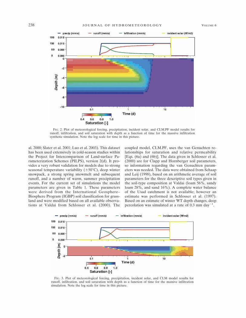
Figures 2 and 3 show plots of the results of this simu-lation for CLM.PF and CLM, respectively. Two keyforcing variables, precipitation and incident solar radia-tion, are plotted with runoff and infiltration, with theentire time series of the saturation profile plotted belowin each figure. In both plots, time is displayed on a logscale. Note the subsurface depth is 2 m in CLM and 10m in CLM.PF.

Infiltration starts almost immediately with the onsetof precipitation and initially represents a large fractionof the surface water balance. Inspection of Fig. 2 clearlyshows the infiltration response in CLM.PF on a loga-rithmic time scale, where a saturated infiltration frontadvances downward to the WT, shown in the figure asthe region of water saturation equal to 100% that formsat the ground surface and expands downward. As thesoil column fills with water, infiltration is moderatedand runoff increases. At approximately 5 days themodel has completely flooded and infiltration shuts off,and overland flow is the primary land surface flow pro-cess. Once the precipitation has ceased and incidentsolar radiation is turned on, the model slowly starts todry out and by the end of the simulation period (48days), the WT has slightly receded.

In Fig. 3 the very upper soil layer of CLM is seen torapidly saturate within a few hours, causing saturationexcess runoff to occur as a primary land surface flowprocess. The saturation front advances downward andreaches equilibrium within 10 days, but CLM does notflood. After the precipitation is turned off and incidentsolar radiation is imposed, CLM dries out, but muchmore rapidly than CLM.PF. Comparison of Figs. 2 and3 highlights some of the land surface hydrologic processdifferences between the CLM and coupled CLM.PFmodels. This demonstrates that the addition of a deepersoil column with an explicit representation of the WTand saturated zone has a pronounced effect on the re-sponse of water in the soil column.

b. Comparison with observations at UsadievskiyWatershed, Valdai, Russia

To provide a more realistic comparison of the CLMand CLM.PF models, an observed 18-yr meteorologicaldataset from the Usadievskiy Watershed (henceforthUsad) in Valdai, Russia, was used (Robock et al. 1995;Vinnikov et al. 1996; Schlosser et al. 1997; Schlosser et


al. 2000; Slater et al. 2001; Luo et al. 2003). This datasethas been used extensively in cold-season studies withinthe Project for Intercomparison of Land-surface Pa-rameterization Schemes (PILPS), version 2(d). It pro-vides a very robust validation for models due to strongseasonal temperature variability (�50°C), deep wintersnowpack, a strong spring snowmelt and subsequentrunoff, and a number of warm, summer precipitationevents. For the current set of simulations the modelparameters are given in Table 1. These parameterswere derived from the International Geosphere–Biosphere Program (IGBP) soil classification for grass-land and were modified based on all available observa-tions at Valdai from Schlosser et al. (2000). The

coupled model, CLM.PF, uses the van Genuchten re-lationships for saturation and relative permeability[Eqs. (6a) and (6b)]. The data given in Schlosser et al.(2000) are for Clapp and Hornberger soil parameters,so information regarding the van Genuchten param-eters was needed. The data were obtained from Schaapand Leij (1998), based on an arithmetic average of soilparameters for the three descriptive soil types given inthe soil-type composition at Valdai (loam 56%, sandyloam 28%, and sand 16%). A complete water balanceof the Usad catchment is not available; however anestimate was performed in Schlosser et al. (1997).Based on an estimate of winter WT depth changes, deeppercolation was simulated at a rate of 0.3 mm day�1.

FIG. 3. Plot of meteorological forcing, precipitation, incident solar, and CLM model results forrunoff, infiltration, and soil saturation with depth as a function of time for the massive infiltrationsimulation. Note the log scale for time in this picture.

FIG. 2. Plot of meteorological forcing, precipitation, incident solar, and CLM.PF model results forrunoff, infiltration, and soil saturation with depth as a function of time for the massive infiltrationsynthetic simulation. Note the log scale for time in this picture.


Fig 2 3 live 4/C

All of the observations at the Usad catchment weremade available by A. Robock and L. Luo as part of theGlobal Soil Moisture Databank (Robock et al. 2000;Luo et al. 2003), and all observations used for modelcomparisons come from these sources. Water table ob-servations are not commonly compared to LSM simu-lations. Typically, LSM simulations include a quantityof water in a lower soil layer that may vary in a similarmanner to WT depth (e.g., Fig. 10 of Schlosser et al.1997). It is for this reason that simulation of WT depthis one of the motivations of the current coupled modeland a focus of the results. The WT depth was recordedat many locations within the catchment (up to 20) andover a varying frequency, generally subweekly. Theseobservations were spatially averaged to provide acatchment average of WT depth and are presentedalong with the minimum and maximum WT depth inthe results below. Some of the more shallow wells werefrozen during portions of the winter. An indication thata well was frozen was provided in the original data.These wells were screened (as were wells for which WTmeasurements were not available) from the calculationof catchment-averaged WT depth during those periods.As there were a large number of wells in the watershed,and typically fewer than one or two wells for any givenmeasurement period were omitted, it was felt that thisdid not bias the results of the analysis.

There has been significant discussion (e.g., Yang etal. 1995) regarding the period of time a land surfacemodel takes to come into thermal and hydrologic equi-librium from an initial set of conditions (i.e., modelspinup). To insure proper model equilibrium a series ofback-to-back 18-yr model runs were performed withthe parameter values at the end of the first 18-yr simu-lation used as the initial condition for the second 18-yrsimulation. This not only provided for model equilib-rium but also provided information regarding modelspinup time, which was between 1.5 and 2 yr.

1) COUPLED MODEL, CLM.PF, RESULTS, ANDDISCUSSION

A portion of the results of the January 1966 to De-cember 1983 simulation are presented in three plots,each with a 3-yr time series (Figs. 4a–c, 1969–71, 1972–74, and 1981–83), where the following quantities arepresented:

(i) observed meteorological input forcing, daily aver-aged downward shortwave and longwave radia-tion, and reference temperature;

(ii) observed meteorological input forcing and monthlyand daily cumulative precipitation;

(iii) monthly averaged runoff observations and modelpredictions;

(iv) minimum, maximum, and averaged water table ob-servations plotted against daily averaged coupledmodel predictions;

(v) observations of snow water equivalent depth andmodel predictions; and

(vi) daily observations and model predictions of groundsurface temperature.

In general the model results agree with the observa-tions at the daily and monthly time scales (specific de-tails follow).

From visual inspection of Fig. 4, the monthly aver-aged CLM.PF runoff (RO) simulations agree well withthe timing and magnitude of the observations, with thebest agreement occurring during the spring snowmeltrunoff. The largest difference between the modeled andobserved snowmelt peak runoff is in April 1972 [Fig.4b(iii)]. Simulated daily averaged WT depth, SWE, andTs also agree well with observations. For all four sets ofsimulations, the coupled model replicates observeddaily variations and seasonal trends. Simulated WTdepth is a new coupled model predictive measure thatcaptures the summer variability and trends in observedWT depth. The WT depth observations are a site aver-age of the 19 observation wells, and in all cases themodel simulations fall within the minimum and maxi-mum observed depths. The majority of the discrepan-cies between model simulations and observation occurduring the winter months (e.g., December 1969 in Fig.4a). The topography of the watershed is such that sig-nificant lateral flow in the subsurface would be ex-pected. A one-dimensional column model cannot rep-licate this topography.

A suite of descriptive statistics was calculated for cor-responding pairs of simulations and observations intime and is presented in Table 2. Following the recom-mendations in Willmott (1982), the average values forthe observed and simulated (O, M) WT depth (meters),total monthly runoff (millimeters), SWE (millimeters),and Ts (degrees Celsius) along with the standard devia-tion of the observed and simulated values (so, sm), themean average error (MAE), the root-mean-square er-ror (rmse) and the systematic and unsystematic root-mean-square error (rmseS and rmseU), an index ofagreement (d), the slope of a least squares linear re-gression (m), the sample coefficient of determinationR2, and the number of comparison pairs (N). The val-ues listed for Table 2 are computed over the entire18-yr simulation period, while Table 3 displays a subsetof these comparison measures computed for eachmonth, for WT depth.

TABLE 1. List of model parameters used in Valdai simulation.

Parameter Value Units

� Van Genuchten alpha 1.95 (m�1)n Van Genuchten exponent 1.74Ksat Saturated hydraulic conductivity 1.21 (m day�1)� Effective soil porosity 0.401sres Residual saturation 0.136wfact Fraction of model area with

high WT0.15


Overall, the descriptive statistics presented in Table 2show agreement between model predictions and obser-vations. The 18-yr averaged, simulated WT depth, ROand SWE (M), overpredict the averaged observations(O), with WT overpredicting by 8% and RO and SWEoverpredicting by nearly 40%. On average, simulatedTs underpredicts the observations by 25%; Ts is theobservation most accurately predicted by CLM.PF,with the highest d and R2 values, while WT, RO, and

SWE are less accurately predicted by the model thanTs. The accuracy of predicted WT depth varies greatlyduring the year, as shown in Table 3. The statistics inTable 3 indicate that observed WT depth in May–November is much more accurately predicted byCLM.PF than December–April. Observed WT depthsduring the month of April are the least-accurately pre-dicted by the model. It should be noted that the spatialvariability in observed WT depth is always greater than

FIG. 4. (a) Plot of observed meteorological input forcing,CLM.PF model simulations, and corresponding observations forthe Usad catchment from Jan 1969 to Dec 1971. (i) and (ii) Theforcing; daily averaged downward shortwave and longwave radia-tion and temperature are depicted by black and gray curves andsymbols, respectively, in (i), and monthly and daily averaged pre-cipitation are depicted by the line with symbols and the gray line,respectively, in (ii). (iii) Monthly averaged runoff; (iv) daily mini-mum, average, and maximum WT depths; (v) snow water equiva-lent depth; and (vi) daily ground surface temperatures. (iii)–(vi)Observations plotted as symbols and CLM.PF model simulationsas solid curves. (b) Same as (a), but from Jan 1972 to Dec 1974. (c)Same as (a), but from Jan 1981 to Dec 1983.


the temporal variability in averaged WT depth over thecatchment (so � 0.9 m for spatial compared to so � 0.36for temporal).

Figure 5 presents a scattergram of daily observed andsimulated WT depth for the entire 18-yr simulation pe-riod. Visual inspection of this plot again indicates anoverall fair to good fit between observed and simulatedWT depths. The scattergram is broken out into threesubsets by Ts. The red dots, representing observed andsimulated WT measurements for Ts greater than 5°Cprovide the best fit, indicating that warm-weather pro-cesses are well represented by the coupled model. ForTs below �5°C, the coupled model tends to underpre-dict the observed WT depths and for the freeze–thawperiods (�5° to �5°C) the coupled model tends tooverpredict observed WT depths. These results agreewith the monthly statistics presented in Table 3.

As noted earlier, there is significant lateral subsur-face flow at the Usad site. This lateral flow has the mostsignificant effect on observed WT depths during thewinter months, when the ground surface is frozen, snowcovered, and hydraulically disconnected from the sub-surface. Surface processes other than topographywould have very little effect on the movement of theWT, and since infiltration and recharge are very lowduring the winter months the prime factor affecting wa-ter table levels would be redistribution due to gravity(e.g., Fig. 4b for January–February 1972). In this figure,temporal changes in average observed WT depth cor-respond with the minimum and maximum observed wa-ter table depth and the variability increases with time.The minimum observed water table depth is zero dur-ing this period, indicating discharge of groundwater at

the ground surface. The variability in observed summerWT depth (Fig. 4b, 1972) stays relatively constant overtime, and the fluctuations of the minimum, maximum,and average observed WT depth are in phase. Since thecoupled model is operating in a single-column mode, itcannot capture the lateral movement of the WT duringwinter months and a distributed (2D surface, 3D sub-surface) model would be needed to capture the varia-tions in water table depth during winter months.

The less accurate WT simulations during freeze–thaw(�5° to �5°C, inclusive) points to a different set ofprocesses. Inspection of the dates corresponding to thepoints of poorest estimation in Fig. 5 (e.g., the greendots, up and to the left of the 45° dashed line) indicatesthey occur during the spring snowmelt that generallyoccurs during the month of April. An example of ob-served WT depth during a corresponding spring snow-melt is shown in Fig. 6, which presents observed andsimulated runoff, WT depth, SWE, and Ts from Febru-ary 1966 to June 1966. Careful inspection of Fig. 6 in-dicates a slight lag in the simulated 1966 spring thawprocess. The simulated SWE is overestimated duringthis time, and there is a corresponding underestimationof the Ts as well. This underestimation of Ts and springsnowmelt causes the ground to remain frozen longerthan observations, delaying the infiltration front thatresults from spring snowmelt. This same set of pro-cesses may be seen during the 1981 spring melt period(Fig. 4c). This feature does not appear to be related tothe overestimation of midwinter SWE, as it is seen dur-ing the spring of 1966 (Fig. 6), which follows a winterwhere the SWE was not overestimated. This feature isnot seen in some spring thaws—spring 1983, for ex-

TABLE 3. Descriptive statistics of Usad observations (O) and model simulations (M ) of average WT depths aggregated by month.All quantities are in meters, except d and N, which are unitless.

Month O M so sm MAE Rmse RmseS RmseU d N

Jan 0.95 0.88 0.25 0.18 0.22 0.27 0.21 0.17 0.58 126Feb 1.11 0.92 0.21 0.17 0.23 0.30 0.25 0.16 0.53 104Mar 0.86 0.96 0.28 0.17 0.21 0.26 0.22 0.14 0.62 178Apr 0.54 0.79 0.19 0.14 0.26 0.32 0.29 0.14 0.50 495May 0.67 0.71 0.19 0.09 0.12 0.14 0.12 0.06 0.76 385Jun 0.97 0.92 0.29 0.17 0.15 0.18 0.15 0.09 0.85 181Jul 1.11 1.09 0.35 0.23 0.16 0.19 0.15 0.12 0.88 184Aug 1.19 1.16 0.37 0.25 0.16 0.20 0.16 0.12 0.89 165Sep 1.21 1.14 0.37 0.26 0.16 0.22 0.17 0.14 0.86 139Oct 0.82 0.92 0.36 0.25 0.19 0.24 0.19 0.14 0.84 174Nov 0.66 0.79 0.32 0.21 0.21 0.27 0.22 0.16 0.73 166Dec 0.72 0.83 0.26 0.22 0.24 0.32 0.24 0.21 0.52 154

TABLE 2. Descriptive statistics of Usad observations (O) and model simulations (M ). All quantities are in the units given (m, mm,and °C), except m, d, R2, and N, which are unitless.

O M so sm MAE Rmse RmseS RmseU d m R2 N

WT (m) 0.82 0.89 0.36 0.23 0.19 0.25 0.20 0.16 0.81 0.49 0.55 2451RO (mm) 23 32 40 43 22 32 13 29 0.84 0.67 0.52 205SWE (mm) 84 116 48 54 40 51 34 38 0.77 0.80 0.51 232Ts (°C) 4.2 3.2 12.0 13.5 2.5 3.3 1.6 2.9 0.98 1.09 0.95 6574


ample (Fig. 4c)—where the timing of snowmelt andground thaw agrees well with observations, resulting ingood agreement of the WT simulations and observations.

Figure 7 further explores the simulation of Ts via ascattergram of observed and simulated daily averagedTs, showing very good agreement between model simu-lations and observations, as also indicated by Table 2.There are some underestimations of daily averaged Ts

with a maximum underestimation of 25°C, detailed onthe figure by a dashed oval. Inspection of the dates ofthese underestimations reveals that they correspond tospring snowmelt and thaw periods, including the onesdiscussed above, primarily during the month of April.Comparison statistics similar to those presented for WTin Table 3 were also calculated for Ts. These statisticsshow CLM.PF did a poor job predicting observed Ts

during the month of April, with all indicators of modelperformance being much lower than other months (e.g.,99% error in average, d � 0.5, m � 0.35, and R2 � 0.28).

A further complication regarding the representationof cold processes in a 1D model is lateral spatial vari-ability. Luo et al. (2003) noted lateral variability in theform of fractional snow coverage at the Usad site. Thiswould lead to a different behavior than what is repre-sented in the single-column model, where snow is eitherpresent at some depth or absent altogether. The 1Dmodel is limited in its ability to represent situationswhere infiltration occurs at one location, due to snow-melt or rainfall, and not at other locations (where snowcompaction or other processes might be taking place).This further substantiates the need to understand theaffect of spatial variability on these processes.

2) COMPARISON OF THE COUPLED ANDUNCOUPLED MODELS, CLM.PF AND CLM,RESULTS AND DISCUSSION

Figure 8 presents a comparison of simulations forboth the coupled (CLM.PF) and uncoupled (CLM)models compared to the Usad observations. In this fig-ure, monthly averaged precipitation, runoff, sensibleheat flux, and evapotranspiration are plotted. Thesimulations of sensible heat flux and evapotranspirationfor the coupled and uncoupled models agree closely.The model simulations for runoff do include some dif-ferences, specifically during the periods of spring snow-melt. The timing of the spring snowmelt is similar forboth the coupled and uncoupled models. However, therunoff rates are more accurately simulated by thecoupled model, with the uncoupled model tending to

FIG. 5. Plot of observed vs simulated WT depth in meters. Thethree colors are separated out for ground surface temperaturesbelow –5°C (blue, m � 0.27, R2 � 0.37), from –5° to �5°C (green,m � 0.27, R2 � 0.28), and greater than �5°C (red, m � 0.64, R2

� 0.80).

FIG. 6. Plot of observed and simulated runoff, groundwaterdepth, snow water equivalent depth, and ground surface tempera-ture for the Usad catchment from Feb 1966 to Jun 1966. Obser-vations are plotted as symbols, and CLM.PF model simulationsare plotted as solid curves.


Fig 5 live 4/C

underestimate the observed flow rate. The similarity inthe two models’ simulations of evapotranspirationwould indicate a similarity in simulations of shallow soilmoisture profiles. The differences in runoff would indi-cate a difference in simulations of deeper soil moistureas well as the effect of the explicit simulation of WT,

something present in the coupled model but absent inthe uncoupled model.

Both the coupled and uncoupled models underpre-dict the evapotranspiration during summer months1966 to 1972 (Figs. 8a and 8b), with 1972–73 (Fig. 8b)providing the best agreement between simulations andmodel observations. This underprediction, though sig-nificant in some years, falls within the range of evapo-transpiration simulations reported by the PILPS 2(d)experiment. Figure 11a of Schlosser et al. (2000) plotsthe 21 model simulations to observed evapotranspira-tion at Usad. For example, the PILPS 2(d) model simu-lations range from 1.8 to 4.2 mm day�1 for June 1972and 1.9 to 4 mm day�1 for July 1972; the CLM andCLM.PF model simulations (presented in Fig. 8b) are2.7 mm day�1 for June 1973 and 3.3 mm day�1 for July1973, and are close to the median among the range ofmodel predictions.

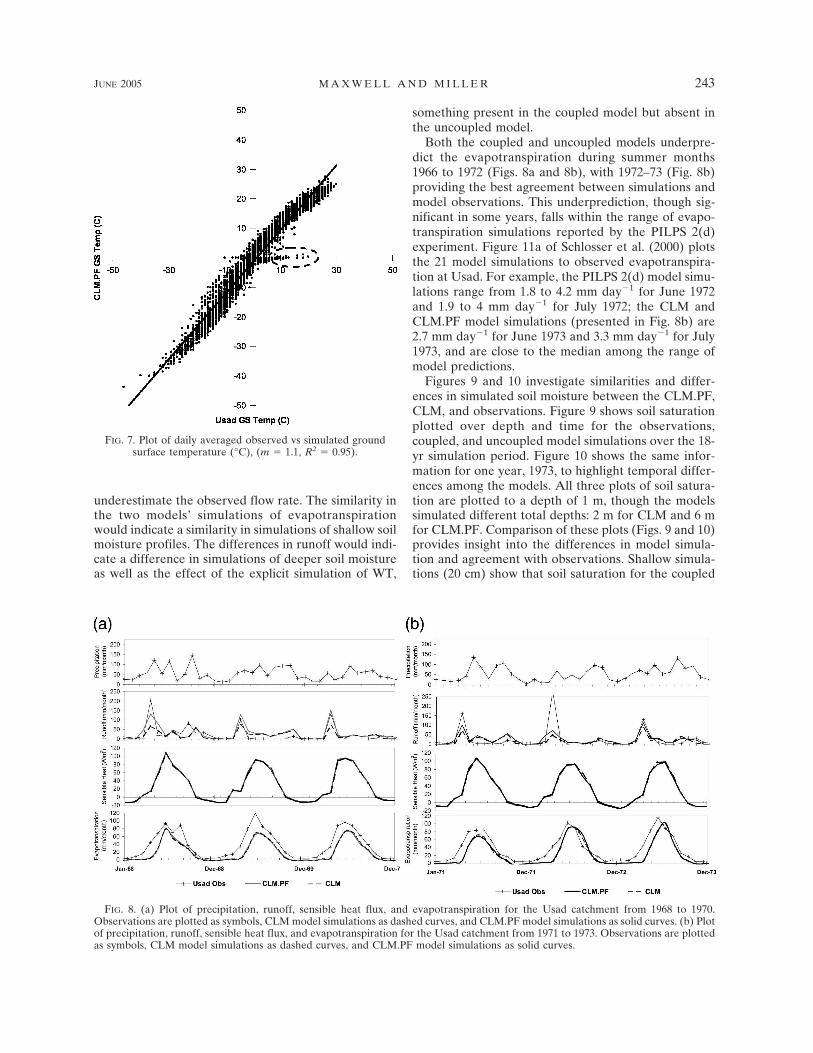
Figures 9 and 10 investigate similarities and differ-ences in simulated soil moisture between the CLM.PF,CLM, and observations. Figure 9 shows soil saturationplotted over depth and time for the observations,coupled, and uncoupled model simulations over the 18-yr simulation period. Figure 10 shows the same infor-mation for one year, 1973, to highlight temporal differ-ences among the models. All three plots of soil satura-tion are plotted to a depth of 1 m, though the modelssimulated different total depths: 2 m for CLM and 6 mfor CLM.PF. Comparison of these plots (Figs. 9 and 10)provides insight into the differences in model simula-tion and agreement with observations. Shallow simula-tions (20 cm) show that soil saturation for the coupled

FIG. 8. (a) Plot of precipitation, runoff, sensible heat flux, and evapotranspiration for the Usad catchment from 1968 to 1970.Observations are plotted as symbols, CLM model simulations as dashed curves, and CLM.PF model simulations as solid curves. (b) Plotof precipitation, runoff, sensible heat flux, and evapotranspiration for the Usad catchment from 1971 to 1973. Observations are plottedas symbols, CLM model simulations as dashed curves, and CLM.PF model simulations as solid curves.

FIG. 7. Plot of daily averaged observed vs simulated groundsurface temperature (°C), (m � 1.1, R2 � 0.95).


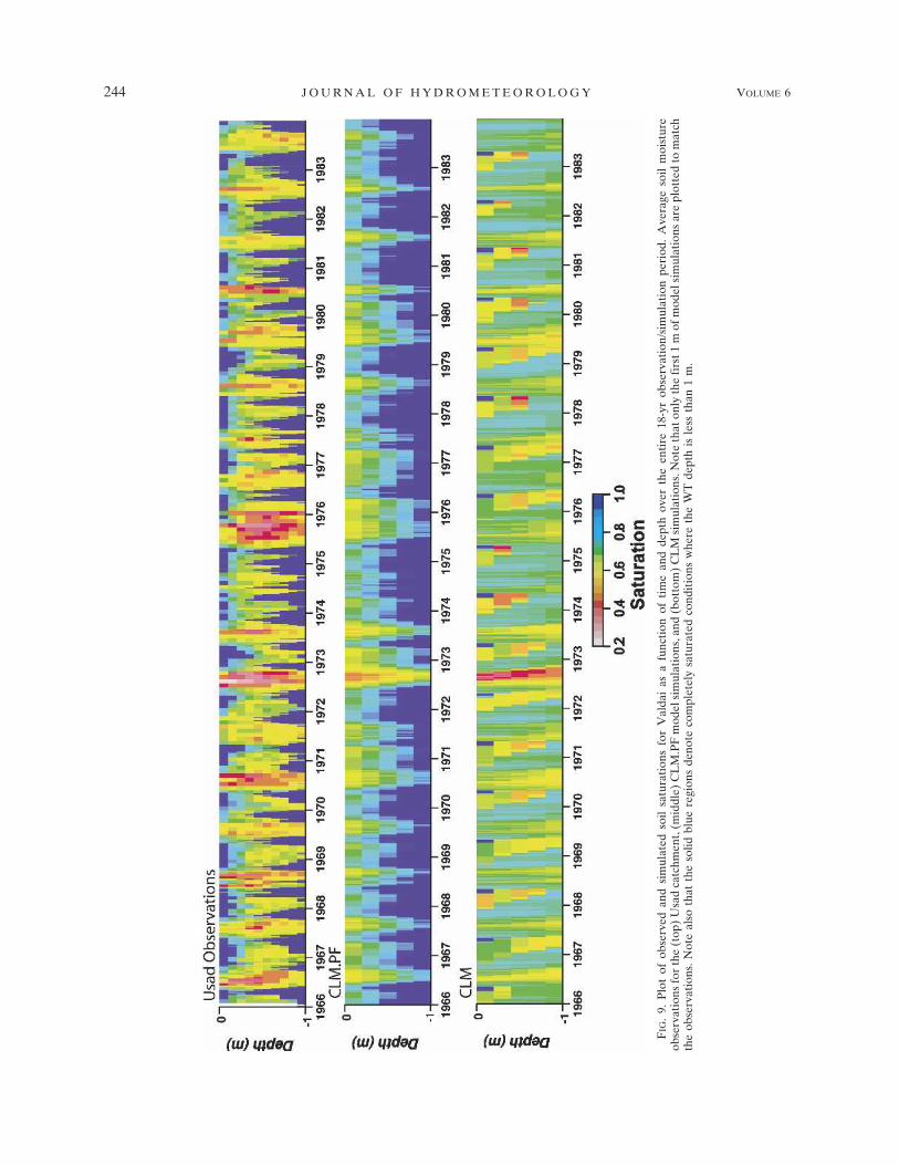
FIG

.9.

Plo

tof

obse

rved

and

sim

ulat

edso

ilsa

tura

tion

sfo

rV

alda

ias

afu

ncti

onof

tim

ean

dde

pth

over

the

enti

re18

-yr

obse

rvat

ion/

sim

ulat

ion

peri

od.

Ave

rage

soil

moi

stur

eob

serv

atio

nsfo

rth

e(t

op)

Usa

dca

tchm

ent,

(mid

dle)

CL

M.P

Fm

odel

sim

ulat

ions

,and

(bot

tom

)C

LM

sim

ulat

ions

.Not

eth

aton

lyth

efi

rst1

mof

mod

elsi

mul

atio

nsar

epl

otte

dto

mat

chth

eob

serv

atio

ns.N

ote

also

that

the

solid

blue

regi

ons

deno

teco

mpl

etel

ysa

tura

ted

cond

itio

nsw

here

the

WT

dept

his

less

than

1m

.


Fig 9 live 4/C

and uncoupled models are very similar, particularlyduring the summer months. This corresponds to thesimilarities in the simulated evapotranspiration be-tween the two models. Deeper simulations of soil satu-ration (40 cm and greater) are quite different betweenthe coupled and uncoupled models, with the coupledmodel simulations agreeing well with observations. TheCLM parameterization of the subsurface, including thesubsurface drainage and baseflow, is quite differentthan the parameterization used in CLM.PF. The un-coupled model also does not explicitly calculate a WTlocation, and these two factors contribute to differencesin simulated soil moisture below 40 cm and to differ-ences in simulated runoff and infiltration. CLM.PF storeswater in the subsurface, which has an effect on modelbehavior beyond seasonal time cycles. This effect canbe seen both in Figs. 8 and 9, where WT and soil mois-ture storage and memory affect other modeled processes.

4. Summary and conclusions

Coupling the land surface and groundwater modelsproduces a model, CLM.PF, that behaves much differ-

ently than the previously uncoupled land surface modeland expands the capabilities of the groundwater modelto include land surface processes. This coupled modelprovides simulations of the subsurface, which, becauseof the explicit accounting for water up to and below theWT, have a memory of water stored in the deep sub-surface. The simulations presented here show that thisscheme balances mass across the land surface/ground-water boundary and provides new insights into coupledprocesses. The coupled model yields different behaviorthan the uncoupled model under flooding conditions, asseen in section 3a. The coupled model also has a dif-ferent depiction of the root-zone soil moisture than theuncoupled model, leading to more realistic behaviorthat more closely matches observations at the Usad site[as discussed in section 3b(2)]. These differencesstem solely from the soil saturations calculated byParFlow and their impact on other calculated pro-cesses (e.g., runoff infiltration) in CLM.PF. The simu-lations of evapotranspiration are very similar betweenthe coupled and uncoupled models [section 3b(2)], butsimulations of runoff and soil moisture are improved inCLM.PF. The coupled model reproduces the averaged

FIG. 10. Plot of observed and simulated soil saturations for Valdai as a function of time and depth for 1973.Average soil moisture observations for the (top) Usad catchment, (middle) CLM.PF model simulations, and(bottom) CLM simulations. Note that only the first 1 m of model simulations are plotted to match the observations.Note also that the solid blue regions denote completely saturated conditions where the WT depth is less than 1 m.


Fig 10 live 4/C

observations for the Valdai wells [section 3b(1)], andsome discrepancies in WT during periods of freeze/thaw have been demonstrated. There are also diver-gences in simulation between the coupled model andthe Valdai data that warrant the need to investigate theaffects of representing some processes and parameters(such as topography, subsurface heterogeneity, runoff,infiltration, and snow) in a distributed manner. Param-eter uncertainty and spatial variability can be quite sig-nificant in surface and subsurface systems, and thoughit was not addressed in the current work and may affectoutcomes, it should be considered in future studies.Nevertheless, the coupled model demonstrates theneed for better groundwater representation in land sur-face schemes.

Acknowledgments. This work was conducted underthe auspices of the U.S. Department of Energy by theUniversity of California, Lawrence Livermore NationalLaboratory (LLNL), under Contract W-7405-Eng-48and Lawrence Berkeley National Laboratory (LBNL)under Contract DE-AC03-76F00098. This work wasfunded by DOE Fossil Energy Program NETL, NPTO,Tulsa, Oklahoma. The authors are indebted to A.Robock and L. Luo for the use of the Valdai data. Theauthors also wish to thank the three anonymous review-ers for adding to the clarity of this manuscript.

REFERENCES

Abromopoulos, F., C. Rosenzweig, and B. Choudhury, 1988: Im-proved ground hydrology calculations for global climatemodels (GCMs): Soil water movement and evaporation. J.Climate, 1, 921–941.

Ashby, S. F., and R. D. Falgout, 1996: A parallel multigrid pre-conditioned conjugate grandient algorithm for groundwaterflow simulations. Nucl. Sci. Eng., 124, 145–159.

Bonan, G. B., 1998: A Land Surface Model (LSM version 1.0) forecological, hydrological, and atmospheric studies: Technicaldescription and user’s guide. NCAR Tech. Note NCAR/TN-417�STR.

Clapp, R. B., and G. M. Hornberger, 1978: Empirical equationsfor some soil hydraulic properties. Water Resour. Res., 14,601–604.

Cosby, B. J., G. M. Hornberger, R. B. Clapp, and T. R. Ginn,1984: A statistical exploration of the relationships of soilmoisture characteristics to the physical properties of soils.Water Resour. Res., 20, 682–690.

Dai, Y. J., and Q.-C. Zeng, 1997: A land surface model (IA94) forclimate studies. Part I: Formulation and validation in of-lineexperiments. Adv. Atmos. Sci., 14, 433–460.

——, X. Zeng, and R. E. Dickinson, 2001: The Common LandModel (CLM): Technical documentation and user’s guide. 69pp.

——, and Coauthors, 2003: The Common Land Model. Bull.Amer. Meteor. Soc., 84, 1013–1023.

Dickinson, R. E., P. J. Kennedy, A. Henderson-Sellers, and M.Wilson, 1986: Biosphere–Atmosphere Transport Scheme(BATS) for the NCAR Community Climate Model. NCARTech. Note NCAR/TN-275�STR, 69 pp.

——, R. M. Errico, F. Giorgi, and G. T. Bates, 1989: A regionalclimate model for the western U.S. Climatic Change, 15, 383–422.

——, A. Henderson-Sellers, and P. J. Kennedy, 1993: Biosphere–

Atmosphere Transport Scheme (BATS) version le ascoupled to the NCAR Community Climate Model. NCARTech. Note NCAR/TN-387�STR, 72 pp.

Famiglieti, J. S., and E. F. Wood, 1991: Evapotranspiration andrunoff from large land areas: Land surface hydrology for at-mospheric general circulation models. Surv. Geophys., 12,179–204.

Foley, J. A., C. I. Prentice, N. Ramankutty, S. Lewis, D. Pollard,S. Sitch, and A. Haxeltine, 1996: An integrated biospheremodel of land surface processes, terrestrial carbon balance,and vegetation dynamics. Global Biogeochem. Cycles, 10,603–628.

Giorgi, F., 1990: Simulation of regional climate using a limitedarea model nested in a general circulation model. J. Climate,3, 941–963.

Jones, J. E., and C. S. Woodward, 2001: Newton-Krylov-multigridsolvers for large-scale, highly heterogeneous, variably satu-rated flow problems. Adv. Water Resour., 24, 763–774.

Liang, X., E. F. Wood, and D. P. Lettenmaier, 1994: A simplehydrolically-based model of land surface and energy fluxesfor general circulation models. J. Geophys. Res., 99, 14 415–14 428.

——, Z. Xie, and M. Huang, 2003: A new parameterization forsurface and groundwater interactions and its impact on waterbudgets with the variable infiltration capacity (VIC) landsurface model. J. Geophys. Res., 108, 8613, doi:10.1029/2002JD003090.

Manabe, S., J. Smagorinsky, and R. F. Strickler, 1965: Simulatedclimatology of a general circulation model with a hydrologiccycle. Mon. Wea. Rev., 93, 769–798.

Levine, J. B., and G. D. Salvucci, 1999: Equilibrium analysis ofgroundwater–vadose zone interactions and the resulting spa-tial distribution of hydrologic fluxes across a Canadian prai-rie. Water Resour. Res., 35, 1369–1383.

Luo, L., and Coauthors, 2003: Effects of frozen soil on soil tem-perature, spring infiltration, and runoff: Results from thePILPS 2(d) experiment at Valdai, Russia. J. Hydrometeor., 4,334–351.

Oleson, K. W., and Coauthors, 2004: Technical description of theCommunity Land Model (CLM), NCAR Tech. Note NCAR/TN-461�STR, 173 pp.

Pikul, M. F., R. L. Street, and I. Remson, 1974: A numericalmodel based on coupled one-dimensional Richards andBoussinesq equations. Water Resour. Res., 10, 295–302.

Richards, L. A., 1931: Capillary conduction of liquids through po-rous mediums. Physics, 1, 318–333.

Robock, A., K. Ya. Vinnikov, C. A. Schlosser, N. A. Speranskaya,and Y. Xue, 1995: Use of midlatitude soil moisture and me-teorological observations to validate soil moisture simula-tions with biosphere and bucket models. J. Climate, 8, 15–35.

——, K. Y. Vinnikov, G. Srinivasan, J. K. Entin, S. E. Hollinger,N. A. Speranskaya, S. Liu, and A. Namkhai, 2000: The Glob-al Soil Moisture Data Bank. Bull. Amer. Meteor. Soc., 81,1281–1299.

Russell, G., and J. Miller, 1990: Global river runoff calculatedfrom a global atmospheric general circuation model. J. Hy-drol., 117, 241–254.

Salvucci, G. D., and D. Entekhabi, 1995: Hillslope and climaticcontrols on hydrologic fluxes. Water Resour. Res., 31, 1725–1739.

Schaap, M. G., and F. J. Leij, 1998: Database-related accuracy anduncertainty of pedotransfer functions. Soil Sci., 163, 765–779.

Schlosser, C. A., A. Robock, K. Ya. Vinnikov, N. A. Speranskaya,and Y. Xue, 1997: 18-year land surface hydrology modelsimulations for a midlatitude grassland catchment in Valdai,Russia. Mon. Wea. Rev., 125, 3279–3296.

——, and Coauthors, and the PILPS 2(d) Contributors, 2000:Simulations of a boreal grassland hydrology at Valdai, Rus-sia, PILPS Phase 2(d). Mon. Wea. Rev., 128, 301–321.

Sellers, P. J., Y. Mintz, Y. C. Sud, and A. Dalcher, 1986: A simple


biosphere model (SiB) for use with general circulation mod-els. J. Atmos. Sci., 43, 505–531.

Slater, A. G., and Coauthors, 2001: The representation of snow inland surface schemes: Results from PILPS 2(d). J. Hydrom-eteor., 2, 7–25.

van Genuchten, M. Th., 1980: A closed form equation for pre-dicting the hydraulic conductivity of unsaturated soils. SoilSci. Soc. Amer. J., 44, 892–898.

Vinnikov, K. Ya., A. Robock, N. A. Speranskaya, and C. A.Schlosser, 1996: Scales of temporal and spatial variability ofmidlatitude soil moisture. J. Geophys. Res., 101, 7163–7174.

Walko, R. L., and Coauthors, 2000: Coupled atmosphere–biophysics–hydrology models for environmental modeling. J.Appl. Meteor., 39, 931–944.

Willmott, C. J., 1982: Some comments on the evaluation of modelperformance. Bull. Amer. Meteor. Soc., 63, 1309–1313.

Wood, E. F., D. P. Lettenmaier, and V. G. Zartarian, 1992: Aland-surface hydrology parameterization with subgrid vari-ability for general circulation models. J. Geophys. Res., 97(D3), 2717–2728.

Yang, Z.-L., R. E. Dickinson, A. Henderson-Sellers, and A. J.Pitman, 1995: Preliminary study of spin-up processes in landsurface models with the first stage of Project for Intercom-parison of Land Surface Parameterization Schemes Phase1(a). J. Geophys. Res., 100, 16 553–16 578.

Yeh, P. J.-F., and E. A. B. Eltahir, 2005: Representation of watertable dynamics in a land-surface scheme. Part I: Model de-velopment. J. Climate, 18, 1861–1880.


Development of a Coupled Land Surface and … of a Coupled Land Surface and Groundwater Model ... by...

Documents

Transcript of Development of a Coupled Land Surface and … of a Coupled Land Surface and Groundwater Model ... by...