Development of a Computable General Equilibrium (CGE) Model

for Fisheries*

Christos Floros + and Pierre Failler + Author for correspondence Centre for the Economics and Management of Aquatic Resources, University of Portsmouth, Boathouse No. 6, College Road, H.M. Naval Base, Portsmouth, PO1 3LJ, UK. E-Mail: Christos.Floros@port.ac.uk, Tel: +44 (0) 2392 844244. APRIL 2004

Abstract This paper gives an introduction to Computable General Equilibrium (CGE) modelling, and presents an application of the technique to fisheries using data from Salerno, Italy. First, this study explains the data requirements for CGE model of the type employed. Second, we explain the process that can be used to develop and employ an applied static CGE model. Then we use the model for policy analysis. The main purpose of this paper is to contribute to and facilitate the use of general equilibrium models for policy and decision-making by looking at the relationship between economics and biology. To the best of our knowledge, this is the first application of a CGE model applied to fishing industry. Our model offers some interesting conclusions that help us to better understand the modelling and dynamics of fisheries (and in particular the link between economy-biology) when considered as a whole sector in interaction with the rest of the economy. * Part of the EU funded RTD project QLRT-2000-02277 “PECHDEV”. Keywords: Fisheries, SAM, Computable General Equilibrium Model, Salerno.

I. INTRODUCTION

General equilibrium (GE) theory suggests that real-world markets are

interdependent where changes in supply or demand conditions usually have

repercussions on supply and demand conditions. Since the beginning of the 1980s GE

models have become popular to analyse and describe economy, because they provide

quantitative results in policy analysis. General equilibrium models are increasingly

being used for many problems (see Harberger, 1962; Shoven and Whalley, 1992).

They may be applied to any large economic change. Computable general equilibrium

(CGE) model is a policy model where the main goal is to formulate a model of

simultaneous equilibrium1.

In this paper, we focus on a static CGE model. We give a brief introduction to

CGE modelling, and we provide a simple basic structure that can be used for the

development of a CGE model for fisheries. The main goal of this study is to develop a

CGE model for the evaluation of the socio-economic contributions of the fishing

activities. From fishery management point of view, it is necessary to employ a

regional economic model and estimate the regional economic impacts attributable to

fishery policies. For our simple example we consider real data from Salerno, Italy.

Our regional model is the first CGE model applied to fisheries, where the link

between economics and biology is presented.

The paper is organised as follows: Section II provides the data (SAM) from

Salerno-Italy, while Section III presents the general structure of a CGE model.

Section IV presents the CGE model statement, while in Section V we discuss the

application of a CGE model to fisheries. Section VI presents the main empirical

results for Salerno obtained using GAMS2 software package (www.gams.com).

Finally, Section VII concludes the paper and proposes future research.

1 The simplest form of general equilibrium model is the input-output model developed by Leontief. 2 GAMS (General Algebraic Modelling System) is an optimisation software. Other software package similar to GAMS is GEMPACK.

II. THE SOCIAL ACCOUNTING MATRIX

CGE modelling takes the following steps: (i) database construction, (ii) model

estimation and calibration, (iii) base run solutions and (iv) simulations, i.e. solving the

model under different scenarios (for CGE steps see Appendix 3).

First, a CGE model is usually based on a Social Accounting Matrix (SAM)

database, which is an extension of the I-O matrix. A SAM is a matrix of balanced

expenditure and income accounts. In the SAM, the column entries represent

expenditures to payments made by economic agents, while the row entries represent

receipts of income to agents. All receipts are equal to all expenditures, in the form that

the matrix gives a record of interrelationships in an economy at the level of individual

production sectors and factors, as well as private, public and foreign institutions.

Our SAM distinguishes the following accounts: activities, commodities, factors,

households, savings, taxes and the rest of the world. Activity column entries indicate

expenditures incurred during the production process and include purchases of

intermediate inputs and payments to the factors of production. The total supply of

commodities, value at market prices, is given as domestic marketed production,

imports of goods and non-factor services, indirect taxes as well as export taxes. The

commodity row gives the total demand for marketed commodities and includes

household and government consumption. The intersection between the commodity

column and government row gives the indirect taxes paid. Furthermore, factors

include labour and capital. The factor account pays factor taxes to the government and

factor payments to the RoW. Household column indicates the allocation of total

household income among income taxes and savings.

In addition, the savings-investment column gives the total investment expenditure in

the economy, while the RoW column shows the exports of goods and services.

Purchases of imports and receipts of factor payments are specified in the row.

In general, the SAM provides a snapshot of the economy at a single point in time

and each cell records the value of each transaction (i.e. the product of prices and

quantities).

Appendix 1 shows an example of a SAM structure used in a general CGE model.

III. OVERVIEW OF THE STATIC CGE MODEL

- CGE General Structure

In this section we present the general structure of a static CGE model. The main

characteristic of static CGE models is that data for modelling are either I-O tables

and/or national accounts for a single year.

In general equilibrium theory we formulate a model of simultaneous equilibrium in

competitive markets for all commodities. The model explains all payments based on

the SAM. In the standard CGE models, one first distinguishes between different

producers, goods and factors. According to the theory, producers maximise profits,

while consumers maximise utility. In this type of model, equilibrium is then

characterised by a set of prices and levels of production (i.e. market demand equals

supply for all commodities). The model is based on a system of simultaneous

equations, in which factors are fully utilized (see Dervis, de Melo and Robinson,

1982; Robinson, 1990 for more details). Prices are set so that equilibrium profits of

firms are zero. Factor incomes are divided among households (total household income

is used to pay taxes, save and consume), while government revenue comes from direct

and indirect taxes. Household incomes equal household expenditures (equilibrium

condition). Household goods consumption is determined by assumptions about

consumer behaviour. Consumers are generally assumed to maximize utility, where the

assumed form of the utility is a CES, a Linear expenditure system or a Translog

function. Furthermore, government tax revenues equal government expenditures

including subsidy payments. The Rest of the World supplies imports and demands

export goods. This section gives an overview of the basic CGE model by explaining

all the payments that are recorded in our SAM.

CGE models are based on the Walrasian general equilibrium structure (Walras,

1954). Accordingly, “for any price vector, the value of the excess demand is

identically zero”. For production, we have two types: Cobb-Douglas (CD) and

Constant Elasticity of substitution (CES). If the production function has no constant

returns of scale, we can calculate the different supply functions. The model satisfies

Walras law in that the set of commodity market equilibrium conditions is functionally

dependent.

In most CGE models, imports are determined by an import demand function. CGE

models employ the “Armington assumption” that products produced in different

regions are different from each other in quality (Armington, 1969). Armington has

three advantages: (i) it accounts for the large amount of cross-hauling present in the

data (imports and exports), (ii) it explains the empirical observation clear, and (iii) it

allows for differing degrees of substitution among different products and goods.

Furthermore, exports of a good depend on the ratio of the domestic price of the good

and the export price of the good. There is a distinction between domestically supplied

goods and exported goods according to a constant elasticity of transformation (CET)

function.

To run a CGE model, we estimate a number of parameters from the model, so that

the equilibrium solution satisfies all our equations under the method of “calibration”.

Because CGE models contain so many parameters to be estimated, the only way is to

use the estimation method called calibration. Calibration for CGE models can be used

in order to estimate parameters in, for example, Cobb-Douglas, CES and CET

functions. In addition, we need information of prices, quantities and values in the

initial equilibrium for model estimation. For instance, we can set all the prices at unity

at the initial equilibrium condition (homogeneity of degree zero). Figure 1 presents

the structure of a production technology when specified by a CES. Figure 2 shows the

structure of a simple model of one country, 2 producing sectors and 3 goods (imports,

M; domestic production, D; and exports, E). For general CGE steps see Appendix 3.

Figure 1. Production technology

Commodity Outputs

Activity CES/Leontief

Value added CES

Primary factors

Intermediate Leontief

Composite commodities

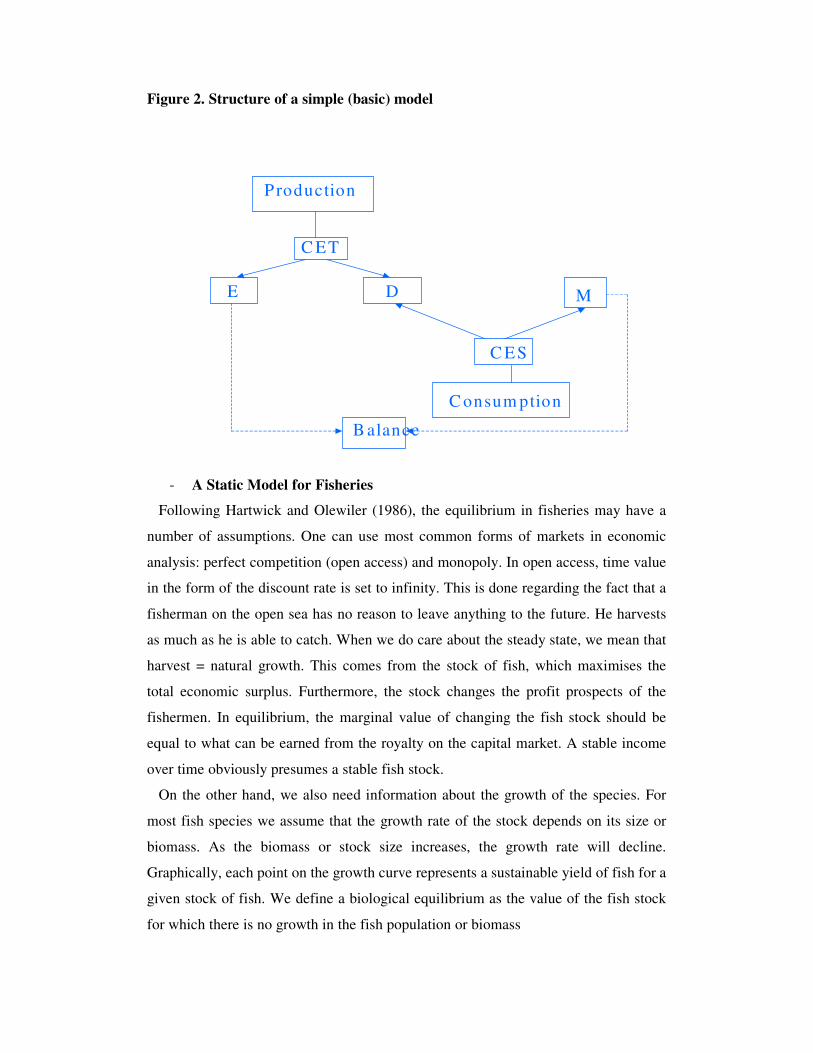
Figure 2. Structure of a simple (basic) model

- A Static Model for Fisheries

Following Hartwick and Olewiler (1986), the equilibrium in fisheries may have a

number of assumptions. One can use most common forms of markets in economic

analysis: perfect competition (open access) and monopoly. In open access, time value

in the form of the discount rate is set to infinity. This is done regarding the fact that a

fisherman on the open sea has no reason to leave anything to the future. He harvests

as much as he is able to catch. When we do care about the steady state, we mean that

harvest = natural growth. This comes from the stock of fish, which maximises the

total economic surplus. Furthermore, the stock changes the profit prospects of the

fishermen. In equilibrium, the marginal value of changing the fish stock should be

equal to what can be earned from the royalty on the capital market. A stable income

over time obviously presumes a stable fish stock.

On the other hand, we also need information about the growth of the species. For

most fish species we assume that the growth rate of the stock depends on its size or

biomass. As the biomass or stock size increases, the growth rate will decline.

Graphically, each point on the growth curve represents a sustainable yield of fish for a

given stock of fish. We define a biological equilibrium as the value of the fish stock

for which there is no growth in the fish population or biomass

Production

C onsum ption

E D M

B alance

C ET

C ES

IV. CGE MODEL STATEMENT

In this section we present the variables and equations for a static CGE model

(Lofgren et al., 2001). A static CGE model does not deal with issues of next periods.

The variables are divided into four parts: prices, production, institutions and system

constraints (see Table 1). The equations (mathematical statement of the model) are

presented in more details in Appendix 4.

Table 1. CGE Variables and Equations

VARIABLES EQUATIONS

Import price = tariff adjustment*exchange rate*import price

Export price = tariff adjustment * exchange rate * export price

Absorption =(domestic sales price*domestic sales

quantity)+(import price*import quantity)*(sales tax

adjustment)

Domestic Output Value (producer price*domestic output quantity) =

(domestic sales price*domestic sales quantity) +

(export price*export quantity)

Activity Price = (producer prices) * yields

Value-added Price = (activity price) – (input cost per activity unit)

Activity Production Funct. = f (factor inputs)

Factor Demand (Marginal cost of factor f in activity a) = (marginal

revenue product of factor f in activity a)

Intermediate demand = f (activity level)

Output function Domestic output = f (activity level)

Armington Function Composite supply = f (import quantity, domestic use

of domestic output)

Import-Domestic Demand

Ratio

= f (domestic-import price ratio)

Composite supply for

nonimported commodities

= domestic use of domestic output

CET Function Domestic output = f (export quantity, domestic use of

domestic output)

Export-Domestic Supply

Ratio

= f (export-domestic price ratio)

Output Transformation for

NonexportedCommodities

Domestic Output = domestic sales of domestic output

Factor Income Household factor income = (income share to

household h)* (factor income)

Household income = (factor incomes) + (transfers from government)

*ROW

Household Consumption

Demand for commodity c

= f (household income, composite price)

Investment Demand for

commodity c

= (base-year investment) * (adjustment factor)

Government Revenue = (direct taxes) + (transfers from ROW)+ (sales tax) +

(import tariffs) + (export taxes)

Government Expenditures (Government spending) = (household transfers) +

(government consumption)

Factor Markets (Demand for factor f) = (supply of factor f)

Composite Commodity

Markets

(Composite supply) = (composite demand, sum of

intermediate, household, government, investment

demand)

Savings-Investment Balance (Household savings) +(government savings)+(foreign

savings)=(investment spending)+(WALRAS dummy

variable)

V. CGE MODEL FOR FISHERIES

Applied literature focusing on general equilibrium effect on fisheries is small.

However, many previous studies of regional economic impacts of fishery used Input-

Output (I-O) models. We have three main categories in the literature: commercial

fishing, sport fishing and those that deals with both. Studies in the first category

include King and Shellhammer (1981) and Butcher et al. (1981). Furthermore, Martin

(1987) and Hammel et al. (2002) explain sport fishing, while Hushak et al. (1986) and

Carter and Radtke (1986) show the impact of fishery dealing with the third category.

Computable General Equilibrium (CGE) Models for Fisheries is not a widely area

of research. With an applied CGE model we can take into account the fish population

dynamics. To our knowledge, only one CGE model of this type exists, the recent

study of Houston et al. (1997). They develop a regional CGE model to evaluate the

impacts associated with reduced marine harvests for a coastal Oregon region. They

use five fishing sectors or vessel types, groundfish trawlers, crabbers, shrimp and

scallop draggers, whiting midwater trawlers and small boats. The Oregon model has

five processing sectors, 24 aggregated industry and commodity sectors, household

income categories, two government expenditures, three factor income accounts and an

investment expenditure account. Appendix 2 shows an example of a SAM structure

for fisheries used in and proposed by Houshak et al. (1997).

Houston et al. (1997) present three scenarios for Oregon CGE model. According to

the first scenario, there is a 20% reduction in groundfish catch because the fishery has

become less productive and/or more restrictive. Under this scenario, boats catch less

per unit fishing effort. Under the second scenario, there is a $6 million buyback of 16

trawl boats. It is assumed that this money comes from the federal government, or

some other source outside the local economy. Finally, the third scenario assumes a

removal of 16 trawl boats. Under the three policy scenarios, Houston et al. (1997)

estimate changes in numbers of jobs (i.e. employment impacts of reduced groundfish

harvests). The results show a bigger change (effect) on scenario 1.

Our model is different than that of Houston et al. (1997) because we are looking at

the linkage between biology and economics. Next we present the static CGE model

for Salerno (Salerno-CGE model).

VI. THE SALERNO-CGE MODEL & RESULTS

The Computable general equilibrium model for Salerno is a static model of the

Salerno economy calibrated to 2001 (for obvious reasons we can’t present the full

Salerno-SAM here). The structure of the Salerno CGE model is as follows: the

Salerno-CGE model is disaggregated into two Households (fisheries and non-

fisheries), two Factors (labor and capital), two Firms, 29 Activities, 37 Commodities,

Government, 6 Taxes, Savings and the Rest-of-the-World (RoW).

Our regional model has two components: a CGE model, which represents the

behaviour of economic agents (i.e. economic part), and a biology model, which is a

representation of biological process affecting fisheries productivity (under the

biological production functions for Salerno).

The economic part of CGE model for Salerno employs standard assumptions. The

model assumes that producers maximize profits subject to production functions, while

households maximize utility subject to budget constraints. Production and

consumption behaviour are modelled using the constant elasticity of substitution

(CES) family of functions, which includes Leontief3, Cobb-Douglas and constant

elasticity of transformation (CET) functions. Hence, substitution between regional

supply and exports is given by CET, while firms smoothly substitute over primary

factors through CES functions. Furthermore, factors are mobile across activities,

available in fixed supplies, and demanded by producers at market-clearing prices. The

model satisfies Walras’ law in that the set of commodity market equilibrium

conditions is functionally dependent, while the model is homogeneous of degree of

zero in prices. Other main assumptions are the following two: first, the Salerno is

treated as an open economy, implying that Salerno faces exogenous prices for imports

and exports. Second, products are differentiated according to region and Armington

assumption, so that imports and exports are different from domestically produced

goods.

Regarding the Savings, its row receives payments from the household, while its

column shows spending on commodities for investment. We assume that (i)

household income is allocated in fixed shares to savings and consumption, (ii) the

value of total investment spending is determined by the value of savings and (iii)

investment spending is allocated by the commodities. Here, the set of equilibrium

conditions includes the commodity market equilibrium conditions as well as the

savings-investment balance (including the Walras variable). Note that if the CGE

model works, then Walras should be zero. Furthermore, the government of the model

earns its revenues from income and sales taxes and spends it on consumption and

transfers to households. Government savings is the difference between its revenues

and spending. The income tax is a fixed share of the gross income of each

household.sales taxes are fixed shares of producer commodity prices. The government

consumes commodity quantities, and pays market prices and taxes. The final account

of our model is the rest of the world (RoW).

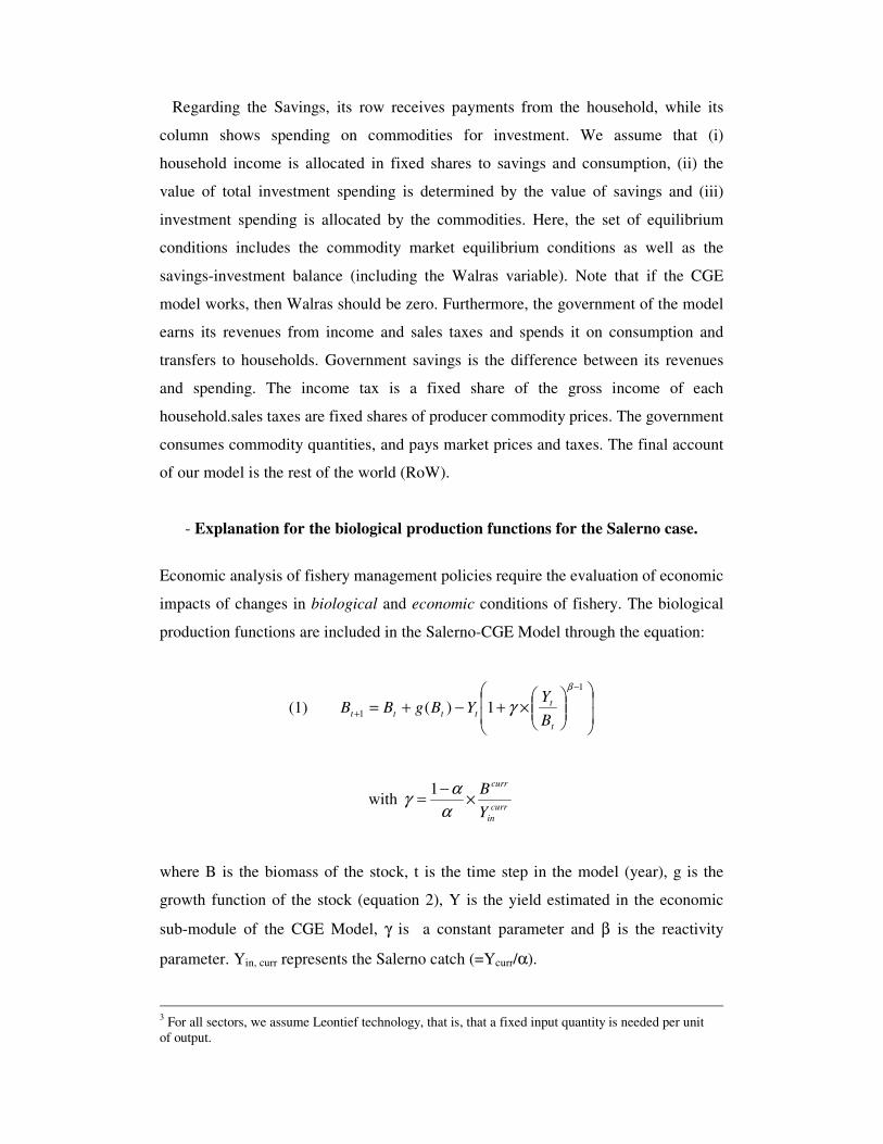
- Explanation for the biological production functions for the Salerno case.

Economic analysis of fishery management policies require the evaluation of economic

impacts of changes in biological and economic conditions of fishery. The biological

production functions are included in the Salerno-CGE Model through the equation:

(1) ��

�

�

��

�

�

���

����

�×+−+=

−

+

1

1 1)(β

γt

ttttt B

YYBgBB

with curr

in

curr

YB×−=

ααγ 1

where B is the biomass of the stock, t is the time step in the model (year), g is the

growth function of the stock (equation 2), Y is the yield estimated in the economic

sub-module of the CGE Model, γ is a constant parameter and β is the reactivity

parameter. Yin, curr represents the Salerno catch (=Ycurr/α).

3 For all sectors, we assume Leontief technology, that is, that a fixed input quantity is needed per unit of output.

Growth function

For the Salerno case, the biologic functions of growth g(B) can either be in the form

of a Pella and Tomlinson (generalized production model) with 3 parameters r, K, m,

either in the form of a Fox model (exponential model) with only 2 parameters. In this

case, the parameter value of m is one but the equation is different. All the stocks with

a m value of one in table I follow a Fox model whereas the others follow a Pella and

Tomlinson model.

The growth in the Fox model:

(2) ��

���

�××=BK

BrBg ln)(

The growth in the Pella and Tomlinson model:

(3) ��

�

�

��

�

���

���

�−=−1

1)(m

KB

BrBg

Values of reactivity β

Two values of β can be first tested in the Salerno case:

- β=1 corresponds to the fact that a variation in the fishing effort of the Salerno

fleet (increase for instance) will be followed by the same reaction of the other

fleets targeting the same stock (increase). This assumes that the biological

production function of Salerno matches exactly the production function of the

whole stock but only represents the relative part a of the fishing mortality (and

yield).

- β=0 corresponds to the situation in which the fishing effort of other fleets

applied on a given stock remain constant, whatever the variations of effort of

Salerno (assumption often made in bio-economic models).

To solve equation (1) we assume that ε<−+ tt BB 1 (=0.0001). So, we get that

)1(()()(1

1

−

+ ���

����

�×++−=

β

γt

ttttt B

YYBBBg

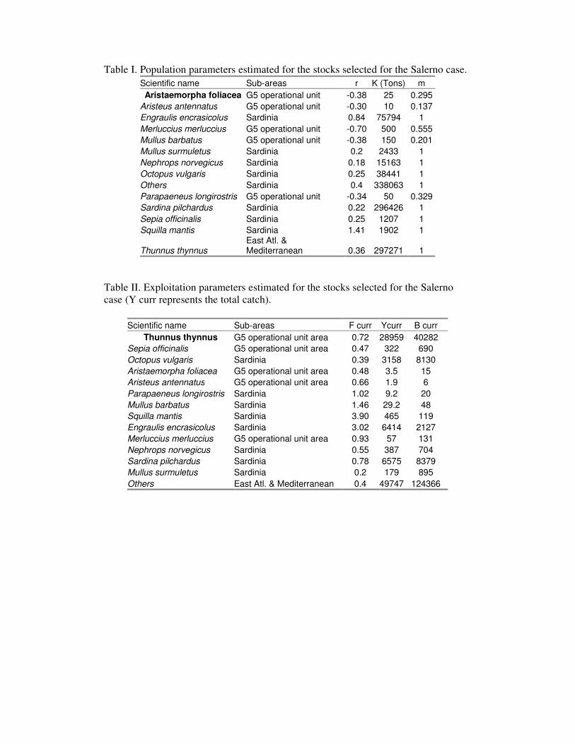
Table I. Population parameters estimated for the stocks selected for the Salerno case. Scientific name Sub-areas r K (Tons) m Aristaemorpha foliacea G5 operational unit -0.38 25 0.295

Aristeus antennatus G5 operational unit -0.30 10 0.137 Engraulis encrasicolus Sardinia 0.84 75794 1 Merluccius merluccius G5 operational unit -0.70 500 0.555 Mullus barbatus G5 operational unit -0.38 150 0.201 Mullus surmuletus Sardinia 0.2 2433 1 Nephrops norvegicus Sardinia 0.18 15163 1 Octopus vulgaris Sardinia 0.25 38441 1 Others Sardinia 0.4 338063 1 Parapaeneus longirostris G5 operational unit -0.34 50 0.329 Sardina pilchardus Sardinia 0.22 296426 1 Sepia officinalis Sardinia 0.25 1207 1 Squilla mantis Sardinia 1.41 1902 1

Thunnus thynnus East Atl. & Mediterranean 0.36 297271 1

Table II. Exploitation parameters estimated for the stocks selected for the Salerno case (Y curr represents the total catch).

Scientific name Sub-areas F curr Ycurr B curr Thunnus thynnus G5 operational unit area 0.72 28959 40282

Sepia officinalis G5 operational unit area 0.47 322 690 Octopus vulgaris Sardinia 0.39 3158 8130 Aristaemorpha foliacea G5 operational unit area 0.48 3.5 15 Aristeus antennatus G5 operational unit area 0.66 1.9 6 Parapaeneus longirostris Sardinia 1.02 9.2 20 Mullus barbatus Sardinia 1.46 29.2 48 Squilla mantis Sardinia 3.90 465 119 Engraulis encrasicolus Sardinia 3.02 6414 2127 Merluccius merluccius G5 operational unit area 0.93 57 131 Nephrops norvegicus Sardinia 0.55 387 704 Sardina pilchardus Sardinia 0.78 6575 8379 Mullus surmuletus Sardinia 0.2 179 895 Others East Atl. & Mediterranean 0.4 49747 124366

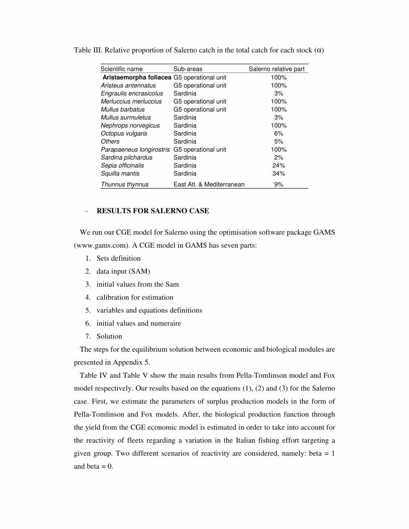
Table III. Relative proportion of Salerno catch in the total catch for each stock (α)

- RESULTS FOR SALERNO CASE

We run our CGE model for Salerno using the optimisation software package GAMS

(www.gams.com). A CGE model in GAMS has seven parts:

1. Sets definition

2. data input (SAM)

3. initial values from the Sam

4. calibration for estimation

5. variables and equations definitions

6. initial values and numeraire

7. Solution

The steps for the equilibrium solution between economic and biological modules are

presented in Appendix 5.

Table IV and Table V show the main results from Pella-Tomlinson model and Fox

model respectively. Our results based on the equations (1), (2) and (3) for the Salerno

case. First, we estimate the parameters of surplus production models in the form of

Pella-Tomlinson and Fox models. After, the biological production function through

the yield from the CGE economic model is estimated in order to take into account for

the reactivity of fleets regarding a variation in the Italian fishing effort targeting a

given group. Two different scenarios of reactivity are considered, namely: beta = 1

and beta = 0.

Scientific name Sub-areas Salerno relative part Aristaemorpha foliacea G5 operational unit 100%

Aristeus antennatus G5 operational unit 100% Engraulis encrasicolus Sardinia 3% Merluccius merluccius G5 operational unit 100% Mullus barbatus G5 operational unit 100% Mullus surmuletus Sardinia 3% Nephrops norvegicus Sardinia 100% Octopus vulgaris Sardinia 6% Others Sardinia 5% Parapaeneus longirostris G5 operational unit 100% Sardina pilchardus Sardinia 2% Sepia officinalis Sardinia 24% Squilla mantis Sardinia 34%

Thunnus thynnus East Atl. & Mediterranean 9%

TABLE IV. Pella-Tomlinson model for Salerno case Yield 382 64 882 147Scientific Name Aristeus antennatus Merluccius Mullus barbatus Parapaeneus longirostrisSAM name Blue & Red shrimp Europ. Hake Stripped Mullet Deepwater Rose shrimpCGE name gsb-c eh-c sm-c drs-c R -0.3 -0.7 -0.38 -0.34K 10 500 150 50M 0.137 0.555 0.201 0.329B 6 131 48 20g 0.9972287 74.72757 27.09253 5.77554Alpha 1 1 1 1Ycurr 1.9 57 29.2 9.2Yin,curr 1.9 57 29.2 9.2Gama 0 0 0 0B(t+1) -375.00277 141.7276 -806.907 -121.224M*F 0.09042 0.51615 0.29346 0.33558 TABLE V. Fox model for Salerno case

Yield 637 39 456 745 11923 68 745 172 19287Scient. nameEngraulis Mullus sur Nephrops Octopus Others Sardina Sepia offic Squilla mant ThunnusSAM name Eur. AnchovyRed mulletNorw. Lobster Com. Octopus Others Eur. PilchardCom. CuttlefishSpottail Man Norw. Bluefin tunaCGE name an-c rm-c nl-c co-c os-c ep-c cc-c sms-c bt-cr 0.84 0.2 0.18 0.25 0.4 0.22 0.25 1.41 0.36K 75794 2433 15163 38441 338063 296426 1207 1902 297271m 1 1 1 1 1 1 1 1 1B 2127 895 704 8130 124366 8379 690 119 40282g 6384.35543 179.0101 389.0095131 3157.618169 49746.57 6573.6203 96.4622801 465.036319 28984.76alpha 0.03 0.03 1 0.06 0.05 0.02 0.24 0.34 0.09Ycurr 6414 179 387 3158 49747 6575 322 465 28959Yin,curr 213800 5966.667 387 52633.33333 994940 328750 1341.66667 1367.64706 321766.7gama 0.32166978 4.85 0 2.419949335 2.374971 1.2488852 1.62857143 0.16890323 1.265811Bt+1/beta=0 7190.164 -3305.74 637.0095 -9131.57 -133176 4420.211 -1082.25 391.9368 -1009.64Bt+1/beta=1 7669.452 845.8601 637.0095 8739.756 133872.8 14799.7 -1171.82 382.985 25566.06g(bt)/beta=0 704.9 984.8 456.0 5386.3 82714.1 176.2 3344.9 179.4 53246.5g(Bt)/beta=1 841.9 228.2 456.0 2547.9 40239.8 152.9 1958.3 201.1 43700.7

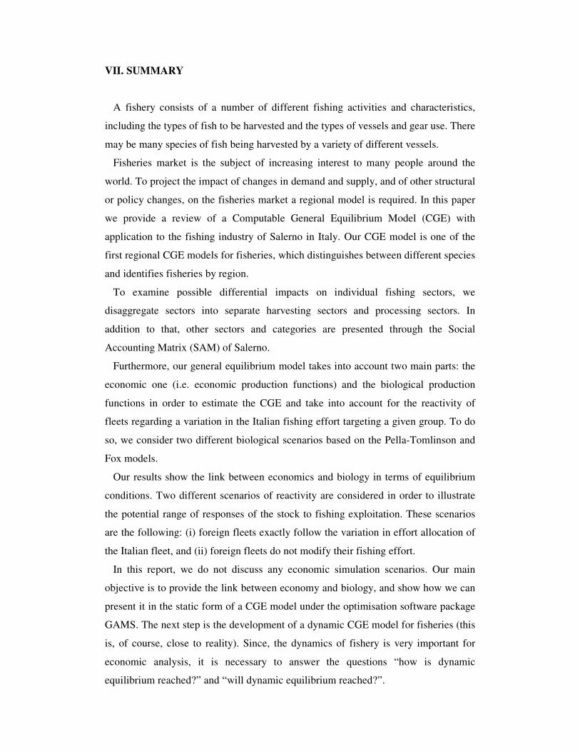
VII. SUMMARY

A fishery consists of a number of different fishing activities and characteristics,

including the types of fish to be harvested and the types of vessels and gear use. There

may be many species of fish being harvested by a variety of different vessels.

Fisheries market is the subject of increasing interest to many people around the

world. To project the impact of changes in demand and supply, and of other structural

or policy changes, on the fisheries market a regional model is required. In this paper

we provide a review of a Computable General Equilibrium Model (CGE) with

application to the fishing industry of Salerno in Italy. Our CGE model is one of the

first regional CGE models for fisheries, which distinguishes between different species

and identifies fisheries by region.

To examine possible differential impacts on individual fishing sectors, we

disaggregate sectors into separate harvesting sectors and processing sectors. In

addition to that, other sectors and categories are presented through the Social

Accounting Matrix (SAM) of Salerno.

Furthermore, our general equilibrium model takes into account two main parts: the

economic one (i.e. economic production functions) and the biological production

functions in order to estimate the CGE and take into account for the reactivity of

fleets regarding a variation in the Italian fishing effort targeting a given group. To do

so, we consider two different biological scenarios based on the Pella-Tomlinson and

Fox models.

Our results show the link between economics and biology in terms of equilibrium

conditions. Two different scenarios of reactivity are considered in order to illustrate

the potential range of responses of the stock to fishing exploitation. These scenarios

are the following: (i) foreign fleets exactly follow the variation in effort allocation of

the Italian fleet, and (ii) foreign fleets do not modify their fishing effort.

In this report, we do not discuss any economic simulation scenarios. Our main

objective is to provide the link between economy and biology, and show how we can

present it in the static form of a CGE model under the optimisation software package

GAMS. The next step is the development of a dynamic CGE model for fisheries (this

is, of course, close to reality). Since, the dynamics of fishery is very important for

economic analysis, it is necessary to answer the questions “how is dynamic

equilibrium reached?” and “will dynamic equilibrium reached?”.

REFERENCES:

[1] ARMINGTON (1969), Theory of Demand for Products Distinguished by Place of Production, IMF Staff Papers, 16(1): 159-178. [2] BERLIAN M., DAKHLIA S. (2002), Sensitivy Analysis for Applied General Equilibrium Models in the Presence of Multiple Walrasian Equilibria, Economic Theory, 19, pp. 459-476. [3] BERNARD P. (2003), Commerce international et ressources renouvelables: le cas des produits halieutiques, Thèse de doctorat, Université de Nantes, à venir [4] BERNARD P. (1998), Another way of looking at fisheries management: the computable general equilibrium models, Presented at Xth Annual Conference of the EAFE, The Hague. [5] BUTCHER et al. (1981), Economic impacts of the Alaska shellfish fishery: An input-output analysis, Report, Northwest and Alaska Fisheries Center. [6] CARTER, RADTKE (1986), Coastal community impacts of the recreational/commercial allocation of salmon in the Ocean fisheries, Ocean department of fish and wildlife staff report. [7] DERVIS, DE MELO, ROBINSON (1982), General Equilibrium Models for Development Policy, New York: Cambridge University Press. [8] GINSBURGH V., KEYZER M. (1997), The Structure of Applied General Equilibrium models, The M.I.T. Press, Cambridge, 555 p. [9] HAMMEL et al. (2002), Linking sportfishing trip attributes, participation decisions, and regional economic impacts in lower and Central Cook Inlet, Alaska, Annals of Regional Science 36: pp. 247-264. [10] HARTWICK, J., OLEWILER, N. (1986), The Economics of Natural Resource Use, Harper & Row, Publishers, Inc. [11] HOUSTON, L., JOHNSON, R., RADTKE, H., WALTERS, E. and GATES, J. (1997), The Economic Impacts of Reduced Marine Harvests on Regional Economics. [12] HUSHAK et al. (1987), Use of input-output analysis in fisheries assessment, Transactions of the American Fisheries Society 116:441-449. [13] HUSHAK et al. (1986), Regional impacts of fishery allocation to sport and commercial interests: A case study of Ohio’s portion of Lake Erie, North American Journal of Fisheries Management 6: 472-480.

[14] KING, SHELLHAMMER (1981), The California interindustry fisheries model: An input-output analysis of California fisheries and seafood industries. San Diego State University, Center for Marine Studies, San Diego, CA. [15] LOFGREN et al. (2001), A standard Computable General Equilibrium (CGE) Model in GAMS, TMD Discussion Paper No. 75. [16] MARTIN (1987), Economic impact analysis of a sport fishery on Lake Ontario: An appraisal of method, Transactions of the American Fisheries Society 116:461-486. [17] REINERT K.A., ROLAND - HOLST D.W. (1997), Social Accounting Matrix, in François J.F. and Reinert K.A. eds., Applied Methods for Trade Policy Analysis: a handbook, New York, Cambridge University Press, pp. 94-121. [18] ROBINSON S., ROLAND - HOLST D.W. (1988), Macroeconomic Structure and Computable General Equilibrium Models, Journal of Policy Modeling, 10, pp. 353-375. [19] RUTHERFORD T. (1987), Applied General Equilibrium Modeling, PhD thesis, Department of Operations Research, Stanford University. [20] SHOVEN B.J., WHALLEY J. (1992), Applying General Equilibrium, Cambridge University Press, Cambridge, 299 p. [21] WALRAS L. (1954), Theory of Pure Economics, Translated by W. Jaffe, Allen and Unwin, London.

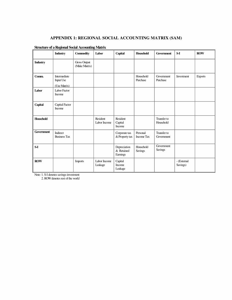
APPENDIX 1: REGIONAL SOCIAL ACCOUNTING MATRIX (SAM)

Structure of a Regional Social Accounting MatrixIndustry Commodity Labor Capital Household Government S-I ROW

Industry Gross Output(Make Matrix)

Comm. IntermediateInput Use

(Use Matrix)

HouseholdPurchase

GovernmentPurchase

Investment Exports

Labor Labor FactorIncome

Capital Capital FactorIncome

Household ResidentLabor Income

ResidentCapitalIncome

Transfer toHousehold

Government IndirectBusiness Tax

Corporate tax& Property tax

PersonalIncome Tax

Transfer toGovernment

S-I Depreciation& RetainedEarnings

HouseholdSavings

GovernmentSavings

ROW Imports Labor IncomeLeakage

CapitalIncomeLeakage

- (ExternalSavings)

Note: 1. S-I denotes savings-investment 2. ROW denotes rest of the world

APPENDIX 2: SOCIAL ACCOUNTING MATRIX (SAM) FOR FISHERIES (Houshak et al., 1997)

Social Accounting Matrix with Disaggregated Fishery SectorsHARVESTINGSECTORS

PROCESSINGSECTORS

NONFISHERYSECTORS

HARVESTINGCOMMOD

PROCESSINGCOMMOD

NONFISHERYCOMMOD

LABOR CAPITAL HOUSEHOLD

GOV’T SAVINGS-INVESTMENT

REST OFWORLD

Harvestingsectors

MakematrixM1

MakematrixM2

MakematrixM3

Processingsectors

MakematrixM4

MakeMatrixM5

MakematrixM6

Nonfisherysectors

MakematrixM7

MakematrixM8

MakeMatrixM9

Harvestingcommodities

Use matrixU1

Use matrixU2

Use matrixU3

HouseholdPurchaseH1

Gov’tPurchaseG1

InvestmentIN1

ExportsE1

Processingcommodities

Use matrixU4

Use matrixU5

Use matrixU6

HouseholdPurchaseH2

Gov’tPurchaseG2

InvestmentIN2

ExportsE2

Nonfisherycommodities

Use matrixU7

Use matrixU8

Use matrixU9

HouseholdPurchaseH3

Gov’tPurchaseG3

InvestmentIN3

ExportsE3

Labor LaborincomeL1

LaborincomeL2

LaborincomeL3

Capital CapitalincomeK1

CapitalincomeK2

CapitalincomeK3

Household ResidentLaborIncome

ResidentCapitalIncome

Transfer toHousehold

Gov’t Indirectbusiness taxT1

Indirectbusiness taxT2

Indirectbusiness taxT3

Corporatetax &Property tax

PersonalIncome Tax

Transfer toGov’t

Savings-investment

Depreciation &RetainedEarnings

HouseholdSavings

Gov’tSavings

Rest ofworld

ImportsIM1

ImportsIM2

ImportsIM3

LaborIncomeLeakage

CapitalIncomeLeakage

- (ExternalSavings)

APPENDIX 3: CGE MODELLING IN PRACTICE

Baseline Simulation BaselinePolicies

Calibration toequilibrium

EconometricAnalysis ofBehaviouralparameters

SAM database

Policy Experiments CounterfactualSimulation

Analysis ofComparativePerformance

Model Design

New Data / New issuesNew structures

New BehaviouralAssumptions

APPENDIX 4: SETS, PARAMETERS and VARIABLES (Salerno-CGE Model) SETS a ∈ A activities c ∈ C commodities c ∈ CM ( C) imported commodities c ∈ CNM ( C) nonimported commodities c ∈ CE ( C) exported commodities c ∈ CNE ( C) nonexported commodities f ∈ F factors h ∈ H ( I) households i ∈ I institutions (households, government, and rest of world) PARAMETERS ada production function efficiency parameter aqc shift parameter for composite supply (Armington) function atc shift parameter for output transformation (CET) function icaca quantity of c as intermediate input per unit of activity a mpsh share of disposable household income to savings pwec export price (foreign currency) pwmc import price (foreign currency) qgc government commodity demand qinvc base-year investment demand shryhf share of the income from factor f in household h tec export tax rate tmc import tariff rate tqc sales tax rate trii' transfer from institution i' to institution i tyh rate of household income tax αfa value-added share for factor f in activity a βch share of commodity c in the consumption of household h δcq share parameter for composite supply (Armington) function δct share parameter for output transformation (CET) function θac yield of commodity c per unit of activity a ρcq exponent (−1 < ρcq < ∞) for composite supply (Armington) function ρct exponent (1 < ρct < ∞) for output transformation (CET) function σcq elasticity of substitution for composite supply (Armington) function σct elasticity of transformation for output transformation (CET) function VARIABLES EG government expenditure EXR foreign exchange rate (domestic currency per unit of foreign currency) FSAV foreign savings IADJ investment adjustment factor PAa activity price PDc domestic price of domestic output PEc export price (domestic currency)

PM import price (domestic currency) PQc composite commodity price PVAc value-added price PXc producer price QAa activity level QDc quantity of domestic output sold domestically QEc quantity of exports QFfa quantity demanded of factor f by activity a QFSf supply of factor f QHch quantity of consumption of commodity c by household h QINTc quantity of intermediate use of commodity c by activity a QINVc quantity of investment demand QMc quantity of imports QQc quantity supplied to domestic commodity demanders (composite supply) QXc quantity of domestic output WALRAS dummy variable (zero at equilibrium) WFf average wage (rental rate) of factor f WFDISTfa wage distortion factor for factor f in activity a YFhf transfer of income to household h from factor f YG government revenue YHh household income EQUATIONS Import Price PMc = (1 + tmc ) ⋅EXR⋅pwmc c ∈CM Export Price PEc = (1 − tec ) ⋅EXR⋅pwec c ∈CE Absorption PQc ⋅QQc = [PDc∈QDc + (PMc ⋅QMc )| c∈CM](1 + tqc ) c ∈C Domestic Output Value PXc ⋅QXc = PDc ⋅QDc + (PEc ⋅QEc )| c∈CE c ∈C Activity Price PAa = Σ PXc ⋅ θac a ∈ A Value-added Price PVAa = PAa − Σ PQc ⋅ icaca a ∈ A Production and Commodity Block Activity Production Function QAa = ada⋅∏f∈F Qffa αfa a ∈ A Factor Demand WFf ⋅WFDISTfa = (afa⋅PAa⋅QAa)/QFfa

Intermediate demand QINTca = icaca ⋅QAa c ∈C, a ∈A Output Function QXc = Σ θac ⋅ QAa c ∈ C Composite Supply (Armington) Function

QQc = aqc ⋅ (δcq ⋅QMcqcρ−

+ (1 − δcq) ⋅QDcqcρ−

)qcρ

1−

c ∈CM Import-Domestic Demand Ratio

qc

PMPD

QDQM

qc

qc

c

c

c

cρ

δδ +

−=

1

1

)1

.(

Composite Supply for Nonimported Commodities QQc = QDc c ∈ CNM Output Transformation (CET) Function

tc

tc

tc

ctcc

tccc QDQEatQX ρρρ δδ

1

)*)1(1( −++= c ∈CE Export-Domestic Supply Ratio

1

1

)1

*( −−=

tc

tc

tc

c

c

c

c

PDPE

QDQE ρ

δδ

c ∈CEQDc PDc δct

Output Transformation for Nonexported Commodities QXc = QDc c ∈ CNE Institution Block Factor Income YFhf = shryhf ⋅Σ WFf ⋅WFDISTfa ⋅QFfa h ∈ H, f ∈ F Household Income YHh = Σ YFhf + trh,gov + EXR⋅ trh,row h ∈ H Household Consumption Demand

c

hhhchch PQ

YHtympsQH

)1)(1( −−=

β

Investment Demand QINVc = qinvc ⋅IADJ c ∈ C

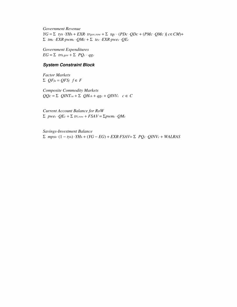
Government Revenue YG = Σ tyh ⋅YHh + EXR⋅ trgov,row + Σ tqc ⋅ (PDc ⋅QDc + (PMc ⋅QMc )| c∈CM)+ Σ tmc ⋅EXR⋅pwmc ⋅QMc + Σ tec ⋅EXR⋅pwec ⋅QEc Government Expenditures EG = Σ trh,gov + Σ PQc ⋅ qgc System Constraint Block Factor Markets Σ QFfa = QFSf f ∈ F Composite Commodity Markets QQc = Σ QINTca + Σ QHch + qgc + QINVc c ∈ C Current Account Balance for RoW Σ pwec ⋅QEc + Σ tri,row + FSAV = Σpwmc ⋅QMc Savings-Investment Balance Σ mpsh⋅ (1 − tyh) ⋅YHh + (YG − EG) + EXR⋅FSAV= Σ PQc ⋅QINVc + WALRAS

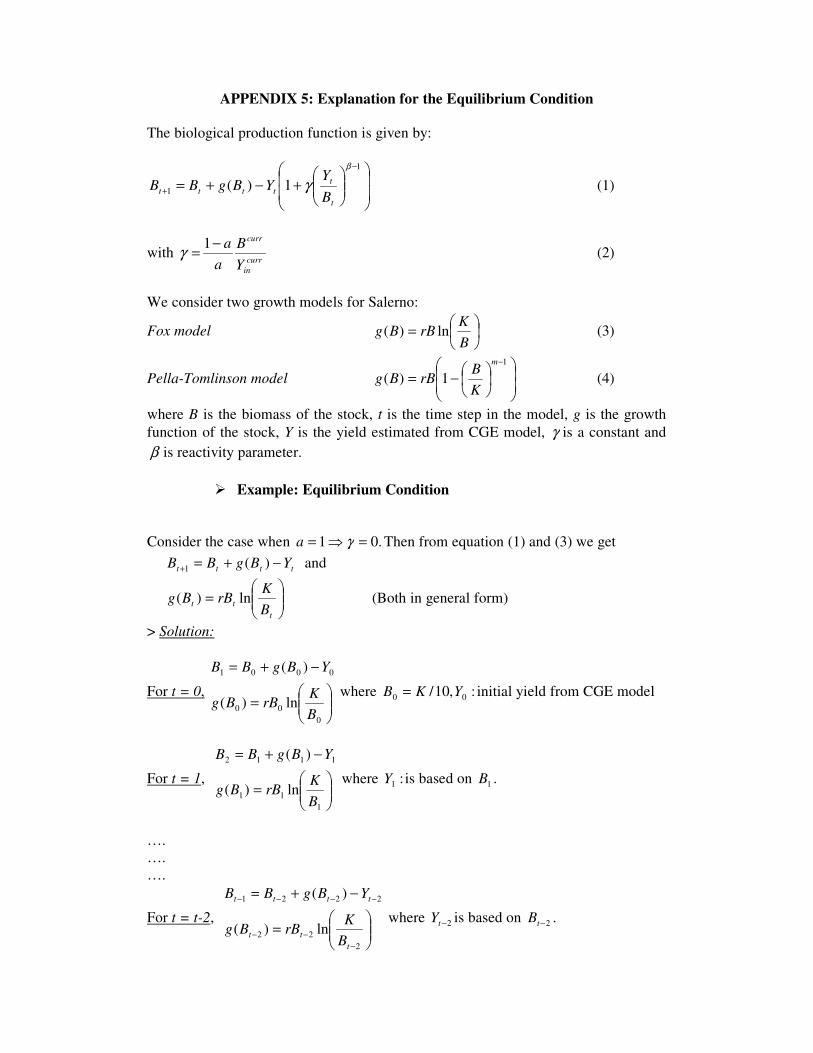
APPENDIX 5: Explanation for the Equilibrium Condition The biological production function is given by:

��

�

�

��

�

�

���

����

�+−+=

−

+

1

1 1)(β

γt

ttttt B

YYBgBB (1)

with curr

in

curr

YB

aa−= 1γ (2)

We consider two growth models for Salerno:

Fox model ��

���

�=BK

rBBg ln)( (3)

Pella-Tomlinson model ��

�

�

��

�

���

���

�−=−1

1)(m

KB

rBBg (4)

where B is the biomass of the stock, t is the time step in the model, g is the growth function of the stock, Y is the yield estimated from CGE model, γ is a constant and β is reactivity parameter.

��Example: Equilibrium Condition Consider the case when .01 =�= γa Then from equation (1) and (3) we get tttt YBgBB −+=+ )(1 and

���

����

�=

ttt B

KrBBg ln)( (Both in general form)

> Solution:

For t = 0, ���

����

�=

−+=

000

0001

ln)(

)(

BK

rBBg

YBgBB

where :,10/ 00 YKB = initial yield from CGE model

For t = 1, ���

����

�=

−+=

111

1112

ln)(

)(

BK

rBBg

YBgBB

where :1Y is based on 1B .

…. …. ….

For t = t-2, ���

����

�=

−+=

−−−

−−−−

222

2221

ln)(

)(

ttt

tttt

BK

rBBg

YBgBB

where 2−tY is based on 2−tB .

For t = t-1, ���

����

�=

−+=

−−−

−−−

111

111

ln)(

)(

ttt

tttt

BK

rBBg

YBgBB

where 1−tY is based on 1−tB .

Final step, ���

����

�=

−+=+

ttt

tttt

BK

rBBg

YBgBB

ln)(

)(1

where tY is based on tB .

��Equilibrium condition: ( )tttt YBgBB =�= + )(,1

tttttt

tttttttttttt

YBgBYBgB

YYBgBgBBYBgBYBgB

−=−−+�

�−−−=−�−+=−+�

−−−

−−−−−−

)()(

)()()()()(

111

111111

Then, the equilibrium condition (state) holds when:

.0)()( 111 =−+− −−− tttt YBgBB Or

111 )( −−− −+= tttt YBgBB (That is true, when t = t-1)

Notes:

1. We start with an initial value for biomass Bo (=K/10). At each iteration t+1,

1+tB is estimated from Bt, g(Bt) and Yt. Each time Bt is given by previous iteration, g(Bt) by biological function and Yt by economic model.

2. Each time, biomass B is a new value, which then gives a new g(B) and Y. So,

at each step i, Yi is based on Bi and used to estimate Bi+1 (i.e. the equilibrium biomass corresponding to Yi).

3. Finally, the model should be converged, and equilibrium condition holds

under g(Bt)=Yt, where B and Y are in steady state.