Developing Climate Change Impacts and Adaptation Metrics for Agriculture Cynthia Rosenzweig and Francesco N. Tubiello Climate Impacts Group NASAGISS and Columbia University

23 June 2006

Produced for the Global Forum on Sustainable Development on the

Economic Benefits of Climate Change Policies

6-7 July 2006, Paris, France

Session 2: Metrics

2

Executive Summary pg. 3

1.0 Introduction pg. 6

2.0 Climate Change and Agriculture pg. 8

2.1 Scenarios for Agricultural Impacts, 1990-2100 pg. 11

3.0 Climate Change and Agriculture Metrics pg. 15

3.1 Key Concepts pg. 15

4.0 Methodologies pg. 18

4.1 Economic Tools pg. 19

4.2 Benchmarks pg. 21

4.3 Current State pg. 22

4.4 Recent Trends pg. 23

4.5 Socio-Economic Development Pathways pg. 24

4.6 Future Climate Change Impacts pg. 24

5.0 Metrics Estimation pg. 25

5.1 Climate Indexes for Regional Impacts pg. 26

5.2 Draft Metrics pg. 27

6.0 Impacts and Economic Valuation Models pg. 30

7.0 Conclusions pg. 33

8.0 References pg. 34

Figures pg. 37

Appendix A. Workshop Report and Case Study Summary pg. 41

Appendix B. Draft CCIAM Metrics Survey pg. 54

3

EXECUTIVE SUMMARY

Development of Metrics for Climate Change and Agriculture

The purpose of this report is to explore useful metrics needed for estimating the short-

term (20-30 years) and long-term (80-100 years) impacts of climate change on

agriculture, both in monetary and non-monetary terms, helping decision–makers

evaluate, at regional to national levels, which adaptation strategies and policy options

potentially minimize risk and maximize benefits under changed climate regimes.

Metrics can help stakeholders and policy-makers assess levels of risk and

vulnerability of agricultural systems, by helping to quantify thresholds beyond which

substantial changes in management practices and concerted action for planned

adaptation strategies is necessary. The Third Assessment Report of the

Intergovernmental Panel on Climate Change (IPCC) Working Group II states that

climate change impacts on agriculture will have local, regional, and global dimensions

(IPCC, 2001). Responses at all scales will depend on the capacity of agricultural

systems to adapt to changed conditions as a function not only of climate, but also of

socio-economic conditions, technological progress and agricultural markets. It is

therefore helpful to develop, together with agricultural stakeholders and decision-

makers, a set of metrics for use in the analysis of the timing and magnitude of such

impacts, and in the evaluation of adaptation actions. A cohesive set of metrics for

climate change and agriculture would facilitate effective planning and implementation

of response strategies at relevant scales and elucidate connections among biophysical

and socio-economic systems. Such an effort contributes to the more robust estimation

of the benefits of climate change policies relating to agriculture.

Climate Change and Agriculture Metrics

A set of “metrics,” or indexes, can be defined as a system of measurement that

includes the item being measured, the unit of measurement, and the value of the unit.

Metrics may provide a tool for developing and implementing response strategies,

measuring progress, and improving performance. Three main principles underlie

development and choice of metrics:

(1) Criteria for selection;

(2) Action plan for metric creation; and

(3) Strategies for use as tools to drive system progress.

4

Following these principles, we provide herein some proposed guidelines on how to

identify and develop a set of Climate Change and Agriculture Metrics, in order to

associate the magnitude and timing of climate change—temperature and precipitation

regimes, necessary to project agricultural risks—with measures of impacts on

agriculture, at regional to national scales, with the aim of helping decision-makers to

devise adaptation strategies. Specifically, metrics should highlight potential physical,

agro-ecological and socio-economic risks, taking into consideration adaptation within

national and sub-national geopolitical units (e.g., states, provinces, regions) and in a

variety of countries. They should provide policy-makers and managers with a tool to

analyze a range of available adaptation options in terms of timing and cost, given a

range of expected outcomes in the face of climate change impacts.

We identify three steps for developing effective metrics:

First, metrics for climate risk in the agricultural sector need to be defined at

various scales, up to national level. These metrics include potential biophysical risks

in the sector (e.g., potential impacts on production and crop yields), socio-economic

indicators (e.g., GDP(A)/capita, commodity prices, food security), and bioclimatic

indices (e.g., temperature, precipitation, and other variables such as droughts and

floods).

Second, metrics that map adaptation options—both autonomous and

planned— against their effectiveness, need to be included. Examples are farm-level

management strategies, regional-level market and policy adjustments that have the

ability to diminish or counterbalance climate impacts, once given threshold levels for

risk are exceeded. Measures of adaptation options should likewise include an

indication of synergy with mitigation strategies, i.e., favouring solutions that also

facilitate reduction of greenhouse gas concentrations in the atmosphere.

Third, preliminary sets of metrics need to be tested for their efficacy as tools

for easily-communicated and relevant information for stakeholders and policy-

makers. To gather feedback on this aspect, we invited a group of international

stakeholders to help us identify and select, through a workshop process, useful sets of

agricultural impact and response metrics.

5

An initial set of metrics was chosen based on a literature review (based on the

IPCC, United Nations Framework Convention on Climate Change (UNFCCC), U.S.

and UN Development Programme (UNDP) Country Studies, and other national

reports), previous climate change and agriculture impact studies, and expert

consultation with agronomists, climate impacts specialists, resource economists, and

risk and adaptation specialists. Measures of uncertainties were also included.

Four case studies were used to provide testing of various metrics against

different levels of government and agricultural systems, in developed, developing and

transition countries:

(1) Developed Country: U.S. Production;

(2) Developing Country Semi-Arid Tropical Agriculture: South-East South

America;

(3) Economy in Transition High-Latitude Agriculture: Slovakia and Ukraine; and

(4) Mediterranean Semi-arid Environments.

Aknowledgements

We gratefully acknowledge funding by OECD that made this project possible. The

ideas and tools proposed in this paper were the result of fruitful and engaging

interactions with many individuals having backgrounds spanning a wide spectrum of

expertise, from agronomists and crop modelers to economists and social scientists,

and including contributions from government experts. We would like to thank in

particular those who helped us test our initial ideas against specific case studies: Livia

Bizik (Slovakia and Ukraine); Bill Easterling (U.S. and IPCC); Walter Baethgen

(Uruguay and Latin America); Francesco Zecca, Marcello Donatelli, and Donatella

Spano (Italy and Mediterranean Environments).

6

1. Introduction

The Third Assessment Report of the Intergovernmental Panel on Climate Change

Working Group II states that climate change impacts on agriculture will have local,

regional, and global dimensions (IPCC, 2001b). Responses at all scales will depend

on the capacity of agricultural systems to adapt to changed conditions as a function,

not only of climate, but also of socio-economic conditions, technological progress and

agricultural markets. It is therefore useful to develop, together with agricultural

stakeholders and decision-makers, a set of metrics for analysis of the timing and

magnitude of such impacts, quantification of potential damages and benefits, and thus

in the evaluation of adaptation strategies that help minimize risk and maximize

benefits under future climates. A cohesive set of metrics for climate change and

agriculture will facilitate effective planning and implementation of response strategies

at the various scales and elucidate connections among biophysical and socio-

economic systems. Such an effort contributes to the more robust estimation of the

benefits of climate change policies relating to agriculture, including practical,

operational definitions of risk and vulnerability thresholds for agricultural systems.

As a matter of definition, agricultural production systems considered herein

can be defined as ‘groups of enterprises that integrate agronomic elements (e.g.,

climate, soils, crops and livestock) with economic elements (e.g., material, labor, and

energy inputs; food and services outputs).’ These are affected by socio-economic and

cultural processes at local, regional, national, and international scales, including

markets and trade, policies, trends in rural/urban population, and technological

development. Each agricultural production system thus possesses specific

characteristics related to these differing scales. For the purpose of this work, we focus

on regional and national scales, as these seem to be appropriate for development of

metrics related to climate change and agriculture, and their use in implementation of

adaptation and mitigation strategies. When appropriate, global perspectives are

explicitly described by the climate, socio-economic and policy trends underlying the

analysis.

This study considered criteria for developing metrics to assess risks to the

agricultural sector arising from potential changes in mean and distribution of

7

temperature and precipitation over the next 100 years, useful to identifying strategies

and methods related to adaptation. The paper is organized in three parts:

(1) Overview of climate change impacts on the agricultural sector over the 21st

century (Section 2).

(2) Policy-relevant metrics for assessing agricultural risks and for adaptation

planning. The set of metrics discussed associate the magnitude and timing of

climate change with impacts on production, rural welfare and agricultural

economies. This includes a focus on both short-term (20-30 years) and long-

term (80-100 years) risks. Criteria for the relevance of metrics to decision-

makers at different levels of government, and their utility for widespread

communication are discussed. This aspect was informed by the workshop of

relevant stakeholders to review the utility of the selected metrics, and to

refine, add, and discuss issues of importance to different constituents and

regions (Section 3).

(3) Methodology, frameworks for metric estimation, and an analysis of the utility

of current dynamic crop decision tools and economic valuation models.

Methods for impact assessments with adaptation were considered in four

case studies, spanning both developing and developed country agricultural

systems in the U.S., Slovakia and Ukraine, Italy and southern Mediterranean,

and Uruguay and Latin America. Relevant information is also included on

datasets and selected assessment models and methodologies for quantifying

risk to agricultural production and economic value (Sections 4 and 5).

The following sections discuss each of these components. Additional

background material, such as the climate scenarios and the workshop report, are

provided in the Appendixes.

8

2.0 Climate Change and Agriculture

There is concern about the impacts of climate change and variability on agricultural

production worldwide. At the global scale, food security is situated prominently on

the list of human activities and ecosystem services under threat of dangerous

anthropogenic interference on earth’s climate (Millennium Ecosystem Assessment

2005; IPCC 2001a; Watson et al. 2000; article II, UNFCCC). Individual countries

may be concerned with potential damages and benefits that may arise over the coming

decades from climate change impacts on their territories as well as globally, since

these are likely to affect domestic and international policies, trading patterns, resource

use, regional planning, and the welfare of their citizens.

Current research confirms that, while crops would respond positively to

elevated CO2 in the absence of climate change (e.g., Ainsworth and Long 2005;

Kimball et al. 2002; Jablonski et al. 2002), the associated impacts of high

temperatures, altered patterns of precipitation, and possibly increased frequency of

extreme events such as droughts and floods will likely combine to depress yields and

increase production risks in many regions over time (e.g., IPCC 2001b; Tab. 1).

Table 1. Some possible climate change agro-ecosystem impacts and management

responses

Agro-Ecosystem Impact Possible Adaptation Response Biomass increase under elevated CO2 Cultivar selection to maximize yield Acceleration of maturity due to higher T Cultivar selection with slower maturing

types/crop shifts Heat stress during flowering and reproduction

Early planting of spring crops

Crop losses due to increased variability; Drought/flooding

Crop mixtures/rotation change; change in soil and water management; early warning systems

Increased competition/pests Land and input management

A consensus has emerged that developing countries are more vulnerable to

climate change than developed countries, because of the predominance of agriculture

in their economies, the scarcity of capital for adaptation measures, their warmer

baseline climates, and their heightened exposure to extreme events (Parry et al. 2001;

IPCC, 2001). Thus climate change may have particularly serious consequences in the

9

developing world, where about 800 million people are currently undernourished (e.g.,

UN Millennium Project , 2005).

Many interactive processes determine the dynamics of world food demand and

supply: agro-climatic conditions, land resources, and their management are clearly a

key component, but they are critically affected by distinct socio-economic pressures,

including current and projected trends in population growth, as well as availability

and access to technology and development. In the last three decades, for instance,

average daily per capita intake has risen globally from 2,400 to 2,800 calories, spurred

by economic growth, improved production systems, international trade, and

globalization of food markets. Feedbacks of such growth patterns on cultures and

personal taste, lifestyle and demographic changes have in turn led to major dietary

changes – mainly in developing countries, where shares of meat, fat, and sugar to total

food intake have increased significantly (e.g., Fischer et al. 2005).

Several integrated assessment studies have focused on quantifying key impacts

on food production from climate change, as a function of different socio-economic

scenarios, including analyses of likely adaptation strategies such as crop management

changes and economic adjustments (e.g., Fischer et al. 2005; Parry et al. 2004; FAO

2003; Fischer et al., 2002; Rosenzweig and Parry 1994).

Hitz and Smith (2004) summarized potential impacts on the agricultural sector

as a function of global mean temperature change, used as a single metric for the time-

evolution of climate change during this century. In a review of current literature, they

found small overall positive impacts across scenarios and models, up to about 3°C,

and negative impacts above that degree of warming. These results suggest that

agriculture may overall suffer little, or even benefit, from climate impacts in the

coming two-three decades—with positive effects of elevated CO2 on crops overriding

negative temperature signals—but possibly turn negative in the second half of this

century. These results however apply to analyses of changes in mean climate only;

increased frequencies of extreme events may tip the balance towards negative impacts

earlier in this century.

10

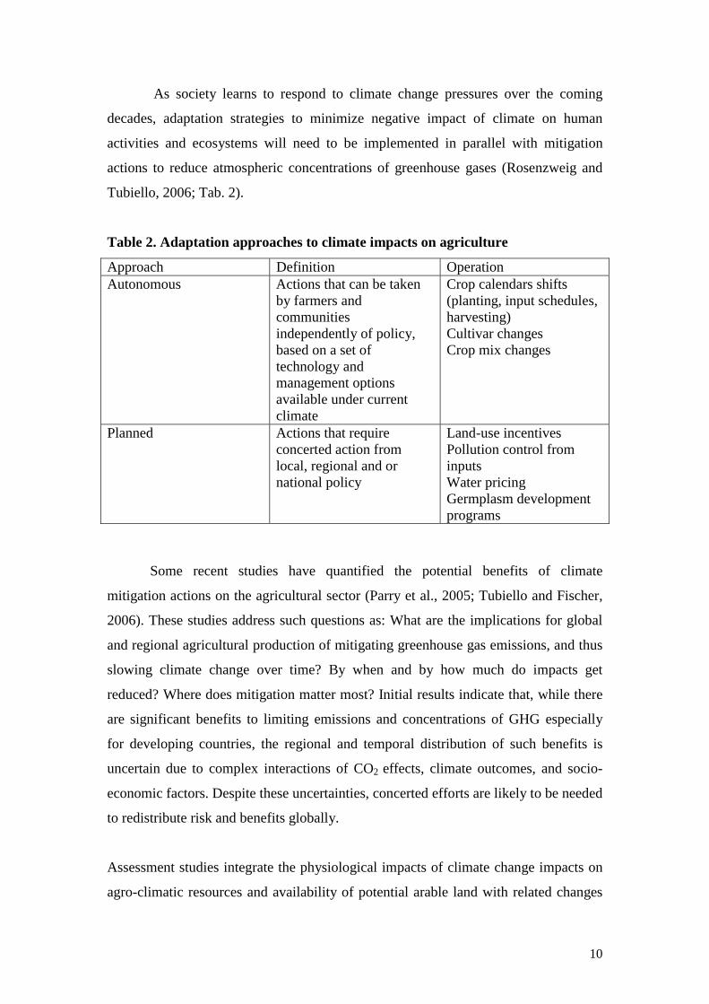
As society learns to respond to climate change pressures over the coming

decades, adaptation strategies to minimize negative impact of climate on human

activities and ecosystems will need to be implemented in parallel with mitigation

actions to reduce atmospheric concentrations of greenhouse gases (Rosenzweig and

Tubiello, 2006; Tab. 2).

Table 2. Adaptation approaches to climate impacts on agriculture

Approach Definition Operation Autonomous Actions that can be taken

by farmers and communities independently of policy, based on a set of technology and management options available under current climate

Crop calendars shifts (planting, input schedules, harvesting) Cultivar changes Crop mix changes

Planned Actions that require concerted action from local, regional and or national policy

Land-use incentives Pollution control from inputs Water pricing Germplasm development programs

Some recent studies have quantified the potential benefits of climate

mitigation actions on the agricultural sector (Parry et al., 2005; Tubiello and Fischer,

2006). These studies address such questions as: What are the implications for global

and regional agricultural production of mitigating greenhouse gas emissions, and thus

slowing climate change over time? By when and by how much do impacts get

reduced? Where does mitigation matter most? Initial results indicate that, while there

are significant benefits to limiting emissions and concentrations of GHG especially

for developing countries, the regional and temporal distribution of such benefits is

uncertain due to complex interactions of CO2 effects, climate outcomes, and socio-

economic factors. Despite these uncertainties, concerted efforts are likely to be needed

to redistribute risk and benefits globally.

Assessment studies integrate the physiological impacts of climate change impacts on

agro-climatic resources and availability of potential arable land with related changes

11

in crop production and economic patterns. These can be used to characterize risks to

the sector over time. Our analyses focus on the decades of this century, up to 2100,

with both a short-term (20-30 years) and a long-term (80-100 years) focus, and with

attention to potential changes in food demand; risks to production, trade and incomes;

and the scale and location of risk of hunger.

2.1 Scenarios for Agricultural Risks, 1990-2100

In order to assess agricultural development over this century, with or without climate

change, it is necessary to first make coherent assumptions about how key socio-

economic drivers of food systems might evolve over the same period, and project

their impact on agriculture—defining a benchmark against which to assess climatic

impacts (see Fig. 1). For this purpose, we considered plausible socio-economic

development paths specified in the IPCC Special Report on Emissions Scenarios

(SRES) (Nakicenovic and Swart, 2000; IPCC, 2001). The four families of SRES

scenarios explore socio-economic development and related pressures on the global

environment in this century, with special reference to emissions of greenhouse gases

into the atmosphere. Within this context, climate change is a consequence of social,

economic, and environmental interactions, possibly modulated by the capacity to

adapt at regional and national levels. Emissions of greenhouse gases connected to

specific SRES scenarios have been translated into projections of climate change by

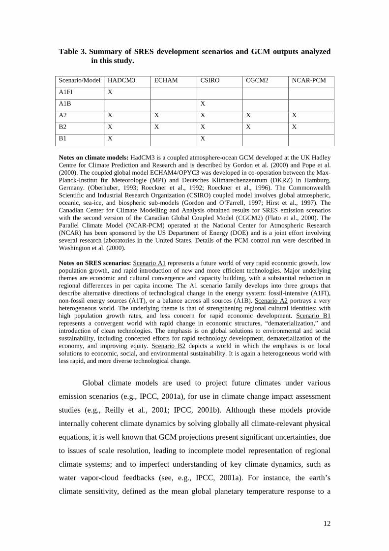
using global climate models (GCMs). We considered climate projections available

from the IPCC Data Distribution Centre and the Climate Research Unit,

corresponding to four families of the SRES emission scenarios: A1, A2, B1, and B2

(see Tab. 3).

12

Table 3. Summary of SRES development scenarios and GCM outputs analyzed in this study.

Scenario/Model HADCM3 ECHAM CSIRO CGCM2 NCAR-PCM

A1FI X

A1B X

A2 X X X X X

B2 X X X X X

B1 X X

Notes on climate models: HadCM3 is a coupled atmosphere-ocean GCM developed at the UK Hadley Centre for Climate Prediction and Research and is described by Gordon et al. (2000) and Pope et al. (2000). The coupled global model ECHAM4/OPYC3 was developed in co-operation between the Max-Planck-Institut für Meteorologie (MPI) and Deutsches Klimarechenzentrum (DKRZ) in Hamburg, Germany. (Oberhuber, 1993; Roeckner et al., 1992; Roeckner et al., 1996). The Commonwealth Scientific and Industrial Research Organization (CSIRO) coupled model involves global atmospheric, oceanic, sea-ice, and biospheric sub-models (Gordon and O’Farrell, 1997; Hirst et al., 1997). The Canadian Center for Climate Modelling and Analysis obtained results for SRES emission scenarios with the second version of the Canadian Global Coupled Model (CGCM2) (Flato et al., 2000). The Parallel Climate Model (NCAR-PCM) operated at the National Center for Atmospheric Research (NCAR) has been sponsored by the US Department of Energy (DOE) and is a joint effort involving several research laboratories in the United States. Details of the PCM control run were described in Washington et al. (2000). Notes on SRES scenarios: Scenario A1 represents a future world of very rapid economic growth, low population growth, and rapid introduction of new and more efficient technologies. Major underlying themes are economic and cultural convergence and capacity building, with a substantial reduction in regional differences in per capita income. The A1 scenario family develops into three groups that describe alternative directions of technological change in the energy system: fossil-intensive (A1FI), non-fossil energy sources (A1T), or a balance across all sources (A1B). Scenario A2 portrays a very heterogeneous world. The underlying theme is that of strengthening regional cultural identities; with high population growth rates, and less concern for rapid economic development. Scenario B1 represents a convergent world with rapid change in economic structures, “dematerialization,” and introduction of clean technologies. The emphasis is on global solutions to environmental and social sustainability, including concerted efforts for rapid technology development, dematerialization of the economy, and improving equity. Scenario B2 depicts a world in which the emphasis is on local solutions to economic, social, and environmental sustainability. It is again a heterogeneous world with less rapid, and more diverse technological change.

Global climate models are used to project future climates under various

emission scenarios (e.g., IPCC, 2001a), for use in climate change impact assessment

studies (e.g., Reilly et al., 2001; IPCC, 2001b). Although these models provide

internally coherent climate dynamics by solving globally all climate-relevant physical

equations, it is well known that GCM projections present significant uncertainties, due

to issues of scale resolution, leading to incomplete model representation of regional

climate systems; and to imperfect understanding of key climate dynamics, such as

water vapor-cloud feedbacks (see, e.g., IPCC, 2001a). For instance, the earth’s

climate sensitivity, defined as the mean global planetary temperature response to a

13

doubling of CO2 levels (~560 ppm) in the atmosphere, is thought to be in the 1.5-

4.5°C range (IPCC, 2001a). Even among GCMs with similar climate sensitivities and

thus temperature change simulations, predictions of regional precipitation responses

may vary significantly, due in part to the intrinsic chaotic nature of climate, and in

part to differences in model approaches to resolving local-to-regional atmospheric

dynamics.

We considered climate change scenarios based on five GCMs: HadCM3,

ECHAM4, CSIRO, CGCM2, and NCAR, in order to summarize the current range of

potential changes in mean temperature and precipitation. Climate sensitivities of the

first four models lie in the upper portion of the IPCC range, while the NCAR model

has a lower climate sensitivity. This is shown by pooling mean annual temperature

projections of all models against CO2 concentrations (a proxy for time, as CO2 may

increase at a rate of 0.5-1% per annum over this century) (Fig. 2). There is some

correlation between climate projections of mean annual temperature and precipitation

over land at mid-to-high latitudes (Fig. 2a), where most developed countries are

located, but none at tropical latitudes (Fig. 2b), where most developing countries are

located.

Recent results from an agro-ecological zone model coupled with an economic

trade model, AEZ-BLS, used in conjunction with such scenarios (Fischer et al., 2005),

exemplify typical response curves for agricultural production, highlighting critical

differences between developed and developing countries (Fig. 3). Such modeling

approaches often follow a two-step simulation strategy, analyzing impacts with and

without climate change, in order to separate the impacts of climate change on

agriculture, in particular higher temperature, modified rainfall patterns and elevated

CO2 concentrations, from the effects of concomitant socio-economic trajectories.

Simulation models provide a valid, and often the only available, tool used in

investigations of complex interactions and feedbacks of many variables. Several limits

and uncertainties are linked to such exercises. Firstly, GCMs results represent

physically plausible future climates, rather than exact predictions. As a consequence,

assessment studies of climate impacts on agriculture—especially given the prominent

role played by rainfed production worldwide—should not depend on one GCM alone,

14

but use several climate predictions (Tubiello and Ewert, 2002). Particularly in

agriculture, the direction of predicted precipitation can largely shape regional results.

At the same time, most assessment studies have not yet included the potential for

changes in the frequency of extreme events. As shown in Rosenzweig et al. (2002),

projected agricultural outcomes tend to become more negative under scenarios that

consider increased variability in hydrological regimes (i.e., more droughts and floods)

as projected in GCMs.

Secondly, simulation results depend strongly on crop and economic model

dynamics. Although most models have been validated for past periods and many sites,

various additional and uncertain assumptions are needed to project food-system

dynamics at large regional scales and through time (e.g., scaling issues from site to

region; technical progress in crop yields; regional irrigation development; changes in

food preferences; etc.). In addition, simulated crop response to elevated CO2—derived

from experimental data—may be larger than actually possible at farm levels. Finally,

the SRES scenarios have recently been criticized for their some of their regional

economic growth patterns, regarded as too strong when compared to historical data

(e.g., see Navicekovic et al., 2003).

3.0 Climate Change Impacts and Adaptation Metrics

The proposed Climate Change Impacts and Adaptation Metrics (CCIAM) are

designed to be useful with regard to monitoring and responding to climate change.

This includes the ability to classify severity of impacts; a system’s capacity to respond

to climate change; and rate adaptation options to take advantage of beneficial changes

or minimize damage. Importantly, such metrics can help decision-makers to assess the

risks to and vulnerability of a system to increasing degrees of climate change,

identifying thresholds beyond which current coping capacity and autonomous

adaptation responses may need to be complemented by planned adaptation responses

at local to regional levels, involving significant changes in management practices

(Jones, 2003; 2001). Thus, CCIAM includes biophysical and agro-climatic

dimensions, as well as critical socio-economic, cultural, institutional and political

aspects. They should also consider trade protectionism, hunger, and environmental

pressures and/or pollution, in order to be meaningful to policy-makers. Ultimately,

15

metrics should communicate in a simple and concise manner a sense of how important

the risks of climate change to agriculture are; to what extent adaptation can be

effective; and ultimately the extent to which decision-makers should take action.

Criteria for selection of the CCIAM Metrics are identified as:

(1) Relevancy to monitoring and responding to climate change;

(2) Appropriateness for regional and/or national level agriculture planning; and

(3) Availability of observed or model-generated data.

An important caveat to any metric is that there may be important differences both

within and across regions. A given farming region might be doing well overall even

though some single producers within it may be failing while others prosper; another

region might thrive at the expense of others due to effective regional policies or

markets. The workshop participant helped us to evaluate criteria as well as a candidate

set of metrics.

3.1 Key Concepts

A set of metrics can be defined as a system of measurement, one that can be used in

an objective, transparent, and reproducible manner to describe the characteristics and

transformations of observable systems. Metrics carry with them – implicitly or

explicitly – a definition of the system being measured, as well as the set of

measurement units to be used. Within the context of this work, criteria for developing

agricultural metrics were investigated, in order to define and characterize the status of

given agricultural production systems against the changing climate of the coming

decades, with a focus on both short-term (20-30 years) and long-term (80-100 years)

horizons. The underlying idea in this exercise is that a set of such metrics can be used

by decision-makers to provide an easy-to-understand “health report,” or a snapshot of

an agricultural system, with regard to the likely risks of climate change impacts in

coming decades. This implies that efforts to this end should be focused on developing

a ‘minimum set’ of metrics to enhance their utility to plan in a timely manner

adaptation strategies aimed at minimizing risk and maximizing benefits potentially

arising from changed sets of climatic parameters.

16

In addition to defining the system to be measured and a minimum set of

metrics, it is necessary to define a framework and a set of classification schemes, or

benchmark values, against which to interpret the metrics. For instance, assessing the

impacts of, and adaptation responses to, future changes in mean and variability

distributions of temperature and precipitation over coming decades should include the

socio-economic evolution of that system in coming decades, compared to today, so

that the additional changes due to climate change can be clearly estimated. Finally and

importantly, the choice of metrics may depend on the scale of interest, from local to

regional, from national to global. The focus of this work is to provide criteria for

developing metrics that can be used at national scales.

Adaptive capacity of a system, in the context of climate change, can be

defined as the full set of system skills, i.e., technical solutions available to farmers in

order to respond to climate change stress, as determined by the socio-economic and

cultural backgrounds, plus institutional and policy contexts, prevalent in the region of

interest.

Adaptation to climate change can be defined as the full set of actions actually

taken in response to changes in local and regional climatic conditions (Smit et al.,

2000). In addition, system response to socio-economic, institutional, political or

cultural pressures may outweigh response to climate change alone in driving the

evolution of agricultural systems (de Loe et al., 2000).

While adaptive capacity could in principle be defined a priory, given a

theoretical framework stating the relative importance of its various component factors,

adaptation is by definition an a-posteriori concept. In particular, actual adaptation

may include a subset of the adaptive capacity of a system, but it may also likely

contain a number of solutions outside its adaptive capacity set, due to surprises and

system uncertainties.

Vulnerability of an agricultural system is defined herein—following

discussions in Kates et al. (2000)—as a function of exposure of that system to climate

hazards, its intrinsic sensitivity to that exposure, and its adaptive capacity:

17

Vulnerability = f (Exposure, Sensitivity (Exposure), Adaptive Capacity)

Here adaptive capacity is defined as the full set of system skills (agronomic, socio-

economic, cultural, political/institutional) that allows successful adjustments to

current and future changes in climate variability and means. It follows from the

equation above that vulnerability of given systems could be computed over a range of

potential climatic outcomes, for instance a range of GCM outputs, by keeping

adaptive capacity fixed while varying exposure and sensitivity. Changes through time

in socio-economic backgrounds can additionally be accounted for by varying adaptive

capacity as well.

In practice, in an operational mode within the context of a system of metrics,

vulnerability can be expressed—and any theoretical framework tested against— as the

sum of damage costs experienced over a reference period, and including some

measure of recovery.

Vulnerability thresholds are defined herein in accordance to Jones (2004), as

specific values of the proposed metrics, beyond which the ability of a system to cope

with new climatic ranges is significantly diminished, with increased risk of production

failures. In such cases, significant changes in management practices may be necessary

to restore system productivity at acceptable levels. Although the concept of risk, or

vulnerability thresholds is in part value-laden, in the case of agriculture some

thresholds can be defined objectively. For example, well-defined thresholds may be

based on estimates of national-level interannual yield variability over long-term

means—the coefficients of variation—which provide good indicators of the long-term

viability of production systems; likewise, physiological temperature limits to crop

growth—especially during key phonological events such as flowering—can be used

as thresholds. At the socio-economic level, nutrition indexes, derived from comparing

internal food supply, including trade, with calorie demand, provide important

thresholds that can be set as triggers (e.g., Fischer et al., 2005).

When used to provide a ‘snapshot’ of the current situation, metrics can aid in the

assessment of adaptive capacity and vulnerability of given agricultural systems in the

face of potential warming and increased frequency of extreme events. They can also

18

help to elucidate, as climate change progresses, when interventions become

appropriate and to which systems interventions might be usefully applied. They can

also help to define which adaptation actions are available to minimize risk and/or to

optimize the agricultural system’s state under the changed conditions of future

decades.

4.0 Methodologies

Metrics should enable decision-makers to predict and track system vulnerability (or

robustness) to climate change by estimating degrees of exposure and vulnerability to

that exposure, as well as by characterizing adaptive capacity. As stated above,

vulnerability can be estimated by summing the costs of impacts over a given period of

time, allowing for a measure of system adjustment and related benefits. To this end,

standard economic valuation methods are discussed in the section below.

However, such an estimation of vulnerability has only an a-posteriori value,

since it is designed to operate over a reference period that has already happened. By

contrast, metrics that need to assess vulnerability over a range of potential futures

need to rely on models. After discussing general criteria for assessing metrics against

a framework of temporal evolution of both socio-economic and climate variables

(Section 4), leading to a draft set of proposed climate change and adaptation metrics

(Section 5), we discuss how dynamic crop/decision support models and Ricardian

methods can help compute these metrics over future decades.

4.1 Economic Tools

Three different methods can be used in evaluating impacts and adaptation measures

from an economic perspective: cost benefit analysis, cost effectiveness analysis and

multi criteria analysis. We briefly summarize these tools following WGII of IPCC.

Benefit-cost analysis (BCA): Under benefit cost analysis, the costs of implementing

and maintaining adaptation measures are evaluated against the short and long term

benefits of these measures. BCA entails: a) identification of lifetime benefits and

costs of an adaptation measure; b) conversion of the costs and benefits to a single

19

monetary metric; c) discounting of the future benefits and costs. There are two

components of this type of analysis: calculating net benefit—whether or not the

benefits outweigh the costs; and calculating timing of implementation—at what point

in time the project becomes economically viable. The adaptation measures are ranked

according to the benefit-cost ratio (BCR) or net benefits.

The benefit of early adaptation is expressed as the change in the present value

costs of adaptation now (PVN) and the present value costs of adaptation later (PVL):

(PVN – PVL) = (ACN - ACLδ) + (DCN0 – DCU0) + ∑ (DCNt – DCLt) δt, where

ACN is adaptation costs now; ACL is adaptation costs later; DCN0 is damage costs

now; DCU0 is damage costs at a period later; DCL is subsequent damage costs for

later periods, and δ is the discount rate. The first component of the right hand side of

the equation, (ACN - ACLδ), is the difference in adaptation costs over time. The

second component, (DCN0 – DCU0), calculates the short-term benefits (avoided

costs) of adaptation. The third part, (∑ (DCNt – DCLt) δt) concerns the long-term

benefits of an adaptation measure.

BCA has often been used to evaluate agricultural policies. However,

limitations of the technique include: a) the costs of adaptation are not often clear; b)

the distribution of costs and benefits are not provided; and c) conversion to a single

monetary metric might not account for non-market costs and benefits.

Cost-effectiveness analysis (CEA): CEA calculates the least expensive option to

meet a certain goal. This method is useful in the case when benefits of an adaptation

measure cannot be reliably quantified and there are more than one measure is

available to achieve an adaptation goal. Cost effectiveness can be determined in

terms of cost of measure per unit of incremental benefit. CEA can be conducted using

Adaptation Decision Matrix, which weighs benefits and scores specific adaptation

measures.

Multi-criteria analysis (MCA): MCA takes into account a wide range of criteria,

using multiple evaluation methods. Consideration of costs is one such criterion. The

outcome of an MCA can be expressed with a single index value to reveal the overall

20

merit of specific adaptation measures. MCA techniques can be used to determine

adaptation priorities and to evaluate specific adaptation measures. It involves the

specification of objectives, alternative measures/interventions, evaluation criteria,

scoring of specific measures against the criteria and weights ascribed to the various

criteria. An important aspect of this type of analyses is that it accommodates

stakeholder participation. Mizina et al. (1999) used MCA to examine the adaptation

options for Kazakhstan agriculture under climate change. The downside of using

MCA is that weighing different criteria and measures is subjective and can influence

the final outcome.

4.2 Benchmarks

The setting of benchmarks against which to assess the ‘state’ of a given agricultural

system in relation to climate change is an important challenge to the development of

metrics for agriculture. Benchmarking should address two temporal dimensions

within which to assess system function, climate change impacts and responses. The

first benchmark is the current situation of the agricultural system, including recent

trends, such as regional climate signals and agricultural system responses. The second

benchmark comprises the future of the system, including its reference socio-economic

development without climate change, as well as analyses of potential impacts and

responses to climate change at regional and national level.

1) Present State of the agricultural system at regional and national scales,

comprising:

a) Current State long-term characteristics of production systems;

b) Observed Recent Trends in climate variability, change and responses

2) Future State defined in terms of:

a) Socio-Economic Development Pathway(s) without climate change;

b) Climate Change Impacts Projections related to coping ranges so as to define

risk at several levels of adaptation.

The following sections propose initial sets of metrics for each benchmark and

discuss issues with their related measurements.

4.3 Current State

21

These are metrics that describe current agricultural systems, preferably based on the

long-term sustainability of production. Long-term means (of at least 20 years) and

variability of yield and production, income, and aggregate production values may be

compiled to this end. Regional and national data on income and production, available

from FAO and related studies (e.g., Bruinsma et al. 2003; Fischer et al., 2005, Parry et

al. 2005) may be pooled to describe total and regional GDP, GDP/cap, share of

agricultural GDP (agGDP) and agGDP/cap; total and regional production of cereals

and /or additional crops. Another useful tool is a food sufficiency metric, i.e., an

indicator of the number of people at risk of hunger in a given region, which includes

the effects of trade balances (FAO; Fischer et al., 2005).

Regional agro-climatic statistics include mean and variability of temperature

and precipitation, noting whether the region of interest falls within an important El

Nino-Southern Oscillation (ENSO) pattern; beginning and end of growing season;

mean and variability of temperature and precipitation during the growing season,

mean yield and variability of major crops; mean and variability of area planted, inputs

used (water, N, etc.).

Social and political contexts are also included: presence of specific trading

blocs/protections, major trading partners, and regions that most influence production

choices/dynamics.

These simple tables of metrics—benchmarking the system—are best

organized into classification schemes so that the state and climate vulnerability of

different regions and nations may be highlighted and compared. Table 4 shows one

such classification scheme.

Table 4 Classification of Current State

Classification Region 1 Region 2 Region 3 Development status (Developed, Developing, Economy in transition)

Climate stability (stable, high climate variability (e.g., prone to flooding/droughts)

Limits to current production and yield-gap status (inputs water/N/chemical inputs); identified thresholds

Current adaptation tool-kit Linkages to other regions;

22

Political/institutional context (food self-sufficiency; trade balances; protectionism levels, etc.)

A next step in devising impact and adaptation metrics is to provide evaluation criteria

for the classification matrix above. Additional levels of detail can be added through

contributions by regional stakeholders and experts.

4.4 Recent Trends

Climate metrics for observed recent trends are selected to determine whether the

region of interest has experienced changes in climate means and variability in the last

two decades (see Rosenzweig et al., 2005). A second set of metrics describes impacts

on actual agricultural systems, i.e., changes in management (planting dates, input

management, etc.) and in outputs (production, income). A third set ranks the

adaptations implemented against the tool-kit under the Current State Benchmark. Is

this adaptation being used fully? Are adaptations autonomous, or planned? Are there

‘surprise’ adaptations? Can cost/benefits and/or other economic valuations be

determined? Are thresholds being approached/surpassed? How do these responses fit

into the classification scheme developed for the Current State case?

Including autonomous adaptation as a metric is important in order to

characterize how far from the reference the system is evolving, relative to its baseline

conditions; in addition, it provides for an implicit measure of the multi-dimensional

interactions among climate pressures and all relevant cultural, socio-economic,

political dimensions over and above the agronomic-technological components.

4.5 Socio-Economic Development Pathways

This step in devising metrics requires the development of a number of plausible future

scenarios (i.e., without climate change but as a function of socio-economic

development), alongside those presented earlier in this paper, needed in order to

characterize the time-evolution of the current or reference state. The main

development pathways for the agricultural system include possible trends in rural

population, technological change, and land-use change. These could potentially

23

follow the IPCC SRES scenarios, FAO projections, or other national and international

planning documents.

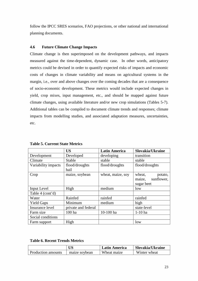
4.6 Future Climate Change Impacts

Climate change is then superimposed on the development pathways, and impacts

measured against the time-dependent, dynamic case. In other words, anticipatory

metrics could be devised in order to quantify expected risks of impacts and economic

costs of changes in climate variability and means on agricultural systems in the

margin, i.e., over and above changes over the coming decades that are a consequence

of socio-economic development. These metrics would include expected changes in

yield, crop mixes, input management, etc., and should be mapped against future

climate changes, using available literature and/or new crop simulations (Tables 5-7).

Additional tables can be compiled to document climate trends and responses; climate

impacts from modelling studies, and associated adaptation measures, uncertainties,

etc.

Table 5. Current State Metrics

US Latin America Slovakia/Ukraine Development Developed developing transition Climate Stable stable stable Variability impacts flood/droughts

hail flood/droughts

flood/droughts

Crop maize, soybean wheat, maize, soy wheat, potato, maize, sunflower, sugar beet

Input Level High medium low Table 4 (cont’d) Water Rainfed rainfed rainfed Yield Gaps Minimum medium high Insurance level private and federal state-level Farm size 100 ha 10-100 ha 1-10 ha Social conditions Farm support High low

Table 6. Recent Trends Metrics

US Latin America Slovakia/Ukraine Production amounts maize soybean Wheat maize Winter wheat

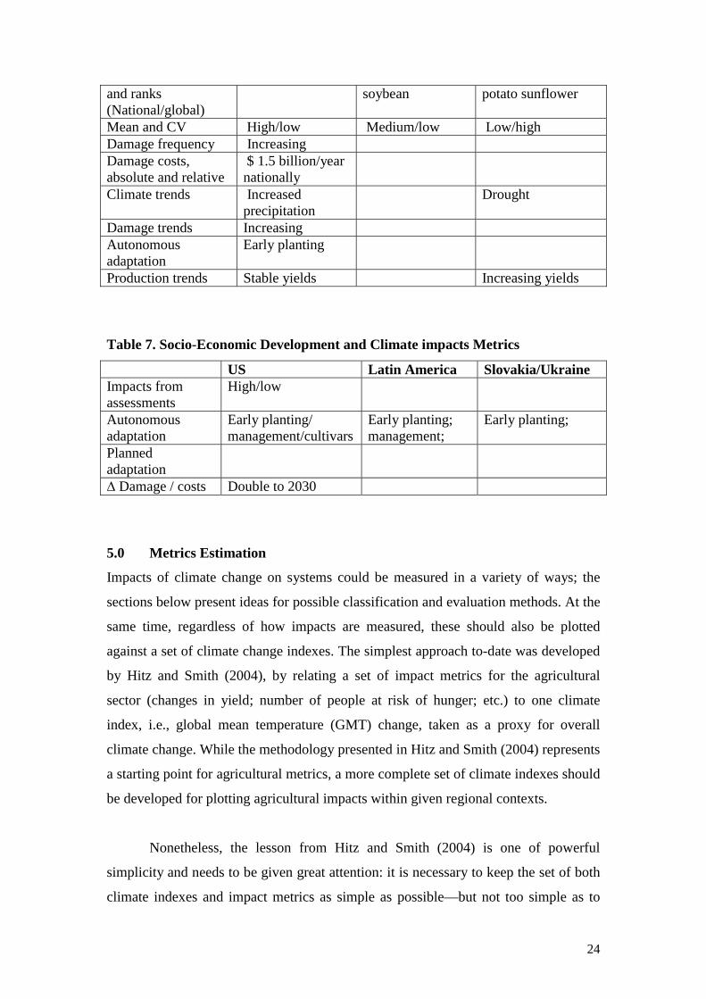
24

and ranks (National/global)

soybean potato sunflower

Mean and CV High/low Medium/low Low/high Damage frequency Increasing Damage costs, absolute and relative

$ 1.5 billion/year nationally

Climate trends Increased precipitation

Drought

Damage trends Increasing Autonomous adaptation

Early planting

Production trends Stable yields Increasing yields

Table 7. Socio-Economic Development and Climate impacts Metrics

US Latin America Slovakia/Ukraine Impacts from assessments

High/low

Autonomous adaptation

Early planting/ management/cultivars

Early planting; management;

Early planting;

Planned adaptation

∆ Damage / costs Double to 2030

5.0 Metrics Estimation

Impacts of climate change on systems could be measured in a variety of ways; the

sections below present ideas for possible classification and evaluation methods. At the

same time, regardless of how impacts are measured, these should also be plotted

against a set of climate change indexes. The simplest approach to-date was developed

by Hitz and Smith (2004), by relating a set of impact metrics for the agricultural

sector (changes in yield; number of people at risk of hunger; etc.) to one climate

index, i.e., global mean temperature (GMT) change, taken as a proxy for overall

climate change. While the methodology presented in Hitz and Smith (2004) represents

a starting point for agricultural metrics, a more complete set of climate indexes should

be developed for plotting agricultural impacts within given regional contexts.

Nonetheless, the lesson from Hitz and Smith (2004) is one of powerful

simplicity and needs to be given great attention: it is necessary to keep the set of both

climate indexes and impact metrics as simple as possible—but not too simple as to

25

become useless—in order to insure applicability of the resulting framework. To this

end, the recent experience in agricultural risk management and so-called Insurance

indexes, under development at the World Bank’s Agriculture and Rural Development

Department (World Bank, 2005) provides valuable insight. In particular, it is

recognized that “simplicity” in given sets of metrics can be defined as to mean: 1)

Observable and easily measured in a timely manner; 2) Objective; 3) Transparent; 4)

Independently verifiable; and 5) Stable but flexible over the long-term.

The aim of the set of CCIAM proposed in this paper is to fit these criteria; the

variables are easily measurable in objective, independent and verifiable manners,

within stable measurement frameworks such as those provided by national and

international data and monitoring agencies, such as NOAA, WMO, etc.

Additionally, it is important to reiterate that risk and impact metrics should be

meaningful to policy-makers and to the decisions that they make. They should

communicate a sense of how important the risks are; to what extent adaptation can be

effective; and ultimately, the extent to which actions are needed to respond.

5.1 Climate Indexes for Regional Impacts

A more refined set of climate change indexes than global mean temperature change

(GMT) can be identified for use in agricultural impacts estimation. Several limitations

apply to using GMT as a sole climate proxy, yet their use in Hitz and Smith (2004)

was clearly justified within the context of a global, as well as multi-sector, analysis. In

particular, different regional climate scenarios may correspond to a single value of

GMT, due to a) the large uncertainty in regional predictions of general circulation

models (GCM); and b) the chaotic nature of climate itself. Equally important,

different predictions of changes in climate variability may be associated to a single

value of GMT. In agriculture, differences in the assumed distribution of temperature

and precipitation changes may result in significantly different impacts on the sector.

Because climate change will affect agriculture regionally, a first attempt would

be to add further indices to the GMT. These may be: regional mean temperature

changes (RMTi), averaged over the entire year, the growing season, or a specific

26

crop-sensitive interval during the year1 (indicated by the subscript i); regional mean

precipitation change (RPTi); the regional temperature or precipitation variability

(RTVi; RPTi); or alternatively some specific indexes of drought/wetness or heat stress

such as the Palmer Drought Index (PDI). In total, one could use no more than a set of

5-6 indexes of importance to the agricultural sector, against which impacts could be

plotted/evaluated. We may indicate such a set collectively as CCIAM, or climate

change indexes. Clearly, different subsets could be used in different regions. Some

indirect measurements of climate-vegetation interactions could also be considered,

such as specific sets of remotely-sensed information over large scales (e.g., the

AQUA and TERRA products derived from AVHRR and MODIS) that allow for

capturing the state of a region in terms of vegetation health, via indexes of greenness,

soil moisture, etc.

CCIAM metrics dependent on a set of climate indexes would nonetheless

share limitations already connected to the use of a simpler GMT index. Namely,

because of the uncertainty in climate sensitivity (IPCC, 2001a) among GCMs, the

same GMT and related CCIAM may correspond, across different GCMs, to different

CO2 concentrations, thus to different emissions and socio-economic scenarios. This

means that socio-economic history and development must be specified: similar impact

pictures at a given time t may diverge in later decades, as different emission scenarios

alter climate forcing over the impact period considered.

5.2 Draft Metrics

The draft set of metrics useful to describe agricultural risks was developed and then

refined with the help of participants to the Workshop (see Appendix A). A limited

number of these metrics were identified by Hitz and Smith (2004), such as yield and

production values, economic risk and number of people at risk of hunger.

Regions with similar climate exposure and agro-ecological zoning will

experience different impacts, depending on different socio-economic, cultural, and

political circumstances, i.e., on the region’s adaptation capacity. Simply plotting

impacts against the CCIAM set defined previously may prove to be of little value to 1 In case of correlation among periods, the longest available interval should be used for simplicity of computation.

27

understanding response dynamics. The benchmarking exercises previously introduced

would then provide additional evaluation potential, helping to distinguish specific

contexts within an appropriate matrix, so that meaningful relationships of value to

decision makers could more easily be elaborated.

Table 8. Draft metrics for risk of climate change impacts on agriculture

Metric Units Comments Crop Yield Ton/ha Direct and Indirect

effects of elevated CO2; Temperature stress and Precipitation signals Scenario dependent

Yield Variability, CV Long-term standard deviation from mean over mean yield (%)

Scenario dependent.

Production Level At local to regional and national levels (Ton/yr)

Scenario dependent.

Economic Value at Risk Net production value at local to regional level. Agricultural GDP at national level ($)

Scenario Dependent

Land Value at Risk Land value of areas most affected ($)

Scenario dependent.

Changes in Event Frequency Impacts of increased frequency of droughts/floods on damage (Ton and/or $)

Scenario Dependent.

Nutrition Index Food demand over supply (sum of internal production and trade). Unitless.

Water Requirements/Withdrawals

Irrigation water requirements over available resources. Unitless.

Scenario dependent.

Following the rationale for simplicity discussed in relation to the Hitz and

Smith (2004) study, it may be helpful to proceed from a minimum set of metrics of

global validity, to then add more metrics of regional specificity. In particular, with a

focus on global impacts, Hitz and Smith (2004) had considered, as metrics, aggregate

agricultural production (mainly grain crops), number of people at risk, and production

of some commodities where available. For our purposes, we may include in the

generic metrics set (Table 8): changes in regionally-aggregate production (RAP);

28

changes in number of people at risk of hunger/nutrition index (NI); Economic values

at risk (EVR); changes in damage due to extreme events (EED); and a water stress

index (WSI). As these and additional metrics are developed, the same criteria used for

the climate indexes should apply, i.e., measurability in objective, independent and

verifiable manner within a stable measurement framework. In addition, it may be

noted that climate change signals in some regions may affect indirectly other regions,

due for instance to market mechanisms, or region-specific policy adjustments.

This system of metrics could be used operationally, to determine risks, i.e., how far

from the norm –the reference state –a system is in at any point in time along the

climate change trajectory; and if planned adaptations have not yet been implemented,

to contribute to determining “the course of action,” i.e., inform policy about when,

where, and how these should be developed. In other words, metrics would measure

distance from a reference case, plus the extent to which tool-kits of autonomous

adaptation are available and are being utilized, including analyses of likely outcomes–

and the cost-benefit—of putting planned adaptation options into place and at what

rate.

6. Impact and Economic Valuation Models

While observed data can be used to compute metrics and assess system vulnerability

over past and current reference periods, models are clearly necessary to project

impacts of future climate change and socio-economic development on agricultural

systems, and estimate associated metrics. Two distinct model classes are useful to this

end: dynamic crop models and economic Ricardian approaches.

Dynamic crop models are biophysical representations of crop production,

simulating in daily to monthly time-steps the relevant soil-plant-atmospheric

components that determine plant growth and yield (see, e.g., Rosenzweig et al, 1995;

Tubiello and Ewert, 2002; Williams, 1995; Tsuji et al., 1994). These models allow for

in-depth sensitivity analyses of the effects on crop yield of alternative management

practices, from planting and harvesting methods to fertilization and irrigation

schedules, including use of cultivars with specific genetic, phenotypic and phenology

characteristics. Such models can also be coupled to agricultural-economic models of

demand, production and trade, to simulate the full range of agro-climatic and socio-

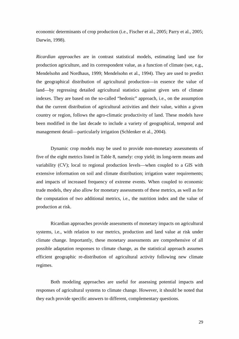
29

economic determinants of crop production (i.e., Fischer et al., 2005; Parry et al., 2005;

Darwin, 1998).

Ricardian approaches are in contrast statistical models, estimating land use for

production agriculture, and its correspondent value, as a function of climate (see, e.g.,

Mendelsohn and Nordhaus, 1999; Mendelsohn et al., 1994). They are used to predict

the geographical distribution of agricultural production—in essence the value of

land—by regressing detailed agricultural statistics against given sets of climate

indexes. They are based on the so-called “hedonic” approach, i.e., on the assumption

that the current distribution of agricultural activities and their value, within a given

country or region, follows the agro-climatic productivity of land. These models have

been modified in the last decade to include a variety of geographical, temporal and

management detail—particularly irrigation (Schlenker et al., 2004).

Dynamic crop models may be used to provide non-monetary assessments of

five of the eight metrics listed in Table 8, namely: crop yield; its long-term means and

variability (CV); local to regional production levels—when coupled to a GIS with

extensive information on soil and climate distribution; irrigation water requirements;

and impacts of increased frequency of extreme events. When coupled to economic

trade models, they also allow for monetary assessments of these metrics, as well as for

the computation of two additional metrics, i.e., the nutrition index and the value of

production at risk.

Ricardian approaches provide assessments of monetary impacts on agricultural

systems, i.e., with relation to our metrics, production and land value at risk under

climate change. Importantly, these monetary assessments are comprehensive of all

possible adaptation responses to climate change, as the statistical approach assumes

efficient geographic re-distribution of agricultural activity following new climate

regimes.

Both modeling approaches are useful for assessing potential impacts and

responses of agricultural systems to climate change. However, it should be noted that

they each provide specific answers to different, complementary questions.

30

Dynamic crop models can be used to successfully identify thresholds of

needed management change; to predict when such thresholds might be reached; and to

assess robustness of specific adaptation strategies. To this end, these models are quite

useful in computing many of the metrics of importance to decision-making, especially

at local to regional level; they provide answers to the following questions: How

vulnerable are given local or regional production systems to climate change? What are

some of the adaptation strategies and what are their effects? Coupled to trade models,

these models can further address questions regarding the linkages between regional

production, trade, food supply, and nutrition levels.

Such models cannot however cover the entire range of possible adaptation

solutions, or the mechanisms necessary for implementation. For these reasons, they

tend to provide overestimates when used to assess overall costs of climate change

impacts. In the vulnerability equation discussed in earlier sections, these models

provide nearly complete information on exposure and sensitivity to exposure of

agricultural systems, and can specify a number of technical aspects of adaptive

capacity.

Ricardian models attempt to compute the overall cost of impacts and thus the system

vulnerability by implicitly considering a wider range of possible adaptation options.

Within this context, they provide first-order, yet static analyses of the economic

vulnerability of regionally or nationally-aggregated production systems. These models

are however of little dynamic value: they cannot provide further insight with regard to

which specific adaptation would actually work, how they would be distributed over a

territory, nor when they should be considered for implementation. In the vulnerability

equation, these models estimate statistically the functional components of exposure

and sensitivity to exposure of production systems, while taking adaptation capacity

out of the equation entirely, by integrating over all possible response strategies.

7. Conclusions

A theoretical framework for climate change impacts and adaptation metrics consists

of the definition and development of metrics needed to quantify and easily

communicate to policy and decision-makers the risks of climate change to agricultural

systems now and in coming decades. The inclusion of stakeholders is a key part of

31

metric development process. With input from stakeholders and experts, we have

developed a set of proposed set of metrics comprised of eight elements for estimating

the short-term (20-30 years) and long-term (80-100 years) impacts of climate change

on agriculture, in monetary and non-monetary terms. This draft metric set may

provide a tool for helping policy and decision–makers evaluate, at regional to national

levels, levels of risk associated with climate change in coming decades, and identify

potential thresholds beyond which significant adaptation of management techniques

need to be implemented. Dynamic crop simulation and Ricardian approaches can

contribute to the calculation of climate change metrics for agriculture. Additional

work is necessary to consult a wider group of stakeholders at national and regional

scales, evaluate methodologies for integrating the different modelling approaches, and

test the resulting framework across a range of agricultural systems, socio-economic

pathways, and climate-change regimes.

32

8. References

Ainsworth, E.A. and Long, S.P., 2005. What have we learned from 15 years of free-air CO2 enrichment (FACE)? A meta-analysis of the responses of photosynthesis, canopy properties and plant production to rising CO2. New Phytologist 165: 351-372.

Bryant, C.R., Smit, B., et al., 2000. Adaptation in Canadian Agriculture to Climatic Variability and change. Climatic Ch. 45(1): 181-201.

Climatic Ch. 45(1): 5-17. Darwin, R., 1998. FARM: A Global Framework for Integrated Land Use/Cover Modeling.

Working Papers in Ecological Economics 9802, Australian National University, Canberra, Australia.

FAO, 2001. The State of Food Insecurity in the World, 2001. Food and Agriculture Organization of the United Nations, Rome, Italy, ISBN 92-5-104628-X.

FAO, 2003. World Agriculture: Towards 2015/1030. A FAO Perspective. Jelle Bruinsma (Ed.) Food and Agricultural Organization of the United Nations, Rome. 432 pp.

Fischer, G., Frohberg, K., Parry, M.L., and Rosenzweig, C., 1996. Impacts of potential climate change on global and regional food production and vulnerability, in E.T. Downing, (Ed.), Climate change and world food security, Springer-Verlag, Berlin, Germany.

Fischer, G., Shah, M., and van Velthuizen, H., 2002. Climate Change and Agricultural Vulnerability, Special Report to the UN World Summit on Sustainable Development, Johannesburg 2002. IIASA, Laxenburg, Austria.

Fischer, G., Shah, M., Tubiello, F.N., and van Velthuizen, H., 2005. Socio-economic and climate change impacts on agriculture: an integrated assessment, 1990-2080. Philosophical Transactionsof the Royal Society B (Phil. Trans. R. Soc. B), 360(1463):2067-2083, DOI: 10.1098/rstb.2005.1744, 29 November 2005. Published online.

Flato, G.M., Boer, G.J., Lee, W.G., McFarlane, N.A., Ramsden, D., Reader, M.C., and Weaver, A.J., 2000. The Canadian Centre for Climate Modelling and Analysis Global Coupled Model and its Climate, Climate Dynamics, 16:451-467.

Gordon, C., Cooper, C.A. Senior, Banks, H., Gregory, J.M., Johns, T.C., Mitchell, J.F.B., and Wood, R.A., 2000. The simulation of SST, sea ice extents and ocean heat transports in a version of the Hadley Centre coupled model without flux adjustments, Climate Dynamics, 16:147-168.

Gordon, H.B., and O'Farrell, S.P., 1997. Transient climate change in the CSIRO coupled model with dynamic sea ice, Monthly Weather Review, 125(5):875–907.

Hirst, A.C., Gordon, H.B., and O’Farrell, S.P., 1997. Response of a coupled ocean-atmosphere model including oceanic eddy-induced advection to anthropogenic CO2 increase, Geophys. Res. Lett., 23(23):3361–3364.

Hitz, S., and Smith, J., 2004. Estimating global impacts of climate change. Glob. Environ. Ch. 14:201-218.

IPCC, 2001a. Climate Change 2001: The Scientific Basis. Contribution of Working Group I to the Third Assessment Report of the Intergovernmental Panel on Climate Change. Cambridge University Press, Cambridge, UK.

IPCC, 2001b. Climate Change 2001: Impacts, Adaptation, and Vulnerability. Contribution of Working Group II to the Third Assessment Report of the Intergovernmental Panel on Climate Change. Cambridge University Press, Cambridge, UK.

Jablonski, L.M., Wang, X., Curtis, P.S., 2002. Plant reproduction under elevated CO2 conditions: A meta-analysis of reports on 79 crop and wild species. New Phytologist 156 (1): 9-26.

Jones, R.N., 2003. Managing climate change risks. OECD ENV/EPOC/GSP, 37pg. OECD, Paris France.

Jones, R.N., 2001. An environmental risk assessment/management framework for climate change impact assessments. Nat. Hazards 23: 197-230.

33

Kane, S.M., and Shogren, J.F., 2000. Linking Adaptation and Mitigation in Climate Change Policy. Climatic Ch. 45(1): 72-102.

Kane, S.M., and Yohe, G.W., 2000. Societal adaptation to climate variability and change: An introduction. Climatic Ch. 45(1): 1-4.

Kates, R.W., 2000. Cautionary Tales: Adaptation and the Global Poor. Kimball, B.A., Kobayashi, K., Bindi, M., 2002. Responses of agricultural crops to free-air

CO2 enrichment. Adv. Agron. 77: 293-368. Mendelsohn, R., and Nordhaus, W., 1999. The impact of climate on agriculture: a Ricardian

approach: A reply. Amer. Econ. Rev. 89(4): 1046-48. Mendelsohn, R., Nordhaus, W. and Shaw, D. 1994. The impact of climate on agriculture: a

Ricardian approach. Amer. Econ. Rev. 84: 753-771. Millennium Ecosystem Assessment, 2005. Ecosystems and human well-being: Synthesis.

Washington, DC: Island Press. Nakicenovic, N., and Swart, R. (eds.), 2000. Emissions Scenarios, 2000, Special Report of the

Intergovernmental Panel on Climate Change, Cambridge University Press, UK. pp 570 New, M.G., Hulme, M., and Jones, P.D., 1998. Representing 20th century space-time climate

variability, in Development of a 1961-1990 mean monthly terrestrial climatology, J. Climate, available at http://www.cru.uea.ac.uk/link.

Oberhuber, J.M., 1993. Simulation of the Atlantic circulation with a coupled sea-ice mixed layer-isopycnal general circulation model. Part I: Model description. J. Phys. Oceanogr., 13, 808-829.

Parry, M., Rosenzweig, C., and Livermore, M., 2005. Climate change, global food supply and risk of hunger. Phil. Trans. R. Soc. B 360: 2125–2138.

Parry, M.L., N.W.Arnell, A.J. McMichael, R.J. Nicholls, P. Martens, R.S. Kovats, M.T.J. Livermore, C. Rosenzweig, A. Iglesias, G. Fischer, 2001. Millions at Risk: Defining Critical Climate Change Threats and Targets. Global Environmental Change, 11:181-183.

Parry, M.L., Rosenzweig, C., Iglesias, A., Fischer, G., and Livermore, M.T.J., 1999. Climate change and world food security: A new assessment, Global Environmental Change, 9:51-67.

Parry, M.L., Rosenzweig, C., Iglesias, A., Livermore, M., Fischer, G., 2004. Effects of climate change on global food production under SRES emissions and socio-economic scenarios. Global Environmental Change 14: 53–67.

Pope, V.D., Gallani, M.L., Rowntree, P.R., and Stratton, R.A., 2000. The impact of new physical parametrizations in the Hadley Centre climate model—HadAM3, Climate Dynamics, 16:123-146.

Reilly, J., and Schimmelpfennig, D., 2000. Irreversibility, Uncertainty, and Learning: Portraits of Adaptation to Long-Term Climate Change. Climatic Ch. 45(1): 253-278.

Reilly, J., Tubiello,F.N., McCarl, B., and Melillo, J., 2001. Climate change and agriculture in the United States, in: Melillo, J., Janetos, G., and Karl, T., (Eds), Climate Change Impacts on the United States: Foundation, USGCRP. Cambridge University Press, Cambridge, UK. 612 pp.

Roeckner, E., Arpe, K., Bengtsson, L., Brinkop, S., Dümenil, L., Esch, M., Kirk, E., Lunkeit, F., Ponater, M., Rockel, B., Suasen, R., Schlese, U., Schubert, S. and Windelband, M., 1992. Simulation of the present-day climate with the ECHAM 4 model: impact of model physics and resolution. Max-Planck Institute for Meteorology, Report No. 93, Hamburg, Germany, 171 pp.

Roeckner, E., Arpe, K., Bengtsson, L., Christoph, M., Claussen, M., Dümenil, L., Esch, M., Giorgetta, M., Schlese, U., and Schluzweida, U., 1996. The atmospheric general circulation model ECHAM-4: model description and simulation of present-day climate. Max-Planck Institute for Meteorology, Report No. 218, Hamburg, Germany, 90 pp.

Rosenzweig, C. and Parry, M. L, 1994. Impacts of climate change on world food supply. Nature, 367: 133-138.

Rosenzweig, C., Allen, L.H.Jr., Harper, L.A., Hollinger, S.e., and Jones, J.W. (Eds), 1995. Climate Change and Agriculture: Analysis of Potential International Impacts, ASA Special Publication No. 59, Madison, WI.

34

Rosenzweig, C., and Tubiello, F.N., 2006. Interactions of adaptation and mitigation strategies in agriculture. Mitig. Adapt. Strat. Clim. Ch. In press.

Rosenzweig, C., and Tubiello, F.N., 2006. Interactions of adaptation and mitigation strategies in agriculture. Mitigation and Adaptation Strategies for Climate Change. In press.

Rosenzweig, C., F.N. Tubiello, R.A. Goldberg, E. Mills, J. Bloomfield, 2002. Increased crop damage in the U.S. from excess precipitation under climate change, Global Env. Change, 12: 197-202.

Schneider, S.H., Easterling, W.E., and Mearns, L.O., 2000. Adaptation: Sensitivity to Natural Variability, Agent Assumptions and Dynamic Climate Changes. Climatic Ch. 45(1):203-221.

Smit, B., Burton, I., Klein, R.J.T., et al., 2000. An Anatomy of Adaptation to Climate Change and Variability. Climatic Ch. 45(1): 223-251.

Tsuji, G.Y., G. Uehara, and S. Balas (Eds.). 1994. DSSAT v3. University of Hawaii, Honolulu, Hawaii.

Tubiello, F.N., Jagtap, S., Rosenzweig, C., Goldberg, R., and Jones, J.W., 2002. Effects of climate change on U.S. crop production from the National Assessment. Simulation results using two different GCM scenarios. Part I: Wheat, Potato, Corn, and Citrus, Climate Res. 20(3), 259-270.

Tubiello,F.N. and Ewert, F., 2002. Modeling the effects of elevated CO2 on crop growth and yield: A review. Eur. J. Agr. 18(1-2),57-74.

UN Millenium Project, 2005. Investing in Development. A practical plan to achieve the Millenium Development Goals. Report to the UN Secretary General. ISBN 1-884707-217-1. New York.

Washington, W.M., Weatherly, J.W., Meehl, G.A., Semtner, A.J., Jr., Bettge, T.W., Craig, A.P., Strand, W.G., Jr., Arblaster, J.M., Wayland, V.B., James, R., Zhang, Y., 2000. Parallel climate model (PCM) control and transient simulations, Climate Dynamics, 16(10/11):755-774.

Watson, R.T., Noble, I.R., Bolin, B., Ravindranath, N. H., Verardo D. J., and Dokken, D. J., 2000. IPCC Special Reports. Land Use, Land-Use Change, and Forestry. Cambridge University Press, Cambridge, 324 pp.

Williams, J.R. 1995. The EPIC Model. In: V.P. Singh (Ed.) Computer models of watershed hydrology. Water Resources Publications. Highlands Ranch, Colorado.

World Bank, 2005. Managing agricultural production risk. Report No. 32727-GLB. The International Bank for Reconstruction and Development/The World Bank, Washington DC.

35

Figures Figure 1. Socio-economic SRES scenarios determine both climatic and market conditions in integrated agro-economic assessments. Climatic impacts on agricultural production –computed with crop models— are used as inputs to agricultural economics and trade models to determine overall impacts on world food systems. Figure 2. GCM-predicted mean annual temperature change over land, as a function of corresponding CO2 concentrations (a proxy for time from1990 to 2080) and against GCM- predicted mean annual precipitation change. Graphs show results for all 14 scenarios considered in this study, computed for all land in a) Developed world; b) Developing world. Figure 3. Changes in potentially attainable cereal production predicted under different GCM climate change scenarios, vs. global mean temperature change. Projections are for either current cultivated land (right), or all available under future climates (left), and pooled into developed (top) and developing (bottom) countries. Results are expressed against a scaled index of production set at 100 in 1990.

36

FIGURE 1

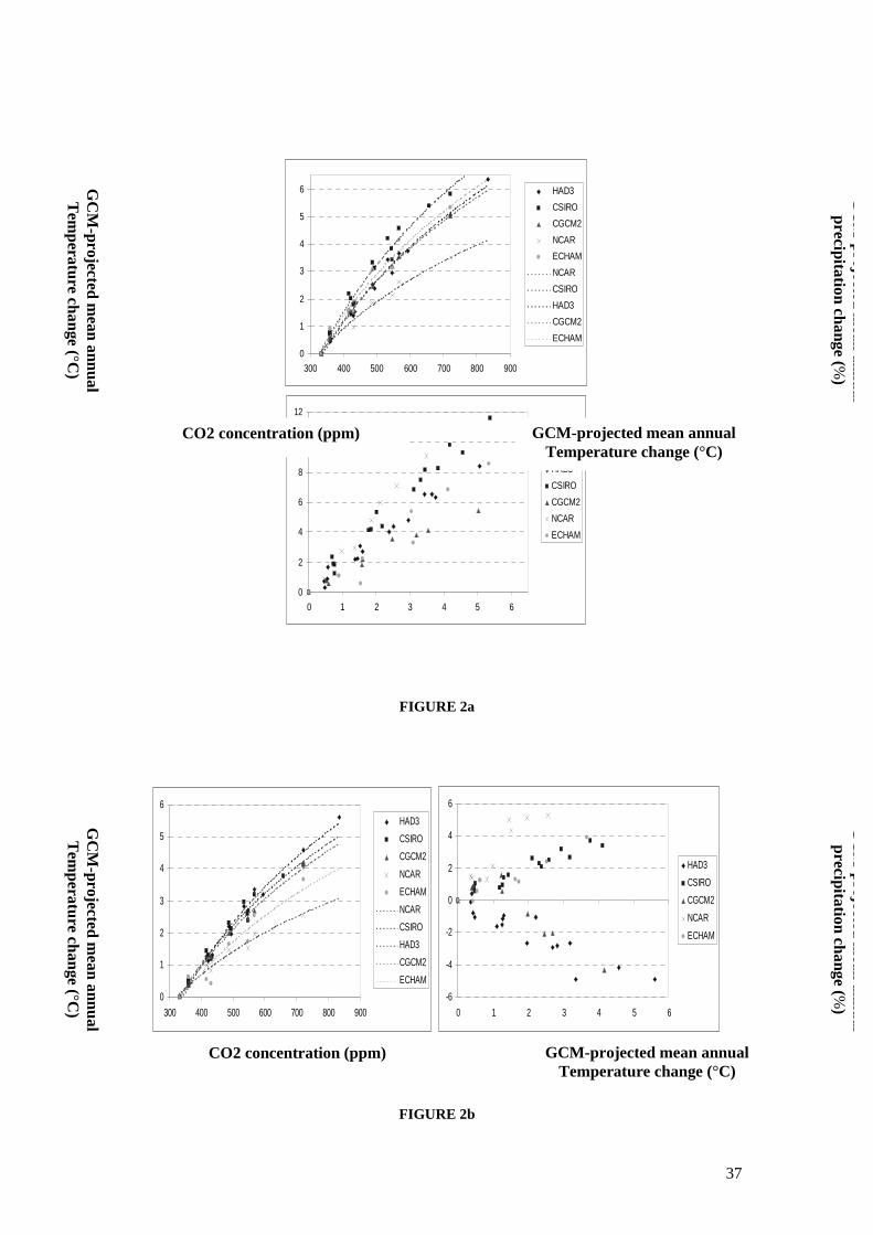
37

0

1

2

3

4

5

6

300 400 500 600 700 800 900

HAD3

CSIRO

CGCM2

NCAR

ECHAM

NCAR

CSIRO

HAD3

CGCM2

ECHAM

0

2

4

6

8

10

12

0 1 2 3 4 5 6

HAD3

CSIRO

CGCM2

NCAR

ECHAM

FIGURE 2a

0

1

2

3

4

5

6

300 400 500 600 700 800 900

HAD3

CSIRO

CGCM2

NCAR

ECHAM

NCAR

CSIRO

HAD3

CGCM2

ECHAM

-6

-4

-2

0

2

4

6

0 1 2 3 4 5 6

HAD3

CSIRO

CGCM2

NCAR

ECHAM

FIGURE 2b

CO2 concentration (ppm) GCM-projected mean annual Temperature change (°C)

G

CM

-projected mean annual

Tem

perature change (°C)

GC

M-projected m

ean annual precipitation change (%

)

CO2 concentration (ppm) GCM-projected mean annual Temperature change (°C)

GC

M-projected m

ean annual T

emperature change (°C

)

GC

M-projected m

ean annual precipitation change (%

)

38

39

Developed, all land Developed, current cultivated land

100

110

120

130

140

150

0 1 2 3 4 5

Tempera

HAD3CSIROCGCMNCARHAD3CGCMNCARCSIRO

90

100

110

120

130

0 1 2 3 4 5

Temper

HAD3CSIROCGCMNCARHAD3NCARCGCMCSIRO

Developing, all land Developing, current cultivated land

95

100

105

110

115

0 1 2 3 4 5

Tempera

HAD3CSIROCGCMNCARHAD3CGCMNCARCSIRO

95

100

105

110

115

0 1 2 3 4 5

Temper

HAD3CSIRCGCMNCARHAD3NCARCGCMCSIR

FIGURE 3

40

Appendix A. Workshop Report and Case Study Summary

Climate Change Impacts and Adaptation Metrics (CCIAM) Workshop

NASA Goddard Institute of Space Studies

June 5-6, 2006

1. Attendees

Walter Baethgen IRI, Columbia University/ IFDC, USA and Uruguay

Livia Bizik Slovak Academy of Sciences/ University of British Columbia, Slovakia and Canada

Vittorio Canuto NASA-GISS Marcello Donatelli ISCI Bologna, Italy PierPaolo Duce University of Sassari, Italy Bill Easterling Pennsylvania State University Richard Goldberg Columbia University, USA Daniel Hillel Columbia University, USA Alexander Lotsch Community Risk Management Group, the World Bank Cynthia Rosenzweig NASA-GISS, USA Wolfram Schlenker Columbia University, USA Richard Snyder UC Davis, USA Donatella Spano University of Sassari, Italy

Andrea Taramelli Columbia University/ University of Perugia, USA and Italy

Francesco Tubiello Columbia University, USA Gary Yohe Wesleyan University, USA Francesco Zecca Ministry of Agriculture and Forestry, Italy

The workshop was structured in three parts: Presentations followed by discussion,

inputs for metrics development from break-out group discussion sessions, and

feedback on the draft questionnaire. Key ideas from the workshop are summarized

below.

2. Day One - Monday 5th June

Cynthia Rosenzweig and Francesco Tubiello introduced the overall aims of the

project and the purpose of the workshop. Rosenzweig shared with attendees the

recent progress in developing a global map showing observed changes worldwide in

agriculture due to observed climate change trends. This was followed by presentations

on draft metrics from biophysical and socio-economic perspectives, break-out group

discussions on CCIAM development and use, and regional case studies.

41

Lessons from Case Studies

During this session, Livia Bizik, Donatella Spano, Walter Baethgen and Bill

Easterling shared their findings from various case studies with suggestions towards

the development of useful metrics for agriculture.

Livia Bizik identified the socio-economic transformations of transition countries as

drivers of negative changes that occurred in agricultural sector in the region. Bizik

used Slovakia, Poland and Ukraine as examples. Major changes occurred in terms of

private land ownership, which led to increased fragmentation of land, in these

countries since 1990. Land abandonment is identified as another threat to agricultural

system. There are significant changes in the level of institutional development in the

region that can play positive role in climate change adaptation.

Donatella Spano reported results from studies conducted in Sardinia and Emilia-

Romagna regarding the impact of climate change on Italian agriculture. The main

objectives were to develop a methodology for assessing climatic risk based on

bioclimatic indexes, to evaluate the potential effects of climatic variations on

agriculture and to obtain maps of climatic risk for agriculture based on past and future

climatic variability. Lessons from this study includes: Due to climate variability in

the Mediterranean region, metric based on observed trends is not very useful in this

region and several decades of data is needed to determine the climate change impacts

on agricultural production. The impacts are heterogeneous. In Sardina, precipitation

was the main factor and in Emilia Romagna, both temperature and precipitation were

important in determining climatic effect on Land Capability for Agriculture.

In Walter Baethgen’s study, climate and crop yield and price have been used as

observed trend metrics. The studies are conducted by AIACC—a GEF funded

organization—in pampas of Argentina, Brazil and Uruguay. Using data 1930-2000,

these studies show increased precipitation, decreased max temperature, increased min

temperature and shorter and milder frost seasons that would positively impact land

use changes but incidences of diseases would be higher.

42

Bill Easterling is in favor of looking at thermal time calculating degree days and heat

stress days. Kendall-Thiel Regression calculated thermal time that measures heat

stress days and shows upward trend. Annual heat stress day shows downward trend.

Economic Perspectives

During this session, Alexander Lotsch and Wolfram Schlenker discussed the

economic components of adaptation metrics.

Alexander Lotsch explained how and why index-based insurance model works. The

Community Risk Management Group model uses the change in cropland patterns as a

function of climate change. Cropland density model for Africa projects that most of

the cropland will be lost over the next 30 years. CRMG agenda for new business

model for risk management includes: insure weather and disaster risks for developing

countries; target most vulnerable populations; risk transfer; partner with major re-

insurers to ensure sustainability; enable the poor and supporting institutions to adapt.

At first, the pilot program began with a couple of hundred insurers in India, and then a

couple of thousand farmers were insured. World Bank develops the product and then

sells the product to insurance agency. Insurance company evaluates the data. This

kind of product can be traded as derivatives.

In Wolfram Schlenker’s analysis, hedonic studies capture adaptations on behalf of

farmers. Using panel data of corn, soybeans, and cotton yields has large negative

effect of heat waves and support for the concept of degree days. The bottom line is

the non-linearity between weather and crop yield. East of the US shows losses in the

aggregate, no technological progress in heat resistance in last 55 years and limited

potential for adaptation. Mean shifts versus variance increases. In hedonic study,

losses are lower with adaptation and results are comparable between models. Water

rights are very important in the U.S. West.

Mediterranean Marginal Environments

Marcello Donatelli shared the findings of a paper that he coauthored with Cynthia

Rosenzweig and Francesco Tubiello. The objectives of this work are to evaluate the

impact of climate change scenarios on cropping systems, to develop adaptation

strategies to alleviate the negative outcomes of such scenarios and to highlight major

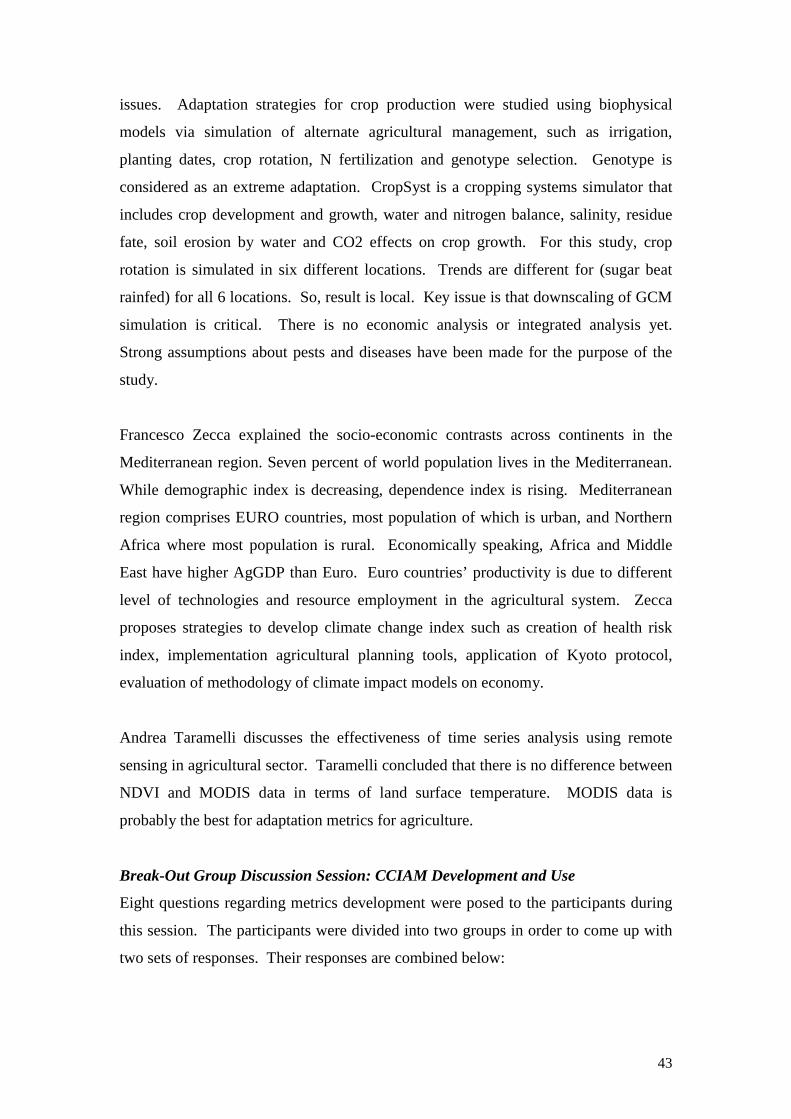
43

issues. Adaptation strategies for crop production were studied using biophysical

models via simulation of alternate agricultural management, such as irrigation,

planting dates, crop rotation, N fertilization and genotype selection. Genotype is

considered as an extreme adaptation. CropSyst is a cropping systems simulator that

includes crop development and growth, water and nitrogen balance, salinity, residue

fate, soil erosion by water and CO2 effects on crop growth. For this study, crop

rotation is simulated in six different locations. Trends are different for (sugar beat

rainfed) for all 6 locations. So, result is local. Key issue is that downscaling of GCM

simulation is critical. There is no economic analysis or integrated analysis yet.

Strong assumptions about pests and diseases have been made for the purpose of the

study.

Francesco Zecca explained the socio-economic contrasts across continents in the

Mediterranean region. Seven percent of world population lives in the Mediterranean.

While demographic index is decreasing, dependence index is rising. Mediterranean

region comprises EURO countries, most population of which is urban, and Northern

Africa where most population is rural. Economically speaking, Africa and Middle

East have higher AgGDP than Euro. Euro countries’ productivity is due to different

level of technologies and resource employment in the agricultural system. Zecca

proposes strategies to develop climate change index such as creation of health risk

index, implementation agricultural planning tools, application of Kyoto protocol,

evaluation of methodology of climate impact models on economy.

Andrea Taramelli discusses the effectiveness of time series analysis using remote

sensing in agricultural sector. Taramelli concluded that there is no difference between

NDVI and MODIS data in terms of land surface temperature. MODIS data is

probably the best for adaptation metrics for agriculture.

Break-Out Group Discussion Session: CCIAM Development and Use

Eight questions regarding metrics development were posed to the participants during

this session. The participants were divided into two groups in order to come up with

two sets of responses. Their responses are combined below:

44

1. Who are the stakeholders for climate change and agriculture metrics? What

is the key spectrum of scales?

Initially, stakeholders at the national level should be contacted, and finance ministries

are needed to be contacted as well. In general, if the metric needs to provide a general

guide about the capacities and needs to address climate change and agriculture with

regard to both biophysical and socio-economic determinants, the stakeholders should

be governments of the countries. The governments of the countries will be able to

utilize the generic information from the metrics to strengthen the weakest part of their

adaptive capacities and also take it into account in designing future policies and

incentives for certain agricultural practises. In terms of the spectrum of scales,

national agricultural planners can help setting the framework and regional planners

can provide local data.

2. What are the stakeholders’ needs at the different scales? Do needs differ

among groups?

Stakeholders need not only hazard assessment, but also socio-economic metrics for

quantifying the resiliency of the system. Needs for metrics differ among different

groups.

3. What overall framework is needed?

• Risk management and risk analysis approaches can be used as frameworks for

metrics development, and adaptation and mitigation can be seen as

complements.

• Long term policy perspective should be taken into consideration.

• It is important to define risk assessment and risk management

• Emphasize financing component of climate change problem.

• In terms of impact, cost and benefit are important.

• Make reference to existing indicators of agricultural production systems

• Identify ways to convince developing countries to adapt to climate change?

• Provide direct support for adaptation (primary task is to make clear

comparison between adaptation benefits in 20-30 years and lack there of).

45

• Identify ways for agricultural management adaptation.

• What do we keep track of to make decisions? Annual basis? Within a trend,

what are the thresholds to keep track of?

• Frame climate change as a constraint of future development.

• Considerations to climate change impacts are presented as an important

element to improve inequality at the global and country level (strong value-

basis).

• Focus on reducing vulnerability exaggerated by climate change impacts on

food systems at the global level

• Support agricultural development that do not deteriorate the environment

• Develop sets of metrics as exposures, metrics to sensibility to exposures, and

metrics to adaptive capacity.

4. What specific metrics are needed for the different groups? (Global/regional

climate and agro-climate indices for climate change risk and thresholds)

It is important to identify the affected sectors, crops and specific stresses that they are

being exposed to. Thresholds should be specific to the sectors, crops and stresses and

should include prices.

Temperature and precipitation are universally important across different groups.

Dependent index would be useful for Euro region, while number of people at risk of

starvation is more appropriate for developing countries. Rain fed crop is important

because it directly depends upon availability of water resources. Level of irrigation

and health could be considered as vulnerability indices. More coverage for spatial

data is needed.

5. What timeframes should be considered? Past/Present/Future (time-slices?)

Agricultural decisions are focused in the short-term, so this should be the operational

focus. Data from the past is useful for calibration, and current conditions are essential

to establish a baseline. Long term data can be used primarily to understand climate

change and to invest on structural changes looking at 2050, for example. Different

time frame is needed for sensitive areas such as Mediterranean. Historical land use

46

study is important for transition countries. Metrics should be standardized to baseline

period (30 years). 50 years of time series data would be appropriate for national level

approach.

Metrics need to reflect on changes occurring in the countries with regards to

adaptation needs and potentials. It requires of setting up baseline and moving

backward and forward to monitor the change. In this way metric will prove dynamic

information about the change, however it won’t be able to reflect on the processes

going on in the countries. Therefore, the idea of case studies is highly relevant in

order to improve the interpretation of the country-level data and also to address

important regional and local synergies and trade-offs linking agricultural change with

other sectors and with local livelihood.

6. How should socio-economic pathways be handled?

It may be difficult to apply socio-economic threshold concepts at the local level, e.g.,

frequencies of exceeding social-economic thresholds may be difficult to quantify. For

example, it may be difficult to anticipate when resource use exceeds the supply, or to

determine the thresholds for the price of maize or cost of water. Multiplicity of

overlapping thresholds may also be problematic.Mitigation strategies for reduction of

GHGs need to be factored in.

7. How should adaptation levels be handled? How can we bring the biophysical

and economic approaches together?

Climatic consequences can be enumerated in economic terms. However, it is difficult

at times to give economic value to natural resources. Different evaluation should be

considered given different stakeholders. Multi-criteria analysis is useful, but there is

uncertainty in making operational use of analysis. AIACC scientists can be requested

to identify ten aspects that that they learned and that can be synthesized and

communicated across regions. Agricultural data would be more relevant as a

vulnerability index. Africans need more support. International academic and

development institutions such as IRI and DFID have been providing funds for

developing knowledge base in developing countries.

47

8. How should climate change metrics be communicated?

Understanding the system before proposing adaptation options is important.

Currently people have different perceptions of risks. Response strategies to climate

extremes should be improved. To increase awareness, internet can be very effective.

Raising awareness of extension services as access way to farmers is important.

Uncertainty elements should be communicated to the policy makers. Biophysical

indices are better for the scientific community and socio-economic indices are the key

to get the message across in public policy arena.

3. Day Two - Tuesday 6th June

Day Two was comprised of reporting and further discussion regarding CCIAM

development and use between the two break-out groups. The participants also shared

their feedback on the appropriateness of the draft questionnaire for stakeholders.

Reports from Brfeak-out Group Discussions: CCIAM Development and Use

(Continued from Day One)

Main points:

• Data need not be equated with the index at the beginning. Indices should be

developed first, and then more input from the stakeholders can be requested to

improve them.

• Indices should be feasible and good quality spatial data should be available for

developing these indices.

• Observation system of systems is required since error bars are too high for

climate change and for insurance product, sound data is needed. Remote

sensing is used for CRMG model as ancillary.

48

• For the adaptation side and on the metric side, insurance and creating safety

net are important.

• Crop simulation model can integrate human and financial resources with crude

soil and water balance.

• Stakeholders should be able to relate to the metrics. So, cruder metrics would

be better in order to make them involved. Stakeholders from developed and

developing countries need to be involved in the process of developing region

specific metrics. There is a mismatch between the probabilistic climate

forecast and stakeholders’ ability to respond in the developing countries. In

order to have the policy makers on board, socio-economic indices should be

give special attention to address adaptation.

• Some indices are inflated by technical consideration.

• Some of the adaptation capacity depends on a country’s endowment of

resources. Definition of exposure, sensitivity and vulnerability should be

compartmentalized. The definitions are completely different in different

institutions.

Feedback for Draft Questionnaire

For reference, the questionnaire is included in Appendix B. The participants

suggested that figures with key trends of agricultural system and/or some economic

indicators or coping strategy diagram or world map with climate change on it could be

usefully added to the questionnaire. Uncertainty caveats should also be mentioned.

Question 2 is not appropriate for CCIAM. Question 3 has to have a timeframe.

Multiple choices with Other option would be better for Question 3.

The participants recommended that a possible modification for Question 6 can be to

ask policy makers/ farmers at what point they would intervene. One way to determine

threshold level is to work along a continuum and identify a cut off point. Different

threshold has different set of sensitivity. Stakeholders’ workshop is a way to find out

what the stakeholders think is critical threshold and their response to risk

management. Other possible questions to the stakeholders could be “what could you

49

do in the anticipation of approaching certain threshold in ex-ante period, and in case

you have not prepared, what would you do in ex-post period?”

According to the workshop participants, targeted interviews with few important

stakeholders may be helpful at the initial level. Lists of bio-physical indicators in

order to describe the problem and socio-economic indicators in order to communicate

the setbacks are important. Scenarios will useful for scientists. They can be used in

developing adaptation scenarios as well. Monitoring and evaluation criteria have to

be developed at the beginning of the CCIAM design process.

4. Main Outcomes

During the final session, Cynthia Rosenzweig and Francesco Tubiello wrapped up the

workshop reiterating the take-away points and requested each participant to share

their final thoughts. Key ideas for metrics development are summarized in Table W1

and ithe following:

• Importance of the process:

o Engage stakeholder from the beginning

o Plan an evaluation process from the beginning.

o Keep it realistic, manage expectations. Emphasize so as to not raise

expectation that you’d deliver the metrics, rather on the process of

developing metrics.

o Understand the criticality of threshold when they exceed something.

o Metrics should be as simple as possible, but not too simple to be

useless. Being mindful of the users will be important.

o Importance of raw data part—levels of processes should be from

simple to complex.

o Understanding of exposure, sensitivity and vulnerability to climate

change is crucial. Consideration of mitigation and adaptive capacity

sides is also important.

o Call vulnerability resilience--constructive part.

• Metrics development

50

o Include the uncertainty

o Include observed changes and some projection in the metrics.

o Differential approaches for different location.

o Revisit the models. Models are disjointed now.

o CO2 fertilization effect.

o More questions about economic impact and indicators.

Table W1. Suggestions for CCIAM metrics development. Categories Vulnerability

criteria Indices Processes

Climate Soil Crop calendar Water storage

Biophysical Exposure

Biomass/ Production Crop insurance programs Trade flow (isolation) % agriculture sector in subsistence (e.g., health, education)

Socio-economic Sensitivity

% agriculture sector in poverty and inequality, (e.g., wages) Technological change % arable land currently in use % rainfed crops/ irrigated crops

Agricultural Adaptive capacity

Education

Kyoto commitment capacity

Mitigation

Carbon sequestration: CDM projects in place

• Data collection • Processing • Time series • Critical thresholds • Climate change

scenarios • Testing/evaluation • Stakeholder

involvement • Developed/

developing countries

5. Summary of Case Studies

51

Case studies provided an opportunity to further develop effective metrics.

Representatives at the workshop focused on production systems in:

1) US Midwest;

2) Southeast South America;

3) Slovakia and Ukraine; and

4) 4) Mediterranean/Italy.

Examples of information were gathered via interactions with stakeholders at the

workshop relative to the classification scheme we proposed above, leading to the

compilation of several tables to be used for analysis. For instance, with reference to

Table 2, simple initial screening could be performed:

Regions 1 and 4 are in Developed Countries, Regions 2 and 3 in Developing

Countries.

All four regions have stable climate with specific variability issues: flooding and

drought impact crop yields in all these regions.

Inputs of nitrogen are high in Regions 1, 2 and 4 (minimal yield gaps), while most

production in Region 3 is rainfed and at low-nitrogen input levels, with substantial

gaps between attainable and actual yields.

Variability of production is low in Region 1, medium in Region 2, and high in

Regions 3 and 4.

Similarly, production technology is advanced in Regions 1 and 4, medium in Region 2

and low in Region 3.

Land-use structure is an important assessor of vulnerability/adaptation capacity. In

Regions 1 and 2 the main production unit is in the order of 100 ha; Regions 2 and 4

have smaller units, 10-50 ha; while 1-10 ha is the common plot size in Region 3.

52

Draft Questionnaire

“Improving Methodologies to Assess the Benefits of Policies to Address Climate Change Impacts on Agriculture”

QUESTIONNAIRE

1.1 SECTION 1 – Professional details (Please note: use the tab key to navigate the questionnaire; boxes will expand as information is added) 1. Please give your profession and nationality 2. Into which categories does your organisation belong? Type Level Governmental - management Local Governmental - policy Regional Charitable organisation National Research – university based International Research – other Private company Other: (Please define)

53

1.2 SECTION 2 – Reduction in Crop Yield Error!(Add Figure)

The above figure illustrates plausible projected levels of crop yield for the next 500 years from a range of predictive models. The large range reflects uncertainties in future emissions of greenhouse gasses and crop yield response to the resulting global warming. 1. Taking a professional perspective, what issues and challenges might these possible changes raise for your organisation? 2. Which of the four (may have more or fewer curves) curves (if any) would form the basis for any strategic planning decisions? 3. How far into the future would these scenario(s) be considered as part of any planning decision?

54

4. Which indicator(s) would be most beneficial?

(i) to gauge the implications of crop failure for your organisation e.g. area at risk; people at risk; heritage/culture at risk, risk of increased frequency of extreme events such flood, droughts, etc. (ii) for communication of these implications to colleagues and the wider public e.g., number of tons of crop lost per hectare, tons of crop produced per year, long term standard deviation from mean crop yield over mean yield (%), etc.

5. Do you find these scenarios useful for your organisation?

6. Would an alternative approach based on system sensitivity be useful? You might define a value at which the system(s) you are managing would be significantly affected by the magnitude or rate of change in crop yield. Would establishing such threshold(s) and their timing using the figure be a useful alternative methodology? For example, (i) given a design specification of agricultural practice, identification of when the frequency of crop failure would become unacceptable would indicate the time span over which alternative management regimes or investment programme would need to be prepared (ii) having decided the point at which agricultural ecosystem starts to significantly decline, when this point is likely to be reached. If yes, please expand on the issues that are raised.

7. Any other comments? Thank you for participating in this research. If you require further information or have any questions regarding this research, please do not hesitate to contact Cynthia Rosenzweig at crosenzweig@giss.nasa.gov and/or francesco tubiello at franci@giss.nasa.gov. Please note: all of your answers will be treated in accordance with NASA-GISS’s code of ethical research, which guarantees the confidentiality, anonymity and protection of all research participants. Thank you.