Developing a Power Query Solution in Excel...

Power BI

►Lab 03

Developing a Power Query

Solution in Excel 2013

Jump to the Lab Overview

© Copyright 2014 Microsoft Corporation. All rights reserved.

Terms of Use

© 2014 Microsoft Corporation. All rights reserved.

Information in this document, including URL and other Internet Web site references, is subject to change

without notice. Unless otherwise noted, the companies, organizations, products, domain names, e-mail

addresses, logos, people, places, and events depicted herein are fictitious, and no association with any real

company, organization, product, domain name, e-mail address, logo, person, place, or event is intended

or should be inferred. Complying with all applicable copyright laws is the responsibility of the user.

Without limiting the rights under copyright, no part of this document may be reproduced, stored in or

introduced into a retrieval system, or transmitted in any form or by any means (electronic, mechanical,

photocopying, recording, or otherwise), or for any purpose, without the express written permission of

Microsoft Corporation.

For more information, see Microsoft Copyright Permissions at http://www.microsoft.com/permission

Microsoft may have patents, patent applications, trademarks, copyrights, or other intellectual property

rights covering subject matter in this document. Except as expressly provided in any written license

agreement from Microsoft, the furnishing of this document does not give you any license to these

patents, trademarks, copyrights, or other intellectual property.

The Microsoft company name and Microsoft products mentioned herein may be either registered

trademarks or trademarks of Microsoft Corporation in the United States and/or other countries. The

names of actual companies and products mentioned herein may be the trademarks of their respective

owners.

This document reflects current views and assumptions as of the date of development and is subject

to change. Actual and future results and trends may differ materially from any forward-looking

statements. Microsoft assumes no responsibility for errors or omissions in the materials.

THIS DOCUMENT IS FOR INFORMATIONAL AND TRAINING PURPOSES ONLY AND IS PROVIDED

"AS IS" WITHOUT WARRANTY OF ANY KIND, WHETHER EXPRESS OR IMPLIED, INCLUDING BUT

NOT LIMITED TO THE IMPLIED WARRANTIES OF MERCHANTABILITY, FITNESS FOR A PARTICULAR

PURPOSE, AND NON-INFRINGEMENT.

http://www.microsoft.com/permission


Contents

TERMS OF USE ............................................................................................................................... 1

CONTENTS ..................................................................................................................................... 3

ABOUT THE AUTHOR .................................................................................................................... 4

DOCUMENT REVISIONS ................................................................................................................ 4

LAB OVERVIEW .............................................................................................................................. 5

EXERCISE 1: DEVELOPING A POWER QUERY SOLUTION ........................................................... 7

Task 1 – Opening and Exploring the Excel Workbook ................................................................................................ 7

Task 2 – Enabling the Power Pivot Add-in ....................................................................................................................... 8

Task 3 – Exploring the Power Pivot Data Model ............................................................................................................ 9

Task 4 – Exploring Sales Target Data Extracts................................................................................................................. 9

Task 5 – Creating a Power Query Query ........................................................................................................................ 11

Task 6 – Creating a Power Query Function ................................................................................................................... 20

Task 7 – Invoking the Power Query Function and Combining Queries ............................................................. 24

Task 8 – Organizing the Workbook Queries ................................................................................................................ 28

EXERCISE 2: INTEGRATING THE SOLUTION WITH THE WORKBOOK DATA MODEL ........... 30

Task 1 – Exploring the Power Pivot Data Model ......................................................................................................... 30

Task 2 – Developing the Data Model Enhancements ............................................................................................... 31

Task 3 – Creating a PivotTable Report ............................................................................................................................ 38

Task 4 – Finishing Up ............................................................................................................................................................. 40

SUMMARY .................................................................................................................................... 40


About the Author

This lab was designed and written by Peter Myers.

Peter Myers has worked with Microsoft database and development products since

1997. Today, he specializes in all Microsoft BI products and provides mentoring,

technical training, and education content authoring for SQL Server, Office, and

SharePoint. Peter has a broad business background supported by a bachelor’s

degree in applied economics and accounting, and he extends this with solid experience backed

by current MCSE and MCT certifications. He has been a SQL Server MVP since 2007.

Document Revisions

# Date Author Comments

0 24-AUG-2014 Peter Myers Initial release

1 04-OCT-2014 Peter Myers Updated for Power Query v2.16.3785.242

http://www.linkedin.com/in/peterjsmyers


Lab Overview

Introduction

Note: This lab is the third in a series of seven labs, which explore self-service BI with Excel 2013

and Office 365 Power BI. If you plan to complete all of the labs, we recommend that you

complete them in the order in which they were designed, although the labs can be completed

in any order you choose.

This lab was produced by using the Microsoft Power Query for Excel version 2.16.3785.242

published 29 September, 2014.

In this lab, you will use Power Query to extend the Power Pivot workbook created in Lab 02 with

additional data to enable the performance monitoring of sales against sales target. The sales

target data by state will be sourced from CSV and XML data extract files.

The goal of this lab is to query and transform the data extract files by using Power Query, and

then to add the query to the existing workbook data model (created in Lab 01). Once added,

the query – now in the form of data model table – will be used to extend the data model with

new calculated fields and a key performance indicator (KPI) to enable sales performance

monitoring.

Finally, you will create a PivotTable report. The final report will look like the following.

Figure 1

Previewing the PivotTable Report

http://www.microsoft.com/en-us/download/details.aspx?id=39379

http://www.microsoft.com/en-us/download/details.aspx?id=39379


Objectives

The objectives of this exercise are to:

Query and transform CSV and XML data by using Power Query

Extend an existing workbook data model with a Power Query query result

Enrich the workbook data model with new calculated fields and a KPI

Create a PivotTable report

Exercises

This hands-on lab comprises the following exercise:

1. Developing a Power Query Solution

2. Integrating the Solution with the Workbook Data Model

Estimated time to complete this lab: 60 minutes


Exercise 1: Developing a Power Query Solution

In this exercise, you will use Power Query to extend the Power Pivot workbook created in Lab 02

with additional data to enable the performance monitoring of sales against sales target. Sales

target data by state will be sourced from CSV and XML data extract files.

Task 1 – Opening and Exploring the Excel Workbook

In this task, you will open an existing Excel workbook (completed in Lab 02).

1. To open Excel, on the taskbar, click the Excel program shortcut.

2. In Excel, click Open Other Workbooks (located at the bottom of the left panel).

Figure 2

Identifying the Open Other Workbooks Command

3. Select Computer, and then click Browse.

4. In the Open window, navigate to the D:\PowerBI\Lab03\Starter folder.

5. Select the Sales Analysis.xlsx file, and then click Open.

Note: This is the workbook completed in Lab 02.

6. If prompted with a security warning, click Enable Content.

Figure 3

Enabling the Workbook Content

7. On the File ribbon tab (also known as the backstage view), select Save As, select

Computer, and then click Browse.

8. In the Save As window, navigate to the D:\PowerBI\Lab03 folder.

9. Click Save.


Task 2 – Enabling the Power Pivot Add-in

In this task, if necessary, you will enable the Power Pivot Add-in. In Excel 2013, by default, the

Power Pivot Add-in is disabled.

1. If the PowerPivot ribbon tab is not available, on the File ribbon tab, select Options.

Note: If the PowerPivot ribbon tab is available, there is no need to complete the steps

in this task; continue the lab from Task 3.

Figure 4

Locating the Options Option

2. In the Excel Options window, select the Add-Ins page.

Figure 5

Locating the Add-Ins Page

3. In the Manage dropdown list, select COM Add-Ins, and then click Go.

4. In the COM Add-Ins window, select the Microsoft Office PowerPivot for Excel 2013

add-in, and then click OK.

5. Notice the addition of the PowerPivot ribbon tab.


Task 3 – Exploring the Power Pivot Data Model

In this task, you will explore the Power Pivot data model developed in Lab 01 and Lab 02.

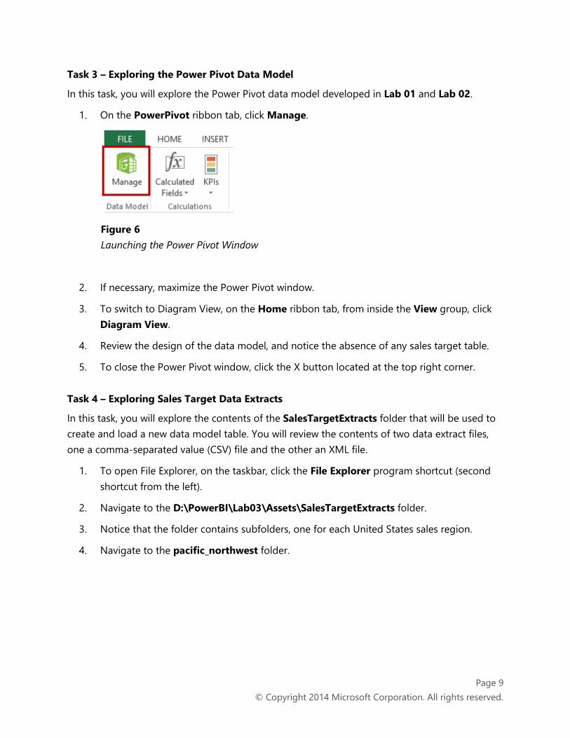
1. On the PowerPivot ribbon tab, click Manage.

Figure 6

Launching the Power Pivot Window

2. If necessary, maximize the Power Pivot window.

3. To switch to Diagram View, on the Home ribbon tab, from inside the View group, click

Diagram View.

4. Review the design of the data model, and notice the absence of any sales target table.

5. To close the Power Pivot window, click the X button located at the top right corner.

Task 4 – Exploring Sales Target Data Extracts

In this task, you will explore the contents of the SalesTargetExtracts folder that will be used to

create and load a new data model table. You will review the contents of two data extract files,

one a comma-separated value (CSV) file and the other an XML file.

1. To open File Explorer, on the taskbar, click the File Explorer program shortcut (second

shortcut from the left).

2. Navigate to the D:\PowerBI\Lab03\Assets\SalesTargetExtracts folder.

3. Notice that the folder contains subfolders, one for each United States sales region.

4. Navigate to the pacific_northwest folder.


5. Notice that the folder contains two files, the first is a CSV file that stores sales targets for

2012, and the second is an XML file that also stores sales targets but for 2013.

Note: The Pacific Northwest sales region was using a different sales planning system in

2012, and this system exported data in CSV format. Now consistent with all other

regions, the Pacific Northwest region commenced using a replacement planning

system from 2013, and it exports data in XML format.

6. To review the contents of the CSV file, right-click the

targets_pacific_northwest_2012.csv file, and then select Open.

Note: By default, a CSV file will open in Excel.

7. In Excel, notice that the data is structured with quarters across the columns, and states

down the rows.

Note: The quarters are calendar quarters, meaning that Q1 represents an aggregate

value for January, February and March.

8. Notice also that there are no target values in Q1 for Hawaii or Wyoming, and this is

represented by the dash character (-).

9. To close the CSV file, on the File ribbon tab, select Close.

10. When prompted to save changes, click Don’t Save.

11. Switch to File Explorer.

12. To review the contents of the XML file, right-click the

targets_pacific_northwest_2013.xml file, and then select Edit.

Note: By default, an XML file will open for editing in Notepad.


13. In Notepad, notice that the data is structured with a targets element that includes year

and region attributes, and nested within it are target elements with attributes of period,

state and sales.

Note: The periods represent calendar months within the specified year (i.e. 1 is January,

2 is February, etc.).

14. To close the XML file, in Notepad, on the File menu, select Exit.

15. Leave the File Explorer window open.

Task 5 – Creating a Power Query Query

In this task, you will create a Power Query query to source data from the CSV file. The query will

have the following characteristics:

Three columns: Date (type Date), StateCode (Text) and SalesTarget (Whole Number)

Monthly sales target values, calculated by dividing the quarterly sales target by 3

This query will be combined with another Power Query query that you will develop later in this

lab.

1. Switch to the Excel workbook.

2. On the Power Query ribbon tab, from inside the Get External Data group, click From

File, and then select From CSV.

Figure 7

Retrieving Data From a CSV File


3. In the Browse window, navigate to the

D:\PowerBI\Lab03\Assets\SalesTargetExtracts\pacific_northwest folder.

4. Select the targets_pacific_northwest_2012.csv file, and then click OK.

5. When the Query Editor window opens, if necessary, maximize the window.

6. In the Query Settings pane (located at the right), in the Name box, replace the text with

SalesTarget_CSV_Legacy.

Note: This query will import legacy data exported by a former planning system. There

is only one CSV file, representing planning values for calendar year 2012.

7. In the Query Settings pane, in the Applied Steps list, notice that three steps were

automatically generated to source the data content, promote the first row to column

names, and change column data types.

Figure 8

Reviewing the Query Steps

8. To visualize the query steps, select the Source step, and notice that the query result

represents the raw data sourced from the CSV file, and that the columns are generically

named.

9. If the formula bar (located below the ribbon) is not visible, on the View ribbon tab, check

Formula Bar.

Figure 9

Showing the Formula Bar


10. In the formula bar, review the expression for the selected step to source the data from a

CSV document.

Note: It is not important to understand the details of the formula.

Most Power Query step formulae are generated automatically by using commands

available on the ribbon or from context menus. It is possible to create or modify the

formula for any step directly in the formula bar.

11. Select the First Row as Header step, and notice that the query result column names are

now based on the values from the first data row.

12. Select the Changed Type step, and notice that the values in the Q2, Q3 and Q4 columns

are right-justified and italicized.

13. Notice also that the data in the Q1 column is not formatted in this way, as the data type

change was not applied due to the presence of non-numeric values for the states of

Hawaii and Wyoming.

Note: Recall that the presence of a dash character represents a zero amount.

14. In the Applied Steps list, ensure that the last step is selected.

Note: Additional steps will be inserted after the currently selected step.

15. To rename the Code column name, right-click the Code column header, and then select

Rename.

16. Replace the column name text with StateCode, and then press Enter.

17. To remove the State column, right-click the State column header, and then select

Remove.

18. To multi-select the four quarter columns, first select the Q1 column header, and then

while pressing the Shift key, select the Q4 column header.

19. To unpivot the selected columns, right-click any column header within the selection, and

then select Unpivot Columns.

20. To rename the Attribute column name, right-click the Attribute column header, and

then select Rename.


21. Replace the column name text with QuarterNumber, and then press Enter.

22. Repeat the previous two steps to rename the Value column to QuarterSalesTarget.

23. To remove the leading Q character before each quarter number, right-click the

QuarterNumber column header, and then select Replace Values.

24. In the Replace Values window, in the Value to Find box, enter Q.

Figure 10

Configuring the Replace Values Step

25. Click OK.

26. To convert the QuarterNumber and QuarterSalesTarget column data types, multi-

select the two columns, right-click any column header within the selection, and then

select Change Type | Whole Number.

27. In QuarterSalesTarget column, notice that the attempt to convert the dash characters

has resulted in errors.

28. In row 9, notice the Error link.

Figure 11

Locating the Error Link

29. To review the error details, create a new step to drill down by clicking an Error link.

30. Notice that the error was raised because the dash character could not be converted to a

number.


31. To remove the step, in the Query Settings pane, in the Applied Steps list, for the last

step, click the X icon.

Figure 12

Removing the Step

32. To remove rows that contain errors, right-click the QuarterSalesTarget column header,

and then select Remove Errors.

Note: Recall that the dash character represents a sales target value of zero. Removing

the errors effectively removes rows that represent zero sales targets.

33. To add a new column, on the Add Column ribbon tab, click Add Custom Column.

34. In the Add Custom Column window, in the New Column Name box, replace the text

with QuarterMonthNumber.

35. In the Custom Column Formula box, enter the following formula.

Power Query Formula Language

{1..3}

Note: The formula will create a list consisting of an item for each value within the

numeric range from 1 to 3. This list is required to form a Cartesian product with the

query rows in order to lower the query grain from quarter to month (i.e. each quarter

consists of three months).

36. Click OK.

37. To expand the list, and to generate a Cartesian product with the query rows, in the

QuarterMonthNumber column header, click .


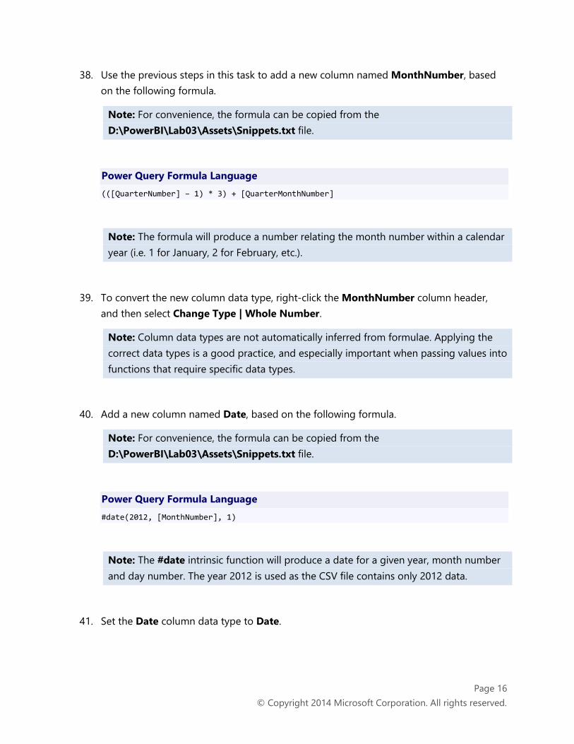
38. Use the previous steps in this task to add a new column named MonthNumber, based

on the following formula.

Note: For convenience, the formula can be copied from the

D:\PowerBI\Lab03\Assets\Snippets.txt file.


(([QuarterNumber] – 1) * 3) + [QuarterMonthNumber]

Note: The formula will produce a number relating the month number within a calendar

year (i.e. 1 for January, 2 for February, etc.).

39. To convert the new column data type, right-click the MonthNumber column header,

and then select Change Type | Whole Number.

Note: Column data types are not automatically inferred from formulae. Applying the

correct data types is a good practice, and especially important when passing values into

functions that require specific data types.

40. Add a new column named Date, based on the following formula.




#date(2012, [MonthNumber], 1)

Note: The #date intrinsic function will produce a date for a given year, month number

and day number. The year 2012 is used as the CSV file contains only 2012 data.

41. Set the Date column data type to Date.


42. To create a column of monthly sales target values, select the QuarterSalesTarget

column header, and then on the Add Column ribbon tab, from inside the From Number

group, click Standard, and then select Divide (Integer).

Figure 13

Creating a New Column Based on a Numeric Operation

Note: The Divide (Integer) option will produce an integer result, and without rounding

(e.g. 9/10 will produce a result of 0). Interestingly, the data type applied to a column

created in this way will be Decimal Number.

43. In the Integer-Divide window, in the Value box, enter 3, and then click OK.

44. Rename the new column to SalesTarget, and then set the column data type to Whole

Number.

45. To remove non-required columns, while pressing the Control key, multi-select the

StateCode, Date and SalesTarget columns.

46. Right-click any column header in the selection, and then select Remove Other Columns.

47. To reorder the Date column, right-click the Date column header, and then select Move |

Left.

Note: It is also possible to reorder columns by dragging and dropping column headers.


48. Ensure that the final query result looks like the following.

Figure 14

Reviewing the Final Query Result

49. To close the query without loading the result to an Excel table, on the Home ribbon tab,

from inside the Query group, click the Close & Load dropdown arrow, and then select

Close & Load To.

Figure 15

Locating the Close & Load To Command


50. In the Load To window, select the Only Create Connection option.

Figure 16

Reviewing the Load Settings

51. Click Load.

Note: This configuration will not load the data, and will simply save the query definition

within the workbook. The query result will be combined with another query that you

will create later in this lab.

52. In Excel, in the Workbook Queries pane, notice the list of workbook queries.

Note: The StatePopulation query was created in Lab 02.

53. Hover over the SalesTarget_CSV_Legacy query to show the peek at the data preview.


Task 6 – Creating a Power Query Function

In this task, you will create a Power Query function to source data from a single XML file, which

represents data exported from the current planning system. The function will have the following

characteristics:

Three columns: Date (type Date), StateCode (Text) and SalesTarget (Whole Number)

Allow sourcing data from any identically structured XML file

This function will be invoked in a Power Query query created in the next task.


File, and then select From XML.

Figure 17

Retrieving Data From an XML File

2. In the Browse window, navigate to the

D:\PowerBI\Lab03\Assets\SalesTargetExtracts\pacific_northwest folder.

3. Select the targets_pacific_northwest_2013.xml file, and then click OK.


5. In the Query Settings pane, in the Name box, replace the text with SalesTarget_XML.

6. Notice that the query result consists of a single row, which is the target element from

the XML document.

Note: The elements nested within the targets attribute are available as a table, and the

attribute values of the targets element are available as columns.


7. Notice that the value in the Attribute:year column is right-justified and italicized, as the

second query step set the column data type to Whole Number.

8. Rename the Attribute:year column to Year.

9. Remove the Attribute:region column.

10. To expand the target table (which represents inner XML elements), in the target column

header, click , and then to expand all columns (the element attributes), click OK.

11. Rename, and set the data types, for the following columns.

Tip: If you rename all column names first, and then set the column data types second,

each similar action will be consolidated into a single query step.

Column Name New Column Name Data Type

target.Attribute:period MonthNumber Whole Number

target.Attribute:state StateCode Text (was set by default)

target.Attribute:sales SalesTarget Whole Number

12. Add a new column named Date, based on the following formula.




#date([Year], [MonthNumber], 1)

13. Multi-select the StateCode, SalesTarget and Date columns, and then remove all other

columns.

14. Resequence the columns in this order: Date, StateCode and SalesTarget.

15. To remove rows with zero sales target values, in the SalesTarget column header, click

, and then select Number Filters | Does Not Equal.


16. In the Filter Rows window, in the top right box, enter 0.

Figure 18

Configuring the Filter Value Step

17. Click OK.

18. To convert the query to a function, on the View ribbon tab, click Advanced Editor.

Figure 19

Locating the Advanced Editor

19. In the Advanced Editor window, notice that they query is in fact a sequence of steps,

with each step defined by a formula.

Note: Each step, except the first, is identified by a unique name preceded by the #

symbol. This name is in fact a variable, and you will notice the use of the variable in the

step that follows. Each step is a transformation of the preceding step.


20. Carefully insert the following parameter declaration at the very top of the script.

Figure 20

Inserting the Parameter Declaration

Note: Functions are written by listing the function’s parameters in parentheses,

followed by the “goes-to” symbol (=>), followed by the expression defining the

function.

21. To insert the parameter into the script body, in the Source line, replace the full file path,

including the double-quote symbols, with FilePath.

22. Verify that the Source line reads as follows.

Figure 21

Inserting the Parameter Into the Script Body

23. Click Done.

24. In the Query Editor window, notice that the Invoke | Function contextual ribbon tab is

displayed, with a single command to allow the invocation of the function.

Note: The function will be invoked by a new Power Query query in the next task.

25. In the Query Settings pane, notice also that the query is now reduced to a single step.

26. To close the function, on the Home ribbon tab, from inside the Query group, click the

Close & Load dropdown arrow, and then select Close & Load.


27. In Excel, in the Workbook Queries pane, notice that the SalesTarget_XML function is

decorated with a different icon.

Figure 22

Locating the Function Icon

Note: As you will see in the next task, functions allow the reuse of logic and data within

the workbook.

Task 7 – Invoking the Power Query Function and Combining Queries

In this task, you will create a final Power Query query to generate sales target data for all XML

data files, and then combine the result with the SalesTarget_CSV_Legacy query.

1. On the Power Query ribbon tab, from inside the Workbook Settings group, click Fast

Combine.

Note: Enabling Fast Combine allows Power Query to relate two different data sources

together within a single query. This may have the effect of improving performance, but

could also breach privacy by exposing data from one data source to the other. By

default this behavior is not enabled. In this lab, however, it will be enabled as there is

no violation of privacy when working with the data extract files.

2. When prompted to enable Fast Combine, click Enable.



File, and then select From Folder.

Figure 23

Retrieving Data From a Folder

4. In the Folder window, click Browse.

5. In the Browse For Folder window, expand Computer, and then expand the folder

hierarchy to select the D:\PowerBI\Lab03\Assets\SalesTargetExtracts folder, and then

click OK.

6. In the Folder window, click OK.


8. In the Query Settings pane, in the Name box, replace the text with SalesTarget.

9. Notice that the query result consists of a row for each file found within the folder,

including files found in sub-folders.

10. To remove rows representing non-XML files, in the Extension column header, click ,

uncheck .csv, and then click OK.

11. To add a new column containing the full file path, first select the Folder Path column

(you may need to horizontally scroll to the right), and then while pressing the Control

key, select the Name column.

12. On the Add Column ribbon tab, from inside the From Text group, click Merge

Columns.


13. In the Merge Columns window, click OK.

Note: A separator character is not required. The values of the new column are

produced by concatenating the selected columns in the order in which they are

selected.

14. Rename the new column (located last) to FilePath.

15. Remove all columns except the FilePath column.

16. Add a new column named SalesTarget, based on the following formula.




SalesTarget_XML([FilePath])

Note: This formula invokes the SalesTarget_XML function which was created in the

previous task.

17. To expand the entire table for each row, in the SalesTarget column header, click , and

then to expand all columns, click OK.

18. Rename each of the three new columns to Date, StateCode and SalesTarget.

Tip: An alternate – and possibly quicker – way to rename the columns is to carefully

edit the formula of the Expand SalesTarget query step. You will notice that the new

column names are listed toward the end of the formula.

19. Remove the FilePath column.

20. To combine the query with the CSV data, on the Home ribbon tab, from within the

Combine group, click Append Queries.

21. In the Append window, in the dropdown list, select the SalesTarget_CSV_Legacy query.

22. Click OK.


23. Set the following data types for each of the following columns.

Column Name Data Type

Date Date

StateCode Text

SalesTarget Whole Number

24. To close the query and load the workbook data model, on the Home ribbon tab, from

inside the Query group, click the Close & Load dropdown arrow, and then select

Close & Load To.

Figure 24

Locating the Close & Load To Command


25. In the Load To window, select the Only Create Connection option, and then check the

Add this Data to the Data Model checkbox.

Figure 25

Reviewing the Load Settings

26. Click Load.

27. In Excel, in the Workbook Queries pane, notice the addition of the SalesTarget query,

and that 1,179 rows were loaded.

28. Hover over the SalesTarget query to show the peek at the data preview.

29. Review the preview data and notice the last refresh time, load settings and data sources.

Task 8 – Organizing the Workbook Queries

In this task, you will organize the workbook queries into logical groups.

1. In the Workbook Queries pane, while pressing the Control key, multi-select the

following two queries: SalesTarget_CSV_Legacy, and SalesTarget_XML.

2. Right-click the selection and then select Move to Group | Create Group.

3. In the Create Group window, in the Name box, enter Preparation, and then click OK.


4. In the Workbook Queries pane, notice that the queries are now organized into groups.

5. Repeat the previous steps in this task to move the remaining two queries (in the default

Other Queries group) into a new group named Data Model.


Exercise 2: Integrating the Solution with the

Workbook Data Model

In this exercise, you will refresh the Power Query data, and integrate the resulting table to

produce sales target calculations and a KPI. Finally, you will create a PivotTable report to

monitoring sales performance.

Task 1 – Exploring the Power Pivot Data Model

In this task, you will open the Power Pivot window to review the data loaded into the workbook

data model, and refresh the data to load in 2014 sales targets.

1. On the PowerPivot ribbon tab, click Manage.

2. In the PowerPivot window, to switch to Diagram View, on the Home ribbon tab, from

inside the View group, click Diagram View.

3. Notice the addition of the SalesTarget table (you may need to scroll to the far right of

the diagram).

4. To review the data, right-click the SalesTarget table, and then select Go To.

5. In the record navigator (located at the bottom left of the window), notice the record

count of 1,179.

6. Switch to File Explorer (opened in Task 4).

7. Navigate to the D:\PowerBI\Lab03\Assets folder.

8. To extract the 2014 data extract files, right-click the SalesTarget_2014.zip file, and then

select Extract All.

9. In the Extract Compressed (Zipped) Folders window, click Browse.

10. In the Select a Destination window, expand Computer, and then expand the folder

hierarchy to select the D:\PowerBI\Lab03\Assets\SalesTargetExtracts folder, and then

click OK.

11. If required, uncheck the Show Extracted Files When Complete checkbox.

12. Click Extract.

13. In File Explorer, navigate to the SalesTargetExtracts folder, and then to the

pacific_northwest folder, and notice the addition of the 2014 data extract file.


14. Switch to the Power Pivot window.

15. To refresh the SalesTarget table, on the Home ribbon tab, click the arrow beneath the

Refresh command, and then select Refresh.

Figure 26

Selecting Refresh

16. In the Data Refresh window, when processing is complete, notice that 1,785 rows were

loaded.

Note: The Power Query extracted data from all XML files, including the recently added

2014 data extracts.

17. Click Close.

Task 2 – Developing the Data Model Enhancements

In this task, you will integrate the SalesTarget table into the workbook data model, and then

define sales target calculations and a KPI.

1. To switch to Diagram View, on the Home ribbon tab, from inside the View group, click

Diagram View.

2. To move the SalesTarget table, drag the table header to position the table nearer to the

Date and State tables.


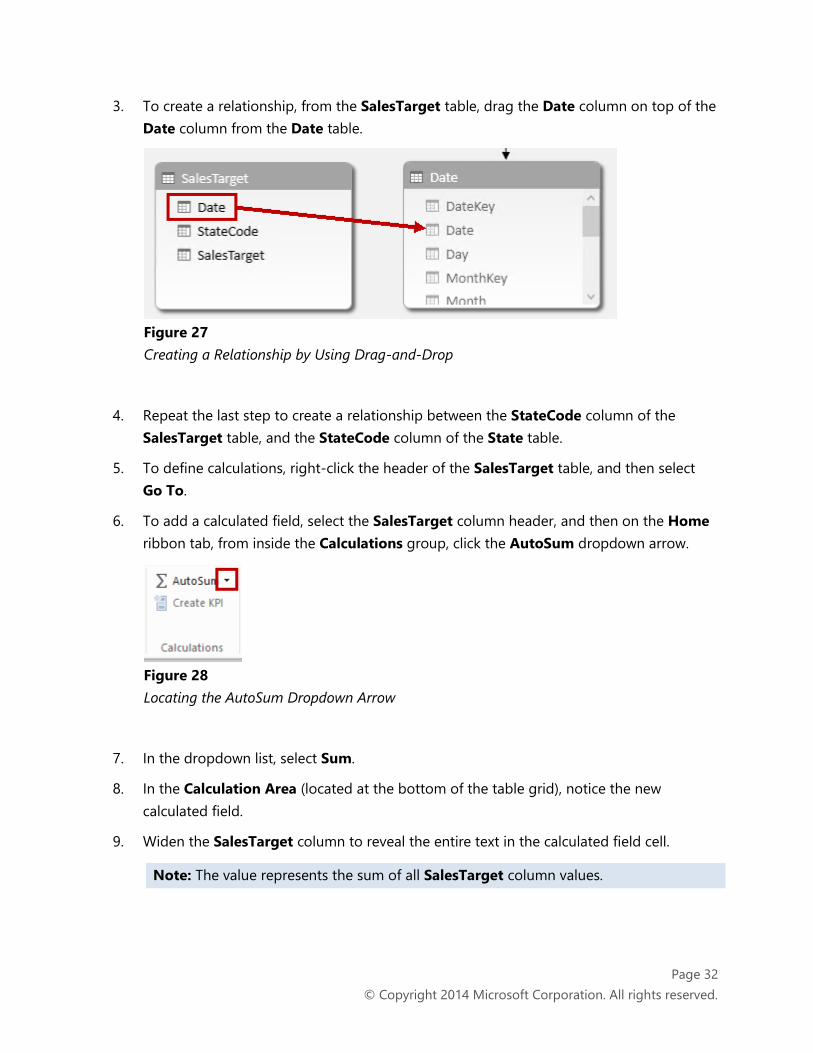
3. To create a relationship, from the SalesTarget table, drag the Date column on top of the

Date column from the Date table.

Figure 27

Creating a Relationship by Using Drag-and-Drop

4. Repeat the last step to create a relationship between the StateCode column of the

SalesTarget table, and the StateCode column of the State table.

5. To define calculations, right-click the header of the SalesTarget table, and then select

Go To.

6. To add a calculated field, select the SalesTarget column header, and then on the Home

ribbon tab, from inside the Calculations group, click the AutoSum dropdown arrow.

Figure 28

Locating the AutoSum Dropdown Arrow

7. In the dropdown list, select Sum.

8. In the Calculation Area (located at the bottom of the table grid), notice the new

calculated field.

9. Widen the SalesTarget column to reveal the entire text in the calculated field cell.

Note: The value represents the sum of all SalesTarget column values.


10. In the formula bar (located above the table grid), notice the DAX expression that was

generated.

11. To rename the calculated field to Sales Target, in the formula bar, modify the first

portion of the expression as follows.

DAX

Sales Target:=SUM([SalesTarget])

12. Press Enter.

13. To format the calculated field, in the Calculation Area, right-click the calculated field,

and then select Format.

14. In the Formatting window, in the Category list, select Currency.

Figure 29

Reviewing the Sales Target Calculated Field Formatting

15. Click OK.

16. To create a second calculated field, select the cell immediately beneath the Sales Target

calculated field.


17. In the formula bar, enter the following expression.

Note: For convenience, the expression can be copied from the


DAX

Variance:=[Sales] - [Sales Target]

18. Press Enter.

19. Repeat the steps in this task to format the new calculated field as Currency.

Note: The low negative variance is due to the fact that the data model does not yet

include actual sales data for the year 2014.

20. Immediately beneath the Variance calculated field, create a third calculated field by

using the following expression.



DAX

Variance%:=DIVIDE([Variance], [Sales Target])

Note: The DIVIDE function divides two expressions, providing that the second

expression results in a non-zero number. If the second argument results in zero or

blank (missing), then the function will return blank.

If the calculated field returns zero it means sales exactly achieved target. Otherwise, a

positive value means sales exceeded target, while a negative value means sales did not

achieve target.

21. To format the Variance% calculated field, in the Calculation Area, right-click the

calculated field, and then select Format.


22. In the Formatting window, in the Category list, select Number, and then in the Format

dropdown list, select Percentage.

Figure 30

Reviewing the Calculated Field Formatting

23. Click OK.

24. Immediately beneath the Variance% calculated field, create a fourth calculated field by

using the following expression.



DAX

Sales Performance:=[Variance%]

25. Format the calculated field as percentage.

26. To create a KPI, right-click the Sales Performance calculated field, and then select

Create KPI.

27. In the Key Performance Indicator (KPI) window, in the Define Target Value section,

select the Absolute Value option.

28. In the corresponding box, replace the value with 1.

Note: The thresholds of this KPI will be measured solely by the value of the Variance%

calculated field. The absolute value will play no role, but is configured to meet the

requirement to define a target value.


29. In the Define Status Thresholds boxes, modify the first value to -0.1, and the second

value to 0, and then press Enter.

Note: As the values are so near each other the user interface almost overlays them.

The value of -0.1 is -10%.

30. Verify the KPI configuration looks like the following.

Figure 31

Reviewing the KPI Configuration

31. In the Select Icon Style section, select the sixth style from the left.

Figure 32

Reviewing the KPI Icon Style

32. Click OK.


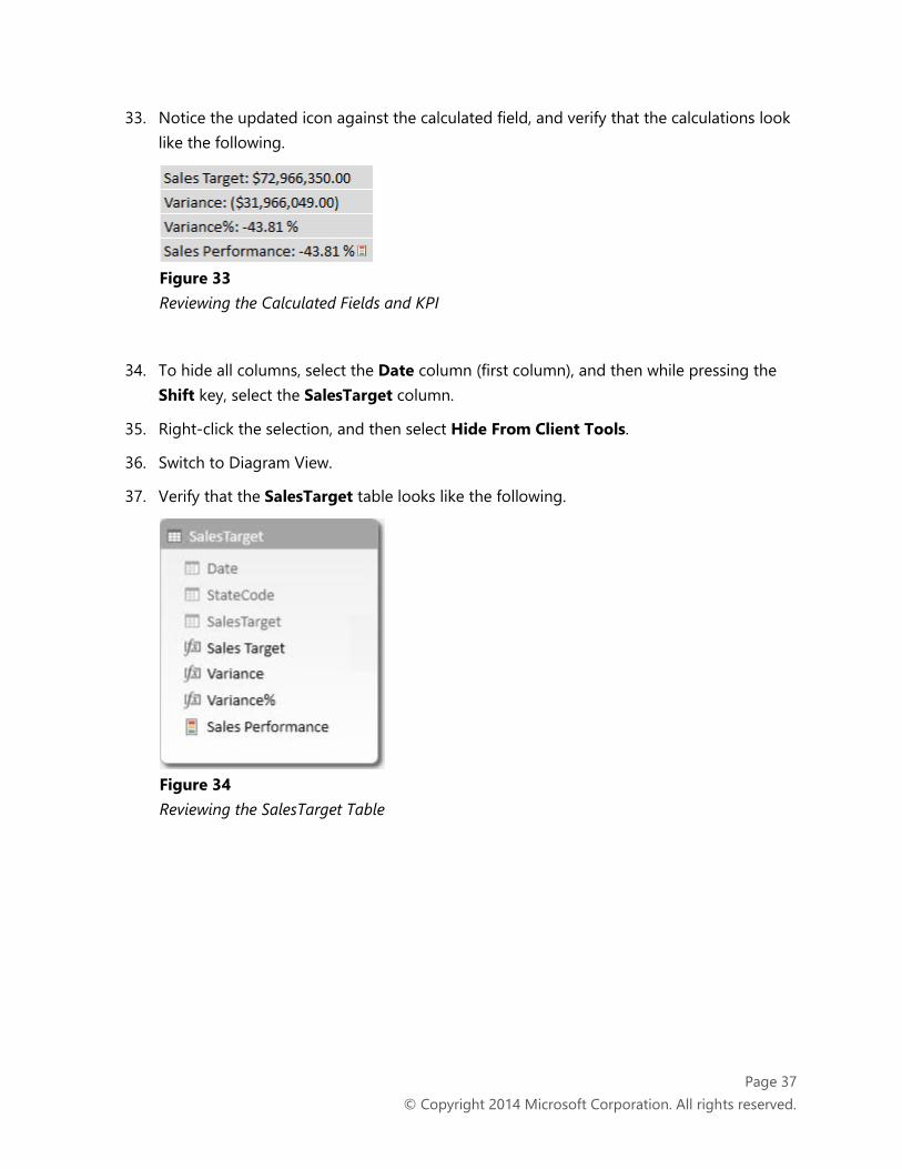
33. Notice the updated icon against the calculated field, and verify that the calculations look

like the following.

Figure 33

Reviewing the Calculated Fields and KPI

34. To hide all columns, select the Date column (first column), and then while pressing the

Shift key, select the SalesTarget column.

35. Right-click the selection, and then select Hide From Client Tools.

36. Switch to Diagram View.

37. Verify that the SalesTarget table looks like the following.

Figure 34

Reviewing the SalesTarget Table


Task 3 – Creating a PivotTable Report

In this task, you will create a PivotTable report to monitor sales performance.

1. On the Home ribbon tab, click the arrow beneath PivotTable, and then select

PivotTable.

Figure 35

Adding a Single PivotTable

2. In the Create PivotTable window, to create a new worksheet, click OK.

3. Notice that a PivotTable has been added to an Excel worksheet, and that the PivotTable

Fields pane is open (located at the right).

4. To close the Workbook Queries pane, on the Power Query ribbon tab, from inside the

Manage group, click Workbook Queries.

5. To rename the worksheet, right-click the Sheet1 worksheet tab, and then select Rename.

6. Rename the worksheet to Sales Performance Monitoring, and then press Enter.

7. Expand all five groups in the PivotTable Fields pane, and notice the resources that are

available to produce the PivotTable layout.


8. To add a report filter, in the Date table, drag the Calendar hierarchy into the Filters drop

zone.

Figure 36

Adding the Calendar Hierarchy to the PivotTable Filters

9. In the PivotTable report filter (cell C1), click the down arrow, expand the All member,

select CY2013 | CY2013 Q3 | 2013-Sep, and then click OK.

10. In the PivotTable Fields pane, in the Sales group, check the Sales field.

11. In the SalesTarget group, check the Sales Target, Variance and Variance% fields.

12. Expand the Sales Performance KPI, and then check the Status field.

13. To introduce row labels, in the State group, check the States hierarchy.

14. In the PivotTable, expand the Pacific Northwest member (cell B7) to reveal the states.

15. To sort the states in ascending order of variance, right-click any cell in the Variance%

value, and then select Sort | Sort Smallest to Largest.


16. Verify that the PivotTable report looks like the following.

Figure 37

Reviewing the PivotTable Report

17. Notice that variance amount less than 10% have a red status indicator, and others that

are less than 0% are yellow.

Task 4 – Finishing Up

In this task, you will finish up by closing Excel.

1. To save the workbook, on the File ribbon tab, click Save.

2. To close Excel, click the X button in the top right corner.

3. Close the File Explorer window.

Summary

In this lab, you used Power Query to extend the Power Pivot workbook created in Lab 02 with

additional data to enable the performance monitoring of sales against sales target. The sales

target data by state was sourced from CSV and XML data extract files, and three Power Query

queries were developed to effectively extract, transform and load the data into the workbook

data model.

Developing a Power Query Solution in Excel...

Documents

Transcript of Developing a Power Query Solution in Excel...