P021-1

Developing a 3D coupled hydrodynamic and ecological model to be used in coastal management

Olof LIUNGMAN1, Patricia MORENO-ARANCIBIA2

1 DHI Sweden, Kyrkogatan 3, 222 22 Lund, Sweden, e-mail: olof.liungman@dhi.se 2 DHI Sweden, Svartmangatan 18, 111 29 Stockholm, Sweden, e-mail: patricia.moreno-arancibia@dhi.se

Keywords Hydrodynamic, biochemical, modelling, MIKE3, MIKE ECO Lab, nitrogen, phosphorous, Himmerfjärden estuary, coastal management.

Abstract

Himmerfjärden is an estuary located on the east coast of Sweden. In the inner part of Himmerfjärden a sewage treatment plant discharges treated sewage. The Himmerfjärden estuary is a well-researched area and has been the subject of a long-term monitoring program. Currently, a large-scale experiment is underway to determine the effect of 1) decreasing the degree of nitrogen treatment of the discharge and 2) moving the location of the discharge closer to the surface. The goal is to develop a coastal management strategy that limits the blooms of nitrogen-fixing cyanobacteria in Himmerfjärden, while maintaining water quality and avoiding eutrophication.

DHI Sweden has, in collaboration with Stockholm University, started to develop a 3-dimensional coupled hydrodynamic and biochemical model that can be used to describe the circulation and the nutrient/plankton dynamics in the Himmerfjärden estuary. Once this model has been calibrated and validated it can be used to obtain a deeper understanding of the large-scale experiments or for scenario simulations.

This presentation focuses on the methodology and tools employed in developing the coupled hydrodynamic and biochemical models. The hydrodynamic model is based on MIKE3 while the biochemical model is developed using MIKE ECO Lab. The results of the hydrodynamic modelling in Himmerfjärden, including a comparison with temperature and salinity measurements, will be discussed. Preliminary results of the biochemical modelling will also be presented. The presentation will conclude with a discussion about further development of the biochemical model.

INTRODUCTION

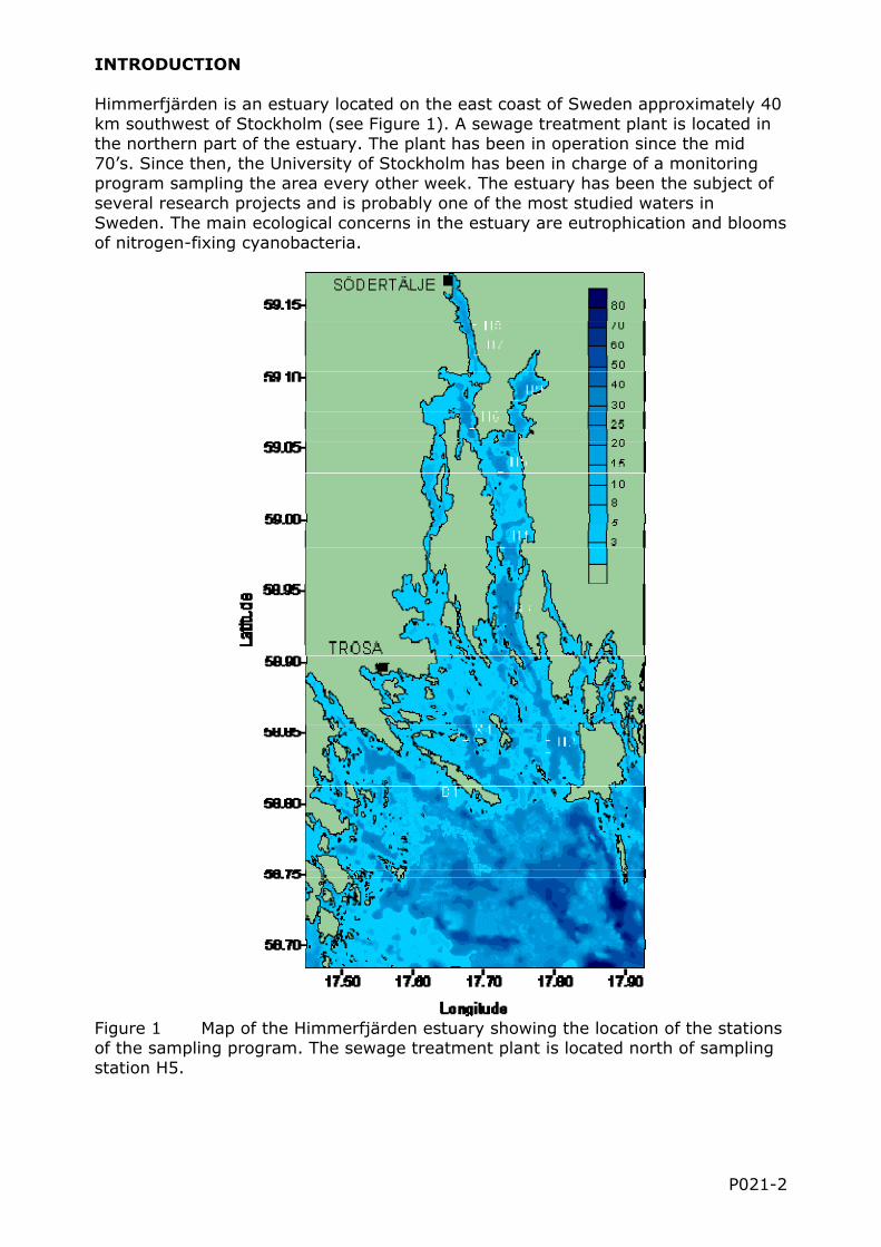
Himmerfjärden is an estuary located on the east coast of Sweden approximately 40 km southwest of Stockholm (see Figure 1). A sewage treatment plant is located in the northern part of the estuary. The plant has been in operation since the mid 70’s. Since then, the University of Stockholm has been in charge of a monitoring program sampling the area every other week. The estuary has been the subject of several research projects and is probably one of the most studied waters in Sweden. The main ecological concerns in the estuary are eutrophication and blooms of nitrogen-fixing cyanobacteria.

Figure 1 Map of the Himmerfjärden estuary showing the location of the stations of the sampling program. The sewage treatment plant is located north of sampling station H5.

P021-2

At the moment, a large-scale experiment is being conducted in the Himmerfjärden estuary to study the effect of changing the nitrogen discharge from the sewage treatment plant. The key question is whether it is possible to reduce the blooms of nitrogen-fixing cyanobacteria by increasing the amount of dissolved inorganic nitrogen in the water while avoiding degrading the environmental status regarding eutrophication. The experiment is carried out in two phases

1. During 2007-2008 the sewage water is not treated with regard to nitrogen.More nitrogen will therefore be released into the Himmerfjärden estuary. Thehope is that the amount of dissolved inorganic nitrogen in the water issufficiently large that all the phosphorous is taken up during the springbloom. If phosphorous is depleted, the cyanobacteria cannot fixate nitrogen(N2), reducing the risk of cyanobacteria blooms during the summer.

2. During 2009-2010 the discharge is moved closer to the surface and nitrogentreatment is re-introduced. The original discharge was located at 25 m depth,which is close to the bottom. By moving the discharge to a depth to 10 mmore nitrogen will be available where it can be taken up by thephytoplankton.

In connection with these large-scale experiments DHI Sweden has performed coupled hydrodynamic-ecological modelling of Himmerfjärden. The goal is to develop a model that can be used to study the effect of changing the nutrient discharge from the sewage treatment plant on the ecological conditions in the estuary.

BACKGROUND

The Himmerfjärden estuary is located in the southern part of the Stockholm archipelago. It has a surface area of about 174 km2 and a mean depth of 17 m. The estuary is made up a number of basins connected by narrow and shallow sills (see Figure 2).

Figure 2 North to south transect of Himmerfjärden. The location of the sampling stations is marked. Compare with map in Figure 1.

The hydrodynamic conditions are described in terms of the circulation (currents), temperature, salinity and sea level. The vertical distribution of temperature and salinity gives an indication of how stratified or well-mixed the water column is, which is of great importance for the ecological processes in the water.

In an estuary the hydrodynamic conditions are affected by a number of processes. In the Himmerfjärden estuary, it is mostly the local wind, fresh water discharges from Lake Mälaren and surrounding drainage basins and the stratification in the adjacent coastal areas that affect the circulation and stratification/mixing in the estuary. Sea level changes outside the estuary have a minor effect as there are no

P021-3

P021-4

tides in the Baltic Sea. The narrow and shallow sills between the different sub-basins play an important role as they hinder the exchange of the deep water.

In Himmerfjärden the nutrients, phytoplankton and zooplankton follow a typical annual cycle. During the winter, the concentration of nutrients is high while the concentration of phytoplankton and zooplankton are low. The water column is well-mixed and the nutrients are homogenously distributed. As spring approaches and the light levels increase, the phytoplankton biomass increases as the phytoplankton start taking up the nutrients dissolved in the water. During the spring bloom, the phytoplankton biomass is the largest. The zooplankton biomass remains fairly low as the water is still too cold for any significant grazing to take place. At the end of the spring bloom, the nutrients have been depleted. At the beginning of the summer, the water starts warming up creating a stratified water column. This makes it difficult for the nutrients in the deeper water to be mixed up towards the surface. During the spring and summer, phytoplanktons die and become detritus. Both phytoplankton and detritus sink towards the bottom where a fraction of the biomass settles and the rest is returned to the water column as inorganic nutrients. At the end of the summer when the water is the warmest, zooplankton grazing increases and zooplankton biomass reaches its peak. During the fall, the stratification breaks up and the water becomes mixed and nutrients are mixed from the bottom toward the surface. If the light levels are sufficiently high when the water becomes mixed it is possible to have a fall bloom. The amount of inorganic nutrients builds up during the winter when organic material decays and nutrient uptake is small.

The distribution of nutrients and phytoplankton are not only influenced by ecological processes but also by the hydrodynamic conditions. The currents redistribute the nutrients and phytoplankton and thereby determine if the phytoplankton are in a region with sufficient nutrients and light for primary production. Stratification prevents the mixing of nutrient and may limit the access to nutrient in the euphotic zone where light is available. In addition, many biological processes, e.g. zooplankton grazing, are temperature dependent and increase with increasing temperature. In the Himmerfjärden estuary, the inflow of oxygen-rich water from the Baltic Sea plays an important role as it affects the oxygen conditions at the bottom and thereby the release of phosphorous from the sediments.

METHODOLOGY

To be able to describe and quantify the ecological processes in the Himmerfjärden a numerical model is set up. The model consists of two parts: a hydrodynamic model, which calculates the currents, temperature, salinity and sea water level and an ecological part, which calculates the nutrient dynamics, primary production and other biological processes. The ecological model is coupled and forced by the hydrodynamic one.

Both the hydrodynamic and ecological models are implemented using tools included in the modelling suite MIKE by DHI. This is commercial software used by a large number of users around the world to answer questions related to environmental water problems.

P021-5

Hydrodynamic model

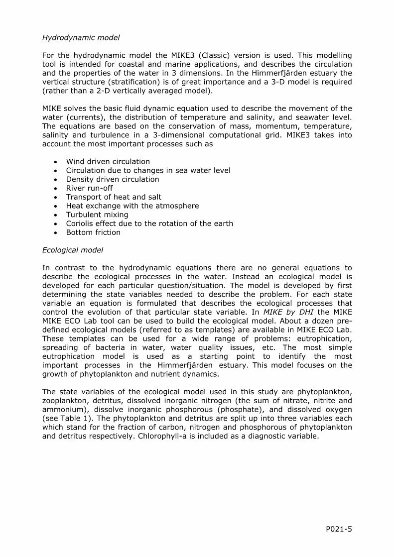
For the hydrodynamic model the MIKE3 (Classic) version is used. This modelling tool is intended for coastal and marine applications, and describes the circulation and the properties of the water in 3 dimensions. In the Himmerfjärden estuary the vertical structure (stratification) is of great importance and a 3-D model is required (rather than a 2-D vertically averaged model).

MIKE solves the basic fluid dynamic equation used to describe the movement of the water (currents), the distribution of temperature and salinity, and seawater level. The equations are based on the conservation of mass, momentum, temperature, salinity and turbulence in a 3-dimensional computational grid. MIKE3 takes into account the most important processes such as

• Wind driven circulation• Circulation due to changes in sea water level• Density driven circulation• River run-off• Transport of heat and salt• Heat exchange with the atmosphere• Turbulent mixing• Coriolis effect due to the rotation of the earth• Bottom friction

Ecological model

In contrast to the hydrodynamic equations there are no general equations to describe the ecological processes in the water. Instead an ecological model is developed for each particular question/situation. The model is developed by first determining the state variables needed to describe the problem. For each state variable an equation is formulated that describes the ecological processes that control the evolution of that particular state variable. In MIKE by DHI the MIKE MIKE ECO Lab tool can be used to build the ecological model. About a dozen pre-defined ecological models (referred to as templates) are available in MIKE ECO Lab. These templates can be used for a wide range of problems: eutrophication, spreading of bacteria in water, water quality issues, etc. The most simple eutrophication model is used as a starting point to identify the most important processes in the Himmerfjärden estuary. This model focuses on the growth of phytoplankton and nutrient dynamics.

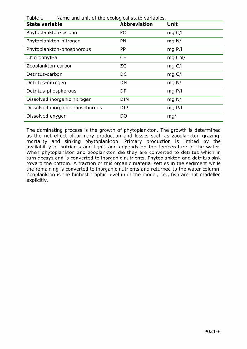
The state variables of the ecological model used in this study are phytoplankton, zooplankton, detritus, dissolved inorganic nitrogen (the sum of nitrate, nitrite and ammonium), dissolve inorganic phosphorous (phosphate), and dissolved oxygen (see Table 1). The phytoplankton and detritus are split up into three variables each which stand for the fraction of carbon, nitrogen and phosphorous of phytoplankton and detritus respectively. Chlorophyll-a is included as a diagnostic variable.

P021-6

Table 1 Name and unit of the ecological state variables. State variable Abbreviation Unit

Phytoplankton-carbon PC mg C/l

Phytoplankton-nitrogen PN mg N/l

Phytoplankton-phosphorous PP mg P/l

Chlorophyll-a CH mg Chl/l

Zooplankton-carbon ZC mg C/l

Detritus-carbon DC mg C/l

Detritus-nitrogen DN mg N/l

Detritus-phosphorous DP mg P/l

Dissolved inorganic nitrogen DIN mg N/l

Dissolved inorganic phosphorous DIP mg P/l

Dissolved oxygen DO mg/l

The dominating process is the growth of phytoplankton. The growth is determined as the net effect of primary production and losses such as zooplankton grazing, mortality and sinking phytoplankton. Primary production is limited by the availability of nutrients and light, and depends on the temperature of the water. When phytoplankton and zooplankton die they are converted to detritus which in turn decays and is converted to inorganic nutrients. Phytoplankton and detritus sink toward the bottom. A fraction of this organic material settles in the sediment while the remaining is converted to inorganic nutrients and returned to the water column. Zooplankton is the highest trophic level in in the model, i.e., fish are not modelled explicitly.

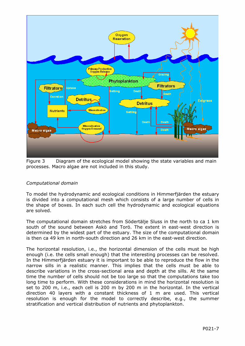
Figure 3 Diagram of the ecological model showing the state variables and main processes. Macro algae are not included in this study.

Computational domain

To model the hydrodynamic and ecological conditions in Himmerfjärden the estuary is divided into a computational mesh which consists of a large number of cells in the shape of boxes. In each such cell the hydrodynamic and ecological equations are solved.

The computational domain stretches from Södertälje Sluss in the north to ca 1 km south of the sound between Askö and Torö. The extent in east-west direction is determined by the widest part of the estuary. The size of the computational domain is then ca 49 km in north-south direction and 26 km in the east-west direction.

The horizontal resolution, i.e., the horizontal dimension of the cells must be high enough (i.e. the cells small enough) that the interesting processes can be resolved. In the Himmerfjärden estuary it is important to be able to reproduce the flow in the narrow sills in a realistic manner. This implies that the cells must be able to describe variations in the cross-sectional area and depth at the sills. At the same time the number of cells should not be too large so that the computations take too long time to perform. With these considerations in mind the horizontal resolution is set to 200 m, i.e., each cell is 200 m by 200 m in the horizontal. In the vertical direction 40 layers with a constant thickness of 1 m are used. This vertical resolution is enough for the model to correctly describe, e.g., the summer stratification and vertical distribution of nutrients and phytoplankton.

P021-7

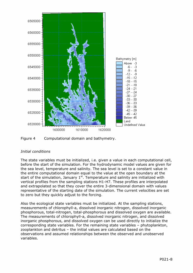
Figure 4 Computational domain and bathymetry.

Initial conditions

The state variables must be initialized, i.e. given a value in each computational cell, before the start of the simulation. For the hydrodynamic model values are given for the sea level, temperature and salinity. The sea level is set to a constant value in the entire computational domain equal to the value at the open boundary at the start of the simulation, January 1st. Temperature and salinity are initialized with vertical profiles from the sampling stations H1-H7. These profiles are interpolated and extrapolated so that they cover the entire 3-dimensional domain with values representative of the starting date of the simulation. The current velocities are set to zero but they quickly adjust to the forcing.

Also the ecological state variables must be initialized. At the sampling stations, measurements of chlorophyll-a, dissolved inorganic nitrogen, dissolved inorganic phosphorous, total-nitrogen, total-phosphorous and dissolved oxygen are available. The measurements of chlorophyll-a, dissolved inorganic nitrogen, and dissolved inorganic phosphorous, and dissolved oxygen can be used directly to initialize the corresponding state variables. For the remaining state variables – phytoplankton, zooplankton and detritus – the initial values are calculated based on the observations and assumed relationships between the observed and unobserved variables.

P021-8

P021-9

The phytoplankton-carbon is calculated based on the chlorophyll-a observations and assuming a constant carbon to chlorophyll ratio (30 g C/g Chl). The fractions of phytoplankton-nitrogen and phytoplankton-phosphorous are calculated using the Redfield ratio. The zooplankton concentration is assumed to be proportional to the phytoplankton concentration with a proportionality factor of 0.1. Detritus-phosphorous is calculated from observations of total-phosphorous which is assumed to be the sum of dissolved inorganic phosphorous, phytoplankton-phosphorous and detritus-phosphorous (zooplankton-phosphorous is neglected). Detritus-nitrogen is calculated in a similar manner except that a fraction of the total-nitrogen (0.17 mg N/l) is assumed to be biological unavailable. This fraction is subtracted from total-nitrogen before detritus-nitrogen is calculated. The conversions are summarized in Table 2.

Table 2 Summary of the conversions used to convert observations to model state variables. The same method is used for the initial fields as for the boundary conditions. 0.17 mg/l in the detritus-nitrogen equation stands for the fraction of nitrogen that is not biological available. Observations have been obtained from the University of Stockholm. Model state variable Observation Conversion

Phytoplankton-carbon - (30 mg C/mg Chl) x CH

Phytoplankton-nitrogen

- PC / 6

Phytoplankton-phosphorous

- PC / 42

Chlorophyll-a CH -

Zooplankton-carbon - 0,1 x PC

Detritus-carbon - 5 x DN

Detritus-nitrogen - TotN – DIN – 0,17 mg N/l – PN

Detritus-phosphorous - TotP – DIP - PP

Dissolved inorganic nitrogen

NH4+NO2+NO3 -

Dissolved inorganic phosphorous

PO4 -

Dissolved oxygen DO -

Model forcing

To force the coupled hydrodynamic-ecological model the following data are needed

• meteorological conditions• discharge of fresh water• conditions at the open boundary towards the Baltic Sea

P021-10

Meteorological data

To determine the meteorological forcing information of the wind conditions, precipitation and heat exchange between the sea and atmosphere are required.

The ecological model also requires solar irradiance to calculate primary production. In addition, atmospheric deposition of nitrogen is an important source. Deposition of phosphorous is assumed to be very small and therefore neglected in this model.

Fresh water and nutrient transport

The hydrodynamic and ecological models are also forced by the fresh water discharge and associated nutrient transport to the Himmerfjärden estuary. The main sources of fresh water to Himmerfjärden are

• Runoff from surrounding drainage basin in the form of monthly averages.• Discharge from Lake Mälaren. This water flows through the Södertälje sluss

where daily values of the discharge are available.• Discharge of treated water from the sewage treatment plant.

The transport of nitrogen and phosphorous to the estuary plays an important role in determining the nutrient and plankton dynamics in the estuary. Nutrients are added to the estuary through transport from land and from the sewage treatment plant. Observations of DIN, DIP, total-nitrogen and total-phosphorous are available. Phytoplankton and zooplankton from the rivers are assumed to be fresh water species that do not survive in the salty water of Himmerfjärden. They are converted to detritus. The amount of detritus-nitrogen and detritus-phosphorous is determined from the observations.

Boundary condition

Open boundaries are those where the model domain borders a water body. At such boundaries, values of the state variables must be given throughout the simulation period. In Himmerfjärden the open boundary is the one towards the Baltic Sea.

For the hydrodynamic model, sea level, temperature and salinity must be given at the open boundary. Sea level data is obtained from the automatic station located off-shore at Landsort (provided by SMHI). Temperature and salinity data from the sampling station B1, which is located just south of the open boundary, are used as boundary condition.

For the ecological model values must be given for all the ecological state variables. At the sampling station, observations are available for chlorophyll-a, dissolved inorganic nitrogen, dissolved inorganic phosphorous, total-nitrogen, total-phosphorous, and dissolved oxygen. These observations are converted to model state variables in the same manner as for the initial conditions.

Simulations

For a model to be able to reproduce reality, it must first be calibrated and then validated. Calibration means that the model parameters are adjusted so that the model results agree well with measurements. First, the hydrodynamic model is calibrated and then the ecological model. Both models are calibrated for 1999, which means that they are forced with meteorological conditions, fresh water discharge and boundary conditions corresponding to 1999 and model results are compared with observations from the same year. 1999 was chosen because it was

a normal year, and there is a large amount of data available for that year. After a model has been calibrated it needs to be validated, i.e., without making any further adjustment a different time period is simulated and the results are compared with observations corresponding to the new time period. If there is good agreement between the model and observations model results, the model can describe different dynamics and be considered reliable. In this case, the hydrodynamic model is validated using data from 2007. The ecological model is yet to be validated.

COMPARISON OF MODELLED AND OBSERVED DATA

Comparison of modelled and observed temperature and salinity.

In this section the results of the calibration of the hydrodynamic model are presented and discussed. Time series of modelled temperature and salinity at the surface and bottom are compared against observations. Here we show the results at sampling station H5, which is located in the inner part of the Himmerfjärden estuary.

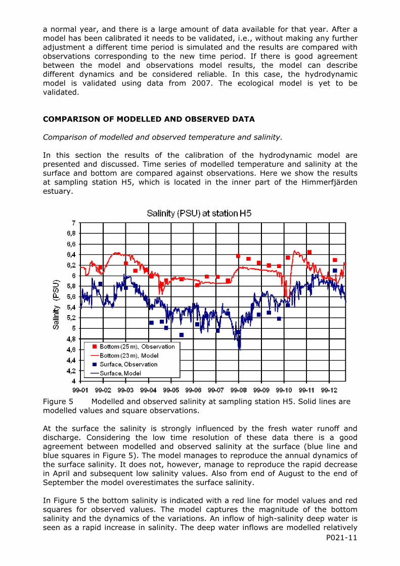
Figure 5 Modelled and observed salinity at sampling station H5. Solid lines are modelled values and square observations.

At the surface the salinity is strongly influenced by the fresh water runoff and discharge. Considering the low time resolution of these data there is a good agreement between modelled and observed salinity at the surface (blue line and blue squares in Figure 5). The model manages to reproduce the annual dynamics of the surface salinity. It does not, however, manage to reproduce the rapid decrease in April and subsequent low salinity values. Also from end of August to the end of September the model overestimates the surface salinity.

In Figure 5 the bottom salinity is indicated with a red line for model values and red squares for observed values. The model captures the magnitude of the bottom salinity and the dynamics of the variations. An inflow of high-salinity deep water is seen as a rapid increase in salinity. The deep water inflows are modelled relatively

P021-11

well except for the one at the end of July. The modelled inflow is not strong enough to increase the salinity to the observed values. During August and September the model salinities are a few tenths of PSU too low compared to the observations.

Figure 6 Modelled and observed temperature at sampling station H5. Solid lines are modelled values and square observations.

There is a good agreement between modelled and observed sea surface temperature (blue line and blue squares in Figure 6). This indicates that the heat exchange between the sea and atmosphere is correctly formulated in the model. The model has a tendency to underestimate the temperature during the spring and partly in the fall at the stations located in the inner part of the estuary. This may be due to the fact that the meteorological data used to force the model comes from an off-shore weather station and is thus not fully representative of the weather conditions in the inner part of the estuary.

There is generally a good agreement between modelled and observed bottom temperature (red line and red squares in Figure 6). The model shows warmer bottom water in August and September compared to the observations. This is probably due to a too weak inflow of cold and saline deep water in the model (compare with bottom salinity in Figure 5).

Figure 7 shows the surface and bottom temperature at station H4 located in the central part of the estuary (see map in Figure 1). This station is used to illustrate a problem occurring at several of the sampling stations. At these stations the modelled values are constant while the observations show seasonal variations. This is due to the computational cell used for the comparison being very deep in comparison to surrounding cells and therefore cut-off from their surroundings. In the model the location corresponding to the position of the sampling stations is like a shaft. In these shafts the water is rather stagnant and the water exchange very small. If the observed bottom temperature is compared with the modelled temperature at the upper edge of the shaft a much better agreement is obtained (see green curve in Figure 7 which is the modelled temperature at 18 m). The deepest model cell is not representative of the bottom conditions.

P021-12

Figure 7 Modelled and observed temperature at sampling station H4. Solid lines are modelled values and square observations. Once the calibration was completed the hydrodynamic model was validated. The hydrodynamic model was run without additional adjustment with forcing corresponding to year 2007 and the results were compared with observations from 2007. For the salinity there was generally a better agreement than for 1999, especially at the bottom. This may be due to 2007 being a less dynamic year with fewer deep water inflows. As for the temperature the agreement was as good as it was in 1999. The hydrodynamic model is therefore considered to be validated and good enough to be coupled with the ecological one. Comparison of modelled and observed biochemical variables Model results of chlorophyll-a, dissolved inorganic nitrogen, total-nitrogen, dissolved inorganic phosphorous, total-phosphorous and dissolved oxygen are compared with observation at sampling station H4, which is located in the central part of the Himmerfjärden estuary. The comparisons are carried out at the surface and at 15 m. The surface primary production is the dominant process while at 15 m the recycling processes play a dominant role as light levels are too low for any primary production to occur.

P021-13

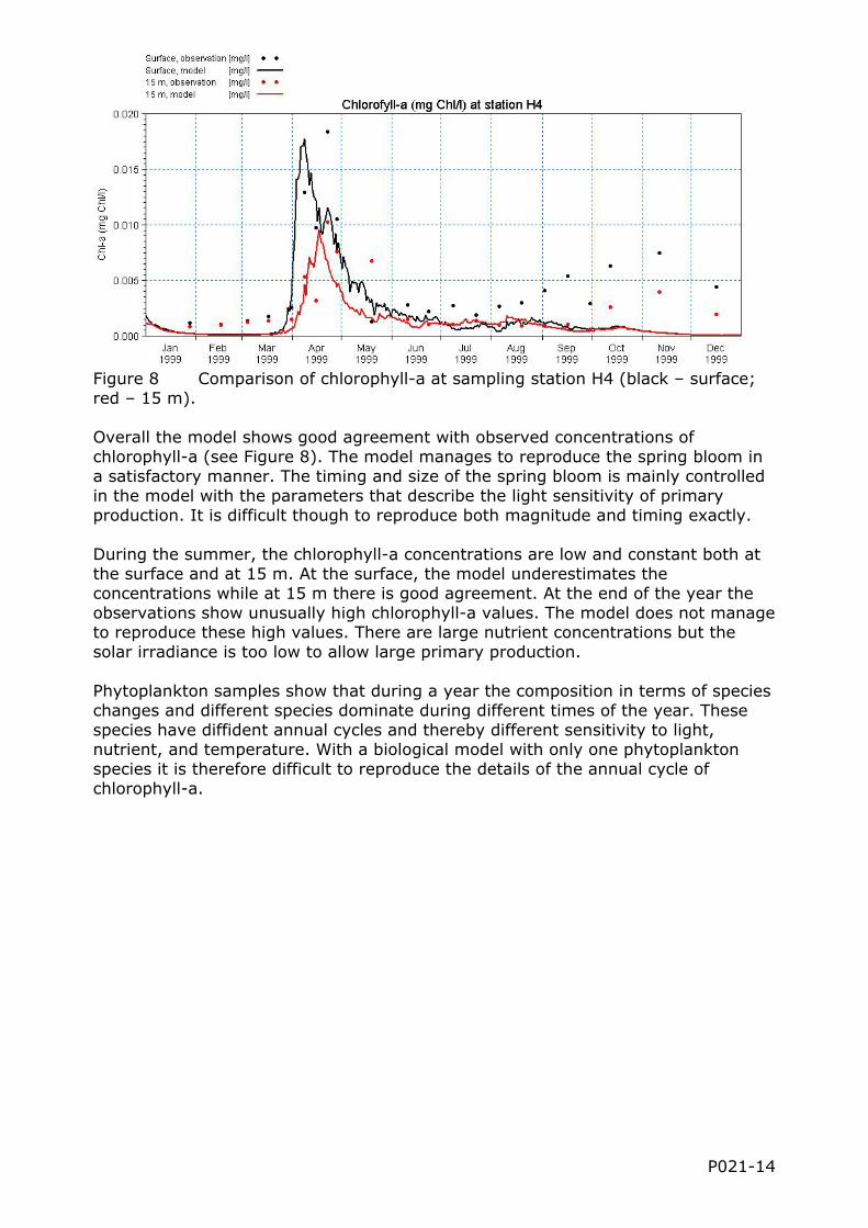
Figure 8 Comparison of chlorophyll-a at sampling station H4 (black – surface; red – 15 m). Overall the model shows good agreement with observed concentrations of chlorophyll-a (see Figure 8). The model manages to reproduce the spring bloom in a satisfactory manner. The timing and size of the spring bloom is mainly controlled in the model with the parameters that describe the light sensitivity of primary production. It is difficult though to reproduce both magnitude and timing exactly. During the summer, the chlorophyll-a concentrations are low and constant both at the surface and at 15 m. At the surface, the model underestimates the concentrations while at 15 m there is good agreement. At the end of the year the observations show unusually high chlorophyll-a values. The model does not manage to reproduce these high values. There are large nutrient concentrations but the solar irradiance is too low to allow large primary production. Phytoplankton samples show that during a year the composition in terms of species changes and different species dominate during different times of the year. These species have diffident annual cycles and thereby different sensitivity to light, nutrient, and temperature. With a biological model with only one phytoplankton species it is therefore difficult to reproduce the details of the annual cycle of chlorophyll-a.

P021-14

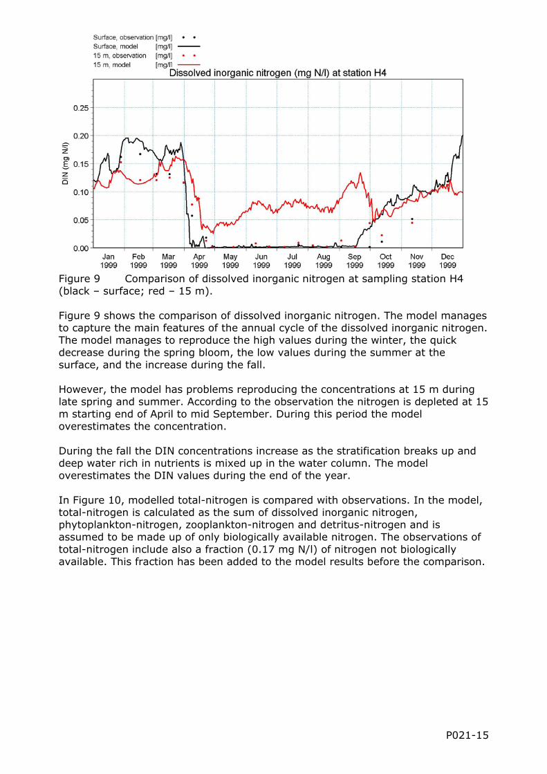
Figure 9 Comparison of dissolved inorganic nitrogen at sampling station H4 (black – surface; red – 15 m). Figure 9 shows the comparison of dissolved inorganic nitrogen. The model manages to capture the main features of the annual cycle of the dissolved inorganic nitrogen. The model manages to reproduce the high values during the winter, the quick decrease during the spring bloom, the low values during the summer at the surface, and the increase during the fall. However, the model has problems reproducing the concentrations at 15 m during late spring and summer. According to the observation the nitrogen is depleted at 15 m starting end of April to mid September. During this period the model overestimates the concentration. During the fall the DIN concentrations increase as the stratification breaks up and deep water rich in nutrients is mixed up in the water column. The model overestimates the DIN values during the end of the year. In Figure 10, modelled total-nitrogen is compared with observations. In the model, total-nitrogen is calculated as the sum of dissolved inorganic nitrogen, phytoplankton-nitrogen, zooplankton-nitrogen and detritus-nitrogen and is assumed to be made up of only biologically available nitrogen. The observations of total-nitrogen include also a fraction (0.17 mg N/l) of nitrogen not biologically available. This fraction has been added to the model results before the comparison.

P021-15

Figure 10 Comparison of total-nitrogen at sampling station H4 (black – surface; red – 15 m). At the surface the model manages to reproduce the annual cycle of total-nitrogen. The model captures e.g. the decrease after the spring bloom when organic material sinks out of the water column, the annual minimum during the summer and the increase during the fall when the sediment release inorganic nutrients. The problem at the surface is that the model underestimates the concentration the entire year. The underestimate is the worst during the summer when the difference between the model and observations is ca 0.15 mg N/l. At 15 m the situation is the opposite. The model concentrations of total-nitrogen are closer to the observation but the model does not manage to reproduce the dynamics of the annual cycle. During the summer the concentration of total-nitrogen does not decrease and during the fall/winter the concentration does not increase.

Figure 11 Comparison of dissolved oxygen at sampling station H4 (black – surface; red – 15 m).

P021-16

P021-17

The model manages to reproduce the annual cycle of dissolved oxygen (see Figure 11). Both the magnitude and variations calculated by the model agree well with observations. This means that the oxygen production and consumption, as well at the exchange with the atmosphere are well described in the model. Model values of dissolved inorganic phosphorous and total-phosphorous were also compared with observations (not shown). The performance of the ecological model in terms of phosphorous is very similar to the one for nitrogen. The issues are the same, e.g. the model also overestimates the concentration of inorganic phosphorous at 15 m during the summer. DISCUSSION AND CONCLUSIONS Hydrodynamic model The calibration and validation of the hydrodynamic model show that the model manages to capture the physical processes occurring in the Himmerfjärden estuary. The model manages to reproduce the dynamics of the salinity and temperature and thereby the water exchange. The hydrodynamic model confirms the picture obtained from the observations that the currents driven by density differences are important for the deep water. The results also show the importance of mixing for the deep water and the development of thermocline. It is also clear from the simulation the large impact the fresh water discharge has on the surface salinity and surface temperature. Nevertheless, the model shows some deficiencies, which are mainly due to two factors: 1) the low resolution in time of the fresh water discharge data, and 2) problems in describing mixing and inflow of deep water. When it comes to the fresh water discharge only monthly means are available which gives a very rough picture of how the discharge varies. This could be remedied by setting up a separate discharge model. However, it is uncertain if the effort would be worth it. This study focuses on the ecological processes in the estuary and typical time scales for the interesting ecological processes are slower than the time scales for the hydrodynamic processes. The issues with the deep water are closely related to the description of the bottom bathymetry. Firstly, it affects the comparison between model results and observations. What depth should be used for the comparison when the bottom depth of the model and observation differs? How should deep single cells isolated from their surrounding be treated? Secondly, deficiencies in the description of the bathymetry lead to error in sill depths and cross-sectional areas which affects the inflow of deep water. For example, if a sill depth is too shallow the deep water will not reach the inner basins of the estuary. The model bathymetry is most likely shallower than the real bathymetry. For example, at some of the sampling stations some of the deepest observations are deeper than the bottom depth according to the marine charts. This discrepancy in bottom depth results in the model underestimating the volume of the deep water. This has several consequences. For example, an inflow will fill up the bottom part of a basin faster, causing the inflow to end earlier than it should. This means that a smaller volume of cold and saline deep water from the Baltic Sea enters because there is simply not room for more. Also, if the model underestimates the volume of water in the domain, the quantity of substances in the water, such as nutrients, will also be underestimated. The model bathymetry is based on official marine charts.

P021-18

More detailed and accurate sounding data are available but were classified and thus not available for this study. Ecological model The ecological model manages to reproduce the main features of the annual cycle of the ecological state variables. Although there are some exceptions, the state variables have the right magnitude and the model captures the seasonal variations. At the surface, the dominant event is the spring bloom and the model does well in capturing both the timing and size of the spring bloom. Also the fast and large changes in phytoplankton and inorganic nutrients during the spring bloom are well described. Below the euphotic zone, where light is not available, the phytoplankton increase and the nutrients decrease as well during the spring bloom. These changes are not due to increased primary production as the light levels are too low at these depths. In the spring, the water column is well-mixed and mixing has an equalizing effect. Some of the phytoplankton biomass produced during the spring bloom is mixed downward the water column while the nutrients are mixed upward to make up to make up for losses at the surface. This is an example of how important it is to model both the hydrodynamic and ecological processes. The ecological model has some deficiencies. For example, during the summer months, the model overestimates the concentrations of the inorganic nutrients (nitrogen and phosphorus) below the euphotic zone. The ecological model needs to be improved so that it can better describe the ecological processes in Himmerfjärden. Based on the results of the calibration, the main issue with the ecological model is that it has difficulties reproducing the concentrations of dissolved inorganic nitrogen and phosphorus below the euphotic zone and near the bottom. At these depths sediment- and recycling-processes are of great importance. • Denitrification Denitrification turns nitrate (a component of dissolved inorganic nitrogen) into nitrogen gas (N2). As most phytoplankton species cannot take up nitrogen gas, denitrification leads to a loss of inorganic nitrogen (nutrient) in the water. In the current ecological model denitrification is not included. Although denitrification is not a dominant process in the Himmerfjärden estuary, including it would improve the model results and better describe the nitrogen dynamics in the estuary. • Sediment Processes During the summer months, after the biomass produced during the spring bloom has settled and reached the bottom, the sediments start releasing large amount of nitrogen and phosphorous. According to rough estimates (Blomkvist and Larsson, 1997), about 500 kg of phosphorus and 1000 kg of nitrogen are released from the sediments per day in Himmerfjärden during the summer months. These amounts correspond to 25 times the amount of phosphorus and 40% of the amount of nitrogen released daily from the sewage treatments plant. These figures give an indication of the importance of sediment processes. One of the major challenges when developing an ecological model is the parameterization of sediment processes. The current ecological model uses a simple formulation where a fraction of the phytoplankton and detritus that settles and reaches the bottom, is directly converted to dissolved inorganic nitrogen and phosphorous and returned to the water column. The sediment processes need to be modified in the ecological model, so that the right amount of nitrogen and phosphorus are released from sediments.

P021-19

• Total nitrogen and total phosphorus

The ecological model does not manage to properly reproduce the annual cycle of total-nitrogen and total-phosphorus. Preliminary analysis shows that this has to do mainly with how detritus and processes involving detritus are modelled. It is therefore necessary to look at how the model describes detritus, how the processes are formulated, and how model variables and parameters are related to observations.

Once the ecological model has been modified so that it describes the biological processes occurring in the Himmerfjärden estuary, the model can be used for scenario calculations such as the large-scale experiments taking place in Himmerfjärden.

REFERENCES

DHI (2009). DHI Eutrophication Model 1 – MIKE ECO Lab Template A Scientific Description. DHI Software, pp. 32.

DHI (2009). MIKE 21 & MIKE3 Flow Model FM Hydrodynamic and Transport Module Scientific Documentation. DHI Software, pp. 50.

Elmgren, Ragnar, & Larson, Ulf (ed.) (1997). Himmerfjärden: Förändringar i ett näringsbelastat kustekosystem i Östersjön. Naturvårdsverket (Swedish Environmental Protection Agency). Report 4565, pp. 197.

Engqvist, Anders, & Omstedt, Anders (1992). Water exchange and density structure in a multi-basin estuary. Continental Shelf Research , 12 (9), p. 1003-1026.

Liungman, Olof, Karlsson, Dick, & Sandberg, Johannes (2008). Adaptive coastal zone management: Technical Description Part 1- the Ecolab and MIKE 3 FLOW Model FM. Report prepared for the Swedish Environmental Proection Agency, pp. 65.

Sandberg, Johannes (2009). Adaptive coastal zone management: Technical Description: Part 2 - the ecological model - MIKE ECO Lab. Report prepared for the Swedish Environmental Proection Agency, pp. 62.