Hydrodynamic river modelling with D-Flow Flexible...

MSc thesis in Civil Engineering and Management

Hydrodynamic river modelling with

D-Flow Flexible Mesh

Case study of the side channel at Afferden and Deest

E.D.M. Ten Hagen

Hydrodynamic river modelling with D-Flow Flexible MeshCase study of the side channel at Afferden and Deest

MSc thesis in Civil Engineering and Management

Author: Erik ten HagenStudy: Civil Engineering and Management, University of TwenteStudent number: s1009230e-mail: [email protected]: September 18, 2014

Supervisors: Prof. Dr. S.J.M.H. HulscherUniversity of Twente, Department of Water Engineering and ManagementDr. J.J. WarminkUniversity of Twente, Department of Water Engineering and ManagementDr. F. HuthoffHKV – Lijn in Water, Department of Rivers and Coasts

3

DisclaimerThe research in this thesis was conducted using the new hydrodynamical simulation software D-FlowFlexible Mesh, developed at Deltares. It was still under development at the time of writing, and alsoafterwards. The used version was 1.1.100.34401. Since the software itself was still undergoing research, andalso documentation was limited, the results in this thesis are not always representative of the futureproduct version. Improvements are being made, but also good modeling practices have been learned by thestudent during this Masters project, which also has affected the results.

5

AbstractAccurate predictions of water levels play an important role in the management of flood safety. Nowadays, ithas become common practice to use multi-dimensional numerical hydrodynamic models for such purposes.Currently, WAQUA and Delft3D are standard tools in the Netherlands, which are based on a structuredcurvilinear grid. The curvilinear grid can follow large-scale topographical changes and uses similar gridresolution throughout the entire computational domain. Drawbacks of the structured curvilinear gridapproach are that staircase representation of closed boundaries is sometimes unavoidable, because gridcells are not aligned with the flow direction and in the inner bends of meandering rivers, gridlines maybecome focussed to unnecessarily small grid cells. To improve on these issues, Deltares is developing theunstructured-grid-based hydrodynamic model Flexible Mesh (also referred to as “D-Flow-FM”). Theunstructured grid approach enables the user to use a spatially variable grid resolution. By combiningcurvilinear grid cells with triangular grid cells, the modeller can increase grid resolution on the locationswhere, because of local topographical variations, it is most desired. In this study Flexible Mesh is tested andcompared with the structured grid based WAQUA and the possibilities of the unstructured mesh of FlexibleMesh are applied on a side channel at Afferden at Deest, where the WAQUA grid is considered to beinaccurate. The main objective of this research is:

Evaluate the performance (water levels, flow velocities and discharges) of Flexible Mesh by comparing with WAQUA and assess the sensitivity of the modelling results for the grid resolution in Flexible Mesh.

In the first step of the study the Flexible Mesh model is compared to the calibrated WAQUA model withfocus on the water levels, discharges and flow velocities. The water levels in the Flexible Mesh model arecomparable to the results of the water levels in the WAQUA model. For low discharges there is almost nodifference in the water level and for high discharges the water levels are about 12 centimeters higher in theFlexible Mesh model. The discharges over the floodplains and in the side channel are much smaller in theFlexible Mesh model. There are two important sources for the differences between WAQUA and FlexibleMesh. First, Flexible Mesh default uses a different, corrected formula for the Colebrook-White roughnesswhich results in a larger friction in Flexible Mesh and higher water levels. Second, the energy losses due toflow over weirs is modelled different in Flexible Mesh, which results in higher water levels in Flexible Meshand lower discharges over the floodplain and in the side channel at Afferden and Deest.

In the second step local grid refinement was applied at Afferden and Deest to the main channel of the Waaland to the side channel. The grid refinement of the main channel of the Waal showed no clear effectsbetween consecutive grid refinements. The local grid refinement was also applied for the side channel,where the original grid is assumed to schematize the side channel inaccurate. The difference with thereference grid is maximal for the schematization with the largest refined side channel. However, the effectof grid refinement decreased at higher grid resolutions which indicates convergence of the model results.After the grid was refined four times, the results were hardly affected by a grid refinement anymore.Therefore, convergence seems to be reached around the four times refined side channel. Thecomputational time increases because of grid refinement. For high grid resolutions, the time step has to bedecreased in order to meet the model condition stability (default Courant number < 0,7). Grid refinement isefficient when model results are not yet converged, so further refinement has still effect on the modelresults, and computational time is still acceptable.

The results of this study show potential for application of local grid refinements with the unstructured gridof D-Flow Flexible Mesh for complex geometries. The accuracy of the computation of the flow in the sidechannel seems to be improved by the local grid refinement. However, further research is required to assessthe accuracy of Flexible Mesh.

7

Samenvatting (Dutch)Nauwkeurige voorspellingen van waterstanden spelen een belangrijke rol in het beheer van waterveiligheid.Tegenwoordig is het gebruikelijk geworden om multidimensionale numerieke hydrodynamische modellen tegebruiken voor deze doeleinden. Momenteel zijn WAQUA en Delft3D, die zijn gebaseerd op eengestructureerd curvilineair rooster, gebruikelijke instrumenten in Nederland. Het curvilineaire rooster kangroot schalige topographise verschillen goed weergeven en gebruikt een overeenkomstige rooster resolutieover het gehele rekenkundige domein. Nadelen van het curvilineaire rooster is dat trapjes weergave vangesloten grenzen soms niet voorkombaar is, doordat het rooster niet de stroomrichting volgt en dat in debinnenbochten van meanderende rivieren roosterlijnen gefocust worden tot onnodig kleine rooster cellen.Om op deze punten te verbeteren ontwikkeld Deltares de op een ongestructureerd rooster gebaseerdehydrodynamische model D-Flow Flexible Mesh. De ongestructureerde rooster benadering maakt hetmogelijk voor de gebruiker om een ruimtelijke variabele rooster resulutie te gebruiken. Door curvilineaireen driehoekige rooster cellen te combineren kan de modelleur de rooster resolutie verhogen op de locatieswaar dat het meest gewenst is. In deze studie is Flexible Mesh getest en vergeleken met de op eengestructureerde rooster gebaseerde WAQUA en de mogelijkheden van het ongestructureerde rooster vanFlexible Mesh zijn toegepast op de nevengeul bij Afferden en Deest, waar het WAQUA rooster nietnauwkeurig wordt geacht. Het hoofddoel van dit onderzoek is:

Evalueer de prestaties (waterstanden, stroomsnelheden en afvoeren) van Flexible Mesh door te vergelijken met WAQUA en beoordeeld de gevoeligheid van de model resultaten voor de rooster resolutie in Flexible Mesh.

In de eerste stap van de studie is het Flexible Mesh model vergeleken met het gekalibreerde WAQUA modelwaarbij is gefocust op de waterstanden, afvoeren en stroomsnelheden. De waterstanden in het FlexibleMesh model zijn vergelijkbaar met de resultaten in het WAQUA model. For lage afvoeren zijn er bijna geenverschillen en voor hoge afvoeren zijn de waterstanden in het Flexible Mesh model ongeveer 10 centimeterhoger. De afvoeren over het winterbed en door de nevengeul zijn veel lager in het Flexible Mesh model. Erzijn twee belangrijke bronnen voor de verschillen tussen het WAQUA en Flexible Mesh model. Ten eerstewordt er in het Flexible Mesh model standaard een andere, gecorrigeerde formule gebruikt voor deColebrook-White ruwheid, wat resulteert in een hogere frictie in Flexible Mesh en hogere waterstanden.Ten tweede wordt het energieverlies door stroming over overlaten anders gemodelleerd in Flexible Mesh,wat resulteert in hogere waterstanden en lager afvoeren over het winterbed en door de nevengeul bijAfferden en Deest.

In het vervolg is lokale roosterverfijning toegepast op op de hoofdgeul van de Waal en de nevengeul bijAfferden en Deest. Bij de roosterverfijning van de hoofdgeul zijn geen eenduidige effecten geconstateerdtussen opeenvolgende roosterverfijningen. De roosterverfijning is ook toegepast op de nevengeul. Hetverschil met het originele grid is maximaal voor de schematizatie met de hoogste rooster resolutie in denevengeul. Echter het effect van de roosterverfijning is veel kleiner voor het rooster met een hoge resolutiewat er op wijst dat model resultaten zijn geconverteerd. Nadat het rooster in de nevengeul vier maal wasverfijnd, bleek dat de modelresultaten nauwelijks nog werden beïnvloed door een roosterverfijning en dusconvergentie van de modelresultaten leek te zijn bereikt bij een vier maal verfijnde nevengeul. The rekentijdnam toe door de roosterverfijning. Voor hoge rooster resoluties moest de tijdstap verlaagd worden om tevoldoen aan het criterium voor model stabiliteit (standaard Courant getal < 0,7). Daarom is roosterverfijningmet name efficient wanneer modelresultaten nog niet zijn geconverteerd en dus verdere verfijning nogeffect heeft op de resultaten en rekentijd acceptabel blijft.

De resultaten in deze studie laten potentieel zien voor de toepassing van lokale rooster verfijningen met hetongestructureerde rooster van D-Flow Flexible Mesh for comlexe geometrieën. The nauwkeurigheid van deberekening van de stroming in de nevengeul lijkt te zijn verbeterd door de rooster verfijning. Echter, verderonderzoek is nodig om the nauwkeurigheid van Flexible Mesh te bepalen.

9

AcknowledgementsThis Master Thesis presents the results of the research I carried out in the past six months. It is the last stepin finishing my master Civil Engineering & Management with the specialization Water Engineering &Management at the University of Twente. In this research I carried out a testcase for the unstructuredhydrodynamic model D-Flow Flexible Mesh, which is currently under development. I conducted theresearch at HKV lijn in water.

First I would like to thank everyone who helped me at HKV lijn in water, but in particularly Andries andJoana for support for setup of the models and providing feedback. Special thanks go to Andries for makingsimulations on the compute cluster possible. I would also thank Aukje, Arthur, Herman, Robert and Willemof Deltares, who supported me when I had trouble with D-Flow Flexible Mesh and kindly helped to solvethose troubles. Further, thanks go to Tijmen of Rijkswaterstaat Oost-Nederland, who provided the WAQUAmodel and data of the Rhinemodel. I would also thank the members of my graduation committee, Suzanne,Jord and Fredrik for providing valuable feedback.

Last but not least, I would thank my family, especially my parents Herman and Greta for supporting meduring the entire study.

Erik ten Hagen

Winterswijk, September 2014

11

Table of contentsDisclaimer...............................................................................................................................................................5Abstract...................................................................................................................................................................7Samenvatting (Dutch).............................................................................................................................................9Acknowledgements..............................................................................................................................................11List of symbols......................................................................................................................................................151Introduction........................................................................................................................................................17

1.1Hydrodynamic models................................................................................................................................171.2Computational grid.....................................................................................................................................181.3Numerical solution.....................................................................................................................................201.4Differences numerical solution...................................................................................................................211.5Research objectives....................................................................................................................................221.6Case Afferden-Deest...................................................................................................................................221.7Thesis outline.............................................................................................................................................24

2Analysis differences WAQUA – Flexible Mesh....................................................................................................252.1Model differences WAQUA – Flexible Mesh...............................................................................................25

2.1.1Colebrook-White formula..................................................................................................................252.1.2Conveyance........................................................................................................................................262.1.3Energy losses by weirs........................................................................................................................262.1.4Thin dams...........................................................................................................................................26

2.2Rectangular testmodel...............................................................................................................................262.2.1Method...............................................................................................................................................262.2.2Results................................................................................................................................................28

2.3Testmodel Waal..........................................................................................................................................292.3.1Method...............................................................................................................................................292.3.2Results................................................................................................................................................30

2.4Conclusions testmodels..............................................................................................................................323Methodology of comparison and grid refinement.............................................................................................33

3.1Comparison Flexible Mesh – WAQUA.........................................................................................................333.1.1Waal without side channel.................................................................................................................333.1.2Waal with side channel......................................................................................................................34

3.2Grid refinement..........................................................................................................................................353.2.1Model setup.......................................................................................................................................353.2.2Grid refinement main channel...........................................................................................................363.2.3Grid refinement side channel (not aligned).......................................................................................363.2.4Grid refinement side channel (aligned)..............................................................................................36

4Results................................................................................................................................................................394.1Comparison Flexible Mesh – WAQUA.........................................................................................................39

4.1.1Waal without side channel.................................................................................................................394.1.2Waal with side channel......................................................................................................................41

4.2Grid refinement..........................................................................................................................................444.2.1Waal refinement.................................................................................................................................444.2.2Side channel refinement (not aligned)...............................................................................................464.2.3Side channel refinement (aligned).....................................................................................................47

4.3Computation time......................................................................................................................................505Discussion...........................................................................................................................................................51

5.1Interpretation results comparison..............................................................................................................515.2Interpretation results grid refinement........................................................................................................525.3Practical application of Flexible Mesh........................................................................................................53

6Conclusions and recommendations....................................................................................................................556.1Conclusions.................................................................................................................................................556.2Recommendations......................................................................................................................................56

Literature..............................................................................................................................................................59

13

List of symbols

B Channel width [m]c Celerity [m s-1]C Chézy value [m1/2 s-1]Cf Bed friction coefficient [-]F Driving forces [-]f Coriolis parameter [rad s-1]g Gravitational acceleration [m s-2]h Water depth [m]h0 Hydraulic radius [m]ib Bed level gradient [-]Ks Nikuradse roughness [m]Q Discharge [m3 s-1]T Lateral stresses [N m-2]u Flow velocity in x-direction [m s-1]v Flow velocity in y-direction [m s-1]

ζ Water elevation above reference plane [m]κ Von Karman's constant [-]ν Kinematic viscosity [m2 s-1]ρ Density of water [kg m-3]ρ0 Mean density of water [kg m-3]τb Bed shear stress [N m-2]φ Geographic latitude [°]Ω Rotation of earth [rad s-1]

15

1 IntroductionAccurate predictions of water levels play an important role in the management of flood safety. Nowadays, ithas become common practice to use multi-dimensional numerical hydrodynamic models for such purposes.Currently, two model types are the standard tools in the Netherlands, namely WAQUA/TRIWAQ[Rijkswaterstaat, 2012] and Delft3D [Deltares, 2014]. WAQUA and Delft3D are both based on structuredcurvilinear grids, which can follow large-scale topographical changes and uses similar grid resolutionthroughout the entire computational domain. However, to accurately resolve flow and transport processes,a locally refined grid resolution is desirable. Currently, Deltares is developing the software system D-FlowFlexible Mesh (hereafter to be called Flexible Mesh), which is based on an unstructured grid. Theunstructured grid approach in Flexible Mesh enables the user to use a spatially variable grid resolution. AsFlexible Mesh is still under development, the model needs to be tested and validated. In commission ofDeltares, multiple testcases are carried out. In this research, a testcase for Flexible Mesh is described. Theproject 'Herinrichting Afferdense en Deestse Waarden' along the river Waal, where a side channel will belandscaped, is subject of the testcase

This chapter introduces the principles of hydrodynamic models and the numerical approach. Thedifferences between commonly used hydrodynamic models and Flexible Mesh are discussed. The objectiveof this research and related research questions are presented. Finally the case study 'Project herinrichtingAfferdense and Deestse Waarden' will be described and the outline of this thesis is given.

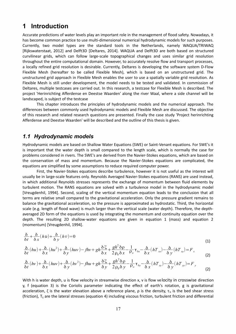
1.1 Hydrodynamic modelsHydrodynamic models are based on Shallow Water Equations (SWE) or Saint-Venant equations. For SWE's itis important that the water depth is small compared to the length scale, which is normally the case forproblems considered in rivers. The SWE's are derived from the Navier-Stokes equations, which are based onthe conservation of mass and momentum. Because the Navier-Stokes equations are complicated, theequations are simplified by some assumptions to reduce required computer power.

First, the Navier-Stokes equations describe turbulence, however it is not useful as the interest willusually be in large-scale features only. Reynolds Averaged Navier-Stokes equations (RANS) are used instead,in which additional Reynolds stresses represents the exchange of momentum between fluid elements byturbulent motion. The RANS equations are solved with a turbulence model in the hydrodynamic model[Vreugdenhil, 1994]. Second, scaling of the vertical momentum equation leads to the conclusion that allterms are relative small compared to the gravitational acceleration. Only the pressure gradient remains tobalance the gravitational acceleration, so the pressure is approximated as hydrostatic. Third, the horizontalscale (e.g. length of flood wave) is much larger than the vertical scale (water depth). Therefore, the depth-averaged 2D form of the equations is used by integrating the momentum and continuity equation over thedepth. The resulting 2D shallow-water equations are given in equation 1 (mass) and equation 2(momentum) [Vreugdenhil, 1994].

δδt

+ δδ x

(hu)+ δδ y

(hv )=0(1)

δδt

(hu)+ δδ x

(hu2)+ δ

δ y(huv )− fhv+ gh

δ ζ

δ x+gh2

δρ

2ρ0 δ x−

1ρo

τbx−δδ x

(hT xx)−δ

δ y(hT xy)=F x

(2)

δδt

(hv )+ δδ x

(huv)+ δδ y

(hv2)− fhu+gh

δζ

δ y+gh2

δρ

2ρ0 δ y−

1ρo

τby−δ

δ x(hT xy)−

δδ y

(hT yy)=F y

(2)

With h is water depth, u is flow velocity in streamwise direction x, v is flow ve locity in crosswise directiony, f (equation 3) is the Coriolis parameter indicating the effect of earth's rotation, g is gravitationalacceleration, ζ is the water elevation above a reference plane, ρ is the density, τ b is the bed shear stress(friction), Tij are the lateral stresses (equation 4) including viscous friction, turbulent friction and differential

17

advection and F are driving forces (e.g. wind stress). The lateral stresses and driving forces may bedisregarded. Further, for the bottom stress the simplest expression might be assumed, resulting in thestandard SWE's.

f =2Ω sinϕ (3)

T ij=1h∫0

h

(ν(δ uiδ x j

+δu jδ x i

)−ui ' u j '+(ui−u i)(u j−u j))dz (4)

With Ω is the angular rate of revolution, φ is the geographic latitude and ν is the viscosity.

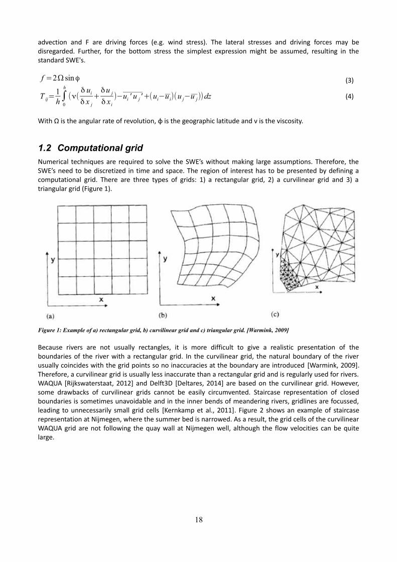
1.2 Computational gridNumerical techniques are required to solve the SWE’s without making large assumptions. Therefore, theSWE’s need to be discretized in time and space. The region of interest has to be presented by defining acomputational grid. There are three types of grids: 1) a rectangular grid, 2) a curvilinear grid and 3) atriangular grid (Figure 1).

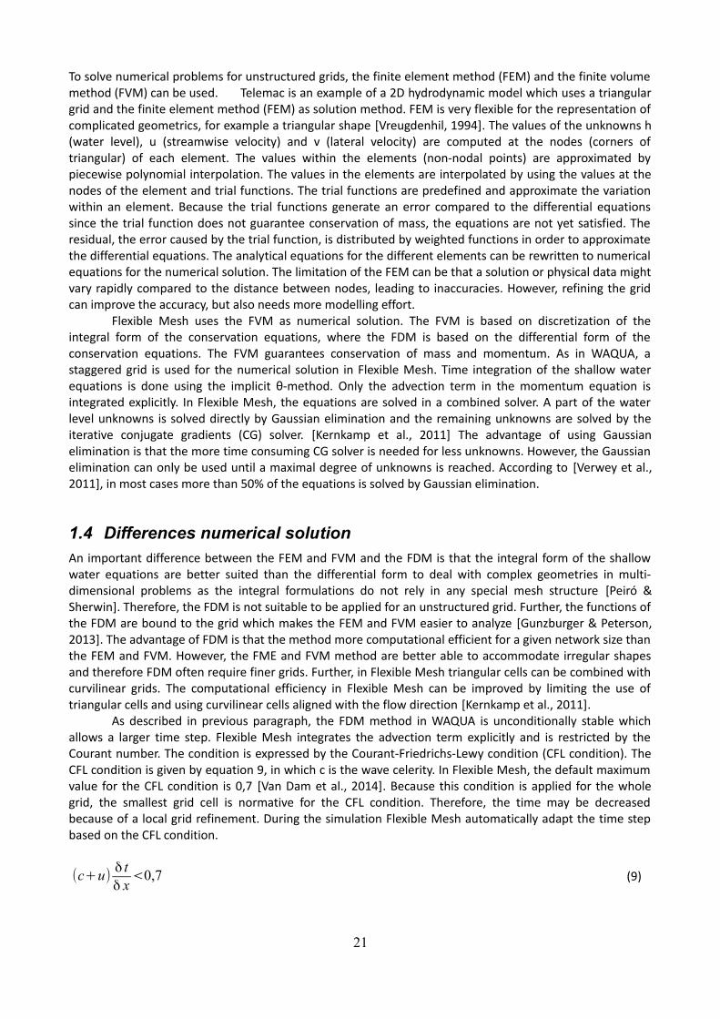
Because rivers are not usually rectangles, it is more difficult to give a realistic presentation of theboundaries of the river with a rectangular grid. In the curvilinear grid, the natural boundary of the riverusually coincides with the grid points so no inaccuracies at the boundary are introduced [Warmink, 2009].Therefore, a curvilinear grid is usually less inaccurate than a rectangular grid and is regularly used for rivers.WAQUA [Rijkswaterstaat, 2012] and Delft3D [Deltares, 2014] are based on the curvilinear grid. However,some drawbacks of curvilinear grids cannot be easily circumvented. Staircase representation of closedboundaries is sometimes unavoidable and in the inner bends of meandering rivers, gridlines are focussed,leading to unnecessarily small grid cells [Kernkamp et al., 2011]. Figure 2 shows an example of staircaserepresentation at Nijmegen, where the summer bed is narrowed. As a result, the grid cells of the curvilinearWAQUA grid are not following the quay wall at Nijmegen well, although the flow velocities can be quitelarge.

18

Figure 1: Example of a) rectangular grid, b) curvilinear grid and c) triangular grid. [Warmink, 2009]

Increasingly more models use a triangular grid, like Telemac [EDF-R&D, 2013] and MIKE 21 [DHI,2011]. The advantage of a triangular grid is that it is more flexible in the representation of the mesh,because the mesh can be locally refined. However, the unstructured grid requires another numericalsolution method. According to [Garcia, 2008], the grid refinement flexibility is obtained at the price ofcomputational efficiency, because the used numerical method for the structured grid is computational moreefficient.

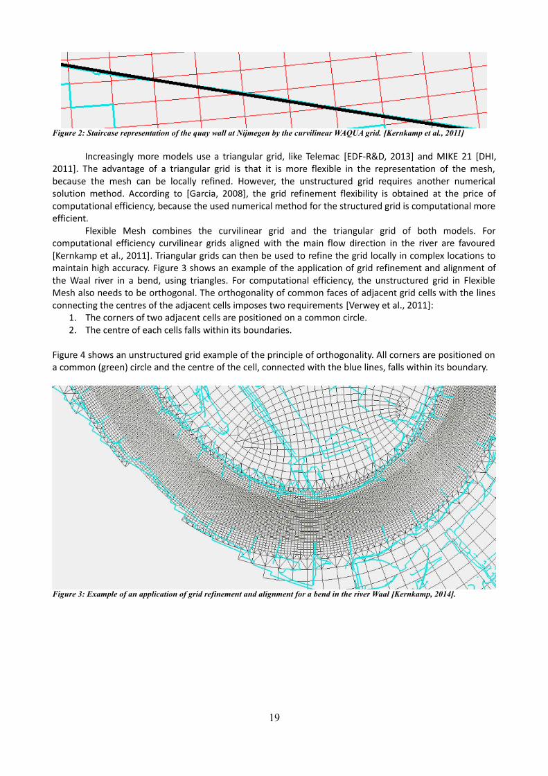
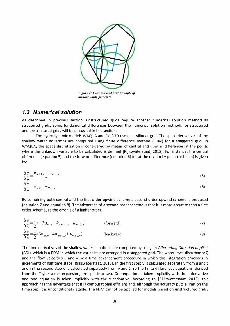
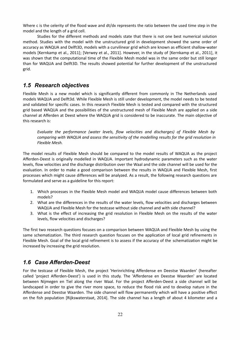
Flexible Mesh combines the curvilinear grid and the triangular grid of both models. Forcomputational efficiency curvilinear grids aligned with the main flow direction in the river are favoured[Kernkamp et al., 2011]. Triangular grids can then be used to refine the grid locally in complex locations tomaintain high accuracy. Figure 3 shows an example of the application of grid refinement and alignment ofthe Waal river in a bend, using triangles. For computational efficiency, the unstructured grid in FlexibleMesh also needs to be orthogonal. The orthogonality of common faces of adjacent grid cells with the linesconnecting the centres of the adjacent cells imposes two requirements [Verwey et al., 2011]:

1. The corners of two adjacent cells are positioned on a common circle.2. The centre of each cells falls within its boundaries.

Figure 4 shows an unstructured grid example of the principle of orthogonality. All corners are positioned ona common (green) circle and the centre of the cell, connected with the blue lines, falls within its boundary.

19

Figure 3: Example of an application of grid refinement and alignment for a bend in the river Waal [Kernkamp, 2014].

Figure 2: Staircase representation of the quay wall at Nijmegen by the curvilinear WAQUA grid. [Kernkamp et al., 2011]

1.3 Numerical solutionAs described in previous section, unstructured grids require another numerical solution method asstructured grids. Some fundamental differences between the numerical solution methods for structuredand unstructured grids will be discussed in this section.

The hydrodynamic models WAQUA and Delft3D use a curvilinear grid. The space derivatives of theshallow water equations are computed using finite difference method (FDM) for a staggered grid. InWAQUA, the space discretization is considered by means of central and upwind differences at the pointswhere the unknown variable to be calculated is defined [Rijkswaterstaat, 2012]. For instance, the centraldifference (equation 5) and the forward difference (equation 6) for at the u-velocity point (cell m, n) is givenby:

δuδζ

=um+1,n−um−1, n

2(5)

δuδζ

=um+1, n−um , n (6)

By combining both central and the first order upwind scheme a second order upwind scheme is proposed(equation 7 and equation 8). The advantage of a second order scheme is that it is more accurate than a firstorder scheme, as the error is of a higher order.

δuδζ

=12(−3um ,n+4um+1,n−um+2, n) (forward) (7)

δuδζ

=12(3um ,n−4um+1,n+um+2,n) (backward) (8)

The time derivatives of the shallow water equations are computed by using an Alternating Direction Implicit(ADI), which is a FDM in which the variables are arranged in a staggered grid. The water level disturbance ζand the flow velocities u and v by a time advancement procedure in which the integration proceeds inincrements of half time steps [Rijkswaterstaat, 2013]. In the first step v is calculated separately from u and ζand in the second step u is calculated separately from v and ζ. So the finite differences equations, derivedfrom the Taylor series expansion, are split into two. One equation is taken implicitly with the x-derivativeand one equation is taken implicitly with the y-derivative. According to [Rijkswaterstaat, 2013], thisapproach has the advantage that it is computational efficient and, although the accuracy puts a limit on thetime step, it is unconditionally stable. The FDM cannot be applied for models based on unstructured grids.

20

Figure 4: Unstructured grid example of orthogonality principle.

To solve numerical problems for unstructured grids, the finite element method (FEM) and the finite volumemethod (FVM) can be used. Telemac is an example of a 2D hydrodynamic model which uses a triangulargrid and the finite element method (FEM) as solution method. FEM is very flexible for the representation ofcomplicated geometrics, for example a triangular shape [Vreugdenhil, 1994]. The values of the unknowns h(water level), u (streamwise velocity) and v (lateral velocity) are computed at the nodes (corners oftriangular) of each element. The values within the elements (non-nodal points) are approximated bypiecewise polynomial interpolation. The values in the elements are interpolated by using the values at thenodes of the element and trial functions. The trial functions are predefined and approximate the variationwithin an element. Because the trial functions generate an error compared to the differential equationssince the trial function does not guarantee conservation of mass, the equations are not yet satisfied. Theresidual, the error caused by the trial function, is distributed by weighted functions in order to approximatethe differential equations. The analytical equations for the different elements can be rewritten to numericalequations for the numerical solution. The limitation of the FEM can be that a solution or physical data mightvary rapidly compared to the distance between nodes, leading to inaccuracies. However, refining the gridcan improve the accuracy, but also needs more modelling effort.

Flexible Mesh uses the FVM as numerical solution. The FVM is based on discretization of theintegral form of the conservation equations, where the FDM is based on the differential form of theconservation equations. The FVM guarantees conservation of mass and momentum. As in WAQUA, astaggered grid is used for the numerical solution in Flexible Mesh. Time integration of the shallow waterequations is done using the implicit θ-method. Only the advection term in the momentum equation isintegrated explicitly. In Flexible Mesh, the equations are solved in a combined solver. A part of the waterlevel unknowns is solved directly by Gaussian elimination and the remaining unknowns are solved by theiterative conjugate gradients (CG) solver. [Kernkamp et al., 2011] The advantage of using Gaussianelimination is that the more time consuming CG solver is needed for less unknowns. However, the Gaussianelimination can only be used until a maximal degree of unknowns is reached. According to [Verwey et al.,2011], in most cases more than 50% of the equations is solved by Gaussian elimination.

1.4 Differences numerical solutionAn important difference between the FEM and FVM and the FDM is that the integral form of the shallowwater equations are better suited than the differential form to deal with complex geometries in multi-dimensional problems as the integral formulations do not rely in any special mesh structure [Peiró &Sherwin]. Therefore, the FDM is not suitable to be applied for an unstructured grid. Further, the functions ofthe FDM are bound to the grid which makes the FEM and FVM easier to analyze [Gunzburger & Peterson,2013]. The advantage of FDM is that the method more computational efficient for a given network size thanthe FEM and FVM. However, the FME and FVM method are better able to accommodate irregular shapesand therefore FDM often require finer grids. Further, in Flexible Mesh triangular cells can be combined withcurvilinear grids. The computational efficiency in Flexible Mesh can be improved by limiting the use oftriangular cells and using curvilinear cells aligned with the flow direction [Kernkamp et al., 2011].

As described in previous paragraph, the FDM method in WAQUA is unconditionally stable whichallows a larger time step. Flexible Mesh integrates the advection term explicitly and is restricted by theCourant number. The condition is expressed by the Courant-Friedrichs-Lewy condition (CFL condition). TheCFL condition is given by equation 9, in which c is the wave celerity. In Flexible Mesh, the default maximumvalue for the CFL condition is 0,7 [Van Dam et al., 2014]. Because this condition is applied for the wholegrid, the smallest grid cell is normative for the CFL condition. Therefore, the time may be decreasedbecause of a local grid refinement. During the simulation Flexible Mesh automatically adapt the time stepbased on the CFL condition.

(c+u)δ tδ x

<0,7 (9)

21

Where c is the celerity of the flood wave and dt/dx represents the ratio between the used time step in themodel and the length of a grid cell.

Studies for the different methods and models state that there is not one best numerical solutionmethod. Studies with the model with the unstructured grid in development showed the same order ofaccuracy as WAQUA and Delft3D, models with a curvilinear grid which are known as efficient shallow-watermodels [Kernkamp et al., 2011]; [Verwey et al., 2011]. However, in the study of [Kernkamp et al., 2011], itwas shown that the computational time of the Flexible Mesh model was in the same order but still longerthan for WAQUA and Delft3D. The results showed potential for further development of the unstructuredgrid.

1.5 Research objectivesFlexible Mesh is a new model which is significantly different from commonly in The Netherlands usedmodels WAQUA and Delft3d. While Flexible Mesh is still under development, the model needs to be testedand validated for specific cases. In this research Flexible Mesh is tested and compared with the structuredgrid based WAQUA and the possibilities of the unstructured mesh of Flexible Mesh are applied on a sidechannel at Afferden at Deest where the WAQUA grid is considered to be inaccurate. The main objective ofthis research is:

Evaluate the performance (water levels, flow velocities and discharges) of Flexible Mesh by comparing with WAQUA and assess the sensitivity of the modelling results for the grid resolution in Flexible Mesh.

The model results of Flexible Mesh should be compared to the model results of WAQUA as the projectAfferden-Deest is originally modelled in WAQUA. Important hydrodynamic parameters such as the waterlevels, flow velocities and the discharge distribution over the Waal and the side channel will be used for theevaluation. In order to make a good comparison between the results in WAQUA and Flexible Mesh, firstprocesses which might cause differences will be analyzed. As a result, the following research questions areformulated and serve as a guideline for this report:

1. Which processes in the Flexible Mesh model and WAQUA model cause differences between bothmodels?

2. What are the differences in the results of the water levels, flow velocities and discharges betweenWAQUA and Flexible Mesh for the testcase without side channel and with side channel?

3. What is the effect of increasing the grid resolution in Flexible Mesh on the results of the waterlevels, flow velocities and discharges?

The first two research questions focuses on a comparison between WAQUA and Flexible Mesh by using thesame schematization. The third research question focuses on the application of local grid refinements inFlexible Mesh. Goal of the local grid refinement is to assess if the accuracy of the schematization might beincreased by increasing the grid resolution.

1.6 Case Afferden-DeestFor the testcase of Flexible Mesh, the project 'Herinrichting Afferdense en Deestse Waarden' (hereaftercalled 'project Afferden-Deest') is used in this study. The 'Afferdense en Deestse Waarden' are locatedbetween Nijmegen en Tiel along the river Waal. For the project Afferden-Deest a side channel will belandscaped in order to give the river more space, to reduce the flood risk and to develop nature in theAfferdense and Deestse Waarden. The side channel will flow permanently which will have a positive effecton the fish population [Rijkswaterstaat, 2014]. The side channel has a length of about 4 kilometer and a

22

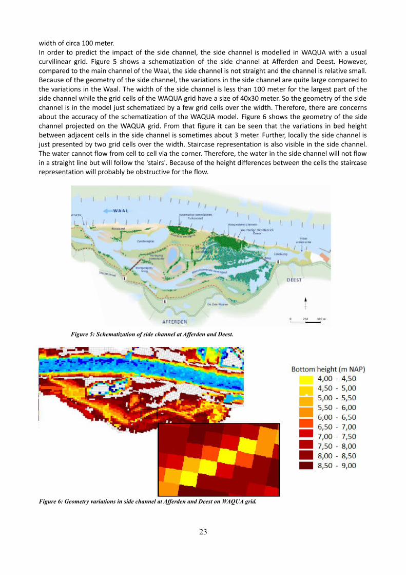
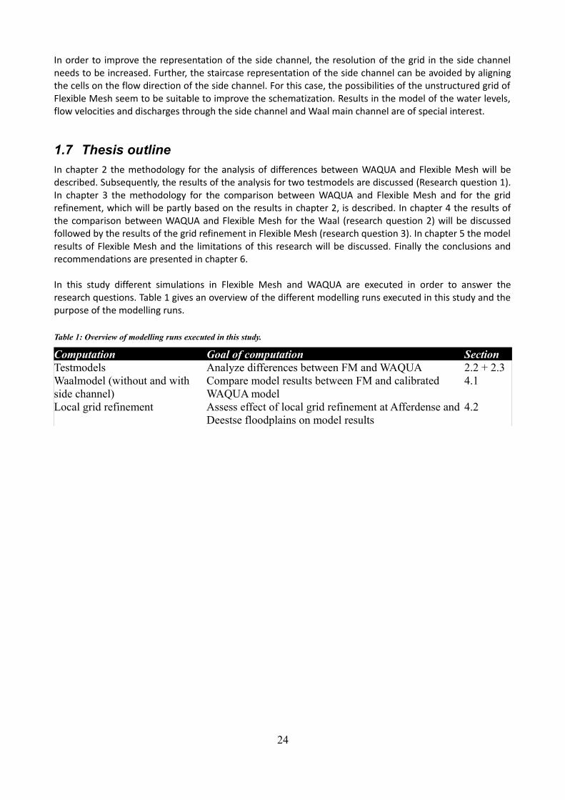
width of circa 100 meter. In order to predict the impact of the side channel, the side channel is modelled in WAQUA with a usualcurvilinear grid. Figure 5 shows a schematization of the side channel at Afferden and Deest. However,compared to the main channel of the Waal, the side channel is not straight and the channel is relative small.Because of the geometry of the side channel, the variations in the side channel are quite large compared tothe variations in the Waal. The width of the side channel is less than 100 meter for the largest part of theside channel while the grid cells of the WAQUA grid have a size of 40x30 meter. So the geometry of the sidechannel is in the model just schematized by a few grid cells over the width. Therefore, there are concernsabout the accuracy of the schematization of the WAQUA model. Figure 6 shows the geometry of the sidechannel projected on the WAQUA grid. From that figure it can be seen that the variations in bed heightbetween adjacent cells in the side channel is sometimes about 3 meter. Further, locally the side channel isjust presented by two grid cells over the width. Staircase representation is also visible in the side channel.The water cannot flow from cell to cell via the corner. Therefore, the water in the side channel will not flowin a straight line but will follow the 'stairs'. Because of the height differences between the cells the staircaserepresentation will probably be obstructive for the flow.

23

Figure 5: Schematization of side channel at Afferden and Deest.

Figure 6: Geometry variations in side channel at Afferden and Deest on WAQUA grid.

In order to improve the representation of the side channel, the resolution of the grid in the side channelneeds to be increased. Further, the staircase representation of the side channel can be avoided by aligningthe cells on the flow direction of the side channel. For this case, the possibilities of the unstructured grid ofFlexible Mesh seem to be suitable to improve the schematization. Results in the model of the water levels,flow velocities and discharges through the side channel and Waal main channel are of special interest.

1.7 Thesis outlineIn chapter 2 the methodology for the analysis of differences between WAQUA and Flexible Mesh will bedescribed. Subsequently, the results of the analysis for two testmodels are discussed (Research question 1).In chapter 3 the methodology for the comparison between WAQUA and Flexible Mesh and for the gridrefinement, which will be partly based on the results in chapter 2, is described. In chapter 4 the results ofthe comparison between WAQUA and Flexible Mesh for the Waal (research question 2) will be discussedfollowed by the results of the grid refinement in Flexible Mesh (research question 3). In chapter 5 the modelresults of Flexible Mesh and the limitations of this research will be discussed. Finally the conclusions andrecommendations are presented in chapter 6.

In this study different simulations in Flexible Mesh and WAQUA are executed in order to answer theresearch questions. Table 1 gives an overview of the different modelling runs executed in this study and thepurpose of the modelling runs.

Table 1: Overview of modelling runs executed in this study.

Computation Goal of computation SectionTestmodels Analyze differences between FM and WAQUA 2.2 + 2.3Waalmodel (without and with side channel)

Compare model results between FM and calibrated WAQUA model

4.1

Local grid refinement Assess effect of local grid refinement at Afferdense and Deestse floodplains on model results

4.2

24

2 Analysis differences WAQUA – Flexible MeshBefore working on model simulations for the testcase, first the WAQUA and Flexible Mesh models areanalyzed for basic model cases. The goal of this analysis is to observe which processes may cause largedifference between WAQUA and Flexible Mesh. Besides it will give a better understanding of the model, thisanalysis will be used to choose appropriate input for the other parts of the research. First, an outline ofimportant differences in model settings between WAQUA and Flexible Mesh will be given which mightcause differences in the results. Then the method for this analysis will be described. Finally results will beshown for a basic case and a more realistic case of a part of the Waal. Table 2 gives an overview of thedifferent modelling runs of testmodels executed in chapter 2 and the purpose of the modelling runs.

Table 2: Overview of testmodels executed in chapter 2.

Computation Goal of computation SectionRectangular testmodel Analyze differences between FM, WAQUA and

analytical estimation for model with uniform roughness2.2

Testmodel Waal (uniform roughness)

Analyze differences between FM and WAQUA for model with uniform roughness

2.3

Testmodel Waal (spatial variable roughness)

Analyze differences between FM and WAQUA for model roughness defined with trachytopes

2.3

2.1 Model differences WAQUA – Flexible MeshFlexible Mesh has some default model settings which are significantly different from the assumptions inWAQUA. These assumptions might cause differences between WAQUA and Flexible Mesh while theschematization of the model is the same. The differences that are already known are described shortly.

2.1.1 Colebrook-White formulaThe first difference between WAQUA and Flexible Mesh is the used Colebrook-White formula. The usedColebrook-White formula in Flexible Mesh has added a correction to the formula used in WAQUA toimprove the representation of the hydraulic radius. This formula results in a 7 to 8 % higher bed friction inFlexible Mesh. The used formulas in WAQUA and Flexible Mesh are presented in respectively equation 10and 11 [Van Der Pijl, 2013].

1

√C fFM

=1κ ln(

h0

e min(130K s,0.3h0)

) (10)

1

√C fWAQUA

=Aκ ln(

h0

2.5min(130K s ,

h0

15)

) , A=18κ

√ g ln(10)≈1.0233 (11)

With Cf is the bed friction, κ = 0.41 is von Karman's constant and Ks is the Nikuradse roughness (e.g. 0.4).As a result of the higher bed friction in the Flexible Mesh model, the water level will be higher in theFlexible Mesh model. However, there is an option in Flexible Mesh to use the same Colebrook-Whiteformula as in WAQUA. To assess the effect of using a different Colebrook-White formulas, the Colebrook-White formula of the WAQUA model will also be used in Flexible Mesh besides the default formula.

25

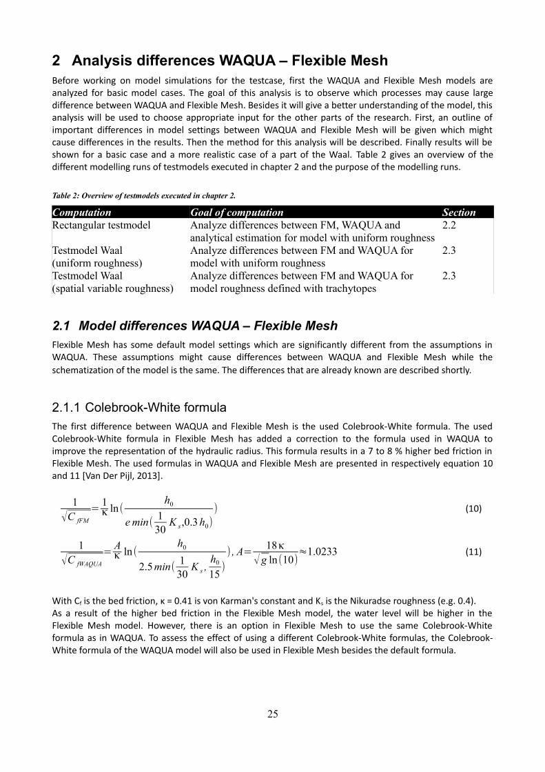
2.1.2 ConveyanceThe second difference is the default setting in Flexible Mesh to represent the bottom height within a gridcell. In WAQUA the bottom level within a grid cell is always constant, so the bed is schematized as ahorizontal tile. In Flexible Mesh the default setting enables to represent the bottom level in a cell by adiagonal tile between two bed level points. Especially in complex areas with relative large bed levelvariations, the representation in WAQUA may lead to inaccuracies in the water depth within a grid cell.Further, there is a height difference between the bed of two adjacent grid cells in the WAQUA modelbecause the bed level in the WAQUA model does not represent the real bed level at the bed level point.Therefore, there will be inaccuracies in the calculation of the equilibrium water depth. Because in FlexibleMesh the bed level may vary between two bed level points, the real bed level can be used at the bed levelpoints. (Figure 7) In Flexible Mesh there is also an option to disable the Conveyance2D setting and representthe bottom of a cell as a horizontal tile. This option will be used to assess the effect of representing the bedwithin a grid cell with a constant level or with a varying height.

2.1.3 Energy losses by weirsThe third difference is the modelling of energy losses by flow over weirs. In WAQUA the energy losses aredirectly added to the momentum equation as an opposing force by adding a term -gΔE/Δx to the right handside of the momentum equation [Rijkswaterstaat, 2012]. In Flexible Mesh a subgrid formulation is used forthe energy losses. Upstream of the weir there is calculated with conservation of energy and downstream ofthe weir there is calculated with conservation of momentum. Further, the formula for the calculation of theenergy height is not the same in WAQUA and Flexible Mesh. As there are many weirs in the Dutch rivers(e.g. groynes) the effect of weirs can be large. Therefore, model results with and without weirs will beobtained to assess the effect of weirs in WAQUA and Flexible Mesh.

2.1.4 Thin damsIn the schematization of a river many points where no water can flow are represented by thin dams. Anexample for a thin dam might be a structure (e.g. bridge pillars), which affects the flow in a river. Becausethe numerical method of WAQUA and Flexible Mesh is different, the effect of thin dams on the modelresults might be different. The effect of thin dams on the model results in Flexible Mesh and WAQUA will betested.

2.2 Rectangular testmodel

2.2.1 MethodFirst a small rectangular model is considered. This schematization is a very elementary schematization inwhich a rectangular grid of 2000x200 meter with grid cells of 40x40 meter is schematized. Therefore, thegrid contains 5 cells over the x-direction (m=6) and 50 cells over the y-direction (n=51). A constant discharge

26

Figure 7: Conveyance setting in WAQUA with horizontal tiles (left) and in Flexible Mesh with diagonal tiles (right).

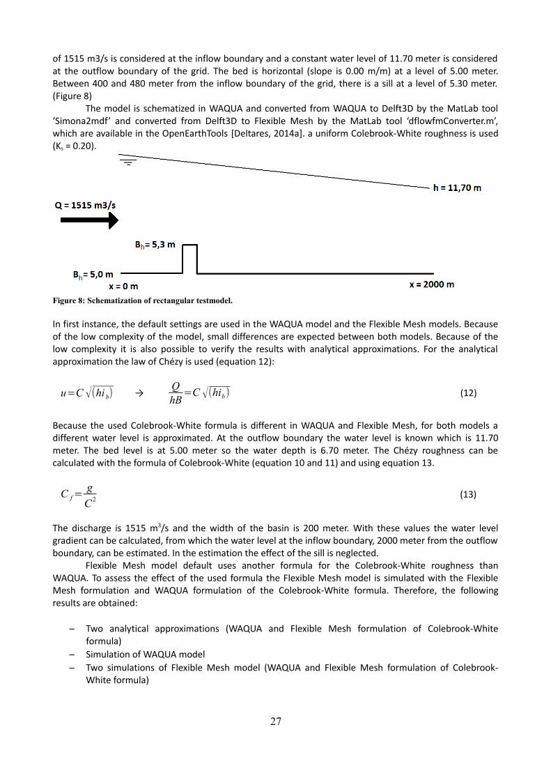
of 1515 m3/s is considered at the inflow boundary and a constant water level of 11.70 meter is consideredat the outflow boundary of the grid. The bed is horizontal (slope is 0.00 m/m) at a level of 5.00 meter.Between 400 and 480 meter from the inflow boundary of the grid, there is a sill at a level of 5.30 meter.(Figure 8)

The model is schematized in WAQUA and converted from WAQUA to Delft3D by the MatLab tool‘Simona2mdf’ and converted from Delft3D to Flexible Mesh by the MatLab tool ‘dflowfmConverter.m’,which are available in the OpenEarthTools [Deltares, 2014a]. a uniform Colebrook-White roughness is used(Ks = 0.20).

In first instance, the default settings are used in the WAQUA model and the Flexible Mesh models. Becauseof the low complexity of the model, small differences are expected between both models. Because of thelow complexity it is also possible to verify the results with analytical approximations. For the analyticalapproximation the law of Chézy is used (equation 12):

u=C √(hi b) → QhB

=C √(hib) (12)

Because the used Colebrook-White formula is different in WAQUA and Flexible Mesh, for both models adifferent water level is approximated. At the outflow boundary the water level is known which is 11.70meter. The bed level is at 5.00 meter so the water depth is 6.70 meter. The Chézy roughness can becalculated with the formula of Colebrook-White (equation 10 and 11) and using equation 13.

C f=g

C2 (13)

The discharge is 1515 m3/s and the width of the basin is 200 meter. With these values the water levelgradient can be calculated, from which the water level at the inflow boundary, 2000 meter from the outflowboundary, can be estimated. In the estimation the effect of the sill is neglected.

Flexible Mesh model default uses another formula for the Colebrook-White roughness thanWAQUA. To assess the effect of the used formula the Flexible Mesh model is simulated with the FlexibleMesh formulation and WAQUA formulation of the Colebrook-White formula. Therefore, the followingresults are obtained:

– Two analytical approximations (WAQUA and Flexible Mesh formulation of Colebrook-Whiteformula)

– Simulation of WAQUA model– Two simulations of Flexible Mesh model (WAQUA and Flexible Mesh formulation of Colebrook-

White formula)

27

Figure 8: Schematization of rectangular testmodel.

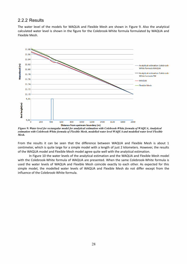
2.2.2 ResultsThe water level of the models for WAQUA and Flexible Mesh are shown in Figure 9. Also the analyticalcalculated water level is shown in the figure for the Colebrook-White formula formulated by WAQUA andFlexible Mesh.

From the results it can be seen that the difference between WAQUA and Flexible Mesh is about 1centimeter, which is quite large for a simple model with a length of just 2 kilometers. However, the resultsof the WAQUA model and Flexible Mesh model agree quite well with the analytical estimation.

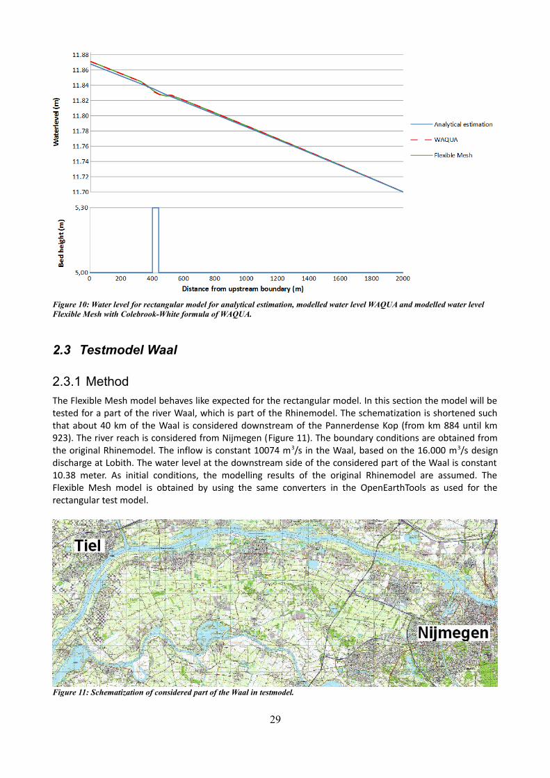
In Figure 10 the water levels of the analytical estimation and the WAQUA and Flexible Mesh modelwith the Colebrook-White formula of WAQUA are presented. When the same Colebrook-White formula isused the water levels of WAQUA and Flexible Mesh coincide exactly to each other. As expected for thissimple model, the modelled water levels of WAQUA and Flexible Mesh do not differ except from theinfluence of the Colebrook-White formula.

28

Figure 9: Water level for rectangular model for analytical estimation with Colebrook-White formula of WAQUA, Analytical estimation with Colebrook-White formula of Flexible Mesh, modelled water level WAQUA and modelled water level Flexible Mesh.

2.3 Testmodel Waal

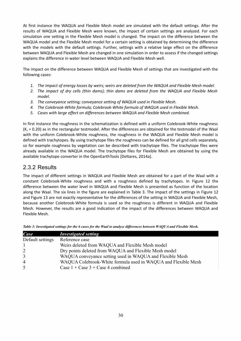
2.3.1 MethodThe Flexible Mesh model behaves like expected for the rectangular model. In this section the model will betested for a part of the river Waal, which is part of the Rhinemodel. The schematization is shortened suchthat about 40 km of the Waal is considered downstream of the Pannerdense Kop (from km 884 until km923). The river reach is considered from Nijmegen (Figure 11). The boundary conditions are obtained fromthe original Rhinemodel. The inflow is constant 10074 m3/s in the Waal, based on the 16.000 m3/s designdischarge at Lobith. The water level at the downstream side of the considered part of the Waal is constant10.38 meter. As initial conditions, the modelling results of the original Rhinemodel are assumed. TheFlexible Mesh model is obtained by using the same converters in the OpenEarthTools as used for therectangular test model.

29

Figure 11: Schematization of considered part of the Waal in testmodel.

Figure 10: Water level for rectangular model for analytical estimation, modelled water level WAQUA and modelled water level Flexible Mesh with Colebrook-White formula of WAQUA.

At first instance the WAQUA and Flexible Mesh model are simulated with the default settings. After theresults of WAQUA and Flexible Mesh were known, the impact of certain settings are analyzed. For eachsimulation one setting in the Flexible Mesh model is changed. The impact on the difference between theWAQUA model and the Flexible Mesh model for a certain setting is obtained by determining the differencewith the models with the default settings. Further, settings with a relative large effect on the differencebetween WAQUA and Flexible Mesh are changed in one simulation in order to assess if the changed settingsexplains the difference in water level between WAQUA and Flexible Mesh well.

The impact on the difference between WAQUA and Flexible Mesh of settings that are investigated with thefollowing cases:

1. The impact of energy losses by weirs; weirs are deleted from the WAQUA and Flexible Mesh model.2. The impact of dry cells (thin dams); thin dams are deleted from the WAQUA and Flexible Mesh

model.3. The conveyance setting; conveyance setting of WAQUA used in Flexible Mesh.4. The Colebrook-White formula; Colebrook-White formula of WAQUA used in Flexible Mesh.5. Cases with large effect on differences between WAQUA and Flexible Mesh combined.

In first instance the roughness in the schematization is defined with a uniform Colebrook-White roughness(Ks = 0.20) as in the rectangular testmodel. After the differences are obtained for the testmodel of the Waalwith the uniform Colebrook-White roughness, the roughness in the WAQUA and Flexible Mesh model isdefined with trachytopes. By using trachytope files the roughness can be defined for all grid cells separately,so for example roughness by vegetation can be described with trachytope files. The trachytope files werealready available in the WAQUA model. The trachytope files for Flexible Mesh are obtained by using theavailable trachytope converter in the OpenEarthTools [Deltares, 2014a].

2.3.2 ResultsThe impact of different settings in WAQUA and Flexible Mesh are obtained for a part of the Waal with aconstant Colebrook-White roughness and with a roughness defined by trachytopes. In Figure 12 thedifference between the water level in WAQUA and Flexible Mesh is presented as function of the locationalong the Waal. The six lines in the figure are explained in Table 3. The impact of the settings in Figure 12and Figure 13 are not exactly representative for the differences of the setting in WAQUA and Flexible Mesh,because another Colebrook-White formula is used so the roughness is different in WAQUA and FlexibleMesh. However, the results are a good indication of the impact of the differences between WAQUA andFlexible Mesh.

Table 3: Investigated settings for the 6 cases for the Waal to analyze differences between WAQUA and Flexible Mesh.

Case Investigated settingDefault settings Reference case1 Weirs deleted from WAQUA and Flexible Mesh model2 Dry points deleted from WAQUA and Flexible Mesh model3 WAQUA conveyance setting used in WAQUA and Flexible Mesh4 WAQUA Colebrook-White formula used in WAQUA and Flexible Mesh5 Case 1 + Case 3 + Case 4 combined

30

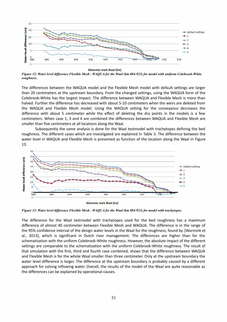
The differences between the WAQUA model and the Flexible Mesh model with default settings are largerthan 20 centimeters at the upstream boundary. From the changed settings, using the WAQUA form of theColebrook-White has the largest impact. The difference between WAQUA and Flexible Mesh is more thanhalved. Further the difference has decreased with about 5-10 centimeters when the weirs are deleted fromthe WAQUA and Flexible Mesh model. Using the WAQUA setting for the conveyance decreases thedifference with about 5 centimeter while the effect of deleting the dry points in the models is a fewcentimeters. When case 1, 3 and 4 are combined the differences between WAQUA and Flexible Mesh aresmaller than five centimeters at all locations along the Waal.

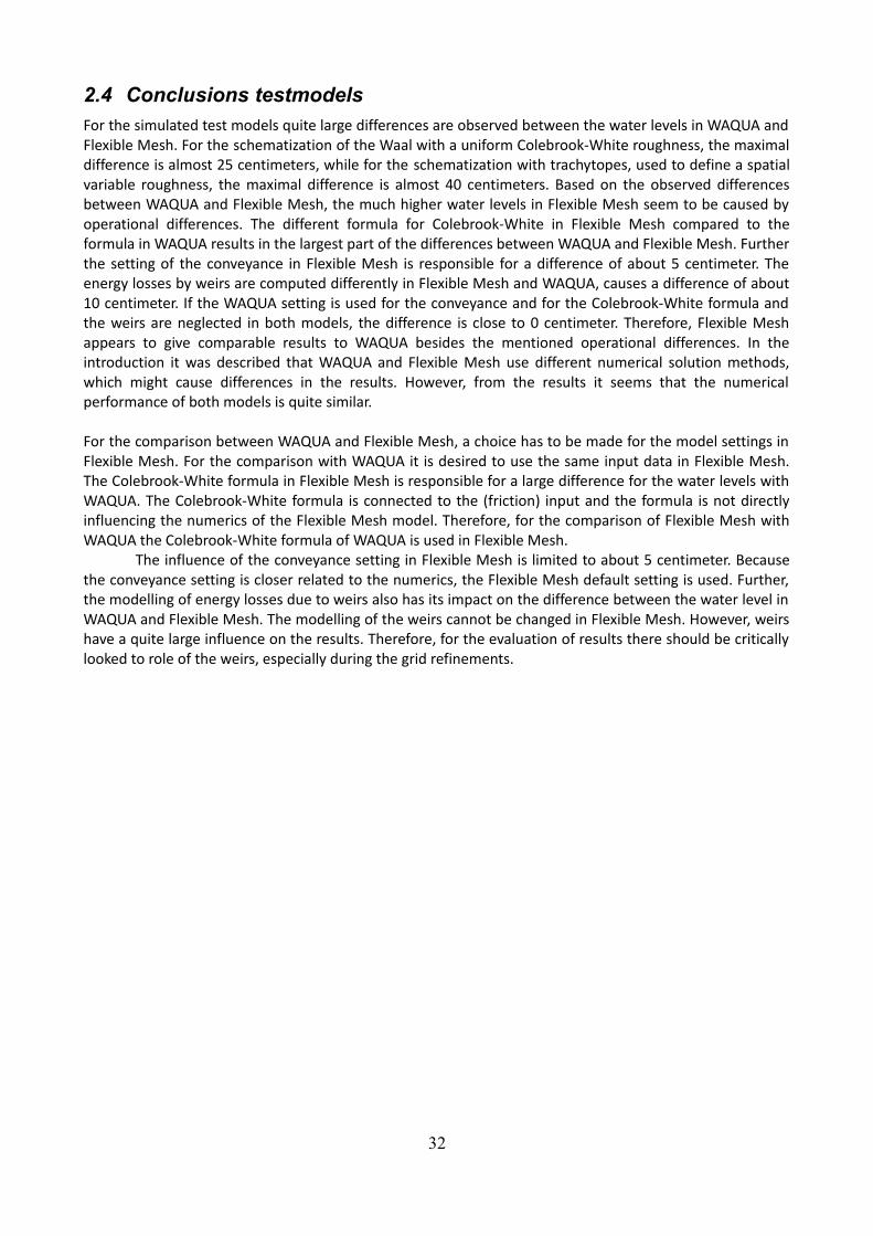
Subsequently the same analysis is done for the Waal testmodel with trachytopes defining the bedroughness. The different cases which are investigated are explained in Table 3. The difference between thewater level in WAQUA and Flexible Mesh is presented as function of the location along the Waal in Figure13.

The difference for the Waal testmodel with trachytopes used for the bed roughness has a maximumdifference of almost 40 centimeter between Flexible Mesh and WAQUA. The difference is in the range ofthe 95% confidence interval of the design water levels in the Waal for the roughness, found by [Warmink etal., 2013], which is significant in Dutch river management. The differences are higher than for theschematization with the uniform Colebrook-White roughness. However, the absolute impact of the differentsettings are comparable to the schematization with the uniform Colebrook-White roughness. The result ofthat simulation with the first, third and fourth case combined, shows that the difference between WAQUAand Flexible Mesh is for the whole Waal smaller than three centimeter. Only at the upstream boundary thewater level difference is larger. The difference at the upstream boundary is probably caused by a differentapproach for solving inflowing water. Overall, the results of the model of the Waal are quite reasonable asthe differences can be explained by operational causes.

31

Figure 13: Water level difference Flexible Mesh - WAQUA for the Waal (km 884-923) for model with trachytopes.

Figure 12: Water level difference Flexible Mesh - WAQUA for the Waal (km 884-923) for model with uniform Colebrook-White roughness.

2.4 Conclusions testmodelsFor the simulated test models quite large differences are observed between the water levels in WAQUA andFlexible Mesh. For the schematization of the Waal with a uniform Colebrook-White roughness, the maximaldifference is almost 25 centimeters, while for the schematization with trachytopes, used to define a spatialvariable roughness, the maximal difference is almost 40 centimeters. Based on the observed differencesbetween WAQUA and Flexible Mesh, the much higher water levels in Flexible Mesh seem to be caused byoperational differences. The different formula for Colebrook-White in Flexible Mesh compared to theformula in WAQUA results in the largest part of the differences between WAQUA and Flexible Mesh. Furtherthe setting of the conveyance in Flexible Mesh is responsible for a difference of about 5 centimeter. Theenergy losses by weirs are computed differently in Flexible Mesh and WAQUA, causes a difference of about10 centimeter. If the WAQUA setting is used for the conveyance and for the Colebrook-White formula andthe weirs are neglected in both models, the difference is close to 0 centimeter. Therefore, Flexible Meshappears to give comparable results to WAQUA besides the mentioned operational differences. In theintroduction it was described that WAQUA and Flexible Mesh use different numerical solution methods,which might cause differences in the results. However, from the results it seems that the numericalperformance of both models is quite similar.

For the comparison between WAQUA and Flexible Mesh, a choice has to be made for the model settings inFlexible Mesh. For the comparison with WAQUA it is desired to use the same input data in Flexible Mesh.The Colebrook-White formula in Flexible Mesh is responsible for a large difference for the water levels withWAQUA. The Colebrook-White formula is connected to the (friction) input and the formula is not directlyinfluencing the numerics of the Flexible Mesh model. Therefore, for the comparison of Flexible Mesh withWAQUA the Colebrook-White formula of WAQUA is used in Flexible Mesh.

The influence of the conveyance setting in Flexible Mesh is limited to about 5 centimeter. Becausethe conveyance setting is closer related to the numerics, the Flexible Mesh default setting is used. Further,the modelling of energy losses due to weirs also has its impact on the difference between the water level inWAQUA and Flexible Mesh. The modelling of the weirs cannot be changed in Flexible Mesh. However, weirshave a quite large influence on the results. Therefore, for the evaluation of results there should be criticallylooked to role of the weirs, especially during the grid refinements.

32

3 Methodology of comparison and grid refinementIn the previous chapter the differences between WAQUA and Flexible Mesh are analyzed. From thesimulated testcases a better understanding is obtained from the Flexible Mesh model. The following step isthe comparison between modelling results of WAQUA and Flexible Mesh for the case study (researchquestion 2). For the comparison a calibrated WAQUA model will be used which schematizes a real situation.The comparison is done for the Waal with and without side channel at Afferden and Deest. The second stepis the application of grid refinement to the side channel at Afferden and Deest (research question 3). In thischapter, the research method for both steps will be described.

3.1 Comparison Flexible Mesh – WAQUAThe comparison between Flexible Mesh and WAQUA is done for the Waal with special focus on theAfferdense and Deestse Waarden. For the Waal without side channel, a Rhinemodel in WAQUA is availablewhich is calibrated based on the high water in 1995. There are also water level measurements available for1995. For the Waal with side channel, a Rhinemodel is available in which several measures areimplemented, including the side channel at Afferden and Deest. Both cases will be described in this section.

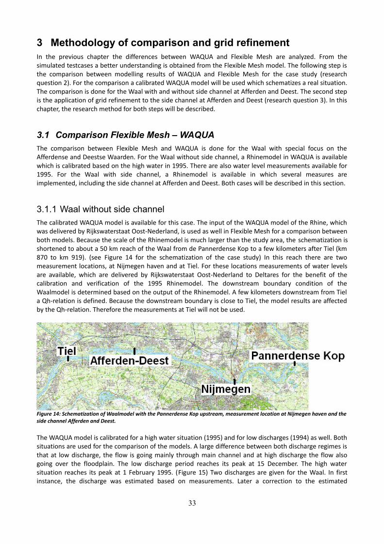
3.1.1 Waal without side channelThe calibrated WAQUA model is available for this case. The input of the WAQUA model of the Rhine, whichwas delivered by Rijkswaterstaat Oost-Nederland, is used as well in Flexible Mesh for a comparison betweenboth models. Because the scale of the Rhinemodel is much larger than the study area, the schematization isshortened to about a 50 km reach of the Waal from de Pannerdense Kop to a few kilometers after Tiel (km870 to km 919). (see Figure 14 for the schematization of the case study) In this reach there are twomeasurement locations, at Nijmegen haven and at Tiel. For these locations measurements of water levelsare available, which are delivered by Rijkswaterstaat Oost-Nederland to Deltares for the benefit of thecalibration and verification of the 1995 Rhinemodel. The downstream boundary condition of theWaalmodel is determined based on the output of the Rhinemodel. A few kilometers downstream from Tiela Qh-relation is defined. Because the downstream boundary is close to Tiel, the model results are affectedby the Qh-relation. Therefore the measurements at Tiel will not be used.

The WAQUA model is calibrated for a high water situation (1995) and for low discharges (1994) as well. Bothsituations are used for the comparison of the models. A large difference between both discharge regimes isthat at low discharge, the flow is going mainly through main channel and at high discharge the flow alsogoing over the floodplain. The low discharge period reaches its peak at 15 December. The high watersituation reaches its peak at 1 February 1995. (Figure 15) Two discharges are given for the Waal. In firstinstance, the discharge was estimated based on measurements. Later a correction to the estimated

33

Figure 14: Schematization of Waalmodel with the Pannerdense Kop upstream, measurement location at Nijmegen haven and theside channel Afferden and Deest.

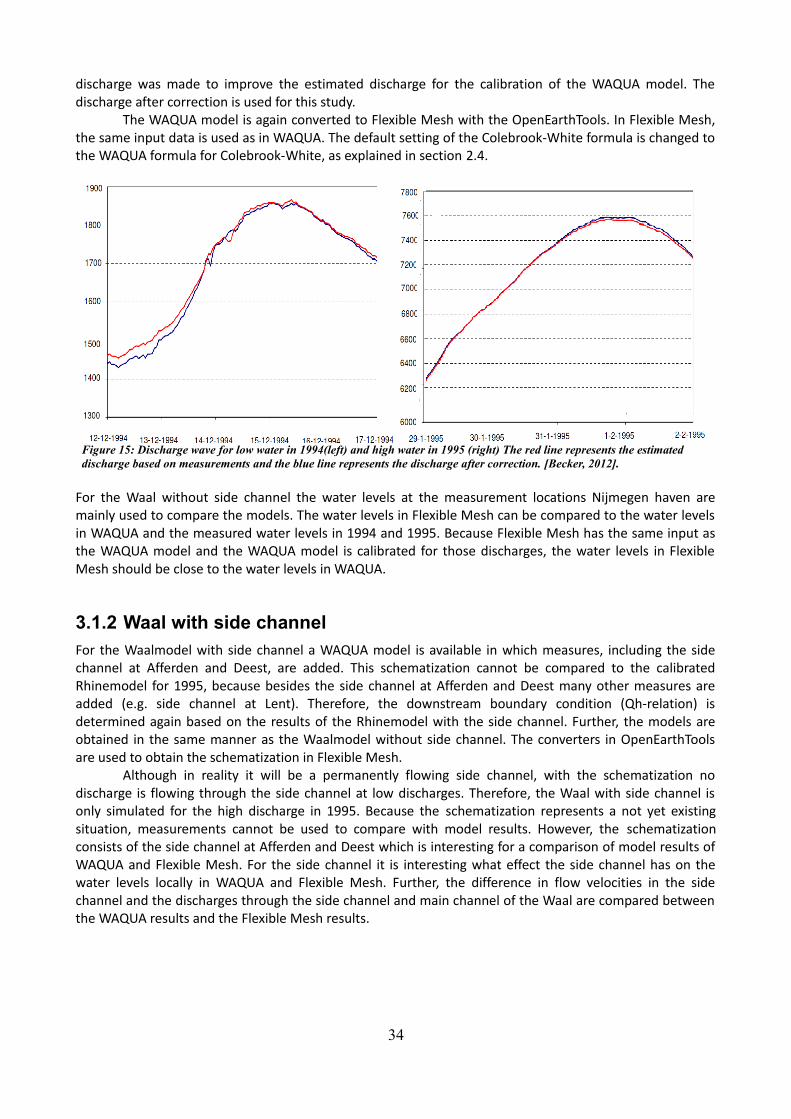
discharge was made to improve the estimated discharge for the calibration of the WAQUA model. Thedischarge after correction is used for this study.

The WAQUA model is again converted to Flexible Mesh with the OpenEarthTools. In Flexible Mesh,the same input data is used as in WAQUA. The default setting of the Colebrook-White formula is changed tothe WAQUA formula for Colebrook-White, as explained in section 2.4.

For the Waal without side channel the water levels at the measurement locations Nijmegen haven aremainly used to compare the models. The water levels in Flexible Mesh can be compared to the water levelsin WAQUA and the measured water levels in 1994 and 1995. Because Flexible Mesh has the same input asthe WAQUA model and the WAQUA model is calibrated for those discharges, the water levels in FlexibleMesh should be close to the water levels in WAQUA.

3.1.2 Waal with side channelFor the Waalmodel with side channel a WAQUA model is available in which measures, including the sidechannel at Afferden and Deest, are added. This schematization cannot be compared to the calibratedRhinemodel for 1995, because besides the side channel at Afferden and Deest many other measures areadded (e.g. side channel at Lent). Therefore, the downstream boundary condition (Qh-relation) isdetermined again based on the results of the Rhinemodel with the side channel. Further, the models areobtained in the same manner as the Waalmodel without side channel. The converters in OpenEarthToolsare used to obtain the schematization in Flexible Mesh.

Although in reality it will be a permanently flowing side channel, with the schematization nodischarge is flowing through the side channel at low discharges. Therefore, the Waal with side channel isonly simulated for the high discharge in 1995. Because the schematization represents a not yet existingsituation, measurements cannot be used to compare with model results. However, the schematizationconsists of the side channel at Afferden and Deest which is interesting for a comparison of model results ofWAQUA and Flexible Mesh. For the side channel it is interesting what effect the side channel has on thewater levels locally in WAQUA and Flexible Mesh. Further, the difference in flow velocities in the sidechannel and the discharges through the side channel and main channel of the Waal are compared betweenthe WAQUA results and the Flexible Mesh results.

34

Figure 15: Discharge wave for low water in 1994(left) and high water in 1995 (right) The red line represents the estimated discharge based on measurements and the blue line represents the discharge after correction. [Becker, 2012].

3.2 Grid refinementLocal grid refinement is applied to the case project Afferden-Deest to assess the impact on the results of theFlexible Mesh model. The grid refinement is applied to the main channel of the Waal next to the sidechannel at Afferden and Deest and to the side channel at Afferden and Deest itself. First, the setup of themodel for the grid refinement is explained.

3.2.1 Model setupFor the study of the local grid refinement as reference situation the same schematization of the Waal withside channel is used as for the comparison of WAQUA and Flexible Mesh. The high discharge of 1995 isconsidered for the model. The use of the trachytope files to define the roughness is not yet supported forthe unstructured grid in Flexible Mesh. However, to assess the effect of local grid refinement the samemodel settings are needed for different simulations. Therefore the output of the roughness from theFlexible Mesh model with the original schematization is used as input for the simulations in the study oflocal grid refinements. The Colebrook-White values for all network links at the peak of the discharge waveare exported. The netlinks in the file are written to x- and y-coordinates such that the file can be used asinput file. In the schematization all default settings of Flexible Mesh are used. So in this schematization thedefault Colebrook-White formula for Flexible Mesh is used.

For the reference schematization the input data is projected on the network of Flexible Mesh. Whenthe grid is adapted the input data is not any more defined on the network. Therefore, when the grid isrefined the input data (roughness and bathymetry) is newly projected to the adapted part of the network.The data is interpolated to the network links of the grid.

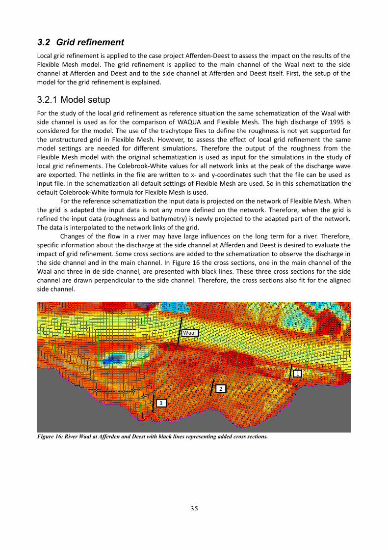
Changes of the flow in a river may have large influences on the long term for a river. Therefore,specific information about the discharge at the side channel at Afferden and Deest is desired to evaluate theimpact of grid refinement. Some cross sections are added to the schematization to observe the discharge inthe side channel and in the main channel. In Figure 16 the cross sections, one in the main channel of theWaal and three in de side channel, are presented with black lines. These three cross sections for the sidechannel are drawn perpendicular to the side channel. Therefore, the cross sections also fit for the alignedside channel.

35

Figure 16: River Waal at Afferden and Deest with black lines representing added cross sections.

3.2.2 Grid refinement main channelFirst, the grid refinement is applied to the main channel of the Waal over the length of 4 kilometer next tothe side channel at Afferden and Deest. The refinement of the Waal channel is used as reference situationfor the refinement of the side channel. The variations between adjacent grid cells are much larger in theside channel than in the main channel of the Waal. Therefore, the expectation is that the WAQUA grid isquite accurate for the main channel of the Waal, but is inaccurate for the side channel at Afferden andDeest. The refinement of the Waal channel is used to check if the effect of refining the grid of the sidechannel is indeed larger than refining the grid of the Waal channel.

The grid of the main channel of the Waal is refined over the width, so the length of the cellsremains the same but the number of cells over the width of the Waal channel increases. In Flexible Mesh,this grid refinement is executed automatically by defining the grid to be refined with a polygon. The cells arerefined by using the Casulli-type mesh refinement. After the automatical refinement the quality of the gridis monitored and improved where needed. Particularly at the boundary of the refinement, where thetransition from the original grid to the refined grid is, the mesh quality might have some trouble with theorthogonality. The model is simulated with the WAQUA grid and with the grid resolution two, four and eighttimes increased compared to the reference situation. Because the impact of the grid refinement in the Waalchannel is expected to be limited, the model results are probably not much affected by higher gridresolutions.

3.2.3 Grid refinement side channel (not aligned)The grid refinement for the side channel is executed with help of the bathymetry data. The refined part ofthe grid includes the parts of the side channel in which the variation in bed level between adjacent grid cellsis relative large. The refinement is extended from the inlet to the outlet channel of the side channel. A withthe flow direction aligned grid is assumed to be computational more efficient. Therefore, the gridrefinement in the side channel is applied with an aligned and not aligned grid refinement.

The grid refinement is, just as for the refinement of the main channel of the Waal, executed overthe width of the side channel, so the length of the grid cells remains the same. The grid refinement withoutalignment is executed by defining a polygon and applying the Casulli-type refinement on the originalWAQUA grid which refines the grid within the polygon two times.

3.2.4 Grid refinement side channel (aligned)Last, the original grid in the side channel is refined with aligning the grid cells to the flow direction

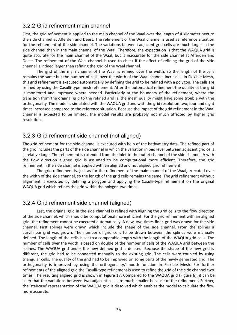
of the side channel, which should be computational more efficient. For the grid refinement with an alignedgrid, the refinement cannot be executed automatically. A new, two times finer, grid was drawn for the sidechannel. First splines were drawn which include the shape of the side channel. From the splines acurvilinear grid was grown. The number of grid cells to be drawn between the splines were manuallydefined. The length of the cells is set to a comparable length with the length of the WAQUA grid cells. Thenumber of cells over the width is based on double of the number of cells of the WAQUA grid between thesplines. The WAQUA grid under the new defined grid is deleted. Because the shape of the new grid isdifferent, the grid had to be connected manually to the existing grid. The cells were coupled by usingtriangular cells. The quality of the grid had to be improved on some parts of the newly generated grid. Theorthogonality is improved by using the orthogonality/smooth function in Flexible Mesh. For furtherrefinements of the aligned grid the Casulli-type refinement is used to refine the grid of the side channel twotimes. The resulting aligned grid is shown in Figure 17. Compared to the WAQUA grid (Figure 6), it can beseen that the variations between two adjacent cells are much smaller because of the refinement. Further,the 'staircase' representation of the WAQUA grid is dissolved which enables the model to calculate the flowmore accurate.

36

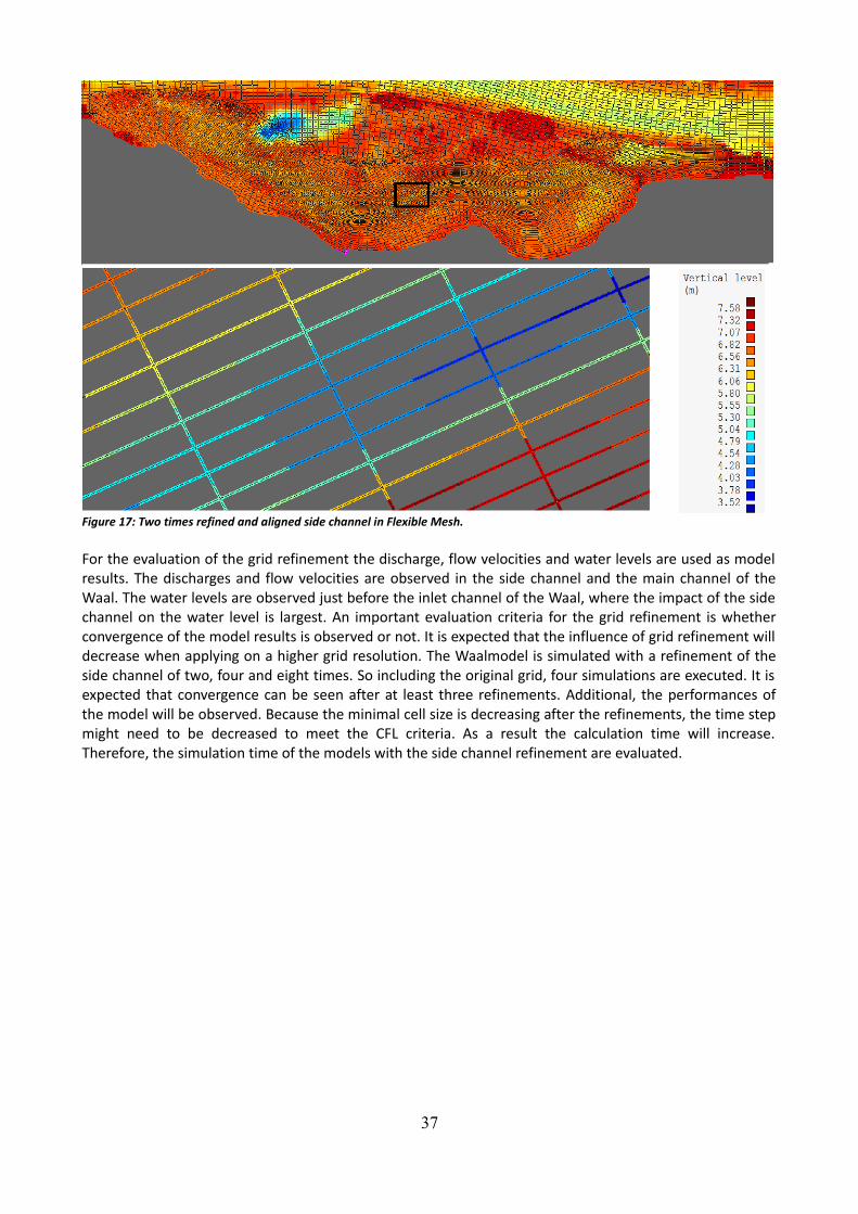
For the evaluation of the grid refinement the discharge, flow velocities and water levels are used as modelresults. The discharges and flow velocities are observed in the side channel and the main channel of theWaal. The water levels are observed just before the inlet channel of the Waal, where the impact of the sidechannel on the water level is largest. An important evaluation criteria for the grid refinement is whetherconvergence of the model results is observed or not. It is expected that the influence of grid refinement willdecrease when applying on a higher grid resolution. The Waalmodel is simulated with a refinement of theside channel of two, four and eight times. So including the original grid, four simulations are executed. It isexpected that convergence can be seen after at least three refinements. Additional, the performances ofthe model will be observed. Because the minimal cell size is decreasing after the refinements, the time stepmight need to be decreased to meet the CFL criteria. As a result the calculation time will increase.Therefore, the simulation time of the models with the side channel refinement are evaluated.

37

Figure 17: Two times refined and aligned side channel in Flexible Mesh.

4 ResultsIn this chapter the results of the research are presented. First the results of the comparison betweenWAQUA and Flexible Mesh will be described (research question 2). The comparison consists of aschematization without side channel for which measurements are available and a schematization with sidechannel. Secondly the results of the local grid refinement at Afferden and Deest will be presented (researchquestion 3). The local grid refinement is divided in a refinement of the main channel of the Waal and arefinement of the side channel. Table 4 gives an overview of the different modelling runs executed inchapter 4 and the purpose of the modelling runs.

Table 4: Overview of testmodels executed in chapter 2.

Computation Goal of computation SectionWaalmodel without side channel

Compare model results of FM with calibrated WAQUA model and measurements for the Waal

4.1.1

Waalmodel with side channel Compare model results of FM with WAQUA for the casestudy Afferden and Deest

4.1.2

Local grid refinement in main channel of Waal

Assess effect of local grid refinement in main channel of Waal as reference case

4.2.1

Local grid refinement in side channel without alignment

Assess effect of local grid refinement in side channel without aligning the grid to the flow direction

4.2.2

Local grid refinement in side cannel with alignment

Assess effect of local grid refinement in side channel with aligned grid to flow direction

4.2.3

4.1 Comparison Flexible Mesh – WAQUAThis section describes the results for the comparison between Flexible Mesh and WAQUA for the Waal withand without side channel. As described in Chapter 3, for these simulations the Colebrook-White formula ofWAQUA is used in Flexible Mesh. Further, the default settings of Flexible Mesh are used.

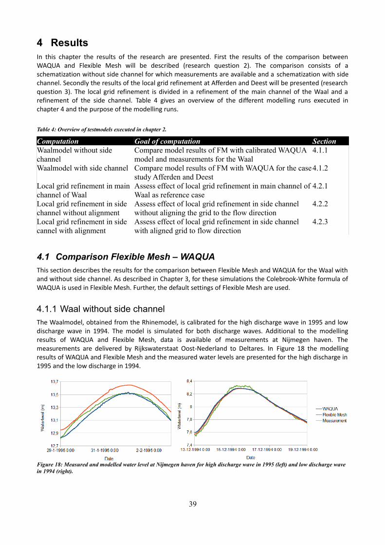
4.1.1 Waal without side channelThe Waalmodel, obtained from the Rhinemodel, is calibrated for the high discharge wave in 1995 and lowdischarge wave in 1994. The model is simulated for both discharge waves. Additional to the modellingresults of WAQUA and Flexible Mesh, data is available of measurements at Nijmegen haven. Themeasurements are delivered by Rijkswaterstaat Oost-Nederland to Deltares. In Figure 18 the modellingresults of WAQUA and Flexible Mesh and the measured water levels are presented for the high discharge in1995 and the low discharge in 1994.

39

Figure 18: Measured and modelled water level at Nijmegen haven for high discharge wave in 1995 (left) and low discharge wave in 1994 (right).

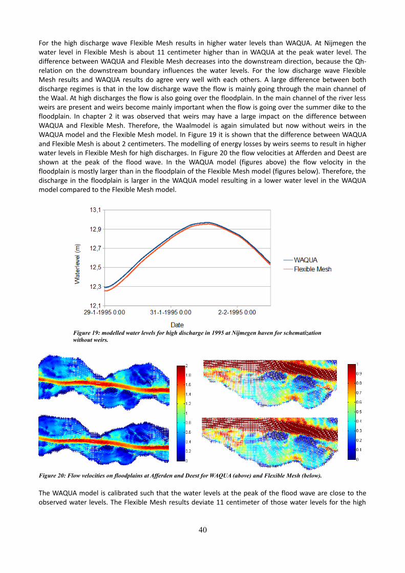
For the high discharge wave Flexible Mesh results in higher water levels than WAQUA. At Nijmegen thewater level in Flexible Mesh is about 11 centimeter higher than in WAQUA at the peak water level. Thedifference between WAQUA and Flexible Mesh decreases into the downstream direction, because the Qh-relation on the downstream boundary influences the water levels. For the low discharge wave FlexibleMesh results and WAQUA results do agree very well with each others. A large difference between bothdischarge regimes is that in the low discharge wave the flow is mainly going through the main channel ofthe Waal. At high discharges the flow is also going over the floodplain. In the main channel of the river lessweirs are present and weirs become mainly important when the flow is going over the summer dike to thefloodplain. In chapter 2 it was observed that weirs may have a large impact on the difference betweenWAQUA and Flexible Mesh. Therefore, the Waalmodel is again simulated but now without weirs in theWAQUA model and the Flexible Mesh model. In Figure 19 it is shown that the difference between WAQUAand Flexible Mesh is about 2 centimeters. The modelling of energy losses by weirs seems to result in higherwater levels in Flexible Mesh for high discharges. In Figure 20 the flow velocities at Afferden and Deest areshown at the peak of the flood wave. In the WAQUA model (figures above) the flow velocity in thefloodplain is mostly larger than in the floodplain of the Flexible Mesh model (figures below). Therefore, thedischarge in the floodplain is larger in the WAQUA model resulting in a lower water level in the WAQUAmodel compared to the Flexible Mesh model.

The WAQUA model is calibrated such that the water levels at the peak of the flood wave are close to theobserved water levels. The Flexible Mesh results deviate 11 centimeter of those water levels for the high

40

Figure 19: modelled water levels for high discharge in 1995 at Nijmegen haven for schematization without weirs.

Figure 20: Flow velocities on floodplains at Afferden and Deest for WAQUA (above) and Flexible Mesh (below).

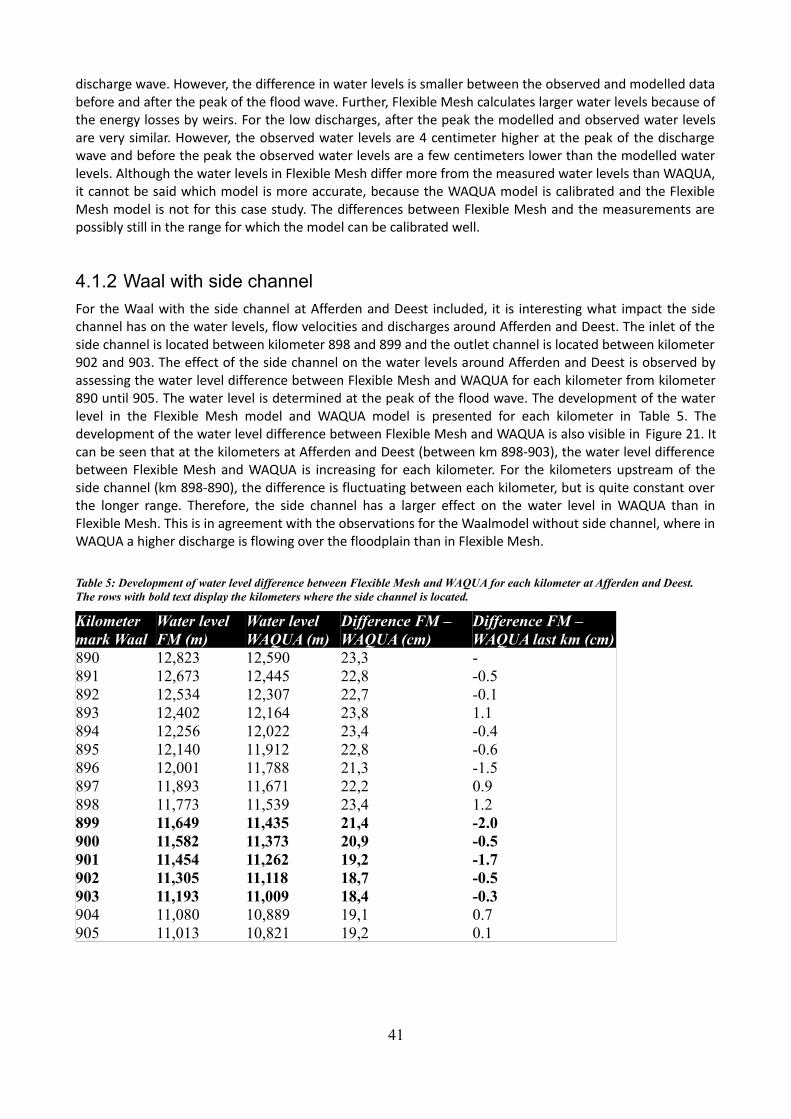
discharge wave. However, the difference in water levels is smaller between the observed and modelled databefore and after the peak of the flood wave. Further, Flexible Mesh calculates larger water levels because ofthe energy losses by weirs. For the low discharges, after the peak the modelled and observed water levelsare very similar. However, the observed water levels are 4 centimeter higher at the peak of the dischargewave and before the peak the observed water levels are a few centimeters lower than the modelled waterlevels. Although the water levels in Flexible Mesh differ more from the measured water levels than WAQUA,it cannot be said which model is more accurate, because the WAQUA model is calibrated and the FlexibleMesh model is not for this case study. The differences between Flexible Mesh and the measurements arepossibly still in the range for which the model can be calibrated well.

4.1.2 Waal with side channelFor the Waal with the side channel at Afferden and Deest included, it is interesting what impact the sidechannel has on the water levels, flow velocities and discharges around Afferden and Deest. The inlet of theside channel is located between kilometer 898 and 899 and the outlet channel is located between kilometer902 and 903. The effect of the side channel on the water levels around Afferden and Deest is observed byassessing the water level difference between Flexible Mesh and WAQUA for each kilometer from kilometer890 until 905. The water level is determined at the peak of the flood wave. The development of the waterlevel in the Flexible Mesh model and WAQUA model is presented for each kilometer in Table 5. Thedevelopment of the water level difference between Flexible Mesh and WAQUA is also visible in Figure 21. Itcan be seen that at the kilometers at Afferden and Deest (between km 898-903), the water level differencebetween Flexible Mesh and WAQUA is increasing for each kilometer. For the kilometers upstream of theside channel (km 898-890), the difference is fluctuating between each kilometer, but is quite constant overthe longer range. Therefore, the side channel has a larger effect on the water level in WAQUA than inFlexible Mesh. This is in agreement with the observations for the Waalmodel without side channel, where inWAQUA a higher discharge is flowing over the floodplain than in Flexible Mesh.

Table 5: Development of water level difference between Flexible Mesh and WAQUA for each kilometer at Afferden and Deest. The rows with bold text display the kilometers where the side channel is located.

Kilometer mark Waal

Water level FM (m)

Water level WAQUA (m)

Difference FM – WAQUA (cm)

Difference FM – WAQUA last km (cm)

890 12,823 12,590 23,3 -891 12,673 12,445 22,8 -0.5892 12,534 12,307 22,7 -0.1893 12,402 12,164 23,8 1.1894 12,256 12,022 23,4 -0.4895 12,140 11,912 22,8 -0.6896 12,001 11,788 21,3 -1.5897 11,893 11,671 22,2 0.9898 11,773 11,539 23,4 1.2899 11,649 11,435 21,4 -2.0900 11,582 11,373 20,9 -0.5901 11,454 11,262 19,2 -1.7902 11,305 11,118 18,7 -0.5903 11,193 11,009 18,4 -0.3904 11,080 10,889 19,1 0.7905 11,013 10,821 19,2 0.1

41

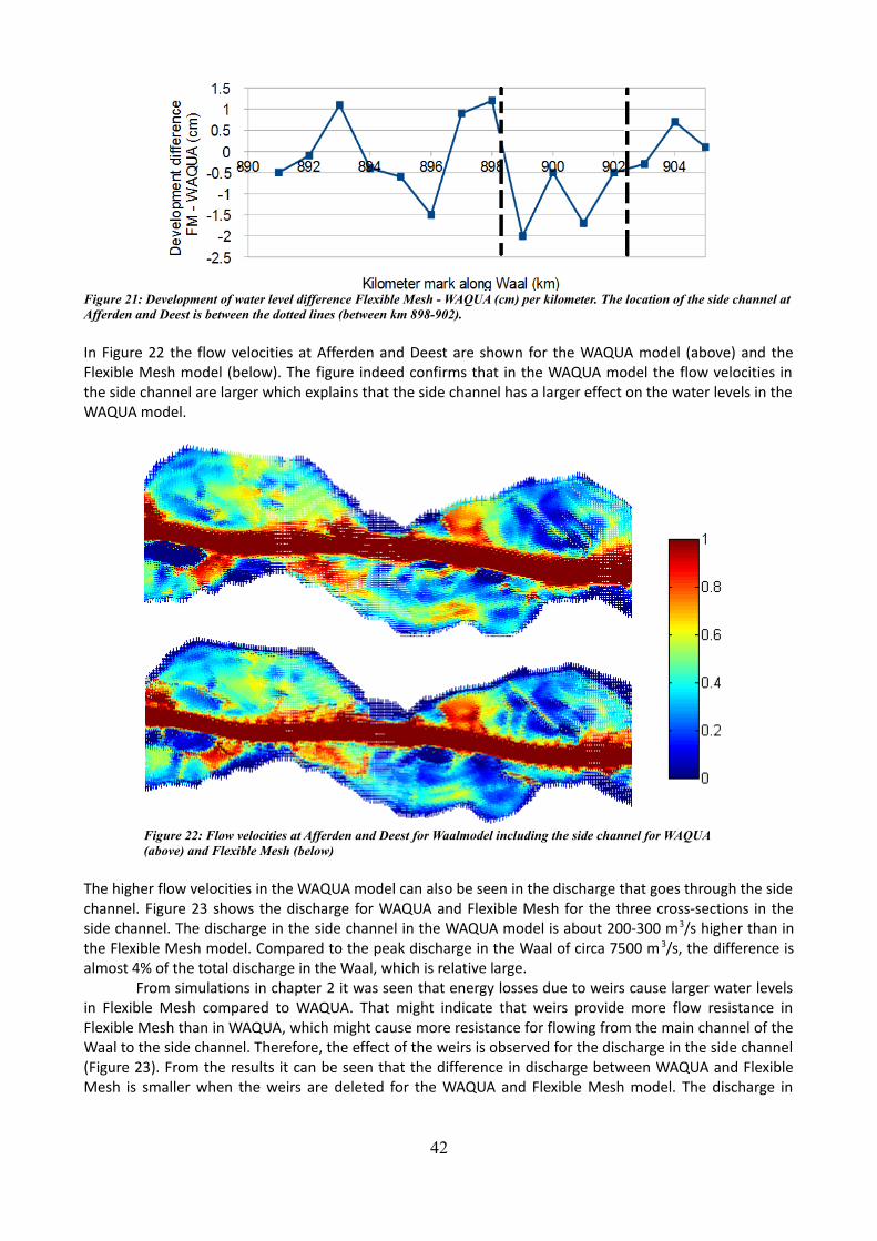
In Figure 22 the flow velocities at Afferden and Deest are shown for the WAQUA model (above) and theFlexible Mesh model (below). The figure indeed confirms that in the WAQUA model the flow velocities inthe side channel are larger which explains that the side channel has a larger effect on the water levels in theWAQUA model.

The higher flow velocities in the WAQUA model can also be seen in the discharge that goes through the sidechannel. Figure 23 shows the discharge for WAQUA and Flexible Mesh for the three cross-sections in theside channel. The discharge in the side channel in the WAQUA model is about 200-300 m3/s higher than inthe Flexible Mesh model. Compared to the peak discharge in the Waal of circa 7500 m 3/s, the difference isalmost 4% of the total discharge in the Waal, which is relative large.

From simulations in chapter 2 it was seen that energy losses due to weirs cause larger water levelsin Flexible Mesh compared to WAQUA. That might indicate that weirs provide more flow resistance inFlexible Mesh than in WAQUA, which might cause more resistance for flowing from the main channel of theWaal to the side channel. Therefore, the effect of the weirs is observed for the discharge in the side channel(Figure 23). From the results it can be seen that the difference in discharge between WAQUA and FlexibleMesh is smaller when the weirs are deleted for the WAQUA and Flexible Mesh model. The discharge in

42

Figure 22: Flow velocities at Afferden and Deest for Waalmodel including the side channel for WAQUA (above) and Flexible Mesh (below)

Figure 21: Development of water level difference Flexible Mesh - WAQUA (cm) per kilometer. The location of the side channel atAfferden and Deest is between the dotted lines (between km 898-902).

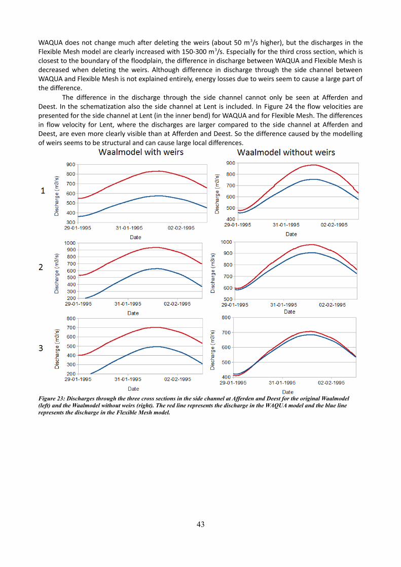
WAQUA does not change much after deleting the weirs (about 50 m3/s higher), but the discharges in theFlexible Mesh model are clearly increased with 150-300 m3/s. Especially for the third cross section, which isclosest to the boundary of the floodplain, the difference in discharge between WAQUA and Flexible Mesh isdecreased when deleting the weirs. Although difference in discharge through the side channel betweenWAQUA and Flexible Mesh is not explained entirely, energy losses due to weirs seem to cause a large part ofthe difference.

The difference in the discharge through the side channel cannot only be seen at Afferden andDeest. In the schematization also the side channel at Lent is included. In Figure 24 the flow velocities arepresented for the side channel at Lent (in the inner bend) for WAQUA and for Flexible Mesh. The differencesin flow velocity for Lent, where the discharges are larger compared to the side channel at Afferden andDeest, are even more clearly visible than at Afferden and Deest. So the difference caused by the modellingof weirs seems to be structural and can cause large local differences.

43

Figure 23: Discharges through the three cross sections in the side channel at Afferden and Deest for the original Waalmodel (left) and the Waalmodel without weirs (right). The red line represents the discharge in the WAQUA model and the blue line represents the discharge in the Flexible Mesh model.

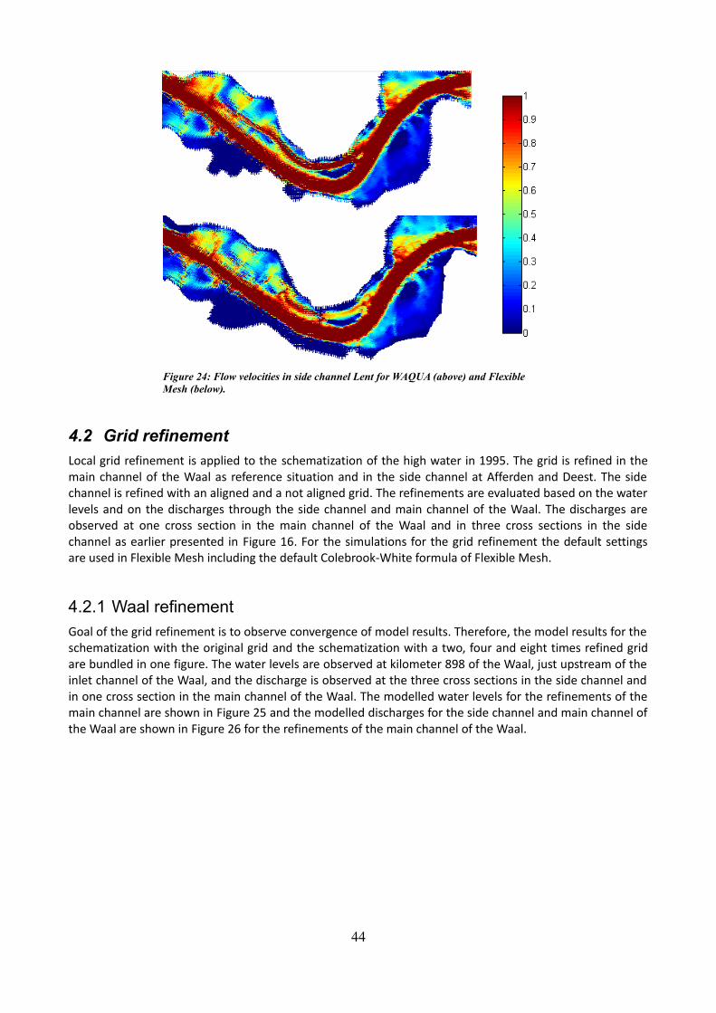
4.2 Grid refinementLocal grid refinement is applied to the schematization of the high water in 1995. The grid is refined in themain channel of the Waal as reference situation and in the side channel at Afferden and Deest. The sidechannel is refined with an aligned and a not aligned grid. The refinements are evaluated based on the waterlevels and on the discharges through the side channel and main channel of the Waal. The discharges areobserved at one cross section in the main channel of the Waal and in three cross sections in the sidechannel as earlier presented in Figure 16. For the simulations for the grid refinement the default settingsare used in Flexible Mesh including the default Colebrook-White formula of Flexible Mesh.

4.2.1 Waal refinementGoal of the grid refinement is to observe convergence of model results. Therefore, the model results for theschematization with the original grid and the schematization with a two, four and eight times refined gridare bundled in one figure. The water levels are observed at kilometer 898 of the Waal, just upstream of theinlet channel of the Waal, and the discharge is observed at the three cross sections in the side channel andin one cross section in the main channel of the Waal. The modelled water levels for the refinements of themain channel are shown in Figure 25 and the modelled discharges for the side channel and main channel ofthe Waal are shown in Figure 26 for the refinements of the main channel of the Waal.

44

Figure 24: Flow velocities in side channel Lent for WAQUA (above) and Flexible Mesh (below).

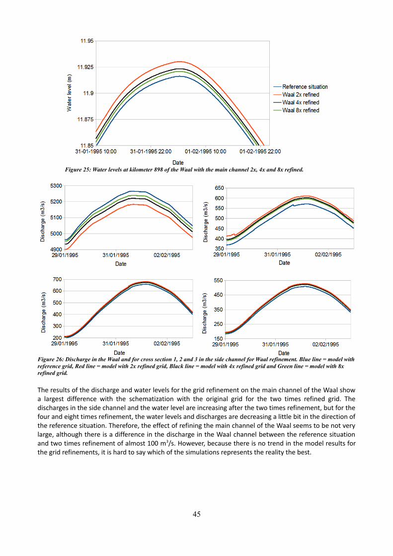
The results of the discharge and water levels for the grid refinement on the main channel of the Waal showa largest difference with the schematization with the original grid for the two times refined grid. Thedischarges in the side channel and the water level are increasing after the two times refinement, but for thefour and eight times refinement, the water levels and discharges are decreasing a little bit in the direction ofthe reference situation. Therefore, the effect of refining the main channel of the Waal seems to be not verylarge, although there is a difference in the discharge in the Waal channel between the reference situationand two times refinement of almost 100 m3/s. However, because there is no trend in the model results forthe grid refinements, it is hard to say which of the simulations represents the reality the best.

45

Figure 25: Water levels at kilometer 898 of the Waal with the main channel 2x, 4x and 8x refined.

Figure 26: Discharge in the Waal and for cross section 1, 2 and 3 in the side channel for Waal refinement. Blue line = model withreference grid, Red line = model with 2x refined grid, Black line = model with 4x refined grid and Green line = model with 8x refined grid.

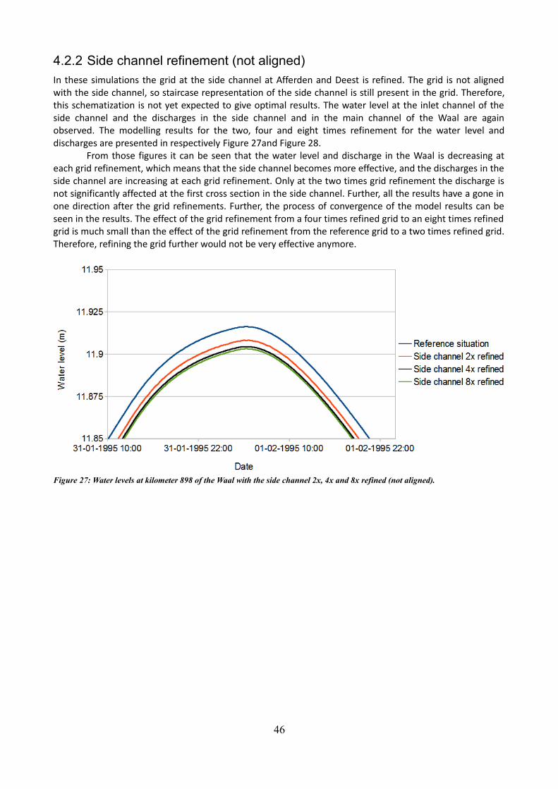
4.2.2 Side channel refinement (not aligned)In these simulations the grid at the side channel at Afferden and Deest is refined. The grid is not alignedwith the side channel, so staircase representation of the side channel is still present in the grid. Therefore,this schematization is not yet expected to give optimal results. The water level at the inlet channel of theside channel and the discharges in the side channel and in the main channel of the Waal are againobserved. The modelling results for the two, four and eight times refinement for the water level anddischarges are presented in respectively Figure 27and Figure 28.

From those figures it can be seen that the water level and discharge in the Waal is decreasing ateach grid refinement, which means that the side channel becomes more effective, and the discharges in theside channel are increasing at each grid refinement. Only at the two times grid refinement the discharge isnot significantly affected at the first cross section in the side channel. Further, all the results have a gone inone direction after the grid refinements. Further, the process of convergence of the model results can beseen in the results. The effect of the grid refinement from a four times refined grid to an eight times refinedgrid is much small than the effect of the grid refinement from the reference grid to a two times refined grid.Therefore, refining the grid further would not be very effective anymore.

46

Figure 27: Water levels at kilometer 898 of the Waal with the side channel 2x, 4x and 8x refined (not aligned).

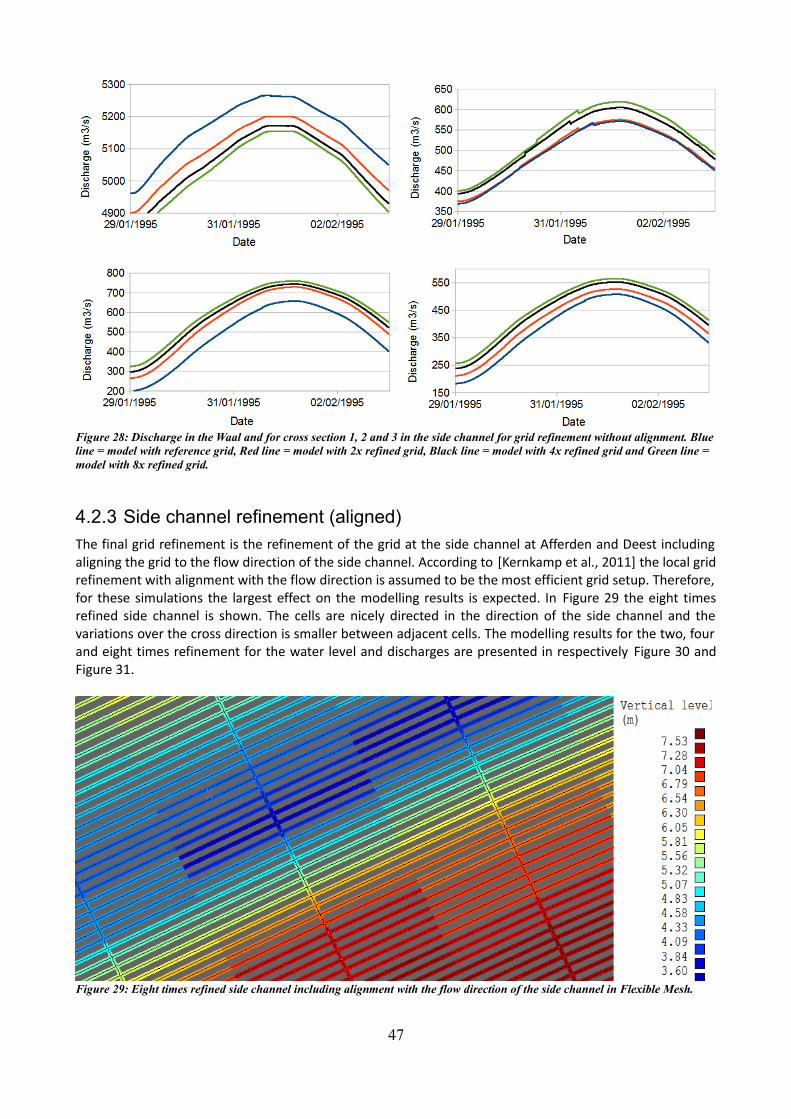
4.2.3 Side channel refinement (aligned)The final grid refinement is the refinement of the grid at the side channel at Afferden and Deest includingaligning the grid to the flow direction of the side channel. According to [Kernkamp et al., 2011] the local gridrefinement with alignment with the flow direction is assumed to be the most efficient grid setup. Therefore,for these simulations the largest effect on the modelling results is expected. In Figure 29 the eight timesrefined side channel is shown. The cells are nicely directed in the direction of the side channel and thevariations over the cross direction is smaller between adjacent cells. The modelling results for the two, fourand eight times refinement for the water level and discharges are presented in respectively Figure 30 andFigure 31.

47

Figure 29: Eight times refined side channel including alignment with the flow direction of the side channel in Flexible Mesh.

Figure 28: Discharge in the Waal and for cross section 1, 2 and 3 in the side channel for grid refinement without alignment. Blueline = model with reference grid, Red line = model with 2x refined grid, Black line = model with 4x refined grid and Green line = model with 8x refined grid.

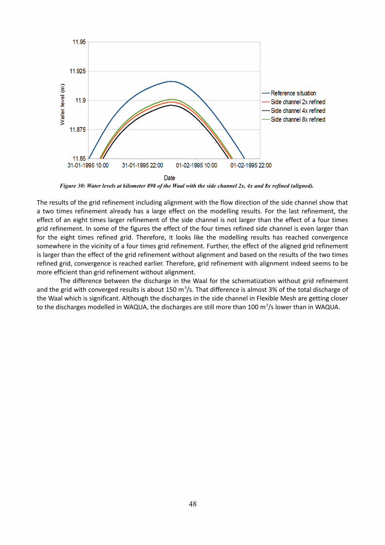
The results of the grid refinement including alignment with the flow direction of the side channel show thata two times refinement already has a large effect on the modelling results. For the last refinement, theeffect of an eight times larger refinement of the side channel is not larger than the effect of a four timesgrid refinement. In some of the figures the effect of the four times refined side channel is even larger thanfor the eight times refined grid. Therefore, it looks like the modelling results has reached convergencesomewhere in the vicinity of a four times grid refinement. Further, the effect of the aligned grid refinementis larger than the effect of the grid refinement without alignment and based on the results of the two timesrefined grid, convergence is reached earlier. Therefore, grid refinement with alignment indeed seems to bemore efficient than grid refinement without alignment.

The difference between the discharge in the Waal for the schematization without grid refinementand the grid with converged results is about 150 m3/s. That difference is almost 3% of the total discharge ofthe Waal which is significant. Although the discharges in the side channel in Flexible Mesh are getting closerto the discharges modelled in WAQUA, the discharges are still more than 100 m3/s lower than in WAQUA.

48

Figure 30: Water levels at kilometer 898 of the Waal with the side channel 2x, 4x and 8x refined (aligned).

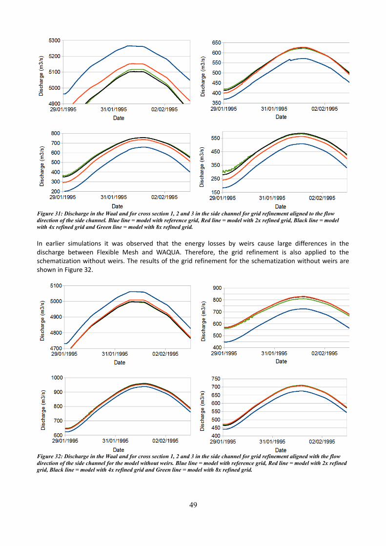
In earlier simulations it was observed that the energy losses by weirs cause large differences in thedischarge between Flexible Mesh and WAQUA. Therefore, the grid refinement is also applied to theschematization without weirs. The results of the grid refinement for the schematization without weirs areshown in Figure 32.

49

Figure 31: Discharge in the Waal and for cross section 1, 2 and 3 in the side channel for grid refinement aligned to the flow direction of the side channel. Blue line = model with reference grid, Red line = model with 2x refined grid, Black line = model with 4x refined grid and Green line = model with 8x refined grid.

Figure 32: Discharge in the Waal and for cross section 1, 2 and 3 in the side channel for grid refinement aligned with the flow direction of the side channel for the model without weirs. Blue line = model with reference grid, Red line = model with 2x refined grid, Black line = model with 4x refined grid and Green line = model with 8x refined grid.

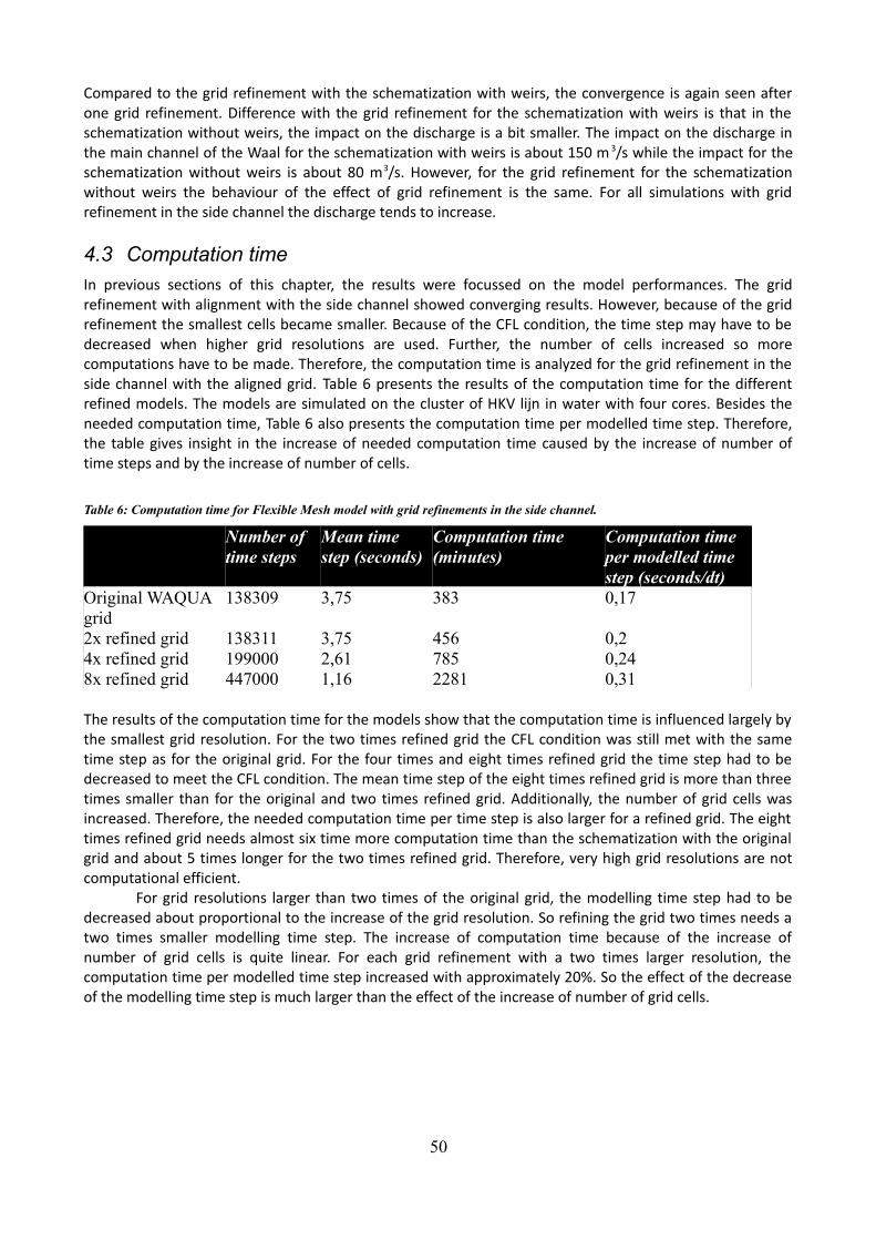
Compared to the grid refinement with the schematization with weirs, the convergence is again seen afterone grid refinement. Difference with the grid refinement for the schematization with weirs is that in theschematization without weirs, the impact on the discharge is a bit smaller. The impact on the discharge inthe main channel of the Waal for the schematization with weirs is about 150 m 3/s while the impact for theschematization without weirs is about 80 m3/s. However, for the grid refinement for the schematizationwithout weirs the behaviour of the effect of grid refinement is the same. For all simulations with gridrefinement in the side channel the discharge tends to increase.

4.3 Computation timeIn previous sections of this chapter, the results were focussed on the model performances. The gridrefinement with alignment with the side channel showed converging results. However, because of the gridrefinement the smallest cells became smaller. Because of the CFL condition, the time step may have to bedecreased when higher grid resolutions are used. Further, the number of cells increased so morecomputations have to be made. Therefore, the computation time is analyzed for the grid refinement in theside channel with the aligned grid. Table 6 presents the results of the computation time for the differentrefined models. The models are simulated on the cluster of HKV lijn in water with four cores. Besides theneeded computation time, Table 6 also presents the computation time per modelled time step. Therefore,the table gives insight in the increase of needed computation time caused by the increase of number oftime steps and by the increase of number of cells.

Table 6: Computation time for Flexible Mesh model with grid refinements in the side channel.

Number of time steps

Mean time step (seconds)

Computation time (minutes)

Computation time per modelled time step (seconds/dt)

Original WAQUA grid

138309 3,75 383 0,17

2x refined grid 138311 3,75 456 0,24x refined grid 199000 2,61 785 0,248x refined grid 447000 1,16 2281 0,31

The results of the computation time for the models show that the computation time is influenced largely bythe smallest grid resolution. For the two times refined grid the CFL condition was still met with the sametime step as for the original grid. For the four times and eight times refined grid the time step had to bedecreased to meet the CFL condition. The mean time step of the eight times refined grid is more than threetimes smaller than for the original and two times refined grid. Additionally, the number of grid cells wasincreased. Therefore, the needed computation time per time step is also larger for a refined grid. The eighttimes refined grid needs almost six time more computation time than the schematization with the originalgrid and about 5 times longer for the two times refined grid. Therefore, very high grid resolutions are notcomputational efficient.

For grid resolutions larger than two times of the original grid, the modelling time step had to bedecreased about proportional to the increase of the grid resolution. So refining the grid two times needs atwo times smaller modelling time step. The increase of computation time because of the increase ofnumber of grid cells is quite linear. For each grid refinement with a two times larger resolution, thecomputation time per modelled time step increased with approximately 20%. So the effect of the decreaseof the modelling time step is much larger than the effect of the increase of number of grid cells.

50

5 DiscussionResults in this study for the comparison between WAQUA and Flexible Mesh showed that the Flexible Meshmodels predict the water levels in the same order as WAQUA when using the same input for theschematization. For low discharges the water levels are almost equal and for high discharges the waterlevels in Flexible Mesh are about 10 centimeter higher. However, the distribution of the discharge over themain channel of the Waal and the floodplain are different. In WAQUA the discharge over the floodplain ishigher than in WAQUA. Moreover, the discharge through the side channel at Afferden and Deest is muchlarger in WAQUA than in Flexible Mesh. An analysis of the differences between WAQUA and Flexible Meshshowed that the Colebrook-White formula and the modelling of energy losses by flow over weirs, which aredifferent for both models, are an important factor for the differences between WAQUA and Flexible Mesh.

For the study of local grid refinements, the grid refinement was applied to the side channel and themain channel at Afferden and Deest. The results show that the effect of the grid refinement to the Waalchannel is limited. The refinement in the side channel has a much larger effect with a difference with theoriginal grid of almost 3% on the discharge through the main channel of the Waal. Further, convergence wasobserved of the modelling results around a two to four times refined grid so the effect of grid refinementdecreased at higher resolutions. Moreover, the computation time of the Flexible Mesh model increased forhigh grid resolutions in the side channel.

5.1 Interpretation results comparisonThe comparison between WAQUA and Flexible Mesh is executed with input data from the calibratedWAQUA model. In Flexible Mesh the same input data was used as in the WAQUA model. Because the sameinput data was used, the expectation was that the differences between WAQUA and Flexible Mesh aresmall. However, the water levels of the Flexible Mesh model deviated from the WAQUA model and themeasurements with about 10 centimeter for high discharges. It cannot be said that the WAQUA model istherefore more accurate than the Flexible Mesh model. The WAQUA model is calibrated on themeasurements so the difference between the measurements and the WAQUA model is minimized.Differences between the WAQUA and Flexible Mesh model will logically result in a deviation of the modelresults in Flexible Mesh from the measurements. In this study the Flexible Mesh model was not calibratedbecause of limited available time. A better image of the accuracy of both models can be obtained bycomparing WAQUA and Flexible Mesh for a testcase in which both models are calibrated. The differencesbetween the measurements and the results of Flexible Mesh are possibly within the range to minimize thedifferences by recalibrating the Flexible Mesh model.

The Flexible Mesh model gave much smaller discharges in the floodplain and discharges in the sidechannel at Afferden and Deest than the WAQUA model. The difference can be attributed for a large part tothe difference in the weir formulation in the model. According to [Warmink et al., 2011], weirs formulation,schematization and discretization is one of the dominant uncertainties in the WAQUA model for the Waal.Therefore, it is important to determine which of the formulations for the weirs in WAQUA and FlexibleMesh are more accurate. In a study of [Gerritsen et al., 2007] the weir formulation in Delft3D is validated.The validation showed that two different advection schemes are available in Delft3D to compute the flowover a weir. One of the schemes was quite accurately within 5% of the analytical discharge, but the otheradvection schemes computed much larger discharges. Because, the Flexible Mesh model is part of theDelft3D suite, in Flexible Mesh the role of weirs might also be influenced by the advection scheme inFlexible Mesh. Therefore, it might be interesting to investigate the influence of numeric settings on thecalculation of flow over weirs.

The second important factor for differences between WAQUA and Flexible Mesh is the Colebrook-White formula. In Flexible Mesh default a different Colebrook-White formula is used than in WAQUA.However, in Flexible Mesh a setting is available to use the WAQUA formulation for the Colebrook-Whiteformula. In this study the WAQUA Colebrook-White formula is used as setting in Flexible Mesh for thecomparison between WAQUA and Flexible Mesh, because the goal of the comparison was to investigate

51

differences in results by numerics. Because the friction is larger when using the Flexible Mesh Colebrook-White formula, the water levels would be higher with the default setting, so the difference betweenWAQUA and Flexible Mesh would be larger. If the Flexible Mesh model will be validated, it would be betterto use the default settings.

5.2 Interpretation results grid refinementThe grid refinement in Flexible Mesh at the side channel at Afferden and Deest showed promising results.While the impact of grid refinement for the main channel showed limited effects, the grid refinement forthe side channel showed quite large effects on the discharges through the side channel and alsoconvergence of the modelling results was observed. These results agree with the expectations, because theWAQUA grid was assumed to be not an accurate representation for the side channel. However, somelimitations are present for the study of the grid refinement.

In the study the original grid was refined locally. With the current tools it is only possible to definethe source data, available in baseline, via the WAQUA model on the original grid. The input data of thebathymetry and bed roughness was for the refined parts of the grid interpolated to the network. Therefore,increasing the grid resolution does not mean that the input data is schematized more accurate. Whenvariations are very large between two points with elevation data, interpolation between both points doesnot accurately represent the elevation within the two points. Therefore, the grid refinement in this studyrepresents the increasing accuracy for calculating the flow and not the increasing accuracy of theschematization. However, bathymetry and roughness are two important factors of uncertainty [Warmink etal., 2011]. Therefore, it would be interesting to investigate what the impact of grid refinement is for a casewhere the bathymetry is also represented more accurate. It is planned to release a version of Baseline inwhich the source data can be attributed to an unstructured grid, which increases the possibilities for gridrefinement in Flexible Mesh. Further, in the schematization with the structured grid the roughness isdefined using trachytope files. However, it is not possible to use the trachytope files for the unstructuredgrid. Therefore, a constant input based on simulations with the original schematization is used as input.Trachytopes define the roughness for a grid cell based on the characteristics of the land in the cell (e.g.vegetation). For accuracy matters, schematization could be improved by defining the trachytope roughnesson the unstructured grid.

The results of the grid refinement in the side channel show positive signals as convergence of themodelling results is observed. The discharges are increased in the side channel with about 100 m3/s asresult of the grid refinement. However, as for the side channel at Afferden and Deest no measurements areavailable. Therefore, it cannot be said with certainty that the grid refinements increase accuracy. Moreover,the differences in discharge through the side channel are large between the WAQUA and Flexible Meshmodel. To better quantify the performances of the Flexible Mesh model, more case studies are desired.Validation of the Flexible Mesh model could be improved to model Flexible Mesh for an existing sidechannel or with a scale model where measurements are available.

Finally, the grid refinement influenced the needed computation time of the Flexible Mesh model.For large grid resolutions the modelling time step had to be decreased. Long computation time is oftenundesirable. Moreover, the results showed that grid refinement at higher grid resolutions have less impacton the model results. Therefore, grid refinement is especially efficient for grids with low resolution.Evaluation if grid refinement is useful for a specific case can be based on variations in the bathymetry orroughness in the case, the used grid resolution and if the grid is aligned with the flow direction of the river.The CFL criteria can be used to estimate whether the time step is influenced by a grid refinement. Further,the computation time has increased because the number of grid cells increased after a grid refinement. Inthis study the grid refinement was only applied to the Afferdense and Deestse floodplains. The computationtime increased with 20% for a two times larger grid resolution at Afferden and Deest, which is stillacceptable. When simulating a larger model, for example the Rhinemodel, local grid refinement might bedesired at multiple locations. Therefore, the increase of computation time would increase more than in thisstudy. However, because the Rhinemodel is much larger the relative increase will probably be comparable

52

to the increase of computation time in this study. Further, in this study only grid refinement is applied. Theunstructured grid possibilities of Flexible Mesh also enables the modeller to coarsen the grid locally on thelocations which might need less accurate schematization. Grid coarsening might be applied to compensatefor the increase of computation time by grid refinement.

5.3 Practical application of Flexible MeshThe effect of the local grid refinement on the discharge in the main channel of the Waal, about 3% of thedischarge, is significant. Such a difference might have a large long term impact on the morphology of theriver, because of changes in sedimentation at the inlet and outlet of the side channel. Such differences inthe results of a hydrodynamic model might have a large impact on the decision which will be made in rivermanagement, for example for the design of a side channel. Therefore, the hydrodynamic models should bereliable and accurate.

Results of Flexible Mesh in this study seem to be promising. As an effect of local grid refinements inthe side channel at Afferden and Deest, the discharge in the side channel tends to increase. The effect ofgrid refinements on the discharge in the main channel of the Waal is quite large. Further, the effect of thegrid refinement was small for large grid resolutions which indicate that the model results have converged.These results indicate that the accuracy of the computation of the flow in the side channel is improved bythe local grid refinement.

Although the accuracy of WAQUA and Flexible Mesh is not assessed in this study, the local gridrefinements in Flexible Mesh seem to improve the accuracy of the computation of the flow in the sidechannel. Compared to the WAQUA grid the grid refinement improves on the staircase representation of theside channel, because the grid was aligned with the flow direction of the side channel. Further, thevariations between adjacent grid cells were smaller because of the higher grid resolution. Therefore, theunstructured grid of Flexible Mesh can help to improve the reliability of model results for complexgeometries in future.

53

6 Conclusions and recommendationsThis research focussed on the modelling in Flexible Mesh with the side channel at Afferden and Deest asstudy case. The aim of this research was to compare modelling results of WAQUA and Flexible Mesh andcauses for differences between the models and to investigate the impact of local grid refinement in FlexibleMesh on the modelling results. This chapter summarizes the most important results of the study andconclusions are drawn. Further, recommendations are given based on the results of this study.

6.1 ConclusionsWhat causes differences between WAQUA and Flexible Mesh?

There are two important sources for the differences between WAQUA and Flexible Mesh. First, FlexibleMesh default uses a different formula for the Colebrook-White roughness which results in a larger friction inFlexible Mesh. The effect of the Colebrook-White formula is an about 15 centimeters higher water level inFlexible Mesh. Second, the energy losses due to flow over weirs is modelled different in Flexible Mesh,which results in almost 10 centimeter higher water levels in Flexible Mesh and lower discharges in thefloodplain. Further, in Flexible Mesh the bed level between two bed level points can be represented with adiagonal while in WAQUA the bed level between two bed level points is always horizontal. The effect of therepresentation of the bed level between two bed level points can be about five centimeters. Last thin damscause a difference of circa two centimeters between WAQUA and Flexible Mesh. When these differencesare left out, the water level in WAQUA and Flexible Mesh are comparable with a maximal difference of 2centimeters. So the numerical performance of WAQUA and Flexible Mesh seems to be quite similar.

What are the differences in water levels, flow velocities and discharges between WAQUA and Flexible Mesh?

The results of the water levels in the Flexible Mesh model are comparable to the results of the water levelsin the calibrated WAQUA model for the Waal. For low discharges the difference of the water level is lessthan one centimeter, but for high discharges the water levels are higher in the Flexible Mesh model. Thedifference between the water level in the WAQUA model and Flexible Mesh model is about 12 centimetersat a high discharge. The discharges and flow velocities are different in the Flexible Mesh model compared tothe WAQUA model. Especially the discharge over the floodplains and in the side channel at Afferden andDeest are much smaller in the Flexible Mesh model. The discharge in the side channel at Afferden and Deestis about 200-300 m3/s higher in the WAQUA model compared to the Flexible Mesh model. This is almost 4%of the total discharge in the Waal at the peak, which is significant and might have a large effect on decisionmaking in river management. However, because only the WAQUA model was calibrated it cannot be saidwhich model is more accurate.

What is the effect of local grid refinement in Flexible Mesh on the model results?

Local grid refinement was applied at Afferden and Deest to the main channel of the Waal and to the sidechannel. Although the discharge in the main channel is maximally affected with 100 m3/s, the results do notshow a clear effect of the grid refinement. The two times refined grid showed another trend in the modelresults than the four times and eight times refined grid for the Waal refinement. The grid refinement in theside channel showed larger effects than the grid refinement of the main channel of the Waal on the waterlevel and the discharge. The refinement of the side channel was executed with an aligned and not alignedgrid with the flow direction of the side channel. The aligned grid resulted in the largest effect on the modelresults. The refinement in the side channel results in maximal 150 m 3/s lower discharges in the mainchannel of the Waal and 100 m3/s higher discharges in the side channel compared to the schematizationwith the original grid. The difference with the original grid is maximal for the eight times refined side

55

channel. However, the largest effect of grid refinement is observed at small grid resolutions. After the gridwas refined four times the results are hardly affected by a grid refinement anymore. Therefore,convergence seems to be reached around the four times refined side channel. The observation ofconvergence of model results for grid refinement in the side channel indicates that grid refinementimproves the accuracy of the computation of the flow in the side channel.

Although the grid refinements seem to be promising based on the results, the computational timeincreases because of grid refinement. For high grid resolutions, the time step has to be decreased in orderto meet the CFL condition. Further, the number of grid cells increases so more computations have to bedone. Upward of a two times refinement, the computation time increases more than two times. Therefore,grid refinement is efficient when model results are not yet converged and computational time is stillacceptable.

6.2 RecommendationsThe results of this study show promising results of Flexible Mesh. The application of local grid refinement inFlexible Mesh showed that accuracy can be improved in complex geometries. However, the performance ofFlexible Mesh compared to WAQUA is not well known yet. Below recommendations are presented forfuture application of the unstructured grid of Flexible Mesh and for further research.

– For river areas with an interest to complex geometries like side channels, higher grid resolutionsshould be used than standard used grid resolutions for large scale river models like the Rhinemodelin WAQUA. For this purpose, the unstructured grid based D-Flow Flexible Mesh is an appropriatemodel.

The results for the grid refinements in the side channel at Afferden and Deest showed a trend to convergeto a higher discharge in the side channel. The convergence indicates that the models with higher gridresolutions are more accurate. The effect of the grid refinement at the side channel in Flexible Meshresulted in quite large effects on the discharges in the side channel and the main channel of the Waal. Theobserved effects are significant for morphological effects and therefore for decision making in rivermanagement. D-Flow Flexible Mesh is an appropriate model to use higher grid resolutions, because gridrefinement can be applied to areas where the modeller wants. Therefore, the increase of neededcomputational effort can be limited.

– Grid refinement should be applied for cases in which the effect on the model results is significantand the increase of computation time of the model is still acceptable.

In this study it was observed that the model results converged for local grid refinements in the side channel,so at high grid resolutions grid refinement had almost no effect anymore. Further, the needed computationtime of the model increased because of the grid refinement, especially for large grid resolutions. If the cellsat the grid refinement are getting to small, the CFL condition is not met with the desired time step, so thetime step will be automatically decreased in Flexible Mesh. Moreover, the number of grid cells increasesbecause of grid refinement. The efficiency of grid refinement can be estimated based on the complexity of ageometry compared to the size of grid cells (e.g. variations in bed level between adjacent cells) and theeffect of grid refinement on the needed computation time, based on the smallest grid cell and the CFLcondition.

– The used method for modelling energy losses by weirs and of the used Colebrook-White formula inFlexible Mesh might be validated.

Flexible Mesh uses another method for modelling energy losses by weirs and a different Colebrook-Whiteformula than WAQUA. In this study it was observed that these two issues cause significant differences

56

between the results in the WAQUA and Flexible Mesh model. However, it is not clear which method is moreaccurate. Experiments in which different cases will be explored for the roughness and weirs might give moreinsight in the accuracy of the used method.

– Further research should be done to the accuracy of D-Flow Flexible Mesh regarding the water levelsand regarding the discharges over the floodplain and through a side channel before using D-FlowFlexible Mesh for a real project.

The calculated water levels in the Flexible Mesh model differ significantly from the calibrated WAQUAmodel. It is recommended to calibrate and verify the Flexible Mesh model for the Rhinemodel withmeasurements of the water levels for different discharge regimes, like the WAQUA model was calibrated.Further, the discharges over the floodplain and in the side channel at Afferden and Deest were muchsmaller in Flexible Mesh than in WAQUA. However, in this study no measurements were available for theAfferdense and Deestse floodplains. The discharges over the floodplain and in a side channel might bevalidated for a case study where results of Flexible Mesh can be compared with measurements.

– Further research might be done to assess the effect on model results in Flexible Mesh of increasingthe accuracy of the schematization of the geometry and roughness on a local grid refinement.

In this study the local grid refinement in the side channel at Afferden and Deest improved on staircaserepresentation of the side channel by aligning the grid with the flow direction and improved on thevariations between adjacent cells in the side channel by increasing grid resolution. However, theschematization of original input data was interpolated to the refined grid, so the accuracy of the roughnessand geometry was not improved. When it becomes possible to export data from Baseline directly to theunstructured grid in Flexible Mesh, grid refinement could also be used to improve the accuracy of thegeometry and the roughness in the schematization. It will be interesting to assess the effect of gridrefinement including improving the input data at the local refinement.

57

Literature

Becker, A., 2012 Rijn-modellen 5de generatie: modelopzet, kalibratie en verificatie WAQUA. Deltares report nr. 1205944-02

Van Dam, A., Kernkamp, H.W.J., Van Der Pijl, S., & Van Balen, W., 2014, D-Flow Flexible Mesh: user manual, Delft, The Netherlands: Deltares

Deltares, 2014, Delft3D-flow: user manual. Version 3.15.34158, Delft, The Netherlands: Deltares

DHI, 2011, MIKE 21 flow model fm: user guide, Hørsholm, Denmark: DHI

EDF-R&D, 2013, TELEMAC modelling system: Operating manual, Paris, France: EDF-R&D

Garcia, M.H., 2008, Sedimentation Engineering: processes, measurements, modeling, and practice, Reston, Virginia: American Society of Civil Engineers

Gerritsen, H., De Goede, E.D., Platzek, F.W., Genseberger, M., Van Kester, J.A.Th.M., & Uittenbogaard, R.E., 2007, Validation document Delft3D-flow: a software system for 3D simulations, Delft, The Netherlands: WL | Delft Hydraulics

Gunzburger, M.D., Peterson, J.S., 2013 Finite element methods. Retrieved February 2014, from http://people.sc.fsu.edu/~jburkardt/classes/fem_2011/chapter1.pdf

Herinrichting Afferdense en Deestse Waarden. Retrieved February 2014 from www.rijkswaterstaat.nl

Kernkamp, H.W.J., 2014 DFM opzet Waalmodel. Deltares, Memorandum 15 January 2014, research of minimalization of computation time in Flexible Mesh by using possibilities of the unstructured mesh.

Kernkamp, H.W.J., Van Dam, A., Stelling, G.S., & De Goede, E.D., 2011, Efficient scheme for the shallow water equations on unstructured grids with application to the Continental Shelf, Ocean Dynamics, 61 (8), 1175-1188.

Open Earth Tools. Retrieved March 2014, from https://publicwiki.deltares.nl/display/OET/OpenEarth

Peiró, J., & Sherwin, S., 2005 Finite difference, finite element and finite volume methods for partial differential equations. Retrieved February 2014, from http://imcool.kaist.ac.kr/teaching/PDE_three_views.pdf

Van Der Pijl, 2013. Deltares, Memorandum 8 October 2013, description of simulations of schematic Waal model with D-Flow FM and WAQUA.

Rijkswaterstaat, 2013, User guide WAQUA: general information. Version 10.59, The Netherlands: Rijkswaterstaat

Rijkswaterstaat, 2012, WAQUA/TRIWAQ: two- and three dimensional shallow water flow model. Simona report nr. 99-01, The Netherlands: Rijkswaterstaat

Verwey et al., 2011: Verwey, A., Kernkamp, H.W.J., Stelling, G.S., Tse, M.L., & Leung, W.C., Potential and application of hydrodynamic modelling on unstructured grids. Proceedings of the Sixth International Conference on Asian and Pacific Coasts 2011. Hong Kong

59

Vreugdenhil, 1994, Numerical methods for shallow-water flow, Dordrecht: Kluwer Academic Publishers

Warmink, J.J., Van Der Klis, H., Booij, M.J., & Hulscher, S.J.M.H., 2011, Identification and quantification of uncertainties in a hydrodynamic river model using expert opinions, Water Resources Management, 25 (2), 601-622.

Warmink, J.J., 2009. Literature report: uncertainty analysis of hydrodynamic river models. CE&M research report 2009R-001/WEM-001, University of Twente, Civil Engineering and Management, ISSN 1568-4652.

60

Hydrodynamic river modelling with D-Flow Flexible...

Documents

Transcript of Hydrodynamic river modelling with D-Flow Flexible...