Deterministic and stochastic methods of ... R. Kosova et.al _______________________________________________________________________________________________

 226  

 

Paper presented in 1-st International Scientific Conference on Professional Sciences, “Alexander Moisiu” University, Durres November 2016

DETERMINISTIC AND STOCHASTIC METHODS OF OILFIELD RESERVES

ESTIMATION: A CASE STUDY FROM KA. OILFIELD.

ROBERT KOSOVA1, ADRIAN NAÇO2, IRAKLI PRIFTI2

1Department of Mathematic, Faculty of Technology and Information, “Alexandër Moisiu” University. Durrës. Albania 2Polytechnic University of Tirana. Tirana. Albania

Corresponding e-mail author: robertco60@yahoo.com

Abstract Reserves Estimation is a process that continues during almost all the life of the Oilfield. And it is always affected by uncertainty and errors. The first level of uncertainty is associated with first data taken from geophysical profiles, wells, cores, water etc. These data provide reservoir properties such as areas, depth, porosity, saturation, temperature, etc. The second level of uncertainty is produced when reservoir properties are used in formulas and correlated with the help of geology, seismic and production tests. Reserves-estimation methods are broadly classified as analogy, volumetric and production types. The choice of methodology depends on timing of development and production, amount of data, reservoir characteristics. Analogy Method is the simplest is based on geologic analogy with a nearby producing area. The method is reliable to the extent that the analogy is valid, which can be estimated by statistical test. The two volumetric methods for Reserves estimation are deterministic and stochastic, (Derminem F., 2007). In case of deterministic method, mathematical formulas are used to estimate volumes or reserves. The stochastic method considers the fact that each parameter is not presented with a single value, but is included in an interval of values and fit a probability distribution which is to be found out, estimated and used properly, (Prifti I, Kosova R., 2014). The results from stochastic calculations are concluded generally by a reverse cumulative probability function, the expectation curve, (Wadsley A. W., 2011). We will use both, deterministic and stochastic methods, in estimating reserves in the case study of KA. Oilfield. Key words: Reserves, probability, estimation, deterministic, stochastic, analogy, volumetric, oilfield

Introduction: Risk and uncertainty are always present in the oil and gas industry. Oil and gas reservoirs are in most cases irregular rock structures and shapes and hydrocarbon content is not uniformly distributed. The collected data represent only a small fraction of their values and distribution and, from such data we must draw conclusions for the whole volume of oil- gas reservoir rock. As a result of restrictions on getting all the data we need, in terms of quantity and quality, it is very difficult to have a complete picture of the characteristics of each oil- gas reservoir. In every project development in oil industry, always accompanied with a portfolio worth several million euros, it is understandable that we are dealing also with a great financial risk, due to uncertainty and complicated nature of oil

projects. The process of reserves estimation is a function of time and reserves, because there will always be uncertainty in making reserves estimates. The uncertainty and level of uncertainty is affected and determined by the main following factors: 1. Reservoir type of oilfield, 2. Source of reservoir energy, 3. Quantity and quality of the geological,

engineering, geophysical data and other related data,

4. Assumptions made as a result of estimating process,

5. Available technology and estimating programs,

6. Experience and knowledge of the reserves evaluators, simulations and modelling.

Interdisplinary Journal of Research and Development “Aleksandër Moisiu“ University, Durrës, Albania Vol (IV), No.2, 2017 ________________________________________________________________________________________________

 227  

 

The magnitude of uncertainty, however, decreases with time until the relative economic limit is reached, which is a function of fiscal rules, production costs, international conditions and markets, and the ultimate recovery is realized;that is the end of oilfield active life, Figure 1.

Figure1. Changes in uncertainty and assessment

methods. 1) Classifications of Reserves: (SPE 2007, SPE

2011). Reserves are estimated remaining quantities of oil and gas natural and related substances anticipated to be commercially recovered from known accumulation from a given date forward under defined conditions: • Analyses of drilling, geological, and

engineering data, • The use of present technology, • Specified economic condition, which are

accepted as being reasonable.

Reserves are classified according to the degree of certainty associated with the estimates. Proven Reserves are those reserves that have a reasonable certainty (normally at least 90% confidence) of being recoverable under existing economic and political conditions, with the present existing technology and state regulations. Oil industry specialists refer to this as P90 or 1P. Probable Reserves are those reserves that have

a reasonable certainty (normally at least 50% confidence) of being recoverable under existing economic and political conditions, with the present existing technology and state regulations. Oil industry specialists refer to this as P50 or 2P. Possible Reserves are those reserves that have a reasonable certainty (normally at least 10% confidence) of being recoverable under existing economic and political conditions, with present existing technology and state regulations. Oil industry specialists refer to this as P10 or 3P, figure 2.

Figure 2. Reserves Estimates Classification.

2. Classification of Reserves Estimation Methods.

The oil and gas reserves estimation methods can be classified into the following categories:

1. Analogy method of estimation, 2. Volumetric method of estimation, 3. Decline analysis of production curve, 4. Material balance calculations for oil and

gas reservoirs, 5. Oilfield Reservoir simulation,

In the early stages of project development, reserves estimates are restricted to the analogy and volumetric method of estimation. The analogy method is applied by comparing factors for the analogous and current fields or wells. An almost abandoned oilfield, for which we have the best and maximum knowledge of its geological data, producing life and reserves estimation,is taken in consideration as an approximate to the current new oilfield. This method is most useful when

Deterministic and stochastic methods of ... R. Kosova et.al _______________________________________________________________________________________________

 228  

 

running the economics estimation facts on the new oilfield; which is supposed to be an exploratory oilfield, we know a little about its reserves capacities.It is important anyway, to have the best of geological similarities between new oilfield and the old one, in terms of sedimentary rock types; theoilfields mustbe includedin the same type of oil fields rock which are; shale’s, sandstones, and carbonates.The volumetric method, on the other hand, is about estimating the reserves estimation from the volumetric rock data, the area, the thickness, pore volume and other important data as oil or water saturation, porosity, and the fluid content within the pore volume. This provides an estimation of the amount of hydrocarbons-in-place in volumetric unit or tons. The ultimate recovery, then, can be estimated by using an appropriate recovery factor, because not all the oil in place can be recovered from the reservoir.As production and pressure data from a field become available, methods of decline analysis and material balance become the most used methods of reserves estimations.These estimating methods greatly reduce the uncertainty in reserves estimates by being more accurate, because we use can use much more geological and production data. Decline curve analysesisbased on daily production data, (Arps, 1945, 1956).The technique is not necessarily grounded in fundamental theory but is based on empirical observation of oilfield production decline.Three types of declines that are observed are;

1. Exponential 2. Hyperbolic 3. Harmonic

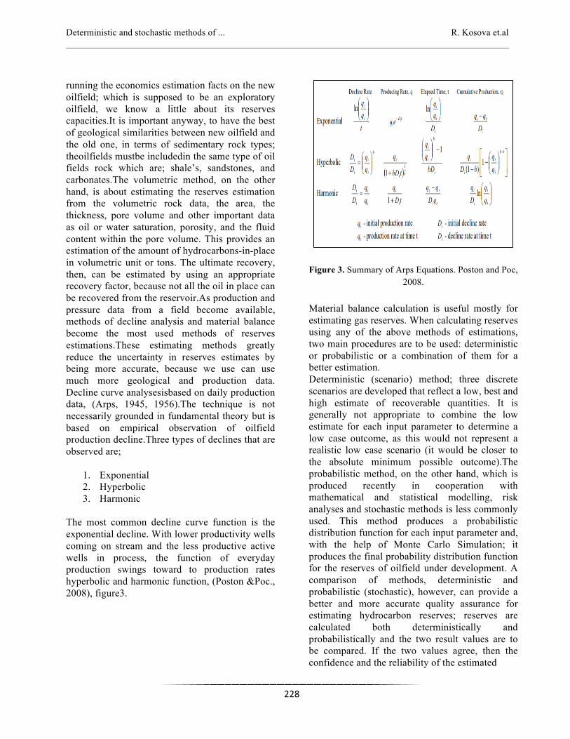
The most common decline curve function is the exponential decline. With lower productivity wells coming on stream and the less productive active wells in process, the function of everyday production swings toward to production rates hyperbolic and harmonic function, (Poston &Poc., 2008), figure3.

Figure 3. Summary of Arps Equations. Poston and Poc, 2008.

Material balance calculation is useful mostly for estimating gas reserves. When calculating reserves using any of the above methods of estimations, two main procedures are to be used: deterministic or probabilistic or a combination of them for a better estimation. Deterministic (scenario) method; three discrete scenarios are developed that reflect a low, best and high estimate of recoverable quantities. It is generally not appropriate to combine the low estimate for each input parameter to determine a low case outcome, as this would not represent a realistic low case scenario (it would be closer to the absolute minimum possible outcome).The probabilistic method, on the other hand, which is produced recently in cooperation with mathematical and statistical modelling, risk analyses and stochastic methods is less commonly used. This method produces a probabilistic distribution function for each input parameter and, with the help of Monte Carlo Simulation; it produces the final probability distribution function for the reserves of oilfield under development. A comparison of methods, deterministic and probabilistic (stochastic), however, can provide a better and more accurate quality assurance for estimating hydrocarbon reserves; reserves are calculated both deterministically and probabilistically and the two result values are to be compared. If the two values agree, then the confidence and the reliability of the estimated

Interdisplinary Journal of Research and Development “Aleksandër Moisiu“ University, Durrës, Albania Vol (IV), No.2, 2017 ________________________________________________________________________________________________

 229  

 

reserves method is increased. If the two values are away different, then the process and the methods are to be reconsidered.

6. Volumetric Method and the Input reservoir parameters:

The volumetric method need the data from the physical size of the reservoir, the rock pore volume within the rock matrix, and the fluid content within the void space. This will provide an estimate of the hydrocarbons-in-place, from which we can estimate the ultimate recovery by using an appropriate recovery factor.

𝑂𝑂𝐼𝑃 = 𝑄𝑝𝑟𝑜𝑣   =  𝑆   ∗  �  m ∗𝑚   ∗  𝑆𝑛   ∗  𝑌𝑛   ∗  1  /  𝑏𝑛 (1)            𝑈𝑅

=  𝑂𝑂𝐼𝑃∗  𝑅𝐹                                                                                                                                                                  (2) OOIP = Oil Originated in Place (Geological Reserves). UR = Ultimate Recovery (Primary Recoverable Reserves). 𝑄 = Oil Reserves (tons), 𝑆 = Oilfield area (𝑚!), �𝑚= Average depth of reservoir (m), 𝑚 = Porosity ratio (%); it is the ratio of the volume of space to the total volume of a rock. 𝑆𝑛 = Oil saturation (%); the relative amount of oil and gas in the pores of a rock, usually as a percentage of volume. 𝑌𝑛 = Density of oil (!"

!!);mass per unit of oil volume. 𝑏𝑛 = Formation Volume Factor; oil and dissolved gas volume at reservoir conditions divided by oil volume at standardconditions. Oil formation volume factor is almost always greater than 1. 𝑅𝐹= Recovery Factor. For primary recovery (natural depletion), the RF is less than 20% in most cases. For secondary recovery, RF ranges from 15 to 25%.

7. Monte Carlo simulation: Monte Carlo technique consists of generating random values after specific probability distributions. The random generation and, the reserves estimation can be done by using software

such as Crystal Ball (2007), @Risk, Minitab, Easy Fit, which are frequently used in estimating risks in investment, financial sectors, petroleum reserves and mining evaluation. By the central- limit theorem, the result (oilfield reserves) of sum of independent distribution approaches normal distribution, regardless of the type of input variables and; the multiplication of independent distributions approaches lognormal distribution, regardless of the type of input variables. Therefore, which is our case, the distribution of assume reserves will be lognormal.

8. KA- Oilfield Case Study. Estimating the Parameters Distributions: The porosity is usually assigned a log normal distribution following the observations of Cronquist, (2001) quoting Arps and Roberts, (1958) and Kaufmann, (1963); in a given geologic setting, a log normal distribution is a reasonable approximation to the frequency distribution of field size, i.e., to the ultimate recoveries of oil or gas and other geological or engineering parameters like porosity, permeability, water saturation and net pay thickness, the oil density parameter is considered triangular distribution, porosity and oil saturation distributions values are considered lognormal or triangular, permeability and thickness are considered triangular or uniform, depended from the oilfield data, table1. Table1. Partial Data of KA- D sector. Oilfield parameters and their probability distributions. Oil

density Reservoir

area Porosity Oil

saturation

Permeability Thickness

KA1 0.88 2,800,500m2

10%- 30% 29% 1 245 m

KA2 0.91 3,800,100 m2

8%- 26% 40% 0.9 440 m

KA3 0.93 2,900,800 m2

10%- 33% 30% 0.8 290 m

KA4 0.85 2,600,500 m2

4%- 22% 35% 1 480 m

KA5 0.86 2,100,500 m2

7%-28% 25% 0.7 323 m

KA6 0.89 1,800,300 m2

7%-30% 42% 0.9 625m

Average 0.89 2,300,400m2 18% 33.5% 0.88 400 m

Intervals 0.5-0.95

1.5- 4,000,000

1%-35%

10%-50% 0.6-1 200-700

Distribution

triangular triangular lognor

mal lognor

mal triangula

r triangular

Parameters

(.5; .85; .95) (1.5; 3; 5) (18; 5) (25; 10) (.6; .76;

1) (200;500;7

00)

Results:

Deterministic and stochastic methods of ... R. Kosova et.al _______________________________________________________________________________________________

 230  

 

The generation of random values (5000) after the parameters data and their estimation distributions if performed by Minitab 17, figure 4. The data are stored in 1-5 columns in order to produce the multiplication of them, after the formula (1), (2). The result is the probability distribution of Reserves and the Cumulative Reserves, figure 5.

Figure 4. Probability distribution of Oil density and Area parameters.

Reserves Estimates for 1P, 2P, 3P: The probability that the output (Reserves) is greater than or equal to 2 M tons is 90 % (Proven reserves), 𝑝(𝑅 ≥ 2𝑀  𝑡𝑜𝑛) = 90%. The probability that the output (Reserves) is greater than or equal to 7 M tons is 50 % (Proven + Probable Reserves, Mode or Most Likely),𝑝(𝑅 ≥ 7𝑀  𝑡𝑜𝑛) = 50%. The probability that the output (Reserves) is greater than or equal to 22 M tons is 10 % (Proven + Probable + Possible or Maximum Reserves), 𝑝(𝑅 ≥ 22𝑀  𝑡𝑜𝑛) = 10%.

Figure 5. PDF of Reserves and Cumulative Reserves. Conclusions

• In this study, we try to re-evaluate the reservoir of KA- D sector oilfield, using the probability method of reserves estimation, by using Monte Carlo Simulation.

• Monte Carlo Simulation can be was successfully be applied to the real oilfield. Before applying the M. C. simulation, it is important to have the most accurate data provided by the oilfield, the well cores, geologic data, and the best probability distribution approximation of basic reservoir characteristics (net thickness of rock and gas sand and averaged porosity).

• The probability distributions are produced by best estimation of theoretical knowledge and oilfield laboratory data.

• In applying Monte Carlo Simulation method, the volume estimation is also obtained considering the heterogeneity of the reservoir property over the field.

• Reserves estimation, produced by the formula (1) will be multiplied by the oil

0.900.840.780.720.660.600.54

80

70

60

50

40

30

20

10

0

Oil  density  parameter;  .5;  .85;  .95

Freq

uenc

y

H istogram  of  oil  Density.

5.04.54.03.53.02.52.01.5

70

60

50

40

30

20

10

0

Reservoir  Areas,  parameters-­‐  1.5;3;5.

Freq

uenc

y

H istogram  of  Reservoir  Area.

96000008400000720000060000004800000360000024000001200000

500

400

300

200

100

0

Loc 15.00Scale 0.3022N 5000

Reserves

Freq

uenc

y

Lognormal  H istogram  of  Reserves  Distribution

10000000

9000000

8000000

7000000

6000000

5000000

4000000

3000000

2000000

1000000

100

80

60

40

20

0

Loc 15.00Scale 0.3022N 5000

Cumulative  Reserves

Percen

t

Lognormal  Empirical  CDF  of  Reserves

Interdisplinary Journal of Research and Development “Aleksandër Moisiu“ University, Durrës, Albania Vol (IV), No.2, 2017 ________________________________________________________________________________________________

 231  

 

formation volume factor,1/bn. For oil is less than 1, for gas is greater than 1. The factor represents the volume of oil and gas in natural condition divided by the volume under the earth. Oil shrinks, gas enlarges its volume.

References [1] ARPS J, ROBERTS T. G (1958) Economics of drilling for Cretaceous oil on the east flank of the DenverJulesburg Basin. American Association of Petroleum Geologists Bulletin. 42: 2549-2566. [2] PRIFTI I (1995) Generation model of hydrocarbon in limestone section penetrated from Ballshi-27 well by maceral analyses and vitrinites reflectance. In: “Albanian oil ”magazine, nr. 4. [3] VELAJ T, PRIFTI I(1996)On hydrocarbon potential in Albania. In: 2nd International Symposium on the Petroleum Geology and Hydrocarbon Potential of the Black Sea Area. Istanbul, Turkey [4] CAPEN E. C(1992) Dealing with Exploration Uncertainties. In The Business of Petroleum Exploration, ed. R. Steinmetz, Tulsa: American Assn. Petroleum Geologists, 29–61. [5] CRONQUIST C (2001) Estimation and Classification of Reserves of Crude Oil, Natural Gas, and Condensate. Richardson, Texas: Society of Petroleum Engineers. 416. [6] DEMIRMEM F (2005) Reliability and Uncertainty in Reserves: How and Why the Industry Fails, and a Vision for Improvement. Paper SPE 94680 presented at the SPE Hydrocarbon Economics & Evaluation Symposium, Dallas, 3–5 April. DOI: 10.2118/94680-MS. [7] Petroleum Reserves Definitions (1997) Richardson, Texas: Societyof Petroleum Engineers. http://www.spe.org/spe/jsp/basic/. [8] KOSOVA R, NACO A (2015)"Uncertainty in Oil Reservoir Properties Deterministic and Stochastic Methods of Reserves Estimation". IJSR Archive Volume 4 Issue 10 October 2015: Pages: 471-474.

[9] https://www.ijsr.net/archive/v4i10/v4i10.php. [10] WADSLEY A. W (2011) Markov Chain Methods for Reserves Estimation. International Petroleum Technology Conference. Doha, 2005. 6 pp. [11] KOSOVA R, SHEHU V, NACO A (2015) Monte carlo simulation for estimating geologic oil reservs. A case study from Kuçova oilfield in Albania, MuzeulOlteniei Craiova. Oltenia. Studiişicomunicări. ŞtiinţeleNaturii. Tom. 31, No. 2, ISSN 1454-6914 20.