Determination of Forward and Futures...
39
Determination of Forward and Futures Prices Chapter 5 1
Transcript of Determination of Forward and Futures...

Determination of Forward and Futures Prices
Chapter 5
1

Consumption vs Investment Assets
l Investment assets are assets held by a significant number of people purely for investment purposes(Examples: stocks, bonds, gold, silver – although a few people might also hold them for industrial purposes for example).
l Consumption assets are assets held primarily for consumption (Examples: copper, oil, pork bellies) and not usually for investment purposes.
l Arbitrage arguments will not work the same way for consumption assets as they do for investment assets.
2
Short Selling (Page 105-106)
l Short selling or “shorting” involves selling securities you do not own.
l Your broker borrows the securities from another client and sells them in the market in the usual way.
3

Short Selling (continued)
l At some stage you must buy the securities so they can be replaced in the account of the client.
l You must pay dividends and other benefits the owner of the securities receives.
l There may be a small fee for borrowing the securities.
4

Example
l You short 100 shares when the price is $100 and close out the short position three months later when the price is $90.
l During the three months a dividend of $3 per share is paid.
l What is your profit?
l What would be your loss if you had bought 100 shares?
5
Example
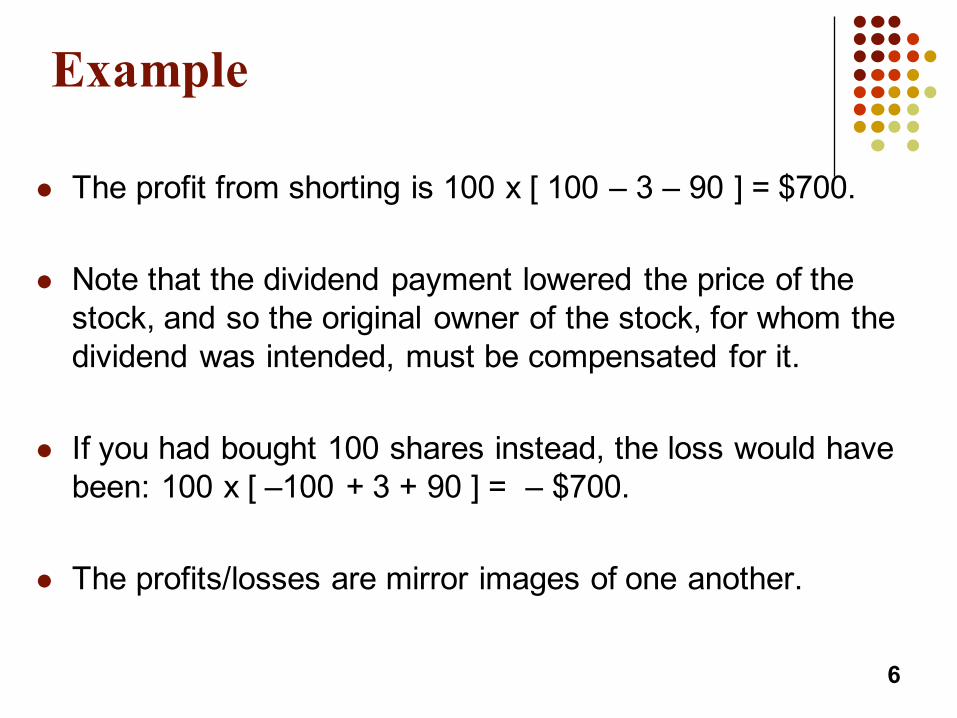
l The profit from shorting is 100 x [ 100 – 3 – 90 ] = $700.
l Note that the dividend payment lowered the price of the stock, and so the original owner of the stock, for whom the dividend was intended, must be compensated for it.
l If you had bought 100 shares instead, the loss would have been: 100 x [ –100 + 3 + 90 ] = – $700.
l The profits/losses are mirror images of one another.
6

Notation for Valuing Futures and Forward Contracts
7
S0: Spot price today
F0: Futures or forward price today
T: Time until delivery date (expressed in years)
r: Risk-free interest rate for maturity T (also expressed in years)

An Arbitrage Opportunity?
l Suppose that:l The spot price of a non-dividend-paying
stock is $40.l The 3-month forward/futures price is $43.l The 3-month US$ interest rate is 5% per
annum.
l Is there an arbitrage opportunity?
8

An Arbitrage Opportunity? Yes.
l Suppose that you borrow $40 for 3 months at the risk-free rate to buy the stock, and you use the money to buy the stock.
l At the same time, you enter into a short futures contract.
l In 3 months, you must deliver the stock (since you entered a contract to sell) and you collect $43 (the futures price).
l You repay the loan of $40x(1+0.05)(3/12) = $40.49
l You get to keep: $43 - $40.49 = $2.51 with no risk/investment.9
Another Arbitrage Opportunity?
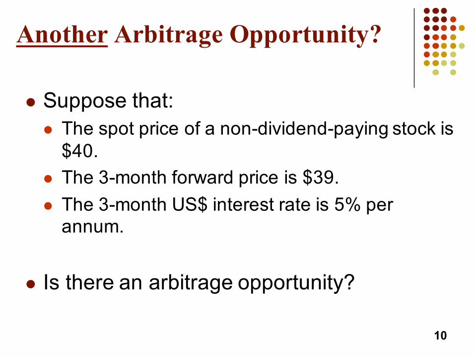
l Suppose that:l The spot price of a non-dividend-paying stock is
$40.l The 3-month forward price is $39.l The 3-month US$ interest rate is 5% per
annum.
l Is there an arbitrage opportunity?
10

Another Arbitrage Opportunity? Yes.
l Suppose that you short the stock, receive $40, and invest the $40 for 3 months at the risk-free rate.
l At the same time, you enter into a long futures contract.
l In 3 months, you must buy the stock (since you entered a contract to buy) and you pay $39 (the futures price).
l You receive from your investment $40x(1+0.05)(3/12) = $40.49
l You get to keep: $40.49 - $39 = $1.49 with no risk/investment.11
The Forward/Futures Price
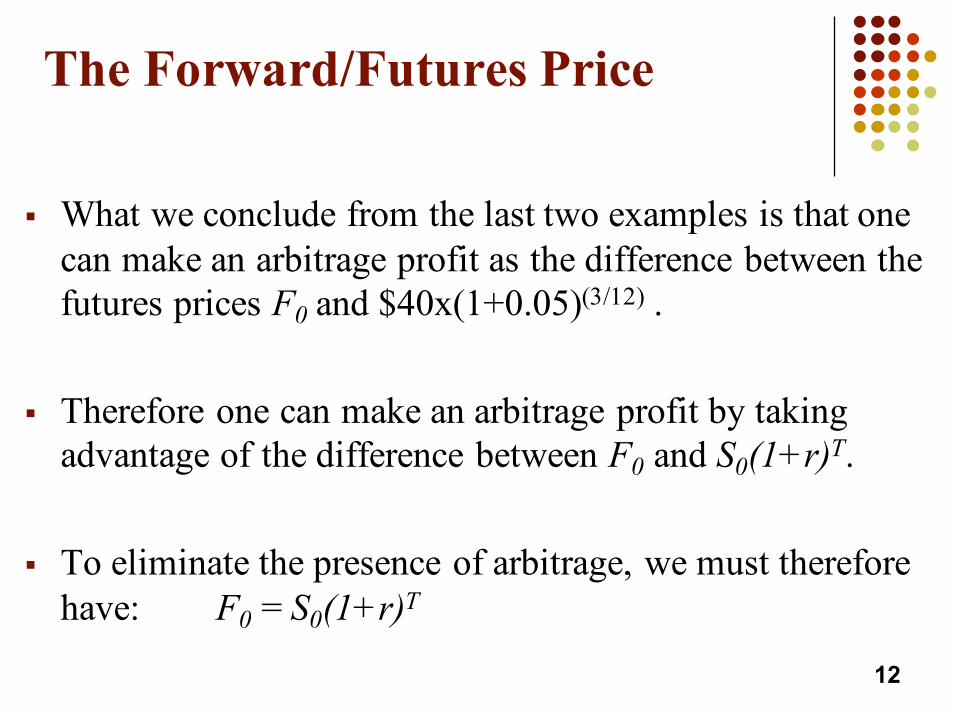
§ What we conclude from the last two examples is that one can make an arbitrage profit as the difference between the futures prices F0 and $40x(1+0.05)(3/12) .
§ Therefore one can make an arbitrage profit by taking advantage of the difference between F0 and S0(1+r)T.
§ To eliminate the presence of arbitrage, we must therefore have: F0 = S0(1+r)T
12

The Forward/Futures Price
l If the spot price of an investment asset is S0 and the futures price for a contract deliverable in T years is F0, then:
F0 = S0(1+r)T
where r is the T-year risk-free rate of interest.
l In our examples, S0 =40, T=0.25, and r=0.05 so that the no-arbitrage forward/futures price should be:
F0 = 40(1.05)0.25 =40.513

When using continuous compounding
§ F0 = S0erT
§ This equation relates the forward price and the spot price for any investment asset that provides no income and has no storage costs.
§ If short sales are not possible when the forward price is lower than the no-arbitrage price, the no-arbitrage formula (continuous or regular compounding) still works for an investment asset because investors who hold the asset (for investment purposes but not consumption) will sell it, invest the proceeds at the risk-free rate, and buy forward contracts.
§ If short sales are not possible when the forward price is higher than the no-arbitrage price, however, it’s a non-issue since the strategy would call for buying the stock (instead of short-selling it).
14

When an Investment Asset Provides a Known Dollar Income
l When an investment asset provides income with a present value of I during the life of the forward contract, we can generalize the previous formula as:
F0 = (S0 – I )erT
where I is the present value of the income during the life of the forward contract.
15

When an Investment Asset Provides a Known Dollar Income: Example
l Consider a 10-month forward contract on a $50 stock, with a continuous riskless rate of 8% per annum, and $0.75 dividends expected after 3 months, 6 months, and 9 months.
l The present value of the dividends, I, is given by:I = 0.75e-0.08x3/12 + 0.75e-0.08x6/12 + 0.75e-0.08x9/12 = 2.162
l The no-arbitrage forward price therefore must be:F0 = (50-2.162) e0.08x10/12 = $51.14
16

When an Investment Asset Provides a Known Yield
l Sometimes the underlying asset provides a known yield rather than a known cash income.
l The yield can be viewed as the income as a percentage of the asset price at the time it is paid.
l The no-arbitrage formula then becomes:F0 = S0 e(r–q )T
where q is the average yield during the life of the contract (expressed with continuous compounding)
17

When an Investment Asset Provides a Known Yield: Example
l Consider a 6-month forward contract on a $25 asset expected to produce a yield per annum of 3.96%, and a risk-free rate of 10%.
l The no-arbitrage price thus is: 25e(0.10-0.0396)x0.5 = $25.77
l Note that if you were not given the continuous yield directly but told that the income provided would be equal to 2% of the asset price during a 6-month period, you would need to convert from discrete to continuous:
l 2% in 6 months is equivalent to 3.96% per annum for 6 months with continuous compounding, because: 1+0.02 = eq(1/2)
l Backing out q as 2ln(1+0.02) we get q = 0.0396
18

Valuing a Forward Contract
l A forward contract is worth zero (except for bid-offer spread effects) when it is first negotiated.
l Banks are required to value all the contracts in their trading books each day, as later the contract may have a positive or negative value.
l Suppose that K is the delivery price and F0 is the forward price for a contract that would be negotiated today.
l The delivery is in T years from today and the continuously compounded risk-free rate is r.
19

Valuing a Forward Contract
l By considering the difference between a contract with delivery price K and a contract with delivery price F0 we can deduce that:
l The value, f, of a long forward contract isf = (F0 − K)e−rT or f = S0 − Ke−rT
l The value of a short forward contract is f = (K – F0 )e–rT or f = Ke−rT – S0
l If the asset provides a known income with present value I or a known yield q, for a long forward contract position, we have:
f = (F0 − K)e−rT or f = S0 − I − Ke−rT
or f = (F0 − K)e−rT or f = S0e−qT− Ke−rT
20
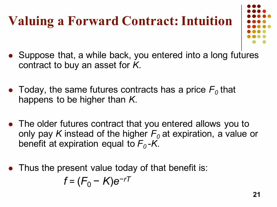
Valuing a Forward Contract: Intuition
l Suppose that, a while back, you entered into a long futures contract to buy an asset for K.
l Today, the same futures contracts has a price F0 that happens to be higher than K.
l The older futures contract that you entered allows you to only pay K instead of the higher F0 at expiration, a value or benefit at expiration equal to F0 -K.
l Thus the present value today of that benefit is: f = (F0 − K)e−rT
21

Valuing a Forward Contract: Intuition
l Suppose that, a while back, you entered into a short futures contract to sell an asset for K.
l Today, the same futures contracts has a price F0 that happens to be lower than K.
l The older futures contract that you entered allows you to receive K instead of the lower F0 at expiration, a value or benefit at expiration equal to K-F0.
l Thus the present value today of that benefit is: f = (K − F0)e−rT
22

Forward vs. Futures Prices
l When the maturity and asset price are the same, forward and futures prices are usually assumed to be equal. (Eurodollar futures are an exception, we will see this later).
l When interest rates are uncertain, futures and forward prices are, in theory, slightly different:l A strong positive correlation between interest rates and the asset price
implies the futures price is slightly higher than the forward price.l A strong negative correlation implies the reverse.
l For most practical purposes, however, we will assume that forward and futures prices are the same, equal to F0.
23

Stock Index (Page 116)
l Can be viewed as an investment asset paying a dividend yield.
l The futures price and spot price relationship is therefore
F0 = S0 e(r–q )T
where q is the dividend yield on the portfolio represented by the index during the life of the contract.
24

Stock Index (continued)
l For the formula to be true, it is important that the index represent an investable asset.
l In other words, changes in the index must correspond to changes in the value of a tradable portfolio.
l The Nikkei index viewed as a dollar number does not represent an investment asset, since Nikkei futures have a dollar value of 5 times the Nikkei.
25

Stock Index: Example
l Consider a 3-month futures contract on the S&P 500 index where the index yields 1% per annum.
l The current index value is 1,300 and the continuously compounded riskless rate is 5%.
l The futures price F0 must be: 1,300e(0.05-0.01)x0.25
l Thus F0 = $1,313.07
26

Index Arbitrage
l The arbitrage strategies are the same as when dealing with an individual security.
l When F0 > S0e(r-q)T an arbitrageur buys the stocks underlying the index and sells futures.
l When F0 < S0e(r-q)T an arbitrageur buys futures and shorts or sells the stocks underlying the index.
27

Index Arbitrage (continued)
l Index arbitrage involves simultaneous trades in the index futures contract and in many different stocks.
l Very often a computer is used to generate the trades: this is an example of program trading, the trading of many stocks simultaneously with a computer.
l Occasionally simultaneous trades are not possible and the theoretical no-arbitrage relationship between F0 and S0does not hold, as on October 19, 1987 (“Black Monday”).
28
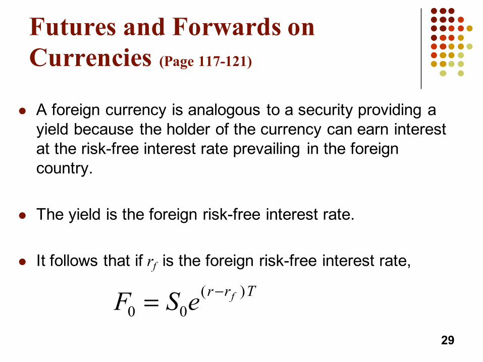
Futures and Forwards on Currencies (Page 117-121)
l A foreign currency is analogous to a security providing a yield because the holder of the currency can earn interest at the risk-free interest rate prevailing in the foreign country.
l The yield is the foreign risk-free interest rate.
l It follows that if rf is the foreign risk-free interest rate,
29
F S e r r Tf0 0= −( )

Explanation of the Relationship Between Spot and Forward
30
1000 units of foreign currency
(time zero)
1000S0 dollars at time zero
1000S0erT
dollars at time T
T
e Trf
time at currency foreign
of units 1000
TeF Trf
time at dollars1000 0

Arbitrage in Foreign Exchange Markets
31
l Suppose that the 2-year interest rates in Australia and the United States are 5% and 7%.
l The spot exchange rate is 0.62 USD per AUD.
l The 2-year forward exchange rate or price should be:0.62e(0.07-0.05)x2 = 0.6453
l What is the arbitrage if the forward rate is 0.63?l What is the arbitrage if the forward rate is 0.66?

Arbitrage in Foreign Exchange Markets
32
l If the forward rate is 0.63, the forward is underpriced (<0.6453).l Take a long position in the forward contract: an agreement to
buy AUD in 2 years at the rate of 0.63l Borrow 1,000 AUD today @ 5% per year, convert the amount
immediately to 1,000x0.62 = 620 USD and invest @ 7%.l Two years later, 620 USD grow to 620e0.07x2 = 713.17 USD.l Must repay the AUD loan: owe 1,000e0.05x2 = 1105.17 AUD.l Use the forward to buy 1105.17 AUD, costing 1105.17x0.63 or
696.26 USD and repay the loan balance of 1105.17 AUD.l Keep the difference 713.17 – 696.26 = 16.91 USD.

Arbitrage in Foreign Exchange Markets
33
l If the forward rate is 0.66, the forward is overpriced (>0.6453).l Take a short position in the forward contract: an agreement to sell
AUD in 2 years at the rate of 0.66l Invest in AUD today by first borrowing 1,000 USD @ 7% per year and
converting the amount immediately to 1,000/0.62 = 1,612.90 AUD. Therefore invest 1,612.90 AUD @ 5%.
l Two years later, 1,612.90 AUD grow to 1,612.90e0.05x2 = 1,782.53 AUD.
l Must repay the USD loan: owe 1,000e0.07x2 = 1,150.27 USD.l Use the forward to sell 1,782.53 AUD, giving you 1,782.53x0.66 or
1,176.47 USD and repay the loan balance of 1,150.27 USD.l Keep the difference 1,176.47 – 1,150.27 = 26.20 USD.

Futures on Commodities that are Investment Assets (Gold, Silver, …)
l With commodity futures, one has to take into account possible storage costs of the commodity (because implementing an arbitrage strategy might imply the buying –and thus the storing – of the commodity).
l Storage costs can be viewed as negative income or yield.l Letting u be the storage cost per unit time as a percent of
the asset value, we have:F0 = S0 e(r+u )T
l Alternatively, letting U be the present value of the storage costs, we have:
F0 = (S0+U )erT
34
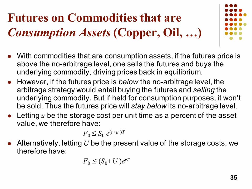
Futures on Commodities that are Consumption Assets (Copper, Oil, …)
l With commodities that are consumption assets, if the futures price is above the no-arbitrage level, one sells the futures and buys the underlying commodity, driving prices back in equilibrium.
l However, if the futures price is below the no-arbitrage level, the arbitrage strategy would entail buying the futures and selling the underlying commodity. But if held for consumption purposes, it won’t be sold. Thus the futures price will stay below its no-arbitrage level.
l Letting u be the storage cost per unit time as a percent of the asset value, we therefore have:
F0 ≤ S0 e(r+u )T
l Alternatively, letting U be the present value of the storage costs, we therefore have:
F0 ≤ (S0+U )erT
35

Convenience Yield
l With consumption asset commodities we thus have:F0 ≤ S0 e(r+u )T
l Therefore the difference between F0 and S0 e(r+u )T can be viewed as reflecting the convenience of holding the physical consumption asset (rather than the futures contract on it).
l So if we let y be the parameter that will equate the two:l we then must have: F0 eyT= S0 e(r+u )T
l y is referred to as the convenience yield, and we have:F0 = S0 e(r+u -y)T
36

The Cost of Carry (Page 124)
l The cost of carry, c, is the interest cost - income earned + storage costs, so c = r – q + u
l For an investment asset F0 = S0ecT
l For a consumption asset F0 ≤ S0ecT
l The convenience yield on the consumption asset, y, is defined so that
F0 = S0 e(c–y )T
37

Futures Prices & Expected Future Spot Pricesl Suppose k is the expected rate of return required by
investors on an asset.
l We can invest F0e–r T at the risk-free rate and enter into a long futures contract to create a cash inflow of ST at maturity.
l This shows that:
38
( )0 0( ) or ( )rT kT r k T
T TF e E S e F E S e− − −= =

Futures Prices & Future Spot Prices
39
No Systematic Risk (β=0) k = r F0 = E(ST)Positive Systematic Risk (β>0) k > r F0 < E(ST)Negative Systematic Risk (β<0) k < r F0 > E(ST)
Positive systematic risk: stock indices (Normal Backwardation)
Negative systematic risk: gold (at least for some periods, Contango)
However, the terms backwardation and contango are also often used to describe whether the futures price is below or above the spot price S0.


![Determination of Forward and Futures Pricesdupoyetb/Financial_Risk_Mgt/lectures/Ch05.pdfExample l The profitfrom shorting is 100 x [ 100 – 3 – 90 ] = $700. l Note that the dividend](https://static.fdocuments.in/doc/165x107/612982281a6b924170218e0d/determination-of-forward-and-futures-prices-dupoyetbfinancialriskmgtlecturesch05pdf.jpg)