Market Timing with Aggregate and Idiosyncratic Stock Volatilities
From Currency Volatilities to Global Equity Correlations
Brice Dupoyet *
Florida International University, College of Business Administration
Ali M. Parhizgari
Florida International University, College of Business Administration
Antonio Figueiredo
Nova Southeastern University, Huizenga College of Business & Entrepreneurship
Abstract
We derive and empirically test a theoretical link between exchange rate volatility and global equity
correlations. Starting with option-implied currency volatilities, we use global capital flows, international
parity, the Taylor rule, and some simplifying assumptions to theoretically link foreign exchange options-
implied volatilities and future global equity correlations. Using daily data from January 1999 to June 2015,
we test our theory and find that exchange rate implied volatilities - coupled with one-period ex-post
correlations - more accurately predict subsequent equity market correlations than any other model. Our
findings have implications for portfolio diversification, forecast of overall equity portfolio volatility, and
portfolio optimization.
Keywords: Exchange Rate, Volatility, International Equity, Correlations
JEL Classification Codes: C32, E44, E47, G15.
* Corresponding Author:
Brice Dupoyet, Florida International University
College of Business, RB 229A
11200 Southwest 8th Street, Miami, FL 33199
Tel: (305) 348 3328, Fax: (305) 348 4245
E-mail: [email protected]
1. Introduction
Volatility and correlation forecasts are significant components of asset pricing and financial risk
management. Prior literature on the measurement, modeling, and forecasting of volatility abounds, with
Poon and Granger (2003) providing a comprehensive coverage of such studies. However, although
volatility and correlations play a joint central role in the behavior of any portfolio, little serious effort has
yet been made to link these two concepts together. We posit and test a parsimonious theoretical model to
establish this link. Further, we show how this model could be used to forecast correlations among global
equity markets. More specifically, we consider two seemingly unrelated concepts - exchange rates and
equity correlations - side-by-side. We establish the linkage between international equity markets’
correlation levels and the volatility of the exchange rates pertinent to these markets. As a driving measure,
we focus on forward-looking option-implied measures of currency exchange rate volatilities to capture
ex-ante measures of correlations among the associated international equity markets.
The benefits of forecasting future correlation levels with reasonable accuracy are obvious.
Correlations are the driver of diversification and a key measure in any type of portfolio optimization
process since they help determine the optimal portfolio weights. Forecasting a constant value may be a
simple task, but correlations may not be constant. Equity markets correlations and volatilities have been
shown to be time varying (Longin and Solnik, 1995 and 2001), yet the main determinants of these time
variations are not fully known and remain an active area of research. Thus, uncovering new insights into
the dynamics of the drivers of global equity markets correlations is of great interest. We show that such
new findings can be employed to reduce correlation forecast errors. We also compare our approach with
the “naïve” forecast often found in practice where future equity correlation levels among global markets
are assumed to be stable and thus simply estimated from the most recent sample period. Reducing
correlation forecast errors should then result in more appropriate portfolio weights and thus in higher

Sharpe ratios. Our study greatly expands on the suggestions by Della Corte, Sarno, and Tsiakas (2012)
that volatility and correlation timing is possible and clearly beneficial in international asset allocation.
On the theoretical front, we contribute to the current literature by positing a unified framework
linking economic fundamentals with correlations among international equity markets. A noteworthy
aspect of this framework is that the posited link between foreign exchange volatility and equity
correlations is built around well-established theoretical constructs. In this regard, we face three distinctive
challenges. First, we link the monetary side of the economy with its real side counterpart. Second, we link
the monetary side of the economy to currency volatility as well as the real side of the economy to volatility
in the equity markets. Finally, we establish correlations among these two groups of volatilities.
Prior research relevant to the scope of this paper is seldom attempted. While exchange rates and
equity markets are amply covered separately, they are rarely brought together in a theoretical framework.
For instance, Evan’s (2011) pioneering detailed work is exclusively on the dynamics of exchange rate.
Equity markets simply do not fall within the scope of his work, so they are obviously not addressed. Evan’s
(2011) comprehensive work on exchange rate dynamics encompasses diverse modeling approaches such
as macro models, microstructure models, micro-based macro models, and monetary models. The
theoretical link between exchange rate volatility and equity correlations presented in our study originates
from the assumption of a monetary-based exchange rate model drawn from Evan (2011), or more
specifically, a Taylor rule based model. On equity markets, there is a significant number of contributions,
but for the most part they are shy of exchange rates (e.g. Pukthuanthong and Roll, 2009; Veronesi, 1999;
Cai et al., 2009). Regarding the blending of the two together, one of the very few prior related studies that
attempts to provide some theoretical explanation for increased equity correlations during economic
downturns proposes to use an intertemporal rational expectations model wherein uncertainty about the
state of the global economy is attributed to higher international equity correlations during economic
downturns (e.g. Veronesi, 1999; Ribeiro and Veronesi, 2002). Under the assumption that uncertainty about
the U.S. economy also implies uncertainty about the global economy, and that equity investors would
require to be compensated for this increased risk, there is some theoretical evidence that international
equity markets in countries whose economies are sensitive to the global business cycle would decline
somewhat in unison during periods of high uncertainty, thus increasing correlation among equity markets.
There is ample empirical evidence supporting this phenomenon during the 2008-2009 financial crisis (e.g.
Bekaert et al., 2014; Briere et al., 2012; Samarakoon, 2011). However, there are also some differing
opinions on the matter. For instance, Forbes and Rigobon (2002) refute the notion of contagion during the
1997 Asian crisis and the U.S. stock market crash of 1987 by showing no increase in unconditional
correlation coefficients during these periods. Instead, they argue that correlations are conditional on
market volatility and that this ‘interdependence’ is always present, not only during periods of crisis.
On the empirical side, we test our proposed theory by examining the relation between option-
implied volatility in foreign exchange markets and future international equity market correlations for 11
countries and the pan-European STOXX index. Our findings support our posited theory on the existence
of a relation between option-implied exchange rate volatility and subsequent correlations among the equity
markets. We exploit the dynamics of this relation to provide ex-ante forecasts of future correlations.
Additionally, we compare the relation between foreign exchange volatility and equity correlations with
that of equity volatility and equity correlations. This comparison yields further insights into the factors
that drive international equity correlations.
Some intuition into our two seemingly unrelated concepts of correlations and exchange rates is
necessary. Heretofore, several studies such as Roll (1998) and Longin and Solnik (1995) have
demonstrated that international markets tend to move together more when equity volatility is high. Longin
and Solnik (2001) also find that such correlations are more specifically related to bearish market trends
than to volatility directly. However, high volatility and declining markets tend to go hand in hand, as
evidenced by a widely observed negative relation between the CBOE’s VIX (Chicago Board Options
Exchange’s established indicator of market volatility) and the S&P 500 index. The empirical evidence
linking equity volatility – and/or the VIX as its proxy – to equity correlation is therefore compelling, but
it lacks solid theoretical support. While volatility in the world’s largest equity market and economy is
likely to affect most equity markets and economies around the globe, the strength of its impact is likely to
depend on the extent of bilateral trade and economic interdependence. The theory and measurement of
this impact, however, are lacking. For instance, the VIX measure does not capture any of these dynamics.
Given that foreign exchange rates are a major factor in bilateral trade as argued by Forbes and Chinn
(2004), we hypothesize that option-implied foreign exchange volatility can better reflect such dynamics
between any given two countries, and is thus a more effective predictor of equity correlations than the
VIX.
To the best of our knowledge, there is no consensus in the financial economics literature regarding
the link between economic fundamentals and correlations among international equity markets. This is
somewhat surprising given that there are several, though segmented, proposed theoretical economic
models and empirical studies demonstrating a relation between equity correlations and economic
indicators such as business cycles, inflation, and economic output (e.g. Erb et al., 1994; Longin and Solnik,
1995; Moskowitz, 2003; Forbes and Chinn, 2004; Graham et al., 2012; Cai et al., 2009). There is also
another vein of analyses cutting in the middle or completely departing from the mainstream. This group
argues that such relation - if it exists - is either not significant enough or not stable over time (e.g. King et
al., 1994; Ammer and Mei, 1996; Kizys and Pierdzioch, 2006). In light of these previous studies, the
importance and relevance of establishing a rigorous testable theoretical link is therefore evident.

The novelty of our approach and its contribution to the current literature is better appraised through
some comparisons with the pioneering studies of Forbes and Chinn (2004), Aslanidis and Casas (2013)
and Bodart and Reding (1999). These researchers consider, respectively, bilateral trade and portfolios of
equities and currencies as a way to reach correlations. They thus provide, though partially, some isolated
segments of the theory we seek to establish. While we find these studies helpful, there are a few other
contributions that have not been much encouraging to our cause. For example, contrary to our findings
that equity correlations are positively related to implied exchange rate volatility, Bodart and Reding (1999)
find that “an increase in exchange rate volatility is accompanied by a decline in international correlations
between bond and, to a lesser extent, stock markets.” Obviously, there are important and clear distinctions
between our study and Bodard and Reding’s (1999). Yet, this example attests the unsettled positions, both
theoretically and empirically, on the topic we have chosen to address. Arguably, BR’s study is mainly on
bonds, void of any measures of currency volatilities, and limited to a comparison between countries within
and outside the EU Monetary System. Our study, on the other hand, examines how the equity correlation
between a given pair of international equity markets is related to the volatility of the pertinent exchange
rate for these two markets. Specifically, our analysis utilizes a daily market-driven measure of implied
volatility for exchange rates.
In light of the above points, it is evident that the breadth and scope of the prior contributions are
highly diverse, that a clear consensus is lacking, and that a well-grounded and empirically tested approach
to establish the link between currency volatilities and global equity correlations is warranted. This is, as
stated earlier, the aim of this paper.

2. Theoretical Model
Given that there is no widely accepted theory linking exchange rate volatility to international
equity market correlations, we first consider a few intuition-based relations that draw upon asset-pricing
models and parity fundamentals. We then derive a generalized theoretical framework and subsequently
test it empirically. For simplicity, we start with a two-market (country) two-currency situation. We denote
the two countries by “EUR” and “US”, with “EUR” representing any country in the Euro zone. Under
standard Black-Scholes distributional assumptions, the dollar/euro spot exchange rate follows:
𝑆𝑡 = 𝑆0exp{(𝑟𝐸𝑈𝑅 − 𝑟𝑈𝑆)𝑡 − 𝜎2𝑡 2⁄ + 𝜎𝑊𝑡} (1)
where St is the spot exchange rate at time t expressed in euros per dollar, S0 is the spot exchange rate at
time 0, 𝑟𝑈𝑆 and 𝑟𝐸𝑈𝑅 are the respective dollar-denominated and euro-denominated risk-free rates for the
pertinent period from time 0 to time t, σ is the volatility of the exchange rate between time 0 and t, and Wt
is a Wiener process. The above expression is the process forming the basis for currency option pricing
under Black-Scholes.
On the surface, relation (1) is seemingly unrelated to the real side of the economy, i.e., to equity
markets1. Upon further scrutiny, we will demonstrate that 𝑆𝑡 or its volatility is indeed related to the real
side of the global economy and thereby to the correlations among its components. To facilitate the
derivations that follow, Figure 1 provides a schematic flowchart showing the steps in our approach from
currency volatility to global equity correlations. Starting with a Taylor-rule based model of real exchange
rates and applying the basic concept of variance of a linear combination of random variables, we show
that high foreign exchange volatility implies high correlation between the two pertinent countries’
inflation and output gap differentials. This in turn implies that there is also a high correlation between
1 For comparison, see Zellner (1962).
these countries’ risk-free rates and output gap differentials given the relation between inflation and interest
rates based on the Fisher rule. Finally, assuming that broad equity markets are a discounted value of the
aggregate countries’ cash payouts to investors and that such cash payouts are related to the countries’
outputs, we demonstrate that a high correlation between two countries’ risk-free rates and output gap
differentials also implies high equity market correlations.
The differential interest rate term (𝑟𝐸𝑈𝑅 − 𝑟𝑈𝑆)in equation (1) is the key element to our
derivations. For spot exchange rate quotes at time t, we assume an equilibrium price based on a micro-
based macro model for the dollar-euro spot rate that is a simplified version of the model proposed by
Evans and Lyons (2008). The original model, along with several other exchange rate models, are described
in detail in Evans (2011). Our simplified version of the model has the form:
𝑆𝑡 = 𝔼𝑡𝑆𝑡+1+(𝑟𝐸𝑈𝑅,𝑡 − 𝑟𝑈𝑆,𝑡) (2)
where 𝔼𝑡 denotes the expectation of the market based upon the information available at time t, 𝑟𝑈𝑆 and
𝑟𝐸𝑈𝑅 are as defined earlier and are now analogous to risk-free short-term dollar and euro rates for a given
period. Moving forward one period, equation (2) becomes:
𝔼𝑡𝑆𝑡+1 = 𝔼𝑡𝑆𝑡+2+𝔼𝑡[𝑟𝐸𝑈𝑅,𝑡+1 − 𝑟𝑈𝑆,𝑡+1] (3)
In equation (2), the risk-free rates at time t are observed, while in equation (3) they are based on
equilibrium market expectations of central banks’ actions (for instance, the Federal Reserve and the
European Central Bank) in response to changes in the macro economy. To expand relation (3), we resort
to the Taylor rule. Taylor rule-based models for interest rates assume that central banks set nominal rates
based on the divergence of inflation from inflation targets and the divergence of GDP from potential GDP.
Specifically, employing a modified version of the real exchange rate definition based on Evans and Lyons
(2011), interest rate expectations are set according to:
𝔼𝑡[𝑟𝐸𝑈𝑅,𝑡+1 − 𝑟𝑈𝑆,𝑡+1] = (1 + 𝜆𝜋)𝔼𝑡[π𝐸𝑈𝑅,𝑡+1+𝑖 − π𝑈𝑆,𝑡+1+𝑖] + 𝜆𝑦𝔼𝑡[𝑦𝐸𝑈𝑅,𝑡+1 −
𝑦𝑈𝑆,𝑡+1] − 𝜆𝜉𝔼𝑡𝜉𝑡+1
(4)
where i > 0, π𝐸𝑈𝑅,𝑡+1+𝑖 − π𝑈𝑆,𝑡+1+𝑖 represents the future difference between inflation in the Euro zone
and the U.S., 𝑦𝐸𝑈𝑅,𝑡+1 − 𝑦𝑈𝑆,𝑡+1 represents the future difference in log output (GDP) between the Euro
zone and the U.S., 𝜉𝑡 ≡𝑠𝑡+ 𝑝𝐸𝑈𝑅,𝑡 − 𝑝𝑈𝑆,𝑡 is the real exchange rate (𝑝𝐸𝑈𝑅,𝑡 and 𝑝𝑈𝑆,𝑡 are log price indices),
and 𝜆𝜋, 𝜆𝑦 , 𝜆𝜉 are positive coefficients. The derivation of relation (4) is provided in Appendix A. Relation
(4) implies that market participants expect the euro-dollar rate differential to be higher when the
corresponding future inflation differential is higher, when the output gap is wider, or when the real
exchange rate declines. The first two implications suggest that central banks should raise short-term
interest rates when inflation and output gap rise, a widely-held view. The last implication suggests that
deviations from purchasing power parity levels have some impact on central banks’ rate setting decisions.
Our model, as is the case in the original Evans and Lyons (2008) model, does not require that central
banks follow a known recipe for setting rates such as the Taylor rule, but simply that market expectations
of future rates are driven by market expectations of inflation and output macro variables. The output gap
is essentially a substitute for a differential in productivity measures, which in turn can easily be linked to
equity market returns2. Irrespectively of these details, our intent to link 𝑆𝑡 with the real side of the economy
is well in place in light of equations (1) through (4).
Substituting the value for rate expectations from equation (4) into equation (3) and iterating
forward yields:
𝔼𝑡𝑆𝑡+1 = 𝔼𝑡∑𝛾𝑖
∞
𝑖=1
𝑓𝑡+1 (5)
2 See, for instance, Parhizgari and Aburachis (2004).
where it is assumed that 𝔼𝑡 limi→∞
𝛾𝑖 𝑠𝑡+𝑖 = 0, 𝛾 = 1 (1 + 𝜆𝜀) < 1⁄ , and
𝑓𝑡 = (1 + 𝜆𝜋)[𝜋𝐸𝑈𝑅,𝑡+1 − π𝑈𝑆,𝑡+1] +𝜆𝑦[𝑦𝐸𝑈𝑅,𝑡 − 𝑦𝑈𝑆,𝑡] + (
1 − 𝛾
𝛾) [𝑝𝑈𝑆,𝑡 − 𝑝𝐸𝑈𝑅,𝑡] (6)
A more detailed derivation is provided in Appendix B. Equation (5) represents the market
expectations for exchange rates for the next period in terms of the market expectations for macroeconomic
fundamentals denoted by 𝑓𝑡. Substituting the results of equation (5) into equation (2) we have:
𝑆𝑡 = (𝑟𝐸𝑈𝑅,𝑡 − 𝑟𝑈𝑆,𝑡) + 𝔼𝑡∑𝛾𝑖
∞
𝑖=1
𝑓𝑡+1 (7)
Defining variation in exchange rate as Δ𝑆𝑡+1 = 𝔼𝑡Δ𝑆𝑡+1 + 𝑆𝑡+1 − 𝔼𝑡𝑆𝑡+1, and combining it with
equation (2) yields
Δ𝑆𝑡+1 = (𝑟𝑈𝑆,𝑡 − 𝑟𝐸𝑈𝑅,𝑡) + 𝑆𝑡+1 − 𝔼𝑡𝑆𝑡+1 (8)
Equations (2) through (8) draw heavily upon Evans (2011), save some minor modifications.
Considering equations (7) and (8) together, variations in exchange rates over short periods are primarily
driven by revisions of future expectations of the macroeconomic variables, or the asset side of the
economy. This can also be inferred by taking the variance on both sides of equation (5). Consequently,
exchange rate volatility is driven by the volatility of future expectations of the macroeconomic variables.
Based on the definition of the macro fundamentals 𝑓𝑡 in relation (6), exchange rate volatility is a
function of the variance in the difference of macroeconomic variables in two countries and the correlation
among them, implying that high volatility in exchange rates are associated with high correlation among
the difference in macroeconomic variables. This arises because of the well-known identity
𝑉𝑎𝑟(𝑎𝑋 + 𝑏𝑌) = 𝑎2𝜎𝑥2 +𝑏2𝜎𝑦
2 + 2𝑎𝑏𝜌𝑥,𝑦𝜎𝑥𝜎𝑦 from which it is clear that given a certain value of 𝜎𝑥,
𝑉𝑎𝑟(𝑎𝑋 + 𝑏𝑌) will be maximized when 𝜌𝑥,𝑦 = 1 since 𝜎𝑥 ≥ 0, 𝜎𝑦 ≥ 0, 𝑎𝑛𝑑 − 1 ≤ 𝜌𝑥,𝑦 ≤ 1.Therefore,
taking into account the first two terms of equation (6), we can conclude that volatility of dollar/euro
exchange rate will be maximized when the correlation between the inflation differential [𝜋𝐸𝑈𝑅,𝑡+1 −
π𝑈𝑆,𝑡+1] and the log output gaps [𝑦𝐸𝑈𝑅,𝑡 − 𝑦𝑈𝑆,𝑡] is 1. In this maximization state, the inflation differential
is a linear combination of the log output gaps and thus can be expressed as:
𝜋𝐸𝑈𝑅,𝑡+1 − π𝑈𝑆,𝑡+1 = 𝐾1,𝑡[𝑦𝐸𝑈𝑅,𝑡 − 𝑦𝑈𝑆,𝑡] + 𝐾2,𝑡 (9)
where 𝐾1,𝑡 and 𝐾2,𝑡 are constants, and where 𝑦𝑈𝑆,𝑡 and 𝑦𝐸𝑈𝑅,𝑡represent the log of the real output of the
U.S. and the Euro zone, respectively.
Equation (9) also implies that
𝑟𝐸𝑈𝑅,𝑡 − r𝑈𝑆,𝑡 = 𝐾1,𝑡[𝑦𝐸𝑈𝑅,𝑡 − 𝑦𝑈𝑆,𝑡] + 𝐾2,𝑡 (10)
since the Fisher Effect holds that an increase (decrease) in the expected inflation rate in a country will
cause a proportional increase (decrease) in the interest rate of that country. After a few steps shown in
Appendix C, equation (10) can be expressed as:
𝐾0,𝑡
𝑌𝐸𝑈𝑅,𝑡
𝑒𝑟𝐸𝑈𝑅,𝑡 𝐾1,𝑡⁄ =𝑌𝑈𝑆,𝑡
𝑒𝑟𝑈𝑆,𝑡 𝐾1,𝑡⁄ (11)
where 𝑌𝑈𝑆,𝑡 represents the real output for the U.S., 𝐾0,𝑡 = 𝑒𝑥𝑝(𝐾2,𝑡
𝐾1,𝑡), and analogously 𝑌𝐸𝑈𝑅,𝑡 represents
the real output for the Euro zone. Therefore, in the spot rate volatility maximization state, equation (9)
states that the correlation between the inflation differential in the U.S. and the Euro zone and the output
gap between the countries is maximized at 1. This also implies that the correlation between the discounted
real output of the two countries is also maximized at 1 as shown in equation (11).
Under the risk-neutral probability measure, the broad equity market value for the U.S., denoted as
𝑀𝑈𝑆, is given by:
𝔼𝑡𝑀𝑈𝑆,𝑡 = ∫ 𝑒−𝑟𝑈𝑆(𝜏−𝑡)
∞
𝑡
𝐷𝜏𝑑𝜏 (12)
where 𝐷𝜏 represents an aggregate cash payout to investors that is linked to the country’s output. The broad
equity market value for the Euro zone is defined analogously. If the cash payout to investors in each
country is a proportion of the real output of that country, we can then conclude that when the volatility of
the spot rate between the two countries approaches a maximum, the correlation between the discounted
market values for the two countries should also approach its maximum of 1. Assuming that all (currency,
equity, and option) market participants have the same access to information regarding interest rates and
the state of the macro economy, the model described in this section provides a theoretical justification for
the hypothesis that implied volatility in currency option prices is positively related to equity market
correlations over the life of the option.
So far, we have shown that under some plausible assumptions there is a theoretical justification
for equity correlations between two countries to be elevated when the volatility of the exchange rate
between the two countries’ currencies is high. Assuming that option-implied foreign exchange rate
volatility is a good predictor of subsequent observed foreign exchange rate volatility, it should then follow
that option implied exchange rate volatility would be a contributing factor in the forecast of subsequent
equity correlations. At the empirical level, further modifications and fine-tuning of the above relations
become necessary; these will be discussed in Section 4.
As mentioned earlier, the forecast of correlations is a key ingredient in the calculation of the
optimal portfolio’s weights. In the case of a global portfolio comprised of broad exposure to equity
markets in various countries, we contend that the forecast of future correlations between any country pair
would be more accurate if the pertinent option implied exchange rate volatility were a factor in such
forecast. Nonetheless, the theoretical justification we have put forth suggests that this is especially true
when the exchange rate volatility is elevated. Therefore, our empirical work centers on evaluating the
following relation:
𝐶𝑜𝑟𝑟𝑋𝑌𝑡,𝑡+3 = 𝐶𝑜𝑟𝑟𝑋𝑌𝑡−3,𝑡 + 𝐹𝑋𝐼𝑉𝑡 + 𝐹𝑋𝑑𝑢𝑚𝑚𝑦𝑡 +𝜀𝑡 (13)
where 𝐶𝑜𝑟𝑟𝑋𝑌𝑡,𝑡+3 corresponds to the pairwise correlation over the three-month ahead period starting at
time t, 𝐶𝑜𝑟𝑟𝑋𝑌𝑡−3,𝑡 represents the pairwise correlation over the three-month period preceding time t,
𝐹𝑋𝐼𝑉𝑡 is the pertinent foreign exchange option implied volatility at time t, and 𝐹𝑋𝑑𝑢𝑚𝑚𝑦𝑡 is the
interaction between this implied volatility and a dummy variable set to 1 (zero) to indicate a period of
high (low) volatility. The threshold value used to set this dummy variable is based on historical patterns
of volatility levels.
Taking into consideration previous studies’ findings that demonstrate the relation between equity
volatility and equity correlations (e.g. Longin and Solnik, 2001; Connolly et al., 2007; Cai et al., 2009),
we also consider the following relation:
𝐶𝑜𝑟𝑟𝑋𝑌𝑡,𝑡+3 = 𝐶𝑜𝑟𝑟𝑋𝑌𝑡−3,𝑡 + 𝐹𝑋𝐼𝑉𝑡 + 𝐹𝑋𝑑𝑢𝑚𝑚𝑦𝑡 + 𝑉𝑖𝑥𝑑𝑢𝑚𝑚𝑦𝑡 +𝜀𝑡 (14)
where 𝑉𝑖𝑥𝑑𝑢𝑚𝑚𝑦𝑡 is the interaction between the value of the VIX at time t and a dummy variable set to
1 (zero) to indicate a period of high (low) volatility when the VIX index is above (below) 25 at time t. All
other variables are as defined in equation (13). Once again, the threshold value used to set the
𝑉𝑖𝑥𝑑𝑢𝑚𝑚𝑦𝑡 variable is based on the VIX levels’ historical patterns. Empirically evaluating equation
(14) is necessary to determine whether the inclusion of exchange rate volatility in the forecast yields any
incremental benefits when equity volatility is also used as a factor.
3. Data and Sources
Our primary data range from January 1st, 1999 to June 30th, 2015 and include the daily values of
eight foreign exchange rates, the S&P 500 index 30-day implied volatility VIX, the one-month, three-
months, and one-year at-the-money foreign exchange rate options implied volatilities, and finally the
returns of 11 international single-country equity indices and the pan-European STOXX index. The sample
period’s starting date coincides with the introduction of the Euro currency.
The option-implied volatilities reflecting the market’s expected future volatility of the respective
currencies from the present (time t) to maturity for the eight exchange rates are obtained directly from
Bloomberg, using options with three months to maturity. The foreign currencies used are: the Euro, the
British Pound, the Japanese Yen, the Swiss Franc, the Canadian Dollar, the Australian Dollar, the Mexican
Peso, and the Brazilian Real. In order to compute correlations among international equity markets in a
common currency, we employ the Datastream U.S. dollar denominated daily values for the equity indices
included in our study. In total, we examine the returns and pairwise correlations of 12 equity indices. Four
of these markets (plus the pan-European STOXX index) are markets where the Euro is the official
currency. The other seven of these markets correspond to markets wherein each of the other foreign
currencies in our sample is the official currency. The U.S. is the benchmark market in our sample used for
the correlations calculations. Specifically, we use the main equity index in the United States (S&P 500),
Canada (S&P/TSX composite), United Kingdom (FTSE 100), Australia (S&P/ASX 300), Germany (DAX
30), France (CAC-40), Switzerland (SMI), Spain (IBEX 35), Italy (FTSE MIB), Japan (NIKKEI 225),
Mexico (IPC), and Brazil (BOVESPA) as proxies for the broad equity markets in these countries.
4. Empirical Applications and Results
At the empirical level, applications of equations (8) through (12) in conjunction with equation (1)
require some computations and substitutions. Very briefly, these include the following steps:
1. Identifying the employed volatility measures
2. Linking implied volatility with a forecast of the one-period ahead realized volatility
3. Measuring equity correlations
4. Linking currency volatilities of steps 1 and 2 with equity correlations of step 3 via an
autoregressive error correction model3 (See Appendix D for details).
Obviously, steps 1 through 4 above do not automatically correspond to any of the relations
expressed in (8) through (12). This ‘seemingly unrelated’ reference will be clarified as we move through
each step and as we identify and assign various components to their underlying variables in equations (8)
through (12).
4.1 Identification of employed volatility measures
As implied volatility measures, we employ Bloomberg’s exchange rate implied volatility for one
month, three months, and one year. Realized exchange rate volatility is calculated via two approaches:
variance of exchange rates over a given period (classical method), and by applying the Garman and Klass
(1980) methodology. The former is given by:
𝜎𝑆�̂�2 =
1
𝑁 − 1∑(𝐹𝑋_𝑅𝐸𝑇𝑡 − 𝐹𝑋_𝑅𝐸𝑇)
2𝑁
𝑡=1
(15)
3 We correct for autocorrelation in the error term by modeling the random error term with an autoregressive feature. It is not
the same as the error correction model of Engle and Granger (1987).

where 𝐹𝑋_𝑅𝐸𝑇𝑡 represents the daily change in the foreign exchange rate on day t calculated using first
differences, and 𝐹𝑋_𝑅𝐸𝑇 is the mean foreign exchange daily change over the measured period. The
standard deviation is simply the square root of the calculated variance. We then annualize the daily
standard deviation by multiplying it by the square root of 365. We perform this calculation for each of the
eight foreign exchange rates used in our study and over each day in our data sample, measuring realized
volatility over one-, three-, and twelve-months ahead rolling periods.
In the second method, following Garman and Klass (1980), we use open, close, high, and low daily
values to measure volatility of Δ𝑆𝑡. It is shown that this measure is about eight times more efficient than
a simpler measure that uses close-to-close daily values4. Specifically, we employ the reduced-form
estimator that yields virtually the same level of efficiency as the full-form estimator. The difference is that
the reduced-form estimator specification has marginally different coefficients and excludes cross-product
terms. Under this methodology, we calculate realized volatility levels as the average of the daily
volatilities during the period, with the volatility on a given day t being:
𝜎𝑆𝑡2 =
1
2[ln(𝐻𝑖𝑔ℎ) − ln(𝐿𝑜𝑤)]2 − [2 ln 2 − 1][ln(𝑂𝑝𝑒𝑛) − ln(𝐶𝑙𝑜𝑠𝑒)]2 (16)
where High, Low, Open, and Close represent the daily high, low, open, and close exchange rates. We
perform this calculation for each of the eight foreign exchange rates and for each day in our sample,
measuring realized volatility over rolling periods of one-, three-, and twelve-months ahead. Table 1 reports
the summary statistics for the currencies’ volatility levels and the VIX.
4 See Garman and Klass (1980), p. 74.
4.2 Linking implied volatility to a forecast of a one-period ahead realized volatility
Using the above computed measures of realized volatility, we are now able to examine the efficacy
of Bloomberg’s option implied foreign exchange rate volatility measures5 as a forecast of actual currency
volatilities. Within the framework we have adopted, we evaluate the forecasts for one-, three-, and twelve-
month horizons using both afore-calculated volatility measures. To evaluate the results, we compute the
mean absolute percentage error (MAPE) for each forecast and report them in Table 2. An analysis of the
results lead to the following general conclusions: Bloomberg’s option implied currency volatilities are
good predictors of actual subsequent currency volatility as their mean absolute percentage errors are lower
than 0.5% in all cases using the Garman-Klass method except for the Brazilian real. Additionally, shorter
horizon forecasts are more accurate, and forecast errors are lower for the major currencies than for
emerging market currencies. These observations are consistent with the fact that options of major
currencies and of shorter maturities tend to exhibit greater liquidity.
4.3 Measuring equity correlations
This section focuses on equations (9) and (11) and the correlation between the real sides of two
economies. First, it is assumed that the real side of an economy may be represented by the assets or the
equity markets’ side of that country. Second, to address the notion that correlations increase in times of
higher volatility, we designate September 2008 to August 2009 as the most recent notable period of high
volatility and focus on it as a separate time period. We then calculate unconditional correlations among
the 12 equity markets for both the full sample and the shorter period of crisis, and report the results in
5 These measures are readily available from Bloomberg. See Section 3 on data and sources.
Table 3.6 Economic ties appear to be an important factor in determining the correlation among equity
markets. For example, Panel A in Table 3 shows that the U.K.’s equity market correlation coefficient with
other European markets range from 0.72 to 0.82 versus 0.27 to 0.58 for non-European markets in our
sample universe. Another notable fact is the across-the-board significant increase in correlation during the
2008-2009 crisis period. For instance, over the entire sample period the correlation coefficient for Japan’s
equity market with any other market in our sample universe ranged from 0.19 to 0.44. During the crisis
period included in Panel B the corresponding range is from 0.51 to 0.66. Correlation coefficients among
the European equity markets during the crisis period reported in Panel B of Table 3 rose to as high as 0.96
reflecting their strong economic ties.
Additionally, considering the monetary components of equations (9) and (11), we categorize the
equity markets based on the volatility of the currency markets. Focusing on the historical implied foreign
exchange volatilities of three major currencies (Euro, British Pound, and Swiss Franc), we divide the
equity sample into three sub-periods of low, medium, and high implied foreign exchange volatility. Equity
market correlations are then calculated separately for each of these three sub-periods and are summarized
in Table 4. The average volatility for the Euro in each category is similar to that of the Swiss Franc and
generally higher than the volatility of the British Pound. Figure 2 graphically depicts how the volatility of
the Euro and the Swiss Franc appear to move together. This trend is not surprising given the economic
interdependence between Switzerland and the Euro zone. In fact, the Swiss National Bank pegged the two
currencies for a period of about three years. The surprise abolishment of this peg on January 15, 2015
resulted in a temporary spike in the Swiss Franc option implied volatility, clearly visible on the graph in
Figure 2.
6 Correlations are measured using daily returns of the U.S. dollar denominated value of the equity indices provided by
Datastream. To address the time zone effect, we lag the Japanese and Australian markets by one day when calculating
correlations.
4.4 Linking currency volatilities with equity correlations
This step brings together and sets side by side the components that are so far separately computed
by linking currency volatilities of steps 1 and 2 with equity correlations of step 3 via an autoregressive
error correction model. Expressed differently, the implied measures of, or the substitutes for, the
underlying concepts of both sides of equations (9) or (11) are now ready for further empirical analysis. As
discussed at the end of Section 2, using monthly data we estimate relation (14), repeated here for
convenience and relabeled relation (17). Each time period t refers to a one-month period, thus the
dependent variable in relation (17) represents the correlation of variables X and Y over three months
starting at time t. The other variables are as described in Section 2. Based on historical ranges for foreign
exchange implied volatility discussed in section 4.3, 𝐹𝑋𝑑𝑢𝑚𝑚𝑦𝑡 in the evaluation of relation (17) is
computed as the interaction of 𝐹𝑋𝐼𝑉𝑡 and a dummy set to 1 when the foreign exchange implied volatility
is 11% or greater (12% was used for the Brazilian real and Mexican peso) and set to 0 otherwise. Similarly,
the threshold for the VIX dummy variable is set at 25%.
The autoregressive error correction methodology we employ is a modified OLS by which the
autocorrelation of the errors is accounted for via an autoregressive model (See appendix D):
𝐶𝑜𝑟𝑟𝑋𝑌𝑡,𝑡+3 = 𝐶𝑜𝑟𝑟𝑋𝑌𝑡−3,𝑡 + 𝐹𝑋𝐼𝑉𝑡 + 𝐹𝑋𝑑𝑢𝑚𝑚𝑦𝑡 + 𝑉𝑖𝑥𝑑𝑢𝑚𝑚𝑦𝑡 +𝜀𝑡 (17)
Specifically, we estimate four stepwise variations of equation (17) and refer to these variations as Models
1, 2, 3, and 4. Model 1 contains 𝐶𝑜𝑟𝑟𝑋𝑌𝑡−3,𝑡 (also labeled 𝐿𝑎𝑔_𝐶𝑜𝑟𝑟𝑋𝑌) as the sole independent variable.
Model 2 extends Model 1 by adding 𝐹𝑋𝐼𝑉𝑡 as a second independent variable, and Model 3 extends Model
2 by including 𝐹𝑋𝑑𝑢𝑚𝑚𝑦𝑡 as a third independent variable. Model 4 includes all independent variables
listed in relation (17). These four variations of relation (17) are evaluated a total of twelve times for each

of the country equity index pairs listed in Section 3 plus the pan-European STOXX index. The results of
these 48 regressions are summarized in Table 5.
In all the above experiments, the foreign exchange option implied volatility is for the three-month
horizon. As noted earlier in Section 4.2, we consider one-month, three-month, and twelve-month option
implied volatilities in our analysis. Although foreign exchange option implied volatility is a more accurate
predictor of actual volatility for shorter maturity options, calculation of cross-country one-month
correlations using daily data is not always practical due to the low number of observations.7 Thus, we use
the next shorter horizon (three months) in our regression analysis. We recognize that there is a bit of a
horizon mismatch with the VIX volatility measure as it captures the options implied volatility on the
S&P500 for the next thirty days, not three months. Although a three-month VIX volatility measure is
available, it is not nearly as widely followed and its underlying options are significantly less liquid. Since
the focus of our analysis is on the relation between equity correlations and foreign exchange implied
volatility (not the VIX), we do not believe this choice impacts the interpretation of our results.
We find that in all country pairs, except for US-Switzerland, the coefficients for foreign exchange
implied volatility and/or the interaction of implied volatility and the foreign exchange dummy are
statistically significant in Models 2 and 3. This is consistent with our theoretical premise of a
contemporaneous relation between foreign exchange volatility and equity correlations. Moreover, the use
of foreign exchange implied volatility in the analysis is backed by our earlier empirical findings that option
implied foreign exchange volatility are good proxies for subsequent foreign exchange volatility. Since all
the independent variables in relation (17) are known ex ante at time t and the dependent variable is the
7 For instance, February usually contains three trading holidays for the Brazilian market due to the Carnival holiday and one
U.S. trade holiday in observance of President’s Day (2nd Monday in February). This results in too few overlapping trading
days to calculate a significant correlation between the S&P 500 and the Bovespa for such months.

equity correlation over time t to t+3, our findings suggest that foreign exchange implied volatility is useful
in forecasting subsequent equity correlations between pertinent broad country equity markets. Next, we
evaluate the performance of the aforementioned four model variations when predicting equity correlations
using out-of-sample data. In this effort, we also evaluate how a naïve forecast would compare to these
models. The naïve forecast is defined as the most recent three-month observed equity correlations used to
predict the next three-month equity correlations.
4.5 Evaluation of forecast accuracy of foreign exchange implied volatility models
In this section, we re-estimate the full model specified in equation (14 or 17) while excluding the
last six periods from the sample. The goal here is to use these six periods/months in out-of-sample
forecasts and compare the results with those of the naïve model, i.e., that next period correlations are the
same as the recent ones. We follow two approaches: dynamic forecasting, and static forecasting. We
forecast one-or-more periods ahead without re-estimating the model (so called dynamic due to the fact the
data used for the subsequent periods’ forecast are dynamically generated by the model), or we re-estimate
the model before each period forecast (so called static due to the fact that the information used to forecast
the next period is “reset” to actual data). The former approach is a more stringent test of the model. Each
periodic forecast is for the subsequent three-month correlations between each pair of equity markets.
Forecast errors are calculated as MAPE (mean absolute percentage errors) over one period only,
with results reported in Table 6. Panels A and B contain the MAPE for the naïve and the full model under
the dynamic process, while panels C and D contain the MAPE for the naïve and the full model but under
the static alternative. In the vast majority of the cases, the naïve model errors (panels A and C) are greater
than the corresponding errors in the full model (panels B and D), indicating that our derived full model
yields more accurate forecasts than the naïve model that only uses current correlations as the best estimates
for the next period. These results are not surprising since the analysis discussed in Section 4.4 points out
that Model 4 - the complete model described in equation (14) - yields the highest �̅�2. Somewhat
surprisingly, the errors in Panel D (full model static forecast) are not consistently lower than those in Panel
B (full model dynamic forecast) even though one would expect a dynamic forecast without model re-
estimation to yield errors growing larger with a longer forecasting horizon. We attribute this anomaly to
three factors: we only estimate up to six periods ahead, equity market correlations are known to cluster
and vary gradually over time, and each correlation forecast has a two-month overlap with the adjacent
period, thereby mitigating the advantage of a static monthly model re-estimation.
To evaluate the out-of-sample forecast accuracy of all the model variations reported in Section 4.4,
we perform a simulation analysis resulting in a total of up to 132 forecasts for each of the model
alternatives. All models are re-estimated over a fixed number of observations (60 months) in a rolling
regression process while generating one-period ahead forecasts. The simulation is designed to retain the
models that yield statistically significant parameters in each re-estimation. Initially, we estimate each
model for the first five years8 and then re-estimate the model rolling forward, one month at a time. The
last re-estimated model includes observations on t-3 equity correlations, while values for the independent
variables are as of time t. 9
8 Data for the Brazilian Real implied volatility start in 2003 so the sample period for this currency is shorter. The data for the
Mexican Peso implied volatility are sporadic in 1999 and thus also result in slightly fewer observations. All other currencies
have data covering the entire sample period. 9 For instance, the estimation of the first rolling regression uses monthly data from January 1, 1999 through December 31,
2003 (five years) for the VIX and the foreign exchange implied volatilities, while data for 3-months ahead realized
correlation extend into March 2004. The one-period ahead monthly forecast is calculated based on the regression coefficients
and the values of the VIX and pertinent foreign exchange implied volatilities as of the last trading day in March 2004. This
forecast is compared against the realized correlation over the ensuing three months, starting on the first trading day of April
2004 and ending on the last trading day of June 2004. Therefore, there is no look-ahead bias and the estimation of the
regression coefficients does not employ any data from the forecast period. After calculating each forecast, the regression
evaluation period is rolled forward one month and the whole process is repeated until the end of the sample period in June
2015. This yields a total of 132 forecasts.

We report the MAPE results of the simulation forecasts for all models in Table 7. Since the
forecast errors are in percentages, they are comparable across models. We also report the number of
observations used in the calculation of MAPE (not observations in the re-estimation of equations). The
lowest MAPE for each currency/equity index pair is emphasized in bold. In the calculation of MAPE for
the naïve model, 132 forecasts (cases) are used. For all other instances, fewer forecasts (cases) are used
since some of the re-estimations do not yield statistically significant coefficients (at the 10% level or
below).10
Overall, the forecast MAPEs for nearly all models are consistently lower than those for the naïve
model. This is true across all currency/equity pairs. As expected, some models perform relatively better.
For instance, models 2 and 3 produce the lowest MAPE in 10 of the 12 currency/equity pairs.11 The fact
that these two models are driven primarily by the foreign exchange implied volatility further strengthens
our theoretical and empirical position that foreign exchange implied volatility contains important
information in forecasting equity correlations.
5. Summary and Conclusions
The areas of portfolio optimization and risk management require accurate equity correlations
forecasts. Among practitioners and academics alike, it is commonplace to use the most recent period of
equity correlations as the best subsequent period forecast. We posit and test a new theoretical model
10 For example, for a forecast from Model 2 to be included in the MAPE calculation, such prediction would need to be based
on a rolling regression estimation yielding a statistically significant coefficient for the foreign exchange implied volatility
variable. For Model 3, the case of AUD/AUS, the in-sample estimation yields a regression coefficient for the foreign
exchange IV dummy significant at the 10% level (see Panel E in Table 5). However, none of the five-year rolling regressions
yield a statistically significant coefficient for this variable. Consequently, Table 7 contains no MAPE for Model 3 in the
AUD/AUS column.
11 The Brazilian Real/Bovespa case was again the exception. This is not surprising since this group has the least amount of
data (starting in 2003 versus 1999 for all other cases) and the foreign exchange implied volatility for the Brazilian Real is the
least accurate forecast of actual/observed currency volatility (see Table 2 for details).

involving option-implied currency volatility to improve upon such naïve predictions. We test our
theoretical model by using extensive currency and equity data across twelve global markets over 192
months, and show that correlation predictions can be greatly improved indeed.
The measurement and forecasting of global equity market correlations have so far been mostly
confined within the boundaries of equity markets. Resorting to external variables is a rare occurrence since
such variables are often considered to be unrelated to equities. We depart from this position and
hypothesize that variables such as option-implied foreign exchange volatilities may indeed possess
valuable information even though they may at first appear ‘seemingly unrelated’.
We establish a theoretical model linking foreign exchange rates volatility to global equity
correlations. We test this model empirically and evaluate its relative forecast accuracy extensively. We
start with a stochastic model for exchange rates driven primarily by interest rate differentials among the
countries.12 Further assuming that market expectations for interest rates are based on the Taylor rule and
applying parity fundamentals, we show that when exchange rate volatility is high, the correlation between
pertinent broad equity markets are also high.
Our theoretically derived relations between international equity market correlations and exchange
rate volatility levels are contemporaneous. Therefore, an effective predictor of exchange rate volatility
would also be effective in predicting equity market correlations. We find that option-implied foreign
exchange rate volatility is a good predictor of subsequently observed exchange rate volatility, especially
for the one-month and three-month horizons. We show empirically that this variable is related to
subsequent equity market correlations. In other words, options implied foreign exchange rate volatility is
an effective ex-ante predictor of equity market correlations.
12 For an interesting read on the matter, please see the article by Liz McCormick Andrea Wong, "There's Only One Chart
That Really Matters for Currency Traders," Bloomberg, September 1, 2015.

Since our option-implied foreign exchange rate volatility predictor depends on currency option
quotes and trades, the empirical evidence on the relation between this variable and equity correlations
appears stronger when the liquidity in the currency options markets is higher. We indeed find this relation
to be stronger among the major currencies such as the British Pound, Japanese Yen, Euro, Canadian
Dollar, Australian Dollar, and the Swiss Franc. The Mexican Peso and the Brazilian Real yield weaker
and in some instances statistically insignificant relations.
We also test our theoretical model considering a few prior models. For instance, since the relation
between equity correlations and the value of the VIX as a proxy for equity volatility is well established,
we show that options implied foreign exchange volatility yields further insights into such relation. We
analyze this position by evaluating models with and without the VIX as an independent variable. Our
findings indicate that for nearly all markets the option-implied foreign exchange volatility remains a
significant factor in every model variation. The full model in our analysis, which includes foreign
exchange implied volatility as well as variables indicating elevated levels of VIX and foreign exchange
volatility, yields the best forecasts.
Testing the practitioners’ current positions against our empirically-derived forecasts further
demonstrates the robustness and the practical use of our theoretically derived and empirically tested
models. To be thorough, we consider both ‘dynamic’ and ‘static’ forecasting and perform such out-of-
sample tests for the last six months of our sample. Based on the criteria of mean absolute percentage
errors, we verify that our theoretical and empirical predictions do indeed provide substantial enhancements
over the naïve positions that the practitioners often tend to take, both in static and in dynamic forecasting.
Finally, lending further support to our theoretical framework, we carry out a simulation resulting
in a total of up to 132 out-of-sample forecasts for all variations of the models, including the naïve model.
This simulation experiment, open to a longer time horizon and thus more stringent, uses a rolling 60-

month window and models wherein the estimated coefficients are statistically significant. This strategy
can easily be implemented by practitioners and academics alike in their search for an optimal portfolio.

REFERENCES
Ammer, J., Mei, J., 1996. Measuring international economic linkages with stock market data. Journal of
Finance 51, 1743–1763.
Aslanidis, N., Casas, I., 2013. Nonparametric correlation models for portfolio allocation. Journal of
Banking & Finance 2013, 2268–2283.
Bekaert, G., Ehrmann, M., Fratzsher M., Mehl, A., 2014. The global crisis and equity market contagion.
Journal of Finance 69(6), 2597-2649
Bodart, V., Reding, P., 1999. Exchange rate regime, volatility and international correlations on bond and
stock markets. Journal of International Money and Finance 18, 133-151.
Briere, M., Chapelle, A., Szafarz, A., 2012. No contagion, only globalization and flight to quality.
Journal of International Money and Finance 31, 1729-1744.
Cai, Y., Chou, R.Y., Li, D., 2009. Explaining international stock correlations with CPI fluctuations and
market volatility. Journal of Banking & Finance 33, 2026–2035.
Clarida, R., Galı, J., Gertler, M., 1998. Monetary policy rules in practice: some international evidence.
European Economic Review 42, 1033-1067.
Connolly, R.A., Stivers, C., Sun, L., 2007. Commonality in the time-variation of stock–stock and stock–
bond return comovements. Journal of Financial Markets 10, 192–218.
Della Corte, P., Sarno, L., Tsiakas, I., 2012. Volatility and correlation timing in active currency
management. In: James, J., Marsh, I., Sarno, L., (Eds.), Handbook of Exchange Rates, Vol. 2. John
Wiley & Sons, pp. 421-447.
Engle, R.F., Granger, C.W.J., 1987. Co-integration and error correction: representation, estimation and
testing. Econometrica 55 (2), 251–276.
Erb, C.B., Harvey, C.R., Viskanta, T.E., 1994. Forecasting international equity correlations. Financial
Analysts Journal Nov./Dec., 32-45.
Evans, M.D.D., 2011. Exchange-rate dynamics. Princeton University Press.
Evans, M.D.D., Lyons, R.K., 2008. Forecasting exchange rates and fundamentals with order flow.
Unpublished Working Paper. University of California, Berkeley.
Forbes, K. J., Chinn, M.D., 2004. A decomposition of global linkages in financial markets over time.
Review of Economics and Statistics 86, 705-722.

Forbes, K.J., Rigobon, R., 2002. No contagion, only interdependence: measuring stock market
comovements. Journal of Finance 57, 2223-2261.
Garman, M.B., Klass, M.J., 1980. On the estimation of security price volatilities from historical data.
Journal of Business 53, 67-78.
Graham, M., Kiviaho, J., Nikkinen, J., 2012. Integration of 22 emerging stock markets: a three-
dimensional analysis. Global Finance Journal 23, 34-47.
King, M., Sentana, E., Wadhwani, S., 1994. Volatility and links between national stock markets.
Econometrica 62, 901–933.
Kizys, R., Pierdzioch, C., 2006. Business-cycle fluctuations and international equity correlations. Global
Finance Journal 17, 252-270.
Longin, F., Solnik, B., 1995. Is the Correlation in International Equity Returns Constant: 1960-1990.
Journal of International Money and Finance 14, 3-26.
Longin, F., Solnik, B., 2001. Extreme Correlation of International Equity Markets. Journal of Finance
56, 649–675.
Moskowitz, T.J., 2003. An analysis of covariance risk and pricing anomalies. Review of Financial
Studies 16, 417-457.
Parhizgari, A.M., Aburachis, A., 2003. Productivity and stock returns: 1951-2002. International Journal
of Banking and Finance 1, 4.
Poon, S.H., Granger, C.W.J., 2003. Forecasting volatility in financial markets: a review. Journal of
Economic Literature 41, 478–539.
Pukthuanthong, K., Roll, R., 2009. Global market integration: an alternative measure and its application.
Journal of Financial Economics 94(2), 214-232.
Ribeiro, R., Veronesi, P., 2002. The excess comovement of international stock markets in bad times: a
rational expectations equilibrium model. Unpublished Working Paper. University of Chicago,
Illinois.
Roll, R., 1988. The international crash of October 1987. Financial Analysts Journal 44, 19-35.
Samarakoon, L.P., 2011. Stock market interdependence, contagion, and the U.S. financial crisis: the case
of emerging and frontier markets. Journal of International Financial Markets, Institutions &
Money 21, 724-742.
Taylor, J.B., 1993. Discretion versus policy rules in practice. In: Carnegie-Rochester conference series
on public policy, Vol. 39. North-Holland, pp. 195-214.

Veronesi, P., 1999. Stock market overreactions to bad news in good times: a rational expectations
equilibrium model. Review of Financial Studies 12, 975-1007.
Zellner, A., 1962. An efficient method of estimating seemingly unrelated regressions and tests for
aggregation bias. Journal of the American statistical Association 57, 348-368.

Figure 1. Theoretical link between foreign exchange volatility and equity correlation.
This flow chart briefly depicts the potential links between foreign exchange rate volatility and equity
correlation. It brings together a stochastic model of exchange rates, Taylor-rule-based market
expectations of interest rates, and underlying assumptions related to widely accepted parity conditions
(i.e. international Fisher rule). It also assumes that broad equity market values should reflect the
discounted present value of future aggregate cash payouts and that these payouts are linearly related to
each country’s output (GDP).
Taylor-Rule Based FX Model
High Volatility in FX rateHigh Correlation Between
Countries’ Inflation & Output Gap Differentials
Fisher Rule
High Correlation BetweenCountries’ Risk- free rates &
Output Gap Differentials
High Correlation Between Countries’ Equity Markets
Equity Mkts are disc. value of country outputs
Based on variance of alinear combination of random variables
Global Capital and Trade Flows
Foreign ExchangeImplied Volatilities

Table 1. Summary statistics.
This table reports summary statistics on daily percentage returns in foreign exchange rates, annualized
implied one-month ahead volatilities, rolling daily values of one-month-ahead volatilities calculated
under the classical method found in equation (15), and rolling daily values of one-month-ahead
volatilities calculated under the Garman-Klass estimator described in equation (16).
Obs Mean Max Min Std dev. Skewness Kurtosis
Panel A: Daily returns in foreign exchange rates. Mean and Std dev. are annualized.
Canadian Dollar 4,301 -0.017 0.033 -0.040 0.108 0.143 3.185
Australian Dollar 4,301 0.018 0.083 -0.073 0.157 -0.346 9.499
British Pound 4,301 -0.005 0.029 -0.035 0.106 -0.264 2.328
Euro 4,301 -0.005 0.035 -0.025 0.122 0.038 1.295
Swiss Franc 4,301 -0.032 0.091 -0.194 0.144 -3.630 107.189
Japanese Yen 4,301 0.008 0.055 -0.035 0.124 0.032 3.598
Mexican Peso 4,299 0.039 0.070 -0.067 0.128 0.662 12.340
Brazilian Real 4,179 0.085 0.100 -0.103 0.212 0.328 10.952
Panel B: Daily values of annualized implied one-month ahead volatilities (in pct)
Canadian Dollar 3,943 8.862 26.945 4.000 3.384 2.137 6.376
Australian Dollar 4,296 11.712 44.530 5.575 4.286 2.714 12.169
British Pound 4,291 8.897 29.623 4.335 3.054 2.677 10.348
Euro 4,300 10.268 28.885 4.165 3.082 1.377 4.154
Swiss Franc 4,268 10.579 28.375 4.485 2.660 1.206 3.900
Japanese Yen 4,299 10.605 38.420 4.450 3.190 1.930 7.294
Mexican Peso 3,724 10.869 71.430 4.800 5.907 3.967 23.534
Brazilian Real 3,029 14.387 66.345 5.347 6.458 3.179 15.173
Panel C: Daily values of S&P500’s 30-day implied volatility ‒ CBOE’s VIX
VIX 4,149 20.977 80.860 9.890 8.732 2.002 6.688
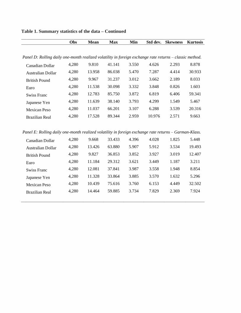
Table 1. Summary statistics of the data – Continued
Obs Mean Max Min Std dev. Skewness Kurtosis
Panel D: Rolling daily one-month realized volatility in foreign exchange rate returns – classic method.
Canadian Dollar 4,280 9.810 41.141 3.550 4.626 2.293 8.878
Australian Dollar 4,280 13.958 86.038 5.470 7.287 4.414 30.933
British Pound 4,280 9.967 31.237 3.012 3.662 2.189 8.033
Euro 4,280 11.538 30.098 3.332 3.848 0.826 1.603
Swiss Franc 4,280 12.783 85.750 3.872 6.819 6.406 59.341
Japanese Yen 4,280 11.639 38.140 3.793 4.299 1.549 5.467
Mexican Peso 4,280 11.037 66.201 3.107 6.288 3.539 20.316
Brazilian Real 4,280 17.528 89.344 2.959 10.976 2.571 9.663
Panel E: Rolling daily one-month realized volatility in foreign exchange rate returns – Garman-Klass.
Canadian Dollar 4,280 9.668 33.433 4.396 4.028 1.825 5.448
Australian Dollar 4,280 13.426 63.880 5.907 5.912 3.534 19.493
British Pound 4,280 9.827 36.853 3.852 3.927 3.019 12.407
Euro 4,280 11.184 29.312 3.621 3.449 1.187 3.211
Swiss Franc 4,280 12.081 37.841 3.987 3.558 1.948 8.854
Japanese Yen 4,280 11.328 33.864 3.885 3.570 1.632 5.296
Mexican Peso 4,280 10.439 75.616 3.760 6.153 4.449 32.502
Brazilian Real 4,280 14.464 59.885 3.734 7.829 2.369 7.924

Table 2. Accuracy of foreign exchange option-implied volatilities as forecasts of realized
volatilities.
This table contains the Mean Absolute Percentage Error (MAPE) obtained from using the
Bloomberg foreign exchange rate implied volatilities as the forecast of the subsequent realized
volatilities. Results are tabulated for one-month, three-month, and one-year option implied
foreign exchange volatilities as forecasts of realized volatilities calculated using both the
classical and the Glass-Karman methodologies.
Classical Method Garman-Klass Method 1-mo 3-mo 1-year 1-mo 3-mo 1-year
Mean Absolute Percentage Error (MAPE)
Canadian Dollar .283% .306% .326% .189% .231% .270%
Australian Dollar .683% .753% .810% .415% .472% .496%
British Pound .206% .202% .269% .167% .178% .231%
Euro .273% .265% .291% .180% .193% .235%
Swiss Franc .741% .697% .530% .285% .258% .258%
Japanese Yen .345% .322% .342% .233% .232% .275%
Mexican Peso .546% .561% .643% .441% .454% .486%
Brazilian Real 1.17% 1.32% 1.28% .609% .644% .639%
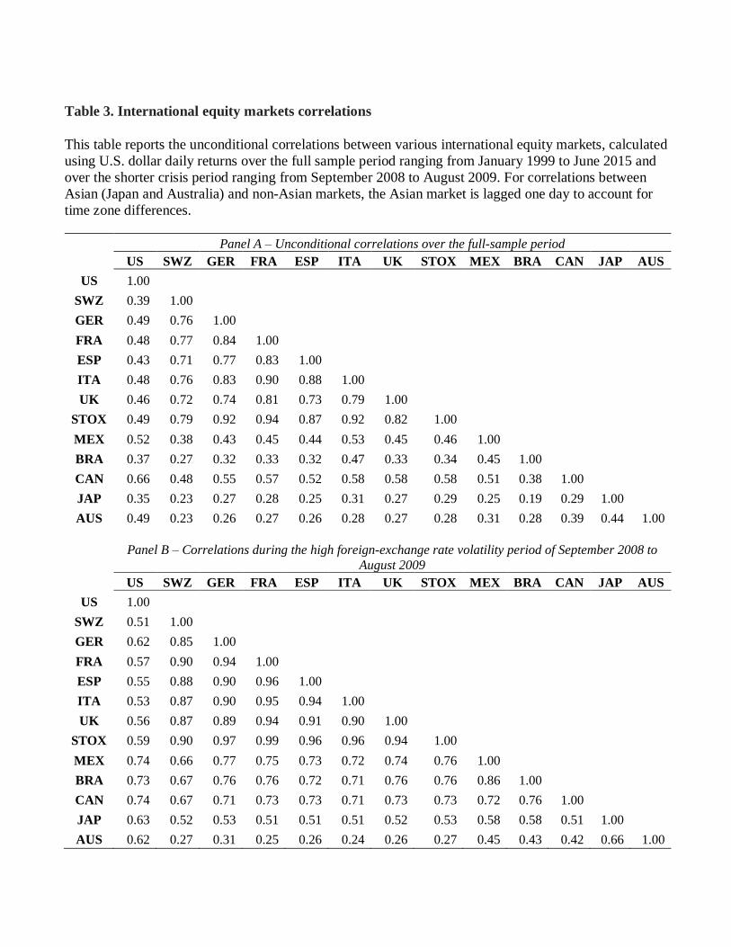
Table 3. International equity markets correlations
This table reports the unconditional correlations between various international equity markets, calculated
using U.S. dollar daily returns over the full sample period ranging from January 1999 to June 2015 and
over the shorter crisis period ranging from September 2008 to August 2009. For correlations between
Asian (Japan and Australia) and non-Asian markets, the Asian market is lagged one day to account for
time zone differences.
Panel A – Unconditional correlations over the full-sample period
US SWZ GER FRA ESP ITA UK STOX MEX BRA CAN JAP AUS
US 1.00
SWZ 0.39 1.00
GER 0.49 0.76 1.00
FRA 0.48 0.77 0.84 1.00
ESP 0.43 0.71 0.77 0.83 1.00
ITA 0.48 0.76 0.83 0.90 0.88 1.00
UK 0.46 0.72 0.74 0.81 0.73 0.79 1.00
STOX 0.49 0.79 0.92 0.94 0.87 0.92 0.82 1.00
MEX 0.52 0.38 0.43 0.45 0.44 0.53 0.45 0.46 1.00
BRA 0.37 0.27 0.32 0.33 0.32 0.47 0.33 0.34 0.45 1.00
CAN 0.66 0.48 0.55 0.57 0.52 0.58 0.58 0.58 0.51 0.38 1.00
JAP 0.35 0.23 0.27 0.28 0.25 0.31 0.27 0.29 0.25 0.19 0.29 1.00
AUS 0.49 0.23 0.26 0.27 0.26 0.28 0.27 0.28 0.31 0.28 0.39 0.44 1.00
Panel B – Correlations during the high foreign-exchange rate volatility period of September 2008 to
August 2009
US SWZ GER FRA ESP ITA UK STOX MEX BRA CAN JAP AUS
US 1.00
SWZ 0.51 1.00
GER 0.62 0.85 1.00
FRA 0.57 0.90 0.94 1.00
ESP 0.55 0.88 0.90 0.96 1.00
ITA 0.53 0.87 0.90 0.95 0.94 1.00
UK 0.56 0.87 0.89 0.94 0.91 0.90 1.00
STOX 0.59 0.90 0.97 0.99 0.96 0.96 0.94 1.00
MEX 0.74 0.66 0.77 0.75 0.73 0.72 0.74 0.76 1.00
BRA 0.73 0.67 0.76 0.76 0.72 0.71 0.76 0.76 0.86 1.00
CAN 0.74 0.67 0.71 0.73 0.73 0.71 0.73 0.73 0.72 0.76 1.00
JAP 0.63 0.52 0.53 0.51 0.51 0.51 0.52 0.53 0.58 0.58 0.51 1.00
AUS 0.62 0.27 0.31 0.25 0.26 0.24 0.26 0.27 0.45 0.43 0.42 0.66 1.00
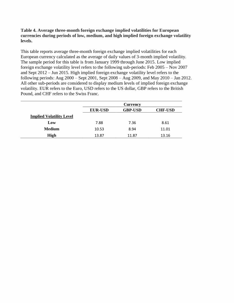
Table 4. Average three-month foreign exchange implied volatilities for European
currencies during periods of low, medium, and high implied foreign exchange volatility
levels.
This table reports average three-month foreign exchange implied volatilities for each
European currency calculated as the average of daily values of 3-month implied volatility.
The sample period for this table is from January 1999 through June 2015. Low implied
foreign exchange volatility level refers to the following sub-periods: Feb 2005 – Nov 2007
and Sept 2012 – Jun 2015. High implied foreign exchange volatility level refers to the
following periods: Aug 2000 – Sept 2001, Sept 2008 – Aug 2009, and May 2010 – Jan 2012.
All other sub-periods are considered to display medium levels of implied foreign exchange
volatility. EUR refers to the Euro, USD refers to the US dollar, GBP refers to the British
Pound, and CHF refers to the Swiss Franc.
Currency
EUR-USD GBP-USD CHF-USD
Implied Volatility Level
Low 7.88 7.36 8.61
Medium 10.53 8.94 11.01
High 13.87 11.87 13.16
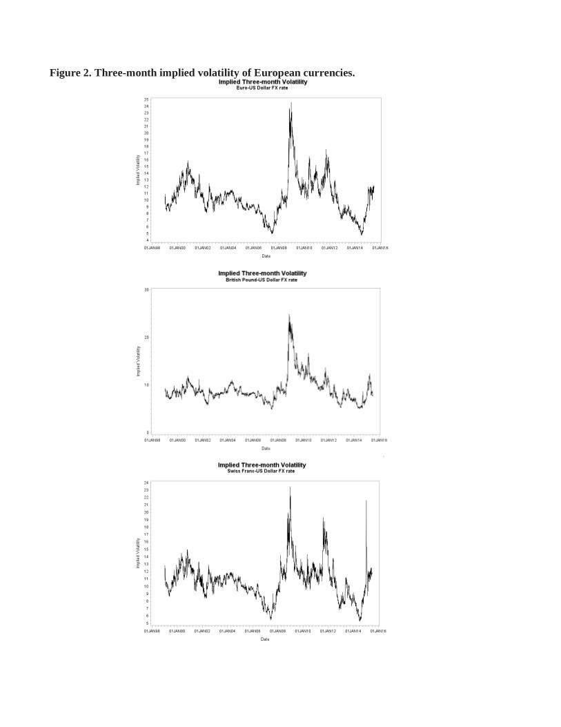
Figure 2. Three-month implied volatility of European currencies.
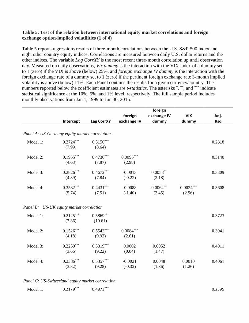
Table 5. Test of the relation between international equity market correlations and foreign
exchange option-implied volatilities (1 of 4)
Table 5 reports regressions results of three-month correlations between the U.S. S&P 500 index and
eight other country equity indices. Correlations are measured between daily U.S. dollar returns and the
other indices. The variable Lag CorrXY is the most recent three-month correlation up until observation
day. Measured on daily observations, Vix dummy is the interaction with the VIX index of a dummy set
to 1 (zero) if the VIX is above (below) 25%, and foreign exchange IV dummy is the interaction with the
foreign exchange rate of a dummy set to 1 (zero) if the pertinent foreign exchange rate 3-month implied
volatility is above (below) 11%. Each Panel contains the results for a given currency/country. The
numbers reported below the coefficient estimates are t-statistics. The asterisks *, **, and *** indicate
statistical significance at the 10%, 5%, and 1% level, respectively. The full sample period includes
monthly observations from Jan 1, 1999 to Jun 30, 2015.
Intercept Lag CorrXY foreign
exchange IV
foreign exchange IV
dummy VIX
dummy Adj. Rsq
Panel A: US-Germany equity market correlation
Model 1: 0.2724*** 0.5150*** 0.2818
(7.99) (8.64)
Model 2: 0.1955*** 0.4730*** 0.0095*** 0.3140
(4.63) (7.87) (2.98)
Model 3: 0.2826*** 0.4672*** -0.0013 0.0058** 0.3309
(4.89) (7.84) (-0.22) (2.18)
Model 4: 0.3532*** 0.4431*** -0.0088 0.0064** 0.0024*** 0.3608
(5.74) (7.51) (-1.40) (2.45) (2.96)
Panel B: US-UK equity market correlation
Model 1: 0.2125*** 0.5869*** 0.3723
(7.36) (10.61)
Model 2: 0.1526*** 0.5542*** 0.0084*** 0.3941
(4.18) (9.92) (2.61)
Model 3: 0.2259*** 0.5319*** 0.0002 0.0052 0.4011
(3.66) (9.22) (0.04) (1.47)
Model 4: 0.2386*** 0.5357*** -0.0021 0.0048 0.0010 0.4061
(3.82) (9.28) (-0.32) (1.36) (1.26)
Panel C: US-Switzerland equity market correlation
Model 1: 0.2179*** 0.4873*** 0.2395

(7.65) (7.73)
Model 2: 0.1567*** 0.4727*** 0.0063 0.2476
(3.05) (7.42) (1.43)
Model 3: 0.2187*** 0.4689*** -0.0012 0.0035 0.2531
(2.98) (7.36) (-0.16) (1.18)
Model 4: 0.2993*** 0.4332*** -0.0092 0.0037 0.0024*** 0.2793
(3.81) (6.75) (-1.12) (1.28) (2.61)
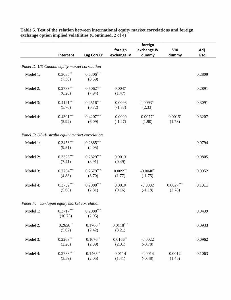
Table 5. Test of the relation between international equity market correlations and foreign
exchange option implied volatilities (Continued, 2 of 4)
Intercept Lag CorrXY foreign
exchange IV
foreign exchange IV
dummy VIX
dummy Adj. Rsq
Panel D: US-Canada equity market correlation
Model 1: 0.3035*** 0.5306*** 0.2809
(7.38) (8.59)
Model 2: 0.2783*** 0.5062*** 0.0047 0.2891
(6.26) (7.94) (1.47)
Model 3: 0.4121*** 0.4516*** -0.0093 0.0093** 0.3091
(5.70) (6.72) (-1.37) (2.33)
Model 4: 0.4301*** 0.4207*** -0.0099 0.0077* 0.0015* 0.3207
(5.92) (6.09) (-1.47) (1.90) (1.78)
Panel E: US-Australia equity market correlation
Model 1: 0.3453*** 0.2885*** 0.0794
(9.51) (4.05)
Model 2: 0.3325*** 0.2829*** 0.0013 0.0805
(7.41) (3.91) (0.49)
Model 3: 0.2734*** 0.2679*** 0.0099* -0.0048* 0.0952
(4.88) (3.70) (1.77) (-1.75)
Model 4: 0.3752*** 0.2088*** 0.0010 -0.0032 0.0027*** 0.1311
(5.68) (2.81) (0.16) (-1.18) (2.78)
Panel F: US-Japan equity market correlation
Model 1: 0.3717*** 0.2088*** 0.0439
(10.75) (2.95)
Model 2: 0.2656** 0.1700** 0.0118*** 0.0933
(5.62) (2.42) (3.21)
Model 3: 0.2263*** 0.1676** 0.0166** -0.0022 0.0962
(3.28) (2.39) (2.31) (-0.78)
Model 4: 0.2788*** 0.1465** 0.0114 -0.0014 0.0012 0.1063
(3.59) (2.05) (1.41) (-0.48) (1.45)
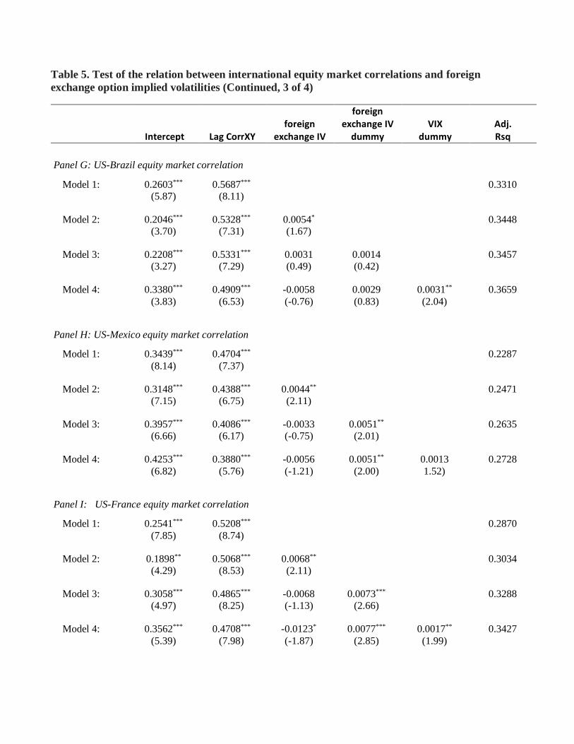
Table 5. Test of the relation between international equity market correlations and foreign
exchange option implied volatilities (Continued, 3 of 4)
Intercept Lag CorrXY foreign
exchange IV
foreign exchange IV
dummy VIX
dummy Adj. Rsq
Panel G: US-Brazil equity market correlation
Model 1: 0.2603*** 0.5687*** 0.3310
(5.87) (8.11)
Model 2: 0.2046*** 0.5328*** 0.0054* 0.3448
(3.70) (7.31) (1.67)
Model 3: 0.2208*** 0.5331*** 0.0031 0.0014 0.3457
(3.27) (7.29) (0.49) (0.42)
Model 4: 0.3380*** 0.4909*** -0.0058 0.0029 0.0031** 0.3659
(3.83) (6.53) (-0.76) (0.83) (2.04)
Panel H: US-Mexico equity market correlation
Model 1: 0.3439*** 0.4704*** 0.2287
(8.14) (7.37)
Model 2: 0.3148*** 0.4388*** 0.0044** 0.2471
(7.15) (6.75) (2.11)
Model 3: 0.3957*** 0.4086*** -0.0033 0.0051** 0.2635
(6.66) (6.17) (-0.75) (2.01)
Model 4: 0.4253*** 0.3880*** -0.0056 0.0051** 0.0013 0.2728
(6.82) (5.76) (-1.21) (2.00) 1.52)
Panel I: US-France equity market correlation
Model 1: 0.2541*** 0.5208*** 0.2870
(7.85) (8.74)
Model 2: 0.1898** 0.5068*** 0.0068** 0.3034
(4.29) (8.53) (2.11)
Model 3: 0.3058*** 0.4865*** -0.0068 0.0073*** 0.3288
(4.97) (8.25) (-1.13) (2.66)
Model 4: 0.3562*** 0.4708*** -0.0123* 0.0077*** 0.0017** 0.3427
(5.39) (7.98) (-1.87) (2.85) (1.99)
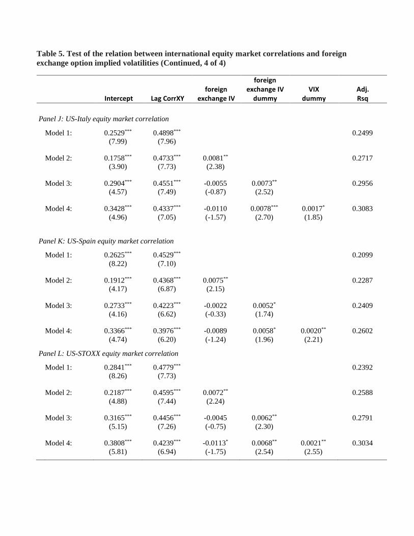
Table 5. Test of the relation between international equity market correlations and foreign
exchange option implied volatilities (Continued, 4 of 4)
Intercept Lag CorrXY foreign
exchange IV
foreign exchange IV
dummy VIX
dummy Adj. Rsq
Panel J: US-Italy equity market correlation
Model 1: 0.2529*** 0.4898*** 0.2499
(7.99) (7.96)
Model 2: 0.1758*** 0.4733*** 0.0081** 0.2717
(3.90) (7.73) (2.38)
Model 3: 0.2904*** 0.4551*** -0.0055 0.0073** 0.2956
(4.57) (7.49) (-0.87) (2.52)
Model 4: 0.3428*** 0.4337*** -0.0110 0.0078*** 0.0017* 0.3083
(4.96) (7.05) (-1.57) (2.70) (1.85)
Panel K: US-Spain equity market correlation
Model 1: 0.2625*** 0.4529*** 0.2099
(8.22) (7.10)
Model 2: 0.1912*** 0.4368*** 0.0075** 0.2287
(4.17) (6.87) (2.15)
Model 3: 0.2733*** 0.4223*** -0.0022 0.0052* 0.2409
(4.16) (6.62) (-0.33) (1.74)
Model 4: 0.3366*** 0.3976*** -0.0089 0.0058* 0.0020** 0.2602
(4.74) (6.20) (-1.24) (1.96) (2.21)
Panel L: US-STOXX equity market correlation
Model 1: 0.2841*** 0.4779*** 0.2392
(8.26) (7.73)
Model 2: 0.2187*** 0.4595*** 0.0072** 0.2588
(4.88) (7.44) (2.24)
Model 3: 0.3165*** 0.4456*** -0.0045 0.0062** 0.2791
(5.15) (7.26) (-0.75) (2.30)
Model 4: 0.3808*** 0.4239*** -0.0113* 0.0068** 0.0021** 0.3034
(5.81) (6.94) (-1.75) (2.54) (2.55)
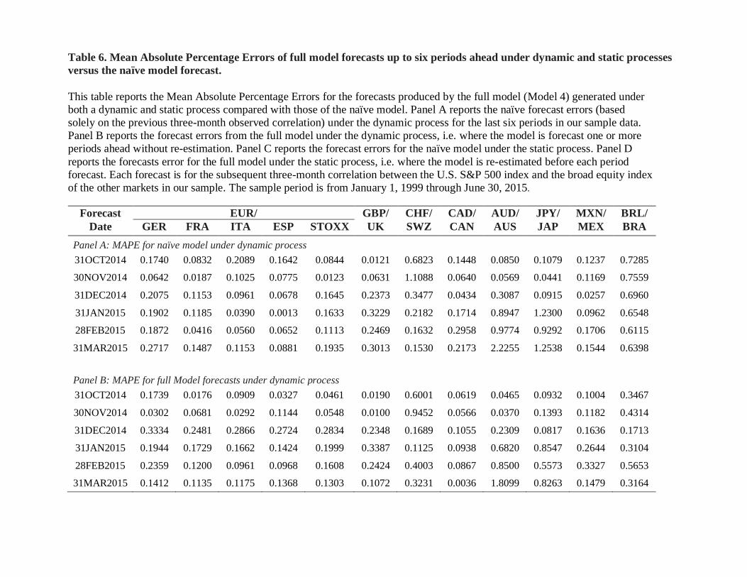
Table 6. Mean Absolute Percentage Errors of full model forecasts up to six periods ahead under dynamic and static processes
versus the naïve model forecast.
This table reports the Mean Absolute Percentage Errors for the forecasts produced by the full model (Model 4) generated under
both a dynamic and static process compared with those of the naïve model. Panel A reports the naïve forecast errors (based
solely on the previous three-month observed correlation) under the dynamic process for the last six periods in our sample data.
Panel B reports the forecast errors from the full model under the dynamic process, i.e. where the model is forecast one or more
periods ahead without re-estimation. Panel C reports the forecast errors for the naïve model under the static process. Panel D
reports the forecasts error for the full model under the static process, i.e. where the model is re-estimated before each period
forecast. Each forecast is for the subsequent three-month correlation between the U.S. S&P 500 index and the broad equity index
of the other markets in our sample. The sample period is from January 1, 1999 through June 30, 2015.
Forecast EUR/ GBP/ CHF/ CAD/ AUD/ JPY/ MXN/ BRL/
Date GER FRA ITA ESP STOXX UK SWZ CAN AUS JAP MEX BRA
Panel A: MAPE for naïve model under dynamic process
31OCT2014 0.1740 0.0832 0.2089 0.1642 0.0844 0.0121 0.6823 0.1448 0.0850 0.1079 0.1237 0.7285
30NOV2014 0.0642 0.0187 0.1025 0.0775 0.0123 0.0631 1.1088 0.0640 0.0569 0.0441 0.1169 0.7559
31DEC2014 0.2075 0.1153 0.0961 0.0678 0.1645 0.2373 0.3477 0.0434 0.3087 0.0915 0.0257 0.6960
31JAN2015 0.1902 0.1185 0.0390 0.0013 0.1633 0.3229 0.2182 0.1714 0.8947 1.2300 0.0962 0.6548
28FEB2015 0.1872 0.0416 0.0560 0.0652 0.1113 0.2469 0.1632 0.2958 0.9774 0.9292 0.1706 0.6115
31MAR2015 0.2717 0.1487 0.1153 0.0881 0.1935 0.3013 0.1530 0.2173 2.2255 1.2538 0.1544 0.6398
Panel B: MAPE for full Model forecasts under dynamic process
31OCT2014 0.1739 0.0176 0.0909 0.0327 0.0461 0.0190 0.6001 0.0619 0.0465 0.0932 0.1004 0.3467
30NOV2014 0.0302 0.0681 0.0292 0.1144 0.0548 0.0100 0.9452 0.0566 0.0370 0.1393 0.1182 0.4314
31DEC2014 0.3334 0.2481 0.2866 0.2724 0.2834 0.2348 0.1689 0.1055 0.2309 0.0817 0.1636 0.1713
31JAN2015 0.1944 0.1729 0.1662 0.1424 0.1999 0.3387 0.1125 0.0938 0.6820 0.8547 0.2644 0.3104
28FEB2015 0.2359 0.1200 0.0961 0.0968 0.1608 0.2424 0.4003 0.0867 0.8500 0.5573 0.3327 0.5653
31MAR2015 0.1412 0.1135 0.1175 0.1368 0.1303 0.1072 0.3231 0.0036 1.8099 0.8263 0.1479 0.3164
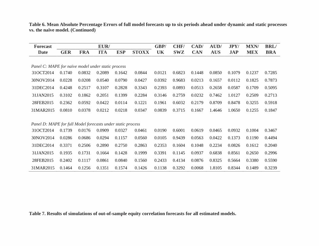
Table 6. Mean Absolute Percentage Errors of full model forecasts up to six periods ahead under dynamic and static processes
vs. the naïve model. (Continued)
Table 7. Results of simulations of out-of-sample equity correlation forecasts for all estimated models.
Forecast EUR/ GBP/ CHF/ CAD/ AUD/ JPY/ MXN/ BRL/
Date GER FRA ITA ESP STOXX UK SWZ CAN AUS JAP MEX BRA
Panel C: MAPE for naïve model under static process
31OCT2014 0.1740 0.0832 0.2089 0.1642 0.0844 0.0121 0.6823 0.1448 0.0850 0.1079 0.1237 0.7285
30NOV2014 0.0228 0.0208 0.0540 0.0790 0.0427 0.0392 0.9683 0.0213 0.1657 0.0112 0.1825 0.7873
31DEC2014 0.4248 0.2517 0.3107 0.2828 0.3343 0.2393 0.0893 0.0513 0.2658 0.0587 0.1709 0.5095
31JAN2015 0.3102 0.1862 0.2051 0.1399 0.2284 0.3146 0.2759 0.0232 0.7462 1.0127 0.2509 0.2713
28FEB2015 0.2362 0.0592 0.0422 0.0114 0.1221 0.1961 0.6032 0.2179 0.8709 0.8478 0.3255 0.5918
31MAR2015 0.0810 0.0378 0.0212 0.0218 0.0347 0.0839 0.3715 0.1667 1.4646 1.0650 0.1255 0.1847
Panel D: MAPE for full Model forecasts under static process
31OCT2014 0.1739 0.0176 0.0909 0.0327 0.0461 0.0190 0.6001 0.0619 0.0465 0.0932 0.1004 0.3467
30NOV2014 0.0286 0.0686 0.0294 0.1157 0.0560 0.0105 0.9439 0.0563 0.0422 0.1373 0.1190 0.4494
31DEC2014 0.3371 0.2506 0.2890 0.2750 0.2863 0.2353 0.1604 0.1048 0.2234 0.0826 0.1612 0.2040
31JAN2015 0.1935 0.1731 0.1664 0.1428 0.1999 0.3391 0.1145 0.0937 0.6838 0.8561 0.2650 0.2996
28FEB2015 0.2402 0.1117 0.0861 0.0840 0.1560 0.2433 0.4134 0.0876 0.8325 0.5664 0.3380 0.5590
31MAR2015 0.1464 0.1256 0.1351 0.1574 0.1426 0.1138 0.3292 0.0068 1.8105 0.8344 0.1489 0.3239

This table reports the Mean Absolute Percent Errors for the forecasts produced by all models tested, including the naïve forecast
model. The relation for models 1 through 4 are listed below the table. Forecasts are obtained by one-period ahead rolling regressions
starting with the first five years of data and then re-estimating them rolling forward one month at a time. The sample period is from
January 1, 1999 through June 30, 2015. The forecasts for correlations one-period ahead obtained are then compared to the actual
subsequent three-month correlations. The difference between the forecast and the actual subsequent value is used to calculate the
mean absolute percent error reported below. In the calculation of MAPE we exclude instances where the coefficient for the pertinent
independent variable in each model is not statistically significant at the 10% level or better. The number of forecasts included in the
calculation of each MAPE is shown above each percentage error.
EUR/ GBP/ CHF/ CAD/ AUD/ JPY/ MXN/ BRL/
Model GER FRA ITA ESP STOXX UK SWZ CAN AUS JAP MEX BRA
Naïve # forecasts 132 132 132 132 132 132 132 132 132 132 132 132
MAPE 0.2151 0.2123 0.2306 0.2240 0.2059 0.2172 0.5043 0.2084 0.4435 0.4435 0.1315 0.4514
1 # forecasts 120 76 95 66 94 88 112 118 70 27 79 88
MAPE 0.2223 0.1499 0.1797 0.1679 0.1552 0.1489 0.4243 0.2137 0.2121 0.1984 0.1268 0.5469
2 # forecasts 56 54 71 61 54 39 16 50 13 71 29 33
MAPE 0.1598 0.1372 0.1583 0.1562 0.1449 0.1444 0.4944 0.1408 0.1634 0.2685 0.1799 1.1302
3 # forecasts 69 80 76 85 72 28 3 56 0 4 26 11
MAPE 0.1652 0.1782 0.1962 0.1634 0.1741 0.1458 0.3696 0.3590 nm 0.2557 0.1169 0.8481
4 # forecasts 74 67 70 107 81 74 71 68 99 43 57 5
MAPE 0.2664 0.2619 0.2603 0.2065 0.2371 0.3235 0.5763 0.2731 0.6016 0.3078 0.1891 0.0366
Model 1: Corr_XY = Lag Corr_XY
Model 2: Corr_XY = Lag Corr_XY + foreign exchange_IV
Model 3: Corr_XY = Lag Corr_XY + foreign exchange_IV + foreign exchange dummy
Model 4: Corr_XY = Lag Corr_XY + foreign exchange_IV + foreign exchange dummy + VIX dummy

APPENDICES (A, B, C, AND D)
APPENDIX A
Attributed to economist John B. Taylor (1993), the Taylor rule dictates how central banks
should set the nominal interest rate in response to changes in inflation and GDP. Mathematically,
the rule is expressed as:
𝑟𝑡 = 𝜋𝑡 + 𝑟𝑡∗ + 𝜆𝜋(𝜋𝑡 − 𝜋𝑡
∗) + 𝜆𝑦(𝑦𝑡 − 𝑦𝑡∗) (A.1)
where 𝑟𝑡 represents the nominal short-term interest rate at time t, 𝜋𝑡 is the inflation at time t, 𝜋𝑡∗
is the target inflation rate, 𝑟𝑡∗ is the equilibrium real interest rate, 𝑦𝑡 is the log of real GDP and
𝑦𝑡∗ is the log of GDP potential. Additionally, the rule requires that both coefficients 𝜆𝜋 and 𝜆𝑦 be
positive. This means that according to the Taylor rule, interest rates should be set higher when
inflation is above target or when GDP is above its potential. As a rule of thumb, Taylor (1993)
suggests that 𝜆𝜋 = 𝜆𝑦 = 0.5. Under this assumption, when inflation rises by 1% equation (A.1)
would imply that the nominal interest rate should be raised by 1.5%. Conversely, should GDP
decline by 1%, the appropriate response would be to cut nominal rates by 0.5%. In more general
terms, equation (A.1) implies that the proper response for a 1% increase in inflation should be to
raise nominal interest rates by more than 1% since 𝜆𝜋 > 0 and the combined coefficient on 𝜋𝑡 is
(1 + 𝜆𝜋). Therefore, assuming financial markets use the Taylor rule to derive nominal interest
rate expectations for the U.S. we have:
𝔼𝑡𝑟𝑈𝑆,𝑡+1 = (1 + 𝜆𝜋)𝔼𝑡[𝜋𝑈𝑆,𝑡+1+𝑖] +𝜆𝑦𝔼𝑡[𝑦𝑈𝑆,𝑡+1] + 𝑟𝑈𝑆∗ (A.2)
where 𝑦𝑈𝑆,𝑡 represents the difference between the log of current and potential GDP. The
expression for interest rate expectation for Germany in the Euro zone can be expressed
analogously. For consistency with empirical evidence, foreign central banks are assumed to also
increase nominal rates when their currency depreciates relative to the US dollar. Clarida, Gali,

and Gertler (1998) demonstrate that to be the case for German and Japanese central banks. With
this additional term, the expression for expected nominal rates in Germany analogous to equation
(A.2) is:
𝔼𝑡𝑟𝐸𝑈𝑅,𝑡+1 = (1 + 𝜆𝜋)𝔼𝑡[π𝐸𝑈𝑅,𝑡+1+𝑖] +𝜆𝑦𝔼𝑡[𝑦𝐸𝑈𝑅,𝑡+1] + 𝑟𝐸𝑈𝑅∗ − 𝜆𝜀𝔼𝑡𝜉𝑡+1 (A.3)
where 𝜉𝑡 ≡ 𝑠𝑡 + 𝑝𝐸𝑈𝑅,𝑡 − 𝑝𝑈𝑆,𝑡 is the real exchange rate. Assuming that the equilibrium real
exchange rate in the U.S. and Germany are the same and subtracting equation (A.2) from (A.3)
yields:
𝔼𝑡[𝑟𝐸𝑈𝑅,𝑡+1 − 𝑟𝑈𝑆,𝑡+1] = (1 + 𝜆𝜋)𝔼𝑡[π𝐸𝑈𝑅,𝑡+1+𝑖 − π𝑈𝑆,𝑡+1+𝑖] +
𝜆𝑦𝔼𝑡[𝑦𝐸𝑈𝑅,𝑡+1 − 𝑦𝑈𝑆,𝑡+1] − 𝜆𝜉𝔼𝑡𝜉𝑡+1
(A.4)
which is the expression in equation (4).
APPENDIX B
Equation (3) reads: 𝔼𝑡𝑆𝑡+1 = 𝔼𝑡𝑆𝑡+2+𝔼𝑡[𝑟𝐸𝑈𝑅,𝑡+1 − 𝑟𝑈𝑆,𝑡+1] (B.1)
Substituting the expression for the expected nominal rate difference between Germany and the
U.S. in equation (A.4) into the second term of equation (B.1) yields:
𝔼𝑡𝑆𝑡+1 = 𝔼𝑡 𝑆𝑡+2+(1 + 𝜆𝜋)𝔼𝑡[π𝐸𝑈𝑅,𝑡+1+𝑖 − π𝑈𝑆,𝑡+1+𝑖] + 𝜆𝑦𝔼𝑡[𝑦𝐸𝑈𝑅,𝑡+1
− 𝑦𝑈𝑆,𝑡+1] − 𝜆𝜉𝔼𝑡𝜉𝑡+1
(B.2)
Plugging in the expression for real exchange rate 𝜉𝑡 ≡ 𝑠𝑡 + 𝑝𝐸𝑈𝑅,𝑡 − 𝑝𝑈𝑆,𝑡 into (B.2) we have:
𝔼𝑡𝑆𝑡+1 = 𝔼𝑡 𝑆𝑡+2+(1 + 𝜆𝜋)𝔼𝑡[π𝐸𝑈𝑅,𝑡+1+𝑖 − π𝑈𝑆,𝑡+1+𝑖] + 𝜆𝑦𝔼𝑡[𝑦𝐸𝑈𝑅,𝑡+1
− 𝑦𝑈𝑆,𝑡+1] − 𝜆𝜉𝔼𝑡[𝑆𝑡+1 + 𝑝𝐸𝑈𝑅,𝑡+1 − 𝑝𝑈𝑆,𝑡+1] (B.3)

Bringing the term with 𝜆𝜉𝔼𝑡𝑆𝑡+1 to the left hand side of equation (B.3) we then have:
(1 + 𝜆𝜉)𝔼𝑡𝑆𝑡+1 = 𝔼𝑡 𝑆𝑡+2+(1 + 𝜆𝜋)𝔼𝑡[π𝐸𝑈𝑅,𝑡+1+𝑖 − π𝑈𝑆,𝑡+1+𝑖]
+𝜆𝑦𝔼𝑡[𝑦𝐸𝑈𝑅,𝑡+1 − 𝑦𝑈𝑆,𝑡+1] − 𝜆𝜉𝔼𝑡[𝑝𝐸𝑈𝑅,𝑡+1 − 𝑝𝑈𝑆,𝑡+1]
(B.4)
Now let us define 𝛾 = 1 (1 + 𝜆𝜉)⁄ < 1, since 𝜆𝜉 > 0. Expressing 𝜆𝜉 in terms of 𝛾 and
substituting into equation (B.4) yields:
(1 𝛾⁄ )𝔼𝑡𝑆𝑡+1 = 𝔼𝑡 𝑆𝑡+2+(1 + 𝜆𝜋)𝔼𝑡[π𝐸𝑈𝑅,𝑡+1+𝑖 − π𝑈𝑆,𝑡+1+𝑖]
+𝜆𝑦𝔼𝑡[𝑦𝐸𝑈𝑅,𝑡+1 − 𝑦𝑈𝑆,𝑡+1] + (1 − 𝛾
𝛾)𝔼𝑡[𝑝𝑈𝑆,𝑡+1 − 𝑝𝐸𝑈𝑅,𝑡+1]
(B.5)
By defining:
𝑓𝑡 = (1 + 𝜆𝜋)[π𝐸𝑈𝑅,𝑡+1 − π𝑈𝑆,𝑡+1] +𝜆𝑦[𝑦𝐸𝑈𝑅,𝑡 − 𝑦𝑈𝑆,𝑡] + (
1 − 𝛾
𝛾) [𝑝𝑈𝑆,𝑡
− 𝑝𝐸𝑈𝑅,𝑡]
(B.5)
Equation (B.5) can be simplified as:
𝔼𝑡𝑆𝑡+1 = 𝛾𝔼𝑡𝑆𝑡+2+𝛾𝔼𝑡𝑓𝑡+1 (B.6)
Iterating equation (B.6) forward one period, it follows that:
𝔼𝑡𝑆𝑡+2 = 𝛾𝔼𝑡𝑆𝑡+3+𝛾𝔼𝑡𝑓𝑡+2 (B.7)
Substituting the result for 𝔼𝑡𝑆𝑡+2 from (B.7) into equation (B.6) yields:
𝔼𝑡𝑆𝑡+1 = 𝛾2𝔼𝑡 𝑆𝑡+3+𝛾2𝔼𝑡𝑓𝑡+2 + 𝛾𝔼𝑡𝑓𝑡+1 (B.8)
Iterating forward equation (B.7) and substituting the result for 𝔼𝑡𝑆𝑡+3 into equation (B.8) yields:
𝔼𝑡𝑆𝑡+1 = 𝛾3𝔼𝑡 𝑆𝑡+4+𝛾3𝔼𝑡𝑓𝑡+3 + 𝛾2𝔼𝑡𝑓𝑡+2 + 𝛾𝔼𝑡𝑓𝑡+1 (B.9)

Notice that if equation (B.6) is iterated indefinitely, the first term will become zero as
𝔼𝑡 limi→∞
𝛾𝑖 𝑠𝑡+𝑖 = 0 since 𝛾 = 1 (1 + 𝜆𝜉)⁄ < 1. The terms with 𝛾𝑖𝔼𝑡𝑓𝑡+𝑖 become an infinite sum.
Thus,
𝔼𝑡𝑆𝑡+1 = 𝔼𝑡∑𝛾𝑖
∞
𝑖=1
𝑓𝑡+1 (B.10)
which is the expression in equation (5).
APPENDIX C Equation (10) reads: 𝑟𝐸𝑈𝑅,𝑡 − r𝑈𝑆,𝑡 = 𝐾1,𝑡[𝑦𝐸𝑈𝑅,𝑡 − 𝑦𝑈𝑆,𝑡] + 𝐾2,𝑡 (C.1)
Recall from the definition of the Taylor Rule in appendix A equation (A.1), 𝑦𝑡 is the log of real
GDP. Thus, by defining 𝑌𝑡 to be real GDP, equation (C.1) can be rewritten as:
𝑟𝐸𝑈𝑅,𝑡 − r𝑈𝑆,𝑡 = 𝐾1,𝑡[log𝑌𝐸𝑈𝑅,𝑡 − log 𝑌𝑈𝑆,𝑡] + 𝐾2,𝑡 (C.2)
Rearranging equation (C.2) and applying the logarithm property log𝑎
𝑏= log 𝑎 − log 𝑏, yields:
log
𝑌𝐸𝑈𝑅,𝑡𝑌𝑈𝑆,𝑡
=𝑟𝐸𝑈𝑅,𝑡 − r𝑈𝑆,𝑡 −𝐾2,𝑡
𝐾1,𝑡 (C.3)
It then follows that:
𝑌𝐸𝑈𝑅,𝑡𝑌𝑈𝑆,𝑡
= exp(𝑟𝐸𝑈𝑅,𝑡 − r𝑈𝑆,𝑡 −𝐾2,𝑡
𝐾1,𝑡) (C.4)
Defining 𝐾0,𝑡 = 𝑒𝑥𝑝 (𝐾2,𝑡
𝐾1,𝑡), equation (C.4) can be rewritten as:
𝐾0,𝑡
𝑌𝐸𝑈𝑅,𝑡𝑌𝑈𝑆,𝑡
=𝑒𝑟𝐸𝑈𝑅,𝑡 𝐾1,𝑡⁄
𝑒𝑟𝑈𝑆,,𝑡 𝐾1,𝑡⁄ (C.5)
which is equivalent to equation (11)
𝐾0,𝑡
𝑌𝐸𝑈𝑅,𝑡
𝑒𝑟𝐸𝑈𝑅,𝑡 𝐾1,𝑡⁄ =𝑌𝑈𝑆,𝑡
𝑒𝑟𝑈𝑆,,𝑡 𝐾1,𝑡⁄ (C.6)
APPENDIX D Because of the time series nature of our data, the key assumption in ordinary least square
regressions of independence in residuals would be violated. We account for the autocorrelation
of the errors via an autoregressive model for the random error. Specifically, the autoregressive
error model employed is:
𝑦𝑡 = 𝑥𝑡′𝛽 + 𝜐𝑡 (D.1)
𝜐𝑡 = 𝜑1𝜐𝑡−1 − 𝜑2𝜐𝑡−2 −⋯−𝜑𝑚𝜐𝑡−𝑚 + 𝜖𝑡 (D.2)
𝜖𝑡~𝐼𝑁(0, 𝜎2) (D.3)
In this model 𝜖𝑡 is assumed to be normally and independently distributed with a mean 0 and
variance 𝜎2 as expressed in relation (D.3). Regression coefficients 𝛽 and error model parameters
𝜑𝑡are estimated simultaneously to correct for the autocorrelation in the time series data.