Determination of As-Discarded Methane Potential in ...
122
EPA 600/R-18/087 May 2018 | www.epa.gov/ord Determination of As-Discarded Methane Potential in Residential and Commercial Municipal Solid Waste Office of Research and Development
Transcript of Determination of As-Discarded Methane Potential in ...

EPA 600/R-18/087 May 2018 | www.epa.gov/ord
Determination of As-Discarded Methane Potential in Residential and Commercial Municipal Solid Waste
Offi ce of Research and Development

Determination of As-Discarded Methane
Potential in Residential and Commercial
Municipal Solid Waste
Report
By Timothy G. Townsend, Giles W. Chickering, and Max J. Krause
Jacobs Technology and
Department of Environmental
Engineering Sciences
University of Florida, Gainesville, Florida
Prepared for:
Susan A. Thorneloe
U.S. Environmental Protection Agency
Office of Research and Development
National Risk Management Research Laboratory
Air & Energy Management Division
Research Triangle Park, NC 27711
Prepared by:
Jacobs Technology Inc.
Research Triangle Park, NC 27709
Contract EP-C-15-008
Work Assignment No: 3-007
November 2018

i
Notice
The U.S. Environmental Protection Agency through its Office of Research and Development
funded and managed the study described here under Contract EP-D-11-006 to Eastern
Research Group, Inc. This report has been subjected to the Agency’s peer and administrative
review and has been approved for publication as an EPA document.

ii
Abstract
Methane generation potential, L0, is a primary parameter of the first-order decay (FOD)
model used to predict municipal solid waste (MSW) landfill gas (LFG) generation. Previously
reported L0 values in the literature span a wide range, including estimates substantially lower
than the current United States Environmental Protection Agency (U.S. EPA) AP-42 default value
of 100 m3 CH4/Mg MSW. Most previous estimates were developed from waste composition
studies and default component L0 values or best-fit analysis based on measured landfill gas
collection and default collection efficiencies. This work took a waste compositional approach,
paired with individually measured methane generation potentials for each sample collected. This
study also addressed the fines fraction of MSW, which is frequently omitted in other studies. The
objective of this research was to measure methane potential in MSW samples obtained directly
from waste collection vehicles at the point of disposal to provide an updated sense of how
current residential and commercial MSW compares to the AP-42 value used in estimating
methane emissions for use in Clean Air Act emissions inventories.
Four sites were selected in Florida, Georgia, and North Carolina for this study. Ten-to-
twelve collection vehicles were selected and sorted at each site and the biodegradable fractions
were transported to the University of Florida Solid and Hazardous Waste Management (SHWM)
research laboratories for further analysis. A unique L0 value was determined for each of the 39
representative loads of waste studied, based on the physical properties and methane yields
assessed in the SHWM lab. The values were normally distributed with means expected to fall in
a 95% confidence interval between 74-86 m3 CH4/Mg MSW as-discarded. The overall mean L0
in this study was 80 m3 CH4/Mg MSW and while there was not a statistically significant
difference between the two groups, commercial MSW yields (95% CI of 77-92 m3 CH4/Mg
MSW) showed a higher average L0 than residential MSW (95% CI of 67-85 m3 CH4/Mg MSW).
“Fines” fractions were found to contribute an average of 19% of the total methane yield for each
load of MSW studied. In one load the fines contributed over 50% of the total methane generated.
If fines were omitted from this study completely, the average L0 calculated would have been 65
m3 CH4/Mg MSW as opposed to 80. These yields were paired with a total carbon analysis to
reveal that MSW has an average carbon content of 34% (dry mass C/dry mass total) with a 54:46
ratio of biogenic to fossil carbon in dry samples. On average 43% of biogenic carbon evolved to
carbon in CH4 or CO2 among all biodegradable waste under anaerobic conditions. These findings
showed residential and commercial MSW produced an average L0 lower than existing default
value but higher than estimates in some recent studies. Several loads of waste in this study
produced methane in excess of the current AP-42 value which suggests that the current value
may under estimate methane emissions.

iii
Foreword
The United States Environmental Protection Agency (U.S. EPA) is charged by Congress
with protecting the nation's land, air, and water resources. Under a mandate of national
environmental laws, the Agency strives to formulate and implement actions leading to a
compatible balance between human activities and the ability of natural systems to support and
nurture life. To meet this mandate, EPA's research program is providing data and technical
support for solving environmental problems today and building a science knowledge base
necessary to manage our ecological resources wisely, understand how pollutants affect our
health, and prevent or reduce environmental risks in the future.
The National Risk Management Research Laboratory (NRMRL) within the Office of
Research and Development (ORD) is the Agency's center for investigation of technological and
management approaches for preventing and reducing risks from pollution that threaten human
health and the environment. The focus of the Laboratory's research program is on methods and
their cost-effectiveness for prevention and control of pollution to air, land, water, and subsurface
resources; protection of water quality in public water systems; remediation of contaminated sites,
sediments and ground water; prevention and control of indoor air pollution; and restoration of
ecosystems. NRMRL collaborates with both public and private sector partners to foster
technologies that reduce the cost of compliance and to anticipate emerging problems. NRMRL's
research provides solutions to environmental problems by: developing and promoting
technologies that protect and improve the environment; advancing scientific and engineering
information to support regulatory and policy decisions; and providing the technical support and
information transfer to ensure implementation of environmental regulations and strategies at the
national, state, and community levels.
This publication was produced in support of ORD’s Air, Climate, and Energy FY16-19
Strategic Research Action Plan. EPA, along with other federal partners, is working in
collaboration with the Global Alliance for Clean Cookstoves to conduct research and provide
tools to inform decisions about clean cookstoves and fuels in developing countries. EPA
previously completed a life cycle assessment (LCA) comparing the environmental footprint of
current and potential fuels and fuel mixes used for cooking within India and China (Cashman et
al. 2016). This study furthers the initial work by expanding the LCA methodology to include
new cooking mix and electrical grid scenarios, additional sensitivity analyses, uncertainty
analyses, and includes a normalized presentation of results. This phase of work also expands the
geographic scope of the study to include both Kenya and Ghana. Study results will allow
researchers and policy-makers to quantify sustainability-related metrics from a systems
perspective.
Cynthia Sonich-Mullin, Director
National Risk Management Research Laboratory
Office of Research and Development
U.S. Environmental Protection Agency

iv
Acknowledgments
This work was sponsored by the United States Environmental Protection Agency under
the direction of Susan Thorneloe. The contract was managed by Jacobs Technology, Inc.; the
University of Florida served as a sub-contractor to Jacobs Technology, Inc. The authors thank
each of the host facilities and the many on-site employees who assisted with coordinating the
waste composition studies. Many thanks to all waste sorters (paid and volunteer) who made the
waste composition studies possible. The authors would like to recognize all undergraduate
research assistants that worked tirelessly in the laboratory to process and analyze more than 400
samples and run over 1,400 methane potential assays.

v
Table of Contents
Abstract ........................................................................................................................................... ii
Foreword ........................................................................................................................................ iii
Acknowledgments.......................................................................................................................... iv
Table of Contents .............................................................................................................................v
List of Figures ............................................................................................................................... vii
List of Tables ............................................................................................................................... viii
Acronyms and Abbreviations ........................................................................................................ ix
Introduction ......................................................................................................................................1
Materials and Methods .....................................................................................................................3
1.1 Experimental Approach ...........................................................................................3
1.2 Site Descriptions ......................................................................................................3
1.2.1 Lee County, Florida .................................................................................................3
1.2.2 Alachua County, FL .................................................................................................4
1.2.3 Athens-Clarke County, Georgia...............................................................................5
1.2.4 Durham County, North Carolina..............................................................................5
1.3 Sample Collection and Categorization Procedures ..................................................6
1.3.1 Collection of Representative Samples .....................................................................6
1.3.2 Safety Protocols .......................................................................................................8
1.3.3 MSW Composition Studies......................................................................................9
1.4 Laboratory Procedures ...........................................................................................13
1.4.1 Laboratory Sample Processing ..............................................................................13
1.4.2 Biochemical Methane Potential Assay ..................................................................14
1.5 Methane Generation Potential................................................................................15
1.6 Total Carbon Analysis ...........................................................................................16
1.7 Biogenic and Fossil Carbon Analysis ....................................................................16
1.8 Degradable Carbon Fraction ..................................................................................17
Results and Discussion ..................................................................................................................17
1.9 Waste Composition Studies ...................................................................................17
1.10 Moisture Content and Volatile Solids Content of MSW Components ..................20
1.11 Volatile Solids Analysis of the Fines Fractions .....................................................21
1.12 Ultimate Methane Yields of MSW Components by BMP.....................................23
1.13 Methane Generation Potential, L0, by Representative Sample ..............................30
1.14 Carbon Content in MSW Fractions........................................................................33
1.15 Biogenic and Fossil Carbon ...................................................................................35
1.16 Degradable Carbon Fraction ..................................................................................37
Conclusions ....................................................................................................................................41
References ......................................................................................................................................45
Appendices .....................................................................................................................................49
Appendix A. Waste Composition Data Sheet Template ....................................................49

vi
Appendix B. Moisture Content and Volatile Solids Content Data ....................................50
Appendix C. Fines Composition Data ...............................................................................58
Appendix D. Distributions of Methane Yields by MSW Component ...............................60
Appendix E. Waste Composition and L0 of Representative Samples ...............................68
Appendix F. Carbon Content in 39 Waste Collection Vehicles ......................................107

vii
List of Figures
Figure 1-1. Lee County, Highlighted in Red, is Located in Southwest Florida ..............................4
Figure 1-2. Alachua County is Highlighted in Red .........................................................................4
Figure 1-3. Athens-Clarke County is Highlighted in Red ...............................................................5
Figure 1-4. Durham County, North Carolina is Highlighted in Red ...............................................6
Figure 1-5. Rear-Loading (a), Side-Loading (b), Front-Loading Vehicles (c), and Compacting
Bins (d).................................................................................................................................7
Figure 1-6. Plan View of a Typical Waste Composition Study Site Arrangement .........................7
Figure 1-7. The UF SHWM Sorting Table Constructed to Increase Sorting Efficiency Using
Screens Instead of a Solid Surface .......................................................................................8
Figure 1-8. Materials that Passed the 4 in2 Screen and were Retained on the 1 in2 Mesh .............10
Figure 1-9. Material that Passed the 1 in2 Screen; a Mix of Biodegradable and Non-
Biodegradable Items ..........................................................................................................11
Figure 1-10. Field Sampling Technique ........................................................................................12
Figure 1-11. Comparison of Average Waste Composition in All Studied MSW Streams ............18
Figure 1-12. Comparison of Average Waste Composition in Residential MSW Streams ............19
Figure 1-13. Comparison of Average Waste Composition in Commercial MSW Streams ..........20
Figure 1-14. Average Moisture Content of MSW Components Collected During WCS ..............21
Figure 1-15. Average VS/TS of MSW Components Collected During WCS ...............................21
Figure 1-16. Composition of all Fines <2” Fractions ....................................................................22
Figure 1-17. Composition of all Fines <1” Fractions ....................................................................23
Figure 1-18. Modified Box and Whisker Plots Represent Median Methane Yield From all
Residential and Commercial MSW, 1st and 3rd Quartiles, and the Minimum and
Maximum Values Measured ..............................................................................................24
Figure 1-19. Yield Frequencies for All Pasteboard Samples .........................................................26
Figure 1-20. Yield Frequencies of Food and Soiled Paper ............................................................26
Figure -1-21. Distribution of Load L0 Values Measured in this Study ..........................................31
Figure 1-22. Frequency and Range of all L0 Values Measured from Commercial Samples .........32
Figure 1-23. Frequency and Range of All L0 Values Measured from Residential Samples .........32
Figure 1-24. Total Carbon Content (Dry Mass Carbon/Dry Mass Material) by Fraction. Boxes
Show Median, 1st and 3rd Quartiles of the Data for Each Fraction (Whiskers Represent
Minimum and Maximum Values) ......................................................................................34
Figure 1-25 Average Biogenic/Fossil Carbon Split for All Loads ................................................35
Figure 1-26. Comparison of L0 and Biogenic Carbon Content for each Load, Dur-Com 3
Excluded ............................................................................................................................36
Figure 1-27. Carbon Studied in this Research ...............................................................................38
Figure 1-28. Percent of Total Carbon Evolved to Both CH4 and CO2 by Component. Boxes Show
Median, 1st and 3rd Quartiles of the Data for Each Fraction. Whiskers Represent
Minimum and Maximum Values. Values Represent % of Dry Mass of Total Biogenic
Carbon that Evolved to Carbon in CH4 or CO2 .................................................................39
Figure 1-29. Comparison of Past Studies of L0 .............................................................................42

viii
Figure 1-30. Frequency and Range of All L0 Values Calculated Using Average Yields for each
Individual Organic Fraction ...............................................................................................43
List of Tables
Table 1-1. General Description of the Components of Interest .....................................................13
Table 1-2. Gas standards used for GC-TCD Calibration and QC Checks .....................................15
Table 1-3. Locations and Details of WCS Sites ............................................................................18
Table 1-4. Summarized Composition of Fines Fractions by Mass ................................................22
Table 1-5. Range of Methane Yields by OFMSW Component (mL CH4/ g VS) .........................25
Table 1-6. Comparison of Methane Yields in Dry and As-Discarded Form .................................27
Table 1-7. Methane Generation Parameters of Wood Products and Yard Waste ..........................29
Table 1-8. Methane Generation Parameters of Textiles and Diapers ............................................30
Table 1-9. Summary of All L0 Values Calculated by Representative Sample ..............................31
Table 1-10: Significance of Fines on L0 ........................................................................................33
Table 1-11. Total Carbon Content by Fraction (Dry Mass Carbon/Dry Mass Sample) ................34
Table 1-12. Average Biogenic/Fossil Carbon Split for All Loads. Based on Dry Mass
Carbon/Dry Mass Waste Composition ..............................................................................36
Table 1-13. Biogenic Carbon Content in Dry, Ground, Sorted Biodegradable Fines Fractions ...37
Table 1-14. Average Degradable Carbon Fraction by Location. Values Represent % of Dry Mass
of Total Biogenic Carbon that Evolved to Carbon in CH4 or CO2 ....................................38
Table 1-15. Average Degradable Carbon Fraction by Fraction. Values Represent Average % of
Total Carbon (Mass) in Dry Samples that Evolved to Carbon in CH4 or CO2 ..................40
Table 1-16. Comparison of L0 Values Calculated Using Average Yields and Individualized
Yields for Each Individual Organic Fraction .....................................................................43

ix
Acronyms and Abbreviations
AD – anaerobic digester
ANSI – American National Standards Institute
AP-42 – Compilation of Air Pollutant Emission Factors, published by US EPA
ASTM – American Society for Testing Materials
BF – biodegradable fraction
BMP – biochemical methane potential
C&D/C&DD – construction and demolition debris
CAA – Clean Air Act
EPA – Environmental Protection Agency
FINE – fines fraction in MSW
FOD – first-order decay (model)
GCCS – gas collection and control system
GC-TCD – gas chromatograph with thermal conductivity detector
HHW – household hazardous waste
HRT – hydraulic retention time
IF – inert fraction
INT – intermediate fines fraction in MSW
k – waste decay constant, or, gas generation rate constant for MSW landfills
L0 – methane generation potential
LFG – landfill gas
MC– moisture content of sample in percent water by mass
MRF – materials recovery facility
MSW – municipal solid waste
NIOSH –National Institute for Occupational Safety and Health
NSPS – New Source Performance Standards, published by US EPA
OFMSW – organic fraction of municipal solid waste
OMB – organic matter (boxboard) in MSW
OMC – organic matter (cardboard) in MSW
OMF – organic matter (food) in MSW
OMP – organic matter (paper) in MSW
OMSP – organic matter (soiled paper) in MSW

x
OMT – organic matter (textiles) in MSW
OMY – organic matter (yard waste) in MSW
PPE – personal protective equipment
SHWM – solid and hazardous waste management
UF – University of Florida
US – United States of America
VS – volatile solids content of sample in percent VS by mass
VS/TS – volatile solids/total solids content
WCS – waste composition study
WTE – waste to energy (facility)
1
Introduction
Methane generation potential, L0, is a primary parameter of the first-order decay (FOD)
model used for the regulation and prediction of municipal solid waste (MSW) landfill gas (LFG)
generation. In the United States (U.S.), there are currently two default regulatory values
attributed to L0. The first is the Clean Air Act (CAA) default, L0 = 170 m3 CH4/Mg MSW. This
value was promulgated under the New Source Performance Standards (NSPS) of the CAA and is
used by MSW containment facilities (landfills) to determine if a site requires a gas collection and
control system (GCCS) (U.S. EPA 1998). The second default value is the AP-42 L0 = 100
m3/Mg MSW. This value was determined by the Environmental Protection Agency (EPA) for
use in air emission inventories (U.S. EPA 2008). EPA also suggests this value for sizing a GCCS
along with expected receiving tonnages for the site.
As specified in NSPS, landfills cannot identify their own L0 for regulatory purposes,
though researchers have previously investigated this aspect in laboratory and field-scale
experiments (Bentley, Smith, and Schrauf 2005; Tolaymat et al. 2010). One experimental
method for determining the methane potential of a material is the biochemical methane potential
(BMP) assay, first developed by (Owen et al. 1979). Typically, MSW samples have been
collected before disposal (Eleazer et al. 1997) or excavated from landfills and transported to a
laboratory for further physical and chemical analyses (Kim, Jang, and Townsend 2011). There is
some concern that the existing protocols used to calculate L0 in this manner may yield inaccurate
results because of a limited sample size or the potential for sample contamination with soil or
other materials found within landfills.
Several studies report L0 values based on an average of different methodologies. Krause
et al. (2016) reported L0 values to vary from 20-223 m3 CH4/Mg MSW. While some more recent
studies support methane potential values similar to 100 m3 CH4/Mg MSW (Amini, Reinhart, and
Niskanen 2013; Wang et al. 2013), others suggest L0 may be as low as 60 m3 CH4/Mg MSW
(Eleazer et al. 1997; Staley and Barlaz 2009; Tolaymat et al. 2010). As many of these previous
studies are based on partially-degraded landfilled waste or waste composition studies with non-
uniform sampling and reporting methods, they may not necessarily reflect residential and
commercial waste entering landfills today. As an example, MSW landfills often accept materials
inherently low in methane yield (e.g., building materials and debris, soil, and/or exhausted
sludge). Additionally, some fractions of residential and commercial MSW (such as the fines
content) may be poorly represented in methane potential when applying standard waste
composition data to undefined materials.
To better characterize today’s waste streams for methane generation potential, a
methodology to determine L0 from as-discarded waste was developed for this study. This
methodology included the use of waste composition studies (WCSs) to categorize and collect the
biodegradable fractions of MSW.1 These same fractions were then analyzed by BMP assay and
paired with results of the WCS to calculate L0 for the waste stream. Physical characteristics
including moisture, volatile solids, and total carbon content were also determined throughout the
1 This report may use the term “organic” interchangeably with biodegradable. The authors recognize that within the
solid waste industry this is common practice, though technically a misnomer as many types of non-biodegradable
plastics are chemically organic (petroleum-based).

2
course of analysis to better understand the materials being tested. By measuring methane
potential in MSW samples obtained directly from waste collection vehicles at the point of
disposal, this investigation provided a detailed assessment of how current residential and
commercial MSW at the study sites compares to the EPA default value used in developing
emission inventories for the Clean Air Act.

3
Materials and Methods
1.1 Experimental Approach
Accurately determining L0 required multiple waste samples to form a representative
stream of MSW at each facility. This was achieved by selecting collection vehicles as they
arrived at waste disposal facilities and mixing the entire vehicle load with heavy machinery
before collecting a representative sample. Sample loads were separated on-site into
approximately 50 types of biodegradable and inert fractions (see Appendix A. Waste
Composition Data Sheet Template for full list). After categorization and weighing, the inert
materials were discarded on site while the biodegradable fractions were transported to the
University of Florida Solid SHWM research labs in Gainesville, Florida.
Biodegradable waste components were analyzed for moisture content and volatile solids
content based on standard methods described in Section 1.4.1. The BMP assay, used extensively
in this study, subjects a known quantity of biodegradable material to ideal anaerobic conditions
that would predict the ultimate methane generation potential of a material. Samples were
incubated and periodically measured for biogas generation and composition. The amount of
methane yielded from the known mass of material was used to back-calculate an L0 for each
individual waste material (L0i). Methane yields of each fraction were summed to determine the
L0 of each representative sample. These values were compared to previously reported values in
the literature and to the current U.S. regulatory defaults.
1.2 Site Descriptions
Four waste disposal facilities hosted the collection and waste sorting portions of this
study. Waste composition studies were performed on site in Florida, Georgia, and North Carolina
through 2014 and 2015. These facilities were required to have a covered tipping floor or suitable
sorting area for sorting actives. Sites were selected in an effort to sample from the widest
geographic range for this investigation and detailed in Table 1-1.
1.2.1 Lee County, Florida
Lee County is located in southwest Florida and has 618,000 residents (Figure 1-1). The
county is listed as having an overall recycling rate of 46%, with 37% recycling rates for glass,
94% for aluminum cans, 66% for plastic bottles, and 92% for steel cans (Florida Department of
Environmental Protection 2014). MSW is collected and hauled to the Lee County Resource
Recovery Facility, which includes an 1,800 ton per day waste-to-energy facility, a materials
recovery facility, yard waste composting operation, and construction and demolition debris
(C&DD) recycling facility. Twelve representative samples of residential and commercial MSW
were sorted and the biodegradable fraction was collected from the Lee County Resource
Recovery Facility in January 2014.

4
Figure 1-1. Lee County, Highlighted in Red, is Located in Southwest Florida
1.2.2 Alachua County, FL
Alachua County is located in north central Florida and has approximately 250,000
residents (Figure 1-2). The county is listed as having an overall recycling rate of 31%, with 43%
recycling rates for glass, 40% for aluminum cans, 44% for plastic bottles, and 28% for steel cans
(FDEP 2014). The dual stream collection system and relatively efficient MRF in Gainesville pair
with the University of Florida to hold a relatively high recycling rate relative to other counties in
North Florida. Alachua County Solid Waste Management operates the Leveda Brown
Environmental Park in Gainesville, FL, which includes a transfer station, a materials recovery
facility, a yard waste mulching operation, and a household hazardous waste (HHW) collection
center. MSW is collected from the county and hauled to New River Regional Landfill in Raiford,
FL. Five samples were sorted and collected in May 2014. All samples that originated at the
University of Florida and were considered commercial MSW.
Figure 1-2. Alachua County is Highlighted in Red

5
1.2.3 Athens-Clarke County, Georgia
Athens-Clarke County has a population of 115,000 and is located in northeastern Georgia
(Figure 1-3). A 2014 report by the county Solid Waste Department’s Recycling Division states
that over 20,500 tons of material was recovered through dual stream and single stream recycling
in Athens that year. An additional 22,873 tons of biosolids, yard waste, scrap metals and
electronic/hazardous wastes were also diverted from landfills. With these weights all being
reported as recycled (“diverted” technically a more appropriate label) by the county, the
calculated diversion rate was 44% relative to the 55,250 tons of waste disposed (Athens-Clarke
County 2014). The Athens-Clarke County Landfill is a lined, Subtitle D landfill comprised of
approximately 400 acres, accepts approximately 300 tpd of MSW and has an active gas
collection system and flare. A yard waste/biosolids composting system is also operated on site
and C&D wastes are diverted to the Oglethorpe County C&D landfill. The county-operated site
receives MSW from both public and private collection vehicles as well as residential drop-off. A
WCS was performed on site March 4 – 6, 2015.
Figure 1-3. Athens-Clarke County is Highlighted in Red
1.2.4 Durham County, North Carolina
Durham County has approximately 223,000 residents (Figure 1-4). The City of Durham
Solid Waste Management Department operates a transfer station at the Solid Waste Disposal
Facility. The waste generation rate is reported to be similar to the state average of approximately
0.98 tons of waste per person annually (State of North Carolina 2012). The overall recycling rate,
including composted organics, is 16% of the total measured MSW stream. The site also includes
a yard waste management facility, wastewater treatment plant, and a closed MSW landfill. The
transfer station accepts MSW from Durham County and some surrounding counties (e.g., Orange
County). Waste is hauled to the Brunswick Waste Management Facility in Lawrenceville,
Virginia. As of 2008, Durham recycled approximately 22% of its residential waste (Durham
County 2009). A WCS was performed on site March 23 – 26, 2015.

6
Figure 1-4. Durham County, North Carolina is Highlighted in Red
1.3 Sample Collection and Categorization Procedures
An abridged 3-4 day execution of the ASTM D5231-92 protocol was used during the
waste composition studies (ASTM International 2016). The word “sample” appears many times
in the following sections with several contextual meanings. A “representative sample” is the
quartered, mixed-MSW selected from the waste collection vehicle for sorting (ASTM
International 2016). A “component sample” or “laboratory sample” is one of the many different
biodegradable waste components that were collected after sorting and retained for physical and
methane potential analyses in the laboratory.
Sorting was performed in enclosed areas to prevent errors in data collection such as the
potential for increases in weight and moisture content from precipitation or winds that may cause
lightweight objects to leave the sorting area. Sorters wore personal protective equipment (PPE) at
all times during the WCS.
1.3.1 Collection of Representative Samples
WCS were performed to collect MSW component samples on an as-discarded basis (wet
weight). Waste collection vehicles were selected based on the source being residential or
commercial. Residential waste streams originate from single-family households and are typically
collected in rear-loading or side-loading waste collection vehicles. Commercial waste streams
may include multifamily residences and places of business. Only vehicles utilizing a compacting
mechanism (either on the truck or within the hauled container) were selected to avoid bulky
wastes that are large, heavy, and difficult to characterize as a single material type (e.g.,
mattresses made of metal, plastic, and textile). Figure 1-5 displays an example of each of these
vehicles that were selected in this study.
Selected trucks unloaded compacted MSW onto a tipping floor upon arrival. The hauling
company (or organization), vehicle number, source (residential or commercial), total waste
weight, and approximate route location were recorded on the data collection sheet (see Appendix
A. Waste Composition Data Sheet Template). To obtain a sufficient amount of organic fraction
samples (OFMSW), 10 – 12 vehicles were selected per facility. In the context of this report,
“organic” is meant to describe a biodegradable material found in MSW that is expected to
decompose under aerobic or anaerobic conditions.

7
Figure 1-5. Rear-Loading (a), Side-Loading (b), Front-Loading Vehicles (c), and Compacting Bins (d)
From the collection vehicle, MSW was mixed and quartered using equipment available
on site. Equipment included large front-end loaders or smaller skid-steers with bucket
attachments. Representative samples, approximately 90 to 136 kg each, were obtained from each
truck sorted (ASTM International 2016). The entire sample was transported to the sorting area
(Figure 1-6) adjacent to a sorting table (Figure 1-7).
Figure 1-6. Plan View of a Typical Waste Composition Study Site Arrangement

8
Figure 1-7. The UF SHWM Sorting Table Constructed to Increase Sorting Efficiency Using Screens Instead of a Solid Surface
The representative sample was then sorted categorized by material type, referred to as
“fractions” in this report. The weights of each fraction were recorded once the 90-136 kg sample
had been completely categorized to develop a waste composition specific to each representative
sample (each vehicle). Small 1-2 kg samples of each organic fraction of MSW (OFMSW) that
would contribute to methane generation in a landfill were recovered from each sorting event and
were transported in plastic bags to the SHWM labs for further analysis.
1.3.2 Safety Protocols
Personal protective equipment (PPE) was worn by researchers at all times. Nitrile gloves
were worn under a thicker rubber/cotton glove to give workers protection from sharp objects and
liquids. Additionally, workers were required to wear American National Standards Institute
(ANSI) Z87 approved safety glasses to protect the eyes and face. National Institute for
Occupational Safety and Health (NIOSH)-approved N95 respirators were made available to
protect workers from particulate matter. Boots and full-length pants were required. Full-body
Tyvek suits were also available for those that preferred greater protection.
Before sorting, representative samples were visually inspected for the presence of any
hazardous or medical wastes. Biomedical wastes (red bags or wastes improperly disposed in the
MSW stream) were reported to the host facility and discarded as per state regulations. Items to
scan for and remove without weighing were:
• Sharps
▪ Needles
▪ Razors
• Hazardous Waste

9
▪ Flammable
▪ Corrosive
▪ Reactive
▪ Toxic
• Infectious Waste
▪ Biomedical Bags (usually red bags)
▪ Syringes
▪ Items that may transfer diseases or infections to another person (bloody items)
Potentially biohazardous materials were detected in samples at Lee County and Durham
County. While the biohazardous material may have been disposed of within the technical
allowances of the law, sorting the material by hand posed too high of a risk. In Lee County, bags
were isolated and set aside for proper disposal. In Durham County, the entire representative
sample was deemed contaminated and that sample was abandoned for a substitute load. The
hauling company was notified and asked to properly dispose of the material at another site.
1.3.3 MSW Composition Studies
After the sample was deemed to be free of hazards, the waste was placed on the table top;
a 2 x 2” wire mesh screen that supported most items. Bags were opened and materials sorted into
the following categories:
• Paper
• Cardboard
• Plastic
• Textile
• Glass
• Metal
• Organics
• Construction and Demolition (C&D) debris
• Durable goods (including electronic wastes)
• Household hazardous waste (HHW; e.g., batteries, mercury-containing products)
Categories were further divided into approximately 50 total specific subcategories as
shown in the Waste Composition Data Form (see Appendix A. Waste Composition Data Sheet
Template). Containers for each subcategory were placed around the sorting table for easy access
to workers. The weight of each container was recorded before and after filling with each fraction
of the waste using a digital scale with maximum measurable weight 74 kg with +/- 0.05 kg
resolution (Measuretek).
The sorting table was equipped with two screens of different mesh sizes, shown in
Figure 1-8. Hand sorting occurred only on the top screen. This unique design allowed for faster,
more efficient sorting by removing lightweight and hard to identify materials from the sorting
area (by falling through to the second screen). The screen alleviated sorters from making difficult
categorical decisions for smaller objects, especially materials that were severely contaminated.

10
Many past studies have not implemented this screen system and require significantly more
sorting time for small components or left this fraction of waste unstudied.
Figure 1-8. Materials that Passed the 4 in2 Screen and were Retained on the 1 in2 Mesh
The waste captured by the bottom screen (referred to as Fines < 2”) and the waste that
falls to the tarp below (Fines <1”) were weighed and collected for further laboratory analysis.
Examples of the Fines are shown in Figure 1-9 and Figure 1-10.

11
Figure 1-9. Material that Passed the 1 in2 Screen;
a Mix of Biodegradable and Non-Biodegradable Items
The organic components of interest (OFMSW) were transported to the SHWM labs. The
subcategories expected to yield methane are specified in Table 1-1. The inert inorganic
substances, which were not expected to yield biogas, were weighed and discarded at the facility.
Figure 1-10 illustrates this process.

12
Figure 1-10. Field Sampling Technique
13
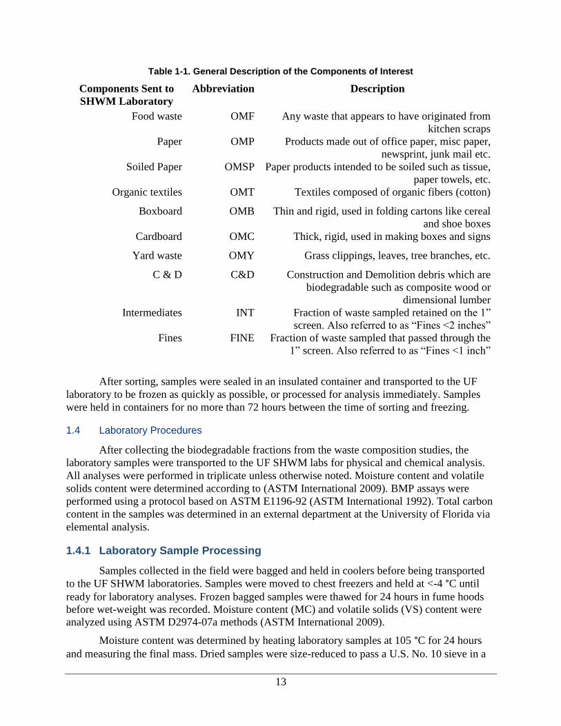
Table 1-1. General Description of the Components of Interest
Components Sent to
SHWM Laboratory
Abbreviation Description
Food waste OMF Any waste that appears to have originated from
kitchen scraps
Paper OMP Products made out of office paper, misc paper,
newsprint, junk mail etc.
Soiled Paper OMSP Paper products intended to be soiled such as tissue,
paper towels, etc.
Organic textiles OMT Textiles composed of organic fibers (cotton)
Boxboard OMB Thin and rigid, used in folding cartons like cereal
and shoe boxes
Cardboard OMC Thick, rigid, used in making boxes and signs
Yard waste OMY Grass clippings, leaves, tree branches, etc.
C & D
C&D Construction and Demolition debris which are
biodegradable such as composite wood or
dimensional lumber
Intermediates INT Fraction of waste sampled retained on the 1”
screen. Also referred to as “Fines <2 inches”
Fines FINE Fraction of waste sampled that passed through the
1” screen. Also referred to as “Fines <1 inch”
After sorting, samples were sealed in an insulated container and transported to the UF
laboratory to be frozen as quickly as possible, or processed for analysis immediately. Samples
were held in containers for no more than 72 hours between the time of sorting and freezing.
1.4 Laboratory Procedures
After collecting the biodegradable fractions from the waste composition studies, the
laboratory samples were transported to the UF SHWM labs for physical and chemical analysis.
All analyses were performed in triplicate unless otherwise noted. Moisture content and volatile
solids content were determined according to (ASTM International 2009). BMP assays were
performed using a protocol based on ASTM E1196-92 (ASTM International 1992). Total carbon
content in the samples was determined in an external department at the University of Florida via
elemental analysis.
1.4.1 Laboratory Sample Processing
Samples collected in the field were bagged and held in coolers before being transported
to the UF SHWM laboratories. Samples were moved to chest freezers and held at <-4 °C until
ready for laboratory analyses. Frozen bagged samples were thawed for 24 hours in fume hoods
before wet-weight was recorded. Moisture content (MC) and volatile solids (VS) content were
analyzed using ASTM D2974-07a methods (ASTM International 2009).
Moisture content was determined by heating laboratory samples at 105 °C for 24 hours
and measuring the final mass. Dried samples were size-reduced to pass a U.S. No. 10 sieve in a

14
mill (Fritsch Pulverisette 25, Germany) or industrial blender (Blendtec Designer 675, USA). The
dried ground material was collected in glass jars and stored at room temperature (approximately
20 °C). VS content was subsequently determined by heating the dried sample to 550 °C for four
hours. The difference between the post-ignition sample and the dry sample, divided by the dry
weight (the total solids), is calculated to be the VS content as a fraction of total solids (VS/TS).
VS content was used to determine the amount of material required for the BMP assay.
Prior to other physical analysis, the intermediate and the fine component samples were further
separated into biodegradable fines fractions and inert fines fractions (BFF and IFF, respectively)
by manual hand sorting and identification of non-methane-generating materials (e.g., glass,
plastics, metals, soil, etc.). The IFF, which consisted only of items that were clearly non-
biodegradable, was weighed and discarded. The BFF, which contained organic materials and
anything that was presumed biodegradable (e.g., used coffee grounds and filters, soil, sawdust,
etc.) was weighed and evaluated for MC and VS content as previously identified. The yields of
the individual fractions presented in the Results and Discussion section are representative of the
BFF itself, though the yields of the dry combined fractions are presented in

15
Appendix C. Fines Composition Data. The overall L0 values of each load factor in the IFF and
MC to provide an appropriate overall methane yield.
1.4.2 Biochemical Methane Potential Assay
The biochemical methane potential (BMP) assay used in this study was developed by and
adopted as a standard method (ASTM E1196-92, later withdrawn but still widely used) to
measure the quantity and composition of biogas. Many research groups still base their studies on
this method, though some have opted for larger reactors to incorporate a larger sample (Eleazer
et al. 1997; Wang and Barlaz 2016). This research follows Owen’s original method, requiring 0.2
g of ground and homogenized VS added to each 250-mL serum bottle. A nutrient broth,
anaerobic inoculum, and an oxygen indicator were added to the bottle while flushed with ultra-
pure nitrogen gas (Airgas, Gainesville FL) (Owen et al. 1979). Bottles were flushed for
approximately three minutes and sealed with a rubber septum and aluminum crimp closure.
Samples were incubated in an incubator (Fisher Scientific Isotemp, USA) at 35 °C.
Biogas samples were measured on the 7th, 14th, 21st, 28th, 42nd, and 56th day after
incubation using a gas-tight graduated syringe. Gas volume was measured by displacement of the
syringe barrel. The samples were analyzed in a gas chromatograph equipped with a thermal
conductivity detector (GC8A-TCD by Shimadzu, Japan). Column temperature was 100 °C and
oven temperature was 110 °C. The column used was a ShinCarbon ST Packed 2 m General
Column (Restek, USA). The carrier gas was ultra-high purity helium (Airgas, Gainesville FL).
Gas standards were used as calibration standards as well as quality control standards. A
50% or 15% methane standard, identified in Table 1-2, was analyzed every 9-12 samples as a
QC check. If the percent deviation was greater than 20%, the GC-TCD was recalibrated.

16
Table 1-2. Gas standards used for GC-TCD Calibration and QC Checks
Standard % CH4 % CO2 % O2 % N2 Source
High Methane 50 35 0 Balance Landtec North America, USA
Low Methane 15 15 0 Balance Landtec North America, USA
Oxygen 0 0 4 Balance Landtec North America, USA
A 12-liter anaerobic digester (AD) is maintained in the SHWM laboratory for several
years. The AD is the source of anaerobic inoculum for each BMP assay. The fed-batch digester
is housed in an incubator (Fisher Scientific Isotemp, USA). The digester is fed 1 g feed stock for
each 500 mL of reactor volume per day to achieve a hydraulic residence time (HRT) of 30 days.
The feedstock is ground dog food from the local supermarket, used in anaerobic digestion
experiments by other researchers because it is a cost-effective, degradable feedstock composed
of protein, carbohydrate, and sugars suitable for anaerobic microorganisms (Duran and Speece
1999; Lee et al. 2009). The pH of the digestate was measured and recorded in the AD logbook
regularly.
1.5 Methane Generation Potential
Methane generation potential (L0) describes the maximum amount of methane that can be
produced in a landfill from mixed MSW. Generation depends on the type of waste deposited and
can range from 6 and 270 m3 CH4/Mg MSW (U.S. EPA 2004). To determine this value
accurately, the ultimate methane yields measured in the BMP assays were applied to the physical
parameters (MC and VS) of the waste material to determine a material-specific methane
potential, L0i, as shown in equation 1.
𝐿0𝑖 =𝑚𝐿 𝐶𝐻4
𝑔 𝑉𝑆𝑖×
𝑔 𝑉𝑆𝑖
𝑔 𝑇𝑆𝑖× (1 −
𝑀𝐶𝑖
100) =
𝑚𝐿 𝐶𝐻4
𝑔𝑖=
𝑚3 𝐶𝐻4
𝑀𝑔 𝑀𝑆𝑊𝑖 (Equation 1)
With this information, the amount of potential methane generation of a specific waste
stream can be predicted. The individual L0 values were summed to determine the total methane
generation potential of the representative sample. The one sample Kolmogorov-Smirnov test for
normality using α = 0.05 was used to assess the normality for collections of yields calculated for
each fraction and the overall L0 values determined for residential, commercial, and combined
data sets.
𝐿0 = ∑ 𝐿0𝑖𝑛𝑖 (Equation 2)
The CH4 produced (mL per g of VS) was compared with the fraction of VS/total solids in
each sample, along with each respective MC to determine the mL of CH4 yielded from each g of
sample as-discarded. This value is equal to the m3 CH4/Mg MSW. The methane yield measured
in each bottle was converted to STP (0 °C and 1 atm) for comparison to other studies. Equation 3
shows how each bottle was converted to STP after being measured at 35 °C. All bottles were

17
assumed to remain at 35 °C during measurement, and the gas was assumed to be fully saturated
with water vapor, which has a partial pressure of 42 mm Hg. The partial pressure was subtracted
from the atmospheric pressure in the room at the time of measurement to obtain the volume of
dry gas measured. Finally, the volume of dry CH4 contributed by the inoculum was removed by
subtracting the average yield of the triplicate blanks created for each bottling session, leaving
only the methane contribution from the substrate itself.
𝑁𝑜𝑟𝑚𝑎𝑙𝑖𝑧𝑒𝑑 𝑦𝑖𝑒𝑙𝑑 𝑜𝑓 𝑑𝑟𝑦 𝐶𝐻4 @ 𝑆𝑇𝑃 (0 °𝐶 𝑎𝑛𝑑 1 𝑎𝑡𝑚) =
𝑚𝑙 𝐶𝐻4@ 35°𝐶
𝑔 𝑉𝑆 ∗ (
273𝐾
35𝐾 + 273𝐾) ∗ (
𝑃𝑟𝑒𝑠𝑠𝑢𝑟𝑒 𝑖𝑛 𝑟𝑜𝑜𝑚 − 42 𝑚𝑚 𝐻𝑔
760 𝑚𝑚 𝐻𝑔) − 𝐶𝐻4 𝑦𝑖𝑒𝑙𝑑 𝑓𝑟𝑜𝑚 𝑏𝑙𝑎𝑛𝑘𝑠 @ 𝑆𝑇𝑃
(Equation 3)
Once the yield of each sample was determined, the L0 of each truck sorted was
calculated. The individual L0 values for each component were weight-averaged based on waste
composition to determine the total methane generation potential of each load of waste sorted on a
tipping floor. Kolmogorov-Smirnov tests for normality using α = 0.05 were used to assess the
normality for the series of yields calculated for each fraction (e.g., all cardboard samples, all
newspaper, etc.) and the overall L0 values determined for residential, commercial, and combined
data sets. A 95% confidence interval was calculated for the full population of 39 L0 values by
applying a bootstrap sampling method with replacement, drawing from the total population of L0
values. Additional confidence intervals were calculated for the groups of residential and
commercial loads. After calculating L0 for each load of MSW sorted, 95% confidence intervals
were determined for all loads together as one set (n = 39) as well as confidence intervals for the
separated residential (n = 19) and commercial loads (n = 20). Standard deviations were
calculated for each set of values and before calculating confidence intervals with alpha of 0.05.
1.6 Total Carbon Analysis
The total carbon content of the dried, ground samples was determined through elemental
CNS macro analysis via a vario MACRO cube (Elementar) in the Extension Soil Testing Lab at
the University of Florida Institute of Food and Agricultural Sciences (IFAS). Samples between
1-2 g were assessed for total carbon content. IFAS ran standard samples through the instrument
every 10-15 samples as an internal QC throughout the analysis of all samples. The total carbon
analysis results were used to determine an average total carbon content of each combined waste
sample; this process is described in the Section 2.7.
1.7 Biogenic and Fossil Carbon Analysis
The total carbon content determined by IFAS was applied to the waste composition data
from each load to determine the total amount of carbon available from biogenic sources. None of
the non-biodegradable materials sorted were analyzed as these fractions were discarded after
each waste composition study. To determine a total carbon content of each waste load sorted, the
waste composition data was paired with the carbon content of each biodegradable fraction.
18
Carbon contents were assumed for non-biodegradable fractions. Plastics were assumed to consist
of 75% fossil carbon with the exception of composite plastics that were approximated to be
composed of 50% fossil carbons to account for non-plastic components. These values were based
on the presence and general chemical composition of the most prevalent forms of plastic (PET
with 63% carbon, HPDE with 86%, Polystyrene with 97%) and the assumption that all carbon in
plastics is fossil carbon. All non-plastic and non-biodegradable materials were assumed to
contain no fossil carbon or biogenic carbon. A weighted average carbon content for each truck
sorted was determined by multiplying the mass fraction of each category by the measured or
assumed carbon content of the respective category to account for the effect of waste
composition.
The heterogeneity of the fines fractions called for additional analysis beyond total carbon
content. These samples contained materials so small that even after sorting by hand as described
in Section 1.4.1 the material still had an undetermined amount of biogenic and fossil carbon. Six
total samples of sorted, dried, ground fines samples were analyzed by Beta Analytic (Miami, FL)
for biogenic/fossil carbon content via ASTM D6866 protocol. Samples between 20-25 g were
analyzed and selected based on relative methane yield. Three samples of fines <1” and three
fines <2” were analyzed, with a high, mid, and low methane yielding sample from each of the
two fractions selected. The samples chosen because they produced yields closest to the median,
25% and 75% quartile in the methane yield data set of fines.
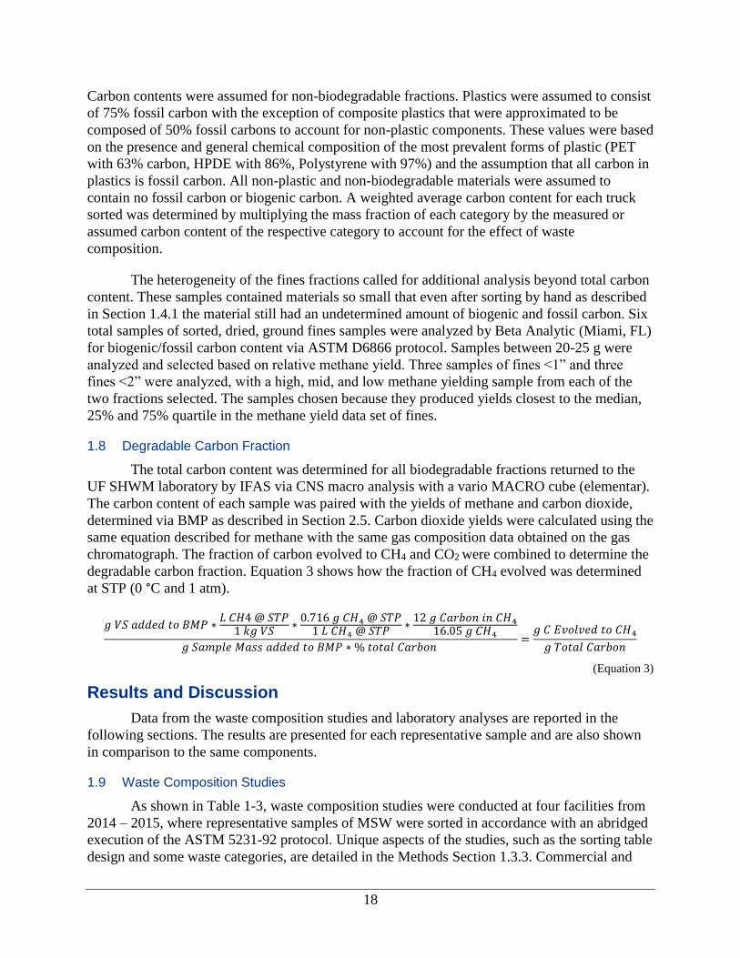
1.8 Degradable Carbon Fraction
The total carbon content was determined for all biodegradable fractions returned to the
UF SHWM laboratory by IFAS via CNS macro analysis with a vario MACRO cube (elementar).
The carbon content of each sample was paired with the yields of methane and carbon dioxide,
determined via BMP as described in Section 2.5. Carbon dioxide yields were calculated using the
same equation described for methane with the same gas composition data obtained on the gas
chromatograph. The fraction of carbon evolved to CH4 and CO2 were combined to determine the
degradable carbon fraction. Equation 3 shows how the fraction of CH4 evolved was determined
at STP (0 °C and 1 atm).
𝑔 𝑉𝑆 𝑎𝑑𝑑𝑒𝑑 𝑡𝑜 𝐵𝑀𝑃 ∗𝐿 𝐶𝐻4 @ 𝑆𝑇𝑃
1 𝑘𝑔 𝑉𝑆∗
0.716 𝑔 𝐶𝐻4 @ 𝑆𝑇𝑃1 𝐿 𝐶𝐻4 @ 𝑆𝑇𝑃
∗12 𝑔 𝐶𝑎𝑟𝑏𝑜𝑛 𝑖𝑛 𝐶𝐻4
16.05 𝑔 𝐶𝐻4
𝑔 𝑆𝑎𝑚𝑝𝑙𝑒 𝑀𝑎𝑠𝑠 𝑎𝑑𝑑𝑒𝑑 𝑡𝑜 𝐵𝑀𝑃 ∗ % 𝑡𝑜𝑡𝑎𝑙 𝐶𝑎𝑟𝑏𝑜𝑛 =
𝑔 𝐶 𝐸𝑣𝑜𝑙𝑣𝑒𝑑 𝑡𝑜 𝐶𝐻4
𝑔 𝑇𝑜𝑡𝑎𝑙 𝐶𝑎𝑟𝑏𝑜𝑛
(Equation 3)
Results and Discussion
Data from the waste composition studies and laboratory analyses are reported in the
following sections. The results are presented for each representative sample and are also shown
in comparison to the same components.
1.9 Waste Composition Studies
As shown in Table 1-3, waste composition studies were conducted at four facilities from
2014 – 2015, where representative samples of MSW were sorted in accordance with an abridged
execution of the ASTM 5231-92 protocol. Unique aspects of the studies, such as the sorting table
design and some waste categories, are detailed in the Methods Section 1.3.3. Commercial and
19
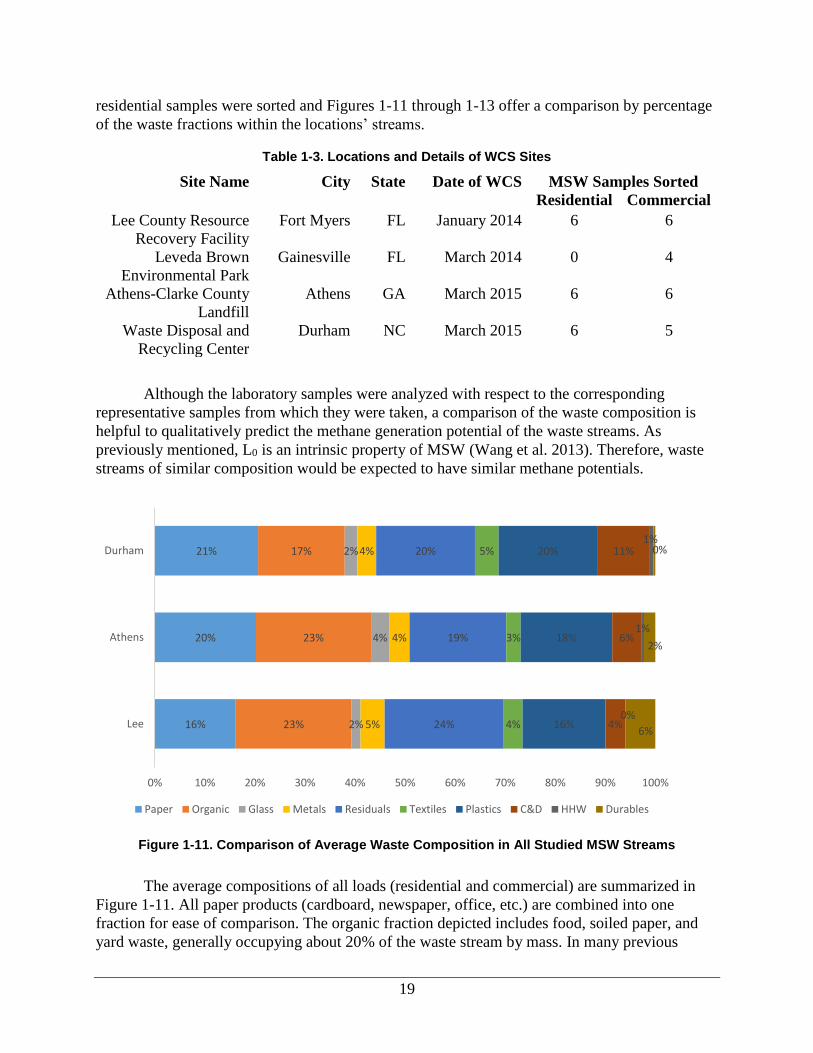
residential samples were sorted and Figures 1-11 through 1-13 offer a comparison by percentage
of the waste fractions within the locations’ streams.
Table 1-3. Locations and Details of WCS Sites
Site Name City State Date of WCS MSW Samples Sorted
Residential Commercial
Lee County Resource
Recovery Facility
Fort Myers FL January 2014 6 6
Leveda Brown
Environmental Park
Gainesville FL March 2014 0 4
Athens-Clarke County
Landfill
Athens GA March 2015 6 6
Waste Disposal and
Recycling Center
Durham NC March 2015 6 5
Although the laboratory samples were analyzed with respect to the corresponding
representative samples from which they were taken, a comparison of the waste composition is
helpful to qualitatively predict the methane generation potential of the waste streams. As
previously mentioned, L0 is an intrinsic property of MSW (Wang et al. 2013). Therefore, waste
streams of similar composition would be expected to have similar methane potentials.
Figure 1-11. Comparison of Average Waste Composition in All Studied MSW Streams
The average compositions of all loads (residential and commercial) are summarized in
Figure 1-11. All paper products (cardboard, newspaper, office, etc.) are combined into one
fraction for ease of comparison. The organic fraction depicted includes food, soiled paper, and
yard waste, generally occupying about 20% of the waste stream by mass. In many previous
16%
20%
21%
23%
23%
17%
2%
4%
2%
5%
4%
4%
24%
19%
20%
4%
3%
5%
16%
18%
20%
4%
6%
11%
0%
1%
1%
6%
2%
0%
0% 10% 20% 30% 40% 50% 60% 70% 80% 90% 100%
Lee
Athens
Durham
Paper Organic Glass Metals Residuals Textiles Plastics C&D HHW Durables

20
studies, the 20-25% of mass made up by the fines fractions was generally not investigated; the
time required to sort everything by hand in the field is substantial. The massive scale of landfills
and the large items found in MSW can make this fraction appear unimportant. The relatively
high methane potential of this material shows that this component is important to study. The
residuals fraction shown in Figure 1-11 includes both fines fractions, human and animal wastes,
and free liquids as collected, which ASTM D5231-92 would otherwise have roughly sorted into
“Other Organics” or “Other Inorganics” fractions that are indeterminable while sorting in the
field. The same data are shown in Figure 1-12 and Figure 1-13 with the results for residential and
commercial data, respectively.
The distribution of the fractions among sample sites is generally consistent, especially in
fractions with lower frequencies (glass, C&D, textiles). While plastic films only accounted for a
small fraction of the mass, in most loads this fraction occupied a large percentage of the volume.
C&D often accounted for a small fraction of the mass due to the truck selection method and the
presence of C&D facilities at or near the sampling locations. Even with the presence of C&D
facilities and electronic waste collection facilities, the relative mass of these materials (such as
wood, bricks, and metal) did account for some visible atypical values such as the larger C&D
fraction of Durham commercial waste and durables in Lee county, in which a few improperly
disposed heavy items changed the overall average.
Figure 1-12. Comparison of Average Waste Composition in Residential MSW Streams
12%
20%
16%
27%
24%
15%
2%
3%
3%
6%
5%
15%
24%
21%
27%
4%
3%
5%
14%
18%
15%
6%
4%
3%
0%
1%
1%
5%
1%
1%
0% 10% 20% 30% 40% 50% 60% 70% 80% 90% 100%
Lee
Athens
Durham
Paper Organic Glass Metals Residuals Textiles Plastics C&D HHW Durables

21
Figure 1-13. Comparison of Average Waste Composition in Commercial MSW Streams
1.10 Moisture Content and Volatile Solids Content of MSW Components
The moisture content and volatile solids content for each biodegradable component from
each representative sample was determined gravimetrically as described in Section 1.4.1. The
average values for each fraction are depicted in Figure 1-14 and Figure 1-15 for a visual
comparison to the other waste streams. Consistency among fractions from different sources, even
among samples that were collected under varying weather conditions, suggests sample sets were
large enough and the methodology was able to gather reproducible results.
Fractions such as textiles, wood, and yard waste showed more variation in average
moisture content, likely due to the reduced presence of these fractions among the selected loads
of MSW and the influence that individual samples can have (Appendix B. Moisture Content and
Volatile Solids Content Data). Note that composite wood was only sorted separately from
general wood (such as dimensional lumber) during the Lee County sort. The inconsistent
presence of each material led to the combination of both fractions in all future sorts. No wood of
any kind was found during the UF sorts at the Alachua Transfer Station. Additional spread in the
textile fractions could be attributed to the differences in natural and synthetic fibers as they were
sorted. Similar results are displayed for the volatile solids content (Figure 1-15). The
comparatively similar moisture content of the fines fractions was unexpected as these samples
should show the most heterogeneity of all fractions. The average moisture content of the Fines <
2” from Lee, Athens, and Alachua were all within a range of 5%.
20%
20%
23%
20%
19%
21%
16%
28%
1%
4%
1%
2%
4%
3%
9%
4%
24%
18%
11%
14%
3%
3%
5%
3%
19%
18%
17%
23%
2%
7%
18%
4%
0%
0%
1%
0%
7%
5%
0%
2%
0% 10% 20% 30% 40% 50% 60% 70% 80% 90% 100%
Lee
Athens
Durham
UF
Paper Organic Glass Metals Residuals Textiles Plastics C&D HHW Durables

22
Figure 1-14. Average Moisture Content of MSW Components Collected During WCS
Figure 1-15. Average VS/TS of MSW Components Collected During WCS
1.11 Volatile Solids Analysis of the Fines Fractions
The fines fractions were collected on site after falling through two different grids of
different size (2” and 1” square grid). Upon arrival in the SHWM laboratories, the fines fractions
were further sorted into organic and inorganic subfractions so that the methane contributing
fractions could be processed and assessed without interference from inert materials. This sorting
was done by hand on laboratory benches by manually removing bits of plastic, metals, and other
clearly inorganic materials prior to further analysis. Separating the inert fraction reduced wear on
grinding equipment and allowed better focus on the methane generating substances in the fines
fractions. This fraction was weighed and is identified as the “Removed Inorganic Fraction” in
Figure 1-16 and Figure 1-17. The remaining material was subjected to drying in a 105°C oven
0%
10%
20%
30%
40%
50%
60%
70%
Moisture Content
Lee
Athens
UF
Durham
0%10%20%30%40%50%60%70%80%90%
100%
Volatile Solids Content
Lee
Athens
UF
Durham

23
and combustion in a muffle furnace to determine the volatile solids (the “Volatile Organic
Fraction”) and non-volatile solids (the “Unremoved Inorganic Fraction”).
When reviewing the figures, it is evident that all 3 subfractions varied among the different
samples due to the inherent heterogeneous nature of the fines. Values of the Volatile Organic
Fraction range from as low as 5% to higher than 80% of the mass. The differences are due
mostly to the inability to perceive organic/inorganic components of soil-like materials that make
up a large mass of the fines fractions when hand sorting. The average composition of each
fraction is also presented in Table 1-4. It is important to note that the subsequent methane yield
experiments were performed only on the material that was perceived to be potentially
biodegradable during the benchtop sorting. The mass of the “Removed Inorganic Fraction” is
taken into calculation with the organic fraction yields when deriving the overall component
yields and determining L0. All yields for various fines composition data are listed in

24
Appendix C. Fines Composition Data.
Table 1-4. Summarized Composition of Fines Fractions by Mass
Fines < 2” Fines < 1”
Average Std. Dev Average Std. Dev
Volatile Organic Fraction 58% 13% 49% 19%
Unremoved Inorganic Fraction 15% 8% 22% 12%
Removed Inorganic Fraction 27% 14% 30% 23%
Figure 1-16. Composition of all Fines <2” Fractions
0%
10%
20%
30%
40%
50%
60%
70%
80%
90%
100%
Lee
Res
1
Lee
Res
2
Lee
Res
3
Lee
Res
4
Lee
Res
5
Lee
Res
6
Lee
Co
m 1
Lee
Co
m 2
Lee
Co
m 3
Lee
Co
m 4
Lee
Co
m 5
Lee
Co
m 6
Ath
ens
Res
1
Ath
ens
Res
2
Ath
ens
Res
3
Ath
ens
Res
4
Ath
ens
Res
5
Ath
ens
Res
6
Ath
ens
Co
m 1
Ath
ens
Co
m 2
Ath
ens
Co
m 3
Ath
ens
Co
m 4
Ath
ens
Co
m 5
Ath
ens
Co
m 6
Du
rham
Res
1
Du
rham
Res
2
Du
rham
Res
3
Du
rham
Res
4
Du
rham
Res
5
Du
rham
Res
6
Du
rham
Co
m 1
Du
rham
Co
m 2
Du
rham
Co
m 3
Du
rham
Co
m 4
Volatile Organic Fraction Unremoved Inorganic Fraction Removed Inorganic Fraction

25
Figure 1-17. Composition of all Fines <1” Fractions
1.12 Ultimate Methane Yields of MSW Components by BMP
The BMP assay is designed to determine the largest practical quantity of biogas that a
substrate can generate under ideal mesophilic conditions. A non-reactive color change oxygen
indicator, resazurin, is used to ensure strictly anaerobic conditions. A complex suite of anaerobes
generating methane at a strong rate is added to a nutrient broth that provides excess nutrients and
trace elements, leaving only the substrate being tested as the limiting factor. Over 1,500
individual BMP bottles were assembled and measured throughout the duration of this study,
providing over 10,000 data points that encompasses the predicted ranges of numerous past
published studies (Krause et al. 2016, 1117-1182).
A total of 14 OFMSW components were identified in this research and collected from
each representative sample at each facility. Laboratory samples were characterized by BMP and
analyzed in triplicate. As per the method, a control blank was included with each analysis to
consider methane generation from the existing organic material in the anaerobic broth. Thus,
these results are the net methane yield (i.e., measured – blank = net).
The box plot in Figure 1-18 shows the minimum, maximum, median, 1st quartile, and 3rd
quartile ranges of methane production in the BMP assays. For the purpose of reporting all
findings in this study, no data were excluded, and all data points are represented in this figure.
Appendix D. Distributions of Methane Yields by MSW Component shows histograms with the
average yield of every sample calculated by running triplicate bottles simultaneously. This same
approach was applied to gather the values in Table 1-5.
0%
10%
20%
30%
40%
50%
60%
70%
80%
90%
100%
Lee
Res
1
Lee
Res
2
Lee
Res
3
Lee
Res
4
Lee
Res
5
Lee
Res
6
Lee
Co
m 1
Lee
Co
m 2
Lee
Co
m 3
Lee
Co
m 4
Lee
Co
m 5
Lee
Co
m 6
Ath
ens
Res
1
Ath
ens
Res
2
Ath
ens
Res
3
Ath
ens
Res
4
Ath
ens
Res
5
Ath
ens
Res
6
Ath
ens
Co
m 1
Ath
ens
Co
m 2
Ath
ens
Co
m 3
Ath
ens
Co
m 4
Ath
ens
Co
m 5
Ath
ens
Co
m 6
Du
rham
Res
1
Du
rham
Res
2
Du
rham
Res
3
Du
rham
Res
4
Du
rham
Res
5
Du
rham
Res
6
Du
rham
Co
m 1
Du
rham
Co
m 2
Du
rham
Co
m 3
Du
rham
Co
m 4
Volatile Organic Fraction Unremoved Inorganic Fraction Removed Inorganic Fraction

26
Figure 1-18. Modified Box and Whisker Plots Represent Median Methane Yield From all Residential and Commercial MSW, 1st and 3rd Quartiles, and the Minimum and Maximum Values Measured
Accounting for non-gas-producing biological activity leads to confirmation that these
series produced reliable data. The low values of methane yield and tight spread of the blank
controls (those with no substrate added) further indicate successful repeatability and minimal
interference from the residual organic matter carried over from the anaerobic digester used to
culture methanogens. A summary of methane yield by fraction is shown in Table 1-5.
When reviewing these values in detail it can appear as if some values fall outside the
expected range. One newspaper sample from Durham produced a yield over three times the
average for other newspaper samples, while some food waste samples produced 25%-165% of
the mean yield for all food waste. Causes vary from paper products being saturated in grease to
high concentrations of dense indigestible fibers present in food waste. Similarly, inhibitory
substances can exist in products such as office paper that produce unexpectedly low yields. The
use of 450 samples run in triplicate during experimentation, paired with the minimum four times
that a sample was physically handled and inspected before making its way into a BMP bottle
reduced the margin of error when determining yields. The spread of values for more
heterogeneous samples such as food waste and the fines fractions is anticipated and the
consistency in previous MC and VS characterization lends support to the consistency and
accuracy of these methods.
0
100
200
300
400
500
600
mL
CH
4/g
VS
@ S
TP

27
Table 1-5. Range of Methane Yields by OFMSW Component (mL CH4/ g VS)
Fraction Average Methane Yield, 95%
Conf. Interval
Std.
Dev.
Min. Max. Median
Cardboard 216 ± 10 33 158 308 158
Newspaper 84 ± 21 62 18 322 18
Office Paper 293 ± 13 41 148 369 148
Pasteboard 233 ± 15 47 119 347 119
Junk Mail 281 ± 18 52 140 366 140
Aseptic Paper 255 ± 14 43 130 364 130
Misc. Paper 260 ± 19 60 98 367 98
Food and Soiled
Paper
328 ± 24 80 73 538 73
Yard Waste 137 ± 28 70 35 345 35
BF Fines <2” 318 ± 20 64 70 452 70
BF Fines <1” 322 ± 26 83 142 471 142
Textiles 214 ± 40 105 4 365 4
Wood 51 ± 15 40 9 171 9
Comp Wood 53 ± 23 37 16 132 16
Cellulose 332 ± 7 23 271 387 271
Blanks 7 ± 1 3 1 14 1
Note most the values in Table 1-5 are in proportion with past studies (e.g., office paper
yield > cardboard yield > newspaper yield) (Krause et al. 2016). These values were calculated
using the BMP data summarized in. An important finding is the high yield of the fines fractions,
which contributed between 19-26% of the average waste stream and averaged among the highest
yielding components. While the averages are comparable to past studies, the large number of
samples collected and analyzed for methane yield provided a broad range for some fractions. For
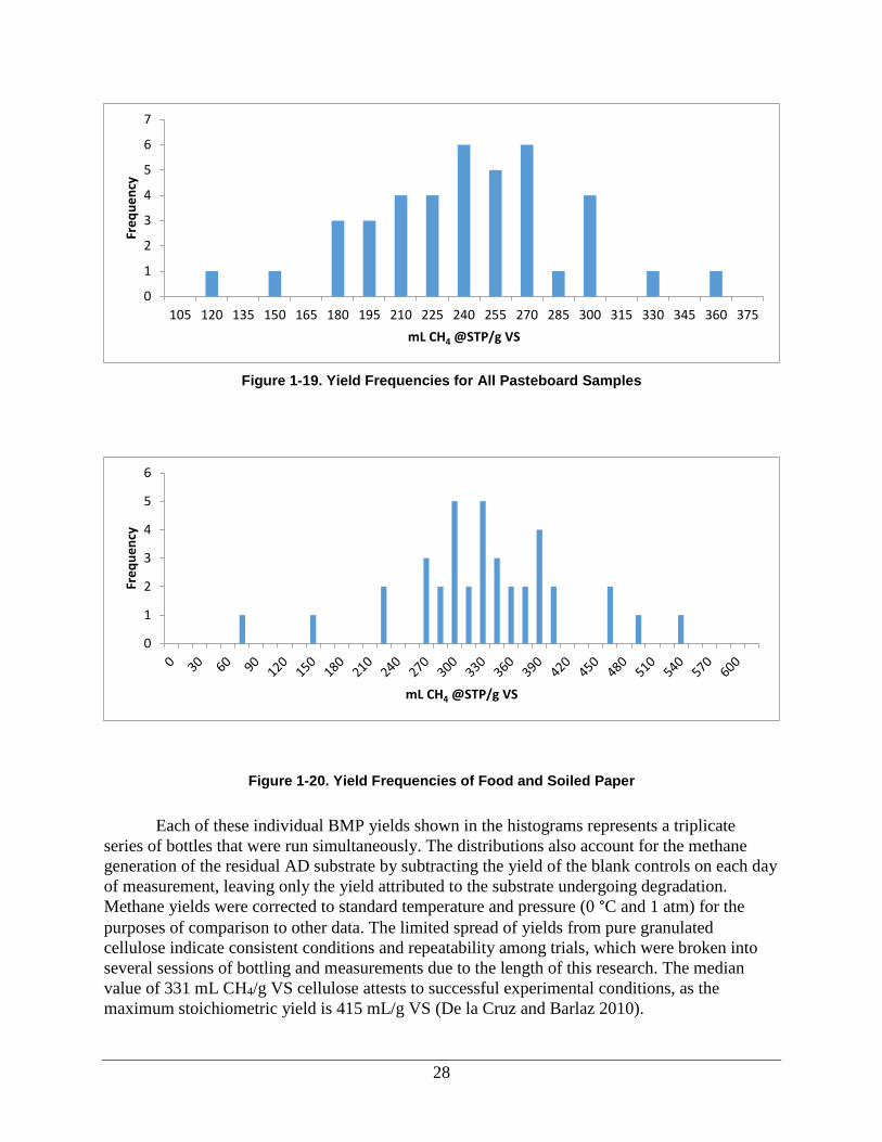
an example of this spread, refer to Figure 1-19 and Figure 1-20 or see all fractions depicted in
Appendix D. Distributions of Methane Yields by MSW Component.
28
Figure 1-19. Yield Frequencies for All Pasteboard Samples
Figure 1-20. Yield Frequencies of Food and Soiled Paper
Each of these individual BMP yields shown in the histograms represents a triplicate
series of bottles that were run simultaneously. The distributions also account for the methane
generation of the residual AD substrate by subtracting the yield of the blank controls on each day
of measurement, leaving only the yield attributed to the substrate undergoing degradation.
Methane yields were corrected to standard temperature and pressure (0 °C and 1 atm) for the
purposes of comparison to other data. The limited spread of yields from pure granulated
cellulose indicate consistent conditions and repeatability among trials, which were broken into
several sessions of bottling and measurements due to the length of this research. The median
value of 331 mL CH4/g VS cellulose attests to successful experimental conditions, as the
maximum stoichiometric yield is 415 mL/g VS (De la Cruz and Barlaz 2010).
0
1
2
3
4
5
6
7
105 120 135 150 165 180 195 210 225 240 255 270 285 300 315 330 345 360 375
Fre
qu
en
cy
mL CH4 @STP/g VS
0
1
2
3
4
5
6
Fre
qu
en
cy
mL CH4 @STP/g VS

29
Note that the spread of yield for pasteboard follows a relatively normal shape and has a
mean yield of 234 mL CH4/g VS and a median of 232. While the shape of the histograms for
some fractions does not appear bell-shaped every fraction passed a one sample Kolmogorov-
Smirnov test for normality using α = 0.05. For fractions like food and soiled paper (Figure 1-20)
that are substantially more heterogeneous, the distribution is much wider, though the data still
manage to form a mostly normal shape with only three points that appear abnormal (two high,
one low) of the 39 collected food and soiled paper samples. No data were excluded in this report
under the assumption that consistent yields in triplicate samples (which all these samples
showed) was indicative of successful experimentation. Comparatively high or low yields were
checked for clerical errors prior to reporting and all values presented are authentic
measurements.
For the purpose of comparing the yields of the individual components of MSW with
different models of assessing methane yield in landfills,
Table 1-6. Comparison of Methane Yields in Dry and As-Discarded Form 1-6 shows the
comparison of the yields determined for the dry samples and the respective yields expected per
mass unit of each fraction as it arrives at a waste disposal site. These values were calculated by
applying the average moisture content and volatile solids content to the mean yield of each
fraction. The difference in yield when factoring in moisture content reduces the yield per unit
mass for food and yard waste by approximately 50% and highlights how much moisture
contamination can reduce the yield of materials such as office paper.
Table 1-6. Comparison of Methane Yields in Dry and As-Discarded Form
Fraction MC VS Dry Yield (mL
CH4/g VS)
As-Discarded
Yield (m3
CH4/Mg MSW)
Cardboard 22% 88% 216 148
Newspaper 25% 90% 84 57
Office Paper 19% 81% 293 194
Pasteboard 17% 77% 233 148
Junk Mail 22% 85% 281 186
Aseptic Paper 20% 80% 255 163
Misc. Paper 23% 95% 260 191
Food and Soiled
Paper
50% 91% 328 149
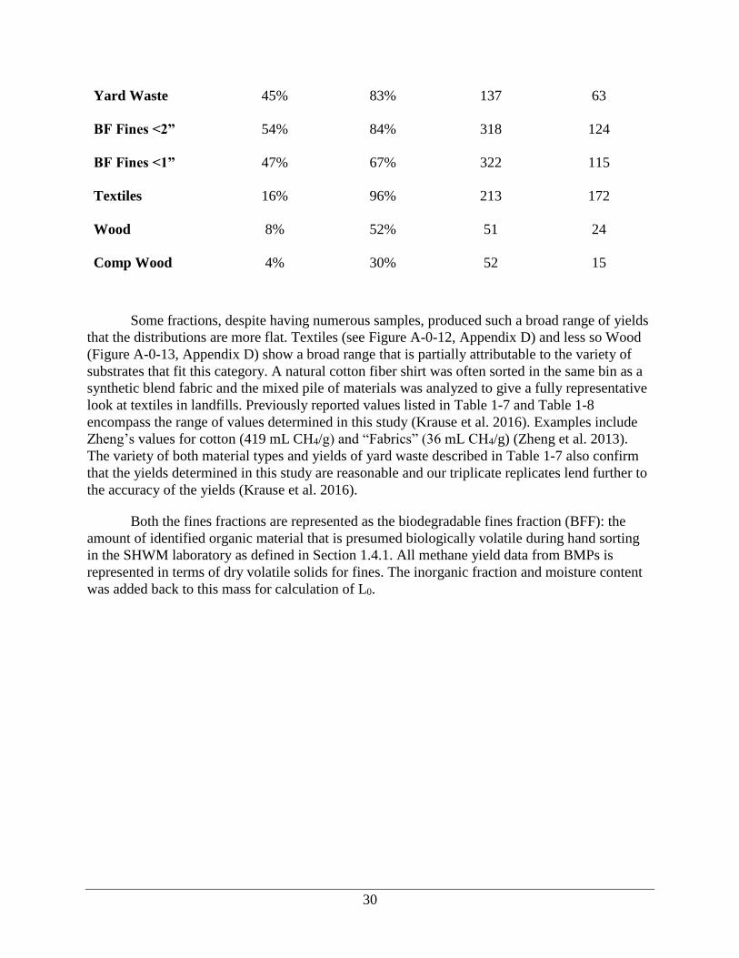
30
Yard Waste 45% 83% 137 63
BF Fines <2” 54% 84% 318 124
BF Fines <1” 47% 67% 322 115
Textiles 16% 96% 213 172
Wood 8% 52% 51 24
Comp Wood 4% 30% 52 15
Some fractions, despite having numerous samples, produced such a broad range of yields
that the distributions are more flat. Textiles (see Figure A-0-12, Appendix D) and less so Wood
(Figure A-0-13, Appendix D) show a broad range that is partially attributable to the variety of
substrates that fit this category. A natural cotton fiber shirt was often sorted in the same bin as a
synthetic blend fabric and the mixed pile of materials was analyzed to give a fully representative
look at textiles in landfills. Previously reported values listed in Table 1-7 and Table 1-8
encompass the range of values determined in this study (Krause et al. 2016). Examples include
Zheng’s values for cotton (419 mL CH4/g) and “Fabrics” (36 mL CH4/g) (Zheng et al. 2013).
The variety of both material types and yields of yard waste described in Table 1-7 also confirm
that the yields determined in this study are reasonable and our triplicate replicates lend further to
the accuracy of the yields (Krause et al. 2016).
Both the fines fractions are represented as the biodegradable fines fraction (BFF): the
amount of identified organic material that is presumed biologically volatile during hand sorting
in the SHWM laboratory as defined in Section 1.4.1. All methane yield data from BMPs is
represented in terms of dry volatile solids for fines. The inorganic fraction and moisture content
was added back to this mass for calculation of L0.

31
Table 1-7. Methane Generation Parameters of Wood Products and Yard Waste
Yard waste and
wood products
Moisture
Content
(% w/w)
Volatile
Solids
(% of TS)
Methane Yield Methane
Generation
Potential
Reference
mL/g
VS
m3/Mg
dry
L0
(m3 CH4/ Mg
wet)
Branch
96.6
63
(Eleazer et al. 1997)
Branches
134
(Owens and
Chynoweth 1993)
Garden waste
114
(Trzcinski and
Stuckey 2011)
Grass 68.9 86 388 334* 104* (Buffiere et al.
2006)
Grass
209
(Owens and
Chynoweth 1993)
Grass
85.0
144
(Eleazer et al. 1997)
Grass-2
87.8
128
(Eleazer et al. 1997)
Hardwoods
0 -
32.5
(Wang et al. 2011)
Leaves
123
(Owens and
Chynoweth 1993)
Leaves
90.2
31
(Eleazer et al. 1997)
Medium-
density
Fiberboard
4.6
(Wang et al. 2011)
Oriented strand
board
0 -
84.5
(Wang et al. 2011)
Particleboard
5.6
(Wang et al. 2011)
Plywood
6.3
(Wang et al. 2011)
Softwoods
0.5 -
7.5
(Wang et al. 2011)
Wood
100 193 193
(Cho, Moon, and
Kim 2012)
Yard waste
5 - 9
(O'Keefe et al. 1993)
Yard waste
143
(Owens and
Chynoweth 1993) *Calculated based on reported characterization data including moisture content, total solids, or volatile solids content.
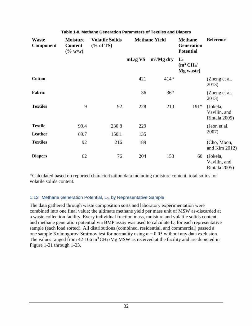
32
Table 1-8. Methane Generation Parameters of Textiles and Diapers
Waste
Component
Moisture
Content
(% w/w)
Volatile Solids
(% of TS)
Methane Yield Methane
Generation
Potential
Reference
mL/g VS m3/Mg dry L0
(m3 CH4/
Mg waste)
Cotton
421 414*
(Zheng et al.
2013)
Fabric
36 36*
(Zheng et al.
2013)
Textiles 9 92 228 210 191* (Jokela,
Vavilin, and
Rintala 2005)
Textile 99.4 230.8 229
(Jeon et al.
2007) Leather 89.7 150.1 135
Textiles 92 216 189 (Cho, Moon,
and Kim 2012)
Diapers 62 76 204 158 60 (Jokela,
Vavilin, and
Rintala 2005)
*Calculated based on reported characterization data including moisture content, total solids, or
volatile solids content.
1.13 Methane Generation Potential, L0, by Representative Sample
The data gathered through waste composition sorts and laboratory experimentation were
combined into one final value; the ultimate methane yield per mass unit of MSW as-discarded at
a waste collection facility. Every individual fraction mass, moisture and volatile solids content,
and methane generation potential via BMP assay was used to calculate L0 for each representative
sample (each load sorted). All distributions (combined, residential, and commercial) passed a
one sample Kolmogorov-Smirnov test for normality using α = 0.05 without any data exclusion.
The values ranged from 42-166 m3 CH4 /Mg MSW as received at the facility and are depicted in
Figure 1-21 through 1-23.
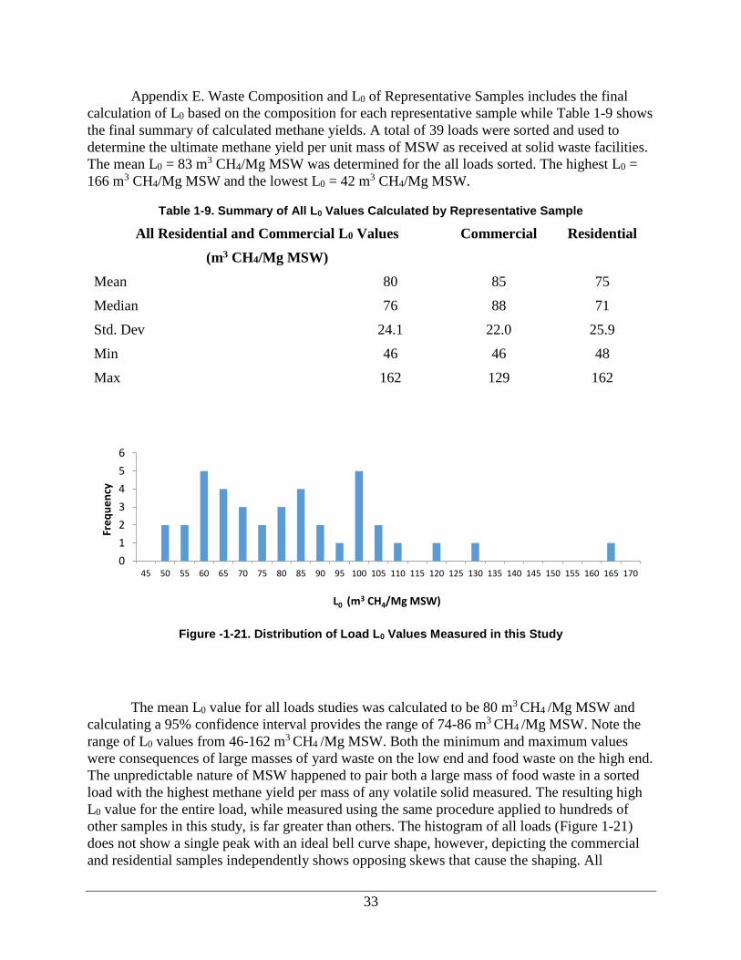
33
Appendix E. Waste Composition and L0 of Representative Samples includes the final
calculation of L0 based on the composition for each representative sample while Table 1-9 shows
the final summary of calculated methane yields. A total of 39 loads were sorted and used to
determine the ultimate methane yield per unit mass of MSW as received at solid waste facilities.
The mean L0 = 83 m3 CH4/Mg MSW was determined for the all loads sorted. The highest L0 =
166 m3 CH4/Mg MSW and the lowest L0 = 42 m3 CH4/Mg MSW.
Table 1-9. Summary of All L0 Values Calculated by Representative Sample
All Residential and Commercial L0 Values
(m3 CH4/Mg MSW)
Commercial Residential
Mean 80 85 75
Median 76 88 71
Std. Dev 24.1 22.0 25.9
Min 46 46 48
Max 162 129 162
Figure -1-21. Distribution of Load L0 Values Measured in this Study
The mean L0 value for all loads studies was calculated to be 80 m3 CH4 /Mg MSW and
calculating a 95% confidence interval provides the range of 74-86 m3 CH4 /Mg MSW. Note the
range of L0 values from 46-162 m3 CH4 /Mg MSW. Both the minimum and maximum values
were consequences of large masses of yard waste on the low end and food waste on the high end.
The unpredictable nature of MSW happened to pair both a large mass of food waste in a sorted
load with the highest methane yield per mass of any volatile solid measured. The resulting high
L0 value for the entire load, while measured using the same procedure applied to hundreds of
other samples in this study, is far greater than others. The histogram of all loads (Figure 1-21)
does not show a single peak with an ideal bell curve shape, however, depicting the commercial
and residential samples independently shows opposing skews that cause the shaping. All
0
1
2
3
4
5
6
45 50 55 60 65 70 75 80 85 90 95 100 105 110 115 120 125 130 135 140 145 150 155 160 165 170
Fre
qu
en
cy
L0 (m3 CH4/Mg MSW)

34
distributions (combined, residential, and commercial) passed a one sample Kolmogorov-Smirnov
test for normality using α = 0.05 and were considered acceptable without any data exclusion.
Figure 1-22. Frequency and Range of all L0 Values Measured from Commercial Samples
Figure 1-22 is a histogram of the L0 values determined for commercial loads only. The
data mildly skew left while illustrating data with a mean value of 85 m3 CH4 /Mg MSW and a
median value of 88. Calculating a 95% confidence interval provides the range of 77-92 m3 CH4
/Mg MSW for all commercial loads. These values are relatively proportional in opposition to the
residential data in Figure 1-23 which shows data skewing to the right and a lower mean L0 = 75
m3 CH4 /Mg MSW and median 71, as well as a 95% confidence interval provides the range of
67-85 m3 CH4 /Mg MSW. With the exception of the single high value (due to the uncommonly-
high amount of methane-generating food waste in the sample) the residential data hold a more
concentrated spread than the commercial loads. While the histograms suggest a difference
between the two groups, a two-sample t test with alpha = 0.05 showed no significant difference
between commercial and residential L0 values. Similar t tests between different counties showed
no significant difference in L0 related to source region.
Figure 1-23. Frequency and Range of All L0 Values Measured from Residential Samples
0
1
2
3
4
5
50 60 70 80 90 100 110 120 130 140
Fre
qu
en
cy
L0 (m3 CH4/Mg MSW)
0
1
2
3
4
45 50 55 60 65 70 75 80 85 90 95 100 105 110 115 120 125 130 135 140 145 150 155 160 165 170
Fre
qu
en
cy
L0 (m3 CH4/Mg MSW)
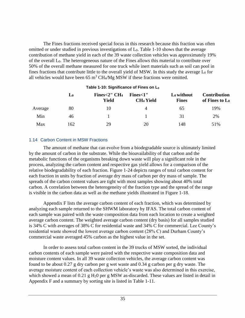
35
The Fines fractions received special focus in this research because this fraction was often
omitted or under studied in previous investigations of L0. Table 1-10 shows that the average
contribution of methane yield in each of the 39 waste collection vehicles was approximately 19%
of the overall L0. The heterogeneous nature of the Fines allows this material to contribute over
50% of the overall methane measured for one truck while inert materials such as soil can pool in
fines fractions that contribute little to the overall yield of MSW. In this study the average L0 for
all vehicles would have been 65 m3 CH4/Mg MSW if these fractions were omitted.
Table 1-10: Significance of Fines on L0
L0 Fines<2" CH4
Yield
Fines<1"
CH4 Yield
L0 without
Fines
Contribution
of Fines to L0
Average 80 10 4 65 19%
Min 46 1 1 31 2%
Max 162 29 20 148 51%
1.14 Carbon Content in MSW Fractions
The amount of methane that can evolve from a biodegradable source is ultimately limited
by the amount of carbon in the substrate. While the bioavailability of that carbon and the
metabolic functions of the organisms breaking down waste will play a significant role in the
process, analyzing the carbon content and respective gas yield allows for a comparison of the
relative biodegradability of each fraction. Figure 1-24 depicts ranges of total carbon content for
each fraction in units by fraction of average dry mass of carbon per dry mass of sample. The
spreads of the carbon content values are tight with most samples showing about 40% total
carbon. A correlation between the heterogeneity of the fraction type and the spread of the range
is visible in the carbon data as well as the methane yields illustrated in Figure 1-18.
Appendix F lists the average carbon content of each fraction, which was determined by
analyzing each sample returned to the SHWM laboratory by IFAS. The total carbon content of
each sample was paired with the waste composition data from each location to create a weighted
average carbon content. The weighted average carbon content (dry basis) for all samples studied
is 34% C with averages of 38% C for residential waste and 34% C for commercial. Lee County’s
residential waste showed the lowest average carbon content (28% C) and Durham County’s
commercial waste averaged 45% carbon as the highest value in the set.
In order to assess total carbon content in the 39 trucks of MSW sorted, the individual
carbon contents of each sample were paired with the respective waste composition data and
moisture content values. In all 39 waste collection vehicles, the average carbon content was
found to be about 0.27 g dry carbon per g wet waste and 0.34 g carbon per g dry waste. The
average moisture content of each collection vehicle’s waste was also determined in this exercise,
which showed a mean of 0.21 g H20 per g MSW as-discarded. These values are listed in detail in
Appendix F and a summary by sorting site is listed in Table 1-11.

36
Figure 1-24. Total Carbon Content (Dry Mass Carbon/Dry Mass Material) by Fraction. Boxes Show Median, 1st and 3rd Quartiles of the Data for Each Fraction (Whiskers Represent Minimum and
Maximum Values)
Table 1-11. Total Carbon Content by Fraction (Dry Mass Carbon/Dry Mass Sample)
Average Carbon Content Std. Dev Min Max
Cardboard 42% 2% 35% 45%
Newspaper 45% 3% 36% 53%
Office Paper 38% 2% 35% 45%
Pasteboard 40% 1% 37% 45%
Junk Mail 36% 3% 29% 45%
Aseptic Paper 45% 2% 42% 49%
Misc. Paper 38% 3% 32% 45%
Food and Soiled Paper 43% 5% 30% 62%
Yard Waste 42% 5% 26% 47%
BF Fines <2" 40% 4% 33% 50%
BF Fines <1" 37% 8% 15% 54%
Textiles 47% 10% 40% 92%
Wood 44% 2% 39% 46%
Comp. Wood 41% 2% 38% 44%
0%
10%
20%
30%
40%
50%
60%
70%
80%
90%
100%
Ave
rage
% T
ota
l Car
bo
n, d
ry b
asis
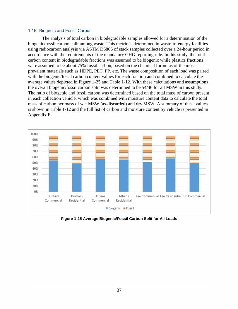
37
1.15 Biogenic and Fossil Carbon
The analysis of total carbon in biodegradable samples allowed for a determination of the
biogenic/fossil carbon split among waste. This metric is determined in waste-to-energy facilities
using radiocarbon analysis via ASTM D6866 of stack samples collected over a 24-hour period in
accordance with the requirements of the mandatory GHG reporting rule. In this study, the total
carbon content in biodegradable fractions was assumed to be biogenic while plastics fractions
were assumed to be about 75% fossil carbon, based on the chemical formulas of the most
prevalent materials such as HDPE, PET, PP, etc. The waste composition of each load was paired
with the biogenic/fossil carbon content values for each fraction and combined to calculate the
average values depicted in Figure 1-25 and Table 1-12. With these calculations and assumptions,
the overall biogenic/fossil carbon split was determined to be 54/46 for all MSW in this study.
The ratio of biogenic and fossil carbon was determined based on the total mass of carbon present
in each collection vehicle, which was combined with moisture content data to calculate the total
mass of carbon per mass of wet MSW (as-discarded) and dry MSW. A summary of these values
is shown in Table 1-12 and the full list of carbon and moisture content by vehicle is presented in
Appendix F.
Figure 1-25 Average Biogenic/Fossil Carbon Split for All Loads
0%
10%
20%
30%
40%
50%
60%
70%
80%
90%
100%
DurhamCommercial
DurhamResidential
AthensCommercial
AthensResidential
Lee Commercial Lee Residential UF Commercial
Biogenic Fossil

38
Table 1-12. Average Biogenic/Fossil Carbon Split for All Loads. Based on Dry Mass Carbon/Dry Mass Waste Composition
Biogenic Carbon Fossil Carbon Total Carbon (g
C/g dry MSW)
Total Carbon (g
C/g wet MSW)
Durham Commercial 54% 46% 45% 33%
Durham Residential 49% 51% 37% 27%
Athens Commercial 56% 44% 33% 27%
Athens Residential 56% 44% 33% 26%
Lee Commercial 51% 49% 30% 25%
Lee Residential 58% 42% 26% 22%
UF Commercial 50% 50% 41% 31%
Average 54% 46% 34% 27%
Figure 1-26. Comparison of L0 and Biogenic Carbon Content for each Load, Dur-Com 3 Excluded
Total carbon content for each sample was applied with the waste composition data to
determine the biogenic/fossil carbon content. Figure 1-26 shows a comparison of the methane
yield (L0) of each load sorted and the biogenic carbon content (wet weight) for each respective
load. This figure’s regression line excludes the L0 value for Durham Commercial 2 (shown in
red), which was relatively low (46 m3 CH4/Mg MSW) as a result of uncommonly-high presence
y = 480.39x + 12.352R² = 0.366
0
20
40
60
80
100
120
140
160
180
0.000 0.050 0.100 0.150 0.200 0.250
L 0(m
3C
H4/M
g M
SW a
s-d
isca
rded
)
Biogenic Carbon Content- Wet (g biogenic C /g wet waste)

39
of wood (52% of as-discarded mass) in the load. Excluding this L0 value increased the
percentage of variation explained by the linear model from about 20% to nearly 37%. Regression
analysis based on 95% confidence intervals revealed a statistically significant relationship
between biogenic carbon content (wet weight) and L0 for the data sets inclusive (P-value = 5.7 x
10-5) and excluding (P-value = 4 x 10⁻³) of Durham Commercial 2. A table of these values is
located in Appendix F.
The fines fractions received specific interest because of the difficulty in characterizing
the material. Table 1-13 lists the samples used and shows that no correlation between yield and
biogenic carbon content was defined for the fines fractions. The carbon in these samples was
almost completely biogenic. The fractions analyzed by Beta Analytic had been hand sorted to
remove items that were perceived as non-biodegradable (the Inert Fines Fraction described in
Section 2.4.1) which accounted for between 13% and 59% of the mass. A small amount of
plastic films were removed in this process- less than 10% of the removed mass. The majority of
IFF material removed was glass shards, rocks/pebbles, cigarettes, and clay cat litter. The plastics
that could have contributed fossil carbon to the samples were minimal in mass relative to heavy
items such as soil and food waste that made up a majority of the composition. See Appendix C
for more composition data of the fines fractions. No correlation between BFF size and biogenic
carbon content was observed in the samples studied.
Table 1-13. Biogenic Carbon Content in Dry, Ground, Sorted Biodegradable Fines Fractions
County Load Fraction CH4 Yield
(mL/g
VS)
Biogenic Carbon
Content in Dry
Samples (percent
modern carbon)
Biodegradable Fines Fraction
(wet mass of fines sample
kept/wet mass of total fines
sample before sorting)
Lee Res 6 BF<2" 289 99% 61%
Lee Com 6 BF<2" 318 100% 41%
Durham Com 3 BF<2" 353 99% 75%
Athens Com 3 BF<1" 283 100% 87%
Athens Res 2 BF<1" 324 100% 65%
Durham Res 5 BF<1" 366 100% 75%
1.16 Degradable Carbon Fraction
By calculating each yield of methane and carbon dioxide at STP, the density of each gas
under standard conditions was used to determine the fraction of carbon in each sample that
evolved to either gas. Figure 1-27 portrays how carbon was studied and described in this research
with total carbon assessed as described in Section 3.6. The biogenic/fossil carbon split detailed in
Section 3.7 is describing the physical makeup of the total carbon content. The amount of
biogenic carbon that evolved into carbon in CO2 or CH4 was determined by assessing the yields
of gas and comparing the respective yield for each sample to the amount of biogenic carbon
present prior to digestion under anaerobic conditions. In all waste samples studied the average
fraction of biogenic carbon mass that evolved to carbon in CO2 and CH4 was 43%. Commercial
carbon averaged 47% and residential carbon averaged 51%. Individual sites are listed in
Table 1-14 and range from 38-53%. The biogenic carbon mass fractions determined for
residential and commercial fractions of MSW from Lee County of 52% and 50% for commercial

40
and residential waste respectively. These values are less than those reported to the U.S. EPA by
the Lee County Solid Waste Resource Recovery Facility (RRF), which were reported to be
64.3% when measured in facility’s emissions stream (U.S. EPA 2013). The RRF collects
quarterly 24-hour stack samples for radiocarbon analysis to ascertain the fraction of carbon that
is biogenic in origin to meet EPA requirements. From 2014 to 2016, these quarterly samples
ranged from 59% to 63% biogenic carbon (U.S. EPA 2016).
Figure 1-27. Carbon Studied in this Research
Table 1-14. Average Degradable Carbon Fraction by Location. Values Represent % of Dry Mass of Total Biogenic Carbon that Evolved to Carbon in CH4 or CO2
Location Average Fraction of Biogenic
Carbon Evolved to Carbon
in Biogas (CH4 and CO2)
Durham Commercial 38%
Durham Residential 50%
Athens Commercial 48%
Athens Residential 53%
Lee Commercial 50%
Lee Residential 52%
UF Commercial 52%
The average content of degradable carbon was determined after the values were
determined for each individual sample. Figure 1-28 shows the spread of all degradable carbon

41
percentages, grouped by fraction. Similar to the methane yields show in shown in Figure 1-28,
increased heterogeneity in the sample results in a wider spread of values. High lignin content in
fibrous materials such as newspaper, wood, and yard waste is known to reduce methane yields
under anaerobic conditions, as the carbon is not easily available to these organisms without prior
hydrolysis. While wood and newspaper both have average carbon contents of 45%, only 9% and
5%, respectively, of that carbon was able to convert to both CO2 and CH4 in the BMP assays.
The maximum value for newspaper, illustrated with the whiskers in Figure 1-28 is likely due to
contamination such as oil or sugar saturating the newspaper prior to study.
Table 1-15 presents the mean values of this degradable carbon by fraction and displays the
average fraction of carbon that evolved to CO2 and CH4 for comparison. The ratio of C evolved to
CH4 to C evolved to CO2 ranged from 1.1 (office paper) to 2.4 (newspaper). Typical anaerobic
landfill gas exhibits CH4 to CO2 ratios in the range of 1.0 to 1.5 (anaerobic bioconversion of
cellulose results in a theoretical ratio of 1.0). As some CO2 will dissolve into solution in the BMP
bottle, the amount of CO2 measured is expected to be less than that produced. This effect is
magnified for those constituents with lower methane yields (e.g., wood, newspaper). In addition,
those constituents with greater amounts on non-cellulosic biodegradable organic matter (e.g., food
waste, fines), also results in higher CH4 to CO2 ratios, not surprising, as fats and lipids yield a
greater percentage of CH4 compared to cellulosic materials.
Figure 1-28. Percent of Total Carbon Evolved to Both CH4 and CO2 by Component. Boxes Show Median, 1st and 3rd Quartiles of the Data for Each Fraction. Whiskers Represent Minimum and Maximum Values. Values Represent % of Dry Mass of Total Biogenic Carbon that Evolved to
Carbon in CH4 or CO2
0%
10%
20%
30%
40%
50%
60%
70%
80%
90%
100%
% T
ota
l Car
bo
n E
vole
d t
o C
H4
& C
O2

42
Table 1-15. Average Degradable Carbon Fraction by Fraction. Values Represent Average % of Total Carbon (Mass) in Dry Samples that Evolved to Carbon in CH4 or CO2
Fraction Average Fraction
of Carbon that
Evolved to C in
CH4
Average Fraction
of Carbon that
Evolved to C in
CO2
Ratio of fraction C
evolved to C in
CH4: fraction C
evolved to C in
CO2
Cardboard 25% 14% 1.8
Newspaper 10% 4% 2.4
Office Paper 29% 27% 1.1
Pasteboard 29% 22% 1.3
Junk Mail 36% 30% 1.2
Aseptic Paper 29% 21% 1.4
Misc. Paper 29% 23% 1.3
Food and Soiled Paper 35% 22% 1.6
Yard Waste 15% 9% 1.7
BF Fines <2” 32% 18% 1.8
BF Fines <1” 31% 17% 1.8
Textiles 25% 19% 1.4
Wood 5% 3% 1.8
Comp Wood 7% 4% 2.0

43
Conclusions
Waste composition studies were employed to capture MSW from waste collection
vehicles at the point of disposal to ensure that the maximum amount of degradable materials
remained intact for laboratory analysis. Representative samples were identified and sorted
following ASTM D5231-92 and organic fractions were returned to the UF Environmental
Engineering Laboratories for further study. Laboratory analyses were used to characterize the
biodegradable components with respect to methane generation via BMP assay. Methane
generation data were then attributed to the weight-fraction of the component determined in the
WCS and L0 for each representative sample was determined.
L0 values were found to range from 46-162 m3 CH4/Mg MSW, with an average value of
80 m3/Mg MSW (Table 1-9). While the geographic range covered by the samples does not
represent the entire U.S. it does provide insight on L0 based on the analysis of as-discarded
commercial and residential MSW. The L0 values for the 39 MSW collection vehicle samples
gathered during this study were normal in distribution as tested by a one sample Kolmogorov-
Smirnov test for normality using α = 0.05. This suggested that waste composition and laboratory
analysis yielded consistent results among samples obtained from different locations with the
process developed for this study.
This average value is 20% lower than the current 100 m3 CH4/Mg MSW value for L0
suggested by the USEPA in AP-42; however, the range of values does not exclude a value of 100
m3 CH4/Mg MSW from the range of possibilities. Of the 39 trucks sorted, six resulted in L0
values higher than 100, one of which produced a calculated 162 m3 CH4/Mg MSW-nearly as
much as the potential to emit factor of 170 m3 CH4/Mg MSW required for use by the landfill new
source performance standards and emissions guidelines promulgated under the Clean Air Act.
Twelve of the 39 trucks sorted produced L0 values between the average 80 and 100 m3 CH4/Mg
MSW.
The methane evolved from these samples originated from biogenic carbon found in the
waste. The solid waste in this study showed an average total carbon content on a dry basis of
34%. Of that total carbon, 54% was estimated to be biogenic carbon and 46% was estimated to
be fossil carbon. The average fraction of biogenic carbon that evolved to CH4 or CO2 is 43%. If
100 kg of waste with an average composition is placed in one of the landfills that hosted a waste
sort in this study, 11.8 kg of carbon is expected to be converted to biogas at STP.
The range of L0 values found in this study can be attributed to the 450 samples, the
heterogeneous nature of the MSW, and the need to categorize waste samples into manageable
categories for study. The clear differences between residential and commercial waste yields and
the varying proportions in which they could be received leads one to conclude that the source of
waste and the varying compositions will have a significant impact on the ultimate yield of
landfilled materials. Since these wastes are all managed the same way in landfills the results
were combined as presented in this work. The results from this study do fall within the range
reported with similar BMP studies; Figure 1-29 depicts these values, all of which were
determined using different methods, reactor sizes, and substantially smaller sample sets.

44
Figure 1-29. Comparison of Past Studies of L0
The average of these other studies is 89.8 m3 CH4/Mg MSW (some of which had to be
calculated using their reported VS and MC values), and the entire range of L0 values determined
in this study is found within the confines of these previously published reports. While this is not
a complete list of published L0 values, these numbers were determined in studies around the
world and a large set of samples obtained in the southeastern United States was able to verify
that nearly all previous values were within predictable ranges and able to be reproduced using
MSW collected at the point of disposal.
The intent of the current study was not to develop a nationwide L0 value for MSW but
rather to provide insight as to how the L0 of current residential and commercial MSW compares
to the AP-42 default and other studies. Such information should prove beneficial to those who
rely on the FOD models for landfill gas production.
As a short exercise, to determine if uncommonly large or small yields of individual
components were impacting the average yields presented in this report, all BMP values for each
of the 39 trucks sorted were replaced with the average values reported in Table 1-5. The L0
values determined through this exercise are shown in Figure 1-30 and form a more qualitatively
perfect bell curve shape, though both this calculated L0 set and that which was determined with
the fractions measured for methane yield both pass for normality. While the actual data produces
a qualitatively less perfect shape, the distribution did pass a one sample Kolmogorov-Smirnov
test for normality using α = 0.05 and was considered acceptable without any data exclusion. No
data was excluded from any of the findings presented in this report.
0
20
40
60
80
100
120
140
160
180
200L 0
(m3
CH
4/ M
g M
SW)

45
Figure 1-30. Frequency and Range of All L0 Values Calculated Using Average Yields for each Individual Organic Fraction
The visual representation is slightly misleading in this case as the average values vary
little between the individual L0 values and those determined with average yields for each organic
fraction. These values are compared in Table 1-16. While the histograms suggest a difference
between the L0 values of the two groups, a two-sample t test with alpha = 0.05 showed no
significant difference.
Table 1-16. Comparison of L0 Values Calculated Using Average Yields and Individualized Yields for Each Individual Organic Fraction
L0 Values Determined with
Individual Yields (Figure 1-21)
L0 Values Determined with
Average Yields (Figure 1-30)
Mean 80 84
Median 76 81
Std. Dev 24.1 18.7
Min 46 48
Max 162 131
While the range of methane yields for each fraction of MSW could vary, much of the
variation could be attributed to heterogeneity in the fraction (e.g., food wastes, fines), unique
characteristics of different manufactured products (e.g., lignin content in newspaper and
cardboard), or unavoidable contamination of liquids on dry materials. From the 39 representative
samples collected in this study, over 1,400 BMPs were performed on the 14 biodegradable waste
fractions, analyzed in triplicate.
In addition to determining them methane potential for these samples, further investigation
into the physical characteristics provides us with a better understanding of waste today. For each
01234567
45 50 55 60 65 70 75 80 85 90 95 100 105 110 115 120 125 130 135 140
Fre
qu
en
cy
L0 (m3 CH4/Mg MSW)
46
sample studied in one contained research effort, we know its source, prevalence relative to the
truck from which it was pulled, the county in which it originated, and how its presence rates
relative to other samples from three different states. We also know the moisture and volatile
solids content of that specific sample, as well as the total carbon content. The methane and
carbon dioxide potentials were determined on that same mass of waste that was sorted hundreds
of miles away. After determining the carbon content of that sample, the fraction of molecules
that are capable of changing phases from solid to gas under anaerobic conditions was also
determined. This same chain of investigation was carried out 450 times in this research. A
comparison of the biogenic carbon content and L0 values revealed that the biogenic carbon
content/wet mass of as-discarded MSW can account for approximately 37% of the variation in
measured methane potential.
The objective of this research was to measure the L0 of both residential and commercial
MSW in the condition and composition at the point of disposal. This work was motivated by
recent studies that suggest the actual MSW L0 values are substantially lower than the current AP-
42 default values of 100 m3 CH4/Mg MSW. L0 values were found in this work resulted in a range
from 46-162 m3 CH4/Mg MSW, with an average value of 80 m3/Mg MSW. While the average
value found here is less than the AP-42 default value, the AP-42 default was within the range of
values determined in this study. Differences between the results found in this study and other
work stems from the contribution of waste materials outside the typical stream of household and
commercial MSW going to landfills (some of which are accounted for in waste composition
studies) and include items such as soil, sludge, and building debris. This study also measured
methane potential of all biodegradable waste components including the miscellaneous, or
“Fines” fractions were found to contribute an average of 19% of the total methane yield for each
load of MSW studied. In one load the fines contributed over 50% of the total methane generated.
If fines were omitted from this study completely, the average L0 calculated would have been 65
m3 CH4/Mg MSW as opposed to 80. While the limited geographic extent covered here precludes
describing these results as representative of nationwide MSW, they should provide context to
those utilizing L0 in FOD projections.

47
References
Amini H, Reinhart D, Niskanen A. 2013. “Comparison of first-order-decay modeled and actual
field measured municipal solid waste landfill methane data.” Waste Management,
Elsevier Ltd. 33(12):2720-2728.
Amini H, Reinhart D, Mackie K. 2012. “Determination of first-order landfill gas modeling
parameters and uncertainties.” Waste Management, Elsevier Ltd. 32(2):305-316.
APHA. 1999. “2540 SOLIDS.” Standard Methods for The Examination of Water and
Wastewater. American Public Health Association, American Water Works Association,
Water Environment Federation.
ASTM International. 2016. “ASTM D5231-92(2016) Standard Test Method for Determination of
the Composition of Unprocessed Municipal Solid Waste.” ASTM International, West
Conshohocken, PA, USA.
ASTM International. 2009. “ASTM D2974-07a Standard Test Method for Moisture, Ash, and
Organic Matter of Peat and Other Organic Soils.” ASTM International, West
Conshohocken, PA, USA.
ASTM International. 2003. “ASTM D5231–92 (2003) Standard Test Method for Determination
of the Composition of Unprocessed Municipal Solid Waste.” ASTM International, West
Conshohocken, PA, USA.
ASTM International. 1992. “ASTM E1196-92 (withdrawn) Test Method for Determining the
Anaerobic Biodegradation Potential of Organic Chemicals.” ASTM International, West
Conshohocken, PA, USA.
Athens-Clarke County. 2014. “Annual Report Fiscal Year 2014.” Athens, GA: Athens-Clarke
County Solid Waste Department Recycling Division. Athens, GA.
Bentley HW, Smith SJ and Schrauf T. 2005. “Baro-pneumatic estimation of landfill gas
generation rates at four landfills in the southeastern United States.” Proceedings from the
SWANA 28th annual landfill gas symposium, 1-16.
Buffiere P, Loisel D, Bernet N, Delgenes J. 2006. “Towards new indicators for the prediction of
solid waste anaerobic digestion properties.” Water Science and Technology, 53(8):233-
241.
Caldas A, Machado S, Karimpour-Fard M, Carvalho M. 2014. “MSW characteristics and landfill
gas generation performance in tropical regions.” Electronic Journal of Geotechnical
Engineering¸ 19:8545-8560.
Cho H, Moon H, Kim J. 2012. “Effect of quantity and composition of waste on the prediction of
annual methane potential from landfills.” Bioresource Technology, 109:86-92.
De la Cruz F and Barlaz M. 2010. “Estimation of waste component-specific landfill decay rates
using laboratory-scale decomposition data.” Environmental Science & Technology,
44(12):4722-8.
De la Cruz F, Chanton J, Barlaz M. 2013. “Measurement of carbon storage in landfills from the
biogenic carbon content of excavated waste samples.” Waste Management, 33(10):2001-
2005.
48
Demir A, Bilgili M, Ozkaya B. 2004. “Effect of leachate recirculation on refuse decomposition
rates at landfill site: A case study.” International Journal of Environmental Pollution,
21(2):175-190.
Demirel B and Scherer P. 2008. “The roles of acetotrophic and hydrogenotrophic methanogens
during anaerobic conversion of biomass to methane: A review.” Reviews in
Environmental Science and Bio/Technology, 7(2):173-90.
Duran M and Speece R. 1999. “Biodegradability of residual organics in the effluent of anaerobic
processes.” Environ Technology, 20(6):597-605.
Durham County. 2009. Durham County 10 Year Comprehensive Solid Waste Management Plan.
Durham, NC: North Carolina Division of Waste Management, 53.
Eleazer W, Odle W, Wang Y, Barlaz M. 1997. “Biodegradability of municipal solid waste
components in laboratory-scale landfills.” Environmental Science & Technology,
31(3):911-7.
Florida Department of Environmental Protection. 2014. “Solid Waste Management in Florida
2014 Annual Report.” Florida Department of Environmental Protection.
Jeon EJ, Bae SJ, Lee DH, Seo DC, Chun SK, Lee NH and Kim JY. 2007. “Methane generation
potential and biodegradability of MSW components.” Sardinia 2007 Eleventh
International Waste Management and Landfill Symposium.
Jokela JPY, Vavilin VA, Rintala JA. 2005. “Hydrolysis rates, methane production and nitrogen
solubilisation of grey waste components during anaerobic degradation.” Bioresource
Technology, 96(4):501-8.
Kim H and Townsend T. 2012. “Wet landfill decomposition rate determination using methane
yield results for excavated waste samples.” Waste Management, 32(7):1427-33.
Krause MJ and Townsend TG. 2014. “Rapid waste composition studies for the assessment of
solid waste management systems in developing countries.” International Journal of
Waste Resources, 4:145.
Krause M, Chickering G, Townsend T, Reinhart D. 2016. “Critical review of the methane
generation potential of municipal solid waste.” Critical Reviews in Environmental
Science & Technology, 46(13):1117-1182.
Lee M, Suh C, Ahn Y, Shin H. 2009. “Variation of ADM1 by using temperature-phased
anaerobic digestion (TPAD) operation.” Bioresource Technology, 100(11):2816-2822.
Lesteur M, Latrille E, Maurel VB, Roger JM, Gonzalez C, Junqua G, Steyer JP. 2011. “First step
towards a fast analytical method for the determination of biochemical methane potential
of solid wastes by near infrared spectroscopy.” Bioresource Technology, 102(3):2280-
2288.
Lesteur M, Bellon-Maurel V, Gonzalez C, Latrille E, Roger JM, Junqua G, Steyer JP. 2010;
2009. “Alternative methods for determining anaerobic biodegradability: A review.”
Process Biochemistry, 45(4):431-440.

49
Machado SL, Carvalho MF, Gourc J, Vilar OM, do Nascimento JCF. 2009. “Methane generation
in tropical landfills: Simplified methods and field results.” Waste Management,
29(1):153-161.
O'Keefe D, Cynoweth D, Barkdoll A, Nordstet R, Owens J, Sifontes J. 1993. “Sequential batch
anaerobic composting of municipal solid-waste (msw) and yard waste.” Water Science
and Technology, 27(2):77-86.
Owen WF, Stuckey DC, Healy JB, Young LY, McCarty PL. 1979. “Bioassay for monitoring
biochemical methane potential and anaerobic toxicity.” Water Resources, 13(6):485-492.
Owens J and Chynoweth D. 1993. “Biochemical methane potential of municipal solid-waste
(msw) components.” Water Science and Technology, 27(2):1-14.
Reinhart D. 1996. “Full-scale experiences with leachate recirculating landfills: Case studies.”
Waste Manage Resources, 14(4):347-365.
Sandip M, Kanchan K, Ashok B. 2012. “Enhancement of methane production and bio-
stabilisation of municipal solid waste in anaerobic bioreactor landfill.” Bioresource
Technology, 110:10-7.
Scharff H and Jacobs J. 2006. “Applying guidance for methane emission estimation for
landfills.” Waste Management, 26(4):417-29.
Schumacher MM. 1983. “Landfill methane recovery.” Energy Technology Review no. 84. Ridge,
NJ: Noyes Data Corporation.
Shanmugam P and Horan NJ. 2009. “Simple and rapid methods to evaluate methane potential
and biomass yield for a range of mixed solid wastes.” Bioresource Technology,
100(1):471-474.
Staley B and Barlaz M. 2009. “Composition of municipal solid waste in the united states and
implications for carbon sequestration and methane yield.” Journal of Environmental
Engineering, 135(10):901-9.
State of North Carolina. 2012. “North Carolina Solid Waste and Materials Management Annual
Report FY 2011-2012.” N.C. Department of Environment and Natural Resources.
Tolaymat TM, Green RB, Hater GR, Barlaz MA, Black P, Bronson D, Powell J. 2010.
“Evaluation of landfill gas decay constant for municipal solid waste landfills operated as
bioreactors.” Journal of Air Waste Management Association, 60(1):91-97.
Trzcinski AP and Stuckey DC. 2011. “Parameters affecting the stability of the digestate from a
two-stage anaerobic process treating the organic fraction of municipal solid waste.”
Waste Management, 31(7):1480-1487.
U.S. EPA. 2016. Standards of performance for municipal solid waste landfills. 40 C.F.R. § 60
2016.
U.S. EPA. 2016. "Lee County Solid Waste Resource Recovery Facility." Facility Level
Information on Greenhouse Gases Tool. U.S. EPA, 2016. Web. 30 Mar. 2018.
U.S. EPA. 2013. Greenhouse Gas Reporting Rule: 2013 Revisions and Proposed Confidentiality
Determinations for New or Substantially Revised Data Elements. Comp. U.S. EPA.
Regulations.gov, 2 Apr. 2013. Web. 30 Mar. 2018.

50
U.S. EPA. 2004. Criteria for municipal solid waste landfills subpart D - design criteria. 40
C.F.R. § 258
U.S. EPA. 2001. Supplement A to volume I: Stationary point and area sources: Compilation of
air pollutant emission factors, fifth edition;2001 ASI 9198-13.4;AP-42 vol. I, supp. A.
U.S. EPA. 1998. Compilation of air pollutant emission factors, volume I: Stationary point and
area sources: Chapter 2.4 Municipal Solid Waste Landfills. U.S. EPA Office of Research
and Development. Washington, DC.
Valencia R, van der Zon W, Woelders H, Lubberding HJ, Gijzen HJ. 2009. “Achieving ‘Final
storage quality’ of municipal solid waste in pilot scale bioreactor landfills.” Waste
Management, 29(1):78-85.
Wang X. 2015. “Biodegradability of forest products in laboratory- and field- scale municipal
solid waste (MSW) landfills.” ProQuest Dissertations Publishing.
Wang X and Barlaz MA. 2016. “Decomposition and carbon storage of hardwood and softwood
branches in laboratory-scale landfills.” Science of The Total Environment, 557-558, 355-
362.
Wang X, Padgett JM, Powell JS, Barlaz MA. 2013. “Decomposition of forest products buried in
landfills.” Waste Management, 33(11):2267-76.
Wang X, Padgett J, De la Cruz F, Barlaz M. 2011. “Wood biodegradation in laboratory-scale
landfills.” Environmental Science & Technology, 45(16):6864-6871.
Wang Y, Byrd C, Barlaz M. 1994. “Anaerobic biodegradability of cellulose and hemicellulose in
excavated refuse samples using a biochemical methane potential assay.” Journal of
Industrial Microbiology, 13, 147–153.
Zheng W, Phoungthong K, Lu F, Shao L, He P. 2013. “Evaluation of a classification method for
biodegradable solid wastes using anaerobic degradation parameters.” Waste
Management, 33(12):2632-4260.

51
Appendices
Appendix A. Waste Composition Data Sheet Template

52
Appendix B. Moisture Content and Volatile Solids Content Data
Note: Values of 0 (zero) indicate the MSW component was not present in the representative sample.
TableB-0-1. Lee County, FL Moisture Content by Fraction
MSW
Component
Res 1 Res 2 Res 3 Res 4 Res 5 Res 6 Com 1 Com 2 Com 3 Com 4 Com
5
Com
6
Cardboard 0% 14% 24% 15% 10% 32% 27% 49% 15% 9% 19% 9%
Newspaper 10% 24% 16% 16% 25% 15% 10% 35% 16% 40% 39% 0%
Office Paper 9% 11% 14% 7% 0% 10% 21% 30% 15% 11% 12% 7%
Junk Mail 0% 0% 8% 10% 36% 7% 13% 6% 31% 15% 9% 13%
Pasteboard 22% 25% 23% 16% 31% 14% 26% 41% 12% 22% 11% 14%
Misc. Paper 12% 20% 17% 7% 20% 14% 34% 15% 18% 21% 49% 11%
Aseptic
Cartons
0% 19% 33% 14% 21% 18% 35% 32% 19% 20% 26% 17%
Food &
Soiled Paper
51% 69% 52% 51% 38% 54% 43% 56% 46% 62% 45% 48%
Yard Trash 0% 29% 53% 38% 0% 34% 0% 0% 60% 0% 0% 44%
<2” Fines 61% 57% 55% 48% 53% 52% 58% 58% 51% 42% 54% 54%
<1” Fines 59% 45% 42% 45% 54% 50% 61% 54% 51% 51% 60% 67%
Textiles 1% 10% 8% 25% 22% 16% 43% 19% 32% 34% 0% 7%
Wood 7% 15% 18% 11% 13% 28% 12% 14% 23% 9% 0% 9%
Comp Wood 9% 18% 11% 10% 11% 17% 7% 12% 22% 8% 13% 0%

53
Table B-0-2. Lee County, FL Volatile Solids Content by Fraction
MSW
Component
Res 1 Res 2 Res 3 Res 4 Res 5 Res 6 Com 1 Com 2 Com
3
Com 4 Com
5
Com
6
Cardboard 0% 84% 81% 84% 87% 81% 93% 87% 94% 82% 89% 91%
Newspaper 94% 84% 83% 93% 89% 92% 98% 92% 86% 91% 91% 0%
Office Paper 84% 84% 82% 85% 0% 78% 82% 83% 80% 81% 79% 80%
Junk Mail 0% 0% 74% 77% 79% 75% 69% 53% 74% 85% 87% 86%
Pasteboard 86% 83% 88% 89% 90% 79% 81% 87% 86% 88% 73% 86%
Misc. Paper 69% 69% 76% 67% 78% 83% 81% 78% 89% 80% 84% 74%
Aseptic
Cartons
0% 91% 89% 95% 92% 96% 97% 83% 97% 94% 97% 99%
Food &
Soiled Paper
82% 91% 88% 88% 74% 89% 91% 88% 87% 92% 86% 94%
Yard Trash 0% 83% 34% 89% 0% 76% 0% 0% 76% 0% 0% 85%
<2” Fines 72% 79% 75% 78% 73% 76% 71% 78% 74% 63% 69% 92%
<1” Fines 60% 55% 49% 77% 59% 68% 76% 70% 72% 75% 83% 84%
Textiles 99% 85% 98% 90% 91% 98% 87% 99% 95% 92% 0% 98%
Wood 80% 83% 91% 86% 94% 89% 96% 89% 98% 98% 0% 98%
Comp Wood 89% 83% 87% 92% 94% 92% 88% 89% 89% 87% 92% 0%

54
Table B-0-3. Alachua County, FL Moisture Content by Fraction
MSW Component Com 1 Com 2 Com 3 Com 4 Com 5 Mean Std. Dev.
Cardboard 18% 25% 13% 17% 29% 20% 6%
Newspaper 33% 14% 53% 25% 17% 28% 16%
Office Paper 22% 0% 35% 14% 35% 26% 15%
Junk Mail 19% 14% 7% 18% 15% 15% 5%
Pasteboard 16% 8% 11% 25% 21% 16% 7%
Misc. Paper 18% 9% 0% 37% 16% 20% 14%
Aseptic Cartons 21% 26% 26% 26% 27% 25% 2%
Food & Soiled Paper 47% 72% 36% 64% 34% 51% 17%
Yard Trash 24% 0% 0% 63% 0% 44% 27%
<2” Fines 55% 48% 51% 51% 52% 51% 2%
<1” Fines 38% 48% 49% 39% 48% 44% 6%
Textiles 0% 0% 0% 0% 2% 2% 1%
Wood 0% 0% 0% 0% 0% 0% 0%
Comp Wood 0% 0% 0% 0% 0% 0% 0%

55
Table B-0-4. Alachua County, FL Volatile Solids Content by Fraction
MSW Component Com 1 Com 2 Com 3 Com 4 Com 5 Mean Std Dev.
Cardboard 92% 81% 82% 84% 90% 86% 5%
Newspaper 87% 84% 98% 92% 93% 91% 5%
Office Paper 75% 0% 76% 75% 87% 78% 3%
Junk Mail 76% 82% 69% 71% 74% 74% 5%
Pasteboard 90% 82% 74% 82% 76% 81% 6%
Misc. Paper 86% 82% 0% 73% 92% 83% 8%
Aseptic Cartons 93% 99% 98% 98% 100% 98% 3%
Food & Soiled Paper 96% 97% 100% 94% 88% 95% 4%
Yard Trash 88% 0% 0% 90% 0% 89% 1%
<2” Fines 77% 93% 89% 93% 85% 87% 7%
<1” Fines 50% 72% 73% 31% 90% 63% 23%
Textiles 0% 0% 0% 0% 98% 98% 0%
Wood 0% 0% 0% 0% 0% 0% 0%
Comp Wood 0% 0% 0% 0% 0% 0% 0%

56
Table B-0-5. Athens-Clarke County, GA Moisture Content by Fraction
MSW Component Res 1 Res 2 Res 3 Res 4 Res 5 Res 6 Com 1 Com 2 Com 3 Com 4 Com 5 Com 6
Cardboard 28% 48% 23% 15% 33% 10% 42% 52% 16% 11% 8% 22%
Newspaper 0% 61% 29% 19% 32% 24% 24% 24% 16% 45% 9% 8%
Office Paper 28% 12% 8% 7% 22% 36% 18% 12% 5% 26% 10% 17%
Junk Mail 32% 10% 31% 22% 27% 10% 6% 19% 42% 23% 22% 18%
Pasteboard 32% 27% 28% 27% 41% 17% 21% 20% 27% 41% 14% 28%
Misc. Paper 26% 31% 19% 21% 19% 16% 15% 32% 23% 7% 20% 23%
Aseptic Cartons 15% 32% 15% 19% 14% 17% 25% 41% 22% 19% 10% 20%
Food & Soiled Paper 56% 34% 33% 42% 59% 80% 41% 67% 31% 38% 57% 37%
Yard Trash 50% 26% 87% 29% 75% 78% 0% 77% 49% 66% 0% 31%
<2” Fines 58% 54% 50% 47% 60% 47% 53% 73% 65% 58% 53% 50%
<1” Fines 45% 45% 54% 52% 35% 28% 45% 41% 57% 53% 27% 42%
Textiles 7% 24% 27% 27% 21% 6% 8% 47% 62% 46% 18% 25%
Wood 35% 14% 13% 0% 0% 10% 0% 12% 14% 12% 0% 9%

57
Table B-0-6. Athens-Clarke County, GA Volatile Solids Content by Fraction
MSW Component Res 1 Res 2 Res 3 Res 4 Res 5 Res 6 Com 1 Com 2 Com 3 Com 4 Com 5 Com 6
Cardboard 95% 91% 98% 88% 100% 85% 87% 93% 91% 96% 94% 74%
Newspaper 0% 100% 98% 96% 90% 98% 94% 98% 98% 98% 96% 96%
Office Paper 84% 88% 80% 85% 92% 87% 83% 83% 81% 87% 87% 85%
Junk Mail 84% 83% 90% 86% 67% 85% 78% 76% 74% 77% 76% 87%
Pasteboard 85% 87% 89% 83% 86% 87% 91% 91% 87% 84% 93% 94%
Misc. Paper 84% 91% 80% 77% 73% 91% 79% 97% 70% 62% 82% 75%
Aseptic Cartons 95% 87% 93% 94% 93% 98% 95% 93% 93% 99% 95% 100%
Food & Soiled
Paper
96% 91% 96% 98% 96% 36% 98% 98% 79% 97% 97% 96%
Yard Trash 100% 83% 90% 89% 93% 82% 0% 91% 78% 91% 0% 96%
<2” Fines 93% 93% 86% 91% 86% 92% 88% 86% 87% 98% 85% 98%
<1” Fines 76% 69% 76% 70% 71% 56% 80% 76% 83% 80% 22% 74%
Textiles 97% 100% 97% 88% 93% 100% 100% 97% 94% 95% 93% 100%
Wood 91% 97% 86% 0% 0% 85% 0% 100% 84% 84% 0% 84%

58
Table B-0-7. Durham County, NC Sample Moisture Content by Fraction
MSW Component Res 1 Res 2 Res 3 Res 4 Res 5 Res 6 Com 1 Com 2 Com 3 Com 4
Cardboard 12% 39% 20% 41% 23% 27% 28% 19% 29% 13%
Newspaper 18% 16% 50% 45% 32% 7% 67% 0% 0% 0%
Office Paper 18% 6% 71% 24% 18% 8% 28% 24% 21% 38%
Junk Mail 24% 14% 10% 0% 23% 5% 21% 0% 13% 0%
Pasteboard 29% 31% 29% 36% 34% 28% 30% 38% 26% 36%
Misc. Paper 48% 32% 9% 50% 44% 23% 31% 52% 26% 42%
Aseptic Cartons 29% 36% 27% 39% 26% 22% 32% 0% 0% 46%
Food & Soiled Paper 55% 57% 63% 51% 56% 45% 56% 87% 64% 60%
Yard Trash 31% 49% 70% 31% 0% 37% 0% 0% 39% 0%
<2” Fines 76% 52% 63% 62% 50% 57% 59% 56% 23% 66%
<1” Fines 59% 30% 47% 52% 49% 50% 55% 68% 49% 65%
Textiles 49% 91% 43% 37% 36% 9% 40% 0% 25% 6%
Wood 10% 20% 15% 25% 16% 29% 15% 59% 21% 0%

59
Table B-0-8. Durham County, NC Sample Volatile Solids Content by Fraction
MSW Component Res 1 Res 2 Res 3 Res 4 Res 5 Res 6 Com 1 Com 2 Com 3 Com 4
Cardboard 94% 87% 82% 98% 98% 83% 89% 95% 74% 78%
Newspaper 95% 78% 100% 87% 88% 82% 84% 0% 0% 0%
Office Paper 53% 40% 45% 71% 20% 50% 85% 63% 56% 77%
Junk Mail 52% 81% 84% 0% 81% 79% 71% 0% 65% 0%
Pasteboard 93% 75% 75% 81% 93% 93% 93% 79% 91% 90%
Misc. Paper 78% 95% 84% 94% 87% 88% 91% 94% 82% 92%
Aseptic Cartons 84% 91% 91% 81% 81% 81% 90% 0% 0% 96%
Food & Soiled
Paper
90% 77% 82% 94% 84% 89% 89% 86% 91% 100%
Yard Trash 83% 80% 66% 14% 0% 77% 0% 0% 66% 0%
<2” Fines 79% 61% 74% 76% 76% 80% 61% 68% 68% 75%
<1” Fines 70% 60% 77% 59% 74% 74% 47% 68% 58% 84%
Textiles 95% 72% 96% 97% 100% 94% 100% 0% 100% 100%
Wood 84% 84% 92% 94% 80% 87% 87% 96% 89% 0%

60
Appendix C. Fines Composition Data
Fines <2” Fines <1”
Fraction mL CH4
@STP/g BF
Biodegradable
Fraction
mL CH4
@STP/g
Unsorted Fines
mL CH4
@STP/g BF
Organic
Fraction
mL CH4
@STP/g
Unsorted Fines
Lee Res 1 305 61% 188 278 82% 229
Lee Res 2 208 80% 165 200 78% 157
Lee Res 3 317 46% 147 270 11% 29
Lee Res 4 283 75% 211 216 67% 145
Lee Res 5 268 71% 190 314 48% 150
Lee Res 6 295 61% 181 321 41% 132
Lee Com 1 363 77% 280 431 93% 399
Lee Com 2 416 77% 322 439 79% 345
Lee Com 3 365 72% 262 388 92% 356
Lee Com 4 319 50% 159 288 85% 244
Lee Com 5 322 87% 280 396 96% 382
Lee Com 6 318 41% 129 425 80% 342
Athens Res 1 319 47% 151 363 26% 94
Athens Res 2 317 65% 207 324 88% 286
Athens Res 3 70 76% 54 353 78% 275
Athens Res 4 356 91% 325 331 81% 268
Athens Res 5 237 83% 197 301 84% 253
Athens Res 6 423 76% 321 324 62% 199
Athens Com 1 317 58% 185 278 89% 246
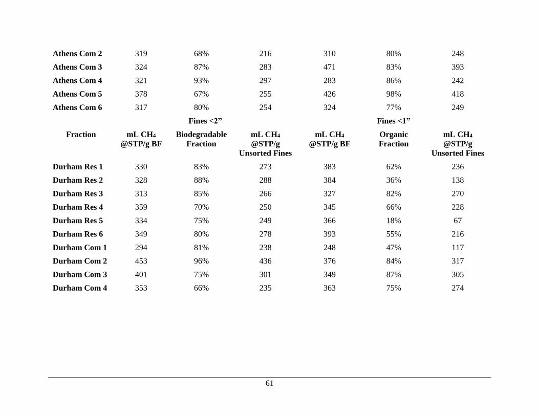
61
Athens Com 2 319 68% 216 310 80% 248
Athens Com 3 324 87% 283 471 83% 393
Athens Com 4 321 93% 297 283 86% 242
Athens Com 5 378 67% 255 426 98% 418
Athens Com 6 317 80% 254 324 77% 249
Fines <2” Fines <1”
Fraction mL CH4
@STP/g BF
Biodegradable
Fraction
mL CH4
@STP/g
Unsorted Fines
mL CH4
@STP/g BF
Organic
Fraction
mL CH4
@STP/g
Unsorted Fines
Durham Res 1 330 83% 273 383 62% 236
Durham Res 2 328 88% 288 384 36% 138
Durham Res 3 313 85% 266 327 82% 270
Durham Res 4 359 70% 250 345 66% 228
Durham Res 5 334 75% 249 366 18% 67
Durham Res 6 349 80% 278 393 55% 216
Durham Com 1 294 81% 238 248 47% 117
Durham Com 2 453 96% 436 376 84% 317
Durham Com 3 401 75% 301 349 87% 305
Durham Com 4 353 66% 235 363 75% 274

62
Appendix D. Distributions of Methane Yields by MSW Component
Figure A-0-1. Yield Frequencies of Cardboard Samples
Figure A-0-2. Yield Frequencies of Newspaper Samples
0
2
4
6
8
10
12
165 180 195 210 225 240 255 270 285 300 315 330
Fre
qu
en
cy
mL CH4 @STP/g VS
0
1
2
3
4
5
6
7
30 45 60 75 90 105 120 135 150 165 180 195 210 225 240 255 270 285 300 315 330 345
Fre
qu
en
cy
mL CH4 @STP/g VS
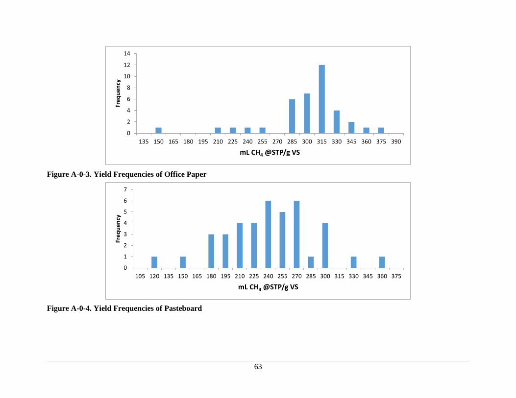
63
Figure A-0-3. Yield Frequencies of Office Paper
Figure A-0-4. Yield Frequencies of Pasteboard
0
2
4
6
8
10
12
14
135 150 165 180 195 210 225 240 255 270 285 300 315 330 345 360 375 390
Fre
qu
en
cy
mL CH4 @STP/g VS
0
1
2
3
4
5
6
7
105 120 135 150 165 180 195 210 225 240 255 270 285 300 315 330 345 360 375
Fre
qu
en
cy
mL CH4 @STP/g VS

64
Figure A-0-5. Yield Frequencies of Junk Mail
Figure A-0-6. Yield Frequencies of Aseptic Paper
0
1
2
3
4
5
6
7
8
135 150 165 180 195 210 225 240 255 270 285 300 315 330 345 360 375 390
Fre
qu
en
cy
mL CH4 @STP/g VS
0
2
4
6
8
10
120 135 150 165 180 195 210 225 240 255 270 285 300 315 330 345 360 375 390
Fre
qu
en
cy
mL CH4 @STP/g VS

65
Figure A-0-7. Yield Frequencies of Miscellaneous Paper
Figure A-0-8. Yield Frequencies of Food and Soiled Paper
0
1
2
3
4
5
6
7
8
9
105 120 135 150 165 180 195 210 225 240 255 270 285 300 315 330 345 360 375 390
Fre
qu
en
cy
mL CH4 @STP/g VS
0
1
2
3
4
5
6
60 90 120 150 180 210 240 270 300 330 360 390 420 450 480 510 540
Fre
qu
en
cy
mL CH4 @STP/g VS

66
Figure A-0-9. Yield Frequencies of Yard Waste
Figure A-0-10. Yield Frequencies of the Biodegradable Fraction of Fines <2” After Removal of Non-biodegradable Materials
0
0.5
1
1.5
2
2.5
3
3.5
4
4.5
30 45 60 75 90 105 120 135 150 165 180 195 210 225 240 255 270 285 300 315 330 345 360 375
Fre
qu
en
cy
mL CH4 @STP/g VS
0
2
4
6
8
10
12
60
75
90
10
5
12
0
13
5
15
0
16
5
18
0
19
5
21
0
22
5
24
0
25
5
27
0
28
5
30
0
31
5
33
0
34
5
36
0
37
5
39
0
40
5
42
0
43
5
45
0
46
5
48
0
Fre
qu
en
cy
mL CH4 @STP/g VS

67
Figure A-0-11. Yield Frequencies of Biodegradable Fraction of Fines <1” After Removal of Non-biodegradable Materials
Figure A-0-12. Yield Frequencies of Textiles
0
0.5
1
1.5
2
2.5
3
3.5
4
4.5
135150165180195210225240255270285300315330345360375390405420435450465480495
Fre
qu
en
cy
mL CH4 @STP/g VS
0
0.5
1
1.5
2
2.5
3
3.5
0
15
30
45
60
75
90
10
5
12
0
13
5
15
0
16
5
18
0
19
5
21
0
22
5
24
0
25
5
27
0
28
5
30
0
31
5
33
0
34
5
36
0
37
5
39
0
Fre
qu
en
cy
mL CH4 @STP/g VS

68
Figure A-0-13. Yield Frequencies of Wood
Figure A-0-14. Yield Frequencies of Composite Wood
0
1
2
3
4
5
6
7
8
0 15 30 45 60 75 90 105 120 135 150 165 180 195
Fre
qu
en
cy
mL CH4 @STP/g VS
0
1
2
3
4
5
6
7
8
0 15 30 45 60 75 90 105 120 135 150 165 180 195
Fre
qu
en
cy
mL CH4 @STP/g VS

69
Figure A-0-15. Yield Frequencies of Cellulose Controls
Figure A-0-16. Yield Frequencies of Blank Controls
0
2
4
6
8
10
12
14
270 285 300 315 330 345 360 375 390 405
Fre
qu
en
cy
mL CH4 @STP/g VS
0
5
10
15
20
25
30
35
40
45
Fre
qu
en
cy
mL CH4 @STP/(no VS added)

70
Appendix E. Waste Composition and L0 of Representative Samples
Figure A-0-17. Waste Composition and L0 of LEE988-JAN22
Category Subcategory
Mass
Percent
Moisture
Content
Volatile
SolidsEst. L0
(M3/Mg)
Normalized
L0
Cardboard 10% 27% 93% 255 17.7
Newspaper 2% 10% 98% 79 1.7
Office Paper 0% 21% 82% 369 0.4
Junk Mail 0% 13% 69% 307 0.6
Pasteboard 2% 26% 81% 200 2.8
Misc. Paper 2% 34% 81% 219 2.1
Aeseptic Cartons 1% 35% 97% 299 2.0
Food & Soiled Paper 21% 43% 91% 387 42
Yard Trash 0% 0% 0% 0 0.0
Diapers 0% 0% 0% 0 0.0
<2" Fines 16% 58% 71% 336 15.9
<1" Fines 7% 61% 76% 336 7.4
Textiles 5% 43% 87% 212 4.9
Leather 0% 0% 0% 0 0.0 LEE988-JAN22
WOOD Wood 4% 2% 96% 49 1.8 Total Sample Weight (lbs) 290
PLASTICS All Plastics 21% 2% Organic Fraction 68%
GLASS All Glass 3% 2% Inorganic Fraction 32%
METALS All Metals 3% 2% Calculated L0 (m3/Mg) 99
OTHER Inorganic Materials 1% 0% 0% 0 0.0
10:12 AM
PAPER
ORGANICS
FINES
TEXTILES
Time
Waste Composition of Lee County Truck 988
Total Load Weight (lbs) 24340
Date 01/22/14
Sample ID LEE988-JAN22
Waste Type Commercial
Truck Number 988
Cardboard , 10%
Newspaper, 2%
Office Paper, 0%
Junk Mail, 0%
Pasteboard, 2%
Misc. Paper, 2%
Aeseptic Cartons, 1%
Food & Soiled Paper, 21%
Yard Trash, 0%
Diapers, 0%
<2" Fines, 16%
<1" Fines, 7%
Textiles, 5%
Leather, 0%
Wood, 4%
All Plastics, 21%
All Glass, 3%
All Metals, 3%Inorganic
Materials, 1%

71
Figure A-0-18. Waste Composition and L0 of LEE882-JAN22
Category Subcategory
Mass
Percent
Moisture
Content
Volatile
SolidsEst. L0
(M3/Mg)
Normalized
L0
Cardboard 5% 49% 87% 169 3.9
Newspaper 1% 35% 92% 82 0.3
Office Paper 7% 30% 83% 317 12.9
Junk Mail 1% 6% 53% 328 2.1
Pasteboard 4% 41% 87% 263 5.3
Misc. Paper 5% 15% 78% 303 9.7
Aeseptic Cartons 2% 32% 83% 286 3.1
Food & Soiled Paper 24% 56% 88% 304 28
Yard Trash 0% 66% 70% 0 0.0
Diapers 2% 0% 0% 0 0.0
<2" Fines 16% 58% 78% 331 17.2
<1" Fines 5% 54% 70% 340 5.2
Textiles 1% 19% 99% 212 1.4
Leather 0% 0% 0% 0 0.0 LEEFM882-JAN22
WOOD Wood 1% 14% 89% 46 0.3 Total Sample Weight (lbs) 313
PLASTICS All Plastics 20% 2% Organic Fraction 72%
GLASS All Glass 2% 2% Inorganic Fraction 28%
METALS All Metals 5% 2% Calculated L0 (m3/Mg) 89
OTHER Inorganic Materials 0% 0% 0% 0 0.0
PAPER
ORGANICS
FINES
TEXTILES
Total Load Weight (lbs) 22580
Date 01/22/14
Time 8:02 AM
Truck Number FM882
Waste Composition of Lee County Truck FM882
Sample ID LEEFM882-JAN22
Waste Type CommercialCardboard , 5%
Newspaper, 1%
Office Paper, 7%
Junk Mail, 1%
Pasteboard, 4%
Misc. Paper, 5%Aeseptic
Cartons, 2%
Food & Soiled Paper, 24%
Yard Trash, 0%
Diapers, 2%
<2" Fines, 16%
<1" Fines, 5%
Textiles, 1%
Leather, 0%
Wood, 1% All Plastics, 20%
All Glass, 2%
All Metals, 5%Inorganic
Materials, 0%
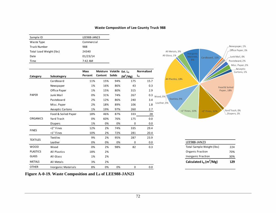
72
Figure A-0-19. Waste Composition and L0 of LEE988-JAN23
Category Subcategory
Mass
Percent
Moisture
Content
Volatile
SolidsEst. L0
(M3/Mg)
Normalized
L0
Cardboard 11% 15% 94% 175 15.7
Newspaper 1% 16% 86% 43 0.3
Office Paper 1% 15% 80% 315 2.9
Junk Mail 0% 31% 74% 267 0.3
Pasteboard 2% 12% 86% 240 3.4
Misc. Paper 2% 18% 89% 106 1.8
Aeseptic Cartons 1% 19% 97% 260 2.7
Food & Soiled Paper 18% 46% 87% 333 28
Yard Trash 0% 60% 76% 175 0.0
Diapers 1% 0% 0% 0 0.0
<2" Fines 12% 2% 74% 335 29.4
<1" Fines 10% 2% 72% 281 20.4
Textiles 9% 2% 95% 287 23.9
Leather 0% 0% 0% 0 0.0 LEE988-JAN23
WOOD Wood 0% 2% 98% 82 0.3 Total Sample Weight (lbs) 224
PLASTICS All Plastics 18% 2% Organic Fraction 70%
GLASS All Glass 1% 2% Inorganic Fraction 30%
METALS All Metals 3% 2% Calculated L0 (m3/Mg) 129
OTHER Inorganic Materials 8% 0% 0% 0 0.0
PAPER
ORGANICS
FINES
TEXTILES
Total Load Weight (lbs) 24340
Date 01/23/14
Time 7:42 AM
Truck Number 988
Waste Composition of Lee County Truck 988
Sample ID LEE988-JAN23
Waste Type Commercial
Cardboard , 11%
Newspaper, 1%
Office Paper, 1%
Junk Mail, 0%
Pasteboard, 2%
Misc. Paper, 2%
Aeseptic Cartons, 1%
Food & Soiled Paper, 18%
Yard Trash, 0%Diapers, 1%
<2" Fines, 12%<1" Fines, 10%
Textiles, 9%
Leather, 0%
Wood, 0%
All Plastics, 18%
All Glass, 1%
All Metals, 3%Inorganic Materials,
8%
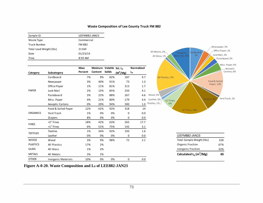
73
Figure A-0-20. Waste Composition and L0 of LEE882-JAN23
Category Subcategory
Mass
Percent
Moisture
Content
Volatile
SolidsEst. L0
(M3/Mg)
Normalized
L0
Cardboard 7% 9% 82% 187 9.7
Newspaper 3% 40% 91% 73 1.3
Office Paper 1% 11% 81% 313 1.7
Junk Mail 2% 15% 85% 250 4.1
Pasteboard 3% 22% 88% 267 4.6
Misc. Paper 4% 21% 80% 179 4.4
Aeseptic Cartons 0% 20% 94% 300 1.0
Food & Soiled Paper 12% 62% 92% 318 14
Yard Trash 1% 0% 0% 0 0.0
Diapers 8% 0% 0% 0 0.0
<2" Fines 18% 42% 63% 265 17.7
<1" Fines 6% 51% 75% 142 3.1
Textiles 1% 34% 92% 193 1.6
Leather 0% 0% 0% 0 0.0 LEEFM882-JAN23
WOOD Wood 3% 9% 98% 72 2.1 Total Sample Weight (lbs) 328
PLASTICS All Plastics 17% 2% Organic Fraction 67%
GLASS All Glass 1% 2% Inorganic Fraction 33%
METALS All Metals 3% 2% Calculated L0 (m3/Mg) 65
OTHER Inorganic Materials 10% 0% 0% 0 0.0
PAPER
ORGANICS
FINES
TEXTILES
Total Load Weight (lbs) 21160
Date 01/23/14
Time 8:59 AM
Truck Number FM 882
Waste Composition of Lee County Truck FM 882
Sample ID LEEFM882-JAN23
Waste Type Commercial
Cardboard , 7%
Newspaper, 3%
Office Paper, 1%
Junk Mail, 2%
Pasteboard, 3%
Misc. Paper, 4%
Aeseptic Cartons, 0%
Food & Soiled Paper, 12%
Yard Trash, 1%Diapers, 8%
<2" Fines, 18%
<1" Fines, 6%Textiles, 1%
Leather, 0%
Wood, 3%
All Plastics, 17%
All Glass, 1%
All Metals, 3% Inorganic Materials, 10%
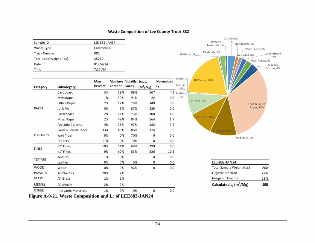
74
Figure A-0-21. Waste Composition and L0 of LEE882-JAN24
Category Subcategory
Mass
Percent
Moisture
Content
Volatile
SolidsEst. L0
(M3/Mg)
Normalized
L0
Cardboard 3% 19% 89% 167 4.1
Newspaper 1% 39% 91% 22 0.2
Office Paper 2% 12% 79% 349 3.8
Junk Mail 0% 9% 87% 285 0.0
Pasteboard 2% 11% 73% 300 4.0
Misc. Paper 2% 49% 84% 164 1.7
Aeseptic Cartons 4% 26% 97% 282 7.2
Food & Soiled Paper 33% 45% 86% 374 59
Yard Trash 0% 0% 70% 0 0.0
Diapers 11% 0% 0% 0 0.0
<2" Fines 10% 54% 69% 299 9.6
<1" Fines 9% 60% 83% 336 10.2
Textiles 1% 0% 0 0.0
Leather 0% 0% 0% 0 0.0 LEE-882-JAN24
WOOD Wood 0% 0% 92% 0 0.0 Total Sample Weight (lbs) 260
PLASTICS All Plastics 20% 2% Organic Fraction 77%
GLASS All Glass 1% 2% Inorganic Fraction 23%
METALS All Metals 2% 2% Calculated L0 (m3/Mg) 100
OTHER Inorganic Materials 1% 0% 0% 0 0.0
PAPER
ORGANICS
FINES
TEXTILES
Total Load Weight (lbs) 25260
Date 01/24/14
Time 7:27 AM
Truck Number 882
Waste Composition of Lee County Truck 882
Sample ID LEE-882-JAN24
Waste Type Commercial
Cardboard , 3%
Newspaper, 1%
Office Paper, 2%
Junk Mail, 0%Pasteboard,
2%Misc. Paper, 2%
Aeseptic Cartons, 4%
Food & Soiled Paper, 33%
Yard Trash, 0%
Diapers, 11%
<2" Fines, 10%
<1" Fines, 9%
Textiles, 1%
Leather, 0%
Wood, 0%All Plastics, 20%
All Glass, 1%All Metals, 2%
Inorganic Materials, 1%

75
Figure A-0-22. Waste Composition and L0 of LEE988-JAN24
Category Subcategory
Mass
Percent
Moisture
Content
Volatile
SolidsEst. L0
(M3/Mg)
Normalized
L0
Cardboard 5% 9% 91% 166 6.6
Newspaper 0% 0% 0% 0 0.0
Office Paper 6% 7% 80% 229 10.8
Junk Mail 0% 13% 86% 318 0.9
Pasteboard 2% 14% 86% 261 4.7
Misc. Paper 6% 11% 74% 303 12.8
Aeseptic Cartons 1% 17% 99% 272 1.3
Food & Soiled Paper 8% 48% 94% 293 11
Yard Trash 0% 44% 85% 97 0.0
Diapers 0% 0% 0% 0 0.0
<2" Fines 4% 54% 92% 256 3.9
<1" Fines 4% 67% 84% 168 1.8
Textiles 5% 7% 94% 143 5.8
Leather 0% 0% 0% 0 0.0 LEE988-JAN24
WOOD Wood 0% 9% 91% 36 0.1 Total Sample Weight (lbs) 212
PLASTICS All Plastics 17% 2% Organic Fraction 49%
GLASS All Glass 0% 2% Inorganic Fraction 51%
METALS All Metals 6% 2% Calculated L0 (m3/Mg) 60
OTHER Inorganic Materials 19% 0% 0% 0 0.0
PAPER
ORGANICS
FINES
TEXTILES
Total Load Weight (lbs) 29500
Date 01/24/14
Time 7:24 AM
Truck Number 988
Waste Composition of Lee County Truck 988
Sample ID LEE988-JAN24
Waste Type CommercialCardboard , 5%
Newspaper, 0%
Office Paper, 6%
Junk Mail, 0%
Pasteboard, 2%
Misc. Paper, 6%Aeseptic
Cartons, 1%
Food & Soiled Paper, 8%
Yard Trash, 0%
Diapers, 0%
<2" Fines, 4%
<1" Fines, 4%
Textiles, 5%
Leather, 0%
Wood, 0%
All Plastics, 17%
All Glass, 0%
All Metals, 6%
Inorganic Materials, 19%

76
Figure A-0-23. Waste Composition and L0 of LEE61108-JAN22
Category Subcategory
Mass
Percent
Moisture
Content
Volatile
SolidsEst. L0
(M3/Mg)
Normalized
L0
Cardboard 0% 0% 0% 0 0.0
Newspaper 0% 10% 94% 84 0.3
Office Paper 0% 9% 84% 287 0.8
Junk Mail 0% 12% 69% 0 0.0
Pasteboard 3% 22% 86% 175 3.8
Misc. Paper 9% 12% 69% 132 7.4
Aeseptic Cartons 0% 19% 91% 0 0.0
Food & Soiled Paper 25% 51% 82% 322 32
Yard Trash 0% 0% 0% 0 0.0
Diapers 7% 0% 0% 0 0.0
<2" Fines 15% 61% 72% 232 9.5
<1" Fines 3% 59% 60% 154 1.3
Textiles 6% 1% 99% 20 1.1
Leather 0% 2% 0.0 LEEC61108-JAN22
WOOD Wood 2% 7% 80% 0 0.0 Total Sample Weight (lbs) 267
PLASTICS All Plastics 17% 2% Organic Fraction 70%
GLASS All Glass 5% 2% Inorganic Fraction 30%
METALS All Metals 4% 2% Calculated L0 (m3/Mg) 56
OTHER Inorganic Materials 1% 0% 0% 0 0.0
PAPER
ORGANICS
FINES
TEXTILES
Total Load Weight (lbs) 14940
Date 01/22/14
Time 10:16 AM
Truck Number C61108
Waste Composition of Lee County Truck C61108
Sample ID LEEC61108-JAN22
Waste Type ResidentialCardboard ,
0%
Newspaper, 0%Office Paper, 0%
Junk Mail, 0%
Pasteboard, 3%
Misc. Paper, 9%
Aeseptic Cartons, 0%
Food & Soiled Paper, 25%
Yard Trash, 0%Diapers, 7%
<2" Fines, 15%<1" Fines, 3%
Textiles, 6%
Leather, 0%
Wood, 2%
All Plastics, 17%
All Glass, 5%
All Metals, 4%
Inorganic Materials,
1%

77
Figure A-0-24. Waste Composition and L0 of LEE4023-JAN22
Category Subcategory
Mass
Percent
Moisture
Content
Volatile
SolidsEst. L0
(M3/Mg)
Normalized
L0
Cardboard 2% 14% 84% 224 3.9
Newspaper 1% 24% 84% 184 0.8
Office Paper 0% 11% 84% 294 0.4
Junk Mail 0% 20% 69% 0 0.0
Pasteboard 0% 25% 83% 246 0.7
Misc. Paper 6% 20% 69% 209 6.9
Aeseptic Cartons 0% 19% 91% 208 0.6
Food & Soiled Paper 9% 69% 91% 272 7
Yard Trash 30% 29% 83% 134 23.7
Diapers 3% 0% 0% 0 0.0
<2" Fines 11% 57% 79% 163 5.8
<1" Fines 6% 45% 55% 159 2.8
Textiles 6% 10% 85% 3 0.1
Leather 0% 0% 0% 0 0.0 LEEV4023-JAN22
WOOD Wood 2% 15% 83% 44 0.7 Total Sample Weight (lbs) 252
PLASTICS All Plastics 15% 2% Organic Fraction 75%
GLASS All Glass 2% 2% Inorganic Fraction 25%
METALS All Metals 5% 2% Calculated L0 (m3/Mg) 54
OTHER Inorganic Materials 1% 0% 0% 0 0.0
PAPER
ORGANICS
FINES
TEXTILES
Total Load Weight (lbs) 6580
Date 01/22/14
Time 10:26 AM
Truck Number V4023
Waste Composition of Lee County Truck V4023
Sample ID LEEV4023-JAN22
Waste Type Residential
Cardboard , 2%
Newspaper, 1%
Office Paper, 0%
Junk Mail, 0%
Pasteboard, 0%
Misc. Paper, 6%
Aeseptic Cartons, 0%
Food & Soiled Paper, 9%
Yard Trash, 30%
Diapers, 3%
<2" Fines, 11%
<1" Fines, 6%
Textiles, 6%
Leather, 0%
Wood, 2%
All Plastics, 15%
All Glass, 2%
All Metals, 5%
Inorganic Materials, 1%

78
Figure A-0-25. Waste Composition and L0 of LEE406-JAN22
Category Subcategory
Mass
Percent
Moisture
Content
Volatile
SolidsEst. L0
(M3/Mg)
Normalized
L0
Cardboard 3% 24% 81% 217 4.2
Newspaper 1% 16% 83% 149 0.7
Office Paper 0% 14% 82% 289 0.4
Junk Mail 0% 8% 74% 311 0.4
Pasteboard 2% 23% 88% 246 2.8
Misc. Paper 7% 17% 76% 290 12.2
Aeseptic Cartons 0% 33% 89% 252 0.5
Food & Soiled Paper 8% 52% 88% 294 10
Yard Trash 0% 53% 34% 61 0.0
Diapers 6% 0% 0% 0 0.0
<2" Fines 15% 55% 75% 34 1.7
<1" Fines 9% 42% 49% 118 3.1
Textiles 4% 8% 98% 299 10.8
Leather 0% 0% 0% 0 0.0 LEEP406-JAN22
WOOD Wood 6% 18% 91% 26 1.1 Total Sample Weight (lbs) 276
PLASTICS All Plastics 19% 2% Organic Fraction 59%
GLASS All Glass 1% 2% Inorganic Fraction 41%
METALS All Metals 8% 2% Calculated L0 (m3/Mg) 48
OTHER Inorganic Materials 11% 0% 0% 0 0.0
PAPER
ORGANICS
FINES
TEXTILES
Total Load Weight (lbs) 26040
Date 01/22/14
Time 4:00 PM
Truck Number P406
Waste Composition of Lee County Truck P406
Sample ID LEEP406-JAN22
Waste Type Residential Cardboard , 3%
Newspaper, 1%Office Paper, 0%
Junk Mail, 0%
Pasteboard, 2%
Misc. Paper, 7%
Aeseptic Cartons, 0%
Food & Soiled Paper, 8% Yard
Trash, 0%
Diapers, 6%
<2" Fines, 15%
<1" Fines, 9%
Textiles, 4%
Leather, 0%
Wood, 6%
All Plastics, 19%
All Glass, 1%
All Metals, 8%
Inorganic Materials, 11%

79
Figure A-0-26. Waste Composition and L0 of LEE4023-JAN23
Category Subcategory
Mass
Percent
Moisture
Content
Volatile
SolidsEst. L0
(M3/Mg)
Normalized
L0
Cardboard 7% 15% 84% 235 11.8
Newspaper 1% 16% 93% 111 0.9
Office Paper 2% 7% 85% 338 4.2
Junk Mail 2% 10% 77% 319 3.5
Pasteboard 1% 16% 89% 269 1.8
Misc. Paper 3% 7% 67% 279 4.8
Aeseptic Cartons 0% 14% 95% 264 0.8
Food & Soiled Paper 11% 51% 88% 375 18
Yard Trash 26% 38% 89% 105 15.2
Diapers 6% 0% 0% 0 0.0
<2" Fines 6% 48% 78% 190 4.7
<1" Fines 2% 45% 77% 162 1.3
Textiles 5% 25% 90% 207 6.9
Leather 0% 0% 0% 0 0.0 LEE4023-JAN23
WOOD Wood 9% 11% 86% 16 1.1 Total Sample Weight (lbs) 407
PLASTICS All Plastics 6% 2% Organic Fraction 79%
GLASS All Glass 2% 2% Inorganic Fraction 21%
METALS All Metals 6% 2% Calculated L0 (m3/Mg) 75
OTHER Inorganic Materials 6% 0% 0% 0 0.0
PAPER
ORGANICS
FINES
TEXTILES
Total Load Weight (lbs) 24340
Date 01/23/14
Time 11:40 AM
Truck Number 4023
Waste Composition of Lee County Truck 4023
Sample ID LEE4023-JAN23
Waste Type Residential
Cardboard , 7%
Newspaper, 1%
Office Paper, 2%
Junk Mail, 2%
Pasteboard, 1%
Misc. Paper, 3%
Aeseptic Cartons, 0%
Food & Soiled Paper, 11%
Yard Trash, 26%
Diapers, 6%
<2" Fines, 6%
<1" Fines, 2%
Textiles, 5%Leather,
0%
Wood, 9%
All Plastics, 6%
All Glass, 2%All
Metals, 6%
Inorganic Materials, 6%

80
Figure A-0-27. Waste Composition and L0 of LEE4001-JAN23
Category Subcategory
Mass
Percent
Moisture
Content
Volatile
SolidsEst. L0
(M3/Mg)
Normalized
L0
Cardboard 0% 10% 87% 249 0.5
Newspaper 2% 25% 89% 126 1.9
Office Paper 0% 0% 0% 0 0.0
Junk Mail 0% 36% 79% 0 0.0
Pasteboard 2% 31% 90% 242 2.9
Misc. Paper 2% 20% 78% 273 2.9
Aeseptic Cartons 0% 21% 92% 248 0.3
Food & Soiled Paper 22% 38% 74% 333 35
Yard Trash 0% 0% 0% 0 0.0
Diapers 5% 0% 0% 0 0.0
<2" Fines 12% 53% 73% 127 5.1
<1" Fines 5% 54% 59% 226 3.2
Textiles 0% 22% 91% 177 0.3
Leather 0% 0% 0% 0 0.0 LEE4001-JAN23
WOOD Wood 12% 13% 94% 0 0.0 Total Sample Weight (lbs) 273
PLASTICS All Plastics 14% 2% Organic Fraction 62%
GLASS All Glass 2% 2% Inorganic Fraction 38%
METALS All Metals 5% 2% Calculated L0 (m3/Mg) 52
OTHER Inorganic Materials 16% 0% 0% 0 0.0
PAPER
ORGANICS
FINES
TEXTILES
Total Load Weight (lbs) 16460
Date 01/23/14
Time 12:01 PM
Truck Number 4001
Waste Composition of Lee County Truck 4001
Sample ID LEE4001-JAN23
Waste Type Residential
Cardboard , 0%
Newspaper, 2%
Office Paper, 0% Junk Mail, 0%
Pasteboard, 2%
Misc. Paper, 2%
Aeseptic Cartons, 0%
Food & Soiled Paper, 22%
Yard Trash, 0%Diapers, 5%
<2" Fines, 12%
<1" Fines, 5%
Textiles, 0%
Leather, 0%
Wood, 12%
All Plastics, 14%
All Glass, 2%
All Metals,
5%
Inorganic Materials, 16%

81
Figure A-0-28. Waste Composition and L0 of LEE388-JAN23
Category Subcategory
Mass
Percent
Moisture
Content
Volatile
SolidsEst. L0
(M3/Mg)
Normalized
L0
Cardboard 1% 32% 81% 170 1.3
Newspaper 1% 15% 92% 92 0.9
Office Paper 0% 10% 78% 335 0.0
Junk Mail 1% 7% 75% 310 2.4
Pasteboard 2% 14% 79% 232 3.4
Misc. Paper 5% 14% 83% 222 7.2
Aeseptic Cartons 1% 18% 96% 262 1.8
Food & Soiled Paper 22% 54% 89% 347 31
Yard Trash 0% 34% 76% 72 0.0
Diapers 11% 0% 0% 0 0.0
<2" Fines 16% 52% 76% 121 7.0
<1" Fines 4% 50% 68% 196 2.7
Textiles 3% 16% 98% 207 5.4
Leather 0% 0% 0% 0 0.0 LEEP388-JAN23
WOOD Wood 5% 28% 89% 34 1.0 Total Sample Weight (lbs) 353
PLASTICS All Plastics 14% 2% Organic Fraction 71%
GLASS All Glass 2% 2% Inorganic Fraction 29%
METALS All Metals 5% 2% Calculated L0 (m3/Mg) 64
OTHER Inorganic Materials 6% 0% 0% 0 0.0
PAPER
ORGANICS
FINES
TEXTILES
Total Load Weight (lbs) 26180
Date 01/23/14
Time 2:56 PM
Truck Number P388
Waste Composition of Lee County Truck P388
Sample ID LEEP388-JAN23
Waste Type Residential Cardboard , 1%
Newspaper, 1%
Office Paper, 0%
Junk Mail, 1% Pasteboard, 2%
Misc. Paper, 5%
Aeseptic Cartons, 1%
Food & Soiled Paper, 22%
Yard Trash, 0%Diapers, 11%
<2" Fines, 16%<1" Fines, 4%
Textiles, 3%
Leather, 0%
Wood, 5%
All Plastics, 14%
All Glass, 2% All Metals
, 5%
Inorganic Materials,
6%

82
Figure A-0-29. Waste Composition and L0 of UF Transfer Station Com-1
Category Subcategory
Mass
Percent
Moisture
Content
Volatile
SolidsEst. L0
(M3/Mg)
Normalized
L0
Cardboard 6% 18% 92% 227 9.8
Newspaper 2% 33% 87% 55 0.7
Office Paper 6% 22% 75% 275 8.9
Junk Mail 2% 19% 76% 240 3.0
Pasteboard 4% 16% 90% 297 9.2
Misc. Paper 1% 18% 86% 213 1.5
Aeseptic Cartons 2% 21% 93% 232 2.9
Food & Soiled Paper 30% 47% 96% 257 38.6
Yard Trash 1% 24% 88% 172 1.4
<2" Fines 9% 55% 77% 173 5.3
<1" Fines 4% 38% 50% 188 2.3
TEXTILES Organic Textiles 2% 2% 98% 212 4.1
Leather 0% 0% 0% 0 0.0
WOOD Wood 0% 0% 0% 0 0.0 UF COM 1
PLASTICS All Plastics 21% Total Sample Weight (lbs) 219
GLASS All Glass 1% Organic Fraction 73%
METALS All Metals 4% Inorganic Fraction 27%
OTHER Inorganic Materials 0% Calculated L0 (m3/Mg) 88
Human & Animal Waste 5% 0% 0% 0 0.0
PAPER
ORGANICS
FINES
Total Load Weight (lbs)
Date 04/23/14
Time 10:12 AM
Truck Number 3510
Waste Composition of UF Waste Truck 3510
Sample ID UF COM 1
Waste Type Commercial Cardboard , 6%
Newspaper, 2%
Office Paper, 6% Junk Mail, 2%
Pasteboard, 4%
Misc. Paper, 1%
Aeseptic
Cartons, 2%
Food & Soiled Paper, 30%
Yard Trash, 1%<2" Fines, 9%
<1" Fines, 4%
Organic Textiles, 2%
All Plastics, 21%
All Glass, 1%
All Metals, 4%
Inorganic Materials, 0%

83
Figure A-0-30. Waste Composition and L0 of UF Transfer Station Com-2
Category Subcategory
Mass
Percent
Moisture
Content
Volatile
SolidsEst. L0
(M3/Mg)
Normalized
L0
Cardboard 5% 25% 81% 225 7.1
Newspaper 5% 14% 84% 83 2.9
Office Paper 5% 0% 0% 275 0.0
Junk Mail 1% 14% 82% 298 2.6
Pasteboard 1% 8% 82% 226 2.1
Misc. Paper 2% 9% 82% 324 5.1
Aeseptic Cartons 2% 26% 99% 286 4.8
Food & Soiled Paper 26% 72% 97% 262 18.8
Yard Trash 1% 24% 88% 172 1.0
<2" Fines 12% 48% 93% 176 9.7
<1" Fines 2% 48% 72% 187 1.6
TEXTILES Organic Textiles 1% 2% 98% 212 2.6
Leather 0% 0% 0% 0 0.0
WOOD Wood 0% 0% 0% 0 0.0 UF COM 2
PLASTICS All Plastics 27% Total Sample Weight (lbs) 330
GLASS All Glass 1% Organic Fraction 65%
METALS All Metals 6% Inorganic Fraction 35%
OTHER Inorganic Materials 2% Calculated L0 (m3/Mg) 58
Human & Animal Waste 1% 0% 0% 0 0.0
PAPER
ORGANICS
FINES
Total Load Weight (lbs)
Date 04/23/14
Time 12:00 AM
Truck Number 4538
Waste Composition of UF Waste Truck 4538
Sample ID UF COM 2
Waste Type Commercial
Cardboard , 5%
Newspaper, 5%
Office Paper, 5%
Junk Mail, 1%
Pasteboard, 1%
Misc. Paper, 2%
Aeseptic Cartons, 2%
Food & Soiled Paper, 26%
Yard Trash, 1%
<2" Fines, 12%
<1" Fines, 2%
Organic Textiles, 1%
Leather, 0%
Wood, 0%
All Plastics, 27%
All Glass, 1%
All Metals,
6%
Inorganic Materials, 2%

84
Figure A-0-31. Waste Composition and L0 of UF Transfer Station Com-3
Category Subcategory
Mass
Percent
Moisture
Content
Volatile
SolidsEst. L0
(M3/Mg)
Normalized
L0
Cardboard 5% 13% 82% 280 11.0
Newspaper 1% 53% 98% 78 0.3
Office Paper 3% 35% 76% 304 5.2
Junk Mail 1% 7% 69% 224 0.8
Pasteboard 1% 11% 74% 221 1.5
Misc. Paper 2% 0% 0% 213 0.0
Aeseptic Cartons 3% 26% 98% 255 5.9
Food & Soiled Paper 26% 36% 100% 271 45.0
Yard Trash 0% 0% 0% 0 0.0
<2" Fines 6% 51% 89% 182 5.2
<1" Fines 2% 49% 73% 101 0.7
TEXTILES Organic Textiles 0% 0% 0% 0 0.0
Leather 0% 0% 0% 0 0.0
WOOD Wood 8% 0% 0% 0 0.0 UF COM 3
PLASTICS All Plastics 21% Total Sample Weight (lbs) 330
GLASS All Glass 1% Organic Fraction 61%
METALS All Metals 3% Inorganic Fraction 39%
OTHER Inorganic Materials 14% Calculated L0 (m3/Mg) 76
Human & Animal Waste 2% 0% 0% 0 0.0
PAPER
ORGANICS
FINES
Total Load Weight (lbs)
Date 04/23/14
Time 11:10 AM
Truck Number 4538
Waste Composition of UF Waste Truck 4538
Sample ID UF COM 3
Waste Type Commercial
Cardboard , 5%
Newspaper, 1%Office Paper, 3%
Junk Mail, 1%
Pasteboard, 1%
Misc. Paper, 2%
Aeseptic Cartons, 3%
Food & Soiled Paper, 26%
Yard Trash, 0%
<2" Fines, 6%
<1" Fines, 2%Organic
Textiles, 0%
Leather, 0%
Wood, 8%
All Plastics, 21%
All Glass, 1%
All Metals, 3%
Inorganic Materials, 14%

85
Figure A-0-32. Waste Composition and L0 of UF Transfer Station Com-4
Category Subcategory
Mass
Percent
Moisture
Content
Volatile
SolidsEst. L0
(M3/Mg)
Normalized
L0
Cardboard 3% 17% 84% 194 4.2
Newspaper 0% 25% 92% 116 0.4
Office Paper 2% 14% 75% 289 3.6
Junk Mail 1% 18% 71% 218 1.7
Pasteboard 2% 25% 82% 252 3.8
Misc. Paper 3% 37% 73% 274 3.2
Aeseptic Cartons 1% 26% 98% 260 2.7
Food & Soiled Paper 23% 64% 94% 258 20.0
Yard Trash 1% 63% 90% 115 0.3
<2" Fines 11% 51% 93% 146 7.5
<1" Fines 3% 39% 31% 106 0.6
TEXTILES Organic Textiles 9% 2% 98% 212 17.5
Leather 0% 0% 0% 0 0.0
WOOD Wood 0% 0% 0% 0 0.0 UF COM 4
PLASTICS All Plastics 28% Total Sample Weight (lbs)
GLASS All Glass 1% Organic Fraction 68%
METALS All Metals 2% Inorganic Fraction 32%
OTHER Inorganic Materials 0% Calculated L0 (m3/Mg) 65
Human & Animal Waste 4% 0% 0% 0 0.0
Truck Number 4538
Waste Composition of UF Waste Truck 4538
Sample ID UF COM 4
Waste Type Commercial
PAPER
ORGANICS
FINES
Total Load Weight (lbs)
Date 04/24/14
Time 11:00 AM
Cardboard , 3%
Newspaper, 0% Office Paper, 2%
Junk Mail, 1%
Pasteboard, 2%
Misc. Paper, 3%
Aeseptic Cartons, 1%
Food & Soiled Paper, 23%
Yard Trash, 1%<2" Fines, 11%
<1" Fines, 3%
Organic Textiles, 9%
Leather, 0%
Wood, 0%
All Plastics, 28%
All Glass, 1%
All Metals, 2%
Inorganic Materials, 0%

86
Figure A-0-33. Waste Composition and L0 of UF Transfer Station Com-5
Category Subcategory
Mass
Percent
Moisture
Content
Volatile
SolidsEst. L0
(M3/Mg)
Normalized
L0
Cardboard 6% 29% 90% 199 8.2
Newspaper 2% 17% 93% 38 0.6
Office Paper 9% 35% 87% 148 7.2
Junk Mail 2% 15% 74% 273 3.5
Pasteboard 3% 21% 76% 218 4.1
Misc. Paper 3% 16% 92% 219 5.4
Aeseptic Cartons 2% 27% 100% 242 3.7
Food & Soiled Paper 30% 34% 88% 347 61.8
Yard Trash 0% 0% 0% 0 0.0
<2" Fines 8% 52% 85% 182 5.8
<1" Fines 2% 48% 90% 177 1.4
TEXTILES Organic Textiles 7% 2% 98% 212 13.9
Leather 0% 0% 0% 0 0.0
WOOD Wood 0% 0% 0% 0 0.0 UF COM 5
PLASTICS All Plastics 20% Total Sample Weight (lbs)
GLASS All Glass 1% Organic Fraction 75%
METALS All Metals 3% Inorganic Fraction 25%
OTHER Inorganic Materials 1% Calculated L0 (m3/Mg) 116
Human & Animal Waste 1% 0% 0% 0 0.0
PAPER
ORGANICS
FINES
Total Load Weight (lbs)
Date 04/25/14
Time 2:22 PM
Truck Number 4538
Waste Composition of UF Waste Truck 4538
Sample ID UF COM 5
Waste Type Commercial
Cardboard , 6%
Newspaper, 2%
Office Paper, 9% Junk Mail, 2%
Pasteboard, 3%
Misc. Paper, 3%
Aeseptic Cartons, 2%
Food & Soiled Paper, 30%
Yard Trash, 0%
<2" Fines, 8%<1" Fines, 2%
Organic Textiles, 7%
Leather, 0%
Wood, 0%
All Plastics, 20%
All Glass, 1%
All Metals, 3% Inorganic Materials, 1%

87
Figure A-0-34. Waste Composition and L0 of ACC Com1
Category Subcategory
Mass
Percent
Moisture
Content
Volatile
SolidsEst. L0
(M3/Mg)
Normalized
L0
Cardboard 6% 42% 87% 234 6.8
Newspaper 1% 24% 94% 116 0.6
Office Paper 4% 18% 83% 314 8.0
Junk Mail 2% 6% 78% 283 3.6
Pasteboard 2% 21% 91% 249 4.1
Misc. Paper 4% 15% 79% 301 8.5
Aeseptic Cartons 1% 25% 95% 273 2.6
Food & Soiled Paper 24% 41% 98% 310 43.5
Yard Trash 11% 49% 78% 0 0.0
<2" Fines 10% 53% 88% 189 8.1
<1" Fines 5% 45% 80% 417 9.0
TEXTILES Organic Textiles 3% 8% 100% 266 7.4
Leather 0% 0% 0% 0 0.0
WOOD Wood 0% 0% 0% 0 0.0 ATH COM 1
PLASTICS All Plastics 17% Total Sample Weight (lbs) 268
GLASS All Glass 1% Organic Fraction 78%
METALS All Metals 2% Inorganic Fraction 22%
OTHER Inorganic Materials 2% Calculated L0 (m3/Mg) 102
Human & Animal Waste 0% 0% 0% 0 0.0
ORGANICS
FINES
PAPER
Total Load Weight (lbs) 16380
Date March 4 2015
Time 8:00 AM
Truck Number 30-40-503
Waste Composition of Athens County Truck 30-40-503
Sample ID ATH COM 1
Waste Type Commercial
Cardboard , 6%
Newspaper, 1%
Office Paper, 4%
Junk Mail, 2%
Pasteboard, 2%
Misc. Paper, 4%
Aeseptic Cartons, 1%
Food & Soiled Paper, 24%
Yard Trash, 11%
<2" Fines, 10%
<1" Fines, 5%
Organic Textiles, 3%
Leather, 0%
Wood, 0%
All Plastics, 17%
All Glass, 1%
All Metals, 2%
Inorganic Materials, 2%

88
Figure A-0-35. Waste Composition and L0 of ACC Com2
Category Subcategory
Mass
Percent
Moisture
Content
Volatile
SolidsEst. L0
(M3/Mg)
Normalized
L0
Cardboard 5% 52% 93% 232 5.5
Newspaper 1% 24% 98% 77 0.5
Office Paper 2% 12% 83% 311 3.6
Junk Mail 1% 19% 76% 333 1.2
Pasteboard 1% 20% 91% 231 2.5
Misc. Paper 3% 32% 97% 212 4.3
Aeseptic Cartons 3% 41% 93% 273 3.8
Food & Soiled Paper 22% 67% 98% 216 15.0
Yard Trash 0% 77% 91% 226 0.0
<2" Fines 1% 73% 86% 217 0.5
<1" Fines 1% 41% 76% 227 0.6
TEXTILES Organic Textiles 1% 47% 97% 324 2.4
Leather 0% 0% 0% 0 0.0
WOOD Wood 11% 12% 100% 171 16.5 ATH COM 2
PLASTICS All Plastics 24% Total Sample Weight (lbs)
GLASS All Glass 1% Organic Fraction 57%
METALS All Metals 1% Inorganic Fraction 43%
OTHER Inorganic Materials 17% Calculated L0 (m3/Mg) 57
Human & Animal Waste 4% 0% 0% 0 0.0
PAPER
ORGANICS
FINES
Total Load Weight (lbs) 30520
Date March 4 2015
Time 3:00 PM
Truck Number 30-40-503
Waste Composition of Athens County Truck 30-40-503
Sample ID ATH COM 2
Waste Type Commercial Cardboard , 5%
Newspaper, 1%
Office Paper, 2%
Junk Mail, 1%
Pasteboard, 1%
Misc. Paper, 3%
Aeseptic Cartons, 3%
Food & Soiled Paper, 22%
Yard Trash, 0%
<2" Fines, 1%
<1" Fines, 1%
Organic Textiles, 1%
Leather, 0%
Wood, 11%
All Plastics, 24%
All Glass, 1%
All Metals,
1%
Inorganic Materials, 17%

89
Figure A-0-36. Waste Composition and L0 of ACC Com3
Category Subcategory
Mass
Percent
Moisture
Content
Volatile
SolidsEst. L0
(M3/Mg)
Normalized
L0
Cardboard 5% 16% 91% 239 9.5
Newspaper 4% 16% 98% 40 1.2
Office Paper 5% 5% 81% 306 10.9
Junk Mail 1% 42% 74% 303 1.3
Pasteboard 4% 27% 87% 218 5.3
Misc. Paper 2% 23% 70% 315 4.1
Aeseptic Cartons 1% 22% 93% 244 0.9
Food & Soiled Paper 24% 31% 79% 393 50.4
Yard Trash 0% 49% 78% 124 0.2
<2" Fines 9% 65% 87% 331 9.5
<1" Fines 4% 57% 83% 356 5.4
TEXTILES Organic Textiles 0% 62% 94% 365 0.3
Leather 0% 0% 0% 0 0.0
WOOD Wood 2% 14% 84% 46 0.8 ATH COM 3
PLASTICS All Plastics 17% Total Sample Weight (lbs)
GLASS All Glass 6% Organic Fraction 69%
METALS All Metals 6% Inorganic Fraction 31%
OTHER Inorganic Materials 2% Calculated L0 (m3/Mg) 100
Human & Animal Waste 3% 0% 0% 0 0.0
PAPER
ORGANICS
FINES
Total Load Weight (lbs) 26800
Date March 6 2015
Time 7:30 AM
Truck Number 160-30-40-503
Waste Composition of Athens County Truck 160-30-40-503
Sample ID ATH COM 3
Waste Type CommercialCardboard , 5%
Newspaper, 4%
Office Paper, 5%
Junk Mail, 1%
Pasteboard, 4%
Misc. Paper, 2%
Aeseptic Cartons, 1%
Food & Soiled Paper, 24%
Yard Trash, 0%
<2" Fines, 9%
<1" Fines, 4%
Organic Textiles, 0%
Leather, 0%
Wood, 2%
All Plastics, 17%
All Glass, 6%
All Metals,
6%
Inorganic Materials, 2%

90
Figure A-0-37. Waste Composition and L0 of ACC Com4
Category Subcategory
Mass
Percent
Moisture
Content
Volatile
SolidsEst. L0
(M3/Mg)
Normalized
L0
Cardboard 3% 11% 96% 224 5.9
Newspaper 2% 45% 98% 73 0.9
Office Paper 0% 26% 87% 281 0.3
Junk Mail 0% 23% 77% 351 0.5
Pasteboard 2% 41% 84% 228 1.8
Misc. Paper 17% 7% 62% 327 32.2
Aeseptic Cartons 1% 19% 99% 303 3.3
Food & Soiled Paper 16% 38% 97% 401 37.8
Yard Trash 0% 66% 91% 144 0.0
<2" Fines 10% 58% 98% 322 13.6
<1" Fines 2% 53% 80% 363 3.4
TEXTILES Organic Textiles 0% 46% 95% 246 0.3
Leather 0% 0% 0% 0 0.0
WOOD Wood 3% 12% 84% 17 0.4 ATH COM 4
PLASTICS All Plastics 15% Total Sample Weight (lbs)
GLASS All Glass 2% Organic Fraction 58%
METALS All Metals 4% Inorganic Fraction 42%
OTHER Inorganic Materials 21% Calculated L0 (m3/Mg) 100
Human & Animal Waste 0% 0% 0% 0 0.0
PAPER
ORGANICS
FINES
Total Load Weight (lbs) 22640
Date March 6 2015
Time 9:00 AM
Truck Number MR06 (706-769-1700)
Waste Composition of Athens County Truck MR06 (706-769-1700)
Sample ID ATH COM 4
Waste Type CommercialCardboard , 3%
Newspaper, 2%
Office Paper, 0%
Junk Mail, 0%
Pasteboard, 2%
Misc. Paper, 17%
Aeseptic Cartons, 1%
Food & Soiled Paper, 16%
Yard Trash, 0%
<2" Fines, 10%
<1" Fines, 2%
Organic Textiles, 0%
Leather, 0%
Wood, 3%
All Plastics, 15%
All Glass, 2% All Metals, 4%
Inorganic Materials, 21%

91
Figure A-0-38. Waste Composition and L0 of ACC Com5
Category Subcategory
Mass
Percent
Moisture
Content
Volatile
SolidsEst. L0
(M3/Mg)
Normalized
L0
Cardboard 1% 8% 94% 227 1.8
Newspaper 0% 9% 96% 40 0.2
Office Paper 0% 10% 87% 281 0.3
Junk Mail 10% 22% 76% 140 8.6
Pasteboard 7% 14% 93% 214 11.2
Misc. Paper 3% 20% 82% 234 4.3
Aeseptic Cartons 1% 10% 95% 293 2.5
Food & Soiled Paper 16% 57% 97% 351 23.5
Yard Trash 1% 0% 0% 0 0.0
<2" Fines 6% 53% 85% 218 5.5
<1" Fines 9% 53% 80% 363 12.8
TEXTILES Organic Textiles 0% 18% 93% 337 0.9
Leather 0% 0% 0% 0 0.0
WOOD Wood 0% 0% 0% 0 0.0 ATH COM 5
PLASTICS All Plastics 16% Total Sample Weight (lbs)
GLASS All Glass 10% Organic Fraction 70%
METALS All Metals 4% Inorganic Fraction 30%
OTHER Inorganic Materials 0% Calculated L0 (m3/Mg) 72
Human & Animal Waste 11% 0% 0% 0 0.0
PAPER
ORGANICS
FINES
Total Load Weight (lbs) 11540
Date March 6 2015
Time 12:00 PM
Truck Number AA 156
Waste Composition of Athens County Truck AA 156
Sample ID ATH COM 5
Waste Type CommercialCardboard ,
1%
Newspaper, 0%
Office Paper, 0%
Junk Mail, 10%
Pasteboard, 7%
Misc. Paper, 3%Aeseptic
Cartons, 1%
Food & Soiled Paper, 16%
Yard Trash, 1%
<2" Fines, 6%
<1" Fines, 9%
Organic Textiles, 0%
Leather, 0%
Wood, 0%
All Plastics, 16%
All Glass, 10%
All Metals, 4%
Inorganic Materials, 0%

92
Figure A-0-39. Waste Composition and L0 of ACC-COM6
Category Subcategory
Mass
Percent
Moisture
Content
Volatile
SolidsEst. L0
(M3/Mg)
Normalized
L0
Cardboard 5% 22% 74% 263 7.7
Newspaper 0% 8% 96% 38 0.0
Office Paper 1% 17% 85% 303 1.8
Junk Mail 2% 18% 87% 194 2.2
Pasteboard 5% 28% 94% 194 6.7
Misc. Paper 4% 23% 75% 281 5.8
Aeseptic Cartons 1% 20% 100% 283 1.9
Food & Soiled Paper 13% 37% 96% 326 26.0
Yard Trash 0% 31% 96% 87 0.1
<2" Fines 7% 50% 98% 271 9.1
<1" Fines 2% 42% 74% 321 3.3
TEXTILES Organic Textiles 1% 25% 100% 302 2.0
Leather 0% 0% 0% 0 0.0
WOOD Wood 9% 9% 84% 20 1.4 ATH COM 6
PLASTICS All Plastics 21% Total Sample Weight (lbs)
GLASS All Glass 8% Organic Fraction 65%
METALS All Metals 3% Inorganic Fraction 35%
OTHER Inorganic Materials 3% Calculated L0 (m3/Mg) 68
Human & Animal Waste 3% 0% 0% 0 0.0
PAPER
ORGANICS
FINES
Total Load Weight (lbs)
Date March 6 2015
Time 3:00 PM
Truck Number 30-40-502
Waste Composition of Athens County Truck 30-40-502
Sample ID ATH COM 6
Waste Type CommercialCardboard , 5%
Newspaper, 0%
Office Paper, 1%
Junk Mail, 2%
Pasteboard, 5%
Misc. Paper, 4%
Aeseptic Cartons, 1%
Food & Soiled Paper, 13%
Yard Trash, 0%<2" Fines, 7%
<1" Fines, 2%
Organic Textiles, 1%
Leather, 0%
Wood, 9%
All Plastics, 21%
All Glass, 8%
All Metals, 3%
Inorganic Materials, 3%

93
Figure A-0-40. Waste Composition and L0 of ACC-RES-1
Category Subcategory
Mass
Percent
Moisture
Content
Volatile
SolidsEst. L0
(M3/Mg)
Normalized
L0
Cardboard 1% 28% 95% 175 1.1
Newspaper 0% 0% 0% 0 0.0
Office Paper 1% 28% 84% 276 0.9
Junk Mail 1% 32% 84% 289 2.0
Pasteboard 2% 32% 85% 177 1.8
Misc. Paper 2% 26% 84% 196 2.8
Aeseptic Cartons 1% 15% 95% 259 2.1
Food & Soiled Paper 28% 56% 96% 336 39.1
Yard Trash 0% 50% 100% 174 0.0
<2" Fines 14% 58% 93% 151 8.2
<1" Fines 6% 45% 76% 94 2.3
TEXTILES Organic Textiles 3% 7% 97% 309 7.3
Leather 1% 0% 0% 0 0.0
WOOD Wood 0% 35% 91% 57 0.1 ATH RES 1
PLASTICS All Plastics 17% Total Sample Weight (lbs)
GLASS All Glass 2% Organic Fraction 76%
METALS All Metals 4% Inorganic Fraction 24%
OTHER Inorganic Materials 1% Calculated L0 (m3/Mg) 68
Human & Animal Waste 15% 0% 0% 0 0.0
PAPER
ORGANICS
FINES
Total Load Weight (lbs) 17100
Date March 4 2015
Time 11:00 AM
Truck Number 30-30-516
Waste Composition of Athens County Truck 30-30-516
Sample ID ATH RES 1
Waste Type Residential
Cardboard , 1% Newspaper, 0% Office Paper, 1%
Junk
Mail, 1%
Pasteboard, 2%
Misc. Paper, 2%
Aeseptic Cartons, 1%
Food & Soiled Paper, 28%
Yard Trash, 0%
<2" Fines, 14%
<1" Fines, 6%
Organic Textiles, 3%
Leather, 1%
Wood, 0%
All Plastics, 17%
All Glass, 2%All
Metals, 4%
Inorganic Materials, 1%

94
Figure A-0-41. Waste Composition and L0 of ACC-RES-2
Category Subcategory
Mass
Percent
Moisture
Content
Volatile
SolidsEst. L0
(M3/Mg)
Normalized
L0
Cardboard 1% 48% 91% 243 0.9
Newspaper 0% 61% 100% 32 0.0
Office Paper 1% 12% 88% 314 2.7
Junk Mail 8% 10% 83% 235 14.7
Pasteboard 4% 27% 87% 347 9.8
Misc. Paper 7% 31% 91% 280 13.0
Aeseptic Cartons 1% 32% 87% 285 1.3
Food & Soiled Paper 36% 34% 91% 538 116.1
Yard Trash 0% 26% 83% 134 0.2
<2" Fines 0% 54% 93% 46 0.0
<1" Fines 0% 45% 69% 312 0.0
TEXTILES Organic Textiles 2% 24% 100% 212 3.0
Leather 0% 0% 0% 0 0.0
WOOD Wood 0% 14% 97% 66 0.0 ATH RES 2
PLASTICS All Plastics 20% Total Sample Weight (lbs)
GLASS All Glass 6% Organic Fraction 67%
METALS All Metals 5% Inorganic Fraction 33%
OTHER Inorganic Materials 3% Calculated L0 (m3/Mg) 162
Human & Animal Waste 2% 0% 0% 0 0.0
PAPER
ORGANICS
FINES
Total Load Weight (lbs) 17180
Date March 5 2015
Time 8:00 AM
Truck Number 30-31-530
Waste Composition of Athens County Truck 30-31-530
Sample ID ATH RES 2
Waste Type Residential
Cardboard , 1%
Newspaper, 0%
Office Paper, 1%
Junk Mail, 8% Pasteboard, 4%
Misc. Paper, 7%Aeseptic
Cartons, 1%
Food & Soiled Paper, 36%
Yard Trash, 0%
<2" Fines, 0%
<1" Fines, 0%
Organic Textiles, 2%
Leather, 0%
Wood, 0%
All Plastics, 20%
All Glass, 6%
All Metals, 5%
Inorganic Materials, 3%

95
Figure A-0-42. Waste Composition and L0 of ACC-RES-3
Category Subcategory
Mass
Percent
Moisture
Content
Volatile
SolidsEst. L0
(M3/Mg)
Normalized
L0
Cardboard 3% 23% 98% 194 4.5
Newspaper 0% 29% 98% 18 0.0
Office Paper 2% 8% 80% 308 5.0
Junk Mail 2% 31% 90% 226 2.9
Pasteboard 4% 28% 89% 208 5.3
Misc. Paper 2% 19% 80% 310 3.7
Aeseptic Cartons 1% 15% 93% 364 2.7
Food & Soiled Paper 24% 33% 96% 338 53.0
Yard Trash 0% 87% 90% 345 0.0
<2" Fines 13% 50% 86% 271 15.0
<1" Fines 2% 54% 76% 258 1.9
TEXTILES Organic Textiles 0% 27% 97% 238 0.7
Leather 0% 0% 0% 0 0.0
WOOD Wood 4% 13% 86% 27 0.8 ATH RES 3
PLASTICS All Plastics 18% Total Sample Weight (lbs)
GLASS All Glass 3% Organic Fraction 65%
METALS All Metals 5% Inorganic Fraction 35%
OTHER Inorganic Materials 9% Calculated L0 (m3/Mg) 96
Human & Animal Waste 5% 0% 0% 0 0.0
PAPER
ORGANICS
FINES
Total Load Weight (lbs) 9400
Date March 5 2015
Time 11:30 AM
Truck Number F4-191
Waste Composition of Athens County Truck F4-191
Sample ID ATH RES 3
Waste Type Residential Cardboard , 3%
Newspaper, 0% Office Paper, 2%
Junk Mail, 2%
Pasteboard, 4%
Misc. Paper, 2%
Aeseptic Cartons, 1%
Food & Soiled Paper, 24%
Yard Trash, 0%<2" Fines, 13%
<1" Fines, 2%
Organic Textiles, 0%
Leather, 0%Wood,
4%
All Plastics, 18%
All Glass, 3% All Metals,
5%
Inorganic Materials, 9%

96
Figure A-0-43. Waste Composition and L0 of ACC-RES-4
Category Subcategory
Mass
Percent
Moisture
Content
Volatile
SolidsEst. L0
(M3/Mg)
Normalized
L0
Cardboard 1% 15% 88% 233 1.9
Newspaper 1% 19% 96% 56 0.3
Office Paper 6% 7% 85% 276 12.6
Junk Mail 3% 22% 86% 288 6.3
Pasteboard 5% 27% 83% 184 5.9
Misc. Paper 6% 21% 77% 232 8.1
Aeseptic Cartons 1% 19% 94% 273 2.1
Food & Soiled Paper 23% 42% 98% 315 41.6
Yard Trash 4% 29% 89% 62 1.6
<2" Fines 10% 47% 91% 216 10.0
<1" Fines 4% 52% 70% 244 3.6
TEXTILES Organic Textiles 0% 27% 88% 298 0.3
Leather 0% 0% 0% 0 0.0
WOOD Wood 0% 0% 0% 0 0.0 ATH RES 4
PLASTICS All Plastics 17% Total Sample Weight (lbs)
GLASS All Glass 2% Organic Fraction 74%
METALS All Metals 5% Inorganic Fraction 26%
OTHER Inorganic Materials 2% Calculated L0 (m3/Mg) 95
Human & Animal Waste 6% 0% 0% 0 0.0
PAPER
ORGANICS
FINES
Total Load Weight (lbs) 15800
Date March 5 2015
Time 2:00 PM
Truck Number AAA 14
Waste Composition of Athens County Truck AAA 14
Sample ID ATH RES 4
Waste Type Residential
Cardboard , 1%
Newspaper, 1%
Office Paper, 6%
Junk Mail, 3%
Pasteboard, 5%
Misc. Paper, 6%Aeseptic
Cartons, 1%
Food & Soiled Paper, 23%
Yard Trash, 4%
<2" Fines, 10%
<1" Fines, 4%
Organic Textiles, 0%
Leather, 0%
Wood, 0%
All Plastics, 17%
All Glass, 2%All
Metals, 5%
Inorganic Materials, 2%

97
Figure A-0-44. Waste Composition and L0 of ACC-RES-5
Category Subcategory
Mass
Percent
Moisture
Content
Volatile
SolidsEst. L0
(M3/Mg)
Normalized
L0
Cardboard 14% 33% 100% 226 20.5
Newspaper 0% 32% 90% 56 0.0
Office Paper 0% 22% 92% 312 0.3
Junk Mail 2% 27% 67% 194 2.1
Pasteboard 6% 41% 86% 319 8.9
Misc. Paper 11% 19% 73% 185 12.3
Aeseptic Cartons 1% 14% 93% 275 1.7
Food & Soiled Paper 18% 59% 96% 144 10.3
Yard Trash 0% 75% 93% 237 0.2
<2" Fines 0% 60% 86% 351 0.0
<1" Fines 0% 35% 71% 233 0.0
TEXTILES Organic Textiles 1% 21% 93% 346 2.9
Leather 0% 0% 0% 0 0.0
WOOD Wood 1% 0% 0% 0 0.0 ATH RES 5
PLASTICS All Plastics 20% Total Sample Weight (lbs)
GLASS All Glass 3% Organic Fraction 61%
METALS All Metals 4% Inorganic Fraction 39%
OTHER Inorganic Materials 11% Calculated L0 (m3/Mg) 59
Human & Animal Waste 6% 0% 0% 0 0.0
PAPER
ORGANICS
FINES
Total Load Weight (lbs) 9320
Date March 5 2015
Time 12:18 PM
Truck Number AAA 2
Waste Composition of Athens County Truck AAA 2
Sample ID ATH RES 5
Waste Type Residential
Cardboard , 14%
Newspaper, 0%
Office Paper, 0%
Junk Mail, 2%
Pasteboard, 6%
Misc. Paper, 11%
Aeseptic Cartons, 1%Food & Soiled
Paper, 18%
Yard Trash, 0%
<2" Fines, 0%
<1" Fines, 0%
Organic Textiles, 1%
Leather, 0%
Wood, 1%
All Plastics, 20%
All Glass, 3%
All Metals, 4%
Inorganic Materials, 11%

98
Figure A-0-45. Waste Composition and L0 of ACC-RES-6
Category Subcategory
Mass
Percent
Moisture
Content
Volatile
SolidsEst. L0
(M3/Mg)
Normalized
L0
Cardboard 0% 10% 85% 178 0.4
Newspaper 1% 24% 98% 73 0.5
Office Paper 2% 36% 87% 295 2.9
Junk Mail 3% 10% 85% 319 6.1
Pasteboard 6% 17% 87% 256 10.9
Misc. Paper 4% 16% 91% 367 10.7
Aeseptic Cartons 1% 17% 98% 280 1.4
Food & Soiled Paper 14% 80% 36% 73 0.7
Yard Trash 0% 78% 82% 161 0.0
<2" Fines 13% 47% 92% 242 15.2
<1" Fines 6% 28% 56% 190 4.7
TEXTILES Organic Textiles 1% 6% 100% 325 3.6
Leather 0% 0% 0% 0 0.0
WOOD Wood 1% 10% 85% 20 0.1 ATH RES 6
PLASTICS All Plastics 15% Total Sample Weight (lbs)
GLASS All Glass 5% Organic Fraction 71%
METALS All Metals 6% Inorganic Fraction 29%
OTHER Inorganic Materials 4% Calculated L0 (m3/Mg) 57
Human & Animal Waste 19% 0% 0% 0 0.0
PAPER
ORGANICS
FINES
Total Load Weight (lbs) 4300
Date March 5 2015
Time 1:03 PM
Truck Number 94757
Waste Composition of Athens County Truck 94757
Sample ID ATH RES 6
Waste Type Residential
Cardboard , 0% Newspaper, 1%
Office Paper, 2%
Junk Mail, 3%
Pasteboard, 6% Misc. Paper, 4%
Aeseptic Cartons, 1%
Food & Soiled Paper, 14%
Yard Trash, 0%<2" Fines, 13%<1" Fines, 6%
Organic Textiles, 1%
Leather, 0%
Wood, 1%
All Plastics, 15%
All Glass, 5%
All Metals,
6%
Inorganic Materials, 4%

99
Figure A-0-46. Waste Composition and L0 of DUR Com-1
Category Subcategory
Mass
Percent
Moisture
Content
Volatile
SolidsEst. L0
(M3/Mg)
Normalized
L0
Cardboard 14% 28% 89% 215 19.6
Newspaper 4% 67% 84% 183 48.8
Office Paper 1% 28% 87% 203 1.2
Junk Mail 0% 21% 85% 366 0.5
Pasteboard 1% 30% 93% 299 2.9
Misc. Paper 6% 31% 91% 281 11.2
Aeseptic Cartons 0% 32% 90% 243 0.4
Food & Soiled Paper 6% 56% 89% 364 8.4
Yard Trash 0% 0% 0% 0 0.0
<2" Fines 7% 59% 61% 291 5.1
<1" Fines 4% 55% 47% 248 2.2
TEXTILES Organic Textiles 1% 40% 100% 0 0.0
Leather 1% 0% 0% 0 0.0
WOOD Wood 10% 15% 87% 69 5.1 DUR COM 1
PLASTICS All Plastics 22% Total Sample Weight (lbs) 303
GLASS All Glass 0% Organic Fraction 65%
METALS All Metals 7% Inorganic Fraction 35%
OTHER Inorganic Materials 5% Calculated L0 (m3/Mg) 105
Human & Animal Waste 3% 0% 0% 0 0.0
Truck Number WM-210510
Waste Composition of Durham County Truck WM-210510
Sample ID DUR COM 1
Waste Type Commercial
PAPER
ORGANICS
FINES
Total Load Weight (lbs) 1313
Date March 24 2015
Time 9:00 AM Cardboard , 14% Newspaper, 4%
Office Paper, 1%
Junk Mail,
0%Pasteboard,
1%Misc. Paper, 6%
Aeseptic Cartons, 0%Food & Soiled
Paper, 6%
Yard Trash, 0%<2" Fines, 7%
<1" Fines, 4%
Organic Textiles, 1%
Leather, 1%
Wood, 10%
All Plastics, 22%
All Glass, 0%All Metals, 7%
Inorganic Materials, 5%

100
Figure A-0-47. Waste Composition and L0 of DUR Com-2
Category Subcategory
Mass
Percent
Moisture
Content
Volatile
SolidsEst. L0
(M3/Mg)
Normalized
L0
Cardboard 31% 19% 95% 241 58.3
Newspaper 0% 0% 0% 0 0.0
Office Paper 0% 24% 82% 253 0.8
Junk Mail 0% 0% 0% 0 0.0
Pasteboard 0% 38% 79% 206 0.1
Misc. Paper 2% 52% 94% 305 2.6
Aeseptic Cartons 0% 0% 0% 0 0.0
Food & Soiled Paper 27% 87% 86% 295 9.2
Yard Trash 0% 0% 0% 0 0.0
<2" Fines 6% 56% 68% 452 8.4
<1" Fines 2% 68% 68% 373 1.7
TEXTILES Organic Textiles 0% 0% 0% 0 0.0
Leather 0% 0% 0% 0 0.0
WOOD Wood 3% 59% 96% 108 1.2 DUR COM 2
PLASTICS All Plastics 25% Total Sample Weight (lbs) 520
GLASS All Glass 2% Organic Fraction 72%
METALS All Metals 1% Inorganic Fraction 28%
OTHER Inorganic Materials 0% Calculated L0 (m3/Mg) 82
Human & Animal Waste 0% 0% 0% 0 0.0
Truck Number 3472 (Waste Ind)
Waste Composition of Durham County Truck 3472 (Waste Ind)
Sample ID DUR COM 2
Waste Type Commercial
PAPER
ORGANICS
FINES
Total Load Weight (lbs) 8120
Date March 25 2015
Time 7:30 AM
Cardboard , 31%
Newspaper, 0%
Office Paper, 0%
Junk Mail, 0%Pasteboard, 0%
Misc. Paper, 2%
Aeseptic Cartons, 0%
Food & Soiled Paper, 27%Yard Trash, 0%
<2" Fines, 6%
<1" Fines, 2%
Organic Textiles, 0%
Leather, 0%
Wood, 3%
All Plastics, 25%
All Glass, 2%
All Metals, 1%
Inorganic Materials, 0%

101
Figure A-0-48. Waste Composition and L0 of DUR Com-3
Category Subcategory
Mass
Percent
Moisture
Content
Volatile
SolidsEst. L0
(M3/Mg)
Normalized
L0
Cardboard 4% 29% 74% 193 4.0
Newspaper 0% 0% 0% 0 0.0
Office Paper 0% 21% 75% 215 0.3
Junk Mail 0% 13% 91% 361 1.3
Pasteboard 1% 26% 91% 201 1.7
Misc. Paper 2% 26% 82% 292 3.8
Aeseptic Cartons 0% 0% 0% 0 0.0
Food & Soiled Paper 5% 64% 91% 334 6.0
Yard Trash 0% 39% 66% 216 0.1
<2" Fines 4% 23% 68% 401 9.5
<1" Fines 2% 49% 58% 349 1.9
TEXTILES Organic Textiles 2% 25% 100% 216 3.0
Leather 0% 0% 0% 0 0.0
WOOD Wood 52% 21% 89% 40 14.6 DUR COM 3
PLASTICS All Plastics 18% Total Sample Weight (lbs) 431
GLASS All Glass 0% Organic Fraction 77%
METALS All Metals 2% Inorganic Fraction 23%
OTHER Inorganic Materials 2% Calculated L0 (m3/Mg) 46
Human & Animal Waste 1% 0% 0% 0 0.0
Truck Number WM 210500
Waste Composition of Durham County Truck WM 210500
Sample ID DUR COM 3
Waste Type Commercial
PAPER
ORGANICS
FINES
Total Load Weight (lbs) 22320
Date March 25 2015
Time 10:00 AM
Cardboard , 4%
Newspaper, 0%
Office Paper, 0%Junk Mail,
0%Pasteboard, 1%
Misc. Paper, 2%
Aeseptic Cartons, 0%
Food & Soiled
Paper, 5%
Yard Trash, 0%
<2" Fines, 4%
<1" Fines, 2%
Organic Textiles, 2%
Leather, 0%
Wood, 52%
All Plastics, 18%
All Glass, 0%
All Metals, 2%
Inorganic Materials, 2%

102
Figure A-0-49. Waste Composition and L0 of DUR Com-4
WM 210570
Category Subcategory
Mass
Percent
Moisture
Content
Volatile
SolidsEst. L0
(M3/Mg)
Normalized
L0
Cardboard 12% 42% 92% 234 15.3
Newspaper 2% 30% 90% 0 0.0
Office Paper 1% 26% 89% 280 2.4
Junk Mail 0% 0% 0% 0 0.0
Pasteboard 4% 34% 96% 265 6.2
Misc. Paper 5% 43% 86% 312 7.6
Aeseptic Cartons 3% 31% 99% 198 3.7
Food & Soiled Paper 27% 35% 91% 311 50.6
Yard Trash 0% 0% 0% 0 0.0
<2" Fines 7% 66% 75% 353 6.5
<1" Fines 2% 65% 84% 362 2.2
TEXTILES Organic Textiles 3% 31% 94% 0 0.0
Leather 0% 0% 0% 0 0.0
WOOD Wood 6% 6% 90% 45 2.4 DUR COM 4
PLASTICS All Plastics 17% Total Sample Weight (lbs) 307
GLASS All Glass 3% Organic Fraction 77%
METALS All Metals 2% Inorganic Fraction 23%
OTHER Inorganic Materials 1% Calculated L0 (m3/Mg) 97
Human & Animal Waste 1% 0% 0% 0 0.0
Truck Number
Waste Composition of Durham County Truck WM 210570
Sample ID DUR COM 4
Waste Type Commercial
PAPER
ORGANICS
FINES
Total Load Weight (lbs) 22960
Date March 26 2015
Time 9:10 AMCardboard , 12%
Newspaper, 2%
Office Paper, 1%
Junk Mail, 0%
Pasteboard, 4%
Misc. Paper, 5%
Aeseptic Cartons, 3%
Food & Soiled Paper, 27%
Yard Trash, 0%
<2" Fines, 7%
<1" Fines, 2%
Organic Textiles, 3%
Leather, 0%
Wood, 6%
All Plastics, 17%
All Glass, 3%
All Metals, 2%
Inorganic Materials, 1%

103
Figure A-0-50. Waste Composition and L0 of DUR Res-1
Category Subcategory
Mass
Percent
Moisture
Content
Volatile
SolidsEst. L0
(M3/Mg)
Normalized
L0
Cardboard 3% 12% 94% 189 4.4
Newspaper 1% 18% 95% 49 0.5
Office Paper 1% 18% 83% 305 1.3
Junk Mail 0% 24% 83% 308 0.7
Pasteboard 4% 29% 93% 293 7.9
Misc. Paper 6% 48% 78% 349 8.2
Aeseptic Cartons 1% 29% 84% 260 1.0
Food & Soiled Paper 22% 55% 90% 461 40.9
Yard Trash 1% 31% 83% 80 0.3
<2" Fines 11% 76% 79% 330 6.9
<1" Fines 3% 59% 70% 383 3.8
TEXTILES Organic Textiles 2% 49% 95% 80 0.6
Leather 0% 0% 0% 0 0.0
WOOD Wood 1% 10% 84% 51 0.4 DUR RES 1
PLASTICS All Plastics 20% Total Sample Weight (lbs) 282
GLASS All Glass 5% Organic Fraction 68%
METALS All Metals 4% Inorganic Fraction 32%
OTHER Inorganic Materials 2% Calculated L0 (m3/Mg) 77
Human & Animal Waste 12% 0% 0% 0 0.0
Truck Number 34376 (City SWM)
Waste Composition of Durham County Truck 34376 (City SWM)
Sample ID DUR RES 1
Waste Type Residential
PAPER
ORGANICS
FINES
Total Load Weight (lbs)
Date March 24 2015
Time 10:30 AM
Cardboard , 3%
Newspaper, 1%
Office Paper, 1%
Junk Mail, 0%
Pasteboard, 4%
Misc. Paper, 6%
Aeseptic Cartons, 1%
Food & Soiled Paper, 22%
Yard Trash, 1%
<2" Fines, 11%
<1" Fines, 3%
Organic Textiles, 2%
Leather, 0%
Wood, 1%
All Plastics, 20%
All Glass, 5%
All Metals, 4%
Inorganic Materials, 2%

104
Figure A-0-51. Waste Composition and L0 of DUR Res-2
Category Subcategory
Mass
Percent
Moisture
Content
Volatile
SolidsEst. L0
(M3/Mg)
Normalized
L0
Cardboard 4% 23% 98% 236 6.8
Newspaper 1% 32% 88% 322 2.0
Office Paper 0% 18% 86% 293 0.4
Junk Mail 1% 23% 80% 302 1.8
Pasteboard 2% 34% 93% 281 3.6
Misc. Paper 2% 44% 87% 291 2.8
Aeseptic Cartons 0% 26% 81% 130 0.2
Food & Soiled Paper 11% 56% 84% 322 12.9
Yard Trash 0% 0% 0% 0 0.0
<2" Fines 18% 50% 76% 334 23.1
<1" Fines 6% 49% 74% 366 8.9
TEXTILES Organic Textiles 2% 36% 100% 0 0.0
Leather 0% 0% 0% 0 0.0
WOOD Wood 5% 16% 80% 11 0.4 DUR RES 5
PLASTICS All Plastics 20% Total Sample Weight (lbs) 342
GLASS All Glass 4% Organic Fraction 66%
METALS All Metals 5% Inorganic Fraction 34%
OTHER Inorganic Materials 5% Calculated L0 (m3/Mg) 63
Human & Animal Waste 8% 0% 0% 0 0.0
PAPER
ORGANICS
FINES
Total Load Weight (lbs) 16120
Date March 25 2015
Time 11:11 AM
Truck Number 34325 (City SWM)
Waste Composition of Durham County Truck 34325 (City SWM)
Sample ID DUR RES 5
Waste Type Residential Cardboard , 4%
Newspaper, 1% Office Paper, 0%
Junk Mail, 1%
Pasteboard, 2%
Misc. Paper, 2%
Aeseptic Cartons, 0%
Food & Soiled Paper, 11%
Yard Trash, 0%
<2" Fines, 18%
<1" Fines, 6%
Organic Textiles, 2%
Leather, 0%
Wood, 5%
All Plastics, 20%
All Glass, 4% All Metals,
5%
Inorganic Materials, 5%

105
Figure A-0-52. Waste Composition and L0 of DUR Res-3
Category Subcategory
Mass
Percent
Moisture
Content
Volatile
SolidsEst. L0
(M3/Mg)
Normalized
L0
Cardboard 2% 20% 82% 198 2.8
Newspaper 1% 50% 100% 59 0.2
Office Paper 2% 71% 81% 323 1.3
Junk Mail 5% 10% 86% 308 11.4
Pasteboard 5% 29% 75% 145 3.6
Misc. Paper 11% 9% 84% 298 24.9
Aeseptic Cartons 0% 27% 91% 245 0.6
Food & Soiled Paper 19% 63% 82% 377 21.8
Yard Trash 0% 70% 73% 171 0.2
<2" Fines 11% 63% 74% 313 9.5
<1" Fines 3% 47% 77% 327 3.4
TEXTILES Organic Textiles 1% 43% 96% 171 1.4
Leather 0% 0% 0% 0 0.0
WOOD Wood 1% 15% 92% 9 0.1 DUR RES 3
PLASTICS All Plastics 17% Total Sample Weight (lbs) 291
GLASS All Glass 2% Organic Fraction 79%
METALS All Metals 2% Inorganic Fraction 21%
OTHER Inorganic Materials 0% Calculated L0 (m3/Mg) 81
Human & Animal Waste 17% 0% 0% 0 0.0
Truck Number 34439 (City SWM)
Waste Composition of Durham County Truck 34439 (City SWM)
Sample ID DUR RES 3
Waste Type Residential
PAPER
ORGANICS
FINES
Total Load Weight (lbs) 36460
Date March 24 2015
Time 3:00 PM
Cardboard , 2%
Newspaper, 1%
Office Paper, 2%
Junk Mail, 5%
Pasteboard, 5%
Misc. Paper, 11%
Aeseptic Cartons, 0%
Food & Soiled Paper, 19%
Yard Trash, 0%
<2" Fines, 11%
<1" Fines, 3%
Organic
Textiles, 1%
Leather, 0%
Wood, 1%
All Plastics, 17%
All Glass, 2%
All Metals, 2%
Inorganic Materials, 0%

106
Figure A-0-53. Waste Composition and L0 of DUR Res-4
Category Subcategory
Mass
Percent
Moisture
Content
Volatile
SolidsEst. L0
(M3/Mg)
Normalized
L0
Cardboard 1% 41% 98% 218 1.2
Newspaper 0% 45% 87% 122 0.1
Office Paper 0% 24% 73% 295 0.2
Junk Mail 0% 0% 0% 0 0.0
Pasteboard 4% 36% 81% 119 2.5
Misc. Paper 2% 50% 94% 272 2.5
Aeseptic Cartons 1% 39% 81% 163 0.5
Food & Soiled Paper 20% 51% 94% 489 45.0
Yard Trash 0% 31% 18% 35 0.0
<2" Fines 19% 62% 76% 359 19.4
<1" Fines 5% 52% 59% 345 4.9
TEXTILES Organic Textiles 11% 37% 97% 35 2.4
Leather 0% 0% 0% 0 0.0
WOOD Wood 2% 25% 94% 142 1.8 DUR RES 4
PLASTICS All Plastics 19% Total Sample Weight (lbs) 374
GLASS All Glass 3% Organic Fraction 72%
METALS All Metals 4% Inorganic Fraction 28%
OTHER Inorganic Materials 1% Calculated L0 (m3/Mg) 81
Human & Animal Waste 6% 0% 0% 0 0.0
Truck Number 34355 (City SWM)
Waste Composition of Durham County Truck 34355 (City SWM)
Sample ID DUR RES 4
Waste Type Residential
PAPER
ORGANICS
FINES
Total Load Weight (lbs) 25080
Date March 25 2015
Time 11:00 AM
Cardboard , 1%
Newspaper, 0%
Office Paper, 0%
Junk Mail, 0%
Pasteboard, 4%Misc. Paper, 2%
Aeseptic Cartons, 1%
Food & Soiled Paper, 20%
Yard Trash, 0%
<2" Fines, 19%
<1" Fines,
5%
Organic Textiles, 11%
Leather, 0%
Wood, 2%
All Plastics, 19%
All Glass, 3%
All Metals,
4%
Inorganic Materials, 1%

107
Figure A-0-54. Waste Composition and L0 of DUR Res 5
Category Subcategory
Mass
Percent
Moisture
Content
Volatile
SolidsEst. L0
(M3/Mg)
Normalized
L0
Cardboard 4% 23% 98% 236 6.8
Newspaper 1% 32% 88% 322 2.0
Office Paper 0% 18% 86% 293 0.4
Junk Mail 1% 23% 80% 302 1.8
Pasteboard 2% 34% 93% 281 3.6
Misc. Paper 2% 44% 87% 291 2.8
Aeseptic Cartons 0% 26% 81% 130 0.2
Food & Soiled Paper 11% 56% 84% 322 12.9
Yard Trash 0% 0% 0% 0 0.0
<2" Fines 18% 50% 76% 334 23.1
<1" Fines 6% 49% 74% 366 8.9
TEXTILES Organic Textiles 2% 36% 100% 0 0.0
Leather 0% 0% 0% 0 0.0
WOOD Wood 5% 16% 80% 11 0.4 DUR RES 5
PLASTICS All Plastics 20% Total Sample Weight (lbs) 342
GLASS All Glass 4% Organic Fraction 66%
METALS All Metals 5% Inorganic Fraction 34%
OTHER Inorganic Materials 5% Calculated L0 (m3/Mg) 63
Human & Animal Waste 8% 0% 0% 0 0.0
Truck Number 34325 (City SWM)
Waste Composition of Durham County Truck 34325 (City SWM)
Sample ID DUR RES 5
Waste Type Residential
PAPER
ORGANICS
FINES
Total Load Weight (lbs) 16120
Date March 25 2015
Time 11:11 AM
Cardboard , 4%
Newspaper, 1% Office Paper, 0%
Junk Mail, 1%
Pasteboard, 2%
Misc. Paper, 2%
Aeseptic Cartons, 0%
Food & Soiled Paper, 11%
Yard Trash, 0%
<2" Fines, 18%
<1" Fines, 6%
Organic Textiles, 2%
Leather, 0%
Wood, 5%
All Plastics, 20%
All Glass, 4% All Metals,
5%
Inorganic Materials, 5%

108
Figure A-0-55. Waste Composition and L0 of DUR Res 6
Category Subcategory
Mass
Percent
Moisture
Content
Volatile
SolidsEst. L0
(M3/Mg)
Normalized
L0
Cardboard 20% 27% 83% 206 25.6
Newspaper 1% 7% 82% 28 0.2
Office Paper 0% 8% 79% 317 1.0
Junk Mail 1% 5% 84% 238 1.7
Pasteboard 3% 28% 93% 191 4.1
Misc. Paper 3% 23% 88% 282 5.0
Aeseptic Cartons 0% 22% 81% 160 0.3
Food & Soiled Paper 15% 45% 89% 386 28.9
Yard Trash 0% 37% 77% 80 0.2
<2" Fines 9% 57% 80% 349 10.9
<1" Fines 3% 50% 74% 381 4.3
TEXTILES Organic Textiles 1% 9% 94% 80 0.8
Leather 0% 0% 0% 0 0.0
WOOD Wood 1% 29% 87% 109 0.4 DUR RES 6
PLASTICS All Plastics 18% Total Sample Weight (lbs) 381
GLASS All Glass 5% Organic Fraction 70%
METALS All Metals 4% Inorganic Fraction 30%
OTHER Inorganic Materials 2% Calculated L0 (m3/Mg) 83
Human & Animal Waste 11% 0% 0% 0 0.0
Truck Number 34379 (City SWM)
Waste Composition of Durham County Truck 34379 (City SWM)
Sample ID DUR RES 6
Waste Type Residential
PAPER
ORGANICS
FINES
Total Load Weight (lbs) 13420
Date March 25 2015
Time 1:50 PM
Cardboard , 20%
Newspaper, 1%
Office Paper, 0%
Junk Mail,
1%
Pasteboard, 3%
Misc. Paper, 3%
Aeseptic Cartons, 0%Food & Soiled
Paper, 15%
Yard Trash, 0%
<2" Fines, 9%
<1" Fines, 3%
Organic Textiles, 1%
Leather, 0%
Wood, 1%
All Plastics, 18%
All Glass, 5%
All Metals, 4%
Inorganic Materials, 2%

109
Appendix F. Carbon Content in 39 Waste Collection Vehicles
Dry Biogenic Carbon
(g dry biogenic
carbon/g total dry
carbon)
Fossil Carbon (g dry
fossil carbon/g dry
total carbon)
(Assumed MC = 0)
Total Carbon Wet
(g dry C/g wet
waste)
Total Carbon Dry (g
dry C/g dry waste)
Total Moisture Content
(g H2O/g total waste)
Durham Com-1 49% 51% 31% 39% 21%
Durham Com-2 45% 55% 34% 54% 37%
Durham Com-3 62% 38% 36% 44% 19%
Durham Com-4 61% 39% 33% 43% 23%
Durham Res-1 44% 56% 27% 37% 28%
Durham Res-2 48% 52% 26% 34% 22%
Durham Res-3 53% 47% 26% 35% 26%
Durham Res-4 51% 49% 28% 42% 32%
Durham Res-5 46% 54% 27% 36% 23%
Durham Res-6 52% 48% 29% 36% 21%
Athens Com-1 61% 39% 27% 35% 23%
Athens Com-2 46% 54% 27% 36% 23%
Athens Com-3 61% 39% 27% 34% 20%
Athens Com-4 64% 36% 24% 30% 17%
Athens Com-5 56% 44% 25% 30% 19%
Athens Com-6 52% 48% 29% 33% 14%
Athens Res-1 55% 45% 23% 32% 28%
Athens Res-2 60% 40% 33% 40% 18%
Athens Res-3 58% 42% 28% 34% 20%
Athens Res-4 58% 42% 25% 32% 22%
Athens Res-6 54% 46% 22% 28% 22%
Lee Com-1 53% 47% 27% 32% 18%

110
Dry Biogenic Carbon
(g dry biogenic
carbon/g total dry
carbon)
Fossil Carbon (g dry
fossil carbon/g dry
total carbon)
(Assumed MC = 0)
Total Carbon Wet
(g dry C/g wet
waste)
Total Carbon Dry (g
dry C/g dry waste)
Total Moisture Content
(g H2O/g total waste)
Lee Com-2 48% 52% 24% 31% 22%
Lee Com-3 55% 45% 25% 30% 15%
Lee Com-4 48% 52% 21% 24% 12%
Lee Com-5 52% 48% 23% 29% 18%
Lee Com-6 52% 48% 28% 32% 11%
Lee Res-1 57% 43% 25% 29% 16%
Lee Res-2 64% 36% 27% 34% 19%
Lee Res-3 42% 58% 21% 23% 10%
Lee Res-4 81% 19% 22% 27% 21%
Lee Res-5 50% 50% 16% 18% 12%
Lee Res-6 52% 48% 20% 23% 15%
UF Com-1 58% 42% 30% 40% 25%
UF Com-2 43% 57% 29% 40% 29%
UF Com-3 41% 59% 31% 38% 17%
UF Com-4 45% 55% 31% 42% 25%
UF Com-5 65% 35% 35% 45% 22%
Average of All Vehicles 54% 46% 27% 34% 21%
Min 41% 19% 16% 18% 10%
Max 81% 59% 36% 54% 37%