DETECTION THEORY AND PSYCHOPHYSICS

THOMAS MARILL

TECHNICAL REPORT 319

OCTOBER 30, 1956

RESEARCH LABORATORY OF ELECTRONICSMASSACHUSETTS INSTITUTE OF TECHNOLOGY

CAMBRIDGE, MASSACHUSETTS

The Research Laboratory of Electronics is an interdepartmentallaboratory of the Department of Electrical Engineering and theDepartment of Physics.

The research reported in this document was made possible in partby support extended the Massachusetts Institute of Technology, Re-search Laboratory of Electronics, jointly by the U. S. Army (SignalCorps), the U. S. Navy (Office of Naval Research), and the U. S.Air Force (Office of Scientific Research, Air Research and Devel-opment Command), under Signal Corps Contract DA36-039-sc-64637, Department of the Army Task No. 3-99-06-108 and ProjectNo. 3-99-00-100.

MASSACHUSETTS INSTITUTE OF TECHNOLOGY

RESEARCH LABORATORY OF ELECTRONICS

Technical Report 319 October 30, 1956

DETECTION THEORY AND PSYCHOPHYSICS

Thomas Marill

This report is based on a thesis submitted to the Departmentof Economics and Social Science, M. I. T., in partial fulfillmentof the requirements for the degree of Doctor of Philosophy inpsychology, June 1956.

Abstract

Part I: Traditional psychophysical models and Tanner and Swets' model are criti-

cally examined. Some of the weaknesses of these models are found to be eliminable by

a more sophisticated analysis in terms of detection theory. Accordingly, psychophysical

methods are re-examined, and the two-category forced-choice technique is found to be

particularly advantageous on theoretical grounds. Application of detection theory to the

problem of auditory masking with gaussian noise as measured by this forced-choice

technique leads to the mathematical derivation of the theoretical ("ideal detector")

psychophysical function for this situation.

Part II: Experiments using the forced-choice method with auditory signals masked

by broadband gaussian noise are reported. The aim of these experiments is to deter-

mine the extent to which and the manner in which subjects differ from the "ideal detec-

tor" of detection theory. It is found that, except for being approximately 13 db less

sensitive, subjects behave very much like the ideal detector - that is, in accordance

with the mathematical predictions of Part I - when the signals are pure tones. Results

with signals consisting of two-component tones require a somewhat enlarged model;

such a model is developed.

__._.___ _

I__ I _ _ _-_

TABLE OF CONTENTS

Glossary of Symbols

Part I. Theory

1. Traditional Probability-Models in Psychophysics and theConcept of Detection

2. Tanner and Swets' Model

3. Detection Theory

4. Problems of Experimental Technique and the Forced-Choice Method

5. Ideal Detection in a Two-Category Forced-Choice Situation

Part II. Experimental Results and Discussion

6. Introduction

7. Description of the Experiments

7. 1 Design

7. 2 Procedure

7.3 Apparatus

7. 4 Electrical Measurements

8. Experiment 1: Results

9. Experiment 1: Discussion

10. Experiment Z: Results

11. Experiment Z: Discussion

Acknowledgment

Appendix A.

Appendix B.

Appendix C.

Appendix D.

Appendix E.

Appendix F.

Appendix G.

Appendix H.

Appendix I.

Appendix J.

Notation for

Notation and

References

Guessing-Correction Formula

Calculation of the Criterion, c, for Optimal Behavior onTanner and Swets' Model

Maximum Expected Payoff with Symmetrical Payoff Matrices

Decision Procedure for Ideal Detection in a Two-CategoryForced- Choice Situation

Ideal Detection in a Two-Category Forced-Choice Situationwith Uniform Gaussian Noise

Fitting Normal Ogives to the Obtained PsychophysicalData: A Quick Statistical Test

Bandwidth of the Ideal Filter

The Sum of Two Sinusoids Expressed as a Frequency- andAmplitude-Modulated Sinusoidal Carrier

Detection with Two Independent Detectors in a SymmetricalTwo-Category Forced-Choice Situation

Some Background Notes on Detection Theory

Probabilities

Formulas for the Normal Distribution

iii

v

1

1

8

12

19

22

25

25

26

26

27

28

28

30

34

38

41

42

43

45

47

48

51

58

60

62

64

68

71

72

73

_ 1_1 11______1 � -·^IIIII�L__-

I _

GLOSSARY OF SYMBOLS

A parameter determined by the payoff matrix and the a priori probability of

a signal.

c The criterion which must be exceeded by the effective stimulus magnitude for

a perception (earlier model) or a response (later model) to occur.

C The momentary threshold.

C (The event of) a correct response. Pr(C), the probability of a correct

response, is called the detectability.

d' The effective stimulus magnitude corresponding to a given signal.

E The signal energy.

E( ) The expected value of .... E(X) is the mean of the random variable X.

exp[ ] The number e raised to the power ...

fN The probability density of the receiver input when noise alone is present.

fSN The probability density of the receiver input when signal and noise are present.

F N The (complementary) distribution of the likelihood ratio of the receiver input

when noise alone is present.

FSN The (complementary) distribution of the likelihood ratio of the receiver input

when signal and noise are present. Thus FSN(P) is the probability that the

likelihood ratio of a receiver input containing both signal and noise exceeds

the number p.

L( ) The likelihood ratio. L(T') = fSN(T) /fN( )

No The noise power in a l-cps band.

N[ ] The normal distribution function. (See section on notation and formulas for

the normal distribution).

P (The event of) a perception. P is the complementary event.

Pr( ) The probability of ... . (See section on notation for probabilities.)

Pr(C) The probability of a correct response; the detectability.

'IT The set X',X 2 ... X2TW / may be thought of as an alternative representa-tion of the receiver-input time-function.

Analogously to4T, 4T1 is the receiver input in the first observation-interval of

a two-category forced-choice trial.

\'1 The receiver input in the second observation-interval of a forced-choice trial.

Qi The outcome of a detection trial. The event Q1 Q2'Q 3 ' or Q4 occurs according

as S R, S R, S R, or S- R occurs.

r The signal-energy to noise-spectrum-level ratio expressed in decibels.

R One of the two possible responses in a detection situation. R is the response

that yields the higher payoff in case S obtains. The complementary response

is R. (These symbols are not used in the forced-choice situation.)

v

R 1 One of the two possible responses in a two-category forced-choice trial. R 1

is the response which yields the higher payoff in case S:S obtains. The com-

plementary response is R 2 .

S One of the two possible states (of stimulation) in a detection situation. Speci-

fically, in a yes-no situation in which noise occurs on every trial and a signal

occurs on some trials, S is the event that the signal occurs. The comple-

mentary event is S. (These symbols are not used in the forced-choice situa-

tion.)

S:S In a two-category forced-choice situation in which noise is presented in both

observation-intervals and a signal is presented in only one, S:S is the event

that the signal occurs in the first observation-interval. The complementary

event is S:S.

S R The joint event S and R.

T The duration of an observation-interval.

Var( ) The variance of ...

Vi The (payoff) value of the event Qi'

W The bandwidth of the noise..th

X. The value of the receiver-input time-function at the 1 sampling point; a--1random variable.

random variable.

vi

�'`�I'--LI-�--- I'-·-----I·-(·"--C ""-----"--CI �cl*·-�-'"�·3-arr*·-·n-�rCIII·-�·C'1Lrr ·n�-I-------------

PART I. THEORY

1. TRADITIONAL PROBABILITY-MODELS IN PSYCHOPHYSICS AND THE CONCEPT

OF DETECTION

We consider a given signal and a given condition under which this signal is presented

to a subject. Our aim is to predict the probability that the subject will perceive the

signal.

In order to make predictions we must have a model, and any psychophysical model

must come to grips with at least two facts: (a) Subjects exhibit variability of a "random"

sort: on some trials the signal is perceived (we shall say the event P occurs), on

others the signal is not perceived (the event P occurs), and there is no way - at least

no obvious way - of predicting the sequence of the events P and P in a group of trials.

(b) The probability that the signal is perceived, Pr(P), increases as the signal magni-

tude increases, other things being equal.

The model to account for these facts is sometimes constructed as follows. Whether

P or P occurs on a given trial, it is argued, depends on the value assumed on that

trial by some variable quantity within the subject. Let us call this quantity "the effec-

tive stimulus magnitude" and designate it by d'. (This symbol is taken from Tanner

and Swets (21) and introduced here in anticipation of our discussion of their model.) If

on a given trial d' exceeds some cutoff value c, then P occurs; otherwise P occurs.

That is, the signal must generate within the subject an effective stimulus magnitude

greater than some minimum quantity in order to be perceived.

Next we must introduce some random variability and also bring the signal magnitude

into the picture. Several approaches can be taken. We shall discuss two.

Threshold Approach. In this approach we argue that the quantity c is a random

variable (which, in our notation, must be represented by C - with the exception of the

random variable ', all random variables will be designated by underlined capital

letters). On a given trial, C assumes a certain value, which might be called the "true

momentary threshold" for that trial. C will vary from trial to trial in some irregular

fashion as a result, presumably, of some random variability in the subject.

The quantity d', on the other hand, is conceived of as a simple function of the

signal magnitude. To each signal magnitude there corresponds an effective stimulus

magnitude, the latter being presumably a nondecreasing function of the former.

It is frequently hypothesized [the "phi-gamma hypothesis" (7)] that the random vari-

able C has a normal, or gaussian, distribution. In this case we have (see the sections

on Notation for Probabilities and on Notation and Formulas for the Normal Distribution):

Pr(C<x) = N [x; E(C), Var(C)] (1.1)

The basic statement of the model - that the quantity C must be exceeded by the effec-

[. tive stimulus magnitude for perception to occur - may be written

I 1II!

Pr(P) = Pr(C < d' )

From Eqs. 1.1 and 1.2 we get

Pr(P) = N [d'; E(C), Var(C)1 (1.3)

which is the "psychophysical function" according to the present model. That is, it is

the function that relates the probability of perception to the signal magnitude, or, as in

the present case, to a function of the signal magnitude.

Let us examine the significance of this result. We notice, first of all, that in order

to calculate Pr(P) we need to specify two unknown parameters, E(C), the expected true

momentary threshold (referred to as "the threshold"), and Var(C), the variance of the

true momentary threshold.

What is more unfortunate, however, is that even knowing these two parameters, we

still cannot predict Pr(P) from a knowledge of the signal. This is because the independ-

ent variable d' of Eq. 1.3 is not a measure of the signal, but of the effective stimulus,

and we do not know a priori what signals go with what effective stimuli. What we would

have to do is to "scale" the signal magnitudes. That is, we would have to find the rela-

tion between some specific measure of signal magnitude (if the signals are tones, such

a measure could be the sound pressure in dynes per square centimeter at the eardrum)

and the corresponding effective stimulus magnitude. Having obtained this scale, we

could then go from a particular signal to the corresponding effective stimulus, and, by

means of the model, predict Pr(P).

Unless, however, this scale can be defined independently of the model, or unless

the model is to be used for purposes other than predicting the psychophysical function,

such a procedure would be trivial. For we would be using the model, in conjunction

with the results of psychophysical experiments, to set up the scale, and then using this

scale, in conjunction with the model, to predict the results of the psychophysical experi-

ments.

A second way of deriving the psychophysical function might be called the criterion

approach.

Criterion Approach. Here again we have a certain stimulus magnitude d' corre-

sponding to a given signal. The effect of the subject's variability is, in the present case,

to perturb, not the momentary threshold, but rather the quantity d' itself. If H is a

random variable that assumes a value on each trial, and d' is the effective stimulus

magnitude that would obtain in the absence of subject variability, then the total effec-

tive stimulus magnitude on a trial can be represented by d' + H. The quantity H, it

is assumed, has a normal distribution, with the proviso, moreover, that H augments

d' as often as it diminishes it; or, in other words, that E(H) = 0. We have, therefore,

Pr(H<x) = N [x; 0, Var(H)1 (1.4)

Again we argue that in order for P to occur on a given trial the (total) effective stimulus

magnitude on that trial, d' + H, must exceed a minimum quantity c. Here, this quantity

2

(1. 2)

c is not a random variable but a parameter of the situation, and is called "the subject's

criterion.' We have, therefore,

Pr(P) = Pr(d' + H>c) (1.5)

From Eqs. 1.4 and 1.5 we easily obtain the psychophysical function

Pr(P) = N [d'; c, Var(H)] (1.6)

Essentially, this result differs from that obtained with the threshold approach (Eq. 1.3)

only in notation. Equations 1.3 and 1.6 both mean that the psychophysical function is a

normal ogive when plotted on the scale of d', the scale of effective stimulus magnitudes.

Since E(C), Var(C), c, and Var(H) are unknown constants, we can equally well repre-

sent either equation simply by

2Pr(P) = N [d'; ., -]

The results of the threshold and criterion approaches are thus mathematically indistin-

guishable, and our earlier comments about the former apply equally well to the latter.

The criterion approach, however, is suggestive of further developments which would

seem artificial in terms of the threshold approach. In the first place, we easily obtain

an extension of the model for the case in which the signal is not resented on a trial.--- -_ ____ --- ____ ____ --- ____ d -- --- I-_ - _-_ -_

Our earlier result, Eq. 1.6, was

Pr(PIS) = N [d'; c, Var(H)] (1.7a)

in which we write Pr(P S) to indicate that the function applies only to trials on which the

signal is presented. [See the section on Notation for Probabilities.] The case in which

no signal is presented is, one might argue, identical with the case given above, with the

exception that d' now has a lower value. Since we measure d' on an unknown abstract

scale, it is reasonable to let this lower value arbitrarily be zero. Then we write

Pr(PIS) = N [0; c, Var(H)1 (1.7b)

~I for trials on which the signal is not presented........ - J.-_ _- - - - __ -1 -- ^- - -- L -

i secon avantage o me criIerion approacn lles Ine namiies assgnieu L vU-ouULi

quantities. In the threshold approach, Eq. 1.3, the "central-tendency" term, E(C),

was called "the threshold." We are tempted to think of a "physiological" quantity which

is constant, as physiological quantities presumably are, under a wide range of possible

psychophysical experiments. In the criterion approach, the central-tendency term, c,

is called "the subject's criterion." This suggests a "psychological" quantity which may,

as psychological quantities sometimes do, change its value from psychophysical experi-

ment to experiment. It may even be that the quantity c is somehow correlated with the

quantity d'. If this were true, the present model would be in serious trouble. The

model is weak to begin with, but it can at least predict the shape of the psychophysical

function plotted on the effective stimulus scale. If the correlation being considered

existed, the model would not even be able to do that much without knowing the nature of

I - 3

the correlation. In the criterion approach we are forced to take this possibility more

seriously.

Rather than turning to a discussion of this problem of the shifting criterion, we con-

sider a more immediate objection. We have begun by considering the prediction of the

event P, a perception of the signal. If, however, we have occasion to act as subject in

a threshold experiment, we discover that the present "experience model" does not

account for our actual experience. According to the experience model the event P

occurs whenever the total effective stimulus magnitude exceeds the criterion c; we are

tempted to think of a lamp inside the mind which either does or does not light up on a

given trial. Our actual experience, however, is not like that; it does not come so neatly

dichotomized. This fact, has, of course, long been realized, as is evidenced by the

extensive discussion in the psychophysical literature of the problem of guessing (see

refs. 1, 7, 21, and our Appendix A, in which the traditional "guessing-correction formula"

is discussed). By "a guess" is presumably meant the act of responding "yes, I perceive

the signal" when one does not perceive the signal, or at any rate when one is not certain

whether or not he does. Now, if experience did come in the dichotomized fashion

demanded by the experience model, a well-intentioned subject would obviously find no

occasion for guessing. He would simply report whether or not P occurred. Theorists

who believe that well-intentioned subjects guess thereby also believe that the experience

model does not fit the facts.

There exist, fortunately, events in this situation which do come in the dichotomized

fashion predicted by the model. These are the event R of responding "yes, I perceive

the signal" and the complementary event R. (Indeed, any two mutually exclusive events

whose occurrence is under the subject's control would do.) We can, it will be seen, get

out of our present predicament if we modify our model to predict the occurrence, not of

P, but of R. Such a "response model," then, asserts that a response R is made when-

ever the total effective stimulus magnitude on a given trial exceeds the criterion, leaving

questions of experience altogether out of the discussion. While this seems to take us

away from traditional psychophysics, it does have the advantage of solving at this stage

a further problem that we would sooner or later have had to face: the event P is, for

scientific purposes, an unobservable event. To get into the realm of observables, we

would have had to make additional assumptions to enable us to predict the occurrence

of observable events, such as R, from the unobservable one, P. The response model

does not need these additional assumptions. The questions relating to guessing which

have bothered workers in this area need, moreover, no longer arise on the response

model, since the experience of the subject is now irrelevant.

The response model, then, predicts directly from stimuli to responses, attaining

thereby an objective character. There is, unfortunately, one further hitch. What task

are we to assign the subject? Presumably we wish to instruct him to respond if and

only if he perceives the signal. This is an unpleasant situation, though, for we now

find that having deleted mention of experience from the model, it creeps back in the

4

instructions. The model and the instructions under which the model applies thus bear

no relation, at least on this point, to each other. If it were not for the fact that there

is a way out of this difficulty - and one that will, moreover, prove helpful in handling

the problem of the shifting criterion - we would be tempted here to revert to the experi-

ence model.

We extricate ourselves by the introduction into the experiment of catch-trials, i.e.,

trials on which the signal is not presented. Once such trials are introduced, a new mode

of instruction becomes quite natural: we instruct the subject to try to be correct as

often as possible; by "correct" we mean making a response R when there is a signal

or making the complementary response R when there is no signal. Or, to make the

situation even more general, we may assign values to the various outcomes of a trial.

The subject's task is then to maximize the values which accrue to him as a result of

such trials. (The term "value" is used in the sense in which it is said that gold has

greater value than silver.)

The introduction of catch-trials is, of course, nothing new to psychophysics. What

is relatively new, perhaps, is the realization that introducing them brings the psycho-

physical experiment under the rubric of detection, thereby rendering psychophysical

problems amenable to analysis in terms of the concepts and results of detection theory.

In order to understand this, let us examine in a general way what we mean by a detec-

tion situation.

Many different formulations are possible. In this report we shall use the concept

exclusively in accordance with the following definition.

Definition of the Detection Situation

1. On each "trial" one or the other of two mutually exclusive states S or S obtains.

The a priori probability Pr(S) of the occurrence of S is assumed to be a fixed given

number.

2. On each trial the subject (the "detector") brings about the occurrence of one or

the other of two mutually exclusive events ("responses") R or R.

3. Event Q 1,Q 2 Q 3 ' or Q4 occurs on a given trial according as the joint event

S-R, SR, SR, or S-R also occurs on that trial.

4. The occurrence of the event Qi (i = 1, . .. ,4) has a specifiable value, v i (the

"payoff value" or "payoff") for the subject. ("Value" is used in the sense defined above.)

5. The following inequalities hold: v > v 3 ; v4 > v 2 .

Example: A Discrimination Experiment. A rat is placed on a jumping-stand. Facing

it across a gap are two cards, one bearing a circle, the other a triangle. An air blast

forces the rat to jump at one of the two cards on each trial. The system is so arranged

that if the rat jumps at the circle, the card folds back and the rat goes through to find

food (the rat is "reinforced"). If it jumps at the triangle, it finds that it cannot go

through, bumps its nose, and falls into a net (it is "punished"). On each trial, then,

the rat jumps either to the right (R) or left (R). The card bearing the circle is either on

the right (S) or left (S). If it is on the right and the rat jumps to the right (S R), the rat

5

C1_ �I__P__*�_l__ II _ I__·_ ·�I _�__ __l·rr 1�----1-1�1�-. -Il.-·i.(l^C--··-(·lC-�--- �I II�--·-

is reinforced on the right (Q 1 ). If the circle is on the left and the rat jumps to the right

(S-R), the rat is punished on the right (Q2). If the circle is on the right and the rat jumps

to the left (S R), the rat is punished on the left (Q 3 ). And, lastly, if the circle is on the

left and the rat jumps to the left (SR), the rat is reinforced on the left (Q4 ). We assume

that being reinforced has a greater value for the rat than being punished, so that vl, the

value of the occurrence of Q 1, is greater than v3, the value of the occurrence of Q3;

likewise v4 is greater than v 2 .

Remark 1. On occasion we shall refer to certain mechanical devices as "detectors."

This is a loose way of speaking, since, presumably, the occurrence of events can be said

to have value only to organisms. Strictly speaking, it is the person who uses such a

mechanical device who is doing the detecting; it is for him that Qi has value v i .

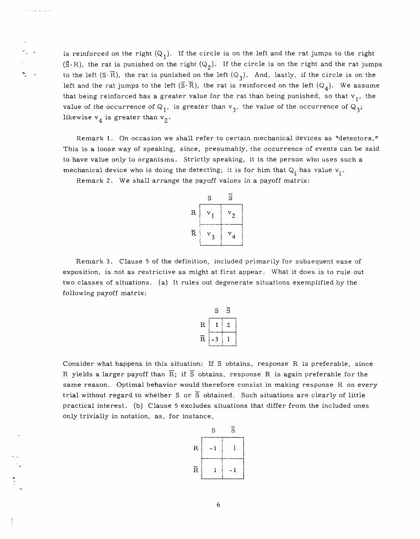
Remark 2. We shall arrange the payoff values in a payoff matrix:

S S

R

R

Remark 3. Clause 5 of the definition, included primarily for subsequent ease of

exposition, is not as restrictive as might at first appear. What it does is to rule out

two classes of situations. (a) It rules out degenerate situations exemplified by the

following payoff matrix:

S S

R 1 Z

R -3 1

Consider what happens in this situation: If S obtains, response R is preferable, since

R yields a larger payoff than R; if S obtains, response R is again preferable for the

same reason. Optimal behavior would therefore consist in making response R on every

trial without regard to whether S or S obtained. Such situations are clearly of little

practical interest. (b) Clause 5 excludes situations that differ from the included ones

only trivially in notation, as, for instance,

S S

R -1 1

R 1 -1

6

If in this matrix we replace S by S and S by S, we obtain a matrix that satifies the

inequalities of clause 5. Excluding such "mirror image" cases enables us to state very

simply what we mean by the accuracy of detection.

Accuracy of Detection. To make response R when S obtains - this is sometimes

called a "hit" - or to make response R when S obtains is, we shall say, to make a

correct response. To make response R when S obtains - this is sometimes called a

"false alarm" - or to make response R when S obtains - sometimes called a "miss" -

is to make an incorrect response. The accuracy of detection in a given situation will,

of course, be measured by the ratio of the number of correct responses to the total

number of responses made in the situation.

If in a given situation the accuracy of detection is a o , we shall say that the detec-

tability of the signal (to be defined later) in that situation is a .

Expected Payoff. If we know the probability of a hit, Pr(RIS), and the probability

of a false alarm, Pr(R I S), in a given situation, we can calculate the expected value of

the payoff according to the following obvious formula:

E(V) = v1 Pr(R IS) Pr(S) + v 2 Pr(R S) Pr(S)

+ v3 Pr(R IS) Pr(S) + v4 Pr(R S) Pr(S) 8)

7

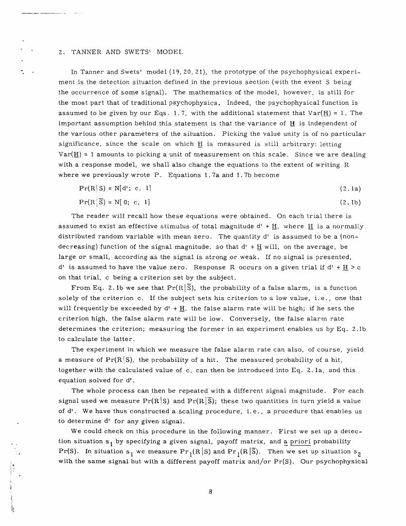
2. TANNER AND SWETS' MODEL

In Tanner and Swets' model (19, 20, 21), the prototype of the psychophysical experi-

ment is the detection situation defined in the previous section (with the event S being

the occurrence of some signal). The mathematics of the model, however, is still for

the most part that of traditional psychophysics. Indeed, the psychophysical function is

assumed to be given by our Eqs. 1. 7, with the additional statement that Var(H) = 1. The

important assumption behind this statement is that the variance of H is independent of

the various other parameters of the situation. Picking the value unity is of no particular

significance, since the scale on which H is measured is still arbitrary: letting

Var(H) = 1 amounts to picking a unit of measurement on this scale. Since we are dealing

with a response model, we shall also change the equations to the extent of writing R

where we previously wrote P. Equations 1. 7a and 1. 7b become

Pr(R| S) = N[d'; c, 1 (2. la)

Pr(RS) = N[ 0; c, 11 (2. lb)

The reader will recall how these equations were obtained. On each trial there is

assumed to exist an effective stimulus of total magnitude d' + H, where H is a normally

distributed random variable with mean zero. The quantity d' is assumed to be a (non-

decreasing) function of the signal magnitude, so that d' + H will, on the average, be

large or small, according as the signal is strong or weak. If no signal is presented,

d' is assumed to have the value zero. Response R occurs on a given trial if d' + H > c

on that trial, c being a criterion set by the subject.

From Eq. 2. lb we see that Pr(RIS), the probability of a false alarm, is a function

solely of the criterion c. If the subject sets his criterion to a low value, i.e., one that

will frequently be exceeded by d' + H. the false alarm rate will be high; if he sets the

criterion high, the false alarm rate will be low. Conversely, the false alarm rate

determines the criterion; measuring the former in an experiment enables us by Eq. 2.lb

to calculate the latter.

The experiment in which we measure the false alarm rate can also, of course, yield

a measure of Pr(RIS), the probability of a hit. The measured probability of a hit,

together with the calculated value of c, can then be introduced into Eq. 2. la, and this

equation solved for d'.

The whole process can then be repeated with a different signal magnitude. For each

signal used we measure Pr(RIS) and Pr(R S); these two quantities in turn yield a value

of d'. We have thus constructed a scaling procedure, i. e., a procedure that enables us

to determine d' for any given signal.

We could check on this procedure in the following manner. First we set up a detec-

tion situation s 1 by specifying a given signal, payoff matrix, and a priori probability

Pr(S). In situation s we measure Prl(RIS) and Prl(RIS) . Then we set up situation s2

with the same signal but with a different payoff matrix and/or Pr(S). Our psychophysical

8

measurements now yield Prz(R S) and Pr(RIS). Since s1 and s2 are different situations,

we find, presumably, that Pr 1 (RIS) * Pr 2 (RIS) and that Prl(R S) Pr 2 (R S). For a

subject behaving optimally, at any rate, these inequalities can be shown to hold. We

now solve Eqs. 2.1, using Prl(R S) and Prl(R S), and obtain a value d' . Repeating

the process, using Pr 2 (R S) and Pr 2 (R S), we obtain d'. Under ideal circumstances,

i. e., if there is no experimental error, we should find that d' 1 = d'2' since both of these

numbers measure the effective stimulus magnitude of the same signal. Unfortunately,

we would need further statistical analysis to determine what discrepancies we could

tolerate, and such an analysis has not, to our knowledge, been developed.

Tanner and Swets' model enables us to relate our uncertainties one to the other.

We can, for example, write the probability of a hit as a function of d' and the probabil-

ity of a false alarm, eliminating the criterion c. The predictive power per se of the

model is not, however, increased thereby. If our interest lies in predicting the psy-

chophysical function, i.e., in predicting the probabilities Pr(RIS) and Pr(RjS) corres-

ponding to a given signal, we still have to know beforehand: (a) the magnitude of our

signal on the effective stimulus scale; and (b) the value of the parameter c. From the

point of view of experimental prediction we have improved on the venerable phi-gamma

hypothesis only to the extent of writing Eq. 2. lb; that is, only to the extent of adopting

the criterion approach of the last section.

We now want to gain some insight into how we can change the false alarm rate with-

out changing the signal. It is essential that we be able to do so in order to have a check

on the scaling procedure just described. Consider the following example.

Example. Let the payoff matrix be

S S

R 100 0

R 0 1

and let Pr(S) = 0.99. In such a situation a clever subject will almost always make the

response R, since if he makes this response he stands a good chance - indeed a 99 to 1

chance -of being paid 100; but if he makes response R, he can at most be paid 1 - and

that much only once in a hundred times. The subject will therefore, presumably, set

his criterion very low so that it will almost always be exceeded by d' + H, and response

This concept is defined below. In order for the inequalities to hold, it is sufficient(in optimal behavior) for the parameter , defined by Eq. 2. 2, to assume differentvalues in situations s and s 2.

Tanner and Swets also show how predictions in the present kind of psychophysicalexperiment are related to predictions in the "forced-choice" experiment. This part oftheir model will not be discussed. The forced-choice situation in general will be dis-cussed in sections 4 and 5.

9

-------- -_-__ --- ·-------.--- ;_1Y_-·_--^L_2 --__·_=__._*·C*. ~*l ~r*---- nIcr

R will be made on almost every trial. Only if the total effective stimulus magnitude is

extremely low will he let himself be convinced that the signal was not presented (that d'

= 0 on that trial) and make response R.

If we change the situation by letting the payoff matrix be

S S

R 1 0

R 0 100

and by letting Pr(S) = 0. 01, the reverse will presumably occur. The subject will now

set his criterion very high and make response R on almost every trial. Only if the

effective stimulus is extremely large, will he take it as evidence that a signal was pre-

sented (that d' 0 on that trial) and make response R.

We see, therefore, that a clever subject will pick his criterion differently in dif-

ferent situations even though the signal remains the same. We might even suspect that

there is an optimal way of picking the criterion so that the expected payoff to the subject

is maximized in the given situation. A subject who sets his criterion to such an opti-

mal value, cmax , would be said to be behaving optimally.

[A subject behaving optimally in the sense of the present discussion must not be

confused with what we shall call an ideal detector. The latter maximizes the expected

value of the payoff. The former maximizes the expected value of the payoff in a situa-

tion in which conditions (1.4) and (1. 5) - the fundamental conditions of the model - hold.

We may say that our optimally-behaving subject is an ideal detector for a situation in

which the information about the signal and the variability ("noise") is available only in

the form stipulated by Tanner and Swets' model.]

While Tanner and Swets themselves do not particularly stress this notion of optimal

behavior, it might be of interest here to investigate it somewhat further. The mathe-

matics of the situation is worked out in Appendix B. Here we merely state the result.

First, a definition:

(v4 - v2) Pr(S)

Let = (v-1 - v3 ) Pr(S) (2.2)

This quantity incorporates the relevant information about the payoff matrix and the

a priori probability of a signal. In terms of the (known) parameter we find that

In d' (2. 3)

max 2d'

10

_ _q_ I _I�____ _··_�___ _I �I _I� I_··I_�_1__11_ � I __ I

Putting this result in Eqs. 2. 1 and rearranging terms, we see that for a subject behaving

optimally the psychophysical function is

d'Pr(R 1 NL0,2 (Z.4a)

In pPr(R S)= 1- N + 0, 1 (2. 4b)

Note that these functions (plotting the probability versus d') are not, in general, in the

shape of normal distributions (normal ogives are obtained only in case = 1). This may

be considered startling when we reflect that our basic equations (2. 1) are, of course,

normal ogives. The difference occurs because the subject behaving optimally changes

his criterion not only with changes in the payoff matrix or the a priori probability but

also with changes in the signal (changes in d'). Thus, the quantities c and d' appearing

in Eqs. 2. 1 are not independent of each other in the case of optimal behavior; insofar as

our subjects approximate such optimal behavior the usefulness of these equations may

therefore be seriously doubted even if the model that led to them is accepted.

In our discussion of the scaling procedure we saw that the two measured probabilities

Pr(R S) and Pr(R S) corresponding to a given signal were necessary to yield an estimate

of d'. We see from Eq. 2.4 that on the assumption of optimal behavior each of these two

probabilities yields an estimate of d'. This provides us with a check for optimal behav-

ior: The experimenter selects a value of , that is, selects a payoff matrix and a Pr(S),

and selects a particular signal to be used. The probability of a hit and of a false alarm

are then measured. Each of these yields an estimate of d'. The two estimates ought to

agree within the tolerance of experimental error if the subject is behaving optimally

(some statistics would again be necessary to determine this tolerance). Unfortunately,

the experiment performed by Tanner and Swets did not follow this straightforward pro-

cedure. Their experiment - which according to our definition is not a detection situa-

tion - was set up so that on each trial there was presented either no signal or one of four

signals differing in magnitude, the payoff matrix being

S 1 S2 S3 S4 S

R

R

It is not clear to us how, fromr

whether or not the subject was

the results of such an experiment, one could determine

behaving optimally.

11

V1 v1 v 1 v 1 V2

V3 V3 V3 V3 V4

3. DETECTION THEORY

[The material for this section is drawn from Peterson and Birdsall (15). The readeris referred to their monograph for further details, proofs, and a short bibliography ofother writings on detection theory. A brief historical introduction to detection theory isgiven in our Appendix J.]

In discussing the models considered thus far we spoke of signals in a very general

way. The specific nature of the signal - its duration, for instance - played no part in

the theorizing. Likewise, the nature of the random variability was hardly analyzed: we

arbitrarily assumed the existence of a single random variable H with normal distribu-

tion and fixed parameters.

A more sophisticated analysis is made in detection theory; it results, as one would

expect, in a model of greater power, although, admittedly, also of greater mathematical

complexity. It is the purpose of this section to present some of the fundamental ideas

of this theory.

The Signal. By a signal, we shall understand a measurable quantity varying in a

specified manner during a fixed observation-interval T seconds long. Letting time be

measured from the beginning of the observation-interval, we may represent the signal

by a time-function s(t) defined on the interval 0 < t < T.

It will be assumed that s(t) is series-bandlimited to a bandwidth W s. By this we

mean that s(t) has a Fourier series expansion on the interval 0 < t < T; that the series

contains only a finite number of terms; and that the frequency of the highest harmonic

is Wss

The Noise. As in previous models, we shall assume that the signal is perturbed

by random variability. Since the signal is now represented by a time-function, we

must let this perturbation occur at each moment of time at which the function is defined.

Mathematically we do this by adding to our signal-function s(t) a "random" time-

function, i. e., a function whose value at each moment of time is specified only in a

statistical sense. Such a function n(t), 0 < t < T, will be said to describe the noise in

the situation. It will be assumed that n(t) is series-bandlimited to a bandwidth W > Ws

Receiver Inputs; the Events S and S. Each observation-interval thus yields a time-

function. Such a function - or its physical counterpart - is called a receiver input. It

is designated by x(t).

By saying that the signal is presented during a given observation-interval, we mean

that the receiver input for that interval is given by

x(t) = s(t) + n(t) 0 < t < T

By saying that the signal is not presented during a given observation-interval, we mean

that s(t) = 0 for that interval, so that the receiver input is given simply by

x(t) = n(t) 0 < t < T

We say that the event S or S occurs according as the signal is or is not presented.

12

In either case the receiver input is given by a series -bandlimited time-function defined

on the interval 0 < t < T; this function is "random" since, in either case, it contains the

"random" term n(t).

The Sampling Theorem. We shall need one form of the so-called sampling theorem

in the time-domain. [For a proof of this theorem see Appendix D of reference 15. Also

compare references 5 and 16.] The theorem states that any fixed time-function defined

on an interval 0 < t < T and series -bandlimited to a bandwidth W can be uniquely repre-

sented by a set of 2TW numbers, these numbers being the value of the function at

"sampling points" 1/2W seconds apart on the time-axis.

Accordingly, if we knew the value of x(t) at each of the ZTW sampling points, we

could reconstruct x(t). The function x(t), however, is a "random" function; its value

at the sampling points is determined only in a statistical sense. Thus, instead of repre-

senting this function by ZTW numbers, as we would in the case of an ordinary well-

specified function, we must use, instead, a set of 2TW random variables, X 1 ,X 2 .. X2TW

On occasion it will be found convenient to denote this set by the single letter Ip".

We have, thus, three equivalent ways of writing a receiver input: x(t); X 1 .XZTW

and .

Probability Density of the Receiver Input. We consider, next, the joint probability

density of the random variables X 1 , . . XZTW. (It is here assumed that the density

exists, i. e., that the joint distribution function of the Xi has all derivatives.) This

density will, by virtue of the sampling theorem, give us the complete statistical speci-

fication of the receiver input.

Actually, it will be found convenient to break up this density into two conditional

densities, one for each of the two cases S and S. The symbol "fSN" will be used to

denote the joint density (of X1, .,X2TW) that obtains in case the receiver input contains

both signal and noise; "f N will be used for the density in the alternative case of noise

alone.

In formal notation we have

Pr(X1 < a1 , X < a . XZTW < aZTW I S)

a 1 a aT w

_SN (xi, ; ..l.Xg I xZTW) dxldxg ' dxZTw

-cc -00 -00

Pr(X1 < a1 , X 2 < a X2T < aT W S)

a 1 a aZTWa1a fN(xl, x, ... , x2T w ) dxldx 2 ... dx2TW

Likelihood Ratio. Recall that the probability density of the receiver input is

fsN(xl ... xZTW) or fN(xl ... XW.. ) according as the signal is or is not presented.

13

We now define the likelihood of the receiver input to be fSN(Xl ... XTWw) or

fN(X1 . ..2 XZTW) according as the signal is or is not presented. In our summary nota-tion, the likelihood is written fSN( ) or fN(T). The likelihood ratio L(4'') of a receiver

input is then defined as follows:

fSN ( X ) fsN(X 1 .... .XZTW)L() fN( ) - fN(Xl ... 2T W)

The likelihood ratio of a particular receiver input tells us, very roughly speaking,

how likely it is that this input contains the signal; if the likelihood ratio is large, we

may take it as evidence that a signal is present; the larger the likelihood ratio, the

weightier the evidence. Since our receiver input is random, we can never, of course,

be sure; some receiver inputs containing the signal and noise will yield low values of

the likelihood ratio, and some containing only noise will yield high values.

The likelihood ratio must not be confused with the ratio

fsN(l ... X2TW)

fN(Xl .. X2TW)

of the densities. The variables occurring in the likelihood ratio, unlike those occurring

in the ratio of the densities, are random variables. The likelihood ratio is thus a func-

tion of random variables, and, like any function of random variables, is itself a random

variable. It is thus meaningful to speak of the distribution of the likelihood ratio, while

it would be nonsensical to speak of the distribution of the ratio of densities, just as it

would be nonsensical to speak of the distribution of a distribution.

As in the case of the receiver-input density, we break up the distribution of the

likelihood ratio into two conditional distributions, one for each of the two cases S and

S. Denoting these distributions* by FSN and F N, we have

FSN(x) = Pr(L(P) > x IS) (3. la)

FN(X) = Pr(L(I/) > x S) (3. lb)

Thus, the expression FSN(D), to be used later, designates the probability that the likeli-

hood ratio of a receiver input containing the signal exceeds the number . The expres-

sion FN(P) designates the corresponding probability for a receiver input containing noise

alone.

To fix our ideas, let us consider the following simple example.

Example: Likelihood Ratio in a Discrete Case. We are given a loaded coin, and

we know, for one reason or another, that the odds are 10 to 1 in favor of a particular

one of the two faces coming up when the coin is tossed, but we do not know which face

Notice the direction of the inequality in Eqs. 3. la and 3. lb. The functions arecomplementary distribution functions, since they give the probability that L(4I) liesbetween x and +oo, rather than between -co and x, as is usual.

14

is favored. We decide to toss the coin once and count the number K (O or 1) of "heads"

that come up. K is our receiver input. We shall say that the event S or S obtains

according as the true probability of heads is 1/11 or 10/11.

Since we are dealing with discrete quantities, we shall write probability distributions

rather than densities. Thus,

fsN(n) = Pr(K = nIS) = ( 1 / 1 1 )n ( 1 0 / 1 1 )1- n (3. a)

fN(n) = Pr(K = n S)= ( 1 0 /11)n ( 1 / 1 1 )1n (3. 2b)

(n = 0 or 1)

The likelihood ratio is

fsN(K) (1/1 ) (10/) 1-2L(K) = = 10 - K (K = 0 or 1)

fN(K) )K 1-K

The likelihood ratio is thus seen to be a simple function of the random variable K.

It is itself a random variable and has a probability distribution. Let us calculate this

distribution for the case in which S obtains; that is, let us calculate

Pr(L(K) = mlS) = Pr(10l2K = mIS) (m = 1/10 or 10)

Replacing the expression 1 0l K - m by the equivalent expression K = (1 - log m)/2, we

have

Pr(L(K) = mlS) = Pr = og m2

Replacing n in Eq. 3. 2a by (1 - log m)/2 we obtain our result

1-log m 1-log m

Pr(L(K) = mIS) = (1/11) 2 (10/11) 2 (m = 1/10 or 10)

By a similar argument we can obtain

1-log m 1-log m

Pr(L(K) = m|S) = (10/11) 2 (1/11) 2

We see, therefore, that the random variable L(K) assumes the values 1/10 and 10,

respectively, with probabilities 1/1 1 and 10/11 if S obtains, and with probabilities

10/11 and 1/11 if S obtains.

A Fundamental Theorem of Detection Theory. Consider a detection situation as

defined in section 1, with given payoff matrix and Pr(S), and with the event S defined to

be the occurrence of a given signal; and consider the following Decision Procedure: For

any receiver input make response R if and only if L(T ) > p, where is given by Eq. 2.2.

15

-------^mrr�.r-��-m�-?r*�n��*·PT·13RSLI

Theorem. A detector behaving in accordance with the decision procedure maxi-

mizes the expected value of the payoff in the given detection situation.

Conversely, a detector maximizing the expected value of the payoff in

the given detection situation makes the same responses as one behaving

in accordance with the decision procedure.

[For proof, see Peterson and Birdsall's Theorems 1 and 2, section 2.4. 2 (ref. 15).]

A detector behaving in accordance with the decision procedure will be called "an

ideal detector". For an ideal detector we see that

Pr(R!S) = Pr(L(/) > IS) = FSN( ) (3. 3a)

Pr(R S) = Pr(L(4) > S) = FN(O) (3. 3b)

Continuation of the Preceding Example. Suppose that on the basis of our toss of the

coin, i. e., on the basis of K, we are required to choose between response R and R.

Suppose, moreover, that we are given that Pr(S), the probability that the coin is biased

toward tails, is 1/12, and that the payoff matrix is

S S

R 1 -1

R -1 1

With this payoff matrix and this value of Pr(S) we find that = 11, and the fundamental

theorem tells us to make response R if and only if L(K) > 11. In the present example,

however, the likelihood ratio never exceeds 10, as we have already seen. Thus,

Pr(R IS) = Pr(R S) = 0. The expected value of the payoff in this case is 10/12 = 0. 82,

as may be established by substitution into Eq. 1. 8.

Suppose that we pick a decision procedure not in accordance with the fundamental

theorem. Thus, for example, suppose that we decide to make response R if and only

if L(K) > 1. We have already calculated that the probability of this event is 10/11 in

case S obtains, and 1/11 in case S obtains. Thus, Pr(RIS) = 10/11 and Pr(RIS ) = 1/11.

Putting these values into Eq. 1. 8 we find that the expected value of the payoff is now

reduced to 49/66 = 0. 74.

We thus see that in ideal detection the critical quantities are the distribution func -

tions FSN and F N of the likelihood ratio of the receiver input. Fortunately, Peterson

and Birdsall (15) have calculated these functions for a wide variety of signals presented

in uniform gaussian noise. We can introduce their results directly into Eq. 3. 3 to

*By a uniform gaussian noise we mean a time-function whose distribution of

instantaneous amplitudes is gaussian (normal) and whose power-spectrum is uniformover a given range and zero outside that range.

16

obtain the psychophysical function for the ideal detector. If the signal is known exactly,

as it would be with a pure tone of known amplitude, frequency, and phase, we obtain

Pr(R S) = 1 - N - d- 0, (3.4a)

Pr(R IS) = 1 - N0 + ; 0, (3.4b)

where

2 ZEd =N '

E being the signal energy (the signal power multiplied by T), and

E being the signal energy (the signal power multiplied by T), and No being the noise

power per unit bandwidth (cps).

We notice, incidentally, that if we write d' for d in the expressions above, we obtain

Eqs. 2.4, which, it will be recalled, hold for the case of optimal behavior on Tanner and

Swets' model. The difference is that in the present equations the variable d is measured

in actual physical units, while in Tanner and Swets' situation the variable d' is measured

on an unknown scale of effective stimulus magnitudes. It may be added, parenthetically,

that if we had chosen a somewhat different situation - for example, one in which the

signal had unknown phase - we would have obtained an entirely different set of functions

for Pr(R S) and Pr(R S).

The two probabilities Pr(R IS) and Pr(R IS) may, of course, be combined into a single

quantity, the probability Pr(C) of a correct response, or detectability, as defined in

section 1. The formula for doing so is, obviously,

Pr(C) = Pr(RIS) Pr(S) + Pr(RIS) Pr(S) (3.5)

The detectability function for the case of the signal known exactly may be found by sub-

stituting the expressions for Pr(RIS) and Pr(RIS) from Eqs. 3.4 in Eq. 3.5. The

resulting function with Pr(S) set to 1/2 is plotted in Fig. 1 for several values of p.

We have seen in a general way how the ideal-detector psychophysical function for a

particular kind of signal and of noise can be obtained. Let us examine this result. It

has already been remarked that, in the present case, unlike that of optimal behavior on

Tanner and Swets' model, there is no uncertainty about scales. We notice, moreover,

that the effect of changing the duration of the signal is immediately given by Eqs. 3.4.

For instance, we see that increasing the signal duration and decreasing the signal power

by a given factor leaves everything unchanged. This is the so-called I-T Law of psycho-

physics, which is found to hold within limits (11). The equations also predict constant

detectability for constant signal-to-noise ratio, other things being equal; this, too

is found to hold within limits in auditory experimentation (11). Furthermore, the

equations show that for an ideal detector the detectability is independent of the noise

bandwidth; auditory experiments reveal that this is the case for human subjects, again

within limits (11).

17

'`�r� - ---- r*r)p�-

1.0

0.9

0.8

J 0.7

aow

0.6

0.5

Pr (S)-

0.04 0.06 0.1 0.2 0.4 0.6 1 2 4 6 10 20

E/N o

Fig. 1. Ideal-detector psychophysical functions. Signalknown exactly; Pr(S) = 1/2. ("Yes-No ' situation.)

Aside from these (perhaps accidental) facts, we might ask what relevance this kind

of model has, in general, to empirical psychophysics, knowing, as we do in advance,

that no subject is an ideal detector. First of all, the model allows us to place lower

bounds on our threshold measurements. For example, we see from Fig. 1 that for a

signal known exactly, a uniform gaussian noise, and Pr(S) = 1/2, the detectability can-

not exceed 0. 76 if the signal energy does not exceed the noise power per unit bandwidth.

In similar fashion, lower bounds can be set for a wide variety of situations. Second,

establishing the manner in which and the extent to which a subject's behavior differs

from that of an ideal detector might lead to interesting insights into sensory psychology.

If, moreover, the difference between subject and ideal detector is found to be expressible

in terms that are sufficiently simple, we might be able to generate, by simple additions

to the present model, a powerful tool for the prediction of actual behavior.

18

_1__ _____1___11__111_____ 1 -� _���---·--·1111�·11111�·111111�·�

4. PROBLEMS OF EXPERIMENTAL TECHNIQUE AND THE FORCED-CHOICE

METHOD

A basic problem concerning the payoff matrix has thus far been avoided. Recall

that the v i are the values, for the subject, of various events in the detection situation.

How are we to determine these values ? To be sure, the experimenter may try to assign

the values by using a system of monetary rewards and fines. There is no guarantee,

however, that the value for the subject corresponds to the number of cents involved; the

value of two cents may be different from twice the value of one cent.

Moreover, the various events in the detection situation may have "private" values

for the subject, prior to or independently of the assignment of values by the experimenter.

Thus, in a particular experiment we might have:

Q2 : subject is fined $1 upon making response R when S obtains (i.e., upon makinga false alarm);

Q 3: subject is fined $1 upon making response R when S obtains (i.e., upon missing

the signal).

Even though the money involved in Q 2 and Q3 is the same, the amount of displeasure

experienced by the subject may be quite different in the two cases. If Q3 occurs, the

subject may reflect that he has made response R (which is appropriate to trials on

which there is no signal, since in that case it earns $1) on a trial on which there was a

signal; but after all, no one is perfect, the signal was very weak, etc., ... On the other

hand, if Q 2 occurs, he may reflect that he has made response R (appropriate to trials

on which there is a signal) on a trial on which there was no signal; the experimenter

may think he is having hallucinations, perhaps there is something wrong with his sense

organs, etc .... If the subject has such feelings, the values of Q2 and Q 3 will be quite

different.

It would be excellent, therefore, if we could get along without the v. altogether.1

This we cannot do. We can, however, take a step in that direction with the help of the

following result.

It is easy to show (see Appendix C) that the maximum expected payoff is independ-

ent of the v. so long as1

v1 = V4 and v 2 = v 3 (4. 1)

A payoff matrix for which Eq. 4. 1 holds will be called symmetrical.

Thus, if a subject is instructed to try to maximize the values that accrue to him,

his task, and therefore presumably his behavior, will be independent of the payoff

matrix, so long as the latter is symmetrical. Instead of having to worry about four

quantities, therefore, we need worry only about the symmetry of the payoff matrix.

*Strictly speaking, these instructions are unnecessary, since what we presumably

mean by "value" is "something which people try to maximize."

19

____� �__I^I___I__�_IIIIYL_�·I�-�PI1·-L�·-�-�

As our discussion has just shown, however, the kind of experimental situation we

have been considering is basically asymmetrical: Q 2 and Q3- or Q1 and Q4, for that

matter - are psychologically different and may therefore have intrinsically different

values for the subject. It is felt that condition (4. 1), if not totally satisfied, can at

least be approximated better in an experiment using the so-called (temporal) two-

category forced-choice technique.

The experimental technique implicit in our discussion thus far has been the :'yes-no"

method. We are using this method whenever we set up our experiment as a detection

situation in accordance with the definition of section 1, interpreting the event S of that

definition to be the occurrence of a signal (as defined in section 3). Thus, on each trial

of a yes-no experiment there is an observation-interval during which the signal may

occur.

In the two-category forced-choice method there are on each trial two observation-

intervals, during one and only one of which the signal occurs (whether on a given trial

the signal occurs during the first or second observation-interval is determined, of

course, at random); the noise (if any) occurs in both observation-intervals. Otherwise

the forced-choice and the yes-no experiments are identical.

The forced-choice situation, it will be observed, fits our definition of a detection

situation if we interpret the event S of that definition to be the occurrence of a signal

in the first observation-interval (with the event S consequently to be interpreted as the

occurrence of a signal in the second observation-interval).

In order for the notation to be indicative of the kind of experiment being discussed,

the symbols S, S, R, and R, will be reserved for the yes-no situation, and the symbols

S:S (signal in the first interval, no signal in the second), S:S, R 1, and R 2 will be used

for the corresponding events in the forced-choice situation.

The objectional kind of asymmetry found in the yes-no technique is not present to

such an extent in the forced-choice technique. We may set up the following forced-

choice situation, where, to emphasize the symmetry, we let the subject indicate his

responses by pushing a switch to the left or right:

Q1 : subject is paid D dollars upon receiving the signal in the earlier observation-

interval and pushing the switch to the left;

Q 2: subject is fined D' dollars upon receiving the signal in the later interval and

pushing the switch to the left;

Q 3 : subject is fined D' dollars upon receiving the signal in the earlier interval and

pushing the switch to the right;

Q4 : subject is paid D dollars upon receiving the signal in the later interval and

pushing the switch to the right.

Except for an interchange of "earlier" with "later" and of "left" with "right," our

descriptions of Q1 and Q 4 , and of Q2 and Q 3, are identical. In order for Eq. 4. 1 to

hold, therefore, we need only assume that such temporal and spatial differences do not

affect the values that the subject places on the events.

20

_ ___~~~~~~~~~~~~~~~~~~~~~~~~~~~~~ I(_��·I_· I _L_ _�I_ �_1__ �11__(__1(__~~__I~~ U ~ ~ ~ ~__~ ~ _·___~~~~_11I_·~~~__I__I_ ~ I--

If this assumption is true, i. e., if the value of Q1 equals that of Q and the value of

Q2 equals that of Q3, then our previous result tells us that it is immaterial what the

actual values are. For that matter, the monetary values D and D assigned by the

experimenter are also immaterial; we may replace the event of being paid D dollars

by a flash of green light, for example, and the event of being fined D' dollars by a

flash of red light, with the understanding that the green light is "correct" or 'good,;'

while the red light is "incorrect" or bad.l Our instructions to the subject may then

simply be to try to maximize the occurrence of flashes of the green light.

In order to complete the symmetry of the situation we may want to set

Pr(S:S) = Pr(S:S) = 1/2 (4. 2)

A forced-choice situation in which both Eqs. 4.1 and 4.2 hold will be called a"symmet-

rical forced-choice situation. T

21

�-------�� -�-------C- -I*�---r�--��-�--·-----·�rr�;-i--nr�.?�- Lv"C-�*Crr*l·l·la�-r�--�·ra�·

5. IDEAL DETECTION IN A TWO-CATEGORY FORCED-CHOICE SITUATION

Let us consider a signal s(t) and a noise n(t), as defined in section 3. Since we are

dealing with a forced-choice situation, we shall have two observation-intervals and,

hence, two receiver inputs, xl(t) and x 2 (t). If xl(t) = s(t) + n(t) and x 2 (t) = n(t), we say

that S;S obtains; if x l (t) = n(t) and x2 (t) = s(t) + n(t), we say that S:S obtains. Either

S:S or S:S must, of course, obtain on a given trial.

We have already seen how a receiver input may be considered to be a set ' of 2TW

random variables. Two such sets, ' 1 and , will be necessary here, to correspond

to the two receiver inputs xl(t) and x2 (t). Notice that on any given trial one of the two

quantities, 1 I2' has the density fSN and the other the density fN'

The payoff matrix for the forced-choice situation is written

S:S S:S

R1

R2

where v1 > v 3, and v 4 > v2 . Corresponding to our earlier definition, we have

(v 4 - v 2 ) Pr(S:S)= (5.1)

(v 1 - v 3 ) Pr(S:S)

We now need a decision procedure for ideal detection in the forced-choice situation

to correspond to the one in the yes-no situation. (See section 3, Fundamental Theorem

of Detection Theory.) It is shown in Appendix D that the desired rule is as follows.

Decision Procedure for Ideal Detection in the Forced-Choice Situation. Make

response R1 if and only if L(' 1 ) > L(\I/), where the likelihood ratio is defined as

before.

This provides the general solution. From it we can calculate solutions for particu-

lar cases as was done in a previous section for the yes-no experiment. Ideal-detector

psychophysical functions are derived in Appendix E for two kinds of signals presented

in uniform gaussian noise: (a) signals known exactly; (b) signals known except for

phase (the strict definition of the kind of signal considered here is given by Eq. E. 14

of Appendix E).

Case of the Signal Known Exactly. From Appendix E, Eqs. E. 12 and E. 13, we

have

Pr(R1 i S:S) = 1- N[ n h ; 0, 1] (5. 2a)

Pr(R1 S:S) = 1 - N [ h + ; 0, 1] (5. 2b)h 2~~

22

where

h 2 - 4EN

It is interesting to compare these equations with the corresponding equations (3.4a

and 3. 4b), for the yes-no situation. It will be seen that if the signal-to-noise ratio,

E/N o, in the yes-no situation is made twice as great as in the forced-choice situation,

the psychophysical functions become identical.

Equations 5. 2a and 5. Z2b may be combined into a single detectability function by

means of the following obvious formula:

Pr(C) = Pr(R1 S:S) Pr(S:S) + Pr(R2 I S:S) Pr(S:S)

where Pr(C) is the probability of a correct response.

If = 1 and Pr(S:S) = Pr(S:S) = 1/2, the detectability function is

Pr(C) = N ) ; 0, 1

This function is plotted in Fig. 2.

1.0

0.9

0.8

-

I-0U

0

0.7

0.6

0.5

(5. 3)

(5. 4)

Pr (S S)= 2

PHASE

0.02 0.04 0.06 0.1 0.2 0.4 0.6 1 2 4 6 10

E/No

Fig. 2. Ideal-detector psychophysical functions for the two-category forced-choice situation. Signal known exactly and known except for phase;p = 1; Pr(S:S) = 1/2.

23

Case of the Signal Known Except for Phase. This case is solved in Appendix E for

3 = 1 only. From Eqs. E. 29 and E. 27 we have

Pr(R1 S:S) = - exp L-2N J (5. 5a)

Pr(R1 | S:S) = exp -2N o (5. 5b)

Combining these two equations into a single detectability function by formula 5. 3 we

have, for Pr(S:S) = Pr(S:S) = 1/2 (and 1 = 1),

Pr(C) = 1 - exp - 2 (5.6)

This equation is plotted in Fig. 2.

We have already discussed the advantages of the detection-theory model as it applies

to the yes-no situation (section 3). Our comments apply equally well to the present

forced-choice situation.

24

___. _I_ �I·_

PART II. EXPERIMENTAL RESULTS AND DISCUSSION

6. INTRODUCTION

The experiments discussed in this report were undertaken with the aim of exploring

the manner in which and the extent to which a human subject differs from an ideal detec-

tor in the performance of an auditory detection task.

The two-category symmetrical forced-choice technique was used throughout. For

a discussion of this technique and its advantages the reader is referred to Part I, sec-

tion 4.

Two experiments were performed in order to measure with a considerable degree of

accuracy the subjects' ability to detect auditory signals in the presence of broadband

gaussian noise. Experiment 1 dealt with sinusoidal signals. Experiment 2 dealt with

signals having two sinusoidal components. All listening was monnaur.

25

*· -- -*·rai�l�*··e�n*l-r.rlmanarr*�·pl�r?--r

7. DESCRIPTION OF THE EXPERIMENTS

7.1 DESIGN

Signals. The experiments consisted in the measurement of the detectability of

auditory signals in the presence of noise. In Experiment 1 the signals were sinusoids

of known level and frequency but unknown phase. Two frequencies were used: 500 cps

and 1100 cps. At 500 cps, 21 levels - 1 db apart - were selected in such a way as to

cover roughly the range of detectability from 0. 5 (chance) to 1. 0 (perfect detectability).

Similarly, at 1100 cps, 19 such levels were chosen.

In Experiment 2 each signal was composed of two sinusoidal components of the kind

used in Experiment 1. Three pairs of frequencies were used: 500-540 cps, 1060-1100

cps, and 500-1100 cps. For each of the component frequencies three levels, labeled

"soft", "medium", and "loud", were selected. The attempt was made to set these levels

in such a way that soft components were poorly detectable, loud components were highly

(though less than perfectly) detectable, medium components being somewhere in between.

Since, however, these settings had to be made in advance of the experiment, an element

of guesswork was involved. For each pair of frequencies the following five pairs of

levels were used: loud-loud, medium-medium, soft-soft, loud-soft, soft-loud.

In addition to measuring the detectability of the two-component signals, it was also

necessary to measure the detectability of each component taken by itself. For compo-

nents of 500 cps and 1100 cps these measurements fall within the plan of Experiment 1.

It remains, then, for Experiment 2 to measure the detectability of sinusoids of 540 cps

and 1060 cps at each of three levels.

In Experiment 1, forty sinusoidal signals were used; in Experiment 2, six sinusoidal

and fifteen complex signals were used. All in all, then, the detectability of each of 61

signals was measured.

To make results directly comparable, the two experiments were run concurrently,

in the sense that the measurements in Experiment 1 were interspersed with those in

Experiment 2. The specific manner in which this was done is explained in section 7.2.

The exact electrical specification of signal levels is given in section 7.4.

Noise. The masking noise was identical in level and power spectrum for all 61

signals. It was considered by the subjects to be "moderately loud". For exact speci-

fication see section 7.4.

Duration of Signal. The duration of each of the two observation-periods of the

forced-choice trial was 1 second. During one or the other of these periods the signal

was always present; the noise, of course, was present during both. Thus, on each trial

*For theoretical reasons discussed below it was necessary for the noise spectrumto be "reasonably flat" in the neighborhood of the signal frequencies. This entailsstaying in that part of the spectrum in which the earphone frequency-response is flat,i. e., in the lower part of the audio range.

26

the signal was presented for 1 second.

Subjects. All measurements were replicated on each of two subject (HF and PFL).

Both were male students at the Massachusetts Institute of Technology. They were paid

for their services.

7.2 PROCEDURE

The interest in the present experiments lay in measuring the detectability of signals

whose characteristics, except for phase, could be considered known. To approximate

this condition as closely as possible two devices were used. (a) The experiment was

broken up into a succession of runs of 180 trials, with rest pauses between runs. Sig-

nals occurring during a given run differed from one another only in phase; the subject

was thus able to become "set" for a given intensity and frequency. Furthermore the

first 18 trials of a run were not recorded; these trials served the function of allowing

the subject to become acquainted with the noise and with the particular signal used in

the run. (b) At the beginning of each trial a short preview of the signal was presented

in the absence of the masking noise. The subject was thus constantly reminded of the

signal characteristics.

The duration of a trial was 3 1/3 seconds, a run of 180 trials thereby lasting 10

minutes. Each trial was divided into four consecutive periods. (Period 1): A period

lasting 1/3 second during which the signal-preview was presented. (Periods 2, 3): Two

consecutive observation-intervals, each lasting 1 second, during each of which masking

noise was presented, and during one of which the signal was also presented. We speak

of the occurrence of the event S:S or S:S on a given trial according as the signal on that

trial occurred in period 2 or 3. Which of these two events occurred on a given trial

was determined at random, with Pr(S:S) = Pr(S:S), the events being independent from

trial to trial. (Period 4): A response and payoff period lasting 1 second. During this

period the subject indicated his response by pushing a lever switch left or right of center,

causing either a green or a red indicator light near the lever switch to flash. We speak

of the occurrence of the event R 1 or R 2 according as the switch was pushed to the left

or right.

A response was considered correct if either S:S and R 1 or S:S and R 2 occurred; it

was considered incorrect if either S:S and R 2 or S:S and R 1 occurred. The green or

red light flashed according as the response was correct or incorrect.

The subject's task was to try to maximize the number of correct responses, or,

equivalently, of flashes of the green light.

All measurements were repeated a number of times, i. e., each signal was used on

a number of runs. Per subject there were (on the average) six runs to each signal in

Slight differences in the number of runs per signal were arranged with a view to asomewhat complicated statistical analysis of the data. This analysis proved morelengthy than rewarding and was abandoned.

27

��arrurmnnrr-r,�--.r. r i···,rxrrraao·--rr* Cnrmmirr�·�F1"··�l;ClrC·II�.�*·-�--*lr

Experiment 1 and eight runs to each signal in Experiment 2. The particular signal

used on a given run was selected at random. In all, 810 runs were made.

During the entire duration of each run a low-intensity background noise was pre-

sented to mask possible switching transients.

7.3 APPARATUS

During a run the subject wore earphones (Permoflux PDR-8) in sponge-neoprene

cushions (MX-41/AR). Since the listening was monaural, only one of the phones was

connected.

Responses were made on a response box, held in the subject's lap. On the top of

this box were mounted, in addition to the response switch and the two indicator lights

already discussed, three period-indicator lights and the start button. Period-indicator

1, 2, or 3 was lit according as period 1, 2, or 3 of the trial was in progress. The start

button started the run, which ended automatically after 180 trials.

Signals were generated by means of two oscillators (Krohn-Hite 430-A). Care was

exercised in setting the two frequencies (in the case of two-component tones) to be the

requisite number of cycles per second apart: a signal was generated whose frequency

was equal to the frequency-difference of the two components; this signal was then com-

pared by the Lissajous technique with the output of a third oscillator set to the desired

difference.

Noise with flat power-spectrum (up to a cutoff at 20 kc) was provided by a noise

generator (Grason-Stadler 455-A).

Appropriate audio amplifiers, linear adders, and attenuators were used for adding

the signal components to one another and to the noise.

The timing of the various events was performed by a rotary mechanical timer of

period 3 1/3 seconds, and associated relays. Runs were programmed in advance on a

teletype tape, so that the sequence of events during a run was generated automatically.

Four electrical counters were used to count the frequency of occurrence during a

run of the four joint events S:S' R 1, S:S R 1, S:S · R, and S:S R 2.

7.4 ELECTRICAL MEASUREMENTS

Levels (unless otherwise stated, all levels are given in decibels re 1 volt rms)

were measured directly across the phone with a self-calibrating "True RMS" voltmeter

(Ballantine Laboratories Model 320). These readings, which are accurate to approxi-

mately 0. 1 db, will in many cases be sufficient for the statement and discussion of our

results. In some instances, however, we shall need to know the signal to noise-

spectrum-level ratio. Knowledge of this ratio is limited by the inaccuracy of our noise-

spectrum-level measurements; the latter may be taken as correct only to approximately

0.8 db.

28

Signals. The twenty-one 500-cps signals of Experiment 1 ranged in 1-db steps

from -64 db to -44 db. The nineteen 1100-cps signals ranged in 1-db steps from -61 db

to -43 db.

It will be recalled that in Experiment 2 we dealt at each of four frequencies with

sinusoids at three levels: loud, medium, and soft. For a given frequency these three

levels were 3 db apart. The levels for the "loud" sinusoids were -49 db at 500 cps and

-50 at 540 cps. For subject PFL, the level for the "loud" sinusoids at 1100 cps and

1060 cps was set at -46 db; for subject HF, at -48 db. Thus, for example, the signal

designated by "loud 500 cps, soft 1100 cps" consisted, for subject HF, of the sum of

two sinusoids, 500 cps at -49 db, and 1100 cps at -54 db.

Noise. The same masking noise, having a voltage-level across the phone of -19 db,

was used on all runs. The background noise present throughout each run was set at

-41 db.

Noise Spectrum-Level. The noise spectrum-level is given by 10 log 10 No , where

No is the noise power in a band 1 cps wide. This quantity may be calculated from the

output of a calibrated narrow-band filter placed in parallel with the earphone. On the

basis of nine such measurements, made with different filters and different passbands,

the noise spectrum-level was found to be (to approximately 0.8 db) -66 db in the neigh-

borhood of 500 cps and 1100 cps.

Sound Pressure-Level. From the phone calibration we find that, for sinusoids,

the sound pressure-level in decibels re 0. 0002 dyne/cm2 can be obtained approximately

from the voltage-level by adding 113 at 500 cps and 112 at 1100 cps.

29

f:

8. EXPERIMENT 1: RESULTS

The results of Experiment 1 are given by the data points in Fig. 3.

In Part I, Eq. 5. 6, the psychophysical function for an ideal detector operating under

what are roughly the conditions of the present experiment was seen to be

Pr(C) = 1 - exp[ 2N] (8. 1)

where, it will be recalled, Pr(C) is the probability of a correct response, or detecta-

bility; E is the signal energy; and No is the noise power per unit bandwidth. Since we

shall want to use the decibel notation, let us define the signal-energy to noise-spectrum-

level ratio, r, to be 10 log1 0 (E/No). Equation 8. 1 can then be written as

Pr(C) = 1 -2 exp ] (8.2)

In order for this equation to hold, it is necessary, first of all, that I = 1 (see

Eq. 5. 1, section 5). Since we set Pr(S:S) = Pr(S:S), this reduces to the requirement

that the payoff matrix be symmetrical. The extent to which this requirement can be

considered to be fulfilled has been discussed in section 4.

For the equation to apply it is necessary, moreover, that the noise be (a) gaussian,

(b) series-bandlimited, (c) uniform in spectrum-level over the band, and (d) of known

spectrum-level; and that the signal be (e) series-bandlimited, (f) of known energy,

(g) of known frequency, but (h) of unknown phase.

Conditions (a), (b), and (e) were obviously met. Owing mostly to the earphone

characteristic, condition (c) was not met. Suppose, however, that a narrow -band filter

centered at the signal frequency had been inserted into the circuit ahead of the phone.

It is known in psycho-acoustics (3, 4, 18) that the detectability of a signal in noise is

independent of the noise bandwidth so long as the latter exceeds a so-called critical

bandwidth of less than 50 cps (in the lower part of the audio range). From the char-

acteristics of our circuit it is safe to assume that within such a narrow band the

spectrum-level of our noise was very nearly uniform, i. e., the spectrum was very

nearly flat. The insertion into the circuit of our hypothetical filter set to a bandwidth

of 50 cps would therefore (a) leave our data unchanged, and (b) lead to behavior on the

part of an ideal detector as specified by Eq. 8. 2, provided the remaining requirements

are met.

It seems intuitively evident that condition (h) is fulfilled: slight inaccuracies in the

timer and frequency-drift in the oscillator contribute toward randomizing the phase.

(Even without this, our signals ought probably to be considered as being of unknown

phase from the point of view of a human subject.)

The only remaining requirements are that the noise level and the signal energy and

frequency be known. These requirements were, it is hoped, approximated as closely

30

X--- �I����---���---1�-i-·�-·Ic--�lr r·rm�l-�r-rr�*rr�ar�T1I-rClu·r�raarplCIW

c CQcl

1 ,O.

C:

Q0

> .; , n tl L

0 ( ) coW ,- (0 " ) _ W- 0 o 0 0 0 o 0 6 6n0 0

o o cr- r, L .~1 x a

O 0) co r- D 0 W' o r- ,( t

- o O o o 0 - O O 0 O

A118I1VO3130

z

CC0) Qcd Co.O,-'

m =

.,-

(0

31

m

rt,-I

-LJuj

2

0wa-

Lic(6cn0zo

0I)zLO(n

r11

r.l _

. W~~~~~~~~~~~~~~u

as possible by our experimental conditions, as discussed in section 7. 2.

We have established, then, that our ideal-detector function may reasonably be com-

pared with our data.

As the first item of comparison we notice, and this comes as no surprise, that our

subjects were not ideal detectors. The ideal detector operates with 75 per cent accu-

racy when r = 1. 4. For our subjects to detect with the same accuracy we must have r

approximately equal to 15; that is, we must increase the signal-to-noise ratio by

approximately 13.5 db.

Aside from the question of absolute sensitivity, how do our subjects compare with

the ideal detector? Let us take the ideal-detector's psychophysical function (Eq. 8. 2)

and displace it in toto to the right along the r-axis until the curve best fits" the data-

points. In other words, let us compare the subjects' psychophysical function for our

situation with the ideal-detector's function for a situation in which either the signal

energy is reduced or the noise power increased. This procedure yields the solid curves

of Fig. 3. The ideal-detector's function was displaced by the amounts given in column 2

of Table 1. (These values are, of course, only as accurate as our noise spectrum-

level measurements. The significance of column 3 is explained in section 9.)

TABLE 1

1 2 3

Curve Displacement Associated hypothetical(cps) (db re ideal detector) bandwidth

(cps)

PFL: 500 11.6 14

1100 14. 5 28

HF: 500 13 20

1100 15 32

The fit of these curves may be considered quite satisfactory; the best-fitting curve

(PFL:500 cps) accounts for 99.3 per cent of the variance in the graph; the worst-fitting

curve (HF:1100 cps) accounts for 97.3 per cent. (The curves were fitted by eye. Had

a least-squares method for fitting the curves been applied, the percentage of variance

accounted-for could only have increased.)

The argument could be made that the obtained fit is not surprising; the observed

psychophysical functions, like most such functions, are roughly in the shape of a normal

ogive; any reasonable theory would predict curves approximately of this general shape;

all such functions could be made to fit our data fairly well. Such an argument would,

however, be misleading. It is true that our data, when plotted on a decibel scale, look

very much like, let us say, normal ogives. On a different scale the data would have a

different appearance; our theoretical curve would then, however, also change

32

_C_ 1_1� -11_111_--111111--

�-1_11___11_1�1_-_1 11 --1�L1

correspondingly; there is no ambiguity here concerning the scale on which to plot the

data in order for them to fit the model. This fit, moreover, is accomplished by

adjusting a single parameter, in contrast with the ordinary two-parameter normal-ogive

:. - fit. In the language of traditional psychophysics we may say that the present model

predicts the scale and the slope of the psychophysical function. (A quick statistical

test, worked in Appendix F, may even convince us that our theoretical curves fit better

than normal ogives.)

33

BL. _ -- ----LI----�m. --�·-- - --·

9. EXPERIMENT 1: DISCUSSION

On the basis of our results thus far we can conclude that our subjects differed from

the ideal detector only to the extent of being, on the average, 13. 5 db less sensitive at

the frequencies tested. How do we account for these 13. 5 db?

We might consider the hypothesis that the 13.5 db difference is due to the internal

noise of the subject. Assume, first, that the two kinds of noise, internal and external,

are linearly additive; we should then expect the internal noise to become less and less

important, and the difference between our subjects and the ideal detector to diminish

rapidly, as the external noise level is raised. It is well known in psycho-acoustics,

however, that subjects will detect signals with constant accuracy over a wide range of

noise levels if the (external) signal-to-noise ratio remains constant (8); the same, of

course, is true for the ideal detector at all noise levels, as is seen from Eq. 8. 2. We

know, therefore, that if we repeated our experiment with a noise of higher level, we

should arrive again at a figure close to 13. 5 db. This refutes the hypothesis of linearly

additive internal noise.

If we still wish to explain the 13. 5 db on the basis of internal noise, we must postu-

late that the addition is nonlinear. It is possible to speculate, for instance, about

"automatic volume control" of the input to the auditory detector. While it is likely that

such a hypothesis could be worked out in plausible fashion, we shall not try to examine

it here. Instead, we turn to speculations that have the advantage of being considerably

more familiar to workers in psycho-acoustics and also of being more useful in our dis-

cussion of the second experiment.

The fact of constant signal-to-noise ratio for a given detectability and the results

of Experiment 1 lead us to conjecture about an auditory mechanism which is somehow

like the ideal detector except for multiplying the noise power by a constant. For, con-

sider that we install at the input of the ideal detector a mechanism which multiplies the

noise power by 22. The noise-level reaching the detector would then be 13. 5 db higher

than the level of the presented noise, and the ideal detector would behave approximately

as our subjects did; and the requirement of constant detectability for constant signal-

to-noise ratio would be satisfied by virtue of Eq. 8. 2.

Such a noise-multiplying mechanism is not hard to come by, if we are willing, for a

moment, to be quite vague. Suppose that we could think of our ideal detector as being

essentially a bandpass filter (the "ideal filter"). Our data could then be generated by

a detector consisting of a filter like the ideal filter except for having a passband approxi-

mately 13. 5 db wider. *For the output of this filter would be like that of the ideal filter

except that the total noise-power output would be 13.5 db greater.

*A band of frequencies f cps wide is said to have a bandwidth in decibels (re 1 cps) of10 logl0 f. The power in a band of uniform noise is given by the sum of the noise spec-

trum-level (i.e., the power in decibels in a 1-cps band) and the bandwidth in decibels.

34

- -·I - I I ~ ~~ ~~~ ~~~- IrI

Such an ideal filter is indeed specifiable. It is shown by Peterson and Birdsall (ref.

15, Part II, p. 20) that for the kind of signal and noise under consideration a filter having

impulse response

cos [a(T-t)] 0 < t < Th(t) = (9. 1)

0 otherwise

where a is the signal frequency and T is the duration, has an output whose envelope at

time T is related to the likelihood ratio L(P) of the input by a known monotonic function.

The filter specified by Eq. 9. 1 could therefore form the basis of an ideal detector.

When T is large compared with a period of the signal - and this is the case with the

signals of Experiment 1 - the gain-versus-frequency characteristic of the ideal filter is

approximately of the form shown in Fig. 4; the larger T, the more peaked and narrow

the graph.

Assume that the ideal filter is centered at the frequency of the signal. If the filterhon__xririt4-4.4 + nerP>Cod th1t nrt, of ths filt4r -ll - ll-t -- ce bv" t"hel I ig reminsUdlL WI Ul V L etI L I-I L - Fn r I ,I LL 1.. vW - us -I-- - - * - J -- I----

unchanged. More noise, however, is now present in the output, leading to greater

variability in the measurement of the output-envelope, hence in the estimate of L(T).

This increase in the variability could equally well have been produced by increasing the

input noise-level. From the point of view of a mechanism that measures only the

envelope of the filter output at a given moment of time, these two ways of increasing+!-- -rm ;-a ;1 + - e n. ;.- olA; ;s-+ h A f4il+ - arri+h -.+ I h-a.A 4A 1- 1r'll c V .rdL r L £rILLi V dUL Ad UdL.L.L. L. Y.mi :1 v : .La6 -L. aL .g La.G L IW. _LL.I ~C,~ LIUWULL. 61 - .' -j . .,

therefore be made to operate like the ideal detector, except for requiring a higher signal-

to-noise ratio at its input. Hypothesizing the existence of such a filter in the auditory

detection-mechanism would account for our 13. 5 db.

The difference in sensitivity between our subjects and between detection at 500 cps

GAIN GAIN

CPS CPS

Fig. 4. Approximate shape of the gain- Fig. 5. Approximate shape of the gain-versus-frequency characteristic versus-frequency characteristicof the ideal filter (for the detec- of a hypothetical "auditory filter".

I.' tion of long tones).

35

fUS,- '. :,WIRomir r I C ' I I IP - · 1 -I

and 1100 cps could be explained as a difference in the bandwidth of the auditory filtering

mechanisms involved. Specifically, the bandwidth of these mechanisms would have to

exceed the bandwidth of the ideal filter by just the number of decibels listed in column 2

of Table 1. [By bandwidth, in the present context, we shall understand "equivalent rec-

tangular bandwidth," defined thus: The equivalent rectangular bandwidth of a bandpass

filter F 1 whose gain-versus-frequency characteristic exhibits a maximum at frequency

fo shall be the difference in cycles per second between the upper and lower cutoff fre-

quencies of a bandpass filter F2 whose gain-versus-frequency characteristic is rec-

tangular and whose output signal-to-noise ratio is equal to that of F 1 when the input is a

flat noise and a sinusoid of frequency fo.]

To obtain an estimate of the actual bandwidth of the "auditory filters" we need first

to know the bandwidth of the ideal filter. This latter is shown in Appendix G to be 1/T

cps; that is, under the condition of our experiments, 1 cps. Thus the bandwidth in

decibels of the hypothetical auditory filters is given by column 2 of Table 1. The cor-

responding bandwidth in cycles per second is listed in column 3.

We have spoken of the ideal detector as being basically a bandpass filter. It must

be emphasized that such an interpretation is not necessary; no mention of filters was

made in the exposition of detection theory in Part I.

We might wonder how, except by a process of filtering, the behavior of an ideal

detector can be independent of the noise bandwidth W, as demanded by Eq. 8. 2. To

clarify this we recall that the detector input can be considered to be a set of 2TW ran-

dom variables X.. If, as in the present case, the noise is uniform and gaussian, these

variables are statistically independent (24). If we increase the bandwidth of the noise,

we increase the total noise power and, thereby, the variance of each Xi; but we also

increase the number of independent variables X with which we deal; and Eq. 8.2 tells

us that this increase in the number of variables just makes up for the increase in

variance. The situation is identical with the more familiar one of testing on the basis

of a number of sample-values whether the population from which they were drawn has

mean zero or u * 0. To make our decision with a given level of confidence, we need

to take many or few sample-values, according as the variance is large or small.

In the case of the human subject, however, there is, clearly, a limit to the amount

of information which can be handled in a short time; we cannot readily conceive of the

subject computing functions of an indefinitely large number of independent variables.

Nevertheless, for him, too, the bandwidth of the noise is irrelevant, as we have men-

tioned, so long as the bandwidth exceeds a given value, the critical bandwidth. The only

explanation here does seem to be in terms of some filtering process that reduces the

noise band to a constant width at the input to the system.

The auditory theory of the present section is, of course, essentially Fletcher's

critical-band theory (3, 4). His theory rests (as does the present discussion) primarily

36

z�L �I� - I" I�IC - "' � III Ir I I - I I IIL� I I I I ;II--�- · III�T"

on the evidence that widening the noise band beyond a critical value leaves detectability

unchanged.

There do seem, however, to be certain advantages in our formulation. Consider,

for instance, the fact of constant detectability for constant signal-to-noise ratio. While

this fact is necessary to keep the critical-band theory within manageable bounds, it is

inexplicable on that theory. On our formulation, however, it is explicable; the explana-

tion rests in the derivation of Eq. 8. 2, which predicts this fact.

We have estimated critical bandwidths, as does Fletcher, from detectability data.

Our rationale, however, has differed from his. Fletcher's calculations are based on

the assumption that "at threshold" the noise power in a critical band is equal to the sig-

nal power. This assumption is, it would seem, ad hoc. No such assumption was found

necessary to perform our estimations.

37

s e ll I IL - ----- r-~--~ · 4=-au~~·-" ~·r- ~ ~ --- p-

10. EXPERIMENT 2: RESULTS

Experiment 2 deals with signals composed of two sinusoidal components known

except for phase; the experimental results are given in column 6 of Tables 2, 3, and 4.

As discussed in Appendix H, Eq. 8. 2 may be taken - for purposes of comparison -

as representing the ideal-detector psychophysical function for Experiment 2 as well as

for Experiment 1. It will be recalled that the only variable of Eq. 8.2 is r, the signal-

energy to noise-spectrum-level ratio; this means that for the ideal detector it is irrele-

vant whether the signal energy is concentrated in a single sinusoid or spread among a

number of components.

Suppose that the same were true of our subjects; the detectability of the two-

component signals could then be predicted from the detectability of the components.

Since the detectability of each relevant single sinusoid was measured, it is a simple

matter of interpolation to find what the detectability would have been had all the energy

in the two-component signals been concentrated in a single component.

Such predictions are given in column 5 of Tables 2, 3, and 4; the corresponding

observed detectability is given in column 6. For signals having energy of 500 cps and

540 cps the predictions were made by considering the energy to be concentrated at 500

cps. Correspondingly, for signals having energy at 1060 cps and 1100 cps the predic-

tions were made by considering the energy to be concentrated at 1100 cps. This pro-

cedure is legitimate, since there does not appear to be any difference in detectability

between 500 cps and 540 cps nor between 1060 cps and 1100 cps. There is a problem

about predicting the detectability of signals having components of 500 cps and 1100 cps,

since these components are not equally detectable. The results of Experiment 1 show,

however, that 1100-cps tones are approximately as detectable as 500-cps tones x db

lower in level, where x is 2.9 for subject PFL and 2 for subject HF. If we subtract

x from the level of the 1100-cps component, this diminished level may then be combined

with the level of the 500-cps component; the predicted detectability may then be taken to

be the detectability of a 500-cps tone having this combined level. Column 5 of Table 4

was obtained in this manner.

Let us now examine these predictions. In Table 2 we find a very close agreement

between the predicted and observed detectability; the predictions account for 96. 5 per

cent of the variance in column 6. In Table 3 the agreement is still appreciable, but

less than in Table 2; here the predictions account for 73. 6 per cent of the variance in

column 6. In Table 4 the agreement between predicted and observed detectability is

practically nil; the variance accounted for is only 25 per cent. We notice, in fact, that

we do better in this case by letting the predicted detectability of the two-component sig-

nal be equal to the detectability of the more detectable of the two components, i. e., by

*No difference in detectability between 500 cps and 540 cps nor between 1060 cpsand 1100 cps could be found by the t-test technique. The difference between 500 cps and1100 cps was found, however, to be highly significant.

38

-- �--�------ --I-------·-�r-rr -- nnra�r�nr�:��rrrna*·PAl)�·�·LI·m�Pffllb

TABLE 2

level of components(db re 1 v)

-48-48

-48-54

-54-48

-51-51

-54-54

detectability ofcomponents

.82.84

. 82

. 59

. 59

. 84

. 69

. 68

. 59

. 59

level of sum ofcomponents(db re 1 v)

Subject HF

-45

-47. 1

-47. 1

-48

-51

predicted detecta-bility of sum of

components

.98

6

observed detecta-bility of sum of

components

.96

.85 .85

.85 .86

.83 .80

.70 .66

Subject PFL

-43

-45. 1

-45. 1

-46

-49

TABLE 3

level of components(db re 1 v)

-49-50

-49-56

-55-50

-52-53

-55-56

detectability ofcomponents

.89. 85

. 89

.61

.62

.85

.73

.70

.62

.61

level of sum ofcomponents(db re 1 v)

Subject HF

-46. 5

-48.2

-48.8

-49. 5

-52.45

5

predicted detecta-bility of sum of

components

.97

.93

.90

.86

.72

6

observed detecta-bility of sum of

components

.94

.91

.86

.77

.65

Subject PFL

-49-50

-49-56

-55-50

-52-53

-55-56

.91

.86

.91

.61

.67

.86

.79

.73

·67.61

-46. 5

-48.2

-48.8

-49. 5

-52. 5

.98 .97

.94 .95

.92 .89

.89 .82

.77 .68

39

frequency ofcomponents

(cps)

11001060

11001060

11001060

11001060

11001060

11001060

11001060

11001060

11001060

11001060

-46-46

-46-52

-52-46

-49-49

-52-52

.99.93.93

. 93

. 70

. 67

. 93

. 80

.81

. 67

. 70

.96

.99

.96

.96

.93

. 97

.80

.93

.78

frequency ofcomponents

(cps)

500540

500540

500540

500540

500540

500540

500540

500540

500540

500540

",im- t 11-~_ 1 11 --ilg·

iI'

i * I, 1

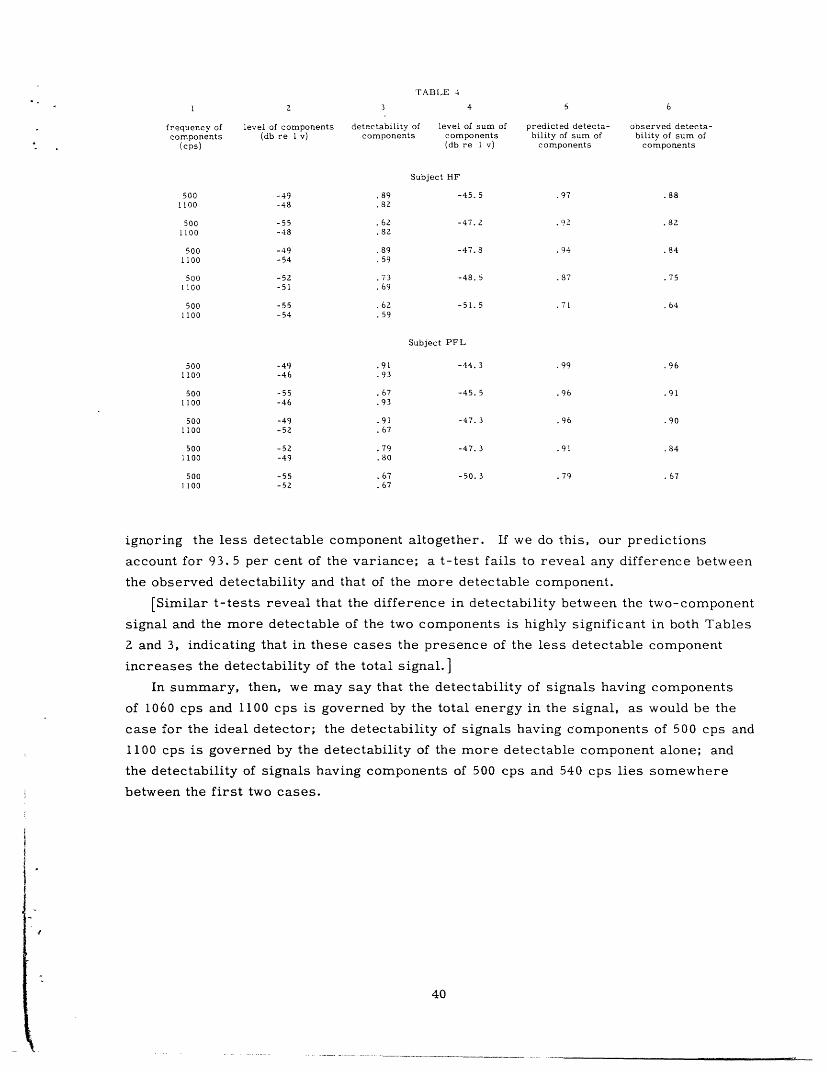
TABLE 4

frequency of level of components detectability of level of sum ofcomponents (db re v) components components

(cps) (db re 1 v)

5

predicted detecta-bility of sum of

components

observed detecta-bility of sum of

components

5001100

5001100

5001100

5001100

5001100

5001100

5001100

5001100

5001100

5001100

-49-48

-55-48

-49-54

-52-51

-55-54

-49-46

-55-46

-49-52

-52-49

-55-52

. 89

.82

. 62

. 82

. 89

. 59

.73.69

.62

.59

.91

.93

.67

.93

.91

.67

.79

.80

.67

.67

Subject HF

-45. 5

-47. 2

-47.8

-48.5

-51.5

Subject PFL

-44. 3

-45. 5

-47. 3

-47. 3

-50. 3

.97

.92

.94

.87

.71

.99

.96

.96

.91

.79

. 88

. 82

. 84

.75

.64

.96

.91

.90

.84

. 67

ignoring the less detectable component altogether. If we do this, our predictions

account for 93.5 per cent of the variance; a t-test fails to reveal any difference between

the observed detectability and that of the more detectable component.

[Similar t-tests reveal that the difference in detectability between the two-component

signal and the more detectable of the two components is highly significant in both Tables

2 and 3, indicating that in these cases the presence of the less detectable component

increases the detectability of the total signal.]

In summary, then, we may say that the detectability of signals having components

of 1060 cps and 1100 cps is governed by the total energy in the signal, as would be the

case for the ideal detector; the detectability of signals having components of 500 cps and

1100 cps is governed by the detectability of the more detectable component alone; and

the detectability of signals having components of 500 cps and 540 cps lies somewhere

between the first two cases.

I

40

~_ I __ - _ 1 _ _

11. EXPERIMENT 2: DISCUSSION

Our discussion of the results of Experiment 1 led us to speculate about the presence

in the auditory system of mechanisms similar in function to bandpass filters. The

passband of the filter was considered to be centered at the frequency of the signal. In

extending this point of view to the present case of multicomponent signals, it is neces-

sary to visualize a number of such filters, the passband of any one of these overlapping,

perhaps, with that of the filter nearest in frequency.

Case 1

Consider first that both components of the signal are close enough in frequency to

fall within the passband of the same filter. More exactly, if the filter characteristics

are as shown in Fig. 5, assume that the components fall within the flat part of the

characteristic. The detectability of the signal will then depend only on the total signal

energy, independently of the number of components, and on the noise power.

Thus to explain the fact that a signal with components at 1060 cps and 1100 cps is as

detectable as a signal having the same energy but only one component at 1100 cps, we

need only assume that 1060 cps and 1100 cps fall within the flat portion of the same

filter characteristic.

Case 2

Next suppose that the two components are far removed in frequency; let us say that

the component of lower frequency, fl, falls in the middle of the passband of some filter

A, while the component of higher frequency, f2 , falls in the middle of the passband of

some filter B. Assume, moreover, that a negligible amount of power from fl is passed

by B, and a negligible amount from f2 by A; A and B are thus "nonoverlapping." If

the same input containing gaussian noise is applied to both filters, the outputs of the two

filters will be statistically independent. If these filters are now incorporated in signal-

detection systems, the decisions of these two systems will also be statistically indepen-

dent.

All detectors considered thus far have been visualized as devices that calculate, on

each trial, a quantity Z, and, in a symmetrical forced-choice situation, make one or

the other of two responses according as Z is positive or negative. (If the detector is

ideal, Z = L(41 ) - L(T 2 ). If the detector is not ideal, Z is a similar quantity having

larger variance, in accordance with the discussion of sec. 9.) In the present case,

however, we are visualizing two (independent) filters, and hence two detectors. Associ-

ate the random variable Z with the first detector and the (independent) variable Z'

with the second. A simple extension of our earlier model would lead us to say that the

decision as to which response is to be made in the two-detector case rests solely on

the signs of Z and Z'. That is to say, whether R1 or R2 is made depends on which of

the four events

41

1_1_ II I _I ___ ____1_11�_ 1_1 __ll�l___ll_--h-i-L� .-._-----._

(Z > , _' > 0) (Z > , Z' < 0)

(Z < 0, Z' > 0) (Z < 0, Z' < 0)

occurs.

Under such circumstances it can be shown (see Appendix I) that the probability of

making the correct decision as to which response to make is no greater than it would

have been had the decision been based on only one of the two filter outputs, provided we

pick the one that gives us the better results. In other words, if responding on the basis

of the sign of Z gives us better results than responding on the basis of the sign of Z',

we can ignore Z' altogether without lowering the probability of making the correct

response.

Thus, on our model, to explain the fact that a signal with components at 500 cps and

1100 cps is only as detectable as the more detectable of the two components, we need

only assume that 500 cps and 1100 cps fall within the passbands of nonoverlapping filters.

Case 3

The third possible case occurs if the two components are not close enough in fre-

quency to fall within the flat portion of the characteristic of one single filter or far

enough apart to fall in nonoverlapping filters. In that case one of the components falls,

it is assumed, in the flat portion of the characteristic of some filter, while the other

falls on the sloping portion of the same characteristic in such a way as to be attenuated

somewhat (but not so much as to give a negligible output). Here we should expect the

detectability to fall somewhere between Case 1 and Case 2.

Thus, to explain the detectability of a signal with components at 500 cps and 540 cps

we need only assume that these frequencies come within the scope of Case 3.

The nature of the difference in detectability between signals having components at

500 cps and 540 cps and those with components at 1060 cps and 1100 cps implies that the

auditory filters in the neighborhood of 1100 cps have wider bandwidths than those in the

neighborhood of 500 cps. By the argument of section 9 this, in turn, implies that detec-

tability at 500 cps is better than at 1100 cps, which was found to be true in Experiment 1.

Acknowledgment

This author wishes to express his thanks to Dr. J C. R. Licklider and

Dr. Bert F. Green, Jr. Without the guidance of the former and the mathematical

assistance of the latter this project could not have been carried out.

42

�-s------ -----�,�I�: .

Appendix A

Guessing-Correction Formula

The traditional guessing-correction formula is sometimes (ref. 1) given as:

P 1- c (A. 1)

where p is the corrected (or true) proportion of perceptions given that a signal was pre-

sented, p' is the observed proportion of responses given that a signal was presented,

and c is the proportion of responses given that a signal was not presented. Putting this

into probability notation, we have

Pr(R S) - Pr(R S)Pr(P I S) = (A. 2)

1 - Pr(RS)

where S = a signal is. presented, R = a response is made, and P = a perception occurs.

This formula purports to yield the probability of a perception from the probabilities

of responses. We can find its underlying assumptions by writing the identity: !I:i

Pr(RIS) - Pr(R P S) l:Pr(PIS) (A.3) i

Pr(R P S)- Pr(R PS)

Clearly, then, if we assume

Pr(R P. S) = Pr(RIS) (A.4)

and

Pr(R P.S)= 1 (A. 5)

we have the desired correction formula (A. 2).

It is unlikely that we shall ever be able to test the truth of these assumptions (A. 4

and A. 5) directly. If we wish to evaluate them, we must do so with respect to a given

model. We would most likely use such a formula as Eq. A. 2, involving the term P,

only if we had in mind a model that asserts that information is transmitted from signals

to responses through the intermediary state P only. Otherwise, it would not pay to

introduce the state P into the model at all; we would rather talk of the transmission of

information from the signal to the response directly. In other words we would pre-

sumably use Eq. A. 2 only if we had in mind a model that implied, among other things, that

Pr(R P S) = Pr(R P S) (A. 6)

Now, if we believe Eq. A. 6 we can make the following deduction. Write the identity

Pr(RIS) -Pr(R P S)Pr(P S) - _(A. 7)

Pr(R I P S) - Pr(R I P S)

43

I

iII ,I �I

Use assumption (A.4) on identity (A. 7) to get

Pr(PIS) =Pr(R P S) - Pr(R P S)

Pr(R P. S) - Pr(R P S)

Now use assumption (A. 6) on (A. 8) to get

Pr(P IS) =Pr(R P S)- Pr(R P S)

Pr(R P. S) - Pr(R P. S) (A. 9)

This last statement (Eq. A. 9) is undoubtedly false, as anyone who has served as

subject in a threshold experiment would testify. We conclude that the guessing-

correction formula is inapplicable.

44

(A. 8)

1 x·~~~~~~~u~~~~um;.a;.n~~~~~~~~~~~ri~~~~~unaaaarc~~~~~~~~~~~%~~~·L~~~~~ L~~~sp~~~~~': I~~~

Appendix B

Calculation of the Criterion, c, for Optimal Behavior

on Tanner and Swets' Model

We wish to find the value of c for which the expected value E(V) of the payoff is

maximal. This value of c will be denoted by cmax.

The expected value of the payoff is

E(Y) = vI Pr(RIS) Pr(S) + v Z Pr(RIS) Pr(S)

+ v3 Pr(RIS) Pr(S) + v4 Pr(RJS) Pr(S)

= (v 1 - v3 ) Pr(RIS) Pr(S) + (v 2 - v4 ) Pr(RIS) Pr(S)

+ v3 Pr(S) + v4 Pr(S)

E(V) (v 4 - v2) Pr(S) v3 Pr(S) + v4 Pr(S)

(v1 - v 3 ) Pr(S) Pr(RIS)- (v - ) Pr(S) Pr(R ( - Pr(S)E(V) (v1 - v3) Pr(S) Fr(R§) + (v 1 - v3 )

Notice that the denominator on the left side is a positive constant and that the last term

on the right is a constant. Hence to require that E(V) be a maximum is to require that

the following expression be a maximum:

y = Pr(R I S) - p Pr(R S) (B. 1)

where

(v4 - v2) Pr(S)

= (v I - v 3) Pr(S)

From Eqs. 2. la and 2. lb we have

Pr(R IS) = N[d'; c, 1]

Pr(RIS) = N[O; c, 1]

So that

y = N[d'; c, 1] - P N[O; c, 1]

1I - N[c; d', 1] - (1 - N[c; 0, 1])

= P N[c; 0, 1] - N[c; d', 1] + 1 -

Differentiating with respect to c, and setting the derivative equal to zero, we obtain

8 = p n[c; 0, 1] - n[c; d', 1] = 0ac

Hence,

45

I I · I I LI -·I I -·1 1111 -- ---- - -- 1 1~~~~~~~~~~~~~~~~~~~~~~~~~~~~~~~~~~~-·WA~~~~~-~~~sn~~~ II ~~~~~ A~~iiiiiiiiiiiiiiii~;

n[c; d', 1]

P n[c; o, 1 exp [cdl d' 2

In = cd' - 2

c = + = cmaxmaxd' 2

46

·L1.r

Appendix C

Maximum Expected Payoff with Symmetrical Payoff Matrices

From Appendix B, Eq. B. 1, we have that the expected payoff is maximized if and

only if the following quantity is also maximized:

Pr(R IS) - B Pr(R IS) (C. 1)

where

(v4 - v2) Pr(S)

= (v 1 - v3 ) Pr(S)

We say that a payoff matrix is symmetrical if vl = v 4 and v2 = v 3. Thus, for a

symmetrical payoff matrix,

= Pr(S)

Pr(S)

Hence, for a symmetrical payoff matrix the quantity (C. 1), and therefore the expected

payoff, is maximized independently of the v i .

47

11PR", PR.WPP.! 1PZ'q L I IPMW P "'q ~ ~ ~ ~ ~ ~ ~ ~ *

Appendix D

Decision Procedure for Ideal Detection in a Two-Category Forced-Choice Situation

In a yes-no situation we deal with a receiver input, T = (X 1, . . .,X2Tw). This

quantity T has one or the other of two densities according as one or the other of two

states obtains. We have called the two states S and S and the corresponding densities

fSN and fN'We define a payoff matrix

S S

R

R

specifying the value of the two responses R and R in case S or S. The fundamental

theorem (section 3) tells us that the ideal detector behaves according to the rule: Make

response R if and only if L(T) > , where

L() fsN() SN) (X1 ... 2 TW)

fN(\t) N(-X1 X2Tw)

and

(v4 - v2) Pr(S)= (v 1 - v3 ) Pr(S)

The forced-choice situation at first glance looks dissimilar. We have two receiver

inputs, 1 and V2,' one for each of two observation-intervals, let us say 0 to T and T

to 2T. One of these receiver inputs has the density fSN and the other the density fN'

but it is not known how the pairing is to be made.

Otherwise, the situations are the same. We again have two possible states, which

are here called S:S and S:S. We say S:S obtains if 1 has density fSN and T 2 has

density fN; we say S:S obtains if 1 has density fN and 2 has density fSN' We again

define a payoff matrix (which differs from the above only trivially in notation):

S:S S:S

R1

R 2

Let us, however, consider the forced-choice situation to have, not two receiver inputs

48

__

xl(t) 0 < t < T

and

x2 (t) T < t < 2T

but a single input x(t) defined by

xl(t)x(t) =

x2(t)

O<t<T

T < t < 2T

This function x(t) can be represented by a set P/' of 4TW random variables:

\' = (X I , 2 -1, 2TW' X2, 1'2, 2 ' 2, 2TW)

The values of x(t) at sampling points in the range 0 to T are represented by the vari-

ables X1 , i; the values in the range T to 2T by the variables X2 i . Now the quantity 4''has one or the other of two densities according as S:S or S:S obtains. Let us call the

two densities fS:S and fS

In this formulation the forced-choice and yes-no situations do not differ at all as far

as the fundamental theorem is concerned. This theorem then tells us that the ideal

detector behaves according to the rule: Make response R 1 if and only if L'(\ ') > , where

fS:fs :s( ' )

f:s('')and

(v 4 - v z ) Pr(S:S)

(v 1 - v 3) Pr(S:S)

Now consider the quantity

fS:S ( A' ) = fS:S(Xi , 1 ' X- -1, 2TW' X2, 1 ' -' X2, 2TW) (D. 1)

This is the likelihood if S:S obtains, i.e., if signal and noise occur during the interval

from 0 to T and noise alone occurs from T to 2T. Hence the first 2TW variables

have the density fSN and the last 2TW variables have the density fN

We now make the assumption that the samples of noise in the two intervals 0 to T

and T to 2T are statistically independent. This would be true if the noise were caused

by random disturbance in an electrical circuit or if it were drawn from a random-noise

generator. On this assumption we then have

fS:S( ' ) = fSN(X, 1' . X1l, 2TW ) fN(X2, 1' 'X2, 2TW )

fSN(T1) fN(I '2) (D. 2)

49

ij

II

iI/

I;j

U ~i:.

By a similar argument we get

fS:s(') = fN('\I 1 ) fSN ( 2 ) (D. 3)

Hence, the likelihood ratio is

=fSN(*I)11 fN('2) L(kV1)

L' (*') = fSN ( 1) fN( 2)= L(2)

fN(q/) fSN( -k2) L(\Y2 )

Thus, if the noise is independent in the two observation-intervals of the forced-choice

trial, the ideal detector behaves according to the Decision Procedure: Make response

R 1 if and only if L(' 1 ) > ,3 L(\ 2 ).

50II- --`----�� n�.-�rr~Y�n"Tr�e rra,--r�ir�C·Ni�� I*·O-�-·i�i7lr-·a��l irr�·�·�-�-··-r�,--ri�lOll�l*nr; -·rc**Cb�iCI·nT;i�TP* -� �Pr---h-·P··a

;N .

Appendix E

Ideal Detection in a Two-Category Forced-Choice Situation with

Uniform Gaussian Noise

The two receiver inputs are assumed to be independent in the sense of Eqs. D. 1, D.2,

and D. 3. It will be convenient to work with the probability of making an incorrect

response. In a two-category forced-choice situation the two conditional probabilities of

an incorrect response are Pr(R I S:S) and Pr(R2 I S:S).

From Appendix D we have, for an ideal detector,

Pr(R1 I S:S) = Pr(L(XVl) > L(\ 2 ) \ 1 E N, I/2 E SN)

Pr(R2 | S:S) = Pr(L(T 1 ) < 3 L(T'2 ) 1 41 E SN, P2 E N)

where \IP E SN (or E N) means that has the density fSN (or fN); hence P 1 E SN,

P2 E N means the same as S:S, and 1 E N, 2 E SN means the same as S:S.

We can put these expressions in the following form (interchanging subscripts through-

out the second equation):

Pr(R 1 I S:S) = Pr( L(P/1 ) > L(I/2 )I 1 E N E SN) (E.Oa)

Pr(Rz I S:S) = Pr(p L(\ 1 )> L( I 2 ) I/1 EN N 2 E SN) (E. Ob)

We can find Pr(R1 I S:S) by computing the probability that (1/p) L( 1 ) is greater than

some number b and that L( I/2) = b, and then integrating over all b:

Pr(R1 I S:S)

Pr( L(P) > b I E N) Pr(L(T) = b I t E SN) (E. la)

0

Likewise we can write

Pr(R2 i S:S) =

Pr(p L(I/) > b \ E N) Pr(L(\) = b I P E SN) (E. lb)

By definition we have

Pr(L(P) > b 1 E N) = FN(b) (E.Za)

Pr(L(T) > b I E SN) = FSN(b) (E. b)

The author is indebted to Dr. Bert F. Green, Jr., for several of the results of thisappendix.

51

bT-FBr

A probability element of Eq. 2.b can be written

Pr(L(\') = b I E SN) = -d FSN(b) (E.3)

The unusual minus sign appears because of the unusual direction of the inequality in

Eq. E. 2b. See Peterson and Birdsall (ref. 15, Part I, p. 27).

Putting Eqs. E. 2a and E. 3 into Eqs. E. la and E. lb we have

Pr(R I S:S)=

Pr S:

FN(Pb) d FSN(b)

FN() )d FSN(b)

Case of the Signal Known Exactly

From Peterson and Birdsall (ref. 15, Part II, p. 10) we have, for the case of the

signal known exactly,

N 1/2FN(b) ( )N 4rE

00

a 1exp [ dyexp - 2E-y dy

N 1/2d FSN(b) = -(4E)

where

Ea = + n b

o

Let

2Eg-

0

g; then a = - + In b

2

1/2 0,0 [ 2FN(b) = (-~/ exp - - dy

\: g 1 Lz Zg

d FSN(b) = -(1/2

exp [- g (a - g) da

Substituting Sb for b in Eq. E. 5a, we have

f0FN(Pb) = 2/

2F yexp i-- dy

L 2g-

where

52

(E. 4a)

(E. 4b)

and

(E. 5a)

(E. 5b)

(E.6)

__ __ ·

I d

exp -.- - d4E N1·

g ga' =-+ In pb =-+ In b + n p

2 2

= a + n

Substituting b/p for b in Eq. E. 5a, we have

F(b)=(2_~g)i/2 oo [ y2]wh FNP)(= gf exp -g dy d

where

g b ga" =- + ln- = - + In b - in

2 P 2

= a - n

We can now write an expression for

Eqs. E.4a, we have

Pr(RI I S:S) = - . ( )/

Pr(R 1 S:S).

co J

I exp -Ja Z g

Putting Eqs. E. 5b and E. 6 into

d} - (t1 exp[ (a[-g) 2-dy~. {~( - exp -- 1daJ ~ \ ~ / [ Z g j

00 00

J- oc Ja '

g exp + (a - g) dy da (E. 9)

Notice that the range of integration in Eq. E. 4a is from 0 to oo, while the range on the

outside integral here is from -oo to oo. The change occurs because in Eq. E.4a the

integration is with respect to b, while here it is with respect to a = E/N o + In b; and

O < b < oo implies -oo a < oo.

We now make the transformation

u=a-y-g

v=y

du dv = dy da

Recalling that a' = a + In , the old range of integration in Eq. E. 9 was

a + n p< y- < oo

_oo a oo

The corresponding new range of integration, in terms of u and v, will be

-o u . - n [ - g

-oo v < aO

so that Eq. E.9 becomes

53

(E. 7)

(E.8)

--�I)---

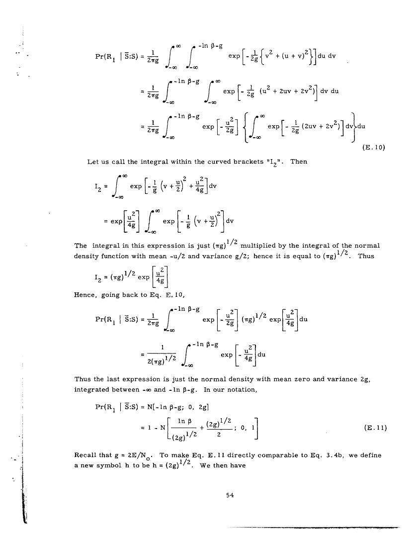
Pr(R1 I S:S) =

-n -g1

Zirgexp - 1 v2 + (u + v)2}] du dv

exp [- 2g (uZ + Zuv + 2v2] dv du

-In P-g1g exp 1uC2gooexp - 2 (2uv + 2v2 ) dv}du

(E. 10)

Let us call the integral within the curved brackets

I2 =

xc

"II "2' Then

exp ( + u)2 + 2dv9~~+- dv4

1/2~~~~ ~1/2The integral in this expression is just (rtg) / 2 multiplied by the integral of the normaldensity function with mean -u/2 and variance g/2; hence it is equal to (g)l / 2 Thus

I 2 = (g)/2 exp g]

Hence, going back to Eq. E. 10,

Pr(R 1 I S:S) 21g = n

x-f exp [- 2g (lTg) exp du

exp [-4jdu

Thus the last expression is just the normal density with

integrated between -oo and -In P-g. In our notation,

mean zero and variance 2g,

Pr(R 1 S:S) = N[-ln P-g; O, 2g]

L(Zg)l/2 2 (E. 11)

Recall that g = 2E/N o . To make Eq. E. 11 directly comparable to Eq. 3.4b, we define

a new symbol h to be h = (2g)/2. We then have

54

o in -g /oo

__ ~

I - In P-g1/

Z(-ffg)

Pr(R1 S:S) = 1- N + 2; 0, I] (E.12)

where h2 = 4E/N o .

The development for Pr(R 2 I S:S) differs from the above only in that Eq. E. 8 is used

instead of Eq. E. 6. The net effect of this change is only to change the sign of n in

Eq. E. 7. This sign is carried throughout. Hence,

Pr(Rz, I S:S) = 1- N[- n +h O, 1]

Or, writing the probability of being correct when S:S occurs, that is, Pr(RI S:S)

1 - Pr(R2 I S:S), we have

Pr(R1 I S:S)= 1 - N IN[lP ] 0(E. 13)h 2

where h2 = 4E/N o .

Case of the Signal Known except for Carrier Phase

This case will be treated only for the special condition that p = 1.

We shall deal with signals of the form

s(t) = f(t) sin[y t + +(t) - P] (E. 14)

where P is a random variable with rectilinear distribution.

For this case Eqs. E. 17-E. 20 hold, as is shown by Peterson and Birdsall in ref-

erence 15. (See their Eqs. 4.19, 4. 22, 4. 25, and 4. 26.)

First we define the quantity a by the following equation.

b = exp o N] 'o((N) ) (E. 15)

where Io(x) is the zero-order modified Bessel function of the first kind; Io(x) is a mono-tonically increasing function having the properties

Io(x) > 1; Io(0) = 1 (E.16)

In terms of these definitions we have

L(P) = exp [N I ) (E. 17)

FN(b) = exp ] (E. 18)

55

d FSN(b) = -exp [- ] a exp Ij ((No) ,' da

FSN(b) = exp E x ex[ 2 ((N ) dxxN N0 2 o N0

(E. 19)

(E. 20)

From Eqs. E. 16 and E. 17 we see that in the present case the likelihood ratio, oddly

enough, is never smaller than bo = exp[-E/No]. Since FSN(b) (Eq. E. 20) is the proba-

bility that the likelihood ratio exceeds b, we have FSN(bo) = 1. From Eqs. E. 15 and

E. 16 we see that when b = bo , a = O. Hence

FSN(bo) = exp x ex dx = SN ~ ~ 2] ) ~0~~~~~~~~~~~~~~~I 0ko/xd(E. 21)

We have thus established the identity

x exp- I 2 x dx = exp

:oo i_~_l0 N(o)/ 0 N '_o

(E. 22)

Let us substitute E/2 for E in this identity; we obtain

x exp x ]I((E) x) dx = exp[ -x~~~ ex %

(E. 23)

Now express the identity in terms of the variable y =

are unchanged by this transformation. We get

0x0 ~ o~,/ ~~~ef y expyi I0 _ 2E)/ dy exp E0 N 2N

0 Ilii";

We write Eq. E.4a for = 1, recalling that in the

b to oo:o

x/2. The limits of integration

(E. 24)

present case the range of b is from

Pr(R1 I S:S) = -

0

Introducing Eqs. E. 18 and

accordingly, we have

FN(b) d FSN(b)

E. 19 into Eq. E. 25 and changing the range of integration

Pr(R1 I S:S) = exp[ E a exp[- a2] I

56

(E.25)

a) da (E. 26)

-- -· �----L-� .�-CR_�_�D--·I··�---u�·n�.�.���n;T·

ZE /?-

The integral in Eq. E. 26 is identical with Eq. E.24. Hence

Pr(R1 S:S) = exp[No 2 exp E[ =ex ] (E. 7)

The parallel development for Pr(R2 I S:S) yields, as might be expected, the same

function:

Pr(R 2 I S:S) = exp - (E.28)

Thus the probability of being correct when the signal occurs in the first observation-

interval is

Pr(R1 i S:S) = 1 -2 exp- (E.29)

57

aA~~~~~~~~~ ~~~~~~ n~~~~~~s~~. . - 1M

Appendix F

Fitting Normal Ogives to the Obtained Psychophysical Data:

A Quick Statistical Test

We have fitted function (8.2) to the data of Experiment 1 by allowing this function to

be displaced to the right or left along the horizontal axis. Thus the fitted curves are

given by

1 exp[- 10(r - a ) /1 0 (F. 1)Z 2

where a is the constant to be determined by the fitting procedure.

As an alternative we can try fitting a normal ogive. This curve, as ordinarily

written, y = N [r; ,, 2-], is asymptotic to y = 0, and thus is not comparable to Eq. F. 1,

which is asymptotic to y = 0. 5. We should like a function that has the properties of the

normal ogive and is also asymptotic to y = 0.5. The desired function is

y = +N [r; , o- ] (F.2)

This function is asymptotic to y = 0.5 and y = 1, and has an inflection point at y = 0. 75

(where r = ).

Function (F. 2) is easily shown to be symmetric about its inflection point, in the

sense that if, for given values of and - , a point (r, y) is on the curve, then the image

(r', y') of this point (reflected through the inflection point of the curve) is also on the

curve; the image being defined by

r' = 2 - r

y' = 2(0. 75) - y

Pictorially we can think of the curve (F. 2) as coming in two sections that are pivot-

ed at the point Pc at which y = 0. 75. Rotating the lower section about Pc by 180 ° super-

imposes it on the upper section.

Function (F. 1), on the other hand is not symmetrical about the point Pc at which

y = 0. 75. If we pivot the lower part of this curve about Pc by 180 ° , we find it falling

below the upper part. The distance between points on the upper part of the curve and

corresponding points on the pivoted lower part is zero when y = 0. 75, and becomes very

small as y assumes values very close to unity; for 0. 90 < y < 0.99, however, this dis-

tance is of the order of 10 per cent of the range of y.

We wish to test the null hypothesis Ho that the data-points fall randomly about a true

underlying ogive (F. 2). To perform the test, each point below the line y = 0. 75 is pro-

jected through Pc to form an image above this line. On Ho each image has an equal

chance of falling above or below its corresponding point on the upper part of the curve.

On the alternative hypothesis H 1 that the true underlying curve is given by the

58

detection-theoretic function (F. 1), an image has greater probability of falling below its

corresponding point.

Our test consists in counting the number g of images which fall below their corre-

sponding points. If this number is greater than could reasonably be expected on the basis

of even chance, we feel justified in rejecting H o .

In practice, three difficulties may arise in performing the test. (a) The location of

Pc must be estimated; if there is doubt concerning the proper value to assume, various

estimates must be made and the test repeated with each estimate. This procedure, of

course, must then be taken into account in the statistical handling of go. (b) If the data-

points are equally spaced along the abscissa, Pc must fall either above or below a data-

point or half-way between the abscissas of two data-points; otherwise the image of a

point would not fall directly either above or below its corresponding point. If Pc cannot

be so located, the test must be performed for each of the nearest appropriate values of

Pc' (c) The data-points may not be equally spaced along the abscissa. In this case

appropriate makeshift repairs may suggest themselves, or the test may be considered

inapplicable.

The test was applied to the four sets of data-points of Experiment 1 (Fig. 3). For-

tunately, none of the difficulties mentioned above manifested itself.

Only points on the upper part of the curve for which 0.90 < y < 0.99 were used in the

test. In all, 17 such points were compared with corresponding images of points from

the lower portion of the curve. All 17 differences were in the direction predicted on H 1 ,

leading to a significant rejection of the null hypothesis.

Changing our estimate of Pc by ± 1 db does not effect the result of the test.

While the test rejects the normal-ogive hypothesis, it does not, of course, prove H 1.

The results of the test are, however, compatible with the latter hypothesis.

59

Appendix G

Bandwidth of the Ideal Filter

As mentioned in section 9, the ideal filter for the detection of sinusoids of known

frequency and amplitude but unknown phase has an impulse response

h(t) =cos[a(T - t)]

0

0<t<T(G. 1)

otherwise

where a is the signal frequency in radians per second, and T is the signal duration. To

simplify matters, let us set a or T so that aT = 2n (n is an integer). The impulse

response is then

h(t) =cos at 0<t<T

0(G. 2)

otherwise

The desired power-gain-versus-frequency characteristic of the filter is the power

spectrum of the impulse response. In performing the Fourier analysis we use the nota-

tion and formulas given by Goldman (6). The Fourier integral is written

h(t) = 1 S(w) cos[wt + L(t)] do

where S2(c), the power spectrum, is given by

h

h(t) sin wt dt

We shall also use the Fourier-integral energy theorem

S2 () d = f h (t) dt

Applying Eq. G. 2 to Eq. G.4, we have

SZ (c ) do = 2 t=T sin 2aT T/2cos 2 atdt =-+ 4a T/22 4a =/

since aT = 2rn.

Applying Eq. G. 2 to Eq. G. 3, we find S (a):

T

h(t) cos at dt= cos 2 at dt = T/2

60

1/I00

(G. 3)

1 / f

(G.4)

Jco

(G. 5)

2

S2(w) = h(t) cos t d +i-o

f" h(t) sin at dt = cos at sin at dt

= - (cos ZaT - 1) = 0

so that S2(a) = TZ/4.

We now apply to the filter input a sinusoidal signal of frequency a and power p0 and

a flat noise of power m ° per radian/second. That part of the output caused by the sig-

nal will have power K p S(a) = 1/4 K po T 2 , where K is a proportionality constant,

and that part of the output caused by the noise will have an over-all power of

Km S2( ) d = 1/2 K m T

where the equality holds by virtue of Eq. G. 5. The output signal-to-noise ratio will

therefore be, in power units,

po T

Zirmo

Consider applying the same signal and noise to a filter having rectangular gain-

versus-frequency characteristic over a band Aw wide (see section 9). The output caused

by the signal will have power C p,0 and the output caused by the noise will have power

C mo0 Aw. The output signal-to-noise ratio will therefore be po/(mo A). Letting Aw

= Zr/T, we have a filter whose output signal-to-noise ratio is equal to that of the filter

originally considered. We say then that the equivalent rectangular bandwidth of the

original filter is Ac = 2/T, or, in cycles per second, Af = 1/T.

61

__�1___ __I____

Appendix H

The Sum of Two Sinusoids Expressed as a Frequency- and Amplitude-Modulated

Sinusoidal Carrier

Certain results obtained by Peterson and Birdsall (15) were used in the derivation

of Eq. 8.2. These results apply to situations in which the signal can be expressed as

s(t) = f(t) sin[at + (t) - P] (H. 1)

where P is a random variable with rectilinear distribution.

The signals used in Experiment 2 can be written as

s 1 (t) = A1 sin(wlt + P 1 ) + A2 sin(w2 t + P 2 ) (H.2)

In order for Eq. 8.2 to be applicable to Experiment 2, it is necessary to show that

Eq. H. 2 can be put in the form of Eq. H. 1.

Let

11 = lt + P 1

12 = 2t + P2

13 = 12 - 11

Equation H. 2 can then be written

sl(t) = A 1 sin 11 + A 2 sin(ll + 13)

= A sin 11 + A2 (sin 11 cos 13 + cos 11 sin 13)

s 1 (t) = (A 1 + A 2 cos 13) sin 11 + (A2 sin 13) cos 11 (H. 3)

Let

A2 sin 13

Al + A 2 cos 13

and

-14 = tan u

We then have

cos -l1/(u2 + 1)1/2

sin + = u/(u2 + 1)1/2

We can then write

62

- ~ ~ ~ ~ ll

sin 11 u cos 1sin(11 + )(= uZ 1)/. 4)

(u + 1) u + 1)1/2

and, replacing several of the u in Eq. H. 4 by the definition of u, we have

(A 1 + A2 cos 13) sin 11 + (A 2 sin 13) cos 11

sin(11 +) =

(Al +A 2 cos 13) (u + 1)/ Z

sl(t)

(Al + A cos 13) (u 2 + 1)1/2

replacing 11 by its definition, letting the denominator in the above equation be fl(t), and

writing 1 = q4(t ) , we have, finally,

sl(t) = fl(t) sin[wlt + l1(t) + Pl ]

which is in the desired form of Eq. H. 1. The amplitude modulation is thus given by

fl(t) = (A 1 + Az cos 13) (u2 + 1)1/2

= (A + A 1 + 2 A 1A2 cos[(w 2 - w)t + (P - P)])

and the frequency modulation is given by

A z sin[(w 2 - l)t + (P 2 - P1) ]

4)1(t) = tanA1 + A2 cOS[(w 2 - °l)t + (P2 - P1 ) ]

For sl(t) to fulfill the requirements of randomness associated with Eq. H. 1 it is

necessary (a) that P 1 be a random variable having rectilinear distribution, and (b)

that P2 - P 1 be constant, since f(t) and +(t) are required to be ordinary (nonrandom)

functions. Condition (a) is very likely approximated in Experiment 2 (as already dis-

cussed in connection with Experiment 1). Condition (b) is not met.

It is highly likely, however, that, from the point of view of the auditory mechanism,

it is irrelevant whether requirement (b) is met or not. A change in the difference

between phases is equivalent to a change in the time at which the observation-interval

begins, i.e., equivalent to a change in the location of the observation-interval along an

infinite signal waveform. So long as the duration of the observation-interval is large

compared to a period of the waveform (as is the case in Experiment 2), such changes

cannot matter to the ear. Had the condition of constant phase-difference been met, our

data and our comparisons between ideal-detector behavior and actual behavior would

have remained unchanged.

63

I FW~- -- --- I-

I

LI1

, 1

Appendix I

Detection with Two Independent Detectors in a Symmetrical

Two-Category Forced-Choice Situation

Ideal Detection

To show: Detection with two independent detectors is no better than detection with

only the better one of the two.

The symmetrical two-category forced-choice procedure is characterized by [3 = 1

and Pr(S:S) = Pr(S:S). We wish to maximize the quantity Pr(R1 I S:S) + Pr(R z I S:S).

From Appendix D we have that the ideal decision procedure is to make response R

if and only if L(' 1 ) > L(T 2 ). Let us define

= L(T 1 ) - L(T 2 )

The procedure is then to make response R1 if and only is Z > 0.

Now consider a second ideal detector operating simultaneously; this second detector

calculates a quantity Z', which is independent of Z in the sense that

Pr(Z > 0, Z' > 0 S:S) = Pr(Z > 0 S:S) Pr(Z' > 0 S:S)

Pr(Z > 0, Z' > 0 S:S) = Pr(Z > 0 S:S) Pr(Z' > 0 S:S)

For ideal detectors we have, obviously, (for either Z or Z'),

Pr(Z > 0 I S:S) > Pr(Z > 0 I S:S)

(I. la)

(I. lb)

(I. 2)

A decision procedure for two detectors consists of a plan that assigns one of the two

responses to each of the four possibilities

(Z < 0, Z' > 0)

(Z < 0, Z' < 0)

There are, in all, sixteen possible

represented abstractly by the matrix

decision procedures. These procedures may be

Z> Z<

Z' > A A2

Z' < A A 4

To obtain any particular procedure we replace each Ai by either R 1 or R 2 .

64

(Z > 0, Z' > 0)

( > , z' < o)

- ------

a. The Two Detectors Agree. It is easy to decide which response to make if the two

detectors agree: A is R1 and A4 is R 2 . That is to say, if the two detectors agree,

make the response upon which they agree. This is shown as follows.

We wish to maximize the quantity Pr(R1 I S:S) + Pr(R2 S:S). This quantity may be

written

Pr(Z > 0, Z' > 0 U1) + Pr(Z > O, Z' > U2 )

+ Pr(Z > 0, Z' < U3) + Pr(Z< 0, Z' < O 0 U4) (I. 3)

where Ui is S:S or S:S according as Ai is R1 or R 2 . We maximize (I. 3) by making each

term as large as possible. If we let A 1 be R 1 then the first term of (I. 3)- the only term

affected- is

(I. 4)Pr(Z > 0, Z' > 0 I S:S) = Pr(Z > 0 S:S) Pr(Z' > 0 S:S)

If we let A 1 be R2, the first term of Eq. 1.3 is

Pr(Z > 0, Z' > 0 S:S) = Pr(Z > 0 S:S) Pr(Z' > 0 I S:S) (I. 5)

Referring to (I. 2) we see that (I.4) > (I. 5). Thus we want to let A 1 be R 1. By a similar

argument we show that we want to let A4 be R 2 .

We are therefore left with only four decision procedures to investigate:

Z>0 Z<0

R 1 RI

R1 R 2

Z' >0

Z' <0

Procedure 1

Z>0 Z<0O

Z>0 Z<O

R 1 R 2

R2 R 2

Procedure 2

Z>0 Z<0

Z' >O

Z' <0

Procedure 3 Procedure 4

b. The Remaining Four Procedures. It is easy to show that the ideal detector has

the same probability of making the correct response in case S:S as in case S:S. (See

Eq. E.0, Appendix E, letting = 1.) Thus (for either Z or Z')

65

Z' >0

Z' <0

Z' >0

Z' < 0O

R 1 R 2

R 1 R z

R 1 R 1

R2 R2

- III I I ·~~~~·-~~- e a IZIILIRI~~~~~1~ I~~C --1I1P~~~ ~~P~;F?~~i~~E-`=·`-~~Pli~~iE---~~~-?iT3~~;·a~,I

Pr(Z > 0 S:S) = Pr(Z < 0 S:S)

Assume first that the Z-detector is better than the Z'-detector, that is, assume that

Pr(Z > 0 S:S) > Pr(Z' > 0 S:S) (I. 7)

By writing out expression (I. 3) explicitly for each of the four decision procedures, and

then applying (I. 2), (I. 6), and (I. 7), it is easy to convince oneself that (I. 3) is maximal

for procedure 3. But procedure 3 is equivalent to paying attention only to the Z-detector,

as is evident from the matrix. By (I. 7) the Z-detector is the better of the two detectors.

Assume next that the Z'-detector is the better of the two. That is, instead of (I. 7),

assume

Pr(Z > 0 S:S) < Pr(Z' > 0 S:S) (I. 8)

In this case by writing out (I. 3) explicitly for the four procedures, one can convince

himself that procedure 4 is optimal. But this procedure is equivalent to paying attention

only to the Z'-detector, which is, by (I. 8), the better of the two.

Lastly, assume that the two detectors are equally good, that is, instead of (I. 7) or

(I. 8), assume

Pr(_Z > 0 S:S) = Pr(Z' > 0 S:S) (I. 9)

In this case we can convince ourselves, by writing out (I. 3) explicitly for all four cases,

that all four decision procedures are equally good. Thus we can arbitrarily choose to

consider only one of the two detectors. This completes the proof.

Nonideal Detection

When dealing with nonideal detection, we assume once again that there exist quan-

tities Z and Z' that are similar to those quantities in the case of ideal detection, at

least to the extent that Eq. I. 2 holds. In that case the proof given above holds through

section a; that is we need to investigate only four decision procedures. On the other

hand the part of the proof in section b may no longer hold, through failure of (I. 6) to

hold.

We can however make an empirical investigation. To calculate the expected detect-

ability on each of the four decision procedures we need to know

Pr(Z > 0 S:S) and Pr(Z < 0 S:S) (I.9)

Pr(Z' > 0 S:S) and Pr(Z' < 0 S:S) (I.10)

But by our model these probabilities are equal to

Pr(R1 I S:S) and Pr(R 2 S:S)

which have been measured in our experiment. Thus we may take the observed

66

_1_11__1_11111111111��I�BB�PB��

(I. 6)

Pr(R1 I S:S) and Pr(R2 I S:S) for the case of a 500-cps signal, letting these be the prob-

abilities in (I. 9). Then take the observed Pr(R1 I S:S) and Pr(R I S:S) for the case of

an 1100-cps signal, letting these be the probabilities in (I. 10). On the basis of these

values we may then calculate for each of the four decision procedures what the observed

detectability for the combination of these two tones would have been had detection been

performed by two independent detectors, one listening to each tone.

These calculations were carried out five times, once for each of the five conditions

of Table 4 for subject HF. In none of these five cases was the predicted combined

detectability on any of the four decision procedures higher than the detectability of the

more highly detectable component. Thus, in our experiment, the theorem holds for

nonideal detection.

67

Phil~~ ~ II I11 II _11 ~n'-·-- - - ·- ·-- ----- -rr~rr

Appendix J

Some Background Notes on Detection Theory

The theory of detection is generally recognized to be a special case of the statistical

theory of hypothesis-testing. And, as there are two general approaches to the theory of

hypothesis-testing, we find two corresponding approaches to the theory of detection.

The older approach to hypothesis-testing consists in the calculation by means of

Bayes's theorem of the a posteriori probability of the hypothesis under test, as in the

following example.

Example. Consider the following two hypotheses S and S about a given coin (we

assume that these are the only admissible hypotheses).

S: The probability of the coin landing heads is 1/11.

S: The probability of the coin landing heads is 10/11.

Suppose moreover, that for one reason or another, we are able to assign specific

a priori probabilities to the two hypotheses. Thus, suppose that

Pr(S) = Pr(S) = 1/2

We decide to evaluate our hypotheses on the basis of K, the number of heads that

occur in two independent tosses of the coin. First, let us write the probability dis-

tribution of K on each of the two hypotheses. If S obtains, we have

( = kS) = k! (2-k) (1/11) (10/11)2 -Pr(K = kS) k! (2-k)!

If S obtains, we have

Pr(K= kS= k k! (Z-k)! (10/11) (1/11) -

Now write Bayes' s theorem,

Pr(K = k S)Pr(S)Pr(S K = k)=

Pr(K = k S) Pr(S) + Pr(K = k S) Pr(S)

Introducing our a priori probabilities and probability distributions into Bayes' s

theorem, we have

Pr(S I K = k) -1 + (10) -

Thus, for instance, if we observe that K = 2, that is, if we obtain two heads, we

find that the a posteriori probability of the hypothesis S is

Pr(S K = 2) = 1/101

Proponents of the Bayes' s theorem approach argue that obtaining a low value for

68

���� ----I�I-II-�I�1�---�------L1-·ll��----_� �-·�i?·ii-�i�Cg=T�=CIc��i�i�----�Br_� ·

I

the a posteriori probability of a hypothesis is evidence against that hypothesis. Thus,

in our example, we would be said to have found evidence that hypothesis S is (probably)

false.

The application of this theory to the problem of detection is immediate: The hypoth-

esis to be tested is that the "input to the detector" (see section 3) contains the

signal in addition to the noise; due to the presence of the random noise, this input is a

random variable whose distribution on the hypotheses may be calculated once the char-

acteristics of the signal and of the noise are specified; the a priori probability of the

hypothesis is assumed known.

Detection theory along the lines just discussed has been developed primarily by

Woodward and Davies (22, 23, 24;, 25). In support of their approach these authors show

that a detector that calculates the a posteriori probability extracts all the possible

relevant information from its input; if we are required to specify how certain we are

that a signal was present, we cannot give a better answer than the a posteriori prob-

ability.

In a series of joint papers beginning in 1928 Neyman and Pearson proposed an

alternative approach to hypothesis-testing. Their theory - which forms the basis for a

good portion of modern statistics - and their objections to the earlier Bayes' s theorem

approach are contained in the following quotation (14):

Now what is the precise meaning of the words "an efficient test of a hypothesis ?"There may be several meanings. For example, we may consider some specifiedhypothesis , as that concerning the group of stars, and look for a method which weshould hope to tell us, with regard to a particular group of stars, whether theyform a system, or are grouped "by chance," their mutual distances apart beingenormous and their relative movements unrelated.

If this were what is required of an "an efficient test," we should agree withBertrand in his pessimistic view [that no statistical test could give reliable results].For however small be the probability that a particular grouping of a number of starsis due to "chance," does this in itself provide any evidence of another "cause" forthis grouping but "chance?" "Comment definir, d' ailleurs, la singularite dont onjuge le hasard incapable?" Indeed, if x is a continuous variable - as for exampleis the angular distance between two stars - then any value of x is a singularity ofrelative probability equal to zero. We are inclined to think that as far as a partic-ular hypothesis is concerned, no test based upon the theory of probability can byitself provide any valuable evidence of the truth or falsehood of that hypothesis.

But we may look at the purpose of tests from another viewpoint. Withouthoping to know whether each separate hypothesis is true or false, we may searchfor rules to govern our behaviour with regard to them, in following which weinsure that, in the long run of experience, we shall not be too often wrong. Here,for example, would be such a "rule of behaviour": to decide whether a hypothesis,H, of a given type be rejected or not, calculate a specified character, x, of theobserved facts; if x > x reject H, if x < x accept H. Such a rule tells us nothingas to whether in a particular case H is true when x < x or false when x > x .But it may often be proved that if we behave according to such a rule, then in thelong run we shall reject H when it is true not more, say, than once in a hundredtimes, and in addition we may have evidence that we shall reject H sufficientlyoften when it is false.

The decision-procedure approach of Neyman and Pearson is illustrated in the

following example.

69

__ _ ��U�

Example. Let the situation be the same as in the preceding example, and consider

the following decision procedure: Reject the hypothesis S if and only if two heads come

up in the two tosses of the coin.

We now calculate the probability of being in error if we follow this procedure. If S

is true, the probability of rejecting S is

Pr(K = 2S) = (1/11) = 0.008

If S is false (i.e., if S holds), the probability of accepting S is

Pr(K 2 S) = 1 - Pr(K = 2 ) = 1 - (10/11)2 = 0. 17

These probabilities of error may, of course, be reduced by devising different decision

procedures based on a larger number of throws of the coin.

Notice, incidentally, that if we are satisfied with calculating these conditional prob-

abilities of error, we do not need to know the a priori probabilities associated with the

hypotheses. Only if we wish to calculate the absolute (unconditional) probability of

error need the a priori probabilities enter the picture.

Neyman and Pearson suggest the following criterion for an optimal decision procedure

to test hypothesis H: Pick the procedure so that (a) the probability of rejecting H when it

is true is a small given number, and (b) the probability of accepting H when it is false is

simultaneously minimized. They show that the calculation of such optimal procedures

rests primarily on the calculation of the likelihood ratio (see section 3) of the random

variable in question. Their theory thus leads to the modern "likelihood ratio tests."

The Neyman-Pearson theory was applied to signal-detection by Lawson and

Uhlenbeck in 1950 (ref. 10, chap. 7). These authors, however, do not follow Neyman

and Pearson' s suggested criterion for the optimal decision procedure. Instead, they

use as criterion the minimization of the absolute probability of error. As already men-

tioned, this requires the specification of the a priori probability of the relevant hypoth-

eses. Despite this change of criterion, Lawson and Uhlenbeck' s theory remains - to

quote the authors themselves - "practically identical with the Neyman-Pearson theory"

(ref. 10, p. 168).

Both approaches to detection theory are reviewed in the comprehensive monograph

by Peterson and Birdsall (15). These authors suggest a somewhat more general crite-

rion of optimal procedures than that used by Lawson and Uhlenbeck: As their criterion

they use the maximization of the "payoff values" associated with the two kinds of correct

and the two kinds of incorrect decisions that may be made in a detection situation (see

sections 2, and 3). This again, however, does not affect the basic theory materially.

In addition to exhibiting extensive proofs of many of the major results in detection theory,

Peterson and Birdsall solve the decision-procedure model explicitly for a wide variety

of interesting specific situations.

Among other workers who have contributed to detection theory may be mentioned

Kaplan and Fall (9), Marcum (12), Middleton (13), and Reich and Swerling (17).

70

M*raa�llrarmraara�ll�8�sn*rrs*msnrrrr� ill

NOTATION FOR PROBABILITIES

"Pr(A)" designates the probability of the occurrence of the event A. "Pr(AIB)" desig-

nates the probability of the occurrence of the event A, given that the event B occurs.

Superscribed bars always indicate complementary events. Thus, for any events A

and B,

Pr(A) + Pr(A) = 1

Pr(AIB) + Pr(AIB) = 1

Distribution Functions and Densities

If Y is a random variable and if

Pr(Y < y) = F(y)

then F(y) is called the distribution function (or, briefly, the distribution) of Y.

If F(y) has a derivative

d F(y)

dy = f(y)

then f(y) is called the probability density of Y. Thus

f f(x) dx = Pr(Y < y) = F(y)

71

"P WA- i -i;- - ._-' .- X-- -_----._ -----~~l=~r--- ----- ----------- ·- ·- --- 1 ··1

NOTATION AND FORMULAS FOR THE NORMAL DISTRIBUTION

The normal, or gaussian, distribution function, i.e.,

1 C -1

( /is represented by exp 2

is represented by Nix; [, ].

( - )2 dt

Thus, to say that the random variable Y is normally

distributed with mean E(Y) and variance Var(Y) is to say that

Pr(Y < y) = N[y; E(Y), Var(Y)]

The normal density is written: n[x; [±, - 2].

Thus

(z)/2 exp 1-a-(2T) Li= n[x; , C2] 1

The reader is assumed to be familiar with the following identities:

Nix; , 1 = - 2i; o, = N[x - ; o, 1]

N[x; O, 2 - 1 - N[-x; , r 2]

72

REFERENCES

1. Blackwell, H. R. Psychophysical Thresholds, Engineering Research InstituteBulletin No. 36, University of Michigan, 1953.

2. Davies, I. L. On determining the presence of signals in noise, Proc. Instn. Elec.Engrs. (London) 99, Part III, 45-51 (1952).

3. Fletcher, H. The mechanism of hearing as revealed through experiments on themasking effect of thermal noise, Proc. Nat. Acad. Sci. 24, 265-274 (1938).

4. Fletcher, H. Auditory patterns, Revs. Modern Phys. 12, 47-65 (1940).

5. Goldman, S. Information Theory (Prentice-Hall, Inc., New York, 1953).

6. Goldman, S. Transformation Calculus and Electrical Transients (Prentice-Hall,Inc., New York, 1949).

7. Guilford, J. P. Psychometric Methods (McGraw-Hill Book Company, Inc.,New York, 1936).

8. Hawkins, J. E. and Stevens, S. S. The masking of pure tones and of speech bywhite noise, J. Acoust. Soc. Am. 22, 6-13 (1950).

9. Kaplan, S. M. and Fall, R. W. The statistical properties of noise applied toradar range performance, Proc. IRE 39, 56 (1951).

10. Lawson, J. L. and Uhlenbeck, G. E. Threshold Signals (McGraw-Hill BookCompany, Inc., New York, 1950).

11. Licklider, J. C. R. Basic correlates of the auditory stimulus, in Handbook ofExperimental Psychology, S. S. Stevens, Ed. (John Wiley and Sons, Inc.,New York, 1951).

12. Marcum, J. I. A Statistical theory of target detection by pulsed radar: mathe-matical appendix, Report R-113, Rand Corporation, Santa Monica, California, 1948.

13. Middleton, D. Statistical criteria for the detection of pulsed carriers in noise,J. Appl. Phys. 24, 371 (1953).

14. Neyman, J. and Pearson, E. S. On the problem of the most efficient tests ofstatistical hypotheses, Trans. Roy. Soc. (London) A231, 289-337 (1933).

15. Peterson, W. W. and Birdsall, T. G. The theory of signal detectability, TechnicalReport 13, Electronic Defense Group, University of Michigan, 1953.

16. Peterson, W. W., Birdsall, T. G., and Fox, W. W. The theory of signal detect-ability, Trans. IRE, Vol. PGIT-4, 171-212 (Sept. 1954).

17. Reich, E. and Swerling, P. The detection of a sine wave in Gaussian noise,J. Appl. Phys. 24, 289 (1953).

18. Schafer, T. H., Gales, R. S., Shewmaker, C. A., and Thompson, P. O. Thefrequency selectivity of the ear as determined by masking experiments, J. Acoust.Soc. Am. 22, 490-496 (1950).

19. Tanner, W. P. and Swets, J. A. A new theory of visual detection, TechnicalReport 18, Electronic Defense Group, University of Michigan, 1953.

20. Tanner, W. P. Psychophysical application of the theory of signal detectability,Electronic Defense Group, University of Michigan, February 1954.

21. Tanner, W. P. and Swets, J. A. A decision-making theory of visual detection,Psychol. Rev. 61, 401-409 (1954).

22. Woodward, P. M. and Davies, I. L. Information theory and inverse probabilityin telecommunications, Proc. Instn. Elec. Engrs. (London) 99, Part III, 37 (1952).

23. Woodward, P. M. Information theory and the design of radar receivers, Proc. IRE39, 1521 (1951).

24. Woodward, P. M. Probability and Information Theory, with Applications toRadar (McGraw-Hill Book Company, Inc., New York, 1953).

25. Woodward, P. M. and Davies, I. L. A theory of radar information, Phil. Mag.41, 1521 (1950).

73

~Fa~, , ~L , ~ - ·-~~33~gAp$?~T~-s-iaa~~ile · P"-~-~~UC-.- I~·~Lmm now - irr._-·--S__P·-ii