1

Detection of Sclerotinia Rot Disease on Celery Using Hyperspectral Data and Partial Least Squares Regression

Jing-feng Huang1, 2 and Armando Apan2

1 Institute of Agricultural Remote Sensing & Information Application, Huajiachi Campus

Zhejiang University, Hangzhou, 310029, Zhejiang, China Phone: +86 571 8697-1830 Email: hjf@zju.edu.cn

2 Faculty of Engineering and Surveying & Australian Centre for Sustainable Catchments

University of Southern Queensland, Toowoomba 4350 QLD Australia Phone: +61 7 4631-1386 Fax: +61 7 4631-2526 Email: apana@usq.edu.au

Abstract

There is a need to detect and assess the incidence of Sclerotinia rot disease in celery

(Apium graveolens). In this study, we examined the potential of hyperspectral sensing to

detect the symptoms of this disease in celery crop. Using a portable spectrometer, sample

measurements of diseased and healthy leaves were collected from celery leaves in the

field. Both raw and transformed spectral data were used in the development of Partial

Least Squares regression models. The cross-validated results showed that the incidence of

disease on celery could be predicted using the raw spectra and the first and second

derivative data, with prediction errors ranging from 11.08 to 13.62%. The visible and

near-infrared wavelengths (400-1300nm) produced similar detection ability with that of

the full range wavelengths (400-2500nm).

2

INTRODUCTION

Detecting plant health condition is of primary importance to agricultural field

management (Bryant and Moran, 1999). In crop protection, the ability to delineate

infected areas in agricultural fields will improve the efficiency of prophylactic methods,

which might consist of targeted agrochemical applications and implementing crop

rotations at a regional scale using non-susceptible crops. Traditionally, disease damage

assessment in crop populations has been done by using visual approach, i.e. relying upon

visual observation to assess the incidence of disease in the field. However, this method is

time-consuming, labor–intensive, and costly for disease monitoring in large-scale farming

(Lucas, 1998, p. 54). Therefore, there is a need to develop different approaches that can

enhance or supplement traditional techniques.

The use of remote sensing for crop disease assessment started many decades ago. In the

late 1920s, aerial photography was used in detecting cotton root rot disease (Taubenhaus

et. al., 1929). In the early 1980s, Toler, et al., (1981) used aerial colour infrared

photography to detect root rot of cotton and wheat stem rust. Most of these studies

involved the use of airborne cameras that record the reflected electromagnetic energy on

analogue films covering broad spectral bands. Reflectance data was found to be capable

of detecting pathogen-induced biophysical changes in the plant leaf and canopy. Since

then, however, remote sensing technology has advanced significantly. Modern sensors

have superior spatial, spectral and radiometric resolutions, thereby offering enhanced

capabilities to detect and map disease symptoms.

The presence of disease in crops can alter its reflectance properties. In the visible (VIS)

wavelengths (~ 400nm to 700nm), the reflectance of healthy vegetation is relatively low

3

due to strong absorption by pigments. If affected by disease the reduction in pigment

activity causes an increase in VIS reflectance. Vigier et al. (2004) found that the red

wavelengths contributed the most in the detection of sclerotinia stem rot in soybeans. On

the other hand, the reflectance of healthy vegetation in the near-infrared (NIR) region

(~700nm to 1300nm) is significantly high. With a disease that damaged the leaves (e.g.

cell collapse), the reflectance in the NIR region is expected to be lower. For stress in

tomatoes induced by a late blight disease, it was found that the NIR region was much

more valuable than the VIS range to detect disease (Zhang, et al., 2002). Furthermore, in

the shortwave infrared (SWIR) range (~1300nm to 2500nm), the spectral properties of

vegetation are dominated by water absorption bands. Less water on leaves and canopies

will increase reflectance in this region. Apan et al. (2004) noted the key role of the SWIR

bands in the discrimination of healthy and diseased (orange rust) sugarcane crops.

Hyperspectral sensing, a technique that utilises sensors operating in hundreds of narrow

contiguous spectral bands, offers potential to improve the assessment of crop diseases.

Data acquired from such sensors may allow the capture of specific plant attributes (e.g.

foliar biochemical contents) previously not detectable with broadband sensors. Although

some laboratory work has been done in characterising the spectral properties for tomato,

potato, beans and barley diseases (Blazquez and Edwards, 1983; Lorenzen and Jensen,

1989; Malthus and Madeira, 1993), no study was found in the literature that focuses on

Sclerotinia rot on celery. Furthermore, very little is known about the comparative

detection ability of using the VISNIR regions as against the use of full-range (VIS, NIR,

and SWIR) wavelengths in the context of disease detection.

Sclerotinia rot, caused by the fungus Sclerotinia sclerotiorum, develops on mature

4

celery. In addition, the fungus causes damping-off in infected seedbeds. The pink rot

phase is characterised by rapid development of basal crown and petiole rot. Plants appear

to suddenly wilt and collapse in the field. This rotted area is watery, pinkish, and in moist

conditions may become covered with a conspicuous white mold that sometimes contains

hard black sclerotia (pea-sized fungal reproductive structures). The sclerotia persist for

many years in soil. The disease develops best under moist conditions in cool to moderate

temperatures.

Therefore, the aim of the study was to examine the potential of hyperspectral sensing to

detect the symptoms of Sclerotinia rot disease in celery crop. The specific objectives

were: (a) to compare the spectral response obtained from the healthy and

Sclerotinia-infected celery crop; b) to determine if the visible and near-infrared

wavelengths (400-1300nm) will have a comparatively similar detection ability with that

of the full range wavelengths (400-2500nm); and (c) to determine the best spectral bands

relevant to Sclerotinia rot detection in celery crop.

MATERIALS AND METHODS

Study site and data collection

The study was conducted at Westview Gardens, Wyreema (approx. 27.61°S, 151.88°E,

and 564m above sea level), located in the Darling Downs region of Queensland, Australia.

The site is part of a commercial vegetable production company that grows lettuce, celery

and cauliflower crops. The area was selected to incorporate a range of celery grown in the

area at that time, which was affected by Sclerotinia. The identification of the disease was

done in consultation with the farm agronomist. On 4th February 2005, we collected 30

infected samples and 41 non-infected samples. In this study, the samples collected were

5

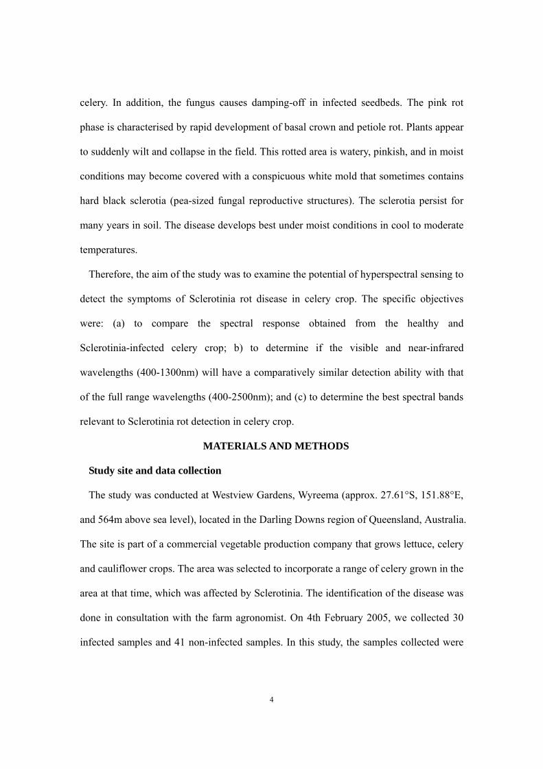
in the severity levels of 3 to 4, based on our defined 1–5 scale, where 1 has the lowest

severity rating and 5 with the highest severity rating. Severity rating 1 corresponded to

those leaves with light yellow-green colour in less than 50% of the total leaf area, while

rating 5 leaves appeared brown for greater than 80% of the leaf area (Figure 1b).

a b Figure 1. A photograph showing (a) healthy and (b) infected celery leaves

An Analytical Spectral Devices (ASD) field spectrometer was used to collect

reflectance measurements from celery leaves in the field. This device is a portable battery

powered spectrometer with a fiber optic cable for light collection and a notebook

computer for data logging (Analytical Spectral Devices, 2002). This device records

reflected sunlight between 350 nm and 2500 nm wavelengths at 1 nm intervals. The

instrument set-up involved switching on the ASD and notebook computer, optimising the

ASD with existing sunlight levels and measuring a “white reference” reading using a

spectralon panel. The white reference panel reflects nearly 100% of the light and the

subsequent readings from the crop canopies are divided by this reference reading to give

a reflectance value at each wavelength of between 0 and 1 (0-100%).

The canopy reflectance data were collected by pointing the fiber optic cable over the

6

celery leaf, and pressing a key on the notebook computer to record the spectrum. Each

sample corresponded to a field of view of about 1.5 cm diameter or 4.7 sq. cm area. The

computer screen displays a plot of the current spectrum in real time. For each sample, ten

spectra were internally averaged by the ASD spectrometer. All data were collected on

clear sunny days between 10 am and 2pm local time. To account for the changing sun

angle and atmospheric conditions with time of day, the white reference reading was taken

every 10 minutes. The field data collection was non-invasive, with no removal of any

plants/leaves and no plant material was in contact with the instrument.

Data Transformation and Partial Least-Squares Regression

The key data pre-processing steps and Partial Least-Squares (PLS) Regression were

illustrated in Figure 2. Graphical plots of the spectra were firstly examined to check for

potential erroneous samples, as well as to initially explore the nature and magnitude of

the difference between sample measurements. Then, a series of “cleaning” operations

were implemented using a spreadsheet program: a) exclusion of very short wavelengths

(341-399nm) and strong water vapour absorption bands (1356-1480nm; 1791-2021nm;

2396nm and beyond), and b) exclusion of obvious outliers, by visual observation, that

showed uncharacteristic reflectance response compared with other samples. After five

sample outliers were excluded, the measurements were thus reduced to a data array of 66

samples x 1,982 bands.

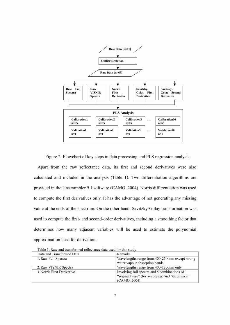
7

Raw Data (n=71)

Outlier Dectetion

Raw Data (n=66)

PLS Analysis

Calibration3n=65

Validation3n=1

Calibration2n=65

Validation2n=1

Calibration1n=65

Validation1n=1

Calibration66n=65

Validation66n=1

Raw Full Spectra

Raw VISNIR Spectra

Norris First Derivative

Savitzky-Golay First Derivative

Savitzky-Golay Second Derivative

…

…

Figure 2. Flowchart of key steps in data processing and PLS regression analysis

Apart from the raw reflectance data, its first and second derivatives were also

calculated and included in the analysis (Table 1). Two differentiation algorithms are

provided in the Unscrambler 9.1 software (CAMO, 2004). Norris differentiation was used

to compute the first derivatives only. It has the advantage of not generating any missing

value at the ends of the spectrum. On the other hand, Savitzky-Golay transformation was

used to compute the first- and second-order derivatives, including a smoothing factor that

determines how many adjacent variables will be used to estimate the polynomial

approximation used for derivation.

Table 1. Raw and transformed reflectance data used for this study Data and Transformed Data Remarks 1. Raw Full Spectra Wavelengths range from 400-2500nm except strong

water vapour absorption bands 2. Raw VISNIR Spectra Wavelengths range from 400-1300nm only 3. Norris First Derivative Involving full spectra and 5 combinations of

“segment size” (for averaging) and “difference” (CAMO, 2004)

8

4. Savitzky-Golay First Derivative Involving full spectra and 21 combinations of variable (data point) taken into account on the left and right side of the value to be averaged, and the order of the polynomial (CAMO, 2004)

5. Savitzky-Golay Second Derivative (same as item 4 above) Partial least squares (PLS) regression, a type of eigenvector analysis, was used to relate

hyperspectral data response to celery Sclerotinia rot data. PLS regression methods reduce

full-spectrum data into a smaller set of independent latent variables or principal

components (PCs). As a result, full-spectrum wavelength loadings for significant PLS

factors, from which regression coefficients for each wavelength are derived, describe the

spectral variation most relevant to the modeling of variation in the data (Kramer, 1998).

Unlike the classical multiple regression technique, PLS performs particularly well when

the various predictor X-variables have high correlation and that the number of predictor

variables is greater than the number of samples.

Several implementations of the PLS algorithm have been reported. For a calibration

model between an independent variable C and spectral data matrix A, each of these

methods produces a model of the form

111 ×××× +×= nkknn ebAC where n is the number of observations (i.e., spectra), k is the number of variables (i.e.,

spectral resolution elements), b is a vector of PLS regression coefficients, and e is the

model residual vector. The PLS calculation employed here mean-centered the

independent variable and spectral variables, thereby producing a model with no intercept

term. The computed means of the calibration data were saved and subsequently used in

applying the model for prediction (Zhang and Small, 2002).

The accuracy of developed equations was evaluated using the residual mean square

error of prediction (RMSEP) statistic, based on an iterative calibration–validation

9

algorithm (leave-one-out cross validation). Each variable and its associated spectra were

iteratively excluded, and a prediction of the sample value was made based on an equation

developed using the remaining samples. The process is repeated until every sample has

been left out once, and then all prediction residuals are combined to compute the

validation equation statistics and RMSEP. The RMSEP is effectively equivalent to the

standard error of prediction (SEP) for an independent dataset (Kramer, 1998).

RESULTS

Analysis of Raw Spectra

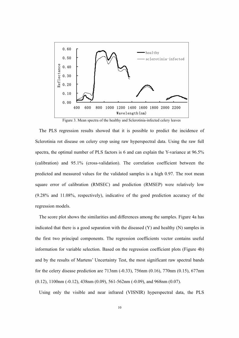
As expected, the reflectance values of healthy celery leaves in the visible region

(400–700 nm) are lower than those of Sclerotinia-infected samples (Figure 3). This is

because infected plants often contain lower chlorophyll levels that lead to a lower

absorbance in the visible region (Blazquez and Edwards, 1983). The reverse is true for

the near infrared region: diseased samples have lower reflectance than healthy samples.

In the short wave infrared region, disease-affected leaves have relatively lower

reflectance values than unaffected sites from 1525nm to 1790nm. But from 1481 nm to

1524 nm and from 2022nm to 2395nm, leaves with Sclerotinia rot have higher

reflectance values than healthy celery.

10

0.00

0.10

0.20

0.30

0.40

0.50

0.60

400 600 800 1000 1200 1400 1600 1800 2000 2200

Wavelength(nm)

Reflectance

healthy

sclerotinia-infected

Figure 3. Mean spectra of the healthy and Sclerotinia-infected celery leaves

The PLS regression results showed that it is possible to predict the incidence of

Sclerotinia rot disease on celery crop using raw hyperspectral data. Using the raw full

spectra, the optimal number of PLS factors is 6 and can explain the Y-variance at 96.5%

(calibration) and 95.1% (cross-validation). The correlation coefficient between the

predicted and measured values for the validated samples is a high 0.97. The root mean

square error of calibration (RMSEC) and prediction (RMSEP) were relatively low

(9.28% and 11.08%, respectively), indicative of the good prediction accuracy of the

regression models.

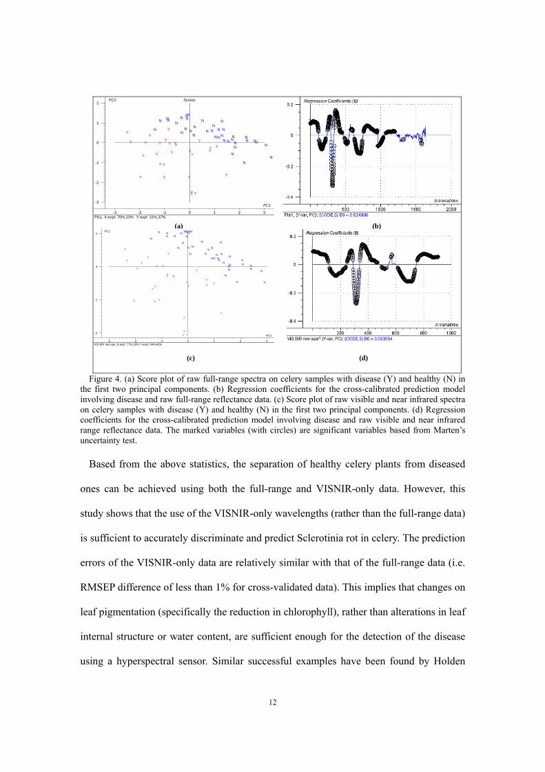
The score plot shows the similarities and differences among the samples. Figure 4a has

indicated that there is a good separation with the diseased (Y) and healthy (N) samples in

the first two principal components. The regression coefficients vector contains useful

information for variable selection. Based on the regression coefficient plots (Figure 4b)

and by the results of Martens’ Uncertainty Test, the most significant raw spectral bands

for the celery disease prediction are 713nm (-0.33), 756nm (0.16), 770nm (0.15), 677nm

(0.12), 1100nm (-0.12), 438nm (0.09), 561-562nm (-0.09), and 968nm (0.07).

Using only the visible and near infrared (VISNIR) hyperspectral data, the PLS

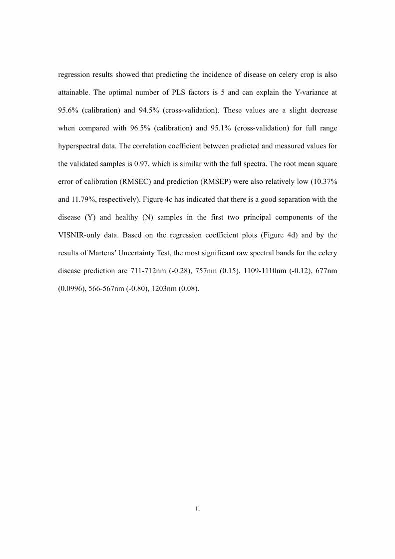
11

regression results showed that predicting the incidence of disease on celery crop is also

attainable. The optimal number of PLS factors is 5 and can explain the Y-variance at

95.6% (calibration) and 94.5% (cross-validation). These values are a slight decrease

when compared with 96.5% (calibration) and 95.1% (cross-validation) for full range

hyperspectral data. The correlation coefficient between predicted and measured values for

the validated samples is 0.97, which is similar with the full spectra. The root mean square

error of calibration (RMSEC) and prediction (RMSEP) were also relatively low (10.37%

and 11.79%, respectively). Figure 4c has indicated that there is a good separation with the

disease (Y) and healthy (N) samples in the first two principal components of the

VISNIR-only data. Based on the regression coefficient plots (Figure 4d) and by the

results of Martens’ Uncertainty Test, the most significant raw spectral bands for the celery

disease prediction are 711-712nm (-0.28), 757nm (0.15), 1109-1110nm (-0.12), 677nm

(0.0996), 566-567nm (-0.80), 1203nm (0.08).

12

-3

-2

-1

0

1

2

-3 -2 -1 0 1 2 3 Pls1, X-expl: 70%,23% Y-expl: 31%,37%

Y

YYY Y

Y

Y

YY

Y

Y

Y

Y

Y

Y

YY

Y

Y

Y

Y

Y

YY

Y

Y

YY

N

N

N

NNN

N

N

N

N

N

NN

N

N NN

N

N

NN

N

N

N NN

N

N

N

NNN

NN

N

N

N

N

PC1

PC2 Scores

(a) (b)

-2

-1

0

1

-3 -2 -1 0 1 2 3 VIS BIR raw spe…, X-expl: 77%,19% Y-expl: 34%,42%

Y

YY

Y

YY

Y

Y

Y

Y

Y

Y

Y

Y

Y

YY

Y

Y

Y

Y

Y

Y

Y

Y

Y

Y

Y

N

NN

NN

N

NN

N

N

N

N

N

N

N N

N N

N

NN

N

N

N

N

N

N

N

N

NN

N

N

N

N

N

N

N

PC1

PC2 Scores

(c) (d)

Figure 4. (a) Score plot of raw full-range spectra on celery samples with disease (Y) and healthy (N) in

the first two principal components. (b) Regression coefficients for the cross-calibrated prediction model involving disease and raw full-range reflectance data. (c) Score plot of raw visible and near infrared spectra on celery samples with disease (Y) and healthy (N) in the first two principal components. (d) Regression coefficients for the cross-calibrated prediction model involving disease and raw visible and near infrared range reflectance data. The marked variables (with circles) are significant variables based from Marten’s uncertainty test.

Based from the above statistics, the separation of healthy celery plants from diseased

ones can be achieved using both the full-range and VISNIR-only data. However, this

study shows that the use of the VISNIR-only wavelengths (rather than the full-range data)

is sufficient to accurately discriminate and predict Sclerotinia rot in celery. The prediction

errors of the VISNIR-only data are relatively similar with that of the full-range data (i.e.

RMSEP difference of less than 1% for cross-validated data). This implies that changes on

leaf pigmentation (specifically the reduction in chlorophyll), rather than alterations in leaf

internal structure or water content, are sufficient enough for the detection of the disease

using a hyperspectral sensor. Similar successful examples have been found by Holden

13

and LeDrew (1998) who used spectral properties to discriminate healthy and unhealthy

corals. They concluded that the greatest changes in reflectance were detected in the

visible (chlorophyll absorption) and near infrared regions of the spectrum, which agrees

with what we observed in our results. Therefore, due to equipment costs and portability

considerations, it suggests that the VISNIR-only spectroradiometers may be preferred

over the full-range version for Sclerotinia rot detection in celery.

Analysis of First Derivative Data Partial Least Square Analysis of Norris First Derivative. Table 2 presents the PLS

regression results of celery disease and Norris first derivative values. The explained Y

variances vary from 95.48% to 95.89% (calibration) and from 93.57% to 94.27%

(cross-validation), which is a slight decrease compared with the raw spectra. The optimal

number of PLS factors was 3 for all combinations of averaging size and difference. For

the calibrated samples, the correlation coefficients between predicted and measured

values vary from 0.9771 to 0.9792. The correlation coefficients between predicted and

measured values for validated samples vary from 0.9665 to 0.97. The root mean square

errors (RMSEC) are from 10.01% to 10.51% for calibration samples. The root mean

square errors of prediction (RMSEP) were from 12.01% to 12.73%. These values suggest

that the use of Norris first derivative, did not significantly improve the disease prediction

accuracy (when compared with the use of raw data), even if various combinations of

averaging size and difference values are used.

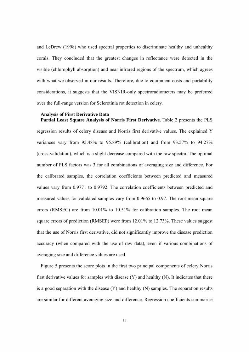
Figure 5 presents the score plots in the first two principal components of celery Norris

first derivative values for samples with disease (Y) and healthy (N). It indicates that there

is a good separation with the disease (Y) and healthy (N) samples. The separation results

are similar for different averaging size and difference. Regression coefficients summarise

14

the relationship between all predictors and a given response. Table 3 shows the most

significant Norris first derivative spectral bands for the celery disease prediction. They

are 728-730nm, 691nm, 1131-1133nm, 956-957nm, 663nm, 509nm. These values

generally correspond to the regions identified by the analysis of raw spectra

Table 2. PLS regression results of celery disease and Norris first derivative values Calibration Cross-Validation

(leave-one-out) Data (n=66)

Optimal of PLS factors R* RMSEC**

value % of Y

Variance Explained

R* RMSEP*** value

% of Y Variance Explained

3-2§ 3 0.9792 0.1001 95.89 0.9665 0.1273 93.57 5-4 3 0.9792 0.1003 95.88 0.9696 0.1211 94.18 7-6 3 0.9781 0.1028 95.67 0.9699 0.1203 94.25 9-8 3 0.9775 0.1043 95.54 0.9700 0.1202 94.26

11-10 3 0.9771 0.1051 95.48 0.9700 0.1201 94.27 R*─correlation between predicted and measured values. RMSEC**─root mean square error of calibration.

RMSEP***─root mean square error of prediction. 3-2§─3 averaging size and the difference between the variables for the differentiation is 2.

Table 3. The most significant Norris first derivative spectral bands for the celery disease prediction

Data Transformation

Label Rank 1st Rank 2nd Rank 3rd Rank 4th Rank 5th Rank 6th

λ (nm) 730 691 1133 957 663 509 3-2§ RC* 6.47 -6.05 2.60 2.46 1.66 -1.41

λ (nm) 729-730 691 1131 956 663 509 5-4 RC 6.60 -6.54 3.11 2.52 1.77 -1.49

λ (nm) 729 691 1132 956 663 509 7-6 RC 6.72 -6.71 3.41 2.53 1.79 -1.55

λ (nm) 728 691 1132 956 663 509 9-8 RC 6.84 -6.71 3.58 2.49 1.79 -1.59

λ (nm) 728 691 1132 956 663 509 11-10 RC 6.98 -6.65 3.75 2.53 1.77 -1.64

RC*—regression coefficient. 3-2§—3 averaging size and the difference between the variables for the differentiation is 2.

15

-0.03

-0.02

-0.01

0

0.01

0.02

0.03

-0.04 -0.02 0 0.02 0.04 PLS1 norris de? X-expl: 54%,19% Y-expl: 54%,34%

Y

YY

Y

YYY

Y

Y

Y

YY

Y

Y

Y

Y

Y

Y

Y

YY

Y

Y

Y

Y

Y

Y

Y

N

N

N

N

N

N

NN

N

N

N

N

N

N

NN

NN

N

N

N

N

N

N

N

N

N

N

N

N

NN

N

N

N

N

N

N

PC1

PC2 Scores

Figure 5. Score plot of celery Norris first derivative values samples with disease

(Y) and healthy (N), in the first two principal components. The averaging size is 3, and the difference between the variables for the differentiation is 2.

Partial Least Square Analysis of Savitzky-Golay First Derivative. Table 4 shows

selected results for the PLS regression analysis of Savitzky-Golay first derivative data.

When the order of the polynomial is 2, the Y-variances explained by the transformed

spectral data vary from 95.4% to 97.5% (calibration) and from 93.9% to 94.4%

(cross-validation). The optimal number of PLS factors was 3. The correlation coefficients

between predicted and measured values for the calibrated samples vary from 0.9765 to

0.9874 and from 0.9683 to 0.9705 for the validated samples. The root mean square error

of calibration (RMSEC) and prediction (RMSEP) were relatively low, i.e. 7.44% to

10.65% for the calibration samples and 11.92% to 14.53% for the cross-validation

samples, respectively. The results are basically similar when the polynomial used was 3.

This suggests that the influence of the number of variables to be averaged and the order

of the polynomial on the PLS regression results of celery disease and Savitzky-Golay

first derivative values is not significant.

The score plots (Figure 6) also indicate that there are good separations with the disease

(Y) and healthy (N) samples in the first two principal components using the first

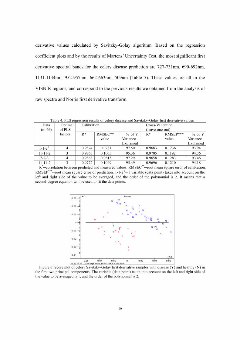
16

derivative values calculated by Savitzky-Golay algorithm. Based on the regression

coefficient plots and by the results of Martens’ Uncertainty Test, the most significant first

derivative spectral bands for the celery disease prediction are 727-731nm, 690-692nm,

1131-1134nm, 952-957nm, 662-663nm, 509nm (Table 5). These values are all in the

VISNIR regions, and correspond to the previous results we obtained from the analysis of

raw spectra and Norris first derivative transform.

Table 4. PLS regression results of celery disease and Savitzky-Golay first derivative values Calibration Cross-Validation

(leave-one-out) Data

(n=66) Optimal

of PLS factors R* RMSEC**

value % of Y

Variance Explained

R* RMSEP*** value

% of Y Variance Explained

1-1-2§ 4 0.9874 0.0781 97.50 0.9683 0.1236 93.94 11-11-2 3 0.9765 0.1065 95.36 0.9705 0.1192 94.36 2-2-3 4 0.9863 0.0813 97.29 0.9658 0.1283 93.46

11-11-2 3 0.9772 0.1049 95.49 0.9696 0.1210 94.18 R*─correlation between predicted and measured values. RMSEC**─root mean square error of calibration.

RMSEP***─root mean square error of prediction. 1-1-2§─1 variable (data point) takes into account on the left and right side of the value to be averaged, and the order of the polynomial is 2. It means that a second-degree equation will be used to fit the data points.

-0.04

-0.03

-0.02

-0.01

0

0.01

0.02

0.03

-0.06 -0.04 -0.02 0 0.02 0.04 0.06 PLS1 S G 1st? X-expl: 60%,14% Y-expl: 42%,45%

Y

YY

YY

YY

Y

Y

Y

YY

Y

Y

Y

Y

Y

Y

Y

Y Y

Y

Y

Y

Y

Y

Y

Y

N

N

N

N

NN

N

N

N

N

N

N

N

N

N N

NN

N

NN

N

N

N

N

N

N

N

N

N

N N

NN

N

N

N

N

PC1

PC2 Scores

Figure 6. Score plot of celery Savitzky-Golay first derivative samples with disease (Y) and healthy (N) in

the first two principal components. The variable (data point) taken into account on the left and right side of the value to be averaged is 1, and the order of the polynomial is 2.

17

Table 5. The most significant (rank 1-4 out of 21 combinations) Savitzky-Golay first derivative spectral

bands for the celery disease prediction Data

Transformation Label Rank

1st Rank 2nd Rank 3rd Rank 4th Rank 5th Rank 6th

λ(nm) 731 692 1133 957 662-663 509 1-1-2§ RC 7.16 -6.44 2.80 3.03 1.47 -1.48 λ(nm) 727 692 1134 953 663 509 11-11-2 RC 7.27 -6.84 4.11 2.74 1.82 -1.77 λ(nm) 731 691 1133 957 663 509 2-2-3 RC 7.05 -6.29 2.54 2.96 1.50 -1.46 λ(nm) 728 691 1131 955 663 509 11-11-3 RC 6.67 -6.95 3.47 2.39 1.85 -1.56

RC*—regression coefficient. 1-1-2§—1 variable (data point) takes into account on the left and right side

of the value to be averaged, and the order of the polynomial is 2. It means that a second-degree equation will be used to fit the data points.

Analysis of Savitzky-Golay Second Derivative Data

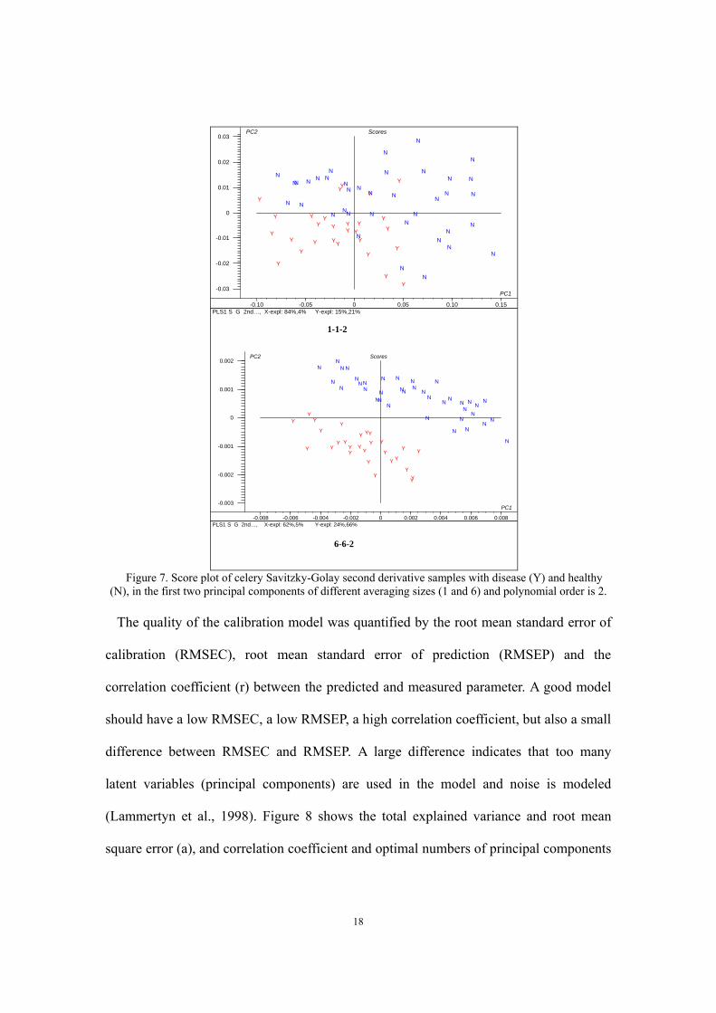
Using the second derivative values calculated by Savitzky-Golay algorithm, the results

indicate that it is difficult to separate the disease from healthy samples when the

averaging size is less than or equal to 4. When the averaging size is more than or equal to

5, the separation results are better. Figure 7 shows the score plots for the

Savitzky-Golay second derivative samples with disease (Y) and healthy (N) for two

different averaging sizes (1 vs. 6), in the first two principal components.

18

-0.003

-0.002

-0.001

0

0.001

0.002

-0.008 -0.006 -0.004 -0.002 0 0.002 0.004 0.006 0.008 PLS1 S G 2nd…, X-expl: 62%,5% Y-expl: 24%,66%

Y

Y

YY

YY

YY

Y

Y

YY

Y

Y

Y

Y Y

Y

Y

Y Y

Y

Y

Y

Y

Y

YY

N

N

N

N

N

N

N

N

N

N

N

N

N

N

N

N

NN

N

N

N

N

N

N

NN

N

NN N

N

N

N N

NN

N

N

PC1

PC2 Scores

-0.03

-0.02

-0.01

0

0.01

0.02

0.03

-0.10 -0.05 0 0.05 0.10 0.15 PLS1 S G 2nd…, X-expl: 84%,4% Y-expl: 15%,21%

Y

Y

YY

Y

Y

Y

Y

Y

Y

Y

Y

Y

YY

Y

Y Y

Y

Y

Y

Y

Y

Y

Y

Y

YY

N

N

N

N

NNN

N N

N

N

NN

NN

N

N N

N

N

N

N

N

N NN N

N

N

N

N

N

N

N

N

N

N

N

PC1

PC2 Scores

1-1-2

6-6-2

Figure 7. Score plot of celery Savitzky-Golay second derivative samples with disease (Y) and healthy

(N), in the first two principal components of different averaging sizes (1 and 6) and polynomial order is 2. The quality of the calibration model was quantified by the root mean standard error of

calibration (RMSEC), root mean standard error of prediction (RMSEP) and the

correlation coefficient (r) between the predicted and measured parameter. A good model

should have a low RMSEC, a low RMSEP, a high correlation coefficient, but also a small

difference between RMSEC and RMSEP. A large difference indicates that too many

latent variables (principal components) are used in the model and noise is modeled

(Lammertyn et al., 1998). Figure 8 shows the total explained variance and root mean

square error (a), and correlation coefficient and optimal numbers of principal components

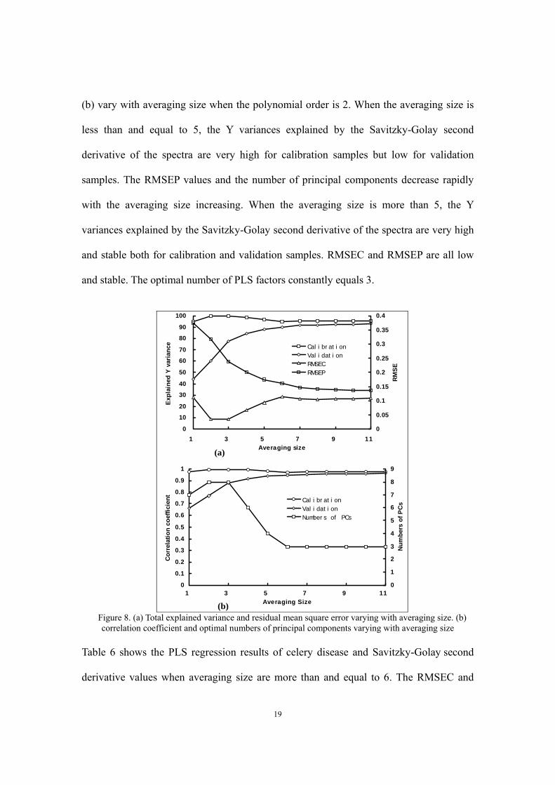
19

(b) vary with averaging size when the polynomial order is 2. When the averaging size is

less than and equal to 5, the Y variances explained by the Savitzky-Golay second

derivative of the spectra are very high for calibration samples but low for validation

samples. The RMSEP values and the number of principal components decrease rapidly

with the averaging size increasing. When the averaging size is more than 5, the Y

variances explained by the Savitzky-Golay second derivative of the spectra are very high

and stable both for calibration and validation samples. RMSEC and RMSEP are all low

and stable. The optimal number of PLS factors constantly equals 3.

0

10

20

30

40

50

60

70

80

90

100

1 3 5 7 9 11Averaging size

Expl

aine

d Y

var

ianc

e

0

0.05

0.1

0.15

0.2

0.25

0.3

0.35

0.4

RM

SE

Cal i br at i onVal i dat i onRMSECRMSEP

0

0.1

0.2

0.3

0.4

0.5

0.6

0.7

0.8

0.9

1

1 3 5 7 9 11Averaging Size

Cor

rela

tion

coef

ficie

nt

0

1

2

3

4

5

6

7

8

9

Num

bers

of P

Cs

Cal i br at i onVal i dat i onNumber s of PCs

(a)

(b) Figure 8. (a) Total explained variance and residual mean square error varying with averaging size. (b) correlation coefficient and optimal numbers of principal components varying with averaging size

Table 6 shows the PLS regression results of celery disease and Savitzky-Golay second

derivative values when averaging size are more than and equal to 6. The RMSEC and

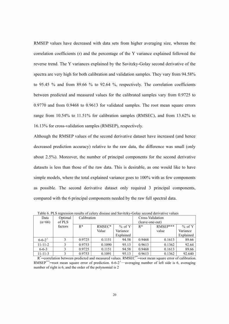
20

RMSEP values have decreased with data sets from higher averaging size, whereas the

correlation coefficients (r) and the percentage of the Y variance explained followed the

reverse trend. The Y variances explained by the Savitzky-Golay second derivative of the

spectra are very high for both calibration and validation samples. They vary from 94.58%

to 95.45 % and from 89.66 % to 92.64 %, respectively. The correlation coefficients

between predicted and measured values for the calibrated samples vary from 0.9725 to

0.9770 and from 0.9468 to 0.9613 for validated samples. The root mean square errors

range from 10.54% to 11.51% for calibration samples (RMSEC), and from 13.62% to

16.13% for cross-validation samples (RMSEP), respectively.

Although the RMSEP values of the second derivative dataset have increased (and hence

decreased prediction accuracy) relative to the raw data, the difference was small (only

about 2.5%). Moreover, the number of principal components for the second derivative

datasets is less than those of the raw data. This is desirable, as one would like to have

simple models, where the total explained variance goes to 100% with as few components

as possible. The second derivative dataset only required 3 principal components,

compared with the 6 principal components needed by the raw full spectral data.

Table 6. PLS regression results of celery disease and Savitzky-Golay second derivative values

Calibration Cross-Validation (leave-one-out)

Data (n=66)

Optimal of PLS factors R* RMSEC*

Value % of Y

Variance Explained

R* RMSEP*** value

% of Y Variance Explained

6-6-2§ 3 0.9725 0.1151 94.58 0.9468 0.1613 89.66 11-11-2 3 0.9753 0.1090 95.13 0.9613 0.1362 92.64 6-6-3 3 0.9725 0.1151 94.58 0.9468 0.1613 89.66

11-11-3 3 0.9753 0.1091 95.13 0.9613 0.1362 92.640 R*─correlation between predicted and measured values. RMSEC**─root mean square error of calibration.

RMSEP***─root mean square error of prediction. 6-6-2§—averaging number of left side is 6, averaging number of right is 6, and the order of the polynomial is 2

21

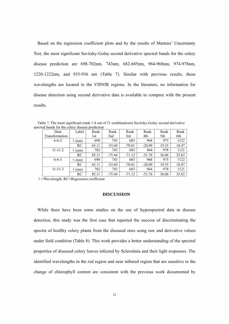
Based on the regression coefficient plots and by the results of Martens’ Uncertainty

Test, the most significant Savitzky-Golay second derivative spectral bands for the celery

disease prediction are 698-702nm, 743nm, 682-685nm, 964-968nm, 974-978nm,

1220-1222nm, and 935-936 nm (Table 7). Similar with previous results, these

wavelengths are located in the VISNIR regions. In the literature, no information for

disease detection using second derivative data is available to compare with the present

results.

Table 7. The most significant (rank 1-4 out of 21 combinations) Savitzky-Golay second derivative

spectral bands for the celery disease prediction Data

Transformation Label Rank

1st Rank 2nd

Rank 3rd

Rank 4th

Rank 5th

Rank 6th

λ(nm) 698 743 683 968 975 1122 6-6-2 RC 65.11 -53.69 -70.01 -20.09 19.35 18.47

λ(nm) 702 743 683 964 978 1121 11-11-2 RC 85.11 -75.44 -71.12 -51.76 36.06 35.63

λ(nm) 698 743 683 968 975 1122 6-6-3 RC 65.11 -53.69 -70.01 -20.09 19.35 18.47

λ(nm) 702 743 683 964 978 1121 11-11-3 RC 85.11 -75.44 -71.12 -51.76 36.06 35.63

λ─Wavelength, RC─Regression coefficient

DISCUSSION

While there have been some studies on the use of hyperspectral data in disease

detection, this study was the first case that reported the success of discriminating the

spectra of healthy celery plants from the diseased ones using raw and derivative values

under field condition (Table 8). This work provides a better understanding of the spectral

properties of diseased celery leaves infected by Sclerotinia and their light responses. The

identified wavelengths in the red region and near infrared region that are sensitive to the

change of chlorophyll content are consistent with the previous work documented by

22

Gitelson and Merzlyak (1997). The infected plants often contain lower chlorophyll levels

that lead to a low photosynthesis rate. The changes on these pigments are often indicators

of plant stress, which can be used to monitor the conditions of crop growth and site

characteristics.

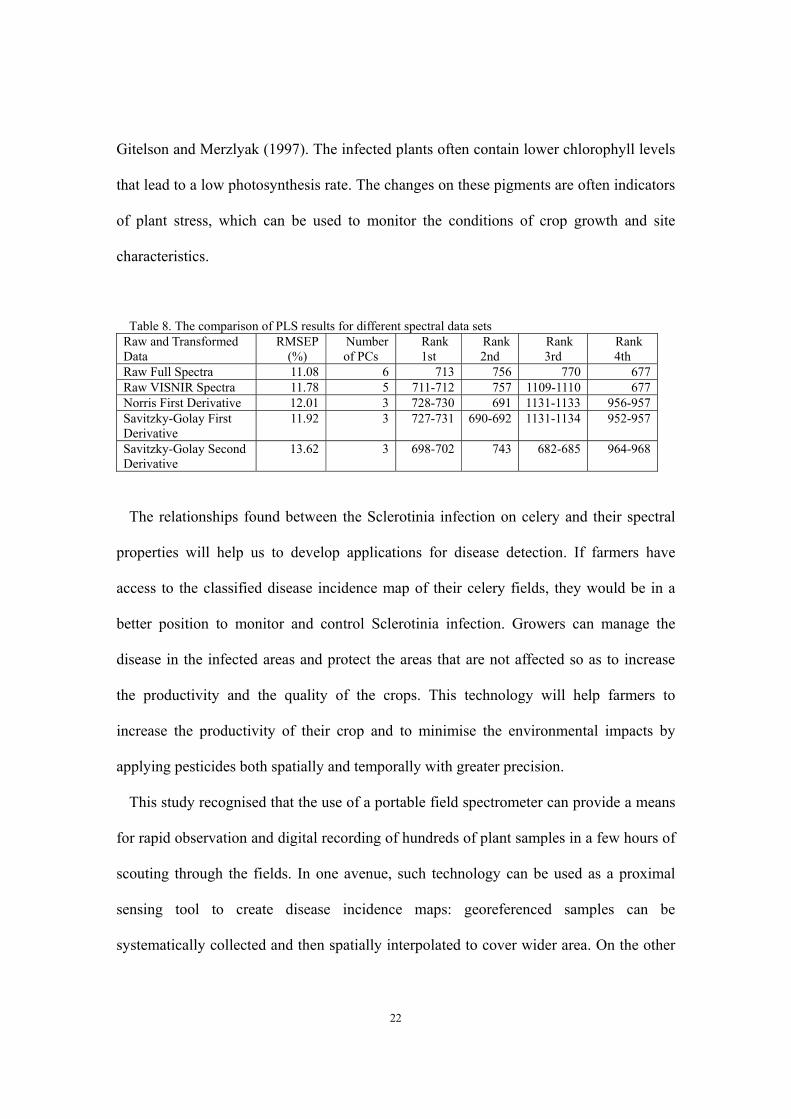
Table 8. The comparison of PLS results for different spectral data sets

Raw and Transformed Data

RMSEP (%)

Number of PCs

Rank 1st

Rank 2nd

Rank 3rd

Rank 4th

Raw Full Spectra 11.08 6 713 756 770 677 Raw VISNIR Spectra 11.78 5 711-712 757 1109-1110 677 Norris First Derivative 12.01 3 728-730 691 1131-1133 956-957 Savitzky-Golay First Derivative

11.92 3 727-731 690-692 1131-1134 952-957

Savitzky-Golay Second Derivative

13.62 3 698-702 743 682-685 964-968

The relationships found between the Sclerotinia infection on celery and their spectral

properties will help us to develop applications for disease detection. If farmers have

access to the classified disease incidence map of their celery fields, they would be in a

better position to monitor and control Sclerotinia infection. Growers can manage the

disease in the infected areas and protect the areas that are not affected so as to increase

the productivity and the quality of the crops. This technology will help farmers to

increase the productivity of their crop and to minimise the environmental impacts by

applying pesticides both spatially and temporally with greater precision.

This study recognised that the use of a portable field spectrometer can provide a means

for rapid observation and digital recording of hundreds of plant samples in a few hours of

scouting through the fields. In one avenue, such technology can be used as a proximal

sensing tool to create disease incidence maps: georeferenced samples can be

systematically collected and then spatially interpolated to cover wider area. On the other

23

hand, ground based hyperspectral sensing will continue to be the test bed for scientific

studies that could underpin future spaceborne or airborne hyperspectral image analysis

systems. In any case, the use of hyperspectral sensing is expected to grow for crop

disease management in the coming years.

However, to best utilise such information, it is necessary to combine it with other data.

The need for a synthesis of remote sensing, ground truthing, spatial and statistical

analysis techniques is readily apparent and is made manifest through the adoption of

Geographic Information System (GIS). These systems and methodologies represent an

essential tool for the enhancement of traditional disease management techniques.

CONCLUSIONS

This study demonstrated that it is possible to detect the effects of Sclerotinia rot disease

in celery crops using hyperspectral measurements. Cross-validated PLS regression

models produced low prediction errors, confirming the usefulness of hyperspectral

reflectance data in detecting the disease in celery. Since the visible and near-infrared

(VISNIR) wavelengths produced similar detection ability with that of the full range

wavelengths, VISNIR-only spectroradiometers may be preferred for Sclerotinia rot

detection in celery due to equipment costs and portability considerations.

The results indicate that raw spectra and the first and second derivative data are

effective for differentiating Sclerotinia-infected from non-infected celery crop. The

models using raw hyperspectral data produced the highest correlation coefficients

between the predicted and measured values, and the lowest prediction errors (RMSEPs).

The most significant raw spectral bands for the celery disease prediction are the red, near

infrared, and blue wavelengths. The first derivatives using the Norris and Savitzky-Golay

24

algorithms produced fairly similar results, with the averaging size produced little

influence on the separability of the disease and healthy samples. However, for the second

derivative data, the averaging size has a significant influence on the results: it is difficult

to separate the disease from healthy samples when the averaging size is less than 5. More

work is needed to test other analytical techniques, for example artificial neural network

method, to further substantiate the results obtained in this study.

ACKNOWLEDGMENTS

The data used in this project was acquired from a research funded by the Rural Industries

Research and Development Corporation (RIRDC), involving Bisun Datt (CSIRO),

Armando Apan (USQ) and Rob Kelly (DPI&F). Tek Maraseni (USQ) provided valuable

help during the fieldwork, while John Duff (DPI&F at Gatton) assisted the team in

contacting the growers. The data was collected from Westview Gardens, Wyreema, with

the support of Lester Hamblin and Andrew Millers.

REFERENCES

Apan, A., Held, A., Phinn, S., and Markley, J. (2004) Detecting sugarcane ‘orange

rust’ disease using EO-1 Hyperion hyperspectral imagery. International Journal of

Remote Sensing, Vol. 25, no.2, pp.489–498.

Analytical Spectral Devices, (2002) Spectroradiometer user’s guide, Boulder CO:

Analytical Spectral Devices.

Blazquez, C. H., and Edwards, G. J. (1983) Infrared color photography and spectral

reflectance of tomato and potato diseases. Journal of Applied Photographic

Engineering, Vol. 9, pp.33– 37.

25

Bryant, R. B., and Moran, M. S. (1999) Determining crop water stress from crop

temperature variability. Proceedings of the Fourth International Airborne Remote

Sensing Conference and Exibition/21st Canadian Symposium on Remote Sensing,

Ottawa, Canada, 21–24 June 1999 (Ann Arbor, MI: ERIM International Inc.), pp.

289–296.

CAMO Inc. (2004) The Unscrambler 9.1, CAMO Inc., Corvallis, OR.

Gitelson, A. A., and Merzylak, M. N. (1997) Remote estimation of chlorophyll content

in higher plant leaves. International Journal of Remote Sensing, Vol. 18, no.12,

2691–2697.

Holden, H., and LeDrew, E. (1998) Spectral discrimination of healthy and nonhealthy

corals based on cluster analysis, principal components analysis and derivative

spectroscopy. Remote Sensing of Environmen t, Vol.65, no.2, pp.217– 224.

Kramer, R. (1998) Chemometric techniques for quantitative Analysis. New York:

Marcel Dekker.

Lammertyn, J., Nicolai, B., Ooms, K., De Smedt, V., and De Baerdemaeker, J. (1998)

Non-destructive measurement of acidity, soluble solids, and firmness of Jonagold

apples using NIR-spectroscopy. Transactions of the American Society of

Agricultural Engineers, Vol.41, no.4, pp.1089–1094.

Lorenzen, B., and Jensen, A. (1989) Changes in leaf spectral properties induced in

barley by cereal powdery mildew. Remote Sensing of Environment, Vol.27, no.2,

pp.201– 209.

Lucas, J.A. (1998) Plant pathology and plant pathogens, 3rd ed., Oxford: Blackwell

Science, pp.54.

26

Malthus, T. J., and Madeira, A. C. (1993) High resolution spectroradiometry: spectral

reflectance of field bean leaves infected by Botrytis fabae. Remote Sensing of

Environment, Vol.45, no.1, pp. 107– 116.

Taubenhaus, J.J., Ezekiel, W.N., and Neblette, C.B. (1929) Airplane photography in

the study of cotton root rot. Phytopathology, Vol. 19, pp.1025-1029.

Toler, R.W., Smith, B. D., and Harlan, J.C. (1981) Use of aerial color infrared

photography in the study of cotton root rot, Plant Disease, Vol. 65, no.1, pp.24-31

Vigier, B. J., Pattey, E. and Strachan, I. B. (2004) Narrowband vegetation indexes and

detection of disease damage in soybeans. IEEE Geoscience and Remote Sensing

Letters, Vol.1, no.4, pp.255-259.

Zhang, L., Small, G. W., and Arnold, M. A. (2002) Calibration standardization

algorithm for partial least-squares regression: application to the determination of

physiological levels of glucose by near-infrared spectroscopy. Analytical Chemistry,

Vol. 74, no.16, pp.4097-4108.

Zhang, M., Liu, X., and O’Neill M. (2002) Spectral discrimination of Phytophthora

infestans infection on tomatoes based on principal component and cluster analyses.

International Journal of Remote Sensing, Vol. 23, no. 6, pp.1095–1107.